experimental hydration temperature increase in borehole

energies

Article

Experimental Hydration Temperature Increase inBorehole Heat Exchangers during Thermal ResponseTests for Geothermal Heat Pump Design

Fabio Minchio 1,* , Gabriele Cesari 2, Claudio Pastore 2 and Marco Fossa 3

1 Studio 3F Engineering, Via IV Novembre 14, 36051 Creazzo, Italy2 Geo-Net S.r.l., Via Giuseppe Saragat 5, 40026 Imola, Italy; [email protected] (G.C.);

[email protected] (C.P.)3 DIME Department of Mechanical, Energy, Management and Transportation Engineering,

the University of Genova, Via Opera Pia 15a, 16145 Genova, Italy; [email protected]* Correspondence: [email protected]

Received: 7 June 2020; Accepted: 30 June 2020; Published: 4 July 2020��

Abstract: The correct design of a system of borehole heat exchangers (BHEs) is the primary requirementfor attaining high performance with geothermal heat pumps. The design procedure is based on areliable estimate of ground thermal properties, which can be assessed by a Thermal Response Test(TRT). The TRT analysis is usually performed adopting the Infinite Line Source model and is basedon a series of assumptions to which the experiment must comply, including stable initial groundtemperatures and a constant heat transfer rate during the experiment. The present paper novelty isrelated to depth distributed temperature measurements in a series of TRT experiments. The approachis based on the use of special submersible sensors able to record their position inside the pipes.The focus is on the early period of BHE installation, when the grout cement filling the BHE is stillchemically reacting, thus releasing extra heat. The comprehensive dataset presented here shows howgrout hydration can affect the depth profile of the undisturbed ground temperature and how thetemperature evolution in time and space can be used for assessing the correct recovery period forstarting the TRT experiment and inferring information on grouting defects along the BHE depth.

Keywords: ground coupled heat pumps; borehole heat rxchangers; distributed temperature responsetest; grouting material; hydration heat release

1. Introduction

Nowadays, geothermal heat exchanger facilities are in rapid growth and the research for newinstrumentation and surveying methods is in constant evolution in the direction of reliable andlow-cost systems.

Borehole heat exchangers (BHEs) for ground coupled heat pump (GCHP) applications are the mostpopular technology in low enthalpy applications, and knowledge of the geological, hydrogeological,and thermal conditions of the ground medium is fundamental for the system efficiency and economicalsustainability. Ground thermal conductivity is one of these key parameters, since it controls the heattransfer rate between the BHE field and the ground mass [1–3].

In addition to favorable thermal conductivity and specific heat, the presence of groundwaterand the related advection phenomena can further increase the heat transfer performance of the BHEfield [4,5].

The International Energy Agency (IEA ECES) [6] and the Ente Nazionale di Unificazione (UNI) [7]standards recognize the Thermal Response Test (TRT) as the best practice in order to estimate the

Energies 2020, 13, 3461; doi:10.3390/en13133461 www.mdpi.com/journal/energies

http://www.mdpi.com/journal/energies

http://www.mdpi.com

https://orcid.org/0000-0003-0108-0287

https://orcid.org/0000-0003-4219-3229

http://www.mdpi.com/1996-1073/13/13/3461?type=check_update&version=1

http://dx.doi.org/10.3390/en13133461

http://www.mdpi.com/journal/energies

Energies 2020, 13, 3461 2 of 16

ground thermal properties and from them to calculate the optimal length and distribution of BHEs.As it is well known, the TRT method allows the effective ground thermal conductivity (kgr) and effectiveborehole thermal resistance (Rbhe) to be estimated from temperature measurements at the BHE topinlet and outlet ports.

However, the standard TRT experiment is not able to provide detailed information on groundproperties, since the test is not conceived for retrieving information about the heterogeneity of groundlithology and the presence of aquifers, thus leading to a bad long-term system performance and wrongBHE field design [1,8]. To define the optimum borefield geometry for the best trade-off between energyperformance and investment costs (e.g., drilling and grouting), additional information on groundproperty distribution along the BHE depth are necessary [9].

To address this lack of information, several tools have been developed in order to evaluate thedepth-related ground properties along the BHE. For instance, a device developed by Martos et al. [10]called Geoball consists of a wireless sensor with a spherical shape and embedded data loggertemperature and position. The ball-shaped sensor has a density similar to that of the fluid, thus it isable to be carried by a flow inside the BHE pipe. The exact sensor location along the pipes can becalculated from pressure measurements during the sink of the sensor itself.

Commercial companies have started to realize similar devices. Among them, the enOwareenterprise developed its integrated sensor (named GEOsniff, [11]), a ball-shaped device able to recordtemperature and position while travelling along the pipe of a pilot BHE. This submersible sensor has ahigher density than water, allowing it to sink along the pipes. To expel the sensor from the pipe, it hasto be flushed out in a tank using a pump.

Haranzabal et al. [1,12] have tested and compared different sensors for distributed (along the BHEdepth) measurements, including submersible sensors and optical fibers, confirming that travellingsensors inside the carrier fluid stream are suitable for temperature measurements along the BHE.Furthermore, according to the literature investigation [1,12] these sensors can assure good spatialaccuracy, provided that the sinking speed and sampling time are correctly chosen.

Once the temperature values have been made available by such distributed measurements alongthe BHE depth, ground properties and even grouting characteristic estimations can be achieved withtheoretical models able to describe the heat transfer phenomena along the BHE radius [13–15].

The importance of a correct grouting during borehole heat exchangers installation is wellknown [16–18]. The grout is used to seal and stabilize the borehole, providing a heat transfer mediumbetween pipes and the surrounding ground. In addition, the grout is able to act as a barrier againstgroundwater movement and contamination in the vertical direction.

The grout affects clearly the effective borehole thermal resistance Rbhe, as discussed in severalstudies [13–15,19–21]. Zeng et al. [15] in particular obtained a complete set of equations for Rbhecalculation and demonstrated that the U-tube shank spacing and grout thermal conductivity are theprevailing factors in determining the Rbhe.

It is hence important to select the proper grouting material, optimizing the thermal conductivitywith respect to the ground thermal one and considering also other grout properties such as thecoefficient of permeability in the bulk state and, when bonded to BHE tubes, shrinkage, bond strength,wet-dry and freeze-thaw durability, leachability, exotherm, and the coefficient of thermal expansion.Since the late 1990s, research institutes [22] and ground heat pump companies have developed differenttypes of enhanced thermal grouts, the use of which is recommended in most design guidelines.

Hossein et al. [23] provide a comprehensive review of backfill materials in geothermal applications.The six most common grout types used in geothermal installations are pure bentonite, neat cement,cement-bentonite grouts, bentonite/sand mixtures, cementitious grouts containing fillers (such as PFA,Pulverized Fuel Ash [24], or micro-fine colloidal silica and colloidal lime or others), and graphite-basedmaterials [25]. There is also recent development in the addition of phase change materials (PCM) [26].

It is also very important to properly backfill the borehole during the installation, as the IGHSPAAssociation recommends in its specific grouting dedicated manual [16]. Improper grouting has a

Energies 2020, 13, 3461 3 of 16

negative impact on the heat transfer process, modifying the thermal behavior of the geothermal fieldwith respect to the design conditions, resulting in a worse energy performance of the geothermal heatpump system and, in severe cases, critical system operation problems.

Philippacopoulos and Berndt [27] investigated the influence of debonding in ground heatexchangers. They found that debonding at the backfill/pipe interface has greater significance thandebonding between grout and surrounding formation. Chen and Mao [28] studied the influence ofgrout backfilling, estimating the thermal resistance through a 2D steady-state heat conduction modelin four different cases: (1) fine backfilling, (2) porous backfilling, (3) hole-wall delaminating, and(4) pipe-wall delaminating. The comparison of performance shows that the heat transfer rate per unitlength at the borehole wall decreases by 6.3%, 41.5%, and 78.4%, respectively, in the case of porousbackfilling, hole-wall delaminating, and pipe-wall delaminating, with pipe-wall detaching having theworst impact on the BHE performance.

It is quite difficult to find a way to check and control the correct BHE grouting. Considering thatmost grouting materials contain cement, it is possible to use the hydration reaction to detect the qualityof grouting by in situ measurements because the grouting hardening reaction (hydration) is exothermic.The hydration temperature profile depends on the type of grout, the water content, the presence of airor other materials, and the thermal transport potential of the surrounding ground, as Suibert OskarSeibertz et al. [29] discussed based on their field and laboratory tests.

If a simple and quick way to monitor the heat of hydration effects could be found, it would bepossible to complete the BHE test installation with a grouting quality investigation. Thus, devices suchas submergible sensors could be a good solution for this purpose too.

The present work is aimed at developing an experimental technique based on distributedtemperature measurements along the depth of pilot BHEs in order to exploit the exothermic hardeningreaction of grout for assessing the presence of thermal anomalies along the heat exchanger depth.The measurements refer to a large series of real BHE installations drilled in Italy, and in this sense thepresent investigation represents the very first one on a large scale devoted to the thermal analysis ofgrout material in the early stage of BHE installation. It is here demonstrated that grouting chemicalheating can be exploited by distributed temperature measurements for precisely detecting groundanisotropies at vertical layers and grouting defects. An additional series of experiments is herediscussed for assessing the influence of the hydration heating on TRT experiments, including theestimation of the time needed for assuring a reliable estimation of the ground undisturbed temperature.

2. Thermal Response Test Theory

Ground thermal properties are typically inferred during a TRT experiment, during which aconstant flow rate of water is circulated in a pilot BHE while a constant heat transfer rate is supplied tothe carrier fluid by some electric heater inside the TRT machine, which is located at the ground surface.

The measurements of the inlet and outlet fluid temperatures at the pilot BHE allow the groundthermal conductivity to be estimated based on the heat transfer rate and undisturbed groundtemperature knowledge, both estimated during the experiment itself. The method was first proposedby Palne Mogensen [30], a Swedish Engineer who first realized that the Infinite Line Source Model(ILS), usually applied to small samples at laboratory level, could be applied to the large volumes ofground surrounding a borehole heat exchanger. Mogensen conducted his own TRT experiments witha refrigeration machine able to extract heat from the carrier fluid at an almost constant rate. Mogensenalso realized that the ILS model and its log linear approximation could be applied for describing thefluid temperature evolution in time during the TRT experiment, provided that an extra term to theILS expression was added (“the thermal transfer resistance” in the Mogensen paper, later by otherresearchers “the effective BHE resistance”, Rbhe).

After Mogensen, a series of researchers applied the method and realized dedicated equipment.Among them, one can refer to Gehlin [31], who first realized the first mobile TRT machine; Austin [32],who first performed TRT experiments in the US; Acuna and co-workers [33], who first employed

Energies 2020, 13, 3461 4 of 16

distributed sensors along the BHE in order to infer the ground thermal properties along the grounddepth; and Fossa et al. [34], who described the possibility of working at a non-constant TRT heattransfer rate and the advantages in terms of the property estimates of such pulsated experiments. Veryrecently, Morchio and Fossa [35] tackled the problem of TRT analysis with deep boreholes (up to 800 m),when the geothermal gradient effects can lead to temperature crossing in the bottom part of the heatexchanger. From the same research group, the TRT analysis in terms of proper temperature responsefactors is further extended to geothermal pipes [36]. Franco and Conti [37] present an updated andcomprehensive review of the various TRT types and explore the perspective to combine TRT androutine geotechnical tests.

The Infinite Line Source (ILS) was first described with reference to ground heat exchanger problemsby Ingersoll et al. [38] in their book. The ILS approach provides an analytical solution of the ground’stemperature evolution in time and radial space when a constant heat transfer rate (per unit length

.Q′)

is applied to infinitely long linear sources buried inside an infinite medium. In dimensionless form,the ground temperature T can be expressed as an excess with respect to the undisturbed value Tgr,∞:

T(r, τ) − Tgr,∞.

Q′/2πkgr=

12

∞∫1/4For

e−β

βdβ =

12

E1(1/4For), (1)

where kgr is the ground thermal conductivity and For is the Fourier number based on the radial distancefrom the line source, r. In the above expression, the complex Exponential Integral E1 can be accuratelyapproximated by simple series expansions, as discussed, for example, by Fossa [39]. Back to theMogensen intuition, once the interest is on the fluid temperature and the fluid is circulating inside aBHE pipe which locates some rb (borehole radius) from the ground medium (where ILS is expected toapply), additional thermal resistance must be added to the ground thermal resistance Rgr:

Rgr = E1(Forb)/4πkgr. (2)

This additional thermal resistance is the above-mentioned borehole effective resistance Rbhe (afterEskilson definition, [40]). Moreover, one can adopt the second term truncated version of the E1

expansion series, provided that the Forb range of interest is higher than about 10 [38]:

E1(Forb) � −γ− ln(1/4Forb), (3)

where γ is the Euler constant. The final step is to rearrange the two thermal resistance model in aproper way in order to allow the kgr estimation:

T f ,ave(τ) − Tgr,∞ =.

Q′[Rbhe +

14π kgr

(−γ− ln

(1

4Forb

))]. (4)

Equation (4) can be easily thought as a linear expression of the fluid temperature (as the inlet/outletaverage outside the BHE) as a function of the logarithm of time. The new expression contains the lineslope m and a constant, which in turn is a function of Rbhe:

T f ,ave = a + m ln(τ). (5)

Finally, the ground thermal conductivity can be calculated from the estimate of slope m accordingto the expression:

kgr =

.Q′

4 π m(6)

Energies 2020, 13, 3461 5 of 16

For solving the above equations system, the undisturbed (initial) ground temperature Tgr,∞ isrequired, and it is usually inferred during the first part of the TRT experiment, when the carrier fluid iscirculated without any heat injection or extraction (adiabatic part of the test).

The borehole thermal resistance Rbhe is itself chained with kgr, and its estimation is possible forany instantaneous fluid temperature value, such as:

Rbhe(τ) =T f ,ave − Tgr,∞

.Q′

−1

4π kgr

(−γ− ln

(1

4Forb

)). (7)

It is apparent from the above set of equations that the correct estimation of both kgr and Rbhe isstrictly related to the knowledge of the undisturbed ground temperature, which in turn is measuredthough the fluid temperature during the initial adiabatic part of the TRT run, hence provided that anyheat source is present at this stage of the experiment.

3. Grouting and Hydration Reaction

The hydration of Portland cement refers to a series of chemical reactions taking place within awater–cement system: the silicates and alumina react with water to form hydration products. Thereare four major mineral compounds in Portland cement: C3S, C2S, C3A, and C4AF, which are hydrationexothermic reactions which differ significantly from each other.

The heat generated by the cement’s hydration raises the temperature of the grout material insidethe BHE. An example of the rate of heat development versus hydration time curve is illustrated inFigure 1 [41], where it is possible to note the typical five stages of hydration reaction: the initial reaction,the induction period, the acceleration period, the deceleration period, and the steady state condition.

Energies 2020, 13, x FOR PEER REVIEW 5 of 16

For solving the above equations system, the undisturbed (initial) ground temperature Tgr,∞ is required, and it is usually inferred during the first part of the TRT experiment, when the carrier fluid is circulated without any heat injection or extraction (adiabatic part of the test).

The borehole thermal resistance Rbhe is itself chained with kgr, and its estimation is possible for any instantaneous fluid temperature value, such as:

−−−

′−

= ∞

rbgr

gravefbhe FokQ

TTR

41ln

41)( ,, γ

πτ . (7)

It is apparent from the above set of equations that the correct estimation of both kgr and Rbhe is strictly related to the knowledge of the undisturbed ground temperature, which in turn is measured though the fluid temperature during the initial adiabatic part of the TRT run, hence provided that any heat source is present at this stage of the experiment.

3. Grouting and Hydration Reaction

The hydration of Portland cement refers to a series of chemical reactions taking place within a water–cement system: the silicates and alumina react with water to form hydration products. There are four major mineral compounds in Portland cement: C3S, C2S, C3A, and C4AF, which are hydration exothermic reactions which differ significantly from each other.

The heat generated by the cement’s hydration raises the temperature of the grout material inside the BHE. An example of the rate of heat development versus hydration time curve is illustrated in Figure 1 [41], where it is possible to note the typical five stages of hydration reaction: the initial reaction, the induction period, the acceleration period, the deceleration period, and the steady state condition.

Figure 1. An example of the rate of heat development versus hydration time curve.

The heat of hydration influences the temperatures inside and around the BHE during the first days after installation, depending on the grout mixture properties and chemical composition and in particular its cement percentage. The time required for the ground to return to an approximately undisturbed state after the installation was not enough systematically investigate. Kavanaugh [42] recommends to wait before performing a TRT for at least 24 h after drilling, and at least 72 h if cementitious grouts are used. The ASHRAE Fundamentals Handbook [43] TRT guidelines prescribes the following: “A waiting period of five days is suggested for low-conductivity soils [k < 1.7 W/(m·K)] after the ground loop has been installed and grouted (or filled) before the thermal conductivity test

0

2

4

6

8

10

12

14

16

0 2 4 6 8 10 12 14 16 18 20 22 24

Rat

e of

hte

at g

ener

atio

n [m

W/g

]

Time [hours]

Steady state

Initial hydrolysis

Induction period

Acceleration

Deceleration

Figure 1. An example of the rate of heat development versus hydration time curve.

The heat of hydration influences the temperatures inside and around the BHE during the firstdays after installation, depending on the grout mixture properties and chemical composition and inparticular its cement percentage. The time required for the ground to return to an approximatelyundisturbed state after the installation was not enough systematically investigate. Kavanaugh [42]recommends to wait before performing a TRT for at least 24 h after drilling, and at least 72 h ifcementitious grouts are used. The ASHRAE Fundamentals Handbook [43] TRT guidelines prescribesthe following: “A waiting period of five days is suggested for low-conductivity soils [k < 1.7 W/(m·K)]after the ground loop has been installed and grouted (or filled) before the thermal conductivity test isinitiated. A delay of three days is recommended for higher-conductivity formations [k > 1.7 W/(m K)].”The Italian standard UNI 11466 [7] at nomenclature, reports identical recommendations.

Energies 2020, 13, 3461 6 of 16

With distributed temperature measurements performed immediately and during the first hoursafter BHE installation and grouting (i.e., during the hardening process), it is thus possible to observehow the hydration reaction affects the ground temperature profile and therefore investigate the qualityof the grouting itself. In fact, in the presence of a small rise in temperature over time at a specific groundlayer with respect to other layers, it is thus possible to guess there is poor grouting at that position.

It is worth noticing that the hydration reaction does not affect the medium and long termperformance of the BHE and the coupled geothermal system, since the hydration heat input insidethe ground is very small (compared to GCHP operations) and very short in time (a few days). It is,however, important to stress that any TRT must not to be performed until the hydration reactionhas ended, and to this aim the knowledge of the hydration phenomenon duration is fundamental.Furthermore, a thermal analysis like the present one during the hardening process can reveal poorgrouting at specific ground layers, a condition which in turn yields higher values of Rbhe with respectto the design values, thus worsening the long-term performance of the whole system.

4. Experimental Apparatus and Test Sites

In TRT experiments, the classic instrumentation employs electric heaters, a circulation pump, andproper sensors (e.g., RTD ones) for measuring the carried fluid temperature at the ground surface [34].

The present investigation applies a different approach to TRT experiments which is based onthe use of small submersible sensors, able to travel inside the carrier fluid along the BHE pipes whilerecording both the temperature and pressure for a hydrostatic estimation of the sensor position alongthe BHE depth. To heat the fluid and its surrounding ground by 20 W/m, a heating cable (5 mm externaldiameter) is here inserted inside the pipe. This cable is able to deliver a constant heat flux along thepipe length, and hence it can fulfill the basic assumption behind the Infinite Line Source model.

The heating cable is inserted along one branch of the U pipe, while the temperature measurementsare recorded by the travelling sensor in another pipe leg. This method allows us to perform adistributed TRT, since the local measurements allow the depth-related ground properties to beestimated. The equipment used by Geo-Net is the submersible sensor (Figure 2a) produced byenOware GmbH [11]. The equipment is composed by the so-called Validation Box (Figure 2b), wheredata is downloaded from the floating sensor and processed for inferring ground related properties.


depths, thus inferring the ground conductivity kgr and the borehole effective resistance Rbhe layer by layer along the BHE depth for proper Forb windows.

(a) (b)

Figure 2. (a) Submersible sensor (ruler units are centimeters) and (b) its validation box.

Figure 3. Schematics of the test system, including the heating cable and the submersible sensor moving along one leg of the U-pipe.

Test Sites

The case studies presented in this paper refer to a series of real BHE fields located in northern Italy. All the measurements have been performed by the Geo-Net company. In the following, a series of identification codes will be employed.

Codes ASC-1 and ASC-2 refer to experiments carried out in Imola city (Italy, 44°20′29.057′′ N; 11°43′23.46′′ E). Codes TAS-1 and TAS-2 refer to another pilot BHE in the same city (44°20′50.64′′ N; 11°42′16.90′′ E). FAE-1 and FAE-2 are BHEs located in Faenza city (44°17′27.06′′ N; 11°52′3.85′′ E), and finally the PIS code refers to the city of Pistoia (43°57′5.59′′ N; 10°53′18.88′′ E).

A geological bibliography [44], confirmed by the geological surveys, showed that the ASC-1/2, TAS-1/2, and FAE-1/2 areas belong to the same geological context, which is characterized by continental sedimentary deposits namely made by layers of gravel, sand, and silt. Concerning the PIS site, which is in Tuscany, the geological surveys have shown shale rocks (argillite) surrounded by sedimentary soils consisting of alluvial deposits.

The measurements refer to pilot BHEs constituted by double 32 mm U pipes, and they were performed between 2018 and 2020. All the boreholes are grouted ones, and the BHE nominal diameter


The sensor (Figure 2a) has the shape of a small ball, 2 cm in diameter, equipped with both athermometer and a pressure meter to estimate the depth position of the sensor when slowly movinginside the stagnant fluid inside the BHE pipe (Figure 3). The accuracy of the sensor and its measuringchain is provided by the manufacturer: the temperature resolution is 0.01 K; it has a 95% accuracy,0.2 ◦C temperature, and 1 mbar pressure [11].

Energies 2020, 13, 3461 7 of 16


depths, thus inferring the ground conductivity kgr and the borehole effective resistance Rbhe layer by layer along the BHE depth for proper Forb windows.

(a) (b)


Figure 3. Schematics of the test system, including the heating cable and the submersible sensor moving along one leg of the U-pipe.

Test Sites

The case studies presented in this paper refer to a series of real BHE fields located in northern Italy. All the measurements have been performed by the Geo-Net company. In the following, a series of identification codes will be employed.

Codes ASC-1 and ASC-2 refer to experiments carried out in Imola city (Italy, 44°20′29.057′′ N; 11°43′23.46′′ E). Codes TAS-1 and TAS-2 refer to another pilot BHE in the same city (44°20′50.64′′ N; 11°42′16.90′′ E). FAE-1 and FAE-2 are BHEs located in Faenza city (44°17′27.06′′ N; 11°52′3.85′′ E), and finally the PIS code refers to the city of Pistoia (43°57′5.59′′ N; 10°53′18.88′′ E).

A geological bibliography [44], confirmed by the geological surveys, showed that the ASC-1/2, TAS-1/2, and FAE-1/2 areas belong to the same geological context, which is characterized by continental sedimentary deposits namely made by layers of gravel, sand, and silt. Concerning the PIS site, which is in Tuscany, the geological surveys have shown shale rocks (argillite) surrounded by sedimentary soils consisting of alluvial deposits.

The measurements refer to pilot BHEs constituted by double 32 mm U pipes, and they were performed between 2018 and 2020. All the boreholes are grouted ones, and the BHE nominal diameter

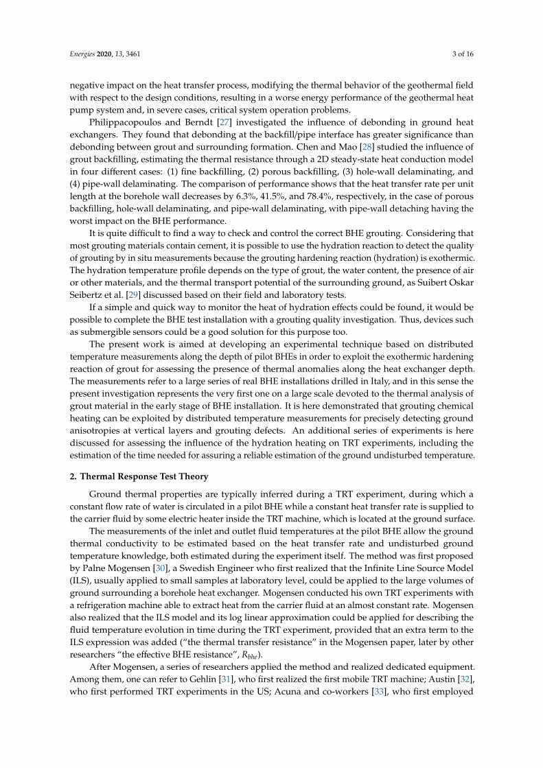
Figure 3. Schematics of the test system, including the heating cable and the submersible sensor movingalong one leg of the U-pipe.

The third component of the instrumentation is represented by manufacturer software able toprocess the data and configure the sensor.

The conversion of pressure into depth preventively requires information about the BHE length andthe offset water level within the pipe, together with the density of the fluid (in the present investigationtap water, 998 kg/m3). The sampling frequency has been set to 1 Hz in order to obtain one measurementevery 0.1 m approximately.

The submersible sensor has a known density of 1700 kg/m3, and the external software is able toestimate the sensor falling time based on the fluid and pipe data.

The dataset collected by the logger is sent to its validation box and then to the software thatconverts the measurements.

When the temperature measurements are employed for TRT analysis, the Equations (1)–(7) areapplied based on the knowledge of the applied heat flux provided by the heating cable. The calculationtool developed by the Authors is able to process measurements pertaining to given depths, thusinferring the ground conductivity kgr and the borehole effective resistance Rbhe layer by layer along theBHE depth for proper Forb windows.

Test Sites

The case studies presented in this paper refer to a series of real BHE fields located in northernItaly. All the measurements have been performed by the Geo-Net company. In the following, a seriesof identification codes will be employed.

Codes ASC-1 and ASC-2 refer to experiments carried out in Imola city (Italy, 44◦20′29.057′′ N;11◦43′23.46′′ E). Codes TAS-1 and TAS-2 refer to another pilot BHE in the same city (44◦20′50.64′′ N;11◦42′16.90′′ E). FAE-1 and FAE-2 are BHEs located in Faenza city (44◦17′27.06′′ N; 11◦52′3.85′′ E),and finally the PIS code refers to the city of Pistoia (43◦57′5.59′′ N; 10◦53′18.88′′ E).

A geological bibliography [44], confirmed by the geological surveys, showed that the ASC-1/2,TAS-1/2, and FAE-1/2 areas belong to the same geological context, which is characterized by continentalsedimentary deposits namely made by layers of gravel, sand, and silt. Concerning the PIS site, whichis in Tuscany, the geological surveys have shown shale rocks (argillite) surrounded by sedimentarysoils consisting of alluvial deposits.

Energies 2020, 13, 3461 8 of 16

The measurements refer to pilot BHEs constituted by double 32 mm U pipes, and they wereperformed between 2018 and 2020. All the boreholes are grouted ones, and the BHE nominal diameter is152 mm. The BHE depth is 120 m both in the ASC and PIS tests, whereas the TAS and FAE experimentswere performed with 110 m heat exchangers.

Regarding ASC-2, TAS-1/2, FAE-1/2, and PIS, the measurements refer to the assessment of thevertical ground temperature profiles at different times from grouting the borehole, and they representa series of snapshots of how the hydration heat can affect the ground undisturbed temperature profileand how such profiles can be employed for an indirect estimation of grouting defects.

Concerning the ASC-1 experiment, a distributed TRT has been performed on one pilot heatexchanger. Such a TRT refers to a series of temperature measurements along the BHE pipe when theelectric heater is releasing heat (at a constant rate) inside another pipe of the same BHE.

The adopted procedure was the following one. The TRT had a duration of more than 50 h,according to the recommendations available in [7]. Before activating the heating cable, a temperaturemeasurement is made with the travelling sensor to assess the undisturbed ground temperature as afunction of the depth, z (time zero). At this point, the electric cable is powered and a constant in thetime heat transfer rate is applied to the BHE. From that instant on, four more records (in the following,referred to as “logs”) are carried out after 3, 10, 23, and 50 h from the start of the heating part of the test.The heat transfer rate applied to the heating cable is 2400 W.

5. Results and Discussion

Preliminary measurements with the present experimental technique showed that after some 2 hfrom the beginning of the BHE grouting, a temperature perturbation can be detected along the BHEdepth. This behavior lasts up to 2 or 3 days after the BHE by grout. Figures 4 and 5 show the measuredtemperature profiles during the grout chemical reaction and after the end of it, some 10 days later.It can be noticed from both figures at the FAE site that the temperature increase (with respect to theundisturbed situation later in time) is almost uniform along the BHE depth, suggesting that the heatrelease rate per unit depth is uniform. It is worth noticing that, provided that the volumetric heatrelease is uniform as well, this temperature uniformity can suggest that the grouting was uniform involume all along the vertical direction.


position from the slope and intercept of the temperature profile when represented as a function of the logarithm of time. Table 1 shows some 8 of 1200 rows of data recorded during the experiment described in Figure 11. Columns 2 to 6 report the temperatures at several sampling times.

Figure 4. Vertical ground temperature profiles at the FAE-1 pilot borehole heat exchangers (BHE) during the grout hydration period (24 January profile) as compared to one at the end of the chemical reaction, 15 days later.

Figure 5. Vertical ground temperature profiles at the FAE-2 pilot BHE during the grout hydration period (24 January profile) as compared to the one at the end of the chemical reaction, 15 days later.

0

15

30

45

60

75

90

105

120

11 13 15 17 19 21

Dep

th [m

]

Fluid Temperature T [°C]

Log 24thJanuary 2019

Log 7thFebruary 2019

Grouting, 21thJanuary 2019

Undisturbed temperature profile

Temperature profile affected by grout chemical reaction

0

15

30

45

60

75

90

105

120

11 13 15 17 19 21

Dep

th [m

]


Log 24th January2019Log 7th Februrary2019Grouting, 23thJanuary 2019



0

15

30

45

60

75

90

105

120

11 13 15 17 19 21

Dep

th [m

]


Log 18thSeptember 2018Log 26thSeptember 2018Grouting, 18thSeptember

Cold zone

Figure 4. Vertical ground temperature profiles at the FAE-1 pilot borehole heat exchangers (BHE)during the grout hydration period (24 January profile) as compared to one at the end of the chemicalreaction, 15 days later.

Energies 2020, 13, 3461 9 of 16





0

15

30

45

60

75

90

105

120

11 13 15 17 19 21

Dep

th [m

]







0

15

30

45

60

75

90

105

120

11 13 15 17 19 21

Dep

th [m

]





0

15

30

45

60

75

90

105

120

11 13 15 17 19 21

Dep

th [m

]



Cold zone

Figure 5. Vertical ground temperature profiles at the FAE-2 pilot BHE during the grout hydrationperiod (24 January profile) as compared to the one at the end of the chemical reaction, 15 days later.

A different situation can be observed from inspecting Figures 6 and 7. Here, the measurementspertain to the PIS and TAS sites, respectively. In particular, Figure 6 shows a zone in the bottom BHEpart where the temperature does not change during the grout hydration period. The same can beobserved in Figure 7 at the BHE upper section. In both figures, this behavior has been named the “coldzone”, which in the experiment described in Figure 6 is related to depths from 55 m on. The presenceof cold zones can be observed in Figures 8 and 9 as well in the TAS and ASC measurements.

The presence of cold parts along the BHE depth has to be related to a lower local heat rate orto the absence of it. Furthermore, these low temperatures cannot be ascribed to local heat removalphenomena (e.g., advection), since all the measurements are made inside the grouted volume, whichthe pipes carrying the electric cable and the travelling sensor are embedded in. As a consequence, theonly possible explanation (or better, the more plausible one) is that any cold zone corresponds to apoor grouting, with the presence of air or water pockets.





0

15

30

45

60

75

90

105

120

11 13 15 17 19 21

Dep

th [m

]







0

15

30

45

60

75

90

105

120

11 13 15 17 19 21

Dep

th [m

]





0

15

30

45

60

75

90

105

120

11 13 15 17 19 21

Dep

th [m

]



Cold zone

Figure 6. Vertical ground temperature profiles at the PIS pilot BHE during the grout hydration period(18 September profile) as compared to the one at the end of the chemical reaction. A “cold zone”appears at both periods.

Energies 2020, 13, 3461 10 of 16


Figure 6. Vertical ground temperature profiles at the PIS pilot BHE during the grout hydration period (18 September profile) as compared to the one at the end of the chemical reaction. A “cold zone” appears at both periods.

Figure 7. Vertical ground temperature profiles at the TAS-1 pilot BHE during the grout hydration period (5 February profile) as compared to the one at the end of the chemical reaction. A “cold zone” appears at the top BHE.

Figure 8. Vertical ground temperature profiles at the ASC-2 BHE during the grout hydration period. A “cold zone” appears in the last 40 m.

0

15

30

45

60

75

90

105

120

11 13 15 17 19 21

Dep

th [m

]




Grouting, 4thFebruary 2020

Cold zone

0

15

30

45

60

75

90

105

120

11 13 15 17 19 21

Dep

th [m

]


Col

d zo

ne Log 5th March 2020 Grouting 3rd March 2020

Figure 7. Vertical ground temperature profiles at the TAS-1 pilot BHE during the grout hydrationperiod (5 February profile) as compared to the one at the end of the chemical reaction. A “cold zone”appears at the top BHE.


Figure 6. Vertical ground temperature profiles at the PIS pilot BHE during the grout hydration period (18 September profile) as compared to the one at the end of the chemical reaction. A “cold zone” appears at both periods.

Figure 7. Vertical ground temperature profiles at the TAS-1 pilot BHE during the grout hydration period (5 February profile) as compared to the one at the end of the chemical reaction. A “cold zone” appears at the top BHE.

Figure 8. Vertical ground temperature profiles at the ASC-2 BHE during the grout hydration period. A “cold zone” appears in the last 40 m.

0

15

30

45

60

75

90

105

120

11 13 15 17 19 21

Dep

th [m

]




Grouting, 4thFebruary 2020

Cold zone

0

15

30

45

60

75

90

105

120

11 13 15 17 19 21

Dep

th [m

]


Col

d zo

ne Log 5th March 2020 Grouting 3rd March 2020

Figure 8. Vertical ground temperature profiles at the ASC-2 BHE during the grout hydration period.A “cold zone” appears in the last 40 m.Energies 2020, 13, x FOR PEER REVIEW 11 of 16

Figure 9. Vertical ground temperature profiles at the TAS-2 BHE during the grout hydration period. A “cold zone” appears in between 13 and 35 m.

Columns A and B represent the slope m and intercept a of the ILS fitting line (Equation (6)), respectively. Furthermore, columns kgr and Rbhe provide estimates of the corresponding quantities at the given depth. Finally, the last row of Table 1 shows the averages of each column.

Figure 10. Vertical ground temperature profiles at the ASC-1 pilot BHE during the grout hydration period (19 September profile) as compared to the one at the end of the chemical reaction.

0

15

30

45

60

75

90

105

120

11 13 15 17 19 21

Dep

th [m

]


Cold zone

Log 17th February 2020 Grouting 14th February 2020

0

15

30

45

60

75

90

105

120

11 13 15 17 19 21

Dep

th [m

]


Log 19th March2020

Log 20th March2020

Log 31th March2020

Grouting, 19thMarch 2020

Figure 9. Vertical ground temperature profiles at the TAS-2 BHE during the grout hydration period.A “cold zone” appears in between 13 and 35 m.

Energies 2020, 13, 3461 11 of 16

In order to perform a reliable distributed TRT, it is necessary to record the temperature valueswhen the hydration reaction is completed and the extra heat effects have vanished. To establish whenthe TRT experiment can be started, several temperature logs with the submersible sensor have beenperformed. This procedure is the one described in Figure 10 for the ASC site.


Figure 9. Vertical ground temperature profiles at the TAS-2 BHE during the grout hydration period. A “cold zone” appears in between 13 and 35 m.

Columns A and B represent the slope m and intercept a of the ILS fitting line (Equation (6)), respectively. Furthermore, columns kgr and Rbhe provide estimates of the corresponding quantities at the given depth. Finally, the last row of Table 1 shows the averages of each column.

Figure 10. Vertical ground temperature profiles at the ASC-1 pilot BHE during the grout hydration period (19 September profile) as compared to the one at the end of the chemical reaction.

0

15

30

45

60

75

90

105

120

11 13 15 17 19 21

Dep

th [m

]


Cold zone

Log 17th February 2020 Grouting 14th February 2020

0

15

30

45

60

75

90

105

120

11 13 15 17 19 21D

epth

[m]


Log 19th March2020

Log 20th March2020

Log 31th March2020

Grouting, 19thMarch 2020

Figure 10. Vertical ground temperature profiles at the ASC-1 pilot BHE during the grout hydrationperiod (19 September profile) as compared to the one at the end of the chemical reaction.

Figure 10 shows that the hydration heat is active in the first days from grouting and that theundisturbed condition is reached in some 12 days (red curve).

Figure 11 shows the measurements in the ASC-1 experiment after the complete decay ofany hydration effect. In this case, the distributed TRT experiment lasted 50 h, during which thetravelling sensor was inserted 4 times inside the pipe for recording the temperature and pressure.The measurements have been recorded approximately every 0.1 m, and the complete record hencecontains thousands of data points. By performing the analysis described by Equations (5)–(7), itwas possible to infer the ground thermal conductivity and borehole thermal resistance at each depthposition from the slope and intercept of the temperature profile when represented as a function ofthe logarithm of time. Table 1 shows some 8 of 1200 rows of data recorded during the experimentdescribed in Figure 11. Columns 2 to 6 report the temperatures at several sampling times.Energies 2020, 13, x FOR PEER REVIEW 12 of 16

Figure 11. Distributed Thermal Response Test (TRT) experiment at the ASC site after the complete decay of any hydration effect. Vertical temperature profiles along the BHE depth during a 50 h experiment at a constant heat transfer rate.

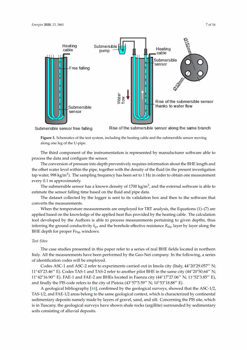
Table 1. A selection of the dataset containing all the measured temperatures in time and space. Column A and B are the Infinite Line Source (ILS) model estimations for the slope and intercept, respectively (Equation 5), as obtained by log-linear regression for each row. Columns kgr and Rbhe are the estimates for the ground and BHE properties as solutions of Equation (7) applied to each row.

Depth T at 0 h T at 3 h T at 8 h T at 23 h T at 50 h A B kgr Rbhe 1.4 14.54 14.85 15.94 16.21 16.91 0.682 8.676 2.335 0.150 1.5 14.54 14.85 15.94 16.21 16.91 0.722 8.194 2.206 0.169 1.6 14.54 14.85 15.94 16.21 16.91 0.725 8.098 2.196 0.175 1.7 14.54 14.85 15.94 16.21 16.91 0.726 8.049 2.193 0.178 [---] [---] [---] [---] [---] [---] [---] [---] [---] [---] 118.7 14.47 15.45 16.17 16.81 17.06 0.587 10.089 2.713 0.096 118.8 14.47 15.41 16.12 16.75 16.96 0.567 10.234 2.806 0.093 118.9 14.48 15.33 16.06 16.59 16.85 0.547 10.345 2.909 0.092 119.0 14.47 15.28 15.93 16.51 16.56 0.480 10.926 3.316 0.076

Average 16.01 16.91 17.70 18.23 16.08 0.772 8.965 2.064 0.119

Figure 12 shows the results of such an analysis. In particular, Figure 12 shows that at a given depth layer (about 65 m), the estimated parameters are significantly different from those at other locations, thus allowing one to guess that that ground layer is characterized by groundwater circulation, which is able to enhance the local heat transfer in terms of a higher (apparent) ground conductivity.

0

15

30

45

60

75

90

105

120

11 13 15 17 19 21

Dep

th [m

]


Log 31th March2020 [0 hours]



Log 1st April2020 [23 hours]

Log 2nd April2020 [50 hours]

Figure 11. Distributed Thermal Response Test (TRT) experiment at the ASC site after the complete decayof any hydration effect. Vertical temperature profiles along the BHE depth during a 50 h experiment ata constant heat transfer rate.

Energies 2020, 13, 3461 12 of 16

Table 1. A selection of the dataset containing all the measured temperatures in time and space. ColumnA and B are the Infinite Line Source (ILS) model estimations for the slope and intercept, respectively(Equation 5), as obtained by log-linear regression for each row. Columns kgr and Rbhe are the estimatesfor the ground and BHE properties as solutions of Equation (7) applied to each row.

Depth T at 0 h T at 3 h T at 8 h T at 23 h T at 50 h A B kgr Rbhe

1.4 14.54 14.85 15.94 16.21 16.91 0.682 8.676 2.335 0.1501.5 14.54 14.85 15.94 16.21 16.91 0.722 8.194 2.206 0.1691.6 14.54 14.85 15.94 16.21 16.91 0.725 8.098 2.196 0.1751.7 14.54 14.85 15.94 16.21 16.91 0.726 8.049 2.193 0.178[—] [—] [—] [—] [—] [—] [—] [—] [—] [—]

118.7 14.47 15.45 16.17 16.81 17.06 0.587 10.089 2.713 0.096118.8 14.47 15.41 16.12 16.75 16.96 0.567 10.234 2.806 0.093118.9 14.48 15.33 16.06 16.59 16.85 0.547 10.345 2.909 0.092119.0 14.47 15.28 15.93 16.51 16.56 0.480 10.926 3.316 0.076

Average 16.01 16.91 17.70 18.23 16.08 0.772 8.965 2.064 0.119

Columns A and B represent the slope m and intercept a of the ILS fitting line (Equation (6)),respectively. Furthermore, columns kgr and Rbhe provide estimates of the corresponding quantities atthe given depth. Finally, the last row of Table 1 shows the averages of each column.

Figure 12 shows the results of such an analysis. In particular, Figure 12 shows that at a given depthlayer (about 65 m), the estimated parameters are significantly different from those at other locations,thus allowing one to guess that that ground layer is characterized by groundwater circulation, whichis able to enhance the local heat transfer in terms of a higher (apparent) ground conductivity.Energies 2020, 13, x FOR PEER REVIEW 13 of 16

(a) (b)

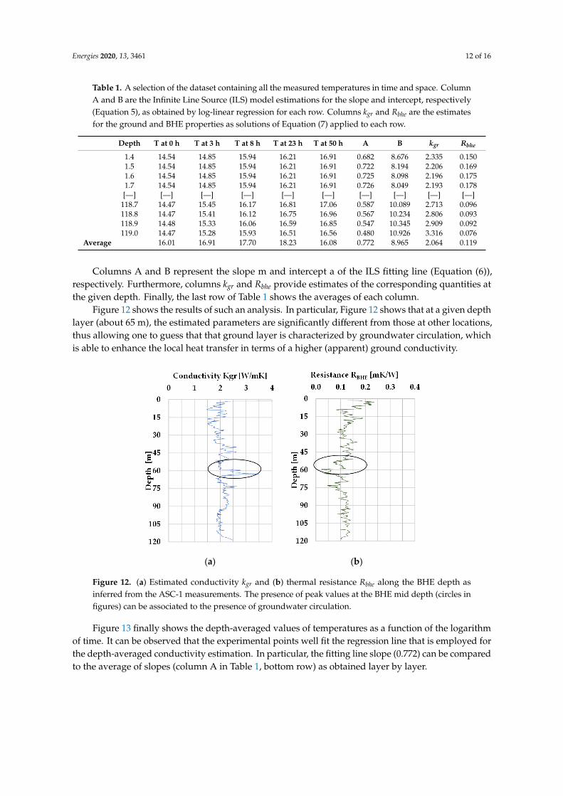
Figure 12. (a) Estimated conductivity kgr and (b) thermal resistance Rbhe along the BHE depth as inferred from the ASC-1 measurements. The presence of peak values at the BHE mid depth (circles in figures) can be associated to the presence of groundwater circulation.

Figure 13 finally shows the depth-averaged values of temperatures as a function of the logarithm of time. It can be observed that the experimental points well fit the regression line that is employed for the depth-averaged conductivity estimation. In particular, the fitting line slope (0.772) can be compared to the average of slopes (column A in Table 1, bottom row) as obtained layer by layer.

The same analysis can be made in terms of the fitting line intercept (8.965 in Figure 13) and the corresponding average value in Table 1 (column B, bottom row). It is apparent from such a comparison that average kgr and Rbhe values as estimated with both methods are very similar, and their agreement is within 1%, thus providing a cross validation of the whole experimental procedure.

Figure 13. Depth-averaged temperatures as the function of the logarithm of time. The fitting line is employed for a depth-averaged conductivity estimation.

y = 0.7718x + 8.9646R² = 0.9999

15.5

16.0

16.5

17.0

17.5

18.0

18.5

19.0

8 9 10 11 12 13

Flui

d Te

mpe

ratu

re [°

C]

Logarithm of Time [-]

Figure 12. (a) Estimated conductivity kgr and (b) thermal resistance Rbhe along the BHE depth asinferred from the ASC-1 measurements. The presence of peak values at the BHE mid depth (circles infigures) can be associated to the presence of groundwater circulation.

Figure 13 finally shows the depth-averaged values of temperatures as a function of the logarithmof time. It can be observed that the experimental points well fit the regression line that is employed forthe depth-averaged conductivity estimation. In particular, the fitting line slope (0.772) can be comparedto the average of slopes (column A in Table 1, bottom row) as obtained layer by layer.

Energies 2020, 13, 3461 13 of 16


(a) (b)

Figure 12. (a) Estimated conductivity kgr and (b) thermal resistance Rbhe along the BHE depth as inferred from the ASC-1 measurements. The presence of peak values at the BHE mid depth (circles in figures) can be associated to the presence of groundwater circulation.

Figure 13 finally shows the depth-averaged values of temperatures as a function of the logarithm of time. It can be observed that the experimental points well fit the regression line that is employed for the depth-averaged conductivity estimation. In particular, the fitting line slope (0.772) can be compared to the average of slopes (column A in Table 1, bottom row) as obtained layer by layer.

The same analysis can be made in terms of the fitting line intercept (8.965 in Figure 13) and the corresponding average value in Table 1 (column B, bottom row). It is apparent from such a comparison that average kgr and Rbhe values as estimated with both methods are very similar, and their agreement is within 1%, thus providing a cross validation of the whole experimental procedure.

Figure 13. Depth-averaged temperatures as the function of the logarithm of time. The fitting line is employed for a depth-averaged conductivity estimation.

y = 0.7718x + 8.9646R² = 0.9999

15.5

16.0

16.5

17.0

17.5

18.0

18.5

19.0

8 9 10 11 12 13

Flui

d Te

mpe

ratu

re [°

C]

Logarithm of Time [-]

Figure 13. Depth-averaged temperatures as the function of the logarithm of time. The fitting line isemployed for a depth-averaged conductivity estimation.

The same analysis can be made in terms of the fitting line intercept (8.965 in Figure 13) and thecorresponding average value in Table 1 (column B, bottom row). It is apparent from such a comparisonthat average kgr and Rbhe values as estimated with both methods are very similar, and their agreementis within 1%, thus providing a cross validation of the whole experimental procedure.

6. Conclusions

A series of experiments have been performed in a pilot BHE located in northern Italy during theperiod 2018–2020. Such measurements have been realized by means of submergible sensors able torecord the local temperature along the BHE depth with a spatial step of less than 0.5 m and typicallyequal to 0.1 m. The temperature profiles along the vertical directions have been employed for a doubleanalysis. The first part of the present investigation was devoted to assessing the effects of the hydrationheat released by the grouting cement. It is here demonstrated that the grout chemical reaction canincrease the local ground temperature close to the BHE pipes by up to 1.5 ◦C, and that this effectvanishes after a period ranging from 10 days to 2 weeks.

The same measurements have been employed for detecting the presence of “cold zones” along theborehole heat exchanger, where the local temperature does not change in time during the hydrationperiod, when chemical heat release is expected.

The presence of cold zones is here ascribed to the lack of chemical reactions due to poor groutingor, in other words, to the presence of air, water, or gravel pockets in certain stretches of the BHE volume.In this sense, the present distributed measurement technique offers interesting opportunities forchecking the quality of the grouting process in order to assess and forecast the BHE future performance.

The distributed temperature measurements have been finally employed for electrical heating TRTexperiments. In this case, pipes are filled by water and one of them if fitted with the electric cable,while the other is used to sink the travelling sensor. It is here confirmed that the technique can beapplied with the standard set of equations described by the ILS theory in order to estimate the local(depth related) values of both the ground thermal conductivity and the BHE thermal resistance.

Author Contributions: G.C. and C.P.: measurements; F.M.: hydration parts and results presentation; M.F.:theoretical analysis and general manuscript organization. All authors have read and agreed to the publishedversion of the manuscript.

Funding: This research received no external funding.

Acknowledgments: A.P. and S.M., at Dime, are acknowledged for their contribution in reviewing the presentpaper and their useful suggestions for improving it.

Conflicts of Interest: The authors declare no conflict of interest.

Energies 2020, 13, 3461 14 of 16

Nomenclature

Symbol Variable UnitBHE Borehole Heat Exchanger -TRT Thermal Response Test -kgr the effective ground thermal conductivity W/(m K)Rbhe effective borehole thermal resistance (m K)/WQ’ heat transfer rate per unit length W/mr radial distance from the line source Mrb borehole radius MFo Fourier number -τ time ST Temperature ◦CTf,ave average fluid temperature ◦CTgr,∞ undisturbed ground temperature ◦C

References

1. Aranzabal, N.; Martos, J.; Steger, H.; Blum, P.; Soret, J. Temperature measurements along a vertical boreholeheat exchanger: A method comparison. Renew. Energy 2019, 143, 1247–1258. [CrossRef]

2. Zeng, H.; Diao, N.; Fang, Z. Efficiency of vertical geothermal heat exchangers in the ground source heatpump system. J. Therm. Sci. 2003, 12, 77–81. [CrossRef]

3. Luo, J.; Rohn, J.; Bayer, M.; Priess, A. Thermal performance and economic evaluation of double U-tubeborehole heat exchanger with three different borehole diameters. Energy Build. 2013, 67, 217–224. [CrossRef]

4. Sutton, M.G.; Nutter, D.W.; Couvillion, R.J. A ground resistance for vertical bore heat exchangers withgroundwater flow. J. Energy Resour. Technol. 2003, 125, 183–189. [CrossRef]

5. Wagner, V.; Blum, P.; Kübert, M.; Bayer, P. Analytical approach to groundwater influenced thermal responsetests of grouted borehole heat exchangers. Geothermics 2013, 46, 22–31. [CrossRef]

6. IEA ECES, Annex 21. Thermal Response Test. Available online: http://projects.gtk.fi/Annex21/homepage.htm(accessed on 18 May 2020).

7. UNI—Ente Nazionale di Unificazione, UNI 11466:2012. Sistemi Geotermici a Pompa di Calore—Requisiti per ilDimensionamento e la Progettazione; Ente Nazionale di Unificazione: Milan, Italy, 2012.

8. Stauffer, F.; Bayer, P.; Blum, P.; Molina-Giraldo, N.; Kinzelbach, W. Thermal Use of Shallow Groundwater; CRCPress: Boca Raton, FL, USA, 2013. [CrossRef]

9. Bandos, T.V.; Montero, Á.; Fernández, E.; Santander, J.L.G.; Isidro, J.M.; Pérez, J.; de Córdoba, P.J.F.;Urchueguía, J.F. Finite line-source model for borehole heat exchangers: Effect of vertical temperaturevariations. Geothermics 2009, 38, 263–270. [CrossRef]

10. Martos, J.; Montero, A.; Torres, J.; Soret, J.; Martínez, G.; García-Olcina, R. Novel wireless sensor system fordynamic characterization of borehole heat exchangers. Sensors 2011, 11, 7082–7094. [CrossRef]

11. GEOsniff®Geothermal Monitoring Innovative and Miniaturized. Available online: https://www.enoware.de/en/products/geosniff/ (accessed on 16 May 2020).

12. Aranzabal, N.; Martos, J.; Stokuca, M.; Mazzotti Pallard, W.; Acuña, J.; Soret, J.; Blum, P. Novel instrumentsand methods to estimate depth-specific thermal properties in borehole heat exchangers. Geothermics 2020, 86,101813. [CrossRef]

13. Hellström, G. Ground Heat Storage. Thermal Analysis of Duct Storage Systems: Theory. Ph.D. Thesis,University of Lund, Lund, Sweden, 1991.

14. Paul, N.D. The Effect of Grout Thermal Conductivity on Vertical Geothermal Heat Exchanger Design andPerformance. Master’s Thesis, South Dakota State University, Brookings, South Dakota, 1996.

15. Zeng, H.; Diao, N.; Fang, Z. Heat transfer analysis of boreholes in vertical ground heat exchangers. Int. J.Heat Mass Transf. 2003, 46, 4467–4481. [CrossRef]

16. IGHSPA. Grouting for Vertical Geothermal Heat Pump Systems: Engineering Design and Field Procedures Manual;Electric Power Research Institute (EPRI)—IGHSPA: Stillwater, Oklahoma, 2000.

17. UNI—Ente Nazionale di Unificazione, UNI 11467:2012. Sistemi Geotermici a Pompa di Calore—Requisiti perL’installazione; Ente Nazionale di Unificazione: Milan, Italy, 2012.

http://dx.doi.org/10.1016/j.renene.2019.05.092

http://dx.doi.org/10.1007/s11630-003-0012-1

http://dx.doi.org/10.1016/j.enbuild.2013.08.030

http://dx.doi.org/10.1115/1.1591203

http://dx.doi.org/10.1016/j.geothermics.2012.10.005

http://projects.gtk.fi/Annex21/homepage.htm

http://dx.doi.org/10.1201/b16239


http://dx.doi.org/10.3390/s110707082

https://www.enoware.de/en/products/geosniff/

https://www.enoware.de/en/products/geosniff/

http://dx.doi.org/10.1016/j.geothermics.2020.101813

http://dx.doi.org/10.1016/S0017-9310(03)00270-9

Energies 2020, 13, 3461 15 of 16

18. Verein Deutscher Ingenieure-VDI, VDI 4640 Blatt 2:2019. Thermal Use of Underground—Ground Source HeatPump Systems; Verein Deutscher Ingenieure: Düsseldorf, Germany, 2019.

19. Claesson, J.; Hellström, G. Multipole method to calculate borehole thermal resistances in a borehole heatexchanger. HVAC R Res. 2011, 17, 895–911. [CrossRef]

20. Lamarche, L.; Kajl, S.; Beauchamp, B. A review of methods to evaluate borehole thermal resistances ingeothermal heat-pump systems. Geothermics 2010, 39, 187–200. [CrossRef]

21. Rees, S. Advances in Ground-Source Heat Pump Systems, 1st ed.; Woodhead Publishing: Sawston, UK, 2016;ISBN 9780081003114.

22. Berndt, M.; Kavanaugh, S. Thermal Conductivity of Cementitious Grouts and Impact on Heat ExchangerLength Design for Ground Source Heat Pumps. HVAC R Res. 1999, 5, 85–96. [CrossRef]

23. Hossein, J.; Seyed, M.A.; Rosen, M.; Pourfallah, M. A comprehensive review of backfill materials and theireffects on ground heat exchanger performance. Sustainability 2018, 10, 4486. [CrossRef]

24. Delaleux, F.; Py, X.; Olives, R.; Dominguez, A. Enhancement of geothermal borehole heat exchangersperformances by improvement of bentonite grouts conductivity. Appl. Therm. Eng. 2012, 33, 92–99.[CrossRef]

25. Alrtimi, A.A.; Rouainia, M.; Manning, D.A.C. Thermal enhancement of PFA-based grout for geothermal heatexchangers. Appl. Therm. Eng. 2013, 54, 559–564. [CrossRef]

26. Chen, F.; Mao, J.; Chen, S.; Li, C.; Hou, P.; Liao, L. Efficiency analysis of utilizing phase change materials asgrout for a vertical U-tube heat exchanger coupled ground source heat pump system. Appl. Thermal Eng.2018, 130, 698–709. [CrossRef]

27. Philippacopoulos, A.J.; Berndt, M.L. Influence of debonding in ground heat exchangers used with geothermalheat pumps. Geothermics 2001, 30, 527–545. [CrossRef]

28. Chen, S.; Mao, J. Quantitative evaluation of improper backfilling in vertical borehole. J. Therm. Sci. Technol.2016, 11, JTST00018. [CrossRef]

29. Suibert Oskar Seibertz, K.; Händel, F.; Dietrich, P.; Vienken, T. On the use of hydration heat for qualitymanagement of borehole heat exchanger grouting. In Proceedings of the EGU General Assembly ConferenceAbstracts, EGU General Assembly, Vienna, Austria, 17–22 April 2016; p. EPSC2016-12711. Available online:https://ui.adsabs.harvard.edu/abs/2016EGUGA.1812711S (accessed on 18 May 2020).

30. Mogensen, P. Fluid to duct wall heat transfer in duct system heat storages. Doc. Swed. Counc. Build. Res.1983, 16, 652–657.

31. Gehlin, S. Thermal Response Test Method Development and Evaluation. Ph.D. Thesis, Lulea University ofTechnology, Lulea, Sweden, 1996.

32. Austin, W.A. Development of an In Situ System for Measuring ground Thermal Properties. Ph.D. Thesis,Oklahoma State University, Stillwater, Oklahoma, 1998.

33. Acuna, J.; Mogensen, P.; Palm, B. Distributed thermal response test on a U-pipe borehole heat exchanger.In Proceedings of the 11th International Conference on Energy Storage, EFFSTOCK, Stockholm, Sweden,16 June 2009.

34. Fossa, M.; Rolando, D.; Pasquier, P. Pulsated Thermal Response Test experiments and modelling for groundthermal property estimation. In Proceedings of the International Ground Source Heat Pump AssociationResearch Conference, Stockholm, Sweden, 18–20 September 2018; pp. 220–228. [CrossRef]

35. Morchio, S.; Fossa, M. On the ground thermal conductivity estimation with coaxial borehole heat exchangersaccording to different undisturbed ground temperature profiles. Appl. Therm. Eng. 2020. [CrossRef]

36. Fossa, M.; Priarone, A.; Silenzi, F. Superposition of the Single Point Source Solution to Generate TemperatureResponse Factors for Geothermal Piles. Renew. Energy 2020, 145, 805–813. [CrossRef]

37. Franco, A.; Conti, P. Clearing a Path for Ground Heat Exchange Systems: A Review on Thermal ResponseTest (TRT) Methods and a Geotechnical Routine Test for Estimating Soil Thermal Properties. Energies 2020,13, 2965. [CrossRef]

38. Ingersoll, L.R.; Zobel, O.J.; Ingersoll, A.C. Heat Conduction with Engineering, Geological, and Other Applications;McGraw-Hill: New York, NY, USA, 1954.

39. Fossa, M. Correct Design of Vertical BHE Systems through the Improvement of the Ashrae Method. Sci. Technol.Built Environ. 2016, 23, 1080–1089. [CrossRef]

40. Eskilson, P. Thermal Analysis of Heat Extraction Boreholes. Ph.D. Thesis, Lund University of Technology,Lund, Sweden, 1987.

http://dx.doi.org/10.1080/10789669.2011.609927


http://dx.doi.org/10.1080/10789669.1999.10391226

http://dx.doi.org/10.3390/su10124486

http://dx.doi.org/10.1016/j.applthermaleng.2011.09.017



http://dx.doi.org/10.1016/S0375-6505(01)00011-6

http://dx.doi.org/10.1299/jtst.2016jtst00018

https://ui.adsabs.harvard.edu/abs/2016EGUGA.1812711S

http://dx.doi.org/10.22488/okstate.18.000021

http://dx.doi.org/10.1016/j.applthermaleng.2020.115198

http://dx.doi.org/10.1016/j.renene.2019.05.011

http://dx.doi.org/10.3390/en13112965

http://dx.doi.org/10.1080/23744731.2016.1208537

Energies 2020, 13, 3461 16 of 16

41. Hu, J.; Ge, Z.; Wang, K. Influence of cement fineness and water-to-cement ratio on mortar early-age heat ofhydration and set times. Constr. Build. Mater. 2014, 50, 657–663. [CrossRef]

42. Kavanaugh, S.P. Field Tests for Ground Thermal Properties—Methods and Impact on Ground-Source HeatPump Design. ASHRAE Trans. 2000, 106, 851–855.

43. ASHRAE. ASHRAE Fundamentals Handbook; ASHRAE: Atlanta, GA, USA, 2007; Chapter A32.44. Geoportale Regione Emilia-Romagna. Available online: https://geoportale.regione.emilia-romagna.it/

(accessed on 22 May 2020).

© 2020 by the authors. Licensee MDPI, Basel, Switzerland. This article is an open accessarticle distributed under the terms and conditions of the Creative Commons Attribution(CC BY) license (http://creativecommons.org/licenses/by/4.0/).

http://dx.doi.org/10.1016/j.conbuildmat.2013.10.011

https://geoportale.regione.emilia-romagna.it/

http://creativecommons.org/

http://creativecommons.org/licenses/by/4.0/.

experimental hydration temperature increase in borehole

Documents