Technical Report

TR-06-07

ISSN 1404-0344CM Digitaltryck AB, Bromma, 2006

Experimental determination and chemical modelling of radiolytic processes at the spent fuel/water interface

Long contact time experiments

Esther Cera, Jordi Bruno, Lara Duro

ENVIROS SPAIN, SL, Barcelona, Spain

Trygve Eriksen

Dept Nuclear Chemistry, KTH, Stockholm, Sweden

Svensk Kärnbränslehantering ABSwedish Nuclear Fueland Waste Management CoBox 5864SE-102 40 Stockholm Sweden Tel 08-459 84 00 +46 8 459 84 00Fax 08-661 57 19 +46 8 661 57 19

Experimental determination and chemical modelling of radiolytic processes at the spent fuel/water interface

Long contact time experiments

Esther Cera, Jordi Bruno, Lara Duro

ENVIROS SPAIN, SL, Barcelona, Spain

Trygve Eriksen

Dept Nuclear Chemistry, KTH, Stockholm, Sweden

Keywords: Radionuclides, Radiolysis products, Spent fuel, Thermodynamic.

This report concerns a study which was conducted for SKB. The conclusions and viewpoints presented in the report are those of the authors and do not necessarily coincide with those of the client.

A pdf version of this document can be downloaded from www.skb.se

�

Abstract

We report on the last experimental and modelling results of a research programme that started in 1995, corresponding in that case to the long contact time experiments. The aim of this programme has been to understand the processes that control the radiolytic genera-tion of oxidants and reductants at the spent fuel water interface and their consequences for spent fuel stability and radionuclide release. The results of this work have been reported in different papers and technical reports during the last decade, /Eriksen et al. 1995, Bruno et al. 1999, 200�/. In this series, well controlled dissolution experiments of PWR Ringhals spent fuel fragments in an initially anoxic closed system and by using different solution compositions have been carried out, the experiments have been opened after a long time period (between 1.5 and � years), samples have been taken and gas and solution analyses have been performed.

The results indicate the following:• Hydrogen and oxygen concentrations follow the same trend, an initial increase of the

concentration of both compounds with time until they reach a steady state that indicates an overall balance of all the radiolytic species generated in the system. Hydrogen peroxide data show in general an initial decrease with time until it reaches a steady state for a given solution composition. This confirms the overall balance of the generated radiolytic species.

• The experimental data shows that uranium dissolution is controlled by the oxidation of the UO2 matrix in 10 mM bicarbonate solutions while in the rest of the tests carried out at lower or in the absence of carbonate, uranium in the aqueous phase is governed by the precipitation of schoepite. These processes control the co-dissolution of most of the analysed radionuclides, including Sr, Cs, Mo, Tc and Np while not a clear dependency is found for Pu, Y, and Nd suggesting that other processes are governing the concentration of these radionuclides in the aqueous phase.

Kinetic modelling has been performed with data from experiments carried out at 10 mM of carbonate in the leaching solution. The data used have been uranium and the trace element concentrations which are congruently released. Radiolytic calculations on the studied systems are presented in the Appendix.

�

Sammanfattning

I rapporten redovisas de senaste experimentella och modellerings resultaten från en serie långtids försök (1.5–� år) inom ramen för ett forskningsprogram som startades 1995.

Målsättningen för programmet är ökad förståelse för radiolytisk bildning av oxidanter och reduktanter vid bränsleytan och deras inverkan på matrisupplösning och frigöring av radionuklider. Tidigare erhållna resultat har redovisats i flera rapporter och publikationer; /Eriksen et al. 1995, Bruno et al. 1999, 200�/.

Långtidsförsöken har genomförts med Ringhals bränslefragment och Ar-mättade karbonat haltiga lösningar i slutna ampuller. Vid försökens slut har ampullerna öppnats och analyser av gasfas och lösningar genomförts.

Experimentella data visar följande:• Väte och syre koncentrationernas tidsberoende är likartade, en initial ökning av koncen-

trationen följs av fortfarighetstillstånd med koncentrationer som indikerar massbalans av radiolytiskt bildade reaktanter i systemet. Väteperoxiden ställer snabbt in sig på en låg koncentration.

• Urankoncentrationen i 10 mM bikarbonatlösning styrs av UO2-matrisens oxidation och upplösning. Vid lägre bikarbonat koncentrationer fälls uran ut som schoepit. Medupplösningen av flertalet av de analyserade radionukliderna inklusive Sr, Cs, Mo, Tc och Np följer uranupplösningen. Pu, Y och Np koncentrationernas tidsberoende visar på att andra processer kontrollerar dessa nukliders koncentration i lösningen.

Beräkningar baserade på radiolys, homogen kinetik och oxidation av bränsleytan med väteperoxid och karbonatradikal (CO�

–×) presenteras i Appendix. De beräknade koncentra-tionerna av väte och syre i gasfasen samt väteperoxid och uran i lösningen är, inom ramen för osäkerheterna i experimentella data och modellantaganden, i god överensstämmelse med experimentellt mätta koncentrationer vid försökens slut. Enligt beräkningerna har emellertid fortfarighetstillstånd ej uppnåtts i systemet.

5

Contents

1 Introduction 7

2 Experimental 92.1 Material 92.2 Experimental set up 92.� Gas and solution analyses 10

3 Results 11�.1 Radiolysis products 11

�.1.1 Comparison with the previous series of experiments. Time resolved and long term experiments 1�

�.2 Radionuclide concentration in solution 15�.2.1 Actinides 15�.2.2 Fission products 16�.2.� Comparison with the previous series of experiments. Time

resolved and long term experiments 17

4 Datatreatmentanddiscussion 21�.1 Kinetic approaches for radiolysis products 21

�.1.1 Hydrogen 21�.1.2 Oxygen 2��.1.� Hydrogen peroxide 2�

�.2 Estimation of the redox conditions 25�.� Thermodynamic and kinetic approaches for radionuclides release 28

�.�.1 Tests carried out with a higher carbonate content in the leaching solution 28

�.�.2 Tests carried out with a low concentration or without carbonates in the leaching solution �0

5 Conclusions �7

6 References �9

Appendix1 Radiolytic modelling of time resolved and long contact time experiments 51

7

1 Introduction

The geochemical stability of a nuclear waste repository largely depends on the appropriate conditions for the stability and performance of the successive barriers of the repository system. The spent fuel matrix is the first barrier within the repository design given the high stability of this material in anoxic media. Consequently, one of the critical parameters to define the stability of the spent fuel matrix in a repository design is the redox potential, measured as Eh. The confinement of radionuclides within the matrix is guaranteed if the oxidation state of the UO2 matrix does not exceed the upper limit of stability of the cubic structure, UO2.��, which corresponds to a nominal stoichiometry of U�O7 /Johnson and Shoesmith 1988, Shoesmith 2000/, consequently its stability will depend on the ability of the oxidant species to oxidise the UO2 matrix to an oxidation state above this limit.

In this context, it is important to stress that the spent fuel matrix is a dynamic redox system by itself given the generation of oxidants and reductants at the fuel/water interface due to α, β and γ radiolysis. Therefore, it is problematic to treat the spent fuel/water system as redox equilibrium and it is more appropriate to study this system in terms of redox capacities.

The active role of the UO2 surfaces in poising the redox capacity in the spent fuel/water interface has been studied in the last years within the research programme started in 1995. The results of this experimental work have crystallised in several publications and technical reports, /Eriksen et al. 1995, Bruno et al. 200�/.

This work is the continuation of this experimental and modelling programme since new series of experiments, the so-called long contact time experiments, started at the end of the year 1999. The first ampoules were opened in mid year 2001, opening the last ones at the end of October 2002. Several solution compositions have been used in this series, bicar-bonate, bicarbonate plus chloride, chloride and Allard groundwater in order to ascertain the role of the composition of the leaching solution combined with water radiolysis on the alteration of the matrix and radionuclide release at long time periods.

The objective of this report is to present the new experimental data and modelling work referred to the last experimental series together with the ones reported in the previous work /Bruno et al. 200�/. In addition to the chemical modelling, a radiolytic modelling of the systems studied has been presented in the Appendix.

9

2 Experimental

2.1 MaterialFragments from a PWR fuel rod with a calculated burnup of �0 MWd/kgU were used. The weight of the fragments in each experiment was 1.0� ± 0.0� g. Fragment sizes ranged between 0.25 and � mm depending on the tests (see Table 2-1) and surface areas were calculated by means of the geometric surface areas multiplied with a roughness factor of �. Test solutions were prepared from Milli-Q purified water purged with AGA 5.7 quality argon, containing less than 0.5 ppm oxygen. NaHCO� and NaCl PA quality were used.

2.2 ExperimentalsetupThe ampoules used had a breakable glass membrane and a total volume of approximately 60 cm�. The ampoules, containing fuel fragments, were placed in a lead shield in a glove box with argon atmosphere and flushed with argon, Following this procedure �0 cm� solution was transferred to each ampoule and the ampoules sealed by localized heating using a specially designed electric oven. Different solution compositions were used in this series of experiments as specified in Table 2-1. The ampoules were stored for periods ranging between �97 and 917 days as shown in Table 2-1.

Table2-1. Initialsolutioncompositionandstoragetimeofeachrun.

Ampoule Solutioncomposition Storagetime(days)

1 10 mM NaHCO3 9103 10 mM NaHCO3 766

4 10 mM NaHCO3 4395 10 mM NaHCO3 7616 10 mM NaHCO3 4367 10 mM NaHCO3 + 2 mM NaCl 4328 10 mM NaHCO3 + 2 mM NaCl 7539 10 mM NaHCO3 + 2 mM NaCl 42710 10 mM NaHCO3 + 2 mM NaCl 92311 2 mM NaCl 39712 2 mM NaCl 71313 2 mM NaCl 41014 2 mM NaCl 88615 allard GW 43116 allard GW 74617 allard GW 42618 allard GW 91719 10 mM NaHCO3 432

10

After each storage period, ampoules were moved and connected to the gas analysing system. The ampoule membranes were broken and the gas phase analysed for oxygen and hydrogen as described below. Following the gas analysis, solution samples were analysed for hydrogen peroxide, uranium and minor components of the fuel.

Uranium was also analysed from strip solutions in some of the tests.

2.3 GasandsolutionanalysesThe glass ampoule was connected to a gas sampling system with a small pre-evacuated metal sampling cell and the ampoule membrane broken. Following pressure equalization in the system the sampling cell was closed and thereafter transferred to a mass spectrometer for analysis of radiolytically formed hydrogen and oxygen. The analytic procedure was calibrated using standard gas mixtures.

Hydrogen peroxide was measured by means of a luminescence method earlier described in detail by /Eriksen et al. 1995/. Fission products were analysed with ICP-MS (Plasma Quad 2 Plus, VG Elemental UK) as described earlier in /Bruno et al. 1999/. The uranium concentration was also measured using laser fluorimetry (Scintrex UA-�).

11

3 Results

3.1 RadiolysisproductsThe concentrations of oxygen, hydrogen peroxide and hydrogen measured at the end of the dissolution period in each ampoule are given in Figure �-1.

As we can see the concentration of hydrogen is, within the experimental uncertainties, quite constant in all the ampoules independently on the solution composition and dissolu-tion time. This indicates that the concentration of this reductant species reached steady state after some time of contact with the leach solution. This behaviour was not observed in the time resolved experiment with short contact times (< 20 days) where a continuous increase of the hydrogen concentration occurred for all the experimental period of those tests /Bruno et al. 200�/.

Oxygen concentrations obtained from the different ampoules follow the same trend as for hydrogen; a constant value is obtained from the analyses of the samples. This value depends neither on the leach time nor on the solution composition indicating, as for hydrogen, attainment of steady state. The behaviour observed in this series is also different to the one in the time resolved experiments, where a continuous increase in concentration was observed throughout the experiment /Bruno et al. 200�/.

Several ranges of values of hydrogen peroxide concentrations were obtained from the experiments. Although the ranges are kept constant independently on the contact time, which is an indication that steady state is obtained, different concentration levels are reached depending on the composition of the contacting solution. As indicated in Figure �-2, the hydrogen peroxide concentration in ampoules containing only sodium chloride as leaching solution is around one order of magnitude higher than the rest of the ampoules. The determining parameter is the presence or not of carbonate in the leach-ing solution. As we can observe, the concentration of hydrogen peroxide increases when decreasing the concentration of bicarbonate in the leaching solution.

Figure 3-1.  Concentrations of hydrogen, oxygen and hydrogen peroxide in solution as a function of time after the leaching period in the 18 reactor vessels.

1.E-07

1.E-06

1.E-05

1.E-04

300 400 500 600 700 800 900 1000

time (days)

mol

arity

aq.

pha

se

H2

O2

H2O2

12

Contrary to the generation of hydrogen and oxygen, steady state concentrations of hydrogen peroxide were also reached in the time resolved experiments /Bruno et al. 200�/. Slightly different steady state concentrations were attributed to some passivation effects on the fuel surface.

According to /Edwards and Curci 1992/, hydrogen peroxide oxidation is based on radical formation with a high oxidation potential, with the ×OH as one of the main radical species generated in this process.

As discussed in the literature review carried out in the previous work /Bruno et al. 200�/ carbonate is a scavenger for OH radicals, with ×CO�

– as the main reaction product. /Andreozzi et al. 1999/ studied this effect on the water radiolysis.

The net result will be a larger hydrogen peroxide radical decomposition in the presence of carbonates in the system. This effect should explain the behaviour of the present experi-ments as shown in Figure �-2 where hydrogen peroxide concentration decreases when increasing the carbonate content in the leaching solution.

We have to bear in mind that hydrogen peroxide decomposes to render oxygen and water. This process is quite fast and will be accelerated if it is catalysed by a metal species in the form of a metal oxide, a metal in solution or a metal on a solid surface /Drago and Beer 1992/, such as the surface of the spent fuel. Hydrogen peroxide decomposition on the fuel surface has been observed under corrosion /Christensen et al. 1990/ and under electro-chemical conditions /Needes and Nicol 197�/. In addition, this reaction is favoured in the presence of carbonate with the accumulation of gas bubbles on the fuel surface, indicating rapid decomposition of H2O2 as observed by /Shoesmith 2000/. According to this author, this behaviour suggests that in the absence of carbonate, accumulation of corrosion products blocks the surface sites required to catalyse H2O2 decomposition.

In the absence of carbonate, surface sites are blocked by the deposition of a corrosion product and, therefore, the decomposition of H2O2 is suppressed. This causes that H2O2 concentrations measured under carbonate solutions are lower than under carbonate-free solutions.

Figure 3-2.  Hydrogen peroxide concentrations as a function of the carbonate content in the leaching solution.

1.E-07

1.E-06

1.E-05

0 0.002 0.004 0.006 0.008 0.01 0.012

[CO32-] tot (M)

[H2O

2] (

M)

1�

Finally, based on the literature review performed in the previous work /Bruno et al. 200�/, the amount of chloride oxidised by the hydroxyl radical under the conditions of these series of experiments is expected to be very low. In this context, no dependence of the hydrogen peroxide concentration in solution with the initial chloride content is observed in the present experiments.

The constant concentration values with time observed in the present tests reflect that steady state is reached for all the radiolysis products studied. This steady state is the result of their generation as radiolysis products at the spent fuel/water interface, its production, and recombination reactions determined by the water radiolysis in the bulk solution, including hydrogen peroxide decomposition to generate oxygen plus water, and oxidants consumption by the UO2 surface.

3.1.1 Comparisonwiththepreviousseriesofexperiments.Timeresolvedandlongtermexperiments

Figures �-� to �-5 show concentrations of the radiolytic species, hydrogen, oxygen and hydrogen peroxide respectively in the aqueous phase as function of time for all experi-mental series within the experimental programme. At this point it is important to stress the continuity of the data gathered from the different series, time resolved and long contact time experiments, with no dependence on the solution composition used in the tests.

As previously reported /Bruno et al. 200�/, hydrogen and oxygen concentrations (Figures �-� and �-� respectively) follow the same trend and consequently the same behaviour is given regardless of the leaching solution used in the tests. On the other hand when comparing data generated in the time resolved experiments (short time) with data obtained from the long time experiments, the same trend is observed; an initial increase of the concentration of both compounds with time until reaching a steady state indicating, as previously mentioned, an overall balance of all the radiolytic species generated in the system.

Figure 3-3.  Hydrogen concentrations in the aqueous phase as a function of time. Open symbols stand for data in carbonate solutions, grey symbols stand for data in carbonate plus chloride solutions, black symbols stand for data in Allard GW, and open circles with a cross stand for data in chloride solutions.

0 10 20 30 40 400 600 800 1000

10-8

10-7

10-6

10-5

10-4

Bruno et al. (1999) Bruno et al. (2003) this work

[H2] (

M) i

n th

e aq

ueou

s ph

ase

time (days)

1�

The evolution of hydrogen peroxide concentration with time is shown in Figure �-5. We observe large discrepancies between the data in Allard groundwater presented in /Bruno et al. 1999/ and data reported in this work. Given the large scatter in /Bruno et al. 1999/ data we will focus on the ones reported here. From this figure we can also appreciate the relevance of the leaching solution composition on the steady state concentrations. Finally, we want to stress that in spite of the two differentiated initial trends as stated in /Bruno et al. 200�/, the general trend with time is to reach the same steady state for a given solution composition (carbonated). This trend indicates again the overall balance of the generated radiolytic species.

/Merino et al. 2002/ simulated the radiolytic generation of hydrogen, oxygen and hydrogen peroxide in spent fuel dissolution experiments carried out with deionised water /Eriksen et al. 1995/. The results of these simulations indicate a different evolution of oxygen and hydrogen peroxide concentrations with time when comparing with the current experiments. The different trends should be attributed to the different solution compositions used, indicating that the presence of anions (carbonate or chloride) will give more long lived radical species and recombination reactions leading to different time evolutions of these compounds. However, the scarcity of data in deionised water leads us to propose the need to gather new data under these conditions that will serve to confirm these hypotheses. On the other hand, more efforts to simulate the chemical evolution of spent fuel/water systems from dissolution experiments using a radiolytic model will be very useful for the knowledge and understanding of the processes taking place.

Figure 3-4.  Oxygen concentrations in the aqueous phase as a function of time. Open symbols stand for data in carbonate solutions, grey symbols stand for data in carbonate plus chloride solutions, black symbols stand for data in Allard GW, and open circles with a cross stand for data in chloride solutions.

0 10 20 30 40 400 600 800 1000

10-8

10-7

10-6

10-5

Bruno et al. (1999) Bruno et al. (2003) this work[O

2] (M

) in

the

aque

ous

phas

e

time (days)

15

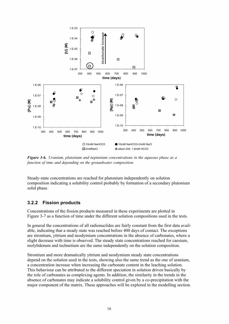
3.2 Radionuclideconcentrationinsolution3.2.1 Actinides

Actinide concentrations in solution as function of time under different contacting solutions are shown in Figure �-6.

The concentrations of the three actinides remain fairly constant in the time interval studied in the present tests, indicating that steady-state was reached within one and a half year and no variation on the concentration of these actinides occurs afterwards. This steady state could be an indication of solubility control in the system. Consequently, thermodynamic approaches are considered to explain the concentrations of the actinides. The exceptions to take into account are uranium and neptunium concentrations in the absence of carbon-ate in the system (grey squares) that show a decrease of the concentration with time. Concentrations of U obtained in the strip solutions were quite remarkable in the absence of carbonates, specifically for the sample indicated with a circle in Figure �-6, since the concentration measured in the strip solution was more than three orders of magnitude larger than the one measured in the leaching solution. This clearly indicates that some sorption or precipitation on the vessel walls occurred in this specific test. The general decrease of neptunium and uranium concentrations with time and in absence of carbonates will be studied later on.

Another important consideration is the different uranium concentrations in the aqueous phase as a function of the solution composition. As we can see in Figure �-6, the higher the carbonate contents in solution the higher the concentration of uranium. This behaviour reflects the strong complexation of uranium with carbonate ligands. Plutonium and neptu-nium concentrations follow the same trend as uranium; this behaviour could be the result of a stronger complexation of these actinides with carbonates combined with a solubility control governed in the case of neptunium by the precipitation of the major element of the matrix, uranium. This possibility will be explored later on.

Figure 3-5.  Hydrogen peroxide concentrations in the aqueous phase as a function of time.

0 10 20 30 40 400 600 800 100010

-8

10-7

10-6

10-5

10-4

CO3

-2 sol., Bruno et al.(1999) allard gw, Bruno et al.(1999)

CO3

-2+Cl - sol., Bruno et al.(2003)

CO3

-2 sol., Bruno et al.(2003) allard gw, this work

CO3

-2+Cl - sol., this work

CO3

-2 sol., this work

Cl - sol., this work

[H2O

2] (

M)

time (days)

16

Steady-state concentrations are reached for plutonium independently on solution composition indicating a solubility control probably by formation of a secondary plutonium solid phase.

3.2.2 Fissionproducts

Concentrations of the fission products measured in these experiments are plotted in Figure �-7 as a function of time under the different solution compositions used in the tests.

In general the concentrations of all radionuclides are fairly constant from the first data avail-able, indicating that a steady state was reached before �00 days of contact. The exceptions are strontium, yttrium and neodymium concentrations in the absence of carbonates, where a slight decrease with time is observed. The steady state concentrations reached for caesium, molybdenum and technetium are the same independently on the solution composition.

Strontium and more dramatically yttrium and neodymium steady state concentrations depend on the solution used in the tests, showing also the same trend as the one of uranium, a concentration increase when increasing the carbonate content in the leaching solution. This behaviour can be attributed to the different speciation in solution driven basically by the role of carbonates as complexing agents. In addition, the similarity in the trends in the absence of carbonates may indicate a solubility control given by a co-precipitation with the major component of the matrix. These approaches will be explored in the modelling section.

Figure 3-6.  Uranium, plutonium and neptunium concentrations in the aqueous phase as a function of time and depending on the groundwater composition.

1.E-07

1.E-06

1.E-05

1.E-04

1.E-03

300 400 500 600 700 800 900 1000

time (days)

[U] (

M)

bica

rbon

ate

incr

ease

1.E-10

1.E-09

1.E-08

1.E-07

1.E-06

300 400 500 600 700 800 900 1000time (days)

[Pu]

(M)

1.E-10

1.E-09

1.E-08

1.E-07

1.E-06

300 400 500 600 700 800 900 1000

time (days)

[Np]

(M)

10mM NaHCO3 10mM NaHCO3+2mM NaCl

2mMNaCl allard GW, 1,8mM HCO3

17

3.2.3 Comparisonwiththepreviousseriesofexperiments.Timeresolvedandlongtermexperiments

Figures �-8 to �-1� show radionuclide concentrations in the aqueous phase gathered since the start of the experimental programme /Bruno et al. 1999, 200�/. Data in the absence of carbonate are not plotted in these figures since these have been discussed in previous subsections.

From data in Figure �-8, we observe a continuous trend of the uranium data generated in the time resolved experiments (short time) and the data obtained from the long time experi-ments; there is an initial increase of the concentration of uranium with time until reaching

Figure 3-7.  Strontium, caesium, molybdenum, technetium, yttrium and neodymium concentrations in the aqueous phase as a function of time and depending on the groundwater composition.

1.E-08

1.E-07

1.E-06

1.E-05

300 400 500 600 700 800 900 1000

time (days)

[Sr]

(M)

1.E-07

1.E-06

1.E-05

1.E-04

300 400 500 600 700 800 900 1000

time (days)

[Cs]

(M)

1.E-07

1.E-06

1.E-05

1.E-04

300 400 500 600 700 800 900 1000

time (days)

[Mo]

(M)

1.E-07

1.E-06

1.E-05

1.E-04

300 400 500 600 700 800 900 1000

time (days)

[Tc]

(M)

1.E-10

1.E-09

1.E-08

1.E-07

300 400 500 600 700 800 900 1000

time (days)

[Y] (

M)

bica

rbon

ate

incr

ease

1.E-10

1.E-09

1.E-08

1.E-07

300 400 500 600 700 800 900 1000

time (days)

[Nd]

(M)

bica

rbon

ate

incr

ease

10 mM NaHCO3 10 mM NaHCO3+2 mM NaCl

2 mM NaCl allard GW, 1,8 mM HCO3

18

a steady state. The same behaviour is observed for neptunium as we can see in Figure �-10. Although, a similar trend is observed for plutonium (see Figure �-9), there is a larger scatter in the data attributed partly to its higher tendency to form colloids. Another possibility would be the fact that different secondary solid phases may control its concentration in the aqueous phase. All these assumptions will be explored in the following sections of this work.

Figure 3-8.  Uranium concentrations in the aqueous phase as a function of time. Open symbols stand for data in carbonate solutions, grey symbols stand for data in carbonate plus chloride solutions and black symbols stand for data in Allard GW.

Figure 3-9.  Plutonium concentrations in the aqueous phase as a function of time. Open symbols stand for data in carbonate solutions, grey symbols stand for data in carbonate plus chloride solutions and black symbols stand for data in Allard GW.

0 10 20 30 40 400 600 800 100010-7

10-6

10-5

10-4

Bruno et al. (1999) Bruno et al. (2003) this work

[U](M

)

time (days)

0 10 20 30 40 400 600 800 1000

10 -9

10 -8

10 -7

10 -6

Bruno et al. (1999) Bruno et al. (2003) this work

[Pu]

(M)

time (days)

19

The same trend as for uranium is observed for strontium, technetium, caesium and molybdenum data when comparing data from the time resolved and long time experiments (see Figures �-11 and �-12): i.e. an increase of radionuclides concentration with time until reaching a steady state after some �0 days.

Figure 3-10.  Neptunium concentrations in the aqueous phase as a function of time. Open symbols stand for data in carbonate solutions, grey symbols stand for data in carbonate plus chloride solutions and black symbols stand for data in Allard GW.

Figure 3-11.  Strontium concentrations in the aqueous phase as a function of time. Open symbols stand for data in carbonate solutions, grey symbols stand for data in carbonate plus chloride solutions and black symbols stand for data in Allard GW.

0 10 20 30 40 400 600 800 1000

10-9

10-8

10-7

10-6

Bruno et al. (1999) Bruno et al. (2003) this work

[Np]

(M)

time (days)

0 10 20 30 40 400 600 800 1000

10-8

10-7

10-6

10-5

Bruno et al. (1999) Bruno et al. (2003) this work

[Sr]

(M)

time (days)

20

Finally, a major scatter is observed in yttrium data, Figure �-1�. Nevertheless, after the initial release period, the concentrations seem to reach a steady state which varies depend-ing on solution composition, as mentioned before. The same applies for neodymium (data not shown).

Figure 3-12.  Technetium concentrations in the aqueous phase as a function of time. Open symbols stand for data in carbonate solutions, grey symbols stand for data in carbonate plus chloride solutions and black symbols stand for data in Allard GW.

Figure 3-13.  Yttrium concentrations in the aqueous phase as a function of time. Open symbols stand for data in carbonate solutions, grey symbols stand for data in carbonate plus chloride solutions and black symbols stand for data in Allard GW.

0 10 20 30 40 400 600 800 100010

-9

10-8

10-7

10-6

10-5

Bruno et al. (1999) Bruno et al. (2003) this work

[Tc]

(M)

time (days)

0 10 20 30 40 400 600 800 1000

10-9

10-8

10-7 Bruno et al. (2003)

this work

[Y](M

)

time (days)

21

4 Datatreatmentanddiscussion

4.1 KineticapproachesforradiolysisproductsThe trends observed in the previous section of results, when comparing hydrogen oxygen and hydrogen peroxide data reported in /Bruno et al. 200�/, with the current one (Figures �-� to �-5), were basically the result of the attainment of different steady states for all the radiolysis products studied. Hydrogen and oxygen concentrations reached the steady state after a continuous increase with time from the beginning of the experiments. On the other hand, for hydrogen peroxide the general trend observed in most of the tests in the short time periods was different, since it was expected an initial increase in the concentration of this compound to reach a maximum value and as the reaction proceeded, the concentration decreased to reach the final steady state. Steady state concentrations were mainly attributed to an overall balance of all the radiolytic species generated in the system. Based on this fact, a kinetic analysis has been done by using experimental data reported in /Bruno et al. 200�/ as well as the data reported in this work corresponding to those tests carried out with bicarbonate in the leaching solution.

The kinetic analysis has been performed macroscopically by considering general processes and consequently the different mechanisms (recombination reactions) taking place for the generation and consumption of these species have not been included in the treatment of the data.

Hydrogen and hydrogen peroxide are formed directly by water radiolysis, with similar radiolytic yields leading to concentrations of these compounds of the same order of magnitude. In addition, these molecular species will be then consumed or generated again by recombination reactions with other compounds or radical species. On the other hand, oxygen will be generated and consumed by several recombination reactions. In order to simplify the system for solving it analytically we have considered that these processes are decoupled, therefore, hydrogen, hydrogen peroxide and oxygen reactions have been treated separately.

4.1.1 Hydrogen

The processes considered for hydrogen are: 1) Generation of hydrogen by water radiolysis:

(�-1)

where k1 (mol×s–1) is the rate of generation.

2) Recombination and consumption of this radiolysis product according to the general reaction:

(�-2)

where k2 (s–1) and k–2 (mol×s–1) are constants the forward and backward reactions in equation �-2 respectively and [H2O2] the hydrogen content in the system.

22

From processes 1 and 2, the variation of hydrogen content with time can be written as:

[ ] [ ]2221

2 HkkkdtHd

×−+= − (�-�)

By integrating this equation, the following expression is obtained for hydrogen content as a function of time:

(�-�)

The fit of this model to the experimental data is shown in Figure �-1, where we may observe that the calculated data reproduces quite well the observed H2(g) generation..

The generation of hydrogen will be dominated by the radiolysis of water and the rate of hydrogen generation will be larger than the rate of formation by the backwards reactions i.e.

k1>>k–2

and consequently may be rewritten as .

From the fit of the model to the experimental data we obtain the rate constants given in Table �-1 for the processes �-1 and �-2.

Figure 4-1.  Moles of hydrogen determined as a function of time. Solid line stands for the fit of the model to the experimental values, according to expression 4-4.

1.E-07

1.E-06

1.E-05

1.E-04

1.0 10.0 100.0 1000.0time(days)

mol

es H

2

exp. data

fitting

2�

4.1.2 Oxygen

Oxygen is not generated directly by water radiolysis, therefore its formation will be given by other processes such as recombination and decomposition reactions. Consequently, we may express the generation and consumption of this compound according to the general process:

(�-5)

where k2 (mol×s–1) and k–2 (s–1) are the constants for the forward and backward reactions respectively. According to this general process, the oxygen content as function of time may be written as:

[ ] [ ]222

2 OkkdtOd

×−= − (�-6)

and the integrated expression by:

(�-7)

The fit of the model to the experimental data is shown in Figure �-2, where we can observe that the calculated function reproduces satisfactorily the observed oxygen generation. The resulting fitting parameters are also given in Table �-1.

Table4-1. Fittedparametersforhydrogenandoxygen.

k1(mol×s–1) k2(s–1) k–2(mol×s–1)

Hydrogen (2.13 ± 0.37)×10–12 (4.49 ± 1.04)×10–8

Oxygen (5.68 ± 2.03)×10–8 (6.79 ± 2.01)×10–13

Figure 4-2.  Moles of oxygen determined as a function of time. Solid line stands for the fit of the model to the experimental values according to expression 4-7. Grey dots correspond to the experimental data used for the model adjustment.

1,E-08

1,E-07

1,E-06

1,E-05

1,E-04

1.0 10.0 100.0 1000.0

time (days)

mol

es O

2

exp. datafitting

2�

4.1.3 Hydrogenperoxide

The time dependence of the hydrogen peroxide concentration in the leach solution (Figure �-5) clearly indicates attainment of steady state after approximately 10 days. Steady state in the first time resolved experiment, starting with dry fuel fragments, was obtained from a low initial peroxide concentration. The initial concentration in following time resolved experiments was, however, > 10–6 M. The reason for this is ascribed to hydrogen peroxide formation on the wet fuel fragment surfaces, not in contact with leach solution, during the process of solution replacement.

The following chain reactions are considered to model the hydrogen peroxide data.1) Generation of hydrogen peroxide by water radiolysis:

(�-8)

where k1 (mol×s–1) is the rate of formation of hydrogen peroxide2) Desorption of the hydrogen peroxide initially present on the moist fuel fragment surfaces

(�-9)

where k2(s–1) is the rate constant of the desorption reaction and > UO2-H2O2 stands for the hydrogen peroxide sorbed on the fuel surface�) Consumption of hydrogen peroxide according to the general reaction:

(�-10)

where k� (s–1) is the rate constant

According to the previous processes, rate equations for hydrogen peroxide and the intermediate product (sorbed hydrogen peroxide) can be expressed as:

(�-11)

(�-12)

The solution of this system of differential equations gives the following expression for the total hydrogen peroxide content in solution as function of time

(�-1�)

where [H2O2] is the hydrogen peroxide content (moles) of the solution and A0 (moles) the initial amount of peroxide sorbed on the fuel surfaces.

The fit of this model to experimental data is given in Figure �-�.

The parameters obtained by this approach, given in Table �-2, are in good agreement with the parameters obtained for hydrogen and oxygen and clearly point at oxygen as the main product formed on decomposition of hydrogen peroxide.

25

Table4-2. Calculatedparametersforhydrogenperoxide.

k1(mol×s–1) k2(s–1) k3(s–1) [H2O2]0(moles)

(1.6 ± 0.20)×10–12 (2.0 ± 0.2)×10–5 (1.64 ± 0.2)×10–4 (2.1 ± 0.50)×10–6

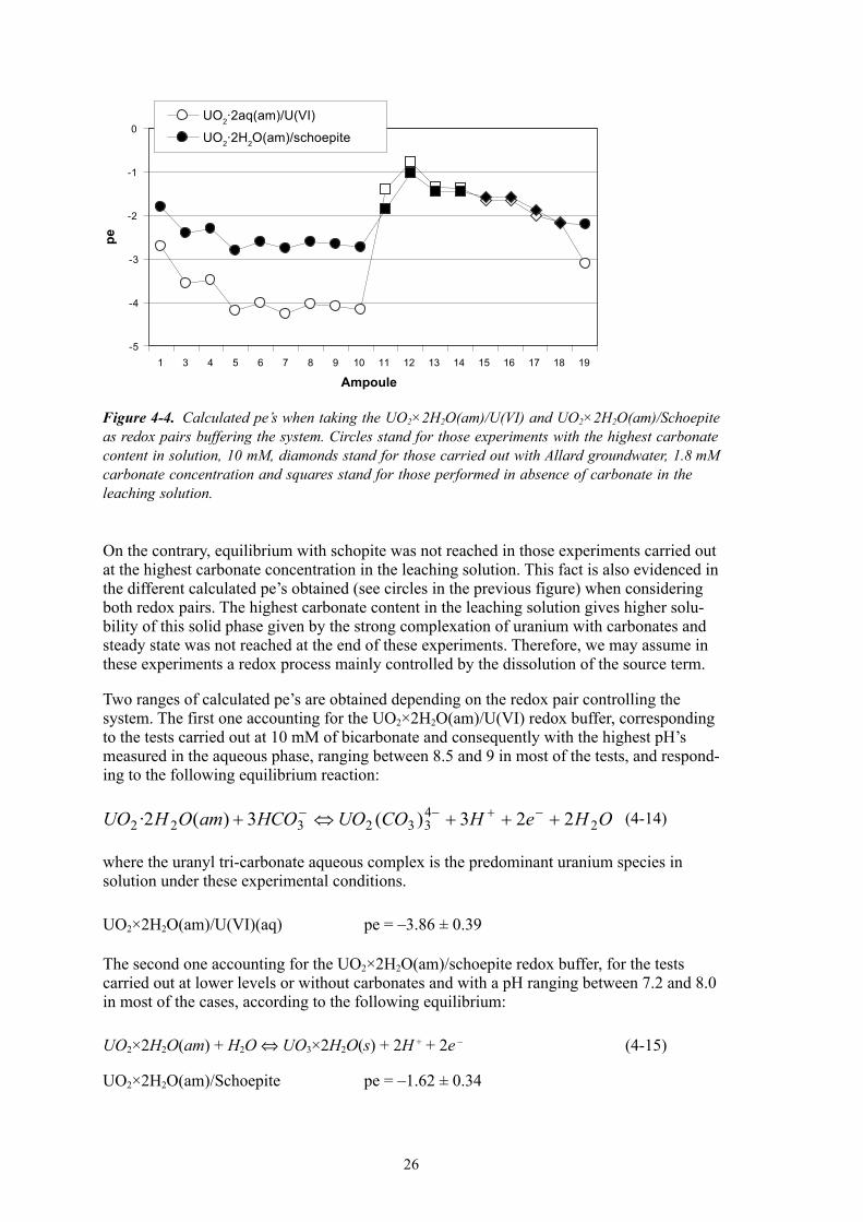
4.2 EstimationoftheredoxconditionsAs it has been stated in the previous works /Eriksen et al. 1995, Bruno et al. 1999, 200�/, oxidant species generated by radiolysis of water oxidize of uranium and other redox sensitive radionuclides present in the fuel sample. The role of the fuel surface in poising the redox state of the heterogeneous systems studied in the previous works has been also largely evidenced and reported in the last years /Casas and Bruno 199�, Bruno et al. 1996/. Therefore, given that experimental conditions reported in the present work are similar to the ones reported in the previous ones, we have once more established the uranium system for defining the redox couple controlling the redox potential in the aqueous phase in the actual series of experiments.

Figure �-2 shows the calculated pe’s when considering the UO2×2H2O(am)/U(VI) as redox pair buffering the system. Saturation indexes evidenced the fact that schoepite should be in equilibrium in those experiments carried out at low concentrations or without carbonate in the aqueous phase. Calculated pe’s when considering the equilibrium UO2×2H2O(am)/Schoepite are also plotted in Figure �-�.

In this figure we can see the agreement in calculated pe’s for those experiments carried out at lower or without carbonate in the system (squares and diamonds symbols in the graph), indicating again that equilibrium with schoepite was attained in these experiments.

Figure 4-3.  Moles of hydrogen peroxide determined as a function of time. Solid line stands for the fit of the model to the experimental values according to expression 4-13. Grey dots correspond to the experimental data used for the fitting of the model.

1.E-09

1.E-08

1.E-07

1.E-06

0.1 1.0 10.0 100.0 1000.0

time (days)

mol

es [H

2O2]

exp. datafitting

26

On the contrary, equilibrium with schopite was not reached in those experiments carried out at the highest carbonate concentration in the leaching solution. This fact is also evidenced in the different calculated pe’s obtained (see circles in the previous figure) when considering both redox pairs. The highest carbonate content in the leaching solution gives higher solu-bility of this solid phase given by the strong complexation of uranium with carbonates and steady state was not reached at the end of these experiments. Therefore, we may assume in these experiments a redox process mainly controlled by the dissolution of the source term.

Two ranges of calculated pe’s are obtained depending on the redox pair controlling the system. The first one accounting for the UO2×2H2O(am)/U(VI) redox buffer, corresponding to the tests carried out at 10 mM of bicarbonate and consequently with the highest pH’s measured in the aqueous phase, ranging between 8.5 and 9 in most of the tests, and respond-ing to the following equilibrium reaction:

(�-1�)

where the uranyl tri-carbonate aqueous complex is the predominant uranium species in solution under these experimental conditions.

UO2×2H2O(am)/U(VI)(aq) pe = –�.86 ± 0.�9

The second one accounting for the UO2×2H2O(am)/schoepite redox buffer, for the tests carried out at lower levels or without carbonates and with a pH ranging between 7.2 and 8.0 in most of the cases, according to the following equilibrium:

UO2×2H2O(am) + H2O ⇔ UO�×2H2O(s) + 2H + + 2e – (�-15)

UO2×2H2O(am)/Schoepite pe = –1.62 ± 0.��

Figure 4-4.  Calculated pe’s when taking the UO2×2H2O(am)/U(VI) and UO2×2H2O(am)/Schoepite as redox pairs buffering the system. Circles stand for those experiments with the highest carbonate content in solution, 10 mM, diamonds stand for those carried out with Allard groundwater, 1.8 mM carbonate concentration and squares stand for those performed in absence of carbonate in the leaching solution.

-5

-4

-3

-2

-1

0

1 3 4 5 6 7 8 9 10 11 12 13 14 15 16 17 18 19

Ampoule

peUO2·2aq(am)/U(VI)

UO2·2H2O(am)/schoepite

27

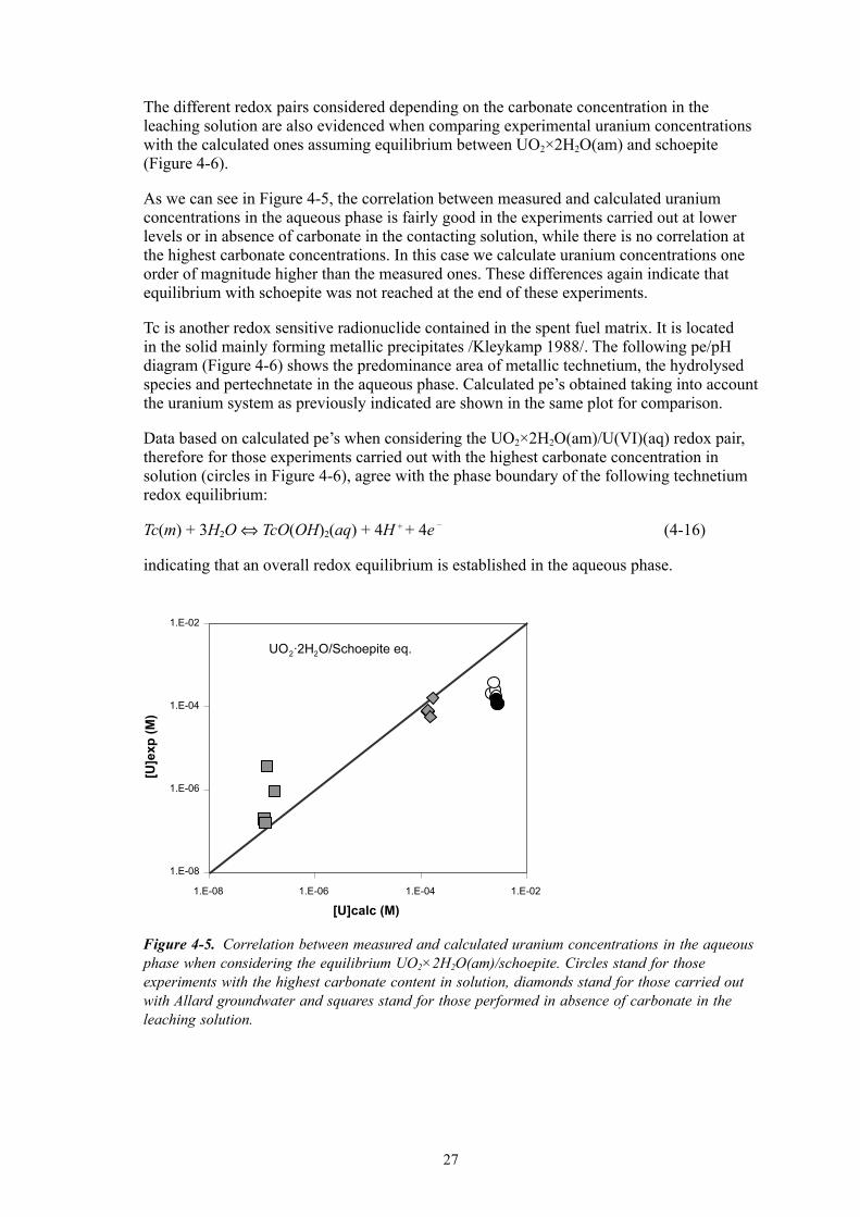
The different redox pairs considered depending on the carbonate concentration in the leaching solution are also evidenced when comparing experimental uranium concentrations with the calculated ones assuming equilibrium between UO2×2H2O(am) and schoepite (Figure �-6).

As we can see in Figure �-5, the correlation between measured and calculated uranium concentrations in the aqueous phase is fairly good in the experiments carried out at lower levels or in absence of carbonate in the contacting solution, while there is no correlation at the highest carbonate concentrations. In this case we calculate uranium concentrations one order of magnitude higher than the measured ones. These differences again indicate that equilibrium with schoepite was not reached at the end of these experiments.

Tc is another redox sensitive radionuclide contained in the spent fuel matrix. It is located in the solid mainly forming metallic precipitates /Kleykamp 1988/. The following pe/pH diagram (Figure �-6) shows the predominance area of metallic technetium, the hydrolysed species and pertechnetate in the aqueous phase. Calculated pe’s obtained taking into account the uranium system as previously indicated are shown in the same plot for comparison.

Data based on calculated pe’s when considering the UO2×2H2O(am)/U(VI)(aq) redox pair, therefore for those experiments carried out with the highest carbonate concentration in solution (circles in Figure �-6), agree with the phase boundary of the following technetium redox equilibrium:

Tc(m) + �H2O ⇔ TcO(OH)2(aq) + �H + + �e – (�-16)

indicating that an overall redox equilibrium is established in the aqueous phase.

Figure 4-5.  Correlation between measured and calculated uranium concentrations in the aqueous phase when considering the equilibrium UO2×2H2O(am)/schoepite. Circles stand for those experiments with the highest carbonate content in solution, diamonds stand for those carried out with Allard groundwater and squares stand for those performed in absence of carbonate in the leaching solution.

UO2·2H2O/Schoepite eq.

1.E-08

1.E-06

1.E-04

1.E-02

1.E-08 1.E-06 1.E-04 1.E-02

[U]calc (M)

[U]e

xp (M

)

28

On the other hand, calculated pe’s by taking the UO2×2H2O(am)/schoepite system (diamonds and squares in Figure �-6), leading to higher redox potentials in the aqueous phase, indicate that probably the Tc system established in these experiments is governed by the following equilibrium in the aqueous phase:

TcO(OH)2(aq) + H2O ⇔ TcO4–

+ �H + + �e –

(�-17)

The disagreement between data points and phase boundaries may, however, indicate kinetic control.

4.3 Thermodynamicandkineticapproachesforradionuclidesrelease

4.3.1 Testscarriedoutwithahighercarbonatecontentintheleachingsolution

According to the general trend observed in the previous section of results when comparing data reported in /Bruno et al. 200�/, with the present data (Section �.2.�), we can establish for most of the trace elements studied a general behaviour corresponding to an increase of the concentration in solution when the solid is put in contact with the aqueous phase until attaining a steady state. Based on this fact, kinetic and thermodynamic analyses have been carried out using experimental data reported in /Bruno et al. 200�/ for the experiments carried out without sodium chloride and with 1 mM of sodium chloride in the leaching solution as well as the data reported in this work corresponding to the tests carried out with 10 mM bicarbonate in the leaching solution, with and without sodium chloride (Ampoules 1 to 10 and 19).

To do this, based on the thermodynamic analysis carried out in /Bruno et al. 200�/ and according to the results obtained in the new series of experiments presented in this work (see Section �.2), we have assumed congruent release of most of the trace elements studied with the spent fuel matrix, uranium. The only exceptions are Pu, Y and Nd as we will see in the following sub-sections.

Figure 4-6.  pe/pH diagram showing the predominance of Tc species (black lines), [Tc]aq = 10–

6 M. Squares, diamonds and circles stand for pe/pH data values with pe’s based on the calculated values when considering the uranium systems (see text).

-5.0

-3.0

-1.0

1.0

3.0

7 7.5 8 8.5 9 9.5

pH

pe

Tc(cr)

TcO(OH)2(aq)

TcO4-

29

4.3.1.1U

As given in Figure �-8, uranium concentrations in the aqueous phase show a constant increase with time until reaching a steady-state. This steady-state level does not agree with the formation of any secondary solid phase, so, as previously reported, this steady state is controlled by matrix dissolution.

Therefore, the kinetic modelling has been performed for the major component of the matrix, U, based on the previous equilibrium reaction (�-1�):

OHeHCOUOHCOamOHUO2

4

332322223)(3)(2× +++⇔+ −+−−

k-1

k1

(�-1�)

where the uranyl tri-carbonate aqueous complex is the predominant uranium species in solution under these experimental conditions (for the sake of simplicity we will refer to this complex as U(VI)). Consequently the generation of uranium in the aqueous phase with time can be expressed as:

(�-18)

where k1 is the forward rate, including the term of [HCO�–]� which is considered to be

constant and k–1 is the constant for the backward reaction, including the terms [H+]� × [e–]2 that are also considered constant terms under the actual conditions.

Therefore, by integration of this equation we obtain the following expression for uranium concentration as a function of time:

(�-19)

The fit of equation �-19 to the experimental data is given in Figure �-7. The adjusted parameters are shown in Table �-�.

Figure 4-7.  Data points stand for measured uranium concentrations as a function of time. Solid line stands for the fit of the model to the experimental values, according to the expression 4-19.

1.0E-07

1.0E-06

1.0E-05

1.0E-04

1.0E-03

1 10 100 1000

time (days)

[U] (

M)

exper. data

fitting

�0

Table4-3. Fittedparametersforuraniumdissolution,accordingtoreaction4-14andequation4-19.

Uranium

k1 (2.64 ± 0.02)×10–6 M/dk–1 (1.65 ± 0.22)×10–2 d–1

Based on the principle of detailed balancing /Lasaga et al. 1981/, we can correlate the kinetic rate constants obtained from the fitting of the data to the thermodynamic constant for reaction �-1�, according to the following expression:

(�-20)

where , and Ks stands for the solubility constant of reaction �-1�.

By using the parameters obtained in the non-linear least square fitting we calculate a log Ks value of –16.77 ± 0.06 which is very close to the thermodynamic parameter, log Ks = –16.81 ± 1.76 /Grenthe et al. 1992/ for the same reaction. This agreement gives an inde-pendent confirmation on the results obtained from the modelling exercise and consequently on the validity of the processes considered.

By rewriting the previous expression �-19 by substitution of k+ according to equation �-20, we obtain a general rate expression that is a linear relation with the coefficient Q/Ks, that is, the affinity, where Q is the activity product and Ks is the solubility constant:

(�-21)

Figure �-8 is a plot showing the relation between the dissolution rates and the affinity, as expected we have an initial linear ratio between the dissolution rate and the affinity, it means, far from equilibrium, however, as the reaction proceeds, this relation is decreas-ing until having a constant release rate close to zero when approaching equilibrium. The horizontal trend showed in Figure �-8 at very low affinities indicates that concentrations close to equilibrium are attained very fast, see Figure �-8 for checking.

The dissolution rates calculated in this work as well as other values reported in the literature are given in Table �-�. Dissolution rates are compared directly for those experiments carried out under similar experimental conditions or calculated based on rate equations reported in the literature. The value determined in this work is in most of the cases lower than the ones reported in previous work. However, this is an expected result taking into account that oxygen concentrations in the actual work were much lower than the ones of the experiments carried out under oxidising conditions (at least two orders of magnitude). On the other hand, when comparing with the range of dissolution rates obtained by using the rate equation reported in /de Pablo et al. 1999/, these values are lower than the one reported in the present work. This discrepancy was also observed when /de Pablo et al. 1999/ tried to predict the rates of dissolution of spent fuel measured by /Gray and Wilson 1995/ and, as the authors pointed out, the possibility of other oxidants besides O2 generated by radiolysis actively oxidising the spent fuel would surely account for this discrepancy.

�1

Table4-4. ComparisonofinitialdissolutionratesforunirradiatedUO2andspentfuelundersimilarexperimentalconditions.

Sampletype Rateequations Redoxcond r(mole×m–2×s–1)

/Gray et al. 1992/ Spent fuel oxidising 1.38×10–10

/Gray et al. 1992/ Spent fuel r = f(T, pH,T,[Ctot]) oxidising 6.07×10–10

/de Pablo et al. 1997/ Unirradiated UO2 r = f(T,[HCO3]) oxidising 1.07×10–10

/de Pablo et al. 1999/ Unirradiated UO2 r = f([O2],[HCO3]) 8.89×10–15–1.77×10–12

/Röllin et al. 2001/ Spent fuel r = f(pH,[HCO3]) oxidising 2.13×10–10

This study Spent fuel anoxic 5.59×10–11

4.3.1.2CsandSr

Figure �-11 shows the general trend of strontium data with time. However, the steady state values do not agree with the solubility of any secondary solid phase able to precipitate under the experimental conditions of these tests. Strontium and caesium are very soluble radionuclides under these experimental conditions and they are not solubility limited. This trend indicates that Sr releases with matrix dissolution, so when matrix dissolution decreases, Sr release also decreases with time. Based on this behaviour and taking into account that the trend for caesium is the same; kinetic modelling has been based on the following general reaction:

( ) +⇔ 2

2)(', RnsOsRnU

k1

k-1

(�-22)

where k1 and k–1 stand for the forward and backward rate constants respectively. k1 in these cases has been fixed based on a congruent release of these radionuclides with the major component of the fuel matrix and according to the following reaction:

k1 (Rn) = χ Rn × k1(U) (�-2�)

where χ is the fraction of inventory for the given radionuclide.

Figure 4-8.  Uranium dissolution rates as a function of the affinity.

0.E+00

1.E-07

2.E-07

3.E-07

4.E-07

5.E-07

6.E-07

0.00 0.02 0.04 0.06 0.08

Affinity (Q/K)

r (m

ole/

d·m

2)

experimental scatter in dataexpected trend

�2

According to reaction �-10 the generation of these radionuclides in the aqueous phase with time can be expressed as:

[ ] [ ]+−−= (�-2�)

Proceeding as in the previous case, we obtain the following expression for the concentration of these radionuclides as a function of time:

[ ] ( )×−−×= −−

(�-25)

with k1 as a known parameter, and k–1 the rate constant to be fitted with experimental data. The results of these calculations are given in Figure �-9 and Table �-5.

The fit of the model to the experimental data is fairly good for both radionuclides. The modelling gives confidence on the processes previously stated, strontium and caesium release congruently with the spent fuel matrix and their release rate decreases accordingly as the dissolution of the matrix proceeds.

Table4-5. Calculatedandfittedparametersforstrontiumandcaesiumrelease,accordingtoequations4-23and4-25respectively.

k1(calculated) k–1(fitted)

Strontium (7.10 ± 0.84)×10–9 M/d (1.10 ± 0.04)×10–2 d–1

Caesium (1.64 ± 0.22)×10–8 M/d (7.10 ± 1.80)×10–4 d–1

Figure 4-9.  Left and right graphs show measured strontium and caesium concentrations in the aqueous phase respectively as a function of time. Solid lines stand for the fit of the model to the experimental values, according to the expression 4-25.

1.0E-09

1.0E-08

1.0E-07

1.0E-06

1.0E-05

1 10 100 1000

time(days)

[Sr]

(M)

exper. data

fitting

1.0E-08

1.0E-07

1.0E-06

1.0E-05

1.0E-04

1 10 100 1000

time(days)

[Cs]

(M)

exper. datafitting

��

4.3.1.3TcandMo

Figure �-12 is a plot of technetium concentrations as a function of the contact time, the general trend is also observed for this radionuclide. According to the previous modelling to estimate the redox conditions of these tests we assume dissolution of technetium to the aqueous phase governed by the release of the metallic particles located in the fuel samples according to the following reaction:

−+ ++⇔+ (�-16)

where k1 and k–1 stand for the forward and backward rate constants respectively.

Therefore, proceeding as in the uranium case, we obtain for the technetium concentration in the aqueous phase as a function of time as the following expression:

[ ] ( )×−−×= −−

(�-26)

Based on the results obtained in /Bruno et al. 200�/ where a co-dissolution process of this element with the fuel matrix was established, we assume congruency. Therefore as in the cases of strontium and caesium, k1 has been fixed for the fitting of the model to the experi-mental data and calculated according to equation �-26.

The results are given in Figure �-10 and Table �-6.

Table4-6. Calculatedandfittedparametersfortechnetiumdissolution,accordingtoequations4-23and4-26respectively.

Technetium

k1 (calculated) (6.57 ± 0.97)×10–9 M/dk–1 (fitted) (6.06 ± 0.57)×10–3 d–1

Figure 4-10.  Measured technetium concentrations in the aqueous phase as a function of time. Solid line stands for the fit of the model to the experimental values, according to the expression 4-26.

1.E-09

1.E-08

1.E-07

1.E-06

1.E-05

1 10 100 1000

time(days)

[Tc]

(M)

exper. datafitting

��

Based on the principle of detailed balancing and proceeding as in the case of uranium, we have also correlated the kinetic parameters with the thermodynamic one for the previous reaction �-16. The log Ks calculated by using the kinetic parameters from Table �-6 is –26.12 ± 0.08, comparable to the thermodynamic solubility constant reported for this reaction, logKs = –25.08 ± 1.55 /Rard et al. 1999/. This agreement gives again confidence on the results obtained from the modelling exercise and consequently on the validity of the processes considered.

The trend observed for molybdenum release as previously stated is the same as technetium. Mo is not solubility limited given mainly by the formation of MoO�

– in the aqueous phase as a result of the oxidants present in the spent fuel/water interface. As previously reported /Bruno et al. 200�/, Mo can be found in the spent fuel forming metallic particles or oxide precipitates, therefore, assuming the last form, its kinetics of dissolution may be expressed as follows:

(�-27)

Proceeding as before, we obtain:

[ ] ( )×−−×= −−

− (�-28)

k1 has been also set fix for the fitting of the model to the experimental data based on a congruent release of this radionuclide with the fuel matrix, and therefore, calculated accord-ing to equation �-2�. However, in this case, based on the previous modelling done /Bruno et al. 200�/, we have considered two fractions for calculating this rate constant, the first one corresponding to the fuel inventory (χ = 1.01 ± 0.17)×10–2), and the second one correspond-ing to the fraction in solution (χ = 1.58 ± 0.01)×10–2), reported in /Bruno et al. 200�/, that is slightly higher than the one corresponding to the inventory. /Bruno et al. 200�/ explained the highest Mo release with respect to the fraction of the inventory based on the highest affinity for oxygen than Tc. The results of both fittings are shown in Figure �-11.

Figure 4-11.  Measured molybdenum concentrations in the aqueous phase as a function of time. Solid line stands for the fit of the model to the experimental values assuming congruency according to the inventory. Dotted line stands for the fit of the model to the experimental data assuming a larger Mo release than the one expected according to the inventory (see text).

1.0E-08

1.0E-07

1.0E-06

1.0E-05

1.0E-04

1 10 100 1000

time(days)

[Mo]

(M)

exper. datafitting, invent. ratiofitting, aq. ratio

�5

Table4-7. Calculatedandfittedparametersformolybdenumdissolution,accordingtoequations4-23and4-28respectively.

Molybdenum

k1 (calculated) (4.17 ± 0.03)×10–8 M/dk–1 (fitted) (6.42 ± 0.13)×10–3 d–1

Figure �-11 shows the best adjustment of the model to the data assuming a co-dissolution process with the spent fuel matrix, considering a slightly larger release than the one based on the inventory. Calculated and fitted parameters, considering the best model are given in Table �-7.

4.3.1.4Np

The analysis of the primary data, Figure �-10, indicates that neptunium follows the same trend as uranium. According to the analysis carried out before /Bruno et al. 200�/, we may expect a congruent release of this radionuclide with the spent fuel matrix according to the inventory of the fuel sample. On the other hand, Np concentrations in the long time tests reported in the present work, seem to attain a steady state corresponding to the precipitation of a secondary solid phase, Np(OH)�(s). Consequently, in order to proceed with the kinetic analysis of the data, we considered the following processes:1) Release of Np from the spent fuel matrix, according to the following reaction:

( ) ⇒+ (�-29)

where Np(OH)�(aq) is the predominant aqueous species under these experimental condi-tions and k1 is the forward rate constant.

The back reaction is neglected in this case given the subsequent precipitation as a secondary solid phase.2) Np(OH)�(s) precipitation from the dissolved Np(IV) species, according to this reaction:

⇔ (�-�0)

where k2 and k–2 are the forward and backward rate constants respectively.

From both processes, the variation of Np concentrations with time can be written as:

[ ] [ ]×−+= − (�-�1)

By integrating this expression, the following expression for the neptunium concentration as a function of time is obtained:

[ ] ( )×−−×+= − (�-�2)

�6

The fit of the model to the experimental data is shown in Figure �-1�, where we may observe the good agreement between them. By assuming the congruent release with the spent fuel matrix, from the fitting parameters we obtain that k–2 is close to zero, and there-fore the back reaction of the precipitation process can be considered negligible in the actual experiments. Calculated and fitting parameters are also given in Table �-8.

On the other hand, the same graph shows calculated solubilities of the solid phase expected to precipitate by considering two different thermodynamic constants reported in the litera-ture. Concerning the thermodynamic constraints, although the solubility constant reported by /Neck and Kim 2001/ with a log Ks = –0.7 for the reaction Np(OH)�(s) = Np�++2H2O is the one recommended by the NEA-TDB, we may observe in Figure �-12 that the solubility of this amorphous solid phase fits much better when considering a log Ks value correspond-ing to a slightly less crystalline solid phase, as the one reported in the NAGRA database /Pearson et al. 1992/, with logKs = 0.81 for the same reaction.

Table4-8. Calculatedandfittedparametersforneptuniumdissolutionandprecipita-tion,accordingtoequations4-23and4-32respectively.

Neptunium

k1 (calculated) (1.22 ± 0.25)×10–9 M/dk2 (fitted) (3.64 ± 0.21)×10–2 d–1

Figure 4-12.  Measured neptunium concentrations in the aqueous phase as a function of time. Solid line stands for the fit of the model to the experimental values, according to the expression 4-32. Dotted lines correspond to Np(OH)4(s) solubility under these experimental conditions for two reported thermodynamic constants, /Neck and Kim 2001/, with a logKs = –0.7 and /Pearson et al. 1992/ with a logKs = 0.81.

1.E-10

1.E-09

1.E-08

1.E-07

1 10 100 1000time(days)

[Np]

(M)

exper. data

fitting

Neck & Kim (2001)solub.Pearson et al.(1992) solub.

�7

4.3.1.1Pu

As it has been noticed in the analysis of the results (Figure �-9) and in /Bruno et al. 200�/, measured Pu concentrations in the aqueous phase suggest that additional mechanisms to the matrix dissolution, mainly the precipitation of secondary solid phases govern the overall behaviour of this radionuclide in the aqueous phase. This is mainly due to the high stability of the Pu secondary solid phases able to precipitate, that lead to Pu steady state concentrations at very short contact times of the spent fuel with the leaching solution. Given this premise, the modelling of plutonium data has been only based on a thermodynamic approach.

Although the scatter of values, two different ranges of Pu concentrations may be observed in Figure �-1�, the first range corresponding to Pu concentrations measured in the time resolved experiments /Bruno et al. 200�/ and the second one corresponding to the ones reported in the actual work for the long time experiments. This is an indication that different solid phases should control the Pu concentrations in the aqueous phase.

As previously stated, the main process controlling the redox conditions in these tests is the dissolution of the matrix, so the redox buffer will be given by the UO2×2H2O(am)/U(VI)(aq). Calculated pe’s by assuming this redox pair in front of pH are plotted in Figure �-1� that is a predominance diagram of Pu aqueous complexes. From the diagram we may observe that while pe/pH data reported in the previous work /Bruno et al. 200�/ fall in the predominance area of Pu(IV) (open points), where Pu(OH)�(aq) is the predominant aqueous species under these experimental conditions, the data reported in the present work (solid points) fall in the Pu(III)/Pu(IV) phase boundary, indicating that a reduction of Pu(IV) to Pu(III) can take place in these tests.

Based on the different aqueous speciation that should be present in these tests, basically depending on the time, the thermodynamic modelling has been conducted on studying the different Pu(III) and Pu(IV) solid phases able to precipitate under these experimental conditions. The results of this modelling exercise are given in Figure �-15.

The previous figure shows the agreement of Pu concentrations measured in the time resolved experiments (open points) with the solubility curve of Pu(OH)�(am) as stated in the previous work /Bruno et al. 200�/. On the other hand, the ones measured at longer time spans (solid points) are closer to saturation with respect to the mixed PuOHCO�(s) phase. These results show how the redox system and consequently the redox conditions of these tests may act on redox sensitive elements like Pu.

Figure 4-13.  Measured plutonium concentrations in the aqueous phase as a function of time.

1.E-10

1.E-09

1.E-08

1.E-07

1.E-06

0.01 0.1 1 10 100 1000

time (days)

[Pu]

(M)

this workBruno et al., 2003

�8

4.3.1.2YandNd

According to the modelling performed in /Bruno et al. 200�/, no conclusions were drawn about the processes controlling the release of these radionuclides from the fuel. The unexpected non congruent release of these elements with the fuel matrix as well as the fact that we would not expect their co-precipitation with uranium since as we have previously seen the release of uranium in these experiments is only controlled by the oxidative dissolution of the matrix without precipitation of any secondary solid phase, lead us to think of a solubility control given by the precipitation of a secondary solid phase.

Given that in the current tests we can expect the presence of Pu(III) in the system, we have related this radioelement with Y and Nd. For that we have first compared the Pu concentra-tions obtained in both series of tests with the ones of Y and Nd. This comparison is given in Figure �-16.

Figure 4-14.  pe/pH diagram showing the predominance of Pu species (black lines). White circles stand for data reported in /Bruno et al. 2003/, Black circles stand for data reported in this work. Total carbonate concentration, 10 mM.

Figure 4-15.  Solubility curves for Pu(OH)4(am) and PuOHCO3(s) as a function of pe. Data points stand for measured Pu concentrations in the aqueous phase.

-6

-5

-4

-3

-2

-1

7.5 8 8.5 9 9.5

pH

pe

Pu(CO3)2-

Pu(CO3 )2 (OH)2

2-

Pu(CO3)33-

-10.0

-9.0

-8.0

-7.0

-6.0

-5.0

-4.0

-5.0 -4.0 -3.0 -2.0pe

log[

Pu]

(M)

PuOHCO3(s)Pu(OH)4(am)

�9

Y and Nd data fall in the same range of concentrations as Pu both in the time resolved and the long time experiments. Considering that in the present experiments a Pu(III) solid phase seems to control Pu concentrations in the aqueous phase, we can also consider these mixed solid phases for Y and Nd. Given that no thermodynamic data are reported in the literature for YOHCO�(s), its logK value has been obtained by correlation, logK versus q/r. The results of this modelling approach are given in Figure �-17.

Nd concentrations measured in the long time experiments (this work) agree fairly well with the NdOHCO� solubility curve, while Y concentrations are around a half order of magnitude lower than YOHCO� solubility. So, these results seem to indicate that in the long time experiments we should expect a solubility control given by these solid phases. However, we do not have enough evidences to establish the mechanisms controlling the release of these elements in these experiments.

Figure 4-16.  Measured plutonium, yttrium and neodymium concentrations in the aqueous phase as a function of time.

Figure 4-17.  Solubility curves for NdOHCO3(s) and YOHCO3(s) as a function of pH. Data points stand for measured concentrations in the aqueous phase (see legend).

1.E-10

1.E-09

1.E-08

1.E-07

1.E-06

0.01 0.1 1 10 100 1000

time (days)

[Rn]

(M)

Pu, this workPu (Bruno et al., 2003)Y, this workY (Bruno et al., 2003)Nd, this workNd (Bruno et al., 2003)

-10.0

-9.0

-8.0

-7.0

-6.0

-5.0

7.5 8.0 8.5 9.0 9.5

pH

log[

Rn]

(M)

[Y]exp., this work[Y]exp., Bruno et al., 2003YOHCO3(s)[Nd]exp., this work[Nd]exp., Bruno et al., 2003NdOHCO3(s)

�0

4.3.2 Testscarriedoutwithalowconcentrationorwithoutcarbonatesintheleachingsolution

No short term data under low carbonate concentration or without carbonates are currently available. Therefore, only thermodynamic modelling has been conducted in these condi-tions.

4.3.2.1U

As stated before, the concentration of uranium in the aqueous phase in these series of experiments carried out at low concentrations or without carbonate in the leaching solution was limited by the precipitation of schoepite. Therefore, we may establish the following sequence of processes:1) Oxidation of the surface of the fuel sample, and release of uranium as U(VI) to the

solution:

UO2×2H2O(am) ⇔ UO2 (OH)2(aq) + 2H + + 2e – (�-��)

where UO2(OH)2(aq) is the predominant aqueous species in those tests carried out in sodium chloride solution, so, in the absence of carbonates in the system, and

2UO2×2H2O(am) + HCO�– ⇔ (UO2)2(OH)�CO�

– + �H + + �e – + H2O (�-��)

with (UO2)2(OH)�(CO�)– the predominant aqueous species in those tests performed with Allard ground water (1.8 mM HCO�

–).2) Precipitation of a secondary solid phase, schoepite:

UO2 (OH)2(aq) + H2O ⇔ UO� × 2H2O(s) (�-�5)

for those experiments carried out with a sodium chloride solution, and

(UO2)2(OH)�CO�– + �H2O ⇔ 2UO� × 2H2O(s) + HCO�

– (�-�6)

for the ones performed in Allard ground water.

The agreement between U concentrations measured in the aqueous phase and the solubility curves of schoepite in both media is shown in Figure �-18. This agreement gives confidence to the estimation of the redox processes controlling the systems under study and at the same time confirm this secondary solid phase as responsible of the solubility control for the major component of the fuel sample.

It is important to notice the evolution of U concentrations in both series as a function of time (Figure �-19). In Allard ground water, U concentrations reached a steady-state after one year and afterward remained constant with time. This trend denotes that the concentra-tion of this radionuclide increased with time until attaining equilibrium with schoepite. On the contrary, in the tests carried out with a sodium chloride solution, a decrease of the U concentrations in the aqueous phase with time was observed, indicating that the precipita-tion process was taking place from an oversaturated state.

�1

4.3.2.1Sr,Cs,MoandTc

As stated in the previous treatment of the data and according to calculation of the satura-tion indexes for the solid phases able to precipitate, strontium, caesium, molybdenum and technetium are very soluble radionuclides under the experimental conditions of the actual tests and consequently they will not be solubility limited. Therefore, according to the gen-eral trend of the experimental data showed in the section of results and also in agreement with the previous modelling, we might expect a release of these radionuclides controlled by the matrix dissolution. Concentrations measured in Allard groundwater are in general larger than the ones measured in sodium chloride for all the fission products studied in this section, since the major dissolution of the matrix due to the stronger U complexation with carbonates leads to a major release of the radionuclides associated to it. On the other hand, the decrease in the concentration of the major component of the fuel matrix leads to steady-state concentrations for these radionuclides given that the dissolution of the matrix does not proceed in these tests. These diverse behaviours are also depicted in Figure �-20, showing the normalised concentrations of these radionuclides with respect to U as a function of time.

Figure 4-18.  Solubility curves for schoepite (UO3×2H2O(s)) as a function of pH. Data points stand for measured U concentrations in the aqueous phase. Left: data in Allard gw. Right: data in a sodium chloride solution.

Figure 4-19.  Measured uranium concentrations in the aqueous phase as a function of time.

1.E-06

1.E-05

1.E-04

1.E-03

1.E-02

6 7 8 9 10

pH

[U] (

M)

exper. datape = -2pe = -1

Allard gw

1.E-08

1.E-07

1.E-06

1.E-05

1.E-04

1.E-03

6 7 8 9 10pH

[U] (

M)

exper. datape = -2pe = -1

NaCl sol.

1.E-08

1.E-07

1.E-06

1.E-05

1.E-04

1.E-03

300 400 500 600 700 800 900 1000

time (days)

[U] (

M)

NaCl sol.

Allard gw

�2

Normalised concentrations with respect to U are kept constant in those tests performed in Allard groundwater, indicating once again a fission products release in agreement with matrix dissolution. On the other hand, normalised concentrations increase with time in those tests carried out with a leaching solution containing sodium chloride. The decrease in the uranium concentrations with time leads to an increase in this ratio as the precipitation reaction proceeds. Therefore, we may establish a congruent release but an incongruent precipitation.

4.3.2.2PuandNp

As we have previously stated (Figure �-9), measured Pu concentrations in the aqueous phase for these series of tests suggest that again the precipitation of a secondary solid phase governs Pu concentrations in the aqueous phase. As previously noticed, this is basically due to the high stability of the Pu secondary solid phases able to precipitate, that lead to Pu steady state concentrations at very short contact times. The range of Pu concentrations measured in these tests is the same independently on the leaching solution. This behaviour indicates that, first, we can not establish any congruency in its release with the matrix and second, we may expect the precipitation of the same secondary solid phase with no depend-ence on the contacting solution.

Pu in the aqueous phase is expected to be predominantly in the form of Pu(IV) aqueous species in both leaching solutions as we observe in Figure �-21. Based on these results, Pu(OH)�(s) has been taken as the solid phase able to precipitate in the present conditions. The results of the thermodynamic modelling are given in Figure �-22.

As we can see in Figure �-22, measured data fall within the limits of the solubility curves of Pu(OH)�(am), indicating that we may expect the precipitation of this secondary solid phase in the actual conditions of these series of tests.

The analysis of the primary Np data, Figure �-2�, indicates that neptunium follows the same trend as uranium. In Allard ground water U, as well as Np concentrations slightly increase with time, while in NaCl solution, we observe for both elements the opposite effect. These similarities agree once again with the previous modelling, with the establishment of a co-dissolution process to explain Np release.

Figure 4-20.  Normalised Rn concentrations with respect to U. Left hand, experimental data taken from tests performed in Allard groundwater. Right hand, experimental data from tests performed in sodium chloride solutions.

1.E-03

1.E-02

1.E-01

1.E+00

400 500 600 700 800 900 1000

time(days)

Nor

mal

ised

to U

Sr aq. Cs aq.

Tc aq. Mo aq.

Allard gw

1.E-02

1.E-01

1.E+00

1.E+01

1.E+02

350 450 550 650 750 850 950

time(days)

Nor

mal

ised

to U

Sr aq. Cs aq.

Tc aq. Mo aq.

NaCl sol.

��

Figure �-2� is a plot of measured Np concentrations as a function of pH. The same plot contains the solubility curve of Np(OH)�(s), which is the solid phase expected to precipitate under these conditions. As we can see, in this graph, Np concentrations measured in Allard groundwater fall in the solubility curve of Np(OH)�(s), while the ones measured in the NaCl solution are undersaturated with respect to this solid phase.

The larger release of U in Allard groundwater leads to a larger release of Np according to congruency as stated in the previous modelling exercise, reaching a steady-state correspond-ing to the precipitation of a secondary solid phase, Np(OH)�(s).

Figure 4-21.  pe/pH diagrams showing the predominance of Pu species (black lines) Left: predominance diagram in Allard gw. Right: predominance diagram in a sodium chloride solution. Circles stand for data reported in this work, pe calculated by taking UO2×2H2O/schoepite redox pair.

Figure 4-22.  Solubility curves for Pu(OH)4(am) as a function of pH (solid lines). Dotted lines indicate the error bars associated to the logKs = –0.8 ± 1.3 /Lemire and Garisto 1989/. Data points stand for measured Pu concentrations in the aqueous phase (see legend).

-3

-2.5

-2

-1.5

-1

-0.5

0

0.5

1

6 6.5 7 7.5 8 8.5

pH

pe

PuCO3+

Pu(OH)4(aq)

-3

-2.5

-2

-1.5

-1

-0.5

0

0.5

1

6 6.5 7 7.5 8 8.5

pH

pe

Pu3+

Pu(OH)4(aq)

PuOH2+

1.E-10

1.E-09

1.E-08

1.E-07

1.E-06

1.E-05

1.E-04

6 7 8 9 10

pH

[Pu]

(M)

Pu exp., Allard gw

Pu exp., NaCl sol.

Pu(OH)4(s), Allard gw

Pu(OH)4(s), NaCl sol.

��

On the other hand, in those tests carried out without carbonates in the leaching solution, the dissolution of U has been slower, and so is the Np release. In such cases, no equilibrium with any Np secondary solid phase has been attained. The decrease in Np concentrations with time in agreement with U decrease lead us to think in a co-precipitation of Np with the uranium secondary solid phase, schoepite. The incorporation of Np in U(VI) compounds has been reported in other studies /Buck et al. 1998, Finch et al. 2002/. These authors propose a Np solubility model based on a Np-bearing schoepite as the solid phase limiting dissolved Np concentrations. Although no enough data are available to establish this mecha-nism in the present tests, given the general trend observed for Np data a similar mechanism cannot be discarded.

Figure 4-23.  Measured uranium and neptunium concentrations in the aqueous phase as a function of time. Arrows indicate the trends as explained in the text.

Figure 4-24.  Solubility curve for Np(OH)4(am) as a function of pH (solid line). Data points stand for measured Np concentrations in the aqueous phase (see legend). The arrow indicates time evolution of Np concentrations in NaCl solutions.

1.E-10

1.E-09

1.E-08

1.E-07

1.E-06

1.E-05

1.E-04

1.E-03

300 500 700

900time (days)

[Rn]

(M)

Np, NaCl sol.U, NaCl sol.Np, Allard gwU, Allard gw

1.E-10

1.E-09

1.E-08

1.E-07

1.E-06

6 7 8 9 10

pH

[Np]

(M)

exp., Allard gw

exp., NaCl sol.

S, logKs=0,81

�5

4.3.2.3YandNd

Based on the previous modelling, we may suspect that in the present tests the release of these radioelements will be also non congruent with the matrix dissolution. Nevertheless, in the present conditions, we cannot discard a solubility control based on the precipitation of a secondary solid phase. The concentrations measured for these radionuclides in the series in Allard groundwater and in the series with a sodium chloride solution differ approximately in one order of magnitude (Figure �-7), this difference should be attributed to different solubility controls in the aqueous phase. Steady state concentrations are measured in Allard groundwater. On the other hand, concentrations measured in the sodium chloride solutions slightly decrease with time following the same trend as the one observed for uranium.

Figure �-25 shows two graphs. On the left hand side a plot of the solubility curves of NdOHCO�(s) and YOHCO�(s) as a function of pH is shown. Experimental data are also depicted in the same graph. Measured concentrations in the aqueous phase fall on the solubility curves indicating that in Allard groundwater we may expect a solubility control governed by the precipitation of these mixed solid phases. The graph on the right hand side shows the solubility curves of Nd(OH)�(s) and Y(OH)�(s), the solid phases able to precipi-tate in the sodium chloride solutions. However, as we can see in the same plot, measured concentrations of these radioelements in the aqueous phase are far from equilibrium with these solid phases.

The decrease in Nd and Y concentrations with time in agreement with U decrease lead us to think in alternative processes controlling their concentration in the aqueous phase. As previously reported /Bruno et al. 200�/, these radioelements could be co-precipitated or scavenged by uranium deposits /Forsyth 1997/, given that there is a precipitation of schoepite in these experiments, we should expect a co-precipitation of these radionuclides with the major component of the fuel matrix as schoepite. Nevertheless no data are available to asses the reliability of this process in the present circumstances.

Figure 4-25.  Solubility curves for RnOHCO3(s) and Rn(OH)3(s) as a function of pH. Data points stand for measured Y and Nd concentrations in the aqueous phase. Left: tests performed in Allard gw and right: tests performed in NaCl solutions.

1.E-09

1.E-08

1.E-07

1.E-06

7.0 7.5 8.0 8.5 9.0

pH

[Rn]

(M)

Nd exp.Y exp.NdOHCO3(s)YOHCO3(s)

1.E-10

1.E-09

1.E-08

1.E-07

1.E-06

7.0 7.5 8.0 8.5 9.0

pH

[Rn]

(M)

Nd exp.Y exp.Nd(OH)3(s)Y(OH)3(s)

�7

5 Conclusions

Measured data from spent fuel dissolution experiments carried out for a long time period and by using several solution compositions have been reported and modelled in the actual work together with the data reported in /Bruno et al. 200�/.

Hydrogen and oxygen concentrations showed the same behaviour independently on the leaching solution used in the tests. Data followed the same trend, an initial increase of the concentration of both compounds with time until reaching a steady state indicating an overall balance of all the radiolytic species generated in the system. Hydrogen peroxide data showed in general an initial decrease with time until reaching a steady state for a given solution composition. This trend indicated again the overall balance of the generated radiolytic species.

A kinetic analysis has been performed for radiolysis products, hydrogen, oxygen and hydrogen peroxide, by considering general and decoupled processes. The proposed reaction models agree quite well to the measured radiolytic data giving confidence on calculated rate constants. These results may be considered a first approach for deepening on the knowledge of the relevant mechanisms taking place in a complex system like the one given by water radiolysis. Additional radiolytic modelling work presented in the Appendix to this report would suggest that the modelling premises would require a thorough revision and that fur-ther integrated kinetic and thermodynamic modelling is required based on these premises. This work is currently undergoing.

The uranium system has been established for defining redox couples controlling the redox potential in the aqueous phase. Two ranges of calculated pe’s have been obtained depending on the redox pair controlling the system. The first one accounting for the UO2×2H2O(am)/U(VI) redox buffer, corresponding to the tests carried out at 10 mM of bicarbonate, and the second one accounting for the UO2×2H2O(am)/schoepite redox buffer, for the tests carried out at lower content of carbonate in solution or without carbonates.

Uranium concentrations as a function of time showed an initial increase until reaching a steady state, indicating a matrix dissolution control. The same behaviour is observed for neptunium, caesium, strontium, technetium and molybdenum indicating a congruent release of these elements with the major component of the fuel matrix. On the other hand, no clear tendency was observed for plutonium, yttrium and neodymium data where additional solubility limiting mechanisms may apply.

Kinetic modelling has been performed with data from experiments carried out in 10 mM of carbonate solutions. The trace elements are congruently released with the major component of the matrix. Rate constants have been determined from the fit of the models to experimen-tal data. The comparison of the dissolution rate of U with dissolution rates reported in the literature, as well as the good correlation between kinetic and thermodynamic approaches give us confidence on the proposed processes and the associated parameters. Kinetic modelling of the trace elements: caesium, strontium, technetium and molybdenum is based on the congruent release of these elements with the major component of the fuel matrix. Kinetic modelling of neptunium data took also into account the subsequent precipitation as neptunium(IV) hydroxide.

�8

The measured Pu concentrations in the long term experiments with a high carbonate content agreed with the solubility curve of PuOHCO�(s), while data measured from those experiments performed at lower carbonate concentrations or in its absence, were in agree-ment with the solubility curve of Pu(OH)�. These results show how the redox system and consequently the redox conditions act on redox sensitive elements like Pu where the formation of Pu(III) cannot be discarded. In addition Nd and Y concentrations agree fairly well with the formation of mixed REEOHCO� solid phases in those tests carried out with a carbonated solution while other processes controlling their concentration in the aqueous phase are expected in the absence of carbonates.

In the overall, the present work has clearly shown that the linkage between carefully planned and controlled laboratory experiments with kinetic and thermodynamic modelling brings about a wealth of conceptual and quantitative understanding of the processes occur-ring in such complex system as the spent fuel/water interface. There is a need to pursue this line of action in order to support current fuel stability models used in Performance Assessment.

�9

6 References

AndreozziR,CaprioV,OnsolaA,MarottaR,1999. Advanced oxidation processes (AOP) for water purification and recovery. Cat. Today, 5�, 51–59.

BrunoJ,CeraE,DuroL,AhonenL,1996.Deep groundwater redox reactions in the Palmottu uranium deposit: The role of uranium and iron in these processes. POSIVA-96-2�.

BrunoJ,CeraE,GrivéM,1999. Experimental determination and chemical modelling of radyolitic processes at the spent fuel/water interface. SKB TR-99-26. Svensk Kärnbränslehantering AB.

BrunoJ,CeraE,EriksenT,GrivéM,DuroL,2003. Experimental determination and chemical modelling of radyolitic processes at the spent fuel/water interface. Experiments carried out in carbonate solutions in absence and presence of chloride. SKB TR-0�-0�. Svensk Kärnbränslehantering AB

BuckEC,FinchRJ,FinnPA,BatesJK,1998. Retention of Neptunium in Uranyl Alteration Phases Formed During Spent Fuel Corrosion. Proceedings of the Materials Research Society Symposium, Volume 506, 87.

CasasI,BrunoJ,1994. What have we learned about Spent Fuel Dissolution in Cigar Lake? Within the Final Report of the AECL/SKB Cigar Lake Analog Study. SKB TR 9�-0�. Svensk Kärnbränslehantering AB

ChristensenH,ForsythR,LundquistR,WermeLO,1990. Radiation induced dissolu-tion of UO2. Studsvik Energiteknik NS-90/85.

dePabloJ,CasasI,JiménezJ,MoleraM,TorreroME,1997. Effect of temperatura and bicarbonato concentration on the kinetics of UO2(s) dissolution Ander oxidizing conditions. Proceedings of the Materials Research Society Symposium, Volume �65, 5�5–5�2.

dePabloJ,CasasI,JiménezJ,MoleraM,RoviraM,DuroL,BrunoJ,1999. The oxidative dissolution mechanism of uranium dioxide. I. The effect of temperature in hydrogen carbonate medium. Geochim. et Cosmochim. Acta, 6� (19/20), �097–�10�.

DragoRS,BeerRH,1992. A classification scheme for homogeneous metal catalyzed oxidations by O2. Inorg. Chim. Acta, Vol 198–200 pp �59–�67.

EdwardsJO,CurciR,1992.In G. Strukul (Ed.), Catalytic Oxidations with Hydrogen Peroxide as Oxidant. Kluwer Academic Press, Dordrecht, 1992, p 111.

EriksenTE,EklundU-B,WermeLO,BrunoJ,1995. Dissolution of irradiated fuel: a radiolytic mass balance study. J. Nucl. Mater. 227, 76–82.

FinchRJ,FortnerJA,BuckEC,WolfSF,2002. Neptunium incorporation into Uranium(VI) compounds formed during aqueous corrosion of Neptunium-Bearing Uranium Oxides. Proceedings of the Materials Research Society Symposium, Volume 71�, 6�7–65�.

ForsythR,1997. The SKB spent fuel corrosion programme. An evaluation of results from the experimental programme performed in the Studsvik hot cell laboratory. SKB TR 97-25. Svensk Kärnbränslehantering AB

50

GrayWJ,LeiderHR,StewardSA,1992. Parametric study of LWR spent fuel dissolution kinetics. J. Nucl. Mat 190, �6–52.

GrayWJ,WilsonCN,1995. Spent fuel dissolution studies: FY 1991–199�. Report PNL-105�0. USA.

GrentheI,FugerJ,KoningsRJM,LemireRJ,MullerA-B,Nguyen-TrungC,WannerH,1992. Chemical Thermodynamics of Uranium(eds. H. Wanner and I. Forest) Elsevier Sci. Publishers, Amsterdam.

JohnsonLH,ShoesmithDW,1988. Spent Fuel in: Radioactive waste forms for the future (Lutze and Ewing ed.), Elsevier, 6�5–698.

KleykampH,1988. The chemical state of fission products in oxide fuels at different stages of the nuclear fuel cycle. Nucl. Techn., 80,�12–�22.

LasagaAC,BernerRA,FisherGW,AndersonDE,KirkpatrickRJ,1981.Reviews in mineralogy. Volume 8:Kinetics of Geochemical Processes. Mineralogical Society of America (Lasaga and Kirkpatrick eds.) ISBN-0-9�9950-08-1.

MerinoJ,CeraE,BrunoJ,2002. Radiolytic Modelling: Application to spent fuel dissolution experiments. In MRS 2002/Scientific Basis for Nuclear Waste Management XXVI, Boston, December 2-6, to be published in Proceedings of the Materials Research Society Symposium.

NeckV,KimJI,2001. Solubility and hydrolysis of tetravalent actinides. Radiochim. Acta, 89, 1–16.

NeedesCRS,NicolMJ,1973. A study of some redox reactions at a UO2 surface. National Institute for Metallurgy, Republic of South Africa, Report Nº 707�.

PearsonFJJr,BernerU,HummelW,1992. NAGRA Thermochemical data base, II. Supplemental data 05/92. NAGRA Technical Report 91-18.

RardJA,RandMH,AndereggG,WannerH,1999. Chemical Thermodynamics �. Chemical thermodynamics of technetium (A. Sandino and E. Östhols eds.) NEA OECD, Elsevier.

RöllinS,SpahiuK,EklundU-B,2001. Determination of dissolution rates of spent fuel in carbonate solutions under different redox conditions with a flow-through experiment. J. Nucl. Mat., 297(�), 2�1–2��.

ShoesmithDW,2000.Fuel corrosion processes under waste disposal conditions. J. Nucl. Mater., 282, 1–�1.

51

Appendix1

RadiolyticmodellingoftimeresolvedandlongcontacttimeexperimentsContents

1 Introduction 512 Overview of experiments 51� System overview 52� Radiation Yields 555 Radiation induced reactions 556 Results 597 Conclusions 6�References 6�

1 Introduction

Irradiated fuel contains α, β and γ emitting radionuclides and water in contact with the fuel surface will unavoidably be radiolyzed by the field of mixed radiation. The radiolysis produces equivalent amounts of oxidising and reducing radical and molecular species.

In a research programme, started 1995, we have studied the mass balance for radiolytically produced oxidants, reductants and dissolved uranium as well as the release of actinides and fission products in closed systems initially containing fragments of irradiated fuel and oxygen free (argon purged) aqueous solutions containing differing concentrations of chloride and carbonate.

The programme encompasses both time resolved and long contact time experiments of 10 to �0 days and 1 to � years duration respectively.

The results of the experimental programme are presented in several reports /Eriksen et al. 1995, Bruno et al. 1998, 1999, 200�/ and publications /Eriksen et al. 1995, Bruno et al. 1996/.

The aim of the present appendix is to present the results of a modelling of dose rates, radiolysis and oxidative dissolution of the fuel matrix in experiments with 10 mM bicarbonate solutions.

2 Overviewofexperiments

All experiments were carried out in 60 cm� glass ampoules containing fragments of irradiated fuel, �0 cm� Ar-purged solution and �0 cm� gas phase (Ar).

The time resolved experiments were carried out with 2 g fuel fragments (d ~ � mm) in glass ampoules fitted to a gas sensor chamber.

The gas phase was at time intervals analysed for H2 and O2 using Orbisphere detectors /Eriksen et al. 1995/. The solution was analysed for H2O2 by means of a chemiluminescence method /Eriksen et al. 1995/ and for actinides and fission products by ICP-MS. The uranium concentration was also measured by laser fluorimetry.

52

The long contact time experiments were carried with 1 g fuel fragments (d ~ � mm) in closed glass ampoules with breakable membranes. At the end of the experiment the ampoule was connected to a gas sampling system and the membrane broken. The H2 and O2 concentrations were measured by mass spectrometry. The solution analyses at the end of the experiments were carried out as in the time resolved experiments.

3 Systemoverview

The systems studied can be described schematically as follows:

FF ↔ Virr ↔ Vb ↔ Vg (1)

FF denotes fuel fragments

Virr denotes volume of irradiated solution

Vb denotes bulk volume of solution

Vg denotes volume of gas phase

In the following sections the different compartments of the system will be treated sepa-rately.

3.1 Fuelfragments-doserates

Fuel fragments from Tvålivsstaven ��-250�6 were used in the long contact time experi-ments and the inventory data used in our dose calculations are from Origin calculations carried out at Hot Cell Laboratory, Studsvik AB, The fuel used in the time resolved experi-ments was PWR reference fuel 91.10.01 /Eriksen et al. 1995/. Only α and β radiation are considered in the modelling,

The α-particles travel in straight tracks and dose calculations were carried out using a simple linear three dimensional model. The energy loss in the fuel and water as function of distance from the fuel/water interface were calculated using a empirical equation /Choppin and Rydberg 1980/

R=0.17�×Eα�/2×Az 1/� (2)

R is the the range for a α-particle with initial energy Eα and the atomic weight Az of the absorber. Being composite materials the R was calculated using the equation

++= (�)

wi is the weight fraction and Ri the range of component i.

The calculations were carried out in an iterative manner, taking into account distance from the fuel/water interface and solid angle of emission dividing the trajectory into 10 distances from the fuel/water interface in the fuel and water respectively. Summation was made for the dominating α-decaying nuclides in the fuel fragments.

The dose rate profile in water for the fuel fragments used in the long contact time experi-ments are plotted in Figure A-1. The plot displays a sharp decrease in dose rate close to the fuel/water interface and a long tail toward the maximum range 40 μm. The average dose rate in the whole α-irradiated volume is 0.53 Gy×s–1.

5�

The average α-dose rate for the time resolved experiments has earlier /Eriksen et al. 1995/ been calculated to be 0.1 Gy×s–1 within the 40 μm range from the fuel surface.

The β-dose rate profile was calculated using a small particle model /Hine and Bromwell 1956, Jansson et al. 1996/ assuming the fragments to be spherical with � mm diameter.

The dose rate profile for long contact time and time resolved experiments is plotted in Figure A-2. The profile shows a sharp decrease in dose rate within the distance 1 mm and a long tailing toward the range �.5 mm from the fuel surface. The average dose within the β-irradiated volume is 0.0086 Gy×s–1.

Figure A-1.  α– dose rate in solution in long contact time experiments as function of distance from fuel/water interface.

Figure A-2.  β-dose rate is solution as function of distance from fuel/solution interface.

0

2

4

6

8

10

12

14

16

0 5 10 15 20 25 30 35 40 45

Distance from surface (µm)

Dos

erat

e (G

y/s)

0

0. 02

0.04

0.06

0.08

0.1

0.12

0.14

0 1000 2000 3000 4000

Distance from surface (µm)

Dos

erat

e (G

y/s)

5�

3.2 Irradiatedvolumes.

The range of α-radiation is short (≈ 40 μm) and the total α-irradiated volume Virr(α) is, assuming the total surface area of the fuel fragments to be surrounded by water,

Virr(α) = A×δα (�)

A is the surface area of the fuel fragments and δα the range of α in water.

Due to the very short range of the α-particle we have used BET as well as geometrical surface areas in the calculations

The range of β-particles is much longer (≈ 3.5 mm) and overlapping of irradiated volumes and inter fragment shielding must be considered. We therefore choose the following approach to estimate the total β-irradiated volume.

Consider a spherical particle in contact with the vessel wall, Figure A-�, surrounded by a self generated β-radiation field with range δ in water.

The irradiated water volume Virr(β) is /Tranter 1956/ given by the equation

−

+−+=

δδδπβ (5)

The exact distribution of the fuel fragments at the bottom of the leach vessel is not known, but lower and upper limits can be obtained by assuming the fragments to be completely packed together i.e. assuming the fragments to be one spherical particle or separated by a distance > 2(r+δ) i.e. as separate fragments with no inter- fragment shielding respectively. The limiting volumes and the volumes used in the modelling are given in Table A-1.

The α and β radiation fields are overlapping and we have chosen to use average doses normalised to the β-irradiated volumes used in the calculations. The overall average dose rates and fractions of α and β dose rates are given in Table A-2.

Figure A-3.  Schematics of spherical particle with self generated β-radiation field with range δ in contact with bottom of leach vessel.

rff

δ

Vi

rr

55

Table A-1. β-irradiated volumes calculated according to equation (5) and Figure A-3.

Experiments Volumes(cm3)

Compacted Single fragments Used in calculationsTime resolved 1 3.2 2

Long contact time 0.73 2 1.4

Table A-2. Irradiated volumes, overall dose rates and fractions of α and β radiation usedincalculations.

Experiment Surfacearea Doserate(Gy×s–1) % α % β

Time resolved BET 0.011 22 78Geometrical 0.0093 8 92

Long contact time BET 0 018 51 49Geometrical 0.012 24 76

In the modelling we used the primary yields given in Table A-� for radical and molecular species produced on radiolysis of water irradiated by α and β radiation /Eriksen et al. 1995/. The G-values used in the calculations were linear combinations of the primary G-values according to the radiation fractions.

4 RadiationYields

The radiation yields of primary species /Eriksen et al. 1995/ used in the modelling are given in Table A-�.

TableA-3. Yieldsofprimaryproducts(M×J–1)x107formedonradiolysisofwater.

Species Β Α

H2O –4.30 –2.87H2 0.45 1.30

H2O2 0.75 0.985e–

aq 2.80 0.06H 0.60 0.21OH 2.80 0.24H+ 2.80 0.06HO2 – 0.22

5 Radiationinducedreactions

The modelling of radiolysis and oxidant reactions with the fuel surface were carried out using the computer code Maksima Chemist /Carver et al. 1979/.

56

5.1 Reactionsinsolution

The following tables contain the reaction schemes for water, and carbonate systems mainly based on /Ross et al. 1998/.

TableA-4. Reactionschemeforwaterradiolysis.

R-number Reactions Rateconstants

1 OH+OH = H2O2 5.50E09

2 OH+E– = OH– 3.00E10

3 OH+H = H2O 7.00E09

4 OH+O2– = OH–+O2 1.00E10

5 OH+HO2 = H2O+O2 6.00E09

6 OH+H2O2 = H2O+O2–+H+ 2.70E07

7 OH+H2 = H2O+H 4.00E07

8 OH+HO2– = HO2+OH– 7.50E09

9 E–+E– = OH–+OH–+H2 5.50E09

10 E–+H = OH–+H2 2.00E10

11 E–+HO2 = HO2– 2.00E10

12 E–+O2– = HO2

–+OH–– H2O 1.20E10

13 E–+H2O2 = OH+OH– 1.60E10

14 E–+H+ = H 2.20E10

15 E–+O2 = O2– 1.20E10

16 E–+H2O = H+OH– 2.00E01

17 H+H = H2 1.00E10

18 H+HO2 = H 2O2 2.00E10

19 H+O2– = HO2

– 2..00E10

20 H+H2O2 = OH+H2O 6.00E07

21 H+OH– = E–+H2O 2.00E07

22 H+O2 = O2–+H+ 2.00E10

23 HO2 = O2–+H+ 8.00E05

24 HO2+HO2 = O2+H2O2 7.50E05

25 HO2+O2– = O2

+HO2– 8.50E07

26N O2–+H+ = HO2 5.00E10

27 H2O2+OH– = HO2–+H2O 5.00E08

28 HO2–+H2O = H2O2+OH– 5.74E04

29 H2O = H++OH– 2.60E–05

30 H++OH– = H2O 1.43E11

57

TableA-5. Radiolysisinducedreactionsincarbonatesolution.

R-number Reactions Rateconstants

31 CO2+H2O = HCO3–+H+ 7.00E+01

32 HCO3– = H2O+CO2 1.00E+10

33 HCO3– = CO3

2–+H+ 2.00E+00

34 CO32–+H+ = HCO3

– 5.00E+10

35 CO2+E– = CO2– 7.70E+09

36 CO32–+E– = CO2

–+OH–+OH–– H2O 3.90E+05

37 HCO3–+H = CO3

–+H2 4.40E+04

38 HCO3–+OH = CO3

–+OH– 8.50E+06

39 CO32–+OH = CO3

–+OH– 3.90E+08

40 CO3–+CO3

– = CO42–+CO2 7.00E+06

41 CO42–+H2O = CO2+HO2

–+OH– 2.00E–01

42 CO3–+H2O2 = CO3

2–+HO2+H+ 8.00E+05

43 CO3–+HO2

– = CO32–+O2

–+H+ 1.00E+07

44 CO3–+O2

– = CO32–+O2 6.00E+08

45 CO3–+CO2

– = CO32–+CO2 3.00E+08

46 CO2–+E– = HCOO–+OH–– H2O 9.00E+08

47 CO2–+CO2

– = C2O42– 5.00E+08

48 CO2–+H2O2 = CO2+OH+OH– 6.00E+05

49 CO2–+HCO3

– = CO3–+HCOO– 2.00E+03

50 CO3–+HCOO– = HCO3

–+CO2– 1.50E+05

51 OH+HCOO– = CO2–+H2O 3.20E+09

52 H+HCOO– = CO2–+H2 2.10E+08

53 E–+HCOO– = CO2–+H+ 8.00E+03

54 OH+C2O42– = CO2

–+CO2+OH–– H2O 4.00E+07

5.2 Reactionsonfuelsurface

Hydrogen peroxide is the primary oxidative molecular species generated on radiolysis of water, oxygen is formed in several reactions given in the reaction schemes above and also by auto- decomposition of H2O2 known to be catalysed by metal oxide surfaces /Abbot and Brown 1990/.

/Ekeroth and Jonsson 200�/ in a study of oxidative dissolution of UO2(s) by radiolytic oxidants concluded that a Fenton like mechanism is plausible for oxidation by H2O2 and that the rate determining step is a one electron reaction. The logarithm of the rate determin-ing step was found to be linearly related to the one electron reduction potential E° of the oxidants studied.

The suggested mechanisms and rate constants are given in Table A-6 together with the surface reaction used to model hydrogen peroxide decomposition.

58

TableA-6. Surfacerelatedreactionsandrateconstantsforhydrogenperoxideusedinthesimulations.

R-number Reactions Rateconstants55 > UO2+H2O2 = > UO2+H2O+O 1.000E–06 (m×s–1 )56 O+O = O2 1.000E+10 (M–1×s–1) 57 > UO2+H2O2 = > UO2

2+(surf)+2OH– 1.330 E–08 (m×s–1)58 > UO2

2+(surf)+HCO3– = UO2CO3 (aq)+H+ 3.500E–09 (m×s–1)

Further complex forming reaction reactions in solution are considered being fast and are not included in the calculations.

The leach solutions used in the experiments contained a fairly high concentration of HCO�

– (10 mM) and the radical anion CO�– is thereby the dominating radical oxidant.

Regarding the 5 μm water layer closest to the the fuel surface the average α-dose rate is approximately 8 and the β-dose rate 0.15 Gy×s–1 respectively. The life time of the CO�

– radical is estimated to be approximately 150 μs and the distance from the fuel fragment /solution inrerface available for diffusive transport to the surface is thus about 0.35 μm. Roughly 0.�5/5 i.e 7/% of the CO�

– radicals formed within the 5 μm layer are therefore available for surface reactions.

The maximal rate of U(VI) formation by radical oxidation can be estimated using the equation

−−= δ (6)

A denotes surface area of fuel fragments (cm)

δ denotes thickness of water layer (0.35×10–� cm)

G(CO�–) is G(OH)+G(H) (M×Gy–1)

D denotes the dose (Gy)

The reaction of the carbonate radical with uranium dioxide has been studied by /Ekeroth and Jonsson 200�/ and the rate constant was found to be 2.6�×10–2 (m/min).

Corresponding to the reaction written for hydrogen peroxide (57) we write the following mechanism

R-number Reactions Rateconstants

59 > UO2+CO3– = > UO2

++CO32– 4.4E–4 (m/s)

60 > UO2++ > UO2

+ = > UO22+(surf)+ > UO2 Fast

5.3 Solution-gasphaseequilibration

According to equation (1) there are three connected volumes to consider; the irradiated solution volume (Virr) the bulk solution volume (Vb) and the gas phase volume (Vb).

The dilution of H2O2 and UO2CO� from the irradiated volume into the bulk solution volume and the dilution of O2 and H2 into the bulk solution volume and desorption into the gas phase are described by the reactions 61 to 68

59

R-number Reactions Rateconstants61 H2O2 = H2O2D 1.000E–362 H2O2B = H2O2 R 1

63 UO2CO3 = UO2CO3D 1.000E–0364 UO2CO3 = UO2CO3 R1

65 H2 = H2D 1.000E–0366 H2D = H2 R2

67 O2 = O2D 1.000E–0368 O2D = O2 R2

The rate constant 1.000E–� is from estimation of the time needed to to reduce the concen-tration within the irradiadiated volume by a factor 2 by diffusive transport. The solution-gas phase process is regarded as being fast.

The back reaction rate constant R1 is calculated using the equation

R1 = 10–� (7)

The back reaction rate constant R2 is calculated using the equation

+= 10–� (8)

where Ks is the solubility in water, 0.85 mM and 1.� mM for H2 and O2 respectively /CRC 1965/.

6 Results

The H2 and O2 content (moles) for long contact time and time resolved experiments, using geometrical surface area in the dose calculations, are plotted as function of time in Figure A-�.

The contents increase linearly with time in the experimental time region 10–2 to 10� days and are, within the experimental uncertainties in good agreement with the experiments.

The concentration time profiles for H2O2 and U from the same experimental series are shown in Figure A-5. There is a considerable spread in the measured H2O2 concentrations (Figure �-5 in report) and the calculated profile describes fairly well the data from the first time resolved experiment. It should, however be pointed out that the rate constant for the surface related decomposition of H2O2 is a fitted constant.

The calculated U-concentration versus time plot, based on oxidation by H2O2 only, displays a very different profile as compared to the experimental observations (Figure �-8 in report). Whereas the concentration at long time (10� days) is somewhat lower but approaches the measured concentration the calculated concentration at 1 day is roughly 2 orders of magnitude lower than the measured concentration.

The concentration of CO�–× in solution close to the fuel surface is together with the uranium

concentration in bulk solution caused by oxidation by the carbonate radical in the long contact time experiments plotted as function of time in Figure A-6. Plotted in Figure A-6 are also the uranium concentration from the hydrogen peroxide reaction and the total uranium concentration.

60

Figure A-4.  Moles of H2 and O2 formed in the long contact time experiments α-energy deposition based on geometric surface area. ______ H2,        __ _ O2

Figure A-5.  Calculated hydrogen peroxide and uranium concentrations in the long contact time experiments plotted versus time. α –energy deposition based on geometric surface area. Only hydrogen peroxide as oxidant. ___ H2O2        __ …__ U 

Long time geometric area

-40

-35

-30

-25

-20

-15

-10

-5

0

-12 -7 -2 3Log (t) (days)

Log

(con

tent

) (m

oles

)

Long time , geometric surface

-25

-20

-15

-10

-5

0

-12 -10 -8 -6 -4 -2 0 2 4

Log (t) (days)

Con

cent

ratio

n (M

)

61

The calculations show that the reactions are of nearly equal importance. The calculated total uranium concentration is in fair agreement with the measured concentration at long time but decreases sharply relative to the measured concentration at short times. One possible explanation is initial release of pre oxidized fuel surface.

The effect of using geometric and BET surface areas in calculating the total α energy deposition are shown in Figures A-7. The effect is small, concentration increases wihtin a factor two on using BET instead on geometrical surface areas.

The rate constant (1×10–6 m×s–1) for hydrogen peroxide decomposition, written as being surface catalysed (Re 55 in Table A-6), is a fitted constant with respect to hydrogen perox-ide and uranium concentration in bulk solution. The BET-surface areas used in the reaction schemes are 6 and 12 cm2 and the irradiated volumes 1.� and 2 cm� in the long contact time and time resolved experiments respectively. The rate constants k*A/V are thus �.�×10–� and 6×10–� s–1 respectively, roughly a factor two lower than the rate constant 10–� s–1 for the homogeneous reaction H2O2 = H2O+O used in reaction schemes by /Christensen 1998, Kelm and Bohnert, 200�/.

The rate constants for the hydrogen peroxide and the carbonate radical ion reactions with the fuel surface are from experimental studies by /Ekeroth and Jonsson 200�/ on suspensions of small UO2 particles. Recent kinetic data /Hossein et al./ indicate that the rate constants used in our calculations, due to differences in geometry, probably should be increased (< 10 times) for H2O2 and decreased for CO�

–. If so, the relative importance of the oxidant s will change but the agreement between calculated and measured concentration of uranium in the bulk solution at long times will still be quite good.

Figure A-6.  Calculated carbonate radical ion concentration in the solution in contact with the fuel surface and the uranium concentration in bulk solution.…..CO3

-.        Oxidants: ____ H2O2        _ _ _CO3-.        __ ..__total

Oxidative uranium dissolution

-15

-13

-11

-9

-7

-5

-3

-5 -3 -1 1 3 5

Log (t) (days)

Log

(C)

(M)

62

-7

-6.5

-6

-5.5

-5

-4.5

-4

-3.5

-3

0 0.5 1 1.5 2 2.5 3

Log (t) (days)

HydrogenLo

g (c

onte

nt)

(mol

es)

Oxygen

-8

-7.5

-7

-6.5

-6

-5.5

-5

-4.5

-4

-3.5

-3

0 0.5 1 1.5 2 2.5 3

Log (t) (days)

Log

(con

tent

) (m

oles

)

6�

Figure A-7.  Effect of surface area used for α-energy deposition.  time resolved : ___ geometric        _ _ BET  long contact time : __ ..__ geometric        ….. BET

Uranium

-8

-7.5

-7

-6.5

-6

-5.5

-5

-4.5

-4

0 0.5 1 1.5 2 2.5 3 3.5

Log (t) (days)

Log

(C)

(M)

Hydrogen peroxide

-6.5

-6.4

-6.3

-6.2

-6.1

-6

-5.9

-5.8

-5.7

-5.6

-5.5

0 1 2 3 4

Log (t) (days)

Log

(C)

(M)

6�

7 Conclusions

On modelling of the radiolytic production of H2, O2 and H2O2 in the time resolved and long contact time experiments good agreement was, within the experimental uncertainties, obtained with the experimental observations.

The calculated oxidative uranium dissolution by H2O2 and CO�–× clearly underestimates the

initial observed concentration at short time. One possible explanation is initial release of pre- oxidised fuel fragment surfaces.

The modelling indicates oxidative uranium dissolution by carbonate radical and hydrogen peroxide oxidation were of equal importance in the experiments. The relative importance of the carbonate radical ion reaction may according to new experimental data /Hossein et al./ be smaller.

The experimental data indicate, as discussed in the report, steady state conditions for H2,

O2 as well as H2O2 and U. Steady state conditions were not reached in the calculations indicating the need for a more complicated surface reaction mechanism probably involving catalytic decomposition of H2 as an important reaction step.

References

AbbotJandBrownDG,1990.Kinetics of iron-catalyzed decomposition of H2O2 in alkaline solutions, Inter. Jour. Chem. Kinetics, 22 (1990), pp 96�–97�.

BrunoJ,CeraE,DuroL,EriksenTE,WermeL,1996.A kinetic model for the stability of spent nuclear matrix under oxic conditions. J. Nucl. Mater. 2�8(1996) 110–120.

BrunoJ,CeraE,DuroL,PonJ,dePabloJ,EriksenTE,1998.Development of a kinetic model for the dissolution of UO2 spent nuclear fuel. Application of the model to the minor radionuclides. SKB TR-98-22. Svensk Kärnbränslehantering AB.

BrunoJ,CeraE,Grive´M,EklundU-B,EriksenTE,1999.Experimental determina-tion and chemical modelling of radiolytic processes at the spent fuel/water interface, SKB TR-99-26. Svensk Kärnbränslehantering AB.

BrunoJ,CeraE,Grive´M,DuroL,EriksenTE,2003.Experimental determination and chemical modelling of radiolytic processes at the spent fuel/water interface. Experiments carried out in carbonate solutions in absence and presence of chloride, SKB TR-0�-0�. Svensk Kärnbränslehantering AB.

CarverMB,HanleyDV,ChaplinKR,1979.Maksima-Chemist. A program for mass action kinetics simulation by automatic chemical equation manipulation and integration using stiff techniques, Chalk River Nuclear Laboratories, Chalk River, Ontario 1979.

ChoppinGR,RydbergJ,1980.Nuclear Chemistry, Theory and Applications. Pergamon Press (1980), Ch 1�, p 27�.

ChristensenH,1998.Calculations simulating spent-fuel leaching experiments, Nuclear Technology, 12� (1998) 165–17�.

CRC,1965.CRCHandbook of Chemistry and Physics, �6th Edition (1965).

EkerothE,JonssonM,2003.Oxidation of UO2 by radiolytic oxideants, J. Nucl. Mater �22 (200�) 2�2–2�8.

65

EriksenTE,EklundU-B,WermeL,BrunoJ,1995.Dissolution of irradiated fuel; a radiolytic mass balance study, J. Nucl. Mater 227(1995) 76–82.

HineGJ,BromwellGL,1956.Radiation Dosimetry. Academic Press 1956, Ch 16 pp 69�–79�.

HosseinMM,EkerothE,JonssonM.Effects of HCO�– on the kinetics of UO2 oxidation

by H2O2. (To be published).

JanssonM,JonssonM,EriksenTE.Basic model for geometric dose distribution from small UO2-particles, SKB Progress Report U-96-��.

KelmM,BohnertE,2004.A kinetic model for the radiolysis of chloride brine, its sensitity against model parameters and a comparison with experiments. FZKA 6977 Forschungszentrum Karlsruhe (April 200�).

RossAB,MallardWG,HelmanWP,BuxtonGV,HuieRE,NetaP,1998.NRDL/NIST Solution kinetics Database, Version �.0, U.S. Dept. of Commerce.

TranterCJ,1956.Advanced Level Pure Mathematics, English Universities Press L.T.D (1956) pp �91–�9�.