Decision  Making  Under  Uncertainty?  Maximize  Expected  Social  Welfare  

Abstract  

  By  appealing  to  egalitarianism,  individualism,  desire  for  simplicity  and  empirical  evidence,  this  post  explains  how  one  can  define  a  social  welfare  function  and  use  it  to  determine  the  best  policy  response  to  the  issue  of  climate  change  despite  all  of  the  uncertainty.  In  particular,  such  a  social  welfare  function  depends  primarily  on  the  coefficient  of  relative  risk  aversion  and  the  social  rate  of  time  preference.  Empirical  evidence  suggests  that  the  coefficient  of  relative  risk  aversion  is  between  0.5  and  2.0,  while  the  social  rate  of  time  preference  is  between  0.2%  and  2.4%.  This  post  is  designed  to  be  understandable  for  people  without  any  background  in  economics  and  tries  to  cover  all  of  the  relevant  nuances  with  respect  to  justifying  a  social  welfare  function.  

 

Contents  

  1.  Basic  Moral  Considerations       A)  Introduction  to  Social  Welfare       B)  Additive  Separability  and  Anonymity       C)  Utility  as  a  Function  of  What?       D)  Simplicity  and  Empirical  Evidence       E)  Expected  Utility  Theory       F)  Problems  with  Expected  Utility  Theory       G)  CRRA  Utility  Functions       H)  Time  Separability       I)  Expected  Social  Welfare  

  2.  Empirical  Estimates  of  the  Coefficient  of  Relative  Risk  Aversion       A)  Overview  of  Empirical  Evidence       B)  Tax  Structures       C)  Labour  Market  Behaviour       D)  Happiness  Surveys       E)  Ramsey  Equation       F)  Statistical  Value  of  Life  

  3.  Other  Considerations  of  CRRA  Utility  Functions       A)  Finite  Statistical  Value  of  Life?       B)  St.  Petersburg  Paradox       C)  Interesting  Things  about  Logarithmic  Utility       D)  Coefficients  of  Relative  Risk  Aversion  Used  Elsewhere  

  4.  Choice  of  Discount  Rate       A)  Values  Used  for  Cost-­‐Benefit  Analysis  

    B)  Ramsey  Equation       C)  Zero  Discount  Rate?       D)  Non-­‐Constant  Discount  Rate?       E)  Population  and  Life  Expectancy  Concerns  

  5.  Discussion  and  Conclusion       A)  What  it  Looks  Like  in  Practice       B)  Previous  Uses  of  Expected  Social  Welfare  Maximization       C)  Which  Moral  Judgements  Should  be  Made?       D)  Conclusion  

  6.  References  

 

1.  Basic  Moral  Considerations:  

A)  Introduction  to  Social  Welfare  

  There  is  a  lot  of  uncertainty  with  respect  to  the  issue  of  climate  change.  For  example,  the  current  (5th  assessment  report;  add  reference)  subjective  95%  confidence  interval  of  Equilibrium  Climate  Sensitivity  (ECS)  according  to  the  International  Panel  on  Climate  Change  (IPCC)  is  1.5  C  to  4.5  C.  Progress  has  been  made  recently  in  terms  of  constraining  ECS,  with  the  most  recently  empirical  estimates  suggesting  that  ECS  is  in  the  lower  half  of  the  IPCC’s  confidence  interval  (reference  CATO  institute).  However,  even  with  better  estimates  it  seems  that  the  uncertainty  associated  with  ECS  will  remain  relatively  large.  In  addition,  there  are  many  other  sources  of  uncertainty  that  are  relevant  with  respect  to  the  issue  of  climate  change  from  uncertainty  about  the  rate  at  which  the  climate  reaches  a  new  equilibrium,  to  the  uncertainty  about  the  rate  of  ocean  uptake  of  CO2,  to  uncertainty  about  the  costs  of  mitigation  policy,  to  uncertainty  about  the  cost-­‐effectiveness  of  geoengineering,  to  the  uncertainty  about  the  economic  impacts  of  climate  change.  

 

  Despite  all  of  this  uncertainty,  decisions  about  what  to  do  about  the  issue  of  climate  change  are  going  to  be  made.  As  a  result,  it  is  desirable  to  have  a  method  that  can  obtain  a  unique  optimal  policy  response  to  climate  change  given  all  this  uncertainty.  Thus  it  is  desirable  to  have  a  method  that  can  rank  policy  responses  in  order  to  determine  the  best  policy  response  given  all  the  uncertainty.  However,  the  scientific  method  alone  does  not  rank  policy  responses  since  the  scientific  method  doesn’t  tell  people  what  to  do.  In  order  to  obtain  a  ranking  of  policy  responses,  at  some  point  moral  judgements  need  to  be  made.  But  in  order  to  obtain  agreement  with  others  about  the  decision  rule,  one  needs  to  limit  moral  judgements  to  well-­‐accepted  moral  principles  in  society.  This  post  suggests  that  maximization  of  expected  social  welfare  may  be  a  reasonable  method  to  rank  policy  options  with  respect  to  climate  change  given  all  this  uncertainty.  Furthermore,  this  post  appeals  to  egalitarianism,  individualism,  

preference  for  model  simplicity  and  empirical  evidence  to  try  to  justify  reasonable  social  welfare  functions  for  the  basis  of  ranking  policy  options.  

 

So  what  is  expected  social  welfare  maximization?  Expected  social  welfare  maximization  is  where  you  try  to  obtain  the  set  of  parameters  (such  as  climate  change  policies)  that  will  maximize  the  expected  value  of  a  social  welfare  function.  What  is  a  social  welfare  function?  A  social  welfare  function  (SWF)  is  a  function  that  takes  the  utility  of  every  individual  in  a  society  and  outputs  a  real  number,  which  represents  the  social  welfare  or  well  being  of  society  overall.  What  is  the  utility  of  an  individual?  The  utility  of  an  individual  is  a  real  number  representing  the  well  being  of  that  individual.  An  individual’s  utility  may  be  thought  of  as  a  function  of  various  things  that  influence  the  individual’s  wellbeing  in  society,  such  as  consumption,  level  of  physical  health,  level  of  mental  health,  amount  of  leisure  time,  how  much  freedom  they  have,  type  of  climate  they  live  in,  how  many  chocolate  bars  they  eat  on  Wednesdays,  etc.  Such  a  function  is  often  called  the  individual’s  utility  function  and  individuals  in  society  tend  to  try  to  maximize  their  utility  functions.  

 

B)  Additive  Separability  and  Anonymity  

  Ultimately,  it  is  desirable  to  obtain  a  unique  social  welfare  function  to  be  used  for  expected  social  welfare  maximization.  In  order  to  do  this,  a  reasonable  first  step  may  be  to  constrain  the  set  of  acceptable  social  welfare  functions  by  applying  some  basic  moral  principles.  Additive  separability,  in  the  context  of  social  welfare  functions,  means  that  the  social  welfare  of  society  is  equal  to  the  sum  of  the  utilities  of  the  individuals  within  a  society.  For  example,  if  there  are  n  individuals  within  society  then  society’s  additively  separable  social  welfare  function  is  W  =  U1  +  U2  +  ...  +  Un.  Additive  separability  may  be  justified  on  the  basis  of  individualism  and  simplicity.  

 

If  society  should  value  people  as  individuals  rather  than  as  part  of  a  collective  then  it  might  be  reasonable  to  believe  that  the  social  welfare  function  should  be  W  =  U1  #  U2  #  ...  #  Un,  where  #  is  some  commutative  and  associative  binary  relation;  this  is  known  as  a  separable  social  welfare  function.  There  are  different  types  of  commutative  and  associative  binary  relations,  thus  there  are  different  types  of  separable  SWFs.  However,  addition  is  the  simplest  and  most  common  commutative  and  associative  binary  relation  that  we  use  in  day  to  day  life,  so  it  makes  sense  to  use  addition  as  the  binary  relative.  Note  that  we  could  use  another  commutative  and  associative  binary  relation  such  as  multiplication.  However,  as  ln(U1  *  U2  *  ...  *  Un)  =  ln(U1)  +  ln(U2)  +  ...  +  ln(Un),  an  additively  separable  SWF  is  equivalent  to  a  multiplicative  SWF  provided  that  one  applies  appropriate  transformations  to  the  SWFs  and  the  utility  functions.    Furthermore,  additive  separability  makes  sense  when  combined  with  special  kind  of  utility  functions  known  as  von  Neumann-­‐Morgenstern  utility  functions  (see  1E).  

 

The  anonymity  principle  states  that  all  individuals  in  society  have  the  identical  utility  functions.  Thus  if  the  utility  of  individual  i  in  society  is  a  function  of  k  parameters  X1i,  X2i,  ...,  Xki  then  the  additively  separable  SWF  becomes  W  =  Σi=1nU(X1i,  ...,  Xki),  where  U  is  a  utility  function.  The  anonymity  principle  can  be  justified  in  two  different  ways.  The  first  is  that  as  information  is  limited,  we  cannot  know  the  utility  function  of  every  single  individual  within  society,  thus  the  anonymity  is  a  necessary  simplifying  assumption  needed  to  be  able  to  define  a  reasonable  SWF.  A  second  way  to  justify  the  anonymity  principle  is  on  the  grounds  of  egalitarianism;  under  the  anonymity  principle,  everyone  is  treated  equally  by  the  social  welfare  function.  The  idea  that  people  should  have  equal  value  in  society  seems  to  be  a  well  accepted  moral  principle  in  most  countries  today  from  Communist  China  to  the  USA.  Egalitarianism  is  summarized  well  by  Voltaire:  “Mortals  are  equal;  it  is  not  birth,  it’s  virtue  that  makes  the  difference.”  If  one  allows  individuals  to  have  different  utility  functions  then  it  is  difficult  to  ensure  that  egalitarianism  is  satisfied  as  utility  functions  are  generally  unique  only  up  to  positive  monotonic  transformations  (as  positive  monotonic  transformations  do  not  change  how  an  individual  ranks  different  states  of  the  word,  thus  the  individual’s  preferences  remain  unchanged),  thus  the  anonymity  principle  seems  desirable.  

 

C)  Utility  as  a  Function  of  What?  

  The  well-­‐being  of  an  individual  depends  on  pretty  much  every  aspect  of  their  lives,  from  the  number  of  grains  of  rice  they  eat  per  year  to  the  number  of  freckles  on  their  forehead.  However,  trying  to  make  utility  be  a  function  of  pretty  much  anything  isn’t  feasible,  nor  practical.  Therefore,  it  makes  sense  to  restrict  the  utility  function  to  be  only  a  function  of  parameters  that  are  relevant  for  the  issue  of  climate  change.  

   

  An  individual’s  level  of  economic  consumption  is  arguably  the  most  relevant  factor  when  determining  and  individual’s  utility  in  the  context  of  climate  change.  Mitigation  policy  may  have  a  negative  impact  on  economic  output  and  thus  consumption  across  the  world.  On  the  other  hand  climate  change,  from  changes  in  average  temperature,  to  changes  in  precipitation  patterns,  to  the  CO2  fertilization  effect,  to  sea  level  rise,  to  ocean  acidification,  will  likely  have  an  effect  on  economic  output,  thus  consumption.  In  additional,  consumption  is  pretty  much  the  most  common  parameter  used  for  utility  functions  in  economics.  Therefore,  it  likely  makes  sense  to  have  consumption  as  one  of  the  parameters  in  a  utility  function.  

 

  Other  parameters  that  affect  utility  may  be  relevant  for  the  issue  of  climate  change.  For  example,  the  happiness  of  individuals  in  society  may  be  directly  affected  by  the  climate  (Tsutsui  (2013)  found  that  a  temperature  of  13.9  C  is  optimal  for  human  happiness).  How  much  individuals  value  the  environment  may  be  quite  relevant,  especially  if  the  environment  is  harmed  by  climate  change.  And  the  quality  of  an  individual’s  health  may  be  a  relevant  parameter  (example:  people  may  prefer  longer  life  expectancies),  especially  if  climate  change  affects  health  outcomes  in  people  across  society.  While  there  

are  likely  many  relevant  parameters  for  the  utility  function  when  it  comes  to  the  well  being  of  society,  the  rest  of  this  post  will  treat  utility  as  a  function  of  only  consumption,  in  order  to  keep  things  relatively  simple.  Thus,  the  SWF  becomes  W  =  Σi=1nU(Ci),  where  Ci  is  the  consumption  of  individual  i.    Furthermore,  utility  as  a  function  of  just  consumption  is  sufficient  to  talk  about  making  decisions  under  uncertainty  and  being  risk  averse.  With  respect  to  the  anonymity  principle,  in  reality  people  do  have  different  preferences,  thus  it  may  be  reasonable  to  expect  individuals  to  have  different  utility  functions.  However,  if  utility  is  just  a  function  of  consumption,  then  this  allows  for  the  social  welfare  function  to  be  egalitarian  while  also  allowing  people  to  have  different  preferences  in  terms  of  how  they  like  to  allocate  that  consumption.  

 

  In  reality,  people  may  be  somewhat  altruistic.  For  example,  a  person’s  utility  may  be  a  function  of  not  only  their  own  consumption  but  also  on  the  consumption  of  other  individuals  within  society.  For  a  SWF  that  satisfies  additive  separability  and  anonymity,  this  might  mean  that  one  might  be  able  to  express  partially  altruistic  individual  i’s  utility  function  as  (1-­‐A)*Us(Ci)  +  A*Σi=1nUs(Ci),  where  A  is  the  level  of  altruism  of  individuals  in  society  (A  =  0  means  a  completely  selfish  society  and  A  =  1  means  a  completely  altruistic  society)  and  Us  is  a  completely  selfish  individual’s  utility  function.  If  one  puts  this  utility  function  into  the  SWF  then  one  obtains  W  =  Σi=1n((1-­‐A)*Us(Ci)  +  A*Σi=1nUs(Ci))  =  (1  –  A  +  An)*Σi=1nUs(Ci).  In  this  case,  the  partially  altruistic  SWF  is  simply  a  linear  function  of  the  selfish  SWF.  Thus  maximization  of  the  selfish  SWF  results  in  maximization  of  the  partially  altruistic  SWF.  Thus,  if  the  SWF  satisfies  additive  separability  and  anonymity,  then  altruism  may  not  be  a  big  issue,  so  having  the  utility  of  individuals  be  a  function  of  only  their  consumption  may  be  reasonable.  

 

D)  Simplicity  and  Empirical  Evidence  

  The  last  two  sections  have  reduced  the  problem  of  finding  a  SWF  to  a  problem  of  finding  the  utility  function  of  individuals  in  society  where  utility  is  a  function  only  of  the  consumption  of  the  individual.  So  the  next  step  is  to  try  to  find  what  functional  forms  of  U(C)  may  be  reasonable.  However,  individuals  may  disagree  over  what  is  a  reasonable  functional  form  of  U(C).  One  individual  may  argue  for  a  square  root  function,  a  second  individual  may  argue  for  a  logarithmic  function  and  a  third  individual  may  argue  for  an  arctan  function.  Who  is  correct?  From  here,  you  can  take  one  of  two  positions.  Either  you  know  a  priori  everyone  else’s  preferences  better  than  they  do,  or  you  don’t.  If  you  don’t  then  perhaps  your  best  option  is  to  try  to  infer  the  average  utility  function  of  individuals  in  society  by  looking  at  empirical  evidence.  This  reduces  the  problem  of  finding  U(C)  to  a  question  of  empiricism  and  is  arguably  a  more  democratic  approach  since  you  are  looking  at  the  average  preferences  of  society  rather  than  basing  things  on  the  subjective  opinion  of  a  single  individual.  Such  an  approach  means  that  one  can  view  U(C)  as  a  model  of  human  preferences  that  makes  falsifiable  predictions  about  reality.  This  post  will  assume  that  one  does  not  know  a  priori  everyone  else’s  preferences  better  than  they  do  so  will  take  the  latter  approach.  

 

  When  trying  to  choose  a  model  of  U(C)  to  be  used  in  a  social  welfare  function,  it  is  important  to  try  to  balance  model  simplicity  with  the  ability  of  the  model  to  explain  observations.  A  model  that  does  not  agree  well  with  observations  is  arguably  falsified  and  therefore  is  an  unfit  model  of  human  preferences.  On  the  other  hand,  simpler  models  often  have  more  explanatory  power;  simpler  models  may  make  more  falsifiable  predictions  and  simpler  models  may  be  easier  to  work  with.  Therefore  one  should  have  preference  for  model  simplicity  (i.e.  follow  Occam’s  razor).  Trying  to  balance  model  simplicity  with  the  ability  of  the  model  to  explain  observations  arguably  allows  one  to  determine  a  unique  best  model  given  available  empirical  evidence  (example:  Akaike’s  Information  Criterion).  Thus,  it  might  be  possible  to  obtain  a  unique  best  estimate  of  U(C)  despite  all  of  the  uncertainty,  which  allows  the  determination  of  a  best  social  welfare  function  to  be  used  to  rank  policy  options.  The  idea  of  balancing  model  simplicity  with  agreement  with  observations  is  well  summed  up  by  David  Romer:  “A  model  should  be  as  simple  as  possible  while  still  showing  the  effect  we  are  interested  in.”  

 

E)  Expected  Utility  Theory  

In  order  to  determine  a  reasonable  social  welfare  function,  a  way  to  estimate  U(C)  from  empirical  data  is  desired.  One  common  and  well  known  model  of  human  behaviour  that  can  be  used  to  determine  U(C)  empirically  is  known  as  expected  utility  theory  (EUT).  Under  expected  utility  theory,  an  individual  tries  to  maximize  their  utility  and  the  utility  of  an  individual  over  a  probability  distribution  of  outcomes  is  equal  to  the  expected  value  of  the  individual’s  utility.  The  utility  function  that  corresponds  to  EUT  is  a  special  type  of  utility  function  known  as  a  von  Neumann-­‐Morgenstern  Utility  function  (vNM).  A  vNM  utility  function  is  a  utility  function  where  U([pa;(1-­‐p)b])  =  pU(a)  +  pU(b),  where  a  is  one  possible  outcome,  b  is  another  possible  outcome  and  [pa;(1-­‐p)b]  corresponds  to  a  p  probability  of  outcome  a  and  a  (1-­‐p)  probability  of  outcome  b.  A  vNM  utility  function  is  unique  up  to  positive  affine  transformation  (i.e.  multiplying  a  vNM  utility  function  by  a  positive  number  or  adding  a  constant  will  not  change  human  behaviour).  This  means  that  a  SWF  that  satisfies  additive  separability  and  anonymity,  and  uses  a  vNM  utility  function  will  be  unique  up  to  positive  affine  transformations.  Positive  affine  transformations  of  the  SWF  do  not  change  what  maximizes  the  SWF,  so  using  EUT  to  find  a  vNM  utility  function  is  sufficient  for  the  purpose  of  social  welfare  maximization.  

 

There  are  some  interesting  things  about  using  a  vNM  utility  function.  When  combined  with  a  SWF  that  satisfies  additive  separability  and  anonymity,  the  social  welfare  function  has  the  property  where  if  the  people  in  your  society  are  indifferent  between  losing  X  dollars  and  gaining  Y  dollars  when  they  have  a  consumption  level  of  C,  then  the  social  welfare  function  is  indifferent  about  a  transformation  of  the  allocation  of  consumption  that  makes  one  person  at  a  consumption  level  of  C  X  dollars  poorer  and  another  person  at  consumption  level  C  Y  dollars  richer.  If  you  think  this  is  a  desirable  property,  then  vNM  utility  functions  are  the  natural  utility  functions  to  use  with  SWFs  that  satisfy  additive  separability  and  anonymity.  Secondly,  human  decision  making  under  uncertainty  following  expected  utility  theory  can  be  explained  by  evolution.  For  example,  if  there  were  evolutionary  pressure  

for  humans  to  develop  preferences  that  maximized  the  expected  value  of  their  reproductive  success,  then  it  should  be  expected  that  human  decision  making  under  uncertainty  can  be  explained  by  EUT  where  the  vNM  utility  function  was  a  very  strong  predictor  of  reproductive  success.  For  the  rest  of  this  post,  I  will  assume  that  utility  functions  used  are  vNM  utility  functions.  

 

F)  Problems  with  Expected  Utility  Theory  

  Expected  Utility  Theory  is  a  model  of  human  preferences  that  makes  falsifiable  predictions  about  reality.  There  is  some  evidence  that  goes  against  the  predictions  of  EUT.  The  most  famous  example  is  the  Allais  paradox  (Allais  1953;  see  https://en.wikipedia.org/wiki/Allais_paradox),  where  EUT  is  violated  for  choices  between  certain  and  uncertain  outcomes.  A  second  violation  of  EUT  is  the  observation  of  the  behaviour  of  loss  aversion  in  humans.  Loss  aversion  means  that  individuals  have  a  stronger  preference  for  avoiding  losses  relative  to  their  preference  for  obtaining  gains  than  what  can  be  explained  by  EUT.  A  third  common  observation  that  can  seem  inconsistent  with  EUT  is  the  fact  that  some  individuals  may  simultaneously  buy  insurance  (so  are  risk  averse)  and  lottery  tickets  (so  are  risk  loving).  An  alternative  model  to  EUT  that  better  explains  these  observations  is  known  as  prospect  theory.  In  prospect  theory,  the  utility  an  individual  gains  from  a  consumption  level  C  depends  both  on  their  consumption  level  C,  as  well  as  their  current  level  of  consumption.  

 

  There  are  a  few  explanations  to  these  observations  that  may  allow  EUT  to  not  be  violated.  One  possibility  is  that  humans  are  uncertain  about  their  own  preferences,  so  are  less  certain  about  the  utility  they  would  gain  out  of  a  consumption  level  further  from  their  current  consumption  level  than  for  a  consumption  level  closer  to  their  current  consumption  level.  This  uncertainty  of  one’s  own  preferences  can  cause  the  behaviour  of  loss  aversion.  A  second  possibility  is  that  there  is  a  utility  cost  for  complexity  as  it  costs  humans  more  brain  power  and  time  to  evaluate  more  complicated  outcomes;  thus  the  Allais  paradox  could  be  resolved  provided  that  outcome  complexity  is  included  in  the  utility  function.  A  third  possibility  is  that  humans  are  simply  not  perfect  at  evaluating  their  expected  utility  (there  may  even  be  evolutionary  reasons  for  this;  see  3A).  Many  individuals  are  terrible  at  math  and  humans  tend  to  have  many  cognitive  biases  that  may  cause  bad  decisions.  Humans  tend  to  have  an  optimism  bias,  the  tendency  to  overestimate  the  probability  of  good  events  and  underestimate  bad  events  and  many  humans  tend  to  believe  in  the  gambler’s  fallacy,  the  idea  that  luck  will  necessarily  even  out.  A  fourth  possibility  is  that  humans  may  gain  utility  out  of  participating  in  games  (such  as  buying  a  lottery  ticket  or  playing  poker),  thus  expected  utility  maximizing  individuals  may  choose  to  participate  in  games,  even  if  it  decreases  their  expected  consumption  utility.  

 

  The  rest  of  this  post  will  assume  that  EUT  is  valid.  While  there  may  be  issues  with  EUT,  EUT  keeps  things  simple  and  allows  for  the  utility  function  to  be  estimated  empirically.  More  complex  models,  such  as  prospect  theory,  have  consistency  issues,  so  cannot  be  used  to  determine  a  SWF  to  be  

used  for  ranking  policy  options.  I  leave  it  to  the  reader  to  decide  if  EUT  is  reasonable  or  not.  However,  the  reader  should  be  aware  of  potential  issues  of  EUT,  especially  as  these  potential  issues  may  bias  estimates  of  the  utility  function.  These  biases  may  result  in  measures  of  risk  aversion  that  appear  to  be  inconsistent  even  if  aren’t  in  reality.  

 

G)  CRRA  Utility  Functions  

  The  average  utility  function  of  individuals  in  society  can  be  estimated  empirically  by  looking  at  the  decisions  people  make  under  uncertainty.  Arguably,  the  two  most  common  measures  of  risk  aversion  are  the  coefficient  of  absolute  risk  aversion  and  the  coefficient  of  relative  risk  aversion  (RRA).  The  coefficient  of  absolute  risk  aversion  is  defined  as  -­‐(d2U/dC2)/(dU/dC)  and  the  coefficient  of  RRA  is  defined  as  -­‐(d2U/dC2)C/(dU/dC).  A  quick  review  of  the  literature  suggests  that  in  humans,  the  coefficient  of  absolute  risk  aversion  is  a  decreasing  function  of  consumption  level  (Friend  and  Blume  1975).  On  the  other  hand,  whether  the  coefficient  of  RRA  increases,  decreases  or  remains  constant  as  a  function  of  consumption  is  disputed  and  there  is  a  fair  amount  of  uncertainty  about  its  magnitude  (Outreville  2014).  Given  all  the  uncertainty  and  the  desire  to  balance  model  simplicity  with  the  ability  of  the  model  to  fit  empirical  observations,  it  may  be  reasonable  to  assume  that  the  coefficient  of  relative  risk  aversion  is  roughly  a  constant  function  of  consumption.  Furthermore,  constant  relative  risk  aversion  (CRRA)  utility  functions  have  a  special  property  known  as  homotheticity.  This  property  results  in  individuals  at  low  levels  of  consumption  having  similar  behaviour  as  individuals  at  high  levels  of  income,  which  means  that  CRRA  utility  functions  have  a  lot  of  explanatory  power.  As  a  result,  CRRA  utility  functions  are  among  the  most  widely  used  utility  functions  in  economics.  

 

  CRRA  utility  functions  are  defined,  up  to  affine  transformation,  as  U(C)  =  C1-­‐η/(1-­‐  η)  when  η  ≠  1  and  as  U(C)  =  ln(C)  when  η  =  1,  where  η  is  the  coefficient  of  RRA.  If  η  >  0  then  the  utility  function  is  risk  averse.  Using  a  CRRA  utility  function  in  the  SWF  means  that  the  SWF  satisfies  the  Pareto  principle  (the  property  where  if  a  policy  can  make  1  individual  better  off,  without  making  any  individuals  worse  off,  then  society  is  better  off  with  that  policy)  and,  if  η  >  0,  satisfies  the  Pigou-­‐Dalton  principle  (the  property  where  if  a  policy  can  make  a  poor  person  richer  by  a  small  amount  and  a  rich  person  poorer  by  an  equally  small  amount  then  society  is  better  off  with  that  policy).  η  affects  how  the  SWF  deals  with  risk,  intragenerational  inequality  and  intergenerational  inequality.  η  =  0  causes  the  SWF  to  be  risk  neutral  and  to  not  care  about  consumption  inequality  in  society;  this  corresponds  to  the  decision  making  under  traditional  cost-­‐benefit  analysis.  η  =  ∞  causes  the  SWF  to  avoid  all  risk  and  avoid  all  inequality;  this  corresponds  to  the  decision  making  under  the  strong  precautionary  principle.  η  between  0  and  ∞  results  in  a  SWF  that  has  a  moderate  level  of  risk  aversion  and  values  both  total  consumption  in  society  as  well  as  consumption  inequality.  The  value  of  η  is  a  prior  indeterminate,  however  it  can  be  estimated  from  empirical  data.  Below  is  a  plot  that  shows  CRRA  utility  functions  for  η  =  0,  0.5,  1  and  2.  

 

 

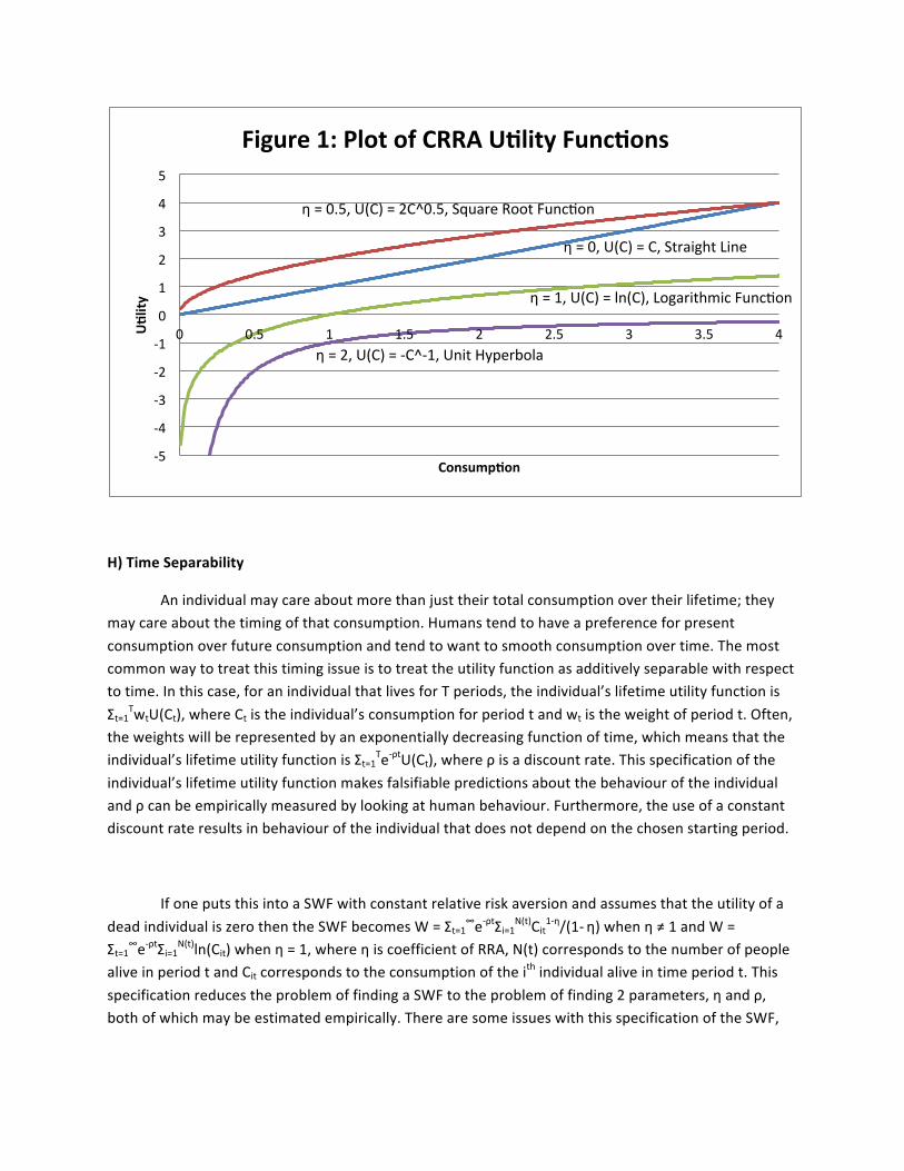
H)  Time  Separability  

  An  individual  may  care  about  more  than  just  their  total  consumption  over  their  lifetime;  they  may  care  about  the  timing  of  that  consumption.  Humans  tend  to  have  a  preference  for  present  consumption  over  future  consumption  and  tend  to  want  to  smooth  consumption  over  time.  The  most  common  way  to  treat  this  timing  issue  is  to  treat  the  utility  function  as  additively  separable  with  respect  to  time.  In  this  case,  for  an  individual  that  lives  for  T  periods,  the  individual’s  lifetime  utility  function  is  Σt=1TwtU(Ct),  where  Ct  is  the  individual’s  consumption  for  period  t  and  wt  is  the  weight  of  period  t.  Often,  the  weights  will  be  represented  by  an  exponentially  decreasing  function  of  time,  which  means  that  the  individual’s  lifetime  utility  function  is  Σt=1Te-­‐ρtU(Ct),  where  ρ  is  a  discount  rate.  This  specification  of  the  individual’s  lifetime  utility  function  makes  falsifiable  predictions  about  the  behaviour  of  the  individual  and  ρ  can  be  empirically  measured  by  looking  at  human  behaviour.  Furthermore,  the  use  of  a  constant  discount  rate  results  in  behaviour  of  the  individual  that  does  not  depend  on  the  chosen  starting  period.  

   

If  one  puts  this  into  a  SWF  with  constant  relative  risk  aversion  and  assumes  that  the  utility  of  a  dead  individual  is  zero  then  the  SWF  becomes  W  =  Σt=1∞e-­‐ρtΣi=1N(t)Cit

1-­‐η/(1-­‐  η)  when  η  ≠  1  and  W  =    Σt=1∞e-­‐ρtΣi=1N(t)ln(Cit)  when  η  =  1,  where  η  is  coefficient  of  RRA,  N(t)  corresponds  to  the  number  of  people  alive  in  period  t  and  Cit  corresponds  to  the  consumption  of  the  ith  individual  alive  in  time  period  t.  This  specification  reduces  the  problem  of  finding  a  SWF  to  the  problem  of  finding  2  parameters,  η  and  ρ,  both  of  which  may  be  estimated  empirically.  There  are  some  issues  with  this  specification  of  the  SWF,  

-­‐5  

-­‐4  

-­‐3  

-­‐2  

-­‐1  

0  

1  

2  

3  

4  

5  

0   0.5   1   1.5   2   2.5   3   3.5   4  UOlity

 

ConsumpOon  

Figure  1:  Plot  of  CRRA  UOlity  FuncOons  

η  =  0,  U(C)  =  C,  Straight  Line  

η  =  0.5,  U(C)  =  2C^0.5,  Square  Root  Funcyon  

η  =  1,  U(C)  =  ln(C),  Logarithmic  Funcyon  

η  =  2,  U(C)  =  -­‐C^-­‐1,  Unit  Hyperbola  

which  will  be  discussed  in  section  4.  However,  for  now  this  post  will  assume  that  this  specification  of  the  SWF  is  reasonable.  

 

I)  Expected  Social  Welfare  

  Since  maximizing  expected  utility  is  how  individuals  in  society  make  decisions  under  uncertainty  (for  EUT),  it  may  make  sense  that  maximizing  the  expected  value  of  the  SWF  (for  an  additively  separable  SWF)  is  how  society  should  make  decisions  under  uncertainty,  as  this  is  the  natural  extension  of  expected  utility  maximization  to  the  SWF.  However,  before  accepting  expected  social  welfare  maximization  as  a  reasonable  method  for  decision  making,  it  may  make  sense  to  look  at  some  other  common  decision  rules.  

   

  One  common  decision  rule  is  traditional  cost-­‐benefit  analysis.  Under  traditional  cost-­‐benefit  analysis,  one  tries  to  choose  the  policy  option  that  maximizes  the  net  present  value  of  benefits  minus  the  net  present  value  of  costs  (using  a  suitable  discount  rate).  The  theoretical  justification  for  cost-­‐benefit  analysis  is  that  if  the  there  is  little  uncertainty  about  the  future  and  any  policy  under  consideration  will  have  relatively  small  impacts  on  the  consumption  of  individuals  in  society  then  traditional  cost-­‐benefit  analysis  will  be  approximately  the  same  thing  as  expected  social  welfare  maximization.  However,  in  the  case  of  climate  change,  the  uncertainty  is  large  and  the  impact  of  policies  on  consumption  may  be  large,  so  traditional  cost-­‐benefit  analysis  is  inadequate.  However,  if  the  coefficient  of  RRA  is  zero  then  traditional  cost-­‐benefit  analysis  will  still  result  in  expected  social  welfare  maximization.  

 

  The  strong  precautionary  principle  is  a  decision  rule  that  I  frequently  see  argued  for  in  the  context  of  climate  change.  Under  the  strong  precautionary  principle,  if  there  is  any  risk  that  a  policy  may  have  a  negative  impact  on  society,  then  that  policy  should  not  be  taken.  There  are  numerous  problems  with  the  strong  precautionary  principle.  For  one,  the  strong  precautionary  principle  contradicts  itself.  For  example,  if  one  uses  the  strong  precautionary  principle  to  decide  whether  or  not  a  new  drug  should  be  allowed  on  the  market,  one  runs  the  risk  of  disallowing  many  perfectly  good  drugs,  causing  harm  to  society.  Thus  the  strong  precautionary  principle  has  a  risk  of  causing  harm  to  society  so  should  not  be  allowed  under  the  strong  precautionary  principle.  Secondly,  the  strong  precautionary  principle  has  many  bizarre  policy  implications.  For  example,  as  one  cannot  exclude  the  possibility  that  a  giant  flying  spaghetti  monster  may  appear  and  try  to  destroy  New  York.  Therefore,  under  the  strong  precautionary  principle,  the  US  government  should  spend  economic  resources  to  ensure  that  it  can  fend  off  any  attack  by  a  giant  flying  spaghetti  monster.  The  strong  precautionary  principle  also  suggests  that  society  should  ensure  that  all  cows  wear  snowshoes  (https://www.youtube.com/watch?v=6R999ZLlSdI).  Given  these  issues,  the  strong  precautionary  principle  does  not  seem  like  a  reasonable  method  to  make  decisions.  

Although,  if  the  coefficient  of  RRA  is  infinite  then  expected  social  welfare  maximization  reduces  to  the  strong  precautionary  principle.  

 

One  could  come  up  with  a  decision  rule  where  one  performs  a  traditional  cost-­‐benefit  analysis  but  uses  the  worst  case  scenario  of  a  non-­‐100%  confidence  interval  over  the  probability  distribution  of  different  outcomes.  This  would  allow  for  a  ranking  of  policy  responses  and  would  be  risk  averse  (yet  not  as  extreme  as  the  strong  precautionary  principle).  However,  such  a  decision  rule  would  not  be  very  desirable  since  the  choice  of  the  size  of  the  confidence  interval  would  be  arbitrary  and  it  does  not  have  the  property  where  if  the  probability  distribution  of  ECS  changes  to  suggest  a  higher  ECS  then  the  optimal  policy  response  may  not  necessarily  change  (see  Figure  2).  Furthermore,  such  a  decision  making  mechanism  would  not  have  a  strong  theoretical  justification,  unlike  expected  social  welfare  maximization.  The  rest  of  this  post  will  assume  that  expected  social  welfare  maximization  is  a  reasonable  way  to  make  policy  decisions  under  uncertainty.  

 

 

 

2.  Empirical  Estimates  of  the  Coefficient  of  Relative  Risk  Aversion:  

A)  Overview  of  Empirical  Evidence  

  It  may  be  helpful  to  look  at  empirical  evidence,  to  see  what  values  of  η,  the  coefficient  of  relative  risk  aversion  (also  sometimes  called  the  elasticity  of  marginal  utility  of  consumption),  may  be  reasonable.  The  literature  on  empirical  estimates  of  η  is  vast  and  there  are  many  different  methods  by  which  one  can  estimate  it,  from  looking  at  insurance  market  behaviour,  to  looking  at  market  price  elasticities,  to  setting  up  experiments.  Some  methods  are  more  reliable  than  others,  for  example,  for  

questionnaire  studies,  there  may  be  incentives  for  people  to  lie,  where  as  looking  at  how  individuals  manage  their  finances  may  give  a  more  accurate  picture  of  human  preferences.  If  you  wish  to  read  a  more  extensive  review  of  the  literature  of  measures  of  η,  then  I  suggest  a  literature  by  Outreville  (2014).  However,  this  post  will  just  cover  5  different  estimates,  in  order  to  keep  things  short  and  as  I  feel  that  these  5  are  the  most  relevant.  

 

B)  Tax  Structures  

  One  of  the  more  popular  ways  of  estimating  η,  at  least  when  it  comes  to  justifying  a  value  of  η  to  be  used  in  integrated  assessment  models,  is  to  look  at  the  tax  structure  of  society  to  get  an  idea  of  how  much  society  values  the  additional  dollar  of  a  poor  person  relative  to  the  additional  dollar  of  a  rich  person.  One  of  the  most  common  methods  by  which  one  can  do  this  is  a  method  first  suggested  by  Stern  (1977),  which  assumes  that  tax  distributions  roughly  follow  an  equal  sacrifice  principle  (i.e.  the  loss  of  utility  of  taxation  is  the  same  for  all  individuals  in  society).  Under  the  principle,  η  is  roughly  equal  to  ln(1-­‐tm)/ln(1-­‐ta),  where  tm  is  the  marginal  tax  of  the  individual  (i.e.  the  tax  they  would  have  to  pay  on  an  addition  dollar  of  income)  and  ta  is  the  average  tax  of  the  individual  (i.e.  total  tax  paid  divided  by  total  income).  One  of  the  more  recent  and  thorough  studies  that  uses  this  method  to  estimate  η  is  one  by  Evans  (2005).  In  this  study,  Evans  used  tax  structures  of  20  OECD  countries  and  obtained  a  best  estimate  of  η  of  1.41.  

 

  There  are  a  few  issues  with  using  this  method  to  estimate  η.  For  one,  a  tax  system  that  maximizes  the  social  welfare  of  society  is  unlikely  to  follow  the  equal  sacrifice  principle;  rather  an  optimal  tax  system  would  consist  roughly  of  a  combination  of  a  flat  tax  and  a  basic  income  (Mankiw  et  al.  2009),  which  would  result  in  the  poorest  in  society  having  an  negative  effective  tax  rate.  Secondly,  such  a  method  necessarily  constrains  η  to  be  greater  than  or  equal  to  1  for  progressive  tax  structures  and  cannot  deal  with  cases  where  the  effective  marginal  tax  rate  exceeds  100%  (this  can  occur  if  there  is  a  strong  welfare  trap).  Thirdly,  governments  with  very  similar  populations  are  observed  to  have  very  different  taxation  policy  (example:  compare  North  Korea  with  South  Korea,  or  compare  consumption  taxes  in  the  USA  compared  to  Western  Europe),  which  suggests  that  governments  are  very  bad  at  evaluating  optimal  taxation  policy.  

 

  Lastly,  the  optimal  tax  structure  depends  on  more  than  just  η.  Optimal  tax  structures  depend  greatly  on  how  much  people  value  their  leisure  time  and  therefore  the  effect  that  tax  structures  will  have  on  the  incentive  for  individuals  to  work.  The  uncertainty  of  the  effect  of  taxation  on  the  willingness  of  people  to  work  is  fairly  large  (estimates  of  the  labour  supply  elasticity  of  taxation  tend  to  vary  from  0.1  to  0.7).  Even  for  the  same  value  of  η  (say  η  =  1),  a  low  labour  supply  elasticity  may  suggest  a  very  libertarian  optimal  tax  structure,  where  as  a  high  labour  supply  elasticity  may  suggest  a  very  socialist  optimal  tax  structure.  As  people  generally  value  their  leisure  time,  and  more  progressive  tax  structures  

generally  result  in  people  having  more  leisure  time  (as  they  have  less  employment),  estimates  using  this  method  will  tend  to  overestimate  η,  as  they  ignore  the  fact  that  people  value  their  leisure  time.  In  addition,  optimal  taxation  also  depends  on  the  level  of  income  inequality  in  society  (Mankiw  et  al.  2009);  a  higher  level  of  income  inequality  suggests  that  a  social  welfare  maximizing  tax  system  becomes  more  income  redistributing.  Overall,  while  looking  at  tax  structures  can  give  useful  insight  into  the  value  of  η,  such  an  approach  has  numerous  flaws.  

 

C)  Labour  Market  Behaviour  

Another  interesting  way  to  estimate  η  is  to  look  at  labour  market  behaviour.  One  of  the  best  studies  that  takes  this  approach  is  a  paper  by  Chetty  (2006).  In  this  paper,  Chetty  invents  a  method  to  estimate  η  by  taking  advantage  of  uncertainty  in  future  labour  market  conditions  and  using  data  on  labour  market  behaviour.  Chetty’s  best  estimate  of  η  is  0.97,  which  suggests  that  utility  is  roughly  a  logarithmic  function  of  consumption.  However,  this  estimate  assumes  that  the  complementariness  of  leisure  and  consumption  is  0.15.  The  uncertainty  of  this  complementariness  suggests  that  this  estimate  may  be  an  underestimate  (perhaps  by  as  much  as  33%).  However,  even  after  taking  this  uncertainty  into  account,  Chetty  finds  that  a  value  of  η  greater  than  2  is  simply  inconsistent  with  labour  market  behaviour.  Thus  Chetty’s  paper  provides  a  good  upper  bound  for  η.  

 

D)  Happiness  Surveys  

  Arguably,  one  of  the  best  estimates  for  η  has  been  performed  by  Layard  et  al.  (2008).  The  approach  by  Layard  et  al.  takes  advantage  of  the  fact  that  happiness  is  correlated  with  utility  and  uses  data  on  self  reported  happiness  from  over  200,000  individuals  to  estimate  η.  Initially,  Layard  et  al.  assume  that  happiness  is  roughly  a  linear  function  of  utility  to  estimate  η  as  1.26  (with  95%  confidence  interval  of  [1.15,1.37]).  However,  happiness  is  not  necessarily  a  linear  function  of  utility,  more  generally  it  can  be  any  positive  monotonic  transformation  of  utility.  To  check  for  this  possibility,  Layard  et  al.  relax  their  linearity  consumption  slightly  to  find  a  better  estimate  of  1.24  (with  95%  confidence  interval  of  [1.14,1.35]).  In  both  cases,  Layard  et  al.  control  for  various  other  explanatory  factors  for  differences  in  self  reported  happiness  such  as  leisure  time.  Thus  the  Layard  et  al.  result  doesn’t  have  a  bias  due  to  not  adequately  taking  into  account  leisure  time,  unlike  the  results  of  Evans  and  Chetty.  

 

  It  may  seem  like  unlikely  coincidence  for  self-­‐reported  happiness  to  be  a  roughly  linear  function  of  utility.  However,  if  humans  follow  the  behaviour  of  EUT,  then  humans  may  have  a  natural  tendency  to  treat  happiness  as  a  linear  function  of  utility  because  then  the  expected  happiness  maximization  will  result  in  expected  utility  maximization.  One  issue  with  using  happiness  surveys  is  that  happiness  and  utility  may  become  uncorrelated  in  cases  of  misinformation  (the  saying  ‘ignorance  is  bliss’  comes  to  

mind),  so  one  should  be  a  bit  skeptical  about  the  results.  Overall,  the  Layard  et  al.  result  using  happiness  survey  data  gives  a  surprisingly  robust  and  surprisingly  well  constrained  estimate  of  η.  

 

E)  Ramsey  Equation  

  If  the  individuals  in  society  have  a  lifetime  utility  function  of  Σt=1Te-­‐ρt  Cit1-­‐η/(1-­‐  η)  when  η  ≠  1  and  

Σt=1Te-­‐ρtln(Ct)  when  η  =  1,  where  T  is  the  lifetime  of  the  individual,  and  ρ  is  the  discount  rate,  then  this  has  predictions  about  the  interest  rate  of  society.  In  such  a  society,  r  =  ρ  +  ηg,  where  r  is  the  real  riskless  after-­‐tax  interest  rate,  ρ  is  known  as  the  social  rate  of  time  preference,  η  is  the  coefficient  of  RRA,  and  g  is  the  growth  rate  of  real  purchasing  price  parity  GDP  per  capita  (see  Creedy  and  Guest  2008  for  a  derivation).  This  equation  is  known  as  the  Ramsey  equation.  

 

  Using  the  Ramsey  equation,  it  is  possible  to  estimate  both  ρ  and  η  by  using  data  on  real  interest  rates  and  rates  of  real  GDP  per  capita  growth.  However,  in  the  short  run  it  is  possible  for  a  country’s  interest  rates  to  diverge  from  what  is  expected  by  the  Ramsey  equation  and  actually  this  may  be  expected  based  on  the  policies  of  most  central  banks  in  the  word  (which  tend  to  roughly  follow  a  rule  known  as  the  Taylor  rule).  However,  in  the  long  run,  Ramsey’s  equation  should  be  roughly  satisfied,  so  one  may  be  able  to  estimate  η  by  comparing  real  interest  rates  and  real  GDP  per  capita  growth  rates  averaged  over  a  long  period  of  time  between  countries.  Anthoff  et  al.  (2009)  use  data  from  27  OECD  countries  over  a  36  year  period  and  obtain  a  best  estimate  of  η  of  1.18.  This  is  similar  to  the  estimate  of  Layard  et  al.  although  the  uncertainty  of  the  Anthoff  et  al.  estimate  is  much  higher.  One  issue  with  this  estimate  is  that  the  social  rate  of  time  preference  ρ  may  be  different  for  different  countries.  In  particular,  countries  with  higher  life  expectancies  may  be  expected  to  have  lower  values  of  ρ.  Since  life  expectancy  is  positively  correlated  with  real  GDP  per  capita,  and  real  GDP  per  capita  is  negatively  correlated  with  real  GDP  per  capita  growth  over  the  period  of  time  used  by  Anthoff  et  al.,  such  a  specification  error  may  suggest  that  this  estimate  by  Anthoff  et  al.  is  an  overestimate.  

   

  If  people  do  not  value  the  future  more  than  the  present,  then  ρ  cannot  be  less  than  zero.  As  a  result,  η  <  r/g  provides  an  upper  bound  on  the  value  of  η.  According  to  the  World  Bank,  the  average  real  riskless  interest  rate  of  the  USA  from  1995-­‐2014  was  3.88%.  In  addition,  the  tax  on  capital  gains  in  the  USA  is  approximately  19.1%  (http://taxfoundation.org/article/capital-­‐gains-­‐rate-­‐country-­‐2011-­‐oecd).  This  suggests  that  the  after-­‐tax  average  real  riskless  interest  rate  for  this  period  was  3.14%.  By  comparison,  the  average  rate  of  real  GDP  per  capita  growth  for  the  USA  over  this  period  was  1.475%.  This  suggests  that  η  greater  than  2.14  would  be  inconsistent  with  empirical  evidence.  This  agrees  with  the  result  by  Chetty,  that  η  greater  than  2  is  inconsistent  with  empirical  observations.  

 

F)  Statistical  Value  of  Life  

  How  people  make  decisions  when  it  comes  to  the  probability  of  death  can  also  be  used  to  estimate  η.  If  the  average  individual  in  society  is  indifferent  about  taking  a  risk  that  has  a  (1  –  α)  chance  of  increasing  their  consumption  by  ΔC  and  an  α  chance  of  killing  them,  where  α  and  ΔC/C  are  both  very  small,  then  ΔC/α  is  known  as  the  statistical  value  of  life  (SVL).  If  the  utility  of  death  corresponds  to  a  consumption  level  of  zero  then  this  suggests  that  U(C)  =  (1  –  α)U(C  +  ΔC)  =>  C1-­‐η/(1  -­‐  η)  =  (1  –  α)(C  +  ΔC)1-­‐η/(1  -­‐  η)  =>  C1-­‐η  =  (1  –  α)C1-­‐η(1  +  ΔC/C)1-­‐η  ≈  (1  –  α)C1-­‐η(1  +  (1  -­‐  η)ΔC/C)  =>  1  ≈  1  –  α  +  (1  -­‐  η)ΔC/C  =>  η  =  1  –  αC/ΔC  =  1  –  C/SVL  

 

  For  the  USA,  the  SVL  is  approximately  200  times  annual  per  capita  income  (Cline  1992).  Furthermore,  the  life  expectancy  for  the  USA  in  1992  was  72  years.  If  the  average  person  is  middle  aged,  then  this  suggests  that  they  would  have  on  average  36  years  of  remaining  life.  This  means  that  total  remaining  consumption  for  the  individual  would  be  roughly  36  times  annual  per  capita  income.  Putting  this  information  into  the  above  equation  gives  η  =  0.82.  Of  course  this  is  a  very  rough  estimate  with  numerous  problems,  but  it  does  illustrate  how  statistical  value  of  life  estimates  can  be  used  to  estimate  η.  Note  that  a  finite  statistical  value  of  life  implies  that  η  <  1.  

 

 

3.  Other  Considerations  of  CRRA  Utility  Functions  

A)  Finite  Statistical  Value  of  Life?  

  The  equation  derived  in  2F  suggests  that  if  η  ≥  1  then  the  statistical  value  of  life  for  a  CRRA  utility  function  cannot  be  finite.  Yet  empirical  estimates  suggest  that  the  SVL  is  finite  and  in  everyday  society  it  is  observed  that  people  frequently  do  risky  activities  that  put  their  lives  at  risk,  from  smoking,  to  talking  on  a  cellphone  while  driving,  to  sky  diving.  To  show  the  absurdity  of  an  infinite  SVL,  take  the  simple  activity  of  eating  a  potato  chip.  Potato  chips  are  unhealthy  and  can  increase  your  chance  of  dying  from  heart  disease.  Even  if  the  increase  in  the  probability  of  dying  from  eating  a  potato  chip  is  very  small  (say  one  in  one  sextillion)  it  is  still  finite,  and  the  pleasure  gained  from  eating  a  potato  chip  is  finite,  thus  an  expected  utility  maximizing  individual  would  never  eat  that  potato  chip  if  they  assigned  an  infinite  value  to  their  own  life.  Given  that  people  eat  potato  chips  in  society,  the  SVL  is  likely  finite.  

 

  Is  possible  to  have  η  ≥  1  and  a  finite  SVL?  It  is  possible  provided  that  the  constantness  of  the  coefficient  of  RRA  breaks  down  at  low  levels  of  consumption  and  that  the  limit  of  η  as  consumption  approaches  zero  is  less  than  1.  Why  might  η  be  less  than  1  for  very  low  levels  of  consumption?  Well  one  reason  is  that  people  become  increasingly  desperate  in  extreme  poverty  and  in  extreme  poverty  the  individual’s  remaining  life  expectancy  is  strongly  dependant  on  their  level  of  consumption.  A  person  that  is  starving  to  death  may  only  have  a  month  or  two  of  remaining  life;  however,  if  they  take  a  risk  they  may  be  able  to  afford  enough  food  to  not  starve  to  death,  which  may  give  them  many  years  of  

additional  life.  In  such  a  scenario,  individuals  may  actually  become  risk  loving  (η  <  0),  which  means  that  the  Pigou-­‐Dalton  principle  may  be  violated  for  individuals  that  are  starving  to  death.  One  way  to  illustrate  violation  of  the  Pigou-­‐Dalton  principle  is  to  consider  two  individuals  stranded  on  a  boat  in  the  Pacific  Ocean.  In  this  scenario,  if  the  two  individuals  do  nothing  both  will  starve  to  death  before  receiving  help,  but  if  one  individual  eats  the  other  individual  then  the  remaining  individual  will  live  long  enough  to  receive  help  and  live  on  for  many  years.  In  this  case,  social  welfare  maximization  suggests  that  one  individual  should  cannibalize  the  other  individual;  thus  increased  consumption  inequality  is  desirable,  which  suggests  that  the  Pigou-­‐Dalton  principle  is  violated.  

 

  The  previous  paragraph  suggests  that  one  may  be  able  to  observe  a  constant  η  ≥  1  for  most  consumption  levels  and  a  finite  statistical  life  provided  that  the  constantness  of  η  breaks  down  in  cases  of  extreme  poverty.  In  particular,  if  the  reason  for  this  break  down  is  due  to  starvation  and  the  effect  of  low  levels  of  consumption  on  remaining  life  expectancy  then  there  should  be  a  discontinuity  in  human  behaviour  around  the  subsistence  level  of  real  GDP  per  capita.  Caballero  (2010)  has  found  empirical  evidence  consistent  with  this  hypothesis.  Caballero  performed  experiments  with  impoverished  Colombians  to  try  to  determine  their  behaviour  under  risk.  In  the  study,  Caballero  uses  a  subsistence  level  of  real  GDP  per  capita  of  148,000  2009  Colombian  Pesos  per  month  (this  corresponds  to  about  $1445  2009  USD  per  year  in  purchasing  price  parity)  to  try  to  see  if  there  is  a  discontinuity  in  risk  aversion  around  the  subsistence  level.  Caballero  finds  that  individuals  just  above  the  subsistence  level  of  real  GDP  per  capita  are  far  more  risk  averse  than  people  just  below  the  subsistence  level  of  real  GDP  per  capita.  

 

  Given  that  the  vast  majority  of  the  world  has  a  level  of  income  above  the  subsistence  level  of  real  GDP  per  capita,  and  that  this  should  continue  over  the  next  hundred  years,  the  usage  of  Σt=1Te-­‐ρt  Cit

1-­‐η/(1-­‐  η)  when  η  ≠  1  and  Σt=1Te-­‐ρtln(Ct)  when  η  =  1  as  the  SWF  may  be  reasonable  even  if  η  is  a  constant  that  is  greater  than  or  equal  to  1  for  the  application  of  determining  optimal  policy  with  respect  to  climate  change.  However,  one  should  note  that  such  a  CRRA  utility  function  would  break  down  for  dead  people  and  for  people  in  extreme  poverty.  A  better  utility  function  to  be  used  for  expected  social  welfare  maximization  might  be  a  piecewise  continuous  function  that  is  a  CRRA  utility  function  above  the  subsistence  level  of  consumption  and  something  else  (such  as  a  polynomial)  below  the  subsistence  level.  Lastly,  I  want  to  point  out  that  this  discontinuity  in  behaviour  around  the  subsistence  level  may  explain  the  behaviour  of  loss  aversion  in  humans.  For  most  of  human  history,  humans  lived  at  roughly  the  subsistence  level  of  consumption,  where  the  behaviour  of  loss  aversion  is  consistent  with  expected  utility  maximization.  Thus  there  would  have  been  no  selectional  pressure  against  individuals  with  loss  aversion  behaviour  (and  it  may  have  been  an  evolutionary  advantage  as  it  may  have  allowed  for  decisions  to  be  made  with  less  cognitive  resources).  

 

B)  St.  Petersburg  Paradox  

  A  famous  problem  that  is  relevant  to  the  discussion  of  human  preferences  is  known  as  the  St.  Petersburg  paradox  (see  https://en.wikipedia.org/wiki/St._Petersburg_paradox).  In  the  St.  Petersburg  paradox,  an  individual  is  offered  to  pay  the  following  fee  of  $x  and  play  the  following  game:  the  individual  has  a  1/2  chance  of  winning  $2,  a  1/4  chance  of  winning  $4,  a  1/8  chance  of  winning  $8  and  so  on.  Most  individuals  are  only  willing  to  pay  a  finite  fee  to  play  the  game,  yet  the  expected  winnings  of  the  game  is  infinite.  How  can  this  be?  The  original  St.  Petersburg  paradox  was  resolved  using  EUT.  

 

However,  Menger  (1934)  showed  that  games  similar  to  the  St.  Petersburg  paradox  suggest  that  the  utility  of  infinite  consumption  is  necessarily  finite.  This  suggests  that  η  must  be  greater  than  1  as  consumption  approaches  infinity.  Nobel  prize  winner  Kenneth  Arrow  argued  in  the  60’s  that  the  result  by  Menger  combined  with  finite  statistical  value  of  life  suggest  that  the  η  in  humans  cannot  vary  much  from  1,  thus  utility  is  an  approximately  logarithmic  function  of  consumption.  Overall,  finite  statistical  life,  the  results  by  Caballero  and  the  result  by  Menger  suggest  that  η  is  not  a  constant  function  of  income.  Below  is  a  sketch  of  one  possibility  of  how  η  may  vary  with  level  of  consumption  in  order  to  be  consistent  with  these  observations.  

 

 

C)  Interesting  Things  about  Logarithmic  Utility  

  There  are  a  few  interesting  things  about  η  =  1  that  are  worth  mentioning.  Firstly,  η  =  1  is  arguably  expected  under  utility  theory  as  argued  by  Sinn  (2003)  and  Zhang  et  al.  (2014),  so  there  might  be  an  evolutionary  basis  for  η  ≈  1.  Secondly  a  logarithmic  utility  function  maximizes  the  long  run  size  of  an  individual’s  stock  portfolio,  so  individuals  with  η  =  1  preferences  may  be  the  most  successful  in  society.  Finally,  the  usage  of  η  =  1  significantly  simplifies  calculating  the  SWF.  Consumption  is  roughly  proportional  to  economic  output  (assuming  constant  savings  rate)  and  real  GDP  per  capita  in  purchasing  price  parity  is  inversely  proportional  to  prices.  Thus  the  usage  of  η  =  1  means  that  the  maximization  of  

the  SWF  does  not  depend  strongly  on  the  savings  rate  nor  on  how  purchasing  price  parity  is  determined  and  one  can  replace  consumption  in  the  social  welfare  function  with  an  individual’s  real  GDP.    

 

In  addition,  the  production  function  is  usually  specified  as  a  Cobb-­‐Douglas  production  function,  where  different  factors  of  production  are  multiplicatively  separable  (Nordhaus’  DICE  integrated  assessment  model  uses  such  a  production  function  where  the  economic  impact  of  climate  change  as  well  as  the  costs  of  mitigation  are  multiplicatively  separable).  As  a  result,  the  logarithm  of  a  Cobb-­‐Douglas  production  function  is  additively  separable,  which  means  that,  after  one  takes  the  derivatives  of  the  SWF,  many  of  the  terms  go  to  zero.  The  maximization  of  such  a  social  welfare  function  will  not  depend  strongly  on  things  like  the  growth  rate  of  productivity  or  the  level  of  education  of  individuals  in  society,  so  the  decision  making  will  be  more  robust.  Lastly,  Cobb-­‐Douglas  functions  are  generally  relatively  easy  to  estimate  (due  to  the  fact  that  the  logarithm  is  additively  separable,  so  one  can  estimate  such  a  function  with  a  simple  linear  regression),  so  there  is  far  more  literature  on  empirical  estimates  of  the  economic  impacts  of  climate  change  and  mitigation  using  Cobb-­‐Douglas  production  functions  than  other  functional  forms.  One  can  use  the  variation  in  economic  output  across  the  globe  to  estimate  economic  impacts  of  climate  change  and  mitigation  costs  (examples  include  Nordhaus  et  al.  2006,  Zhao  2011  and  Burke  et  al.  2015);  such  a  method  has  the  added  benefit  of  avoiding  publication  bias  in  the  literature.  

 

D)  Coefficients  of  Relative  Risk  Aversion  Used  Elsewhere    

To  end  this  section,  I  will  discuss  the  values  of  η  that  have  been  used  by  other  people.  Stern  (2007)  used  a  value  of  1  in  his  famous  Stern  Review.  Nordhaus  (Nordhaus  and  Sztorc  2013)  currently  uses  a  value  of  1.45  as  the  default  parameter  in  his  DICE  integrated  assessment  model,  although  he  used  a  value  of  2  in  the  past.  Tol  (Anthoff  et  al.  2009)  currently  uses  a  value  of  1.47  in  his  FUND  integrated  assessment  model.  The  United  Kingdom  Treasury  currently  uses  a  value  of  1,  which  was  reduced  from  1.5  a  few  years  ago.  By  comparison  the  5  values  that  I  discussed  in  section  2  were  1.41  (Evans  2005  using  tax  structures  of  20  OECD  countries),  0.97  (Chetty  2006  using  labour  market  behaviour),  1.24  (Layard  et  al.  2008  using  happiness  surveys),  1.18  (Anthoff  et  al.  2009  using  Ramsey’s  equation  and  data  from  27  OECD  countries)  and  0.82  (this  post  using  statistical  value  of  life  from  Cline  1992).  Given  the  range  of  estimates,  a  value  of  η  outside  of  the  range  [0.5,2.0]  is  inconsistent  with  empirical  observations  (the  upperbound  was  argued  by  Chetty,  and  the  lowerbound  is  partially  subjective,  although  is  probably  a  bit  generous  given  the  range  of  estimates  in  Outreville  2014).  This  suggests  that  utility  as  a  function  of  consumption  is  somewhere  between  a  square  root  function  and  a  unit  hyperbola.  

 

 

4.  Choice  of  Discount  Rate:  

A)  Values  Used  for  Cost-­‐Benefit  Analysis  

  In  addition  to  determining  a  reasonable  value  of  the  coefficient  of  relative  risk  aversion  η,  a  reasonable  value  of  the  discount  rate  ρ  needs  to  be  determined  in  order  to  have  a  well  justified  social  welfare  function.  It  may  help  to  examine  what  discount  rates  are  currently  used  in  cost-­‐benefit  analyses  in  order  to  determine  a  reasonable  value  of  ρ.  The  Office  of  Management  and  Budget  (OMB)  recommends  a  default  rate  of  7%  for  base-­‐case  analysis  (https://www.whitehouse.gov/omb/circulars_a094/).  Some  have  suggested  that  because  of  this,  a  7%  discount  rate  should  be  applied  in  the  context  of  making  decisions  about  climate  change.  However,  there  are  a  few  issues  with  using  this  discount  rate  for  expected  social  welfare  maximization.  The  justification  for  this  rate,  according  to  the  OMB,  is  “This  rate  approximates  the  marginal  pretax  rate  of  return  on  an  average  investment  in  the  private  sector  in  recent  years.”  Yet  this  was  written  in  1992,  so  is  23  years  out  of  date.  Figure  4  shows  how  market  interest  rates  have  evolved  over  the  past  few  decades  for  the  USA  according  to  the  World  Bank.  

 

 

From  Figure  4,  it  is  clear  that  interest  rates  peaked  in  the  80’s  and  have  slowly  declined  since.  The  interest  rates  during  the  few  years  prior  to  1992  were  higher  than  the  interest  rates  in  recent  years.  Therefore,  the  7%  rate  seems  inappropriate  for  today  and  perhaps  the  rate  by  the  OMB  should  be  updated  to  be  more  reflective  of  interest  rates  in  recent  years  (perhaps  4%  would  be  more  appropriate).  As  a  comparison,  the  recommended  rates  in  other  countries  are  8%  (Canada,  Australia,  New  Zealand  and  China),  5%  (Italy),  4%  (France),  3.5%  (UK)  and  3%  (Germany).  

 

-­‐2.00  

0.00  

2.00  

4.00  

6.00  

8.00  

10.00  

1960   1970   1980   1990   2000   2010   2020  

Real  In

terest  Rate  (%

)  

Year  

Figure  4:  Real  Interest  Rates  vs  Time  for  USA  

  Secondly,  there  is  the  question  of  whether  or  not  to  use  risk  free  interest  rates.  For  some  applications,  such  as  using  traditional  cost-­‐benefit  analysis  to  determine  whether  or  not  to  finance  a  new  bridge,  adding  a  risk  premium  to  the  discount  rate  may  make  sense  as  there  is  a  chance  that  one  may  not  be  able  to  get  a  return  from  that  investment  (the  bridge  might  get  destroyed  by  a  natural  disaster  or  a  war,  or  it  might  get  expropriated  by  the  government).  In  the  case  of  expected  social  welfare  maximization,  one  tries  to  take  into  account  the  probability  and  outcome  of  all  possibilities  including  unlikely  events,  so  such  an  approach  already  takes  risk  into  account.  The  discount  rate  used  in  the  SWF  for  social  welfare  maximization  reflects  the  trade-­‐off  in  consumption  between  periods  under  certainty,  so  risk  free  interest  rates  should  be  used.  

 

Thirdly,  the  discount  rate  in  the  SWF  reflects  how  much  individuals  value  the  utility  of  future  consumption  relative  to  the  value  of  present  consumption,  therefore  it  may  be  more  appropriate  to  look  at  how  much  consumers  in  the  market  are  valuing  future  consumption  relative  to  present  consumption.  The  return  that  a  consumer  gets  on  their  savings  depends  on  the  after-­‐tax  interest  rate,  not  the  pretax  interest  rate.  Therefore,  the  use  of  pretax  interest  rates  is  more  appropriate.  As  mentioned  earlier,  the  average  after-­‐tax  real  riskless  interest  rate  over  the  past  20  years  was  3.14%,  which  is  roughly  the  3%  discount  rate  recommended  by  the  OMB  for  decisions  that  primarily  affect  the  consumption  of  individuals  in  society.  

 

B)  Ramsey  Equation  

  The  after-­‐tax  real  riskless  interest  rate  represents  how  individuals  in  society  value  future  consumption  relative  to  present  consumption.  However,  that  isn’t  necessarily  the  same  thing  as  how  individuals  in  society  value  future  utility  of  consumption  relative  to  present  utility  of  consumption.  As  explained  in  2E,  if  a  society  consists  of  lifetime  utility  maximizing  individuals  with  utility  functions  Σt=1Te-­‐ρt  Cit

1-­‐η/(1-­‐  η)  when  η  ≠  1  and  Σt=1Te-­‐ρtln(Ct)  when  η  =  1,  then  r  =  ρ  +  ηg,  where  r  is  the  real  riskless  after-­‐tax  interest  rate,  ρ  is  the  social  rate  of  time  preference,  η  is  the  coefficient  of  RRA,  and  g  is  the  growth  rate  of  real  GDP  per  capita.  This  equation  is  known  as  the  Ramsey  equation.  Note  that  this  equation  suggests  that  real  interest  rates  depend  on  the  real  GDP  per  capita  growth  rate,  which  helps  to  explain  some  of  the  variation  in  observed  interest  rates  in  figure  4.  

 

  As  a  quick  example,  if  one  uses  r  =  3.14%  and  g  =  1.475%  (these  correspond  to  the  average  values  of  the  US  over  the  past  20  years)  and  η  =  1  (logarithmic  utility)  then  this  suggests  that  one  should  use  ρ  =  1.665%  in  order  to  be  consistent  with  the  Ramsey  equation.  More  generally,  if  η  is  in  the  interval  [0.5,2.0]  then  the  Ramsey  equation  suggests  that  ρ  is  in  the  interval  [0.2%,2.4%].  By  comparison,  Nordhaus  and  Sztorc  (2013)  use  η  =  1.45  and  ρ  =  1.5%  for  DICE  and  Anthoff  et  al.  (2009)  use  η  =  1.47  and  ρ  =  1.07%  for  FUND;  both  sets  of  values  are  roughly  consistent  with  Ramsey’s  equation.  One  possible  explanation  for  the  value  of  ρ  is  that  ρ  represents  the  probability  of  a  consumer  dying  in  a  given  year  

(and  therefore  be  unable  to  benefit  from  any  savings).  As  a  comparison,  the  average  global  life  expectancy  is  71  years  for  2013;  the  inverse  of  this  is  1.41%  per  year.  Note  that  even  though  the  Ramsey  equation  suggests  using  a  lower  discount  rate  than  what  is  suggested  for  traditional  cost-­‐benefit  analysis,  this  lower  discount  rate  is  offset  by  the  fact  that  η  takes  into  account  intergeneration  inequality  (future  generations  will  be  richer  than  present  ones).  

 

C)  Zero  Discount  Rate?  

  Some  individuals,  such  as  Stern  (2007),  have  taken  the  moral  position  that  discounting  with  ρ  >  0  is  immoral  because  it  values  present  generations  more  than  future  generations  and  therefore  values  people  unequally.  There  are  a  few  issues  with  such  a  position.  For  one,  with  ρ  =  0,  the  SWF  does  not  converge  and  therefore  cannot  generally  be  evaluated  (so  policy  decisions  cannot  be  made);  ρ  =  0  suggests  that  all  time  periods  have  no  weight  in  the  SWF,  except  the  limit  of  the  period  as  time  approaches  infinity  (which  has  all  the  weight,  but  cannot  be  reasonably  evaluated  as  our  universe  would  likely  be  long  dead  by  then).  Rather  than  being  moral,  ρ  =  0  is  arguably  immoral  as  it  would  suggest  that  the  present  has  no  value  (If  you  are  interested  in  a  strong  axiomatic  basis  for  using  a  positive  discount  rate,  I  recommend  Creedy  and  Guest  2008,  3.1).  Furthermore,  with  ρ  >  0,  the  SWF  can  be  numerically  approximated  by  only  evaluating  the  first  X  finite  periods,  provided  that  X  is  sufficiently  larger  than  the  inverse  of  ρ;  for  a  ρ  of  1.5%,  the  first  200-­‐300  years  are  likely  sufficient  for  expected  social  welfare  maximization.  

 

A  second  issue  with  the  ρ  =  0  position  is  that  it  has  very  strange  policy  implications  outside  of  the  context  of  climate  change.  For  example,  it  suggests  that  expected  social  welfare  maximizing  governments  should  save  more  money  for  future  generations  as  long  as  the  pretax  real  riskless  interest  rate  exceeds  ηg.  This  suggests  that  governments  around  the  world  should  run  very  large  surpluses  in  order  to  save  large  amounts  of  money  for  future  generations,  rather  than  run  deficits  as  they  are  now.  Unless  one  also  advocates  that  governments  should  run  very  large  surpluses  to  do  this,  then  suggests  that  ρ  should  be  zero  when  it  comes  to  making  decisions  about  climate  change  would  be  inconsistent.  

 

A  third  issue  with  the  ρ  =  0  position  is  feasibility.  Ultimately,  it  is  individuals  alive  today  that  are  currently  negotiating  to  come  to  an  agreement  in  Paris,  and  it  is  voters  alive  today  that  they  are  supposed  to  represent.  The  ρ  implied  by  the  Ramsey  equation  arguably  not  only  tells  us  how  much  individuals  value  their  future  consumption  but  also  how  much  individuals  value  future  generations.  If  current  generations  valued  future  generations  as  much  as  themselves  then  current  generations  would  likely  increase  savings  for  future  generations  (such  as  for  their  children  and  grandchildren)  until  r  =  ηg.  So  if  market  interest  rates  suggest  that  ρ  >  0,  then  this  suggests  that  current  generations  likely  value  future  generations  less  than  current  generations.  If  a  policy  can  only  be  justified  by  valuing  future  

generations  more  than  current  generations  value  those  future  generations,  then  current  generations  will  have  no  incentive  to  go  with  that  policy.  Thus,  such  a  policy  is  not  feasible.  

 

Despite  the  issues  with  the  ρ  =  0  position,  it  does  bring  up  the  problem  that  how  much  individuals  discount  their  own  future  utility  might  not  be  the  same  as  how  much  individuals  discount  future  generations.  More  generally,  the  SWF  could  be  written  as  W  =  Σt=1∞e-­‐ζtΣi=1M(t)  Σs=tt-­‐1+T(i,t)e-­‐ρ(s-­‐t)Cist

1-­‐

η/(1-­‐  η)  when  η  ≠  1  and  W  =  Σt=1∞e-­‐ζtΣi=1M(t)  Σs=tt-­‐1+T(i,t)e-­‐ρ(s-­‐t)ln(Cist)  when  η  =  1,  where  ζ  is  the  rate  at  which  future  generations  are  discounted,  ρ  is  the  rate  at  which  individuals  discount  their  own  utility,  M(t)  is  the  number  of  individuals  born  at  time  t,  T(i,t)  is  the  life  expectancy  of  the  ith  individual  born  at  time  t,  and  Cist  is  the  consumption  of  the  ith  individual  born  at  time  t  in  period  s.  The  above  specification  allows  for  ζ  and  ρ  to  differ,  but  is  otherwise  essentially  the  same  SWF.  Fortunately,  it  might  be  possible  to  estimate  ζ  from  empirical  evidence  (such  as  by  looking  at  how  much  inheritance  people  leave  to  their  offspring  or  by  looking  at  happiness  surveys).  Unfortunately,  as  far  as  I  can  tell,  there  is  basically  zero  literature  on  estimating  ζ.  Due  to  lack  of  estimates,  it  may  make  sense  to  appeal  to  Occam’s  razor  and  assume  that  ζ  =  ρ  until  empirical  evidence  suggests  otherwise.  

 

D)  Non-­‐Constant  Discount  Rate?  

  So  far,  the  assumption  has  been  that  the  discount  rate  is  constant.  However,  the  discount  rate  does  not  necessarily  have  to  be  constant.  Some  have  argued  that  a  declining  discount  rate  over  time  may  make  sense.  For  example,  Arrow  et  al.  (2012  and  2014),  suggest  that  uncertainty  about  the  future,  particularly  uncertainty  of  the  growth  rate  of  consumption,  can  cause  a  declining  certainty-­‐equivalent  discount  rate.  Thus  it  may  make  sense  to  use  a  declining  discount  rate  if  one  is  performing  traditional  cost-­‐benefit  analysis.  However,  in  the  case  of  expected  social  welfare  maximization,  uncertainty  about  the  future  is  already  taken  into  account  by  taking  into  account  the  entire  probability  distribution  of  outcomes.  Thus,  the  use  of  declining  certainty-­‐equivalent  discount  rates  for  expected  social  welfare  maximization  would  be  double  counting  and,  therefore,  would  not  make  sense.  

 

  Another  way  that  declining  discount  rates  can  be  justified  is  on  the  observation  that  life  expectancy  is  generally  increasing  over  time.  If  the  social  rate  of  time  preference  is  inversely  related  to  the  life  expectancy  of  humans,  then  it  may  make  sense  to  use  a  declining  social  rate  of  time  preference.  However,  the  magnitude  of  such  an  effect  over  the  next  century  is  likely  small  compared  to  the  magnitude  of  the  uncertainty  of  the  social  rate  of  time  preference.  Preference  for  simplicity  suggests  that  it  may  make  sense  to  use  a  constant  social  rate  of  time  preference  until  the  uncertainty  of  its  magnitude  is  reduced  and  there  is  a  better  justification  for  declining  social  rate  of  time  preference.  Also,  if  one  does  want  to  use  social  rates  of  time  preference  that  depend  on  life  expectancy  then  one  may  want  to  do  it  in  such  a  way  that  the  anonymity  principle  is  not  violated  (such  as  having  the  social  rate  of  time  preference  be  the  same  for  everyone  in  any  given  year).  

 

E)  Population  and  Life  Expectancy  Concerns  

  The  SWF  given  in  1H  was  W  =  Σt=1∞e-­‐ρtΣi=1N(t)Cit1-­‐η/(1-­‐  η)  when  η  ≠  1  and  W  =  Σt=1∞e-­‐ρtΣi=1N(t)ln(Cit)  

when  η  =  1.  Such  a  SWF  is  a  Benthamite  SWF  (named  after  18th  century  philosopher  Jeremy  Bentham).  Such  a  SWF  may  be  reasonable  if  one  treats  population  as  exogenous  (i.e.  external  to  the  model)  when  trying  to  maximize  expected  social  welfare.  However,  if  one  treats  population  as  endogenous  (internal  to  the  model)  then  such  a  Benthamite  SWF  may  be  problematic.  A  Benthamite  SWF  increases  in  value  as  the  population  of  society  increases,  so  have  a  tendency  to  desire  overpopulation.  A  Benthamite  SWF  may  favour  policies  that  increase  future  population  sizes  at  the  expense  of  both  the  environment  and  the  average  standard  of  living  of  humanity.  If  one  applies  a  Benthamite  SWF  to  the  issue  of  abortion  then  maximization  of  the  SWF  may  suggest  that  abortion  should  be  made  illegal  as  it  decreases  future  population.  

 

  It  is  observed  in  society  that  many  people  find  overpopulation  undesirable  (from  Malthus  to  the  Chinese  government’s  2  child  policy).  If  this  is  the  case  then  one  way  to  make  the  SWF  consistent  with  finding  overpopulation  undesirable  is  to  rescale  it  based  on  the  population  size.  For  example,  one  could  define  the  social  welfare  function  as  W  =  Σt=1∞e-­‐ρt/N(t)*Σi=1N(t)Cit

1-­‐η/(1-­‐  η)  when  η  ≠  1  and  W  =  Σt=1∞e-­‐ρt/N(t)*Σi=1N(t)ln(Cit)  when  η  =  1.  Such  a  social  welfare  function  is  a  type  of  Millian  SWF  (named  after  19th  century  philosopher  John  Stuart  Mill).  The  Millian  SWF  tries  to  maximize  the  average  well  being  of  individuals  within  society,  rather  than  the  sum  of  the  utility  of  all  individuals  in  society.  

 

  Both  of  the  SWFs  defined  in  the  last  2  paragraphs  have  may  have  issues  in  how  they  value  life  expectancy.  Both  SWFs  are  indifferent  between  a  society  with  few  people  that  have  very  long  life  expectancies  and  a  society  with  lots  of  people  that  have  very  short  life  expectancies  (such  that  the  number  of  people  on  Earth  at  any  given  time  is  unchanged).  However,  if  the  former  scenario  is  preferable  to  the  latter  (i.e.  longer  life  expectancies  are  desirable),  then  this  should  be  reflected  in  the  SWF.  One  way  to  do  this  is  to  put  life  expectancy  directly  in  the  SWF  such  as  W  =  Σt=1∞e-­‐ρt/N(t)*Σi=1N(t)l(i,t)Cit

1-­‐η/(1-­‐  η)  when  η  ≠  1  and  W  =  Σt=1∞e-­‐ρt/N(t)*Σi=1N(t)l(i,t)ln(Cit)  when  η  =  1,  where  l(i,t)  is  the  life  expectancy  of  individual  i  in  time  period  t.  

 

However,  as  life  expectancy  generally  increases  with  income  (https://en.wikipedia.org/wiki/Preston_curve)  and  self-­‐reported  happiness  generally  increases  with  life  expectancy  as  well  as  income  (World  Happiness  Report  2013  Table  2.1),  one  may  need  to  use  a  different  value  of  η  than  what  is  suggested  by  section  2  if  one  treats  utility  as  a  function  of  both  life  expectancy  and  income  (because  the  estimates  in  section  2  do  not  control  for  life  expectancy).  Alternatively,  one  could  rescale  the  value  of  people  by  the  number  of  people  born  in  the  same  year  as  them  such  as  W  =  

Σt=1∞  1/M(t)*Σi=1M(t)  Σs=tt-­‐1+T(i,t)e-­‐ρsCist1-­‐η/(1-­‐  η)  when  η  ≠  1  and  W  =  Σt=1∞  1/M(t)*Σi=1M(t)  Σs=tt-­‐1+T(i,t)e-­‐ρsln(Cist)  

when  η  =  1,  where  the  definitions  of  these  parameters  is  the  same  as  in  4C.  Overall,  I  leave  it  to  the  reader  to  decide  from  themselves  what  may  be  a  reasonable  functional  form  of  the  SWF.  I  just  wanted  to  inform  the  reader  about  potential  issues  when  it  comes  to  population  size  and  life  expectancy.  

 

 

5.  Discussion  and  Conclusion:  

A)  What  it  Looks  Like  in  Practice  

  One  may  ask,  ‘how  one  can  maximize  expected  social  welfare  maximization  in  practice?’  There  may  be  many  sources  of  uncertainty  with  many  different  functional  forms,  so  propagating  everything  in  order  to  analytically  maximize  expected  social  welfare  may  not  be  feasible.  One  way  to  maximize  expected  social  welfare  is  to  numerically  approximate  it  by  using  Monte  Carlo  simulations.  This  involves  obtaining  sets  of  random  parameters  over  all  sources  of  uncertainty  from  the  probability  distributions.  For  example,  one  would  obtain  a  random  parameter  for  ECS,  a  random  parameter  for  whether  a  massive  volcano  will  erupt  in  a  given  year,  a  random  parameter  for  whether  there  will  be  a  recession  in  2066,  random  parameters  for  the  magnitude  of  the  economic  impacts  of  climate  change,  random  parameters  that  determine  the  magnitude  of  emissions  that  will  occur,  etc.  For  each  set  of  parameters,  one  evaluates  social  welfare.  One  can  then  estimate  expected  social  welfare  as  the  average  social  welfare  over  all  sets  of  random  parameters.  One  can  then  choose  the  policy  option  that  has  the  largest  expected  social  welfare.  What  does  one  do  if  one  is  considering  an  infinite  set  of  policy  options?  For  example,  one  may  want  to  find  the  optimal  level  of  taxation  on  CO2  emissions.  In  this  case,  one  may  be  able  to  use  the  Newton  algorithm  to  numerically  approximate  the  optimal  solution  (for  more  information  see  https://en.wikipedia.org/wiki/Newton's_method_in_optimization).  

 

B)  Previous  Uses  of  Expected  Social  Welfare  Maximization  

  Unfortunately,  most  of  the  literature  on  determining  the  economic  impacts  of  climate  change  or  determining  optimal  policy  does  not  take  an  expected  social  welfare  maximization  approach.  The  literature  primarily  does  either  a  traditional  cost  benefit  approach  or  tries  to  maximize  social  welfare  under  certainty  (by  using  the  most  probable  values  of  ECS  and  other  parameters).  And  even  the  literature  that  does  look  at  expected  social  welfare  rarely  tries  to  find  the  policies  that  maximize  it.  Kopp  et  al.  (2011)  take  the  DICE  integrated  assessment  model  and  use  the  uncertainty  distribution  of  ECS  to  determine  the  social  cost  of  carbon  dioxide  emissions  (SCC)  under  uncertainty.  With  η  =  1.4  and  ρ  =  0.14%,  they  find  that  the  SCC  is  about  3  times  higher  under  uncertainty  than  it  is  under  certainty  (assuming  ECS  takes  on  the  most  probable  value).  Dietz  et  al.  (2007)  independently  get  a  similar  result.  Dietz  et  al.  use  the  PAGE  integrated  assessment  model  and  find  that  for  η  =  1  and  ρ  =  1.5%,  the  impact  

of  climate  change  on  expected  social  welfare  is  about  3  times  higher  under  uncertainty  than  under  certainty  (but  with  most  probable  parameters).  

 

C)  Which  Moral  Judgements  Should  be  Made?  

  Ultimately,  determining  which  policy  option  maximizes  expected  social  welfare  depends  on  moral  judgments.  In  particular,  one  likely  needs  to  choose  a  coefficient  of  relative  risk  aversion  η  and  a  discount  rate  ρ.  I  leave  it  to  the  reader  to  decide,  based  upon  the  information  in  this  post,  what  η  and  ρ  should  be,  although  I  would  advise  against  being  risk  averse  about  the  values  of  η  and  ρ  as  human  risk  aversion  itself  depends  on  η.  However,  η  outside  of  [0.5,2.0]  is  inconsistent  with  empirical  observations.  Furthermore,  if  the  Ramsey  equation  is  to  be  satisfied  then  this  suggests  that  ρ  lies  in  the  interval  [0.2%,2.4%].  Given  the  uncertainty  of  these  two  moral  parameters  η  and  ρ,  what  researchers  could  do  is  perform  expected  social  welfare  maximization  for  different  values  of  η  and  ρ  that  are  consistent  with  empirical  observations.  Policy  makers  could  then  look  at  the  results  of  researchers  and  then,  using  their  own  moral  judgements,  choose  the  expected  social  welfare  maximizing  policy  option.  

 

Since  social  welfare  functions  are  unique  only  up  to  positive  affine  transformations,  one  cannot  really  compare  different  social  welfare  functions.  As  a  result,  one  cannot  determine  the  expected  value  of  expected  social  welfare  for  an  uncertainty  distribution  of  η  and  ρ.  However,  what  one  could  do  is  determine  the  expected  best  policy  response  for  expected  social  welfare  maximization  given  an  uncertainty  distribution  of  η  and  ρ  (i.e.  one  may  be  able  to  determine  the  expected  value  of  level  of  CO2  emission  taxation  that  maximizes  expected  social  welfare).  Although,  obtaining  an  objective  probability  distribution  of  η  and  ρ  is  difficult,  so  simply  picking  a  value  of  η  and  a  value  of  ρ  and  performing  expected  social  welfare  maximization  may  be  the  best  option.  

 

D)  Conclusion  

  This  post  explains  how  expected  social  welfare  maximization  can  be  used  to  determine  the  optimal  policy  response  for  the  issue  of  climate  change  and  how  one  can  determine  a  reasonable  social  welfare  function  by  appealing  to  egalitarianism,  individualism,  desire  for  simplicity  and  empirical  evidence.  In  particular,  the  social  welfare  function  may  depend  on  the  coefficient  of  relative  risk  aversion  η  and  the  social  rate  of  time  preference  ρ.  Empirical  evidence  suggests  that  η  is  between  0.5  and  2.0  and  ρ  is  between  0.2%  and  2.4%.  If  people  can  agree  to  the  frame  work  of  expected  social  welfare  maximization  and  agree  to  the  approach  of  this  post  in  how  to  determine  the  social  welfare  function  then  any  remaining  disagreement  over  moral  judgements  can  ideally  be  resolved  with  better  empirical  evidence  of  human  preferences.  While  this  post  covers  how  to  rank  policy  options,  it  doesn’t  cover  how  to  get  hundreds  of  countries  to  come  to  a  single  agreement;  some  countries  may  benefit  

from  climate  change  and  other  countries  may  try  to  cheat  any  mitigation  agreement.  So  even  if  one  can  rank  policy  options  the  issue  of  obtaining  cooperation  remains.  

 

 

6.  References  

Allais,  M.  (1953),  “Le  Comportement  de  l’Homme  Rationnel  devant  le  Risque:  Critique  des  Postulats  et  Axiomes  de  l’École  Americaine.”  Econometrica  21  (4),  503-­‐546.  

Anthoff,  David;  Tol,  Richard  S.J.  and  Yohe,  Gary  W.  (2009),  “Discounting  for  Climate  Change.”  Economics:  The  Open-­‐Access,  Open-­‐Assessment  E-­‐Journal  3  (24),  1-­‐22.  

Arrow,  Kenneth  et  al.  (2012),  “How  Should  Benefits  and  Costs  Be  Discounted  in  an  Intergenerational  Context?”  Resources  for  the  Future  Discussion  Paper  No.  12-­‐53.  

Arrow,  Kenneth  et  al.  (2014),  “Should  Governments  Use  a  Declining  Discount  Rate  in  Project  Analysis?”  Review  of  Environmental  Economics  and  Policy  8  (2),  145-­‐163.  

Burke,  Marshall;  Hsiang,  Solomon  M.  and  Miguel,  Edward  (2015),  “Global  non-­‐linear  effect  of  temperature  on  economic  production.”  Nature  527,  235-­‐239.  

Caballero,  Gustavo  Adolfo  (2010),  “Risk  Preferences  Under  Extreme  Poverty:  A  Field  Experiment.”  Documento  CEDE  2010,  33.  

Chetty,  Raj  (2006),  “A  New  Method  of  Estimating  Risk  Aversion.”  American  Economic  Review  96  (5),  1821-­‐1834.  

Cline,  W.  R.  (1992),  “Global  Warming  –  The  Benefits  of  Emission  Abatement.”  OECD,  Paris.  

Creedy,  John  and  Guest,  Ross  (2008),  “Discounting  and  the  Time  Preference  Rate.”  Economic  Record  (84),  109-­‐127.  

Dietz,  Simon;  Hope,  Chris  and  Patmore,  Nicola  (2007),  “Some  economics  of  ‘dangerous’  climate  change:  Reflections  on  the  Stern  Review.”  Global  Environmental  Change  17  (3-­‐4),  311-­‐325.  

Evans,  David  J.  (2005),  “The  Elasticity  of  Marginal  Utility  of  Consumption:  Estimates  for  20  OECD  Countries.”  Fiscal  Studies  26  (2),  197-­‐224.  

Friend,  Irwin  and  Blume,  Marshall  (1975),  “The  Demand  for  Risky  Assets.”  American  Economic  Review  65  (5),  900–922.  

Kopp,  Robert  E.  et  al.  (2011),  “The  Influence  of  the  Specification  of  Climate  Change  Damages  on  the  Social  Cost  of  Carbon.”  The  Open-­‐Access,  Open-­‐Assessment  E-­‐Journal  2011-­‐22.  

Layard,  R.;  Nickell,  S.  And  Mayraz,  G.  (2008),  “The  Marginal  Utility  of  Income.”  Journal  of  Public  Economics  92,  1846-­‐1857.  

Mankiw,  N.  Gregory;  Weinzierl,  Matthew  and  Yagan,  Danny  (2009),  “Optimal  Taxation  in  Theory  and  Practice.”  Journal  of  Economic  Perspectives  23  (4),  147-­‐174.  

Menger,  Karl  (1934),  “Das  Unsicherheitsmoment  in  der  Wertlehre  Betrachtungen  im  Anschluß  an  das  sogenannte  Petersburger  Spiel.”  Zeitschrift  für  Nationalökonomie  5  (4),  459–485.  

Nordhaus,  William  et  al.  (2006),  “The  G-­‐Econ  Database  on  Gridded  Output  Methods  and  Data.”  Department  of  Economics,  Yale  University.  

Nordhaus,  William  and  Sztorc,  Paul  (2013).  “DICE  2013R:  Introduction  and  User’s  Manual.”  dicemodel.net.  Yale  University,  Retrieved  Nov.  1,  2015.  

Outreville,  J.F.  (2014),  ‘Risk  Aversion,  Risk  Behaviour  and  Demand  for  Insurance:  A  Survey.’  Journal  of  Insurance  Issues  37  (2),  158-­‐186.  

Sinn,  Hans-­‐Werner  (2003),  “Weber’s  Law  and  the  Biological  Evolution  of  Risk  Preferences:  The  Selective  Dominance  of  the  Logarithmic  Utility  Function,  2002  Geneva  Risk  Lecture.”  The  GENEVA  Papers  on  Risk  and  Insurance  Theory  28  (2),  87-­‐100.  

Stern,  N.  (1977),  “Welfare  Weights  and  the  Elasticity  of  Marginal  Utility  of  Income.”  Proceedings  of  the  Annual  Conference  of  the  Association  of  University  Teachers  of  Economics,  Oxford:  Blackwell.  

Stern,  N.  (2007),  “The  Economics  of  Climate  Change:  The  Stern  Review.”  Cambridge  University  Press,  Cambridge.    

Tsutsui,  Yoshiro  (2013),  “Weather  and  Individual  Happiness.”  Weather,  Climate,  and  Society  5,  70-­‐82.  

“World  Happiness  Report  2013.”  Ed.  Helliwell,  John;  Layard,  Richard  and  Sachs,  Jeffery  (2013),  United  Nations.  

Zhang,  Ruixun;  Brennan,  Thomas  J.  And  Lo,  Andrew  W.  (2014),  “The  origin  of  risk  aversion.”  Proceedings  of  the  National  Academy  of  Sciences  of  the  United  States  of  America  111  (50),  17777-­‐17782.  

Zhao,  Xiaobing  (2011).  “The  Impact  of  CO2  Emission  Cuts  on  Income.”  Agriculture  &  Applied  Economics  Association’s  2011  AAEA  &  NAREA  Joint  Annual  Meeting.