exotic options in multiple priors models - fields institute options in multiple priors models...

Exotic Options in Multiple Priors Models

Tatjana Chudjakow

Institute of Mathematical Economics,

Bielefeld University

Bachelier Finance Society

6th World Congress

June 23, 2010

Outline

Motivation

General Framework

Exotic Options in Multiplepriors Models

Conclusions

slide 2

Motivation

Mathematical Framework

Exotic Options in Multiple Priors Models

Dual Expiry Options

Piecewise monotone Payoffs

Conclusions and future Work

Motivation

Motivation

General Framework


Conclusions

slide 3

Classical Exercise Problem for American Options

Motivation

General Framework


Conclusions

slide 4

American options:

The right to buy or sell an underlying S at any time prior to maturity Tsubject to a contract

Realizing the profit A(t, (Ss)s≤t) when exercised at t

Problem of the buyer:

Exercise the option optimally choosing a strategy that maximizes the

expected reward of the option, i.e. choose a stopping time τ∗ that

maximizes

EP ((A(τ, (Ss)s≤τ ))) over all stopping times τ ≤ T

under an appropriately chosen measure P

Classical Solution in discrete Time

Motivation

General Framework


Conclusions

slide 5

How to choose P?

P is the equivalent martingale measure in complete markets

P is the physical measure in real option models

Solution

For fixed stochastic basis backward induction leads to the solution

Snell envelope defines the value function of the problem through

UT = A(T, (Ss)s≤T )/(1 + r)T

Ut = maxA(t, (Ss)s≤t)/(1 + r)t,EP (Ut+1|Ft)

for t < T

Stop as soon as the value process reaches the payoff process

Motivation for Multiple Priors Models

Motivation

General Framework


Conclusions

slide 6

What is if the market is imperfect?

Information is imprecise?

Regulation imposes constraints on trading rules?

Several answers are possible:

Superhedging

Utility indifference pricing

Risk measure pricing

Our approach:

Ambiguity pricing

Aim of the paper

Motivation

General Framework


Conclusions

slide 7

Ambiguity pricing

Take the perspective of a decision maker who is uncertain about the

underlying’s dynamics and uses a set of priors instead of a single one

Being pessimistic she maximizes the lowest expected return of option

maximize infP∈P

EP (A(τ, Sτ )/(1 + r)τ )

Concentrate on the effect of ambiguity and assume risk neutrality

Model a consistent market under multiple priors assumption

Study several exotic options of American style in the framework of

ambiguity pricing

Analyze the difference between classical expected return based pricing

and the coherent risk pricing

Results

Motivation

General Framework


Conclusions

slide 8

Economically

Ambiguity pricing leads to a valuation under a specific pricing measure

The pricing measure is rather a part of the solution then of the model

itself

The pricing measure captures the fears of the decision maker and

depends on the state and the payoff structure

Mathematically

The pricing measure might looses the independence property

Cut off rules are still optimal in this model

The use of the worst-case measure increases the complexity

General Framework

Motivation

General Framework


Conclusions

slide 9

The Mathematical Setup

Motivation

General Framework


Conclusions

slide 10

A probability space (Ω,F ,P0)

Ω = ⊗Tt=10, 1 – the set of sequences with values in 0, 1

F – the σ-field generated by all projections ǫt : Ω → 0, 1

P0 – the uniform on (Ω,F)

A filtration (Ft)t=0,...,T generated by the sequence ǫ1, . . . , ǫt with

Ft = σ(ǫ1, . . . , ǫt), F0 = ∅,Ω, F = FT

D

C

B

A

Figure 1: Binomial tree

The Mathematical Setup

Motivation

General Framework


Conclusions

slide 11

A convex set of priors P defined via

P =

P ∈ ∆(Ω,F)|P (ǫt = 1|Ft−1) ∈ [p, p] ∀t ≤ T

for a fixed interval [p, p] ⊂ (0, 1)

P contains all product measures defined via Pp(ǫt+1 = 1|Ft) = p for a

fixed p ∈ [p, p] and all t ≤ T

Denote by P the measure Pp and by P the measure Pp

ǫ1, . . . , ǫt are i.i.d under all product measures Pp ∈ P

In general, no independence

Properties of P

Motivation

General Framework


Conclusions

slide 12

Lemma 1 The above defined set of priors P satisfies

1. For all P ∈ P P ∼ P0

All measures in P agree on the null sets

We can identify P with the set of density processes D = Dt|t ≤ Twhere

Dt =

dP

dP0

∣

∣

∣

∣

Ft

|P ∈ P

inf is always a min

Properties of P

Motivation

General Framework


Conclusions

slide 13

Lemma 2 P is time-consistent in the following sense: Let P,Q ∈ P ,

(pt)t, (qt)t ∈ (Dt)t. For a fixed stopping time τ ≤ T define the measure Rvia

rt =

pt if t ≤ τpτ qtqτ

else

Then R ∈ P .

Time-consistency is equivalent to

a version of The Law of Iterated Expectations

fork-stability (FOLLMER/SCHIED (2004))

rectangularity (EPSTEIN/SCHNEIDER (2003))

⇒ Allows to change the measure between periods

The Market Structure

Motivation

General Framework


Conclusions

slide 14

Ambiguous version of the C OX–ROSS–RUBINSTEIN model

A market with 2 assets:

A riskless asset B with interest rate r > 0

A risky asset S evolving according to S0 = 1 and

St+1 =

St · u if ǫt+1 = 1St · d if ǫt+1 = 0

Assume u · d = 1 and 0 < d < 1 + r < u

P/P is the measure with the highest/lowest mean return

Path-dependent increments

Dynamical model adjustment without learning

The Decision Problem

Motivation

General Framework


Conclusions

slide 15

Exercise problem of an ambiguity averse buyer

For an option paying off A(t, (Ss)s≤t) when exercised at t:

Choose a stopping time τ∗ that maximizes

minP∈P

EP (A(τ, (Ss)s≤τ )/(1 + r)τ )

over all stopping times τ ≤ T

Compute

UPt = esssup

τ≥t

essinfP∈P

EP (A(τ, (Ss)s≤τ )/(1 + r)τ |Ft)

– the ambiguity value of the claim at time t

The Solution Method

Motivation

General Framework


Conclusions

slide 16

Theorem 1 (R IEDEL (2009)) Given a set of measures P as above and a

bounded payoff process X , Xt = A(t, (Ss)s≤t)/(1 + r)t, define the

multiple priors Snell envelope UP recursively by

UPT =XT (1)

UPt =maxXt, essinf

P∈PEP (UP

t+1|Ft) for t < T

Then,

1. UP is the value process of the multiple priors stopping problem for the

payoff process X , i.e.

UPt = esssup

τ≥t

essinfP∈P

EP (Xτ |Ft)

2. An optimal stopping rule is then given by

τ∗ = inft ≥ 0|UPt = Xt

The Solution Method

Motivation

General Framework


Conclusions

slide 17

Duality result (KARATZAS/ KOU (1998)): There exists a P ∈ P s.t.

UP = U PP0 − a.s.

To solve the problem

Identify the worst-case measure P ∈ P

Refer to the classical solution

Idea

Identify the worst-case measure for monotone claims

Decompose more complicated claims in monotone parts

Construct the worst-case measure pasting together the worst-case

densities of the monotone parts

Exotic Options in Multiple priors

Models

Motivation

General Framework


Conclusions

slide 18

Multiple Expiry Options

Motivation

General Framework


Conclusions

slide 19

Multiple expiry options expiry at some date σ < T in the future issuing

a new option with conditions specified at σ < T

Often used as employee bonus and therefore are subject to trading

restrictions

The value to the buyer/executive differs from the cost to the company of

granting the option (HALL/ MURPHY (2002))

Multiple expiry feature causes a second source of uncertainty:

Dual Expiry Options – Shout Options

Motivation

General Framework


Conclusions

slide 20

Shout options allow the buyer to shout and freeze the strike

at-the-money at any time prior to maturity

Can be seen as the option to abandon a project to conditions specified

by the buyer

There is uncertainty about the strike at time 0 that is resolved at the time

of shouting

The payoff of the shout option at shouting is an at-the-money put of

European style and the problem becomes

maximize A(σ, Sσ) = (Sσ − ST )+/(1 + r)T

over all stopping times σ ≤ T

The task here is rather to start the process optimally than to stop it

Dual Expiry Options – Shout Options

Motivation

General Framework


Conclusions

slide 21

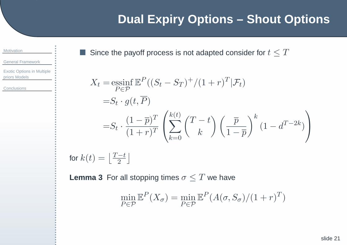
Since the payoff process is not adapted consider for t ≤ T

Xt =essinfP∈P

EP ((St − ST )

+/(1 + r)T |Ft)

=St · g(t, P )

=St ·(1− p)T

(1 + r)T

k(t)∑

k=0

(

T − t

k

)(

p

1− p

)k

(1− dT−2k)

for k(t) =⌊

T−t2

⌋

Lemma 3 For all stopping times σ ≤ T we have

minP∈P

EP (Xσ) = min

P∈PEP (A(σ, Sσ)/(1 + r)T )

Dual Expiry Options – Shout Floor

Motivation

General Framework


Conclusions

slide 22

We can maximize X instead of the original payoff

As a consequence we have

UP0 = essinf

P∈PEP

(

essinfQ∈P

EQ((Sσ∗ − ST )

+|Fσ∗)

)

= minP∈P

EP(

Sσ∗ · g(σ∗, P ))

= EP(

Sσ∗ · g(σ∗, P ))

where σ∗ is optimal.

The worst-case measure is defined by

P (ǫt+1|Ft) =

p if σ∗ < tp else

Dual Expiry Options – Shout Floor

Motivation

General Framework


Conclusions

slide 23

Lemma 4 The optimal stopping time for the above problem is given by

σ∗ = inft ≥ 0 : f(t) = x∗

where

f(t) = g(t, P ) · (p · u+ (1− p) · d)t

and x∗ is the maximum of f on [0, T ]

Proof: Generalized parking method and Optional Sampling

Remarks

1. Closed form solutions require exact study of the monotonicity of f

2. 1− p ≥ (p · u+ (1− p) · d) is sufficient to have

σ∗ = 0

U–shaped Payoffs

Motivation

General Framework


Conclusions

slide 24

U–shaped payoffs consist of two monotone parts allowing to benefit

from change in the underlying independently of the direction of the

change

Often used as speculative instrument before important events

Figure 2: Payoff of Straddle

U–shaped Payoffs

Motivation

General Framework


Conclusions

slide 25

Up- and Down-movement can increase the value of the claim

Uncertainty does not vanish over time

Lemma 5 The value process is Markovian. For every t ≤ T the value function

v(t, ·) is quasi-convex and there exists a sequence (xt)t≤T s.t. v(t, ·)increases on xt > xt and decreases else.

Proof: Backward induction

Proof uses explicitly the binomial structure of the model

As a consequence we obtain

P (ǫt+1 = 1|Ft) =

p if St < xtp if St ≥ xt

U–shaped Payoffs

Motivation

General Framework


Conclusions

slide 26

The worst-case measure is mean-reverting (in a wider sense)

The drift changes every time S hits a barrier and can happen arbitrary

often

Fears of the decision maker are opposite to the market movement

Increments are not independent anymore

Idea: Use the generalized parking method again or upper and lower

bounds

Conclusions

Motivation

General Framework


Conclusions

slide 27

Conclusions

Motivation

General Framework


Conclusions

slide 28

Conclusions

A model of a multiple priors market provided

A method to evaluate options in imperfect markets proposed

Pricing measure for several classes of payoffs derived

Worst-case measure is path-dependent in general

The structure of the stopping times carries over in this model

This is, however, due to the model and not a general result

Future work

Motivation

General Framework


Conclusions

slide 29

Continuous-time analysis – Brownian motion setting

Infinite time modeling in continuous time

Allows for closed form solutions and comparative statics

Mathematical traps due to multiple measure structure

More modeling necessary to build a meaningful mathematical

model

Motivation

General Framework


Conclusions

slide 30

Thank you for your attention!

exotic options in multiple priors models - fields institute options in multiple priors models...

Documents