exhibiting - research institute for mathematical sciences
TRANSCRIPT

Soliton Equations exhibiting“Pfaffian Solutions”
早大理工 広田良吾 (Ryogo Hirota)早大理工 岩尾昌央 (Masataka Iwao)阪大基礎工 辻本諭 (Satoshi Tujimoto)
Soliton equations whose solutions are expressed by pfaffians are briefly discussed. In-cluded are “Discrete-time Toda equation”, “Modified Toda equation of BKP type”, thecoupled modified $\mathrm{K}\mathrm{d}\mathrm{V}$ equation and (
$\zeta \mathrm{C}\mathrm{o}\mathrm{u}\mathrm{p}\mathrm{l}\mathrm{e}\mathrm{d}$ modified equation of derivative type”etc. The B\"acklund transformation of the discrete BKP equation in biliner form is de-scribed in detail in Appendix.
1 IntroductionPfaffian is known as a square root of an anti-symmetric determinant of order $2\mathrm{n}$ :
$\det|a_{jk}|_{1\leq j},k\leq 2n=[pf(a_{1}, a_{2}, \cdots, a2n)]^{2}$ .
We have, for example, for $\mathrm{n}=1$
$=pf(a_{1,2}a)2$ .
Hence$pf(a_{1}, a_{2})=a12$ .
For $\mathrm{n}=2$ ,
$=[a_{12}a_{34^{-}}a13a24+a_{14}a_{23}]2$ .
Hence$pf(a_{1}, a_{2}, a_{3}, a_{4})=a_{12}a_{34^{-a_{13^{O}}}}24+a_{14}a_{23}$ .
A square root of a determinant of a matrix $M$ of order $\mathrm{n}$ which is a sum of a unit matrix$E$ and a product of anti-symmetric matrices $A$ and $B$ is expressed by a two-componentpfaffian:
$\det|E+A\cross B|=[pf(a1, a2, \cdots, on’ b1, b2, \cdots, bn)]^{2}$ ,
数理解析研究所講究録1170巻 2000年 23-34 23
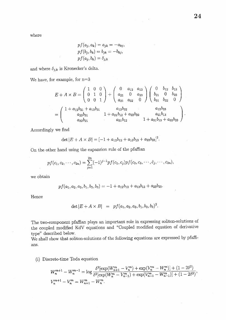
where
$pf(a_{j,k}a)=a_{j}k=-a_{kj}$ ,$pf(b_{j,k}b)=b_{jk}=-b_{k}j$ ,$pf(a_{j}, b_{k})=\delta_{j},k$
and where $\delta_{j,k}$ is Kronecker’s delta.
We have, for example, for $\mathrm{n}=3$
$E+A\cross B=+$$=$.
Accordingly we find
$\det|E+A\cross B|=[-1+a_{12}b_{12}+a_{13}b_{13}+a_{2\mathrm{s}^{b_{23}]^{2}}}$ .
On the other hand using the expansion rule of the pfaffian
$pf(C_{1}, C2, \cdots, c_{2n})=\sum_{j1}2n=(-1)j-1pf(c1, Cj)pf(C2, C3, \cdots,\hat{C}j)\ldots,2nc)$ ,
we obtain
$pf(a_{1}, a_{2,3}a, b_{1}, b2, b\mathrm{s})=-1+a12b_{12}+a_{13}b1\mathrm{s}+a23b_{23}$ .
Hence
$\det|E+\mathrm{A}\cross B|$ $=pf(a_{1}, a_{2,3,1,2,3}abbb)^{2}$ .
The two-component pfaffian plays an important role in expressing soliton-solutions of
the coupled modified $\mathrm{K}\mathrm{d}\mathrm{V}$ equations and “Coupled modified equation of derivativetype” described below.We shall show that soliton-solutions of the following equations are expressed by pfaffi-ans.
(i) Discrete-time Toda equation
$W_{n}^{m+1}-W_{n}m-1= \log\frac{\delta^{2}[\exp(Wm-V^{m})n+1n\mathrm{p}(+\mathrm{e}\mathrm{x}V_{n}^{m}-W_{n}m)]+(1-2\delta 2)}{\delta^{2}[\exp(Wm-nV_{n}^{m_{1}}-)+\exp(V_{n}m_{1^{-}}-W^{m}-1)n]+(1-2\delta^{2})}$ ,
$V_{n}^{m+1}-V^{m}=W_{n+1}nm-W^{m}n$ .
24

(ii) Modified Toda equation of BKP type
$\frac{d}{dt}\log\frac{\beta+V_{n}}{\beta-\alpha(In+I_{n-1})}=I_{n}-I_{n+1}$ ,
$\frac{d}{dt}I_{n}=V_{n-}1-V_{n}$ .
(iii) Coupled modified $\mathrm{K}\mathrm{d}\mathrm{V}$ equation
$\frac{\partial}{\partial t}v_{j}+6[\sum_{1\leq j<k\leq N}c_{j},kvjvk]\frac{\partial v_{j}}{\partial x}+\frac{\partial^{3}v_{j}}{\partial x^{3}}=0$ , $j=1,2,$ $\ldots,$$N$.
(iv) Coupled modified $\mathrm{K}\mathrm{d}\mathrm{V}$ equations of ($‘ \mathrm{d}\mathrm{e}\mathrm{r}\mathrm{i}\mathrm{v}\mathrm{a}\mathrm{t}\mathrm{i}\mathrm{v}\mathrm{e}$ type”
$\frac{\partial}{\partial t}v_{j}+6[\sum_{1\leq j<k\leq N}c_{j,k}D_{x}vj. v_{k}]\frac{\partial v_{j}}{\partial x}+\frac{\partial^{3}v_{j}}{\partial x^{3}}=0$ , $j=1,2,$ $\ldots,$$N$ .
We have the discrete KP equation
$[z_{1}\exp(D_{1})+z_{2}\exp(D2)+z_{\mathrm{s}}\exp(D3)]f\cdot f=0$
where $D_{1},$ $D_{2)}D_{3}$ and $z_{1},$ $z_{2,3}Z$ are bilinear operators and constants,respectively.Soliton solutions to the KP equation are known to be expressed by determinants [1].While the discrete BKP equation is expressed by
$[z_{1}\exp(D1)+z_{2}\exp(D2)+z_{3}\exp(D\mathrm{s})+z_{4}\exp(D_{4})]f\cdot f=0$
where $D_{1},$ $D_{2},$ $D_{3},$ $D_{4}$ and $z_{1},$ $z_{2},$ $Z_{3,4}Z$ are bilinear operators and constants, respectively,satisfying the relations
$D_{1}+D_{2}+D_{3}+D_{4}$ $=$ $0$ ,$z_{1}+z_{2}+Z3+z_{4}$ $=$ $0$ .
Solutions to the discrete BKP equation are well parametrized by parameters a,b and$\mathrm{c}$ which are the intervals of the coordinates $l,$ $m,$ $n[2]$ . We rewrite the discrete BKPequation using these parameters:
$(a+b)(a+c)(b-c)_{\mathcal{T}(\iota+1,m},$ $n)\mathcal{T}(l, m+1, n+1)$
$+(b+c)(b+a)(c-a)\mathcal{T}(\iota, m+1, n)\mathcal{T}(\iota+1, m, n+1)$
$+(C+a)(c+b)(a-b)_{\mathcal{T}}(\iota, m, n+1)_{\mathcal{T}}(l+1, m+1, n)$
$+(a-b)(b-c)(c-a)_{\mathcal{T}}(l, m, n)\tau(l+1, m+1, n+1)=0$.
Solutions are expressed by the pfaffian $[2],[3]$ :
$\tau(l, m, n)=pf(1,2,3, \cdots, 2N)$ ,
where the elements of the pfaffian are
$pf(j, k)\equiv cj,k$
$+ \sum_{\infty s=-}^{n-1}[\phi_{j(1}l, m, s+)\phi_{k}(l, m, S)-\phi_{j(}\iota, m, s)\phi k(\iota, m, S+1)]$
25

and $\phi_{j}(l, m, n)$ are a linear combination of (($\mathrm{e}\mathrm{x}\mathrm{p}\mathrm{o}\mathrm{n}\mathrm{e}\mathrm{n}\mathrm{t}\mathrm{i}\mathrm{a}\mathrm{l}$ functions in discrete space”
$( \frac{1-ap_{\mu}}{1+ap_{\mu}})^{l}(\frac{1-bp_{\mu}}{1+bp_{\mu}})^{m}(\frac{1-cp_{\mu}}{1+cp_{\mu}})^{n}$ ,
namely$\phi_{j}(l, m, n)=\sum_{\mu}\alpha_{j}\mu(\frac{1-ap_{\mu}}{1+ap_{\mu}})\iota(\frac{1-bp_{\mu}}{1+bp_{\mu}})^{m}(\frac{1-cp_{\mu}}{1+cp_{\mu}})^{n}$.
2 Soliton Equations Generated by the Bilinear BKPEquation
The followings are well-known soliton equations generated by the discrete BKP equa-tion.
(a) Sawada-Kotera equation
$D_{x}(D_{t}+D\overline{\mathrm{i})})xf\cdot f=0$,
$u=2 \frac{\partial^{2}}{\partial x^{2}}\log f$ ,
$u_{t}+15(u^{3}+uuxx)_{x}+u_{x}xxxx=0$ .
(b) Model equation of shallow-water wave
$D_{x}(D_{t}-D_{t}D_{x}^{2}+D_{x})f\dot{f}=0$ ,
$u=2 \frac{\partial^{2}}{\partial x^{2}}\log f$ ,
$u_{txt}-u_{x}-3uu_{t}+3u_{x} \int_{x}^{\infty}u_{t}dx’=0$ .
Here we add two more examples.(1) Discrete-time Toda equation.Let
$D_{1}$ $=$ $\frac{3}{2}\delta D_{t}$ , $z_{1}=1$ ,
$D_{2}$ $=$ $- \frac{1}{2}\delta D_{t}$ , $z_{2}=-1+2\delta 2$ ,
$D_{3}$ $=$ $D_{n}- \frac{1}{2}\delta D_{t}$ , $z_{\mathrm{s}=}-\delta^{2}$ ,
$D_{4}$ $=$ $-D_{nt}- \frac{1}{2}\delta D$ , $z_{4}=-\delta^{2}$ .
Then$[e^{\delta D_{t}+} \frac{1}{2}\delta D_{t}+e-\delta D_{t}+\frac{1}{2}\delta D_{t}-2e^{-}\frac{1}{2}\delta D_{t}$
$- \delta^{2}(e^{D_{n}\frac{1}{2}\delta D_{t}}-+e^{-D_{n}-}\frac{1}{2}\delta Dt-2e^{-}\frac{1}{2}\delta Di)]f\cdot f=0$,
26

which is rewritten as
$\cosh\frac{1}{2}\delta D_{t}[\sinh 2_{\frac{1}{2}}\delta Dt-\delta 2\sinh 2_{\frac{1}{2}}Dn]f\cdot f=0$ . (1)
The bilinear form indicates that 1-soliton solution is the same as that of the discrete-time Toda equation
$[\sinh^{2_{\frac{1}{2}\delta}}D_{t}-\delta^{2}\sinh^{2_{\frac{1}{2}}}D_{n}]f\cdot f=0$ .
The bilinear equation(l) is transformed into the nonlinear difference-difference equationin the ordinary form
$W_{n}^{m+1}-W_{n}^{m}-1= \log\frac{\delta^{2}[\exp(W_{n+1}^{m}+V^{m})n+\exp(V_{n}m-W_{n}^{m})]+(1-2\delta^{2})}{\delta^{2}[\exp(W^{m}+V_{n-}m)n1+\exp(V_{n}m_{1^{-}}-W^{m}-1)n]+(1-2\delta^{2})}$ ,
$V_{n}^{m+1m}-V_{n}m=WW_{n}^{m}n+1^{-}$’
through a series of dependent variable transformations
$f_{n}^{m}=e^{\phi^{m}}n$ ,$\triangle_{m}\phi^{m}n=\tau^{m}n$
’
$\triangle_{n}\phi_{n}^{m}=S_{n}^{m}$ ,$\triangle_{m}S_{n}^{m}=W_{n}m$ ,$\triangle_{n}S_{n}^{m}=V_{n}m$ ,
where $\triangle$ is the forward difference operator defined by
$\triangle_{m}f_{n}^{m}=\delta^{-1}[f_{n}^{m+1}-f_{n}^{m}]$ ,$\triangle_{n}f_{n}^{m}=fn+1m-fnm$ .
(2) Modified Toda equation of BKP type.Let
$D_{1}$ $=$ $\frac{1}{2}(\delta D_{x}+\epsilon D_{y})$ , $z_{1}=1$ ,
$D_{2}$ $=$ $\frac{1}{2}(\delta D_{x}-\epsilon D_{y})$ , $z_{2}=-1+\beta\delta\epsilon$ ,
$D_{3}$ $=$ $-D_{n}- \frac{1}{2}(\delta Dx+\epsilon D_{y})$ , $z_{3}=-\alpha\in-\beta\delta\epsilon$ ,
$D_{4}$ $=$ $D_{n}- \frac{1}{2}(\delta D_{x}-\epsilon D_{y})$ , $z_{4}=\alpha\epsilon$ .
Then
$\{e^{\frac{1}{2}(D_{x}+\epsilon D_{y}}\delta)-e\frac{1}{2}(\delta D_{x}-\epsilon D)y$
$+ \alpha\epsilon[e^{D_{n^{-}}(\delta}\frac{1}{2}D_{x^{-}}\epsilon D)-e^{-})yn^{-\frac{1}{2}(\delta DD_{y}}x+\epsilon]D$
$+ \beta\delta\epsilon[e^{\frac{1}{2}}-\epsilon D_{y}-(\delta Dx)e^{-D}\frac{1}{2}(\delta D_{x}+\epsilon D)v]n^{-}\}f\cdot f=0$ ,
27

which is rewritten as
$\frac{2}{\delta\epsilon}\sinh\frac{1}{2}\delta D_{x}\sinh\frac{1}{2}\epsilon Dfyn$ . $f_{n}$
$- \alpha\frac{1}{\delta}e^{\epsilon}\mathrm{s}\mathrm{i}D_{y}\mathrm{n}\mathrm{h}\frac{1}{2}\delta Dxfn+1^{\cdot}fn-1$
$-\beta[e^{\frac{1}{2}()(\delta}\delta Dx+\epsilon Dyf_{n+1}\cdot fn-1-e^{\frac{1}{2}}fD_{x^{-}}\epsilon D_{y})n. f_{n}]=0$ .
In the limit of small $\delta,$ $\epsilon$ we have
$D_{x}D_{y}f_{n}\cdot fnx=\alpha Dfn+1^{\cdot}fn-1+\beta(f_{n}+1fn-1-f_{n}^{2})$ .
The bilinear equation is transformed into the ordinary form
$\frac{\partial}{\partial x}\log\frac{\beta+V_{n}}{\beta-\alpha(In+I_{n+1})}=I_{n}-I_{n+1}$,
$\frac{\partial}{\partial y}I_{n}=V_{n-}1-V_{n}$ ,
through the transformation
$f_{n}=e^{s_{n}}$ ,
$V_{n}= \frac{\partial^{2}}{\partial x\partial y}S_{n}$ ,
$I_{n}= \frac{\partial}{\partial x}(S_{n-}1^{-s)}n$
’
which we call “modified Toda equation of BKP type”. The bilinear form of the modifiedToda equation of BKP type
$D_{x}D_{y}f_{n}\cdot f_{n}=\alpha D_{x}f_{n+1}\cdot fn-1+\beta(f_{n}+1fn-1-f_{n}^{2})$ ,
suggests that a new equation may be obtained by replacing the term
$f_{n+1}f_{n-}1-f_{n}^{2}$
by$D_{x}f_{n+1}\cdot fn-1$ .
We shall replace the term $g_{j}g_{k}$ by $D_{x}g_{j}\cdot g_{k}$ in order to obtain a coupled modified $\mathrm{K}\mathrm{d}\mathrm{V}$
equation of ($‘ \mathrm{d}\mathrm{e}\mathrm{r}\mathrm{i}\mathrm{v}\mathrm{a}\mathrm{t}\mathrm{i}_{\mathrm{V}}\mathrm{e}$ type”.
The well-known modified $\mathrm{K}\mathrm{d}\mathrm{V}$ equation
$\frac{\partial}{\partial t}v+6v^{2_{\frac{\partial}{\partial x}v+}}\frac{\partial^{3}}{\partial x^{3}}v=0$ ,
is transformed into the bilinear form
$(D_{t}+D_{x}^{3})f\cdot \mathit{9}=0$ ,$D_{x}^{2}f\cdot f=2g^{2}$ ,
28

through the dependent variable transformation
$v= \frac{g}{f}$ .
A coupled modified $\mathrm{K}\mathrm{d}\mathrm{V}$ equation is obtained by considering the following coupledform of the modified $\mathrm{K}\mathrm{d}\mathrm{V}$ equations [4].
$\{$
$(D_{t}+D_{x}^{3})f\cdot g_{j}=0$ , for $j=1,2,$ $\cdots N$ , (2)$Dx^{2}f\cdot f=2\Sigma 1\leq j<k\leq NC_{j},k\mathit{9}jgk$ ,
which is transformed into the ordinary form
$\frac{\partial}{\partial t}v_{j}+6[1\leq j<\sum_{k\leq N}c_{j,k}vjv_{k}]\frac{\partial v_{j}}{\partial x}+\frac{\partial^{3}v_{j}}{\partial x^{3}}=0$,
through the transformation$v_{j}= \frac{g_{j}}{f}$ .
The multisoliton solution to $\mathrm{e}\mathrm{q}.(2)$ is expressed by ($‘ \mathrm{t}\mathrm{w}\mathrm{o}$-component pfaffians” [4]:
$f=pf(a_{1}, a2, \cdots, a_{L}, b1, b_{2}, \cdots, b_{L})$ ,$g_{j}=pf(d_{0}, a_{1}, a_{2}, \cdots, a_{L}, b_{1}, b_{2}, \cdot .., b_{L}, c_{j})$ , for $j=1,2,$ $\cdots,$
$N$,
where the elements of pfaffians are defined as follows
$pf( \delta_{n’ \mathcal{U}}a)\equiv\frac{\partial^{n}}{\partial x^{n}}\exp(\eta_{\nu})$ , for $n=1,2,3,$ $\ldots$ ,
$pf(a_{\mu’\nu}a) \equiv\frac{p_{\mu}-p_{\nu}}{p_{\mu}+p_{\nu}}\exp(\eta_{\mu}+\eta_{\nu})$ ,
$pf(a_{\mu}, b_{\mathcal{U}})\equiv\delta_{\mu},\nu$
’
$pf(b_{\mu’\nu}b) \equiv-\frac{c_{j}k}{p_{\mu}^{2}-p_{\nu}^{2}}\exp(\eta_{\mu}+\eta_{\overline{\nu}})$ ,
$pf(b_{\mu}, c_{j})\equiv\{$1, if $b_{\mu}\in B_{j}$ ,$0$ , if $b_{l\text{ノ}}\not\in B_{k}$
$pf(otherwi_{S}e)\equiv 0$ .
A coupled modified $\mathrm{K}\mathrm{d}\mathrm{V}$ equation of ($‘ \mathrm{d}\mathrm{e}\mathrm{r}\mathrm{i}\mathrm{v}\mathrm{a}\mathrm{t}\mathrm{i}\mathrm{v}\mathrm{e}$ type” is obtained by replacing the
coupling terms of product form
$c_{jk}g_{j}gk$ , $(cjk=ckj)$
by coupling terms of derivative type
$cjkDxgj.\mathit{9}k$ , $(_{C_{jk}}=-C_{k}j)$ .
29
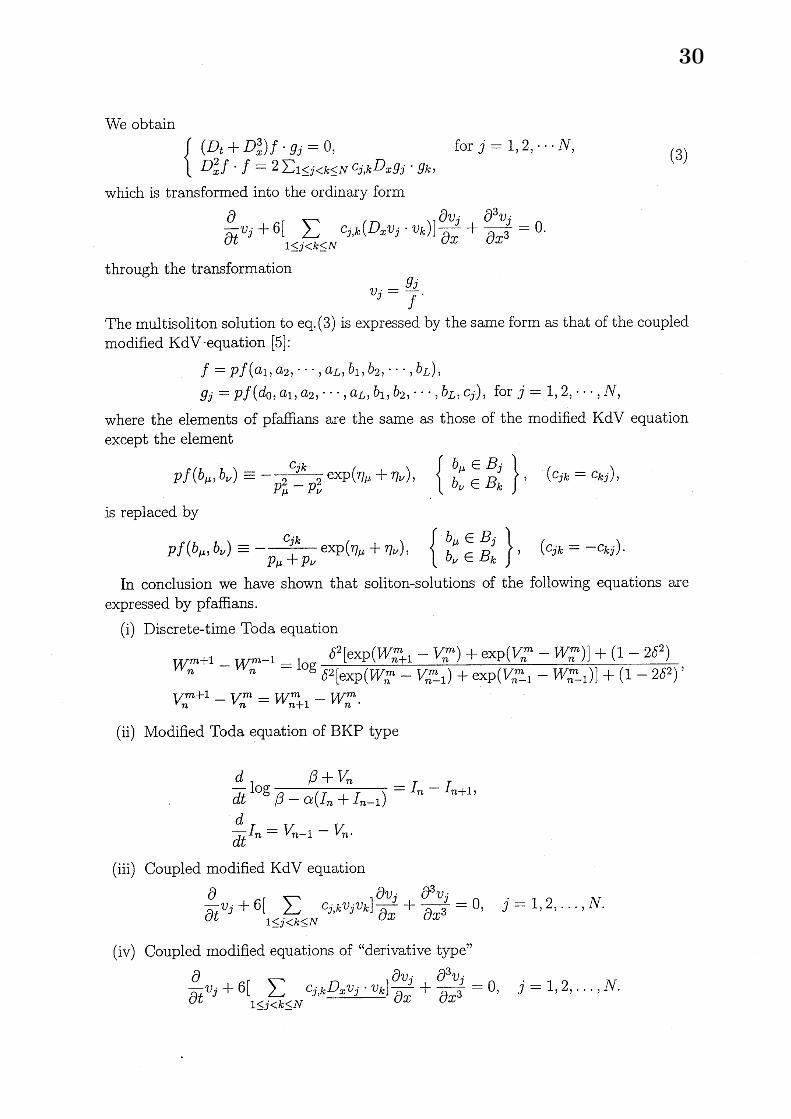
We obtain
$\{$
$(D_{t}+D_{x}^{3})f\cdot g_{j}=0$ , for $j=1,2,$ $\cdots N$ ,$D_{x}^{2}f\cdot f=2\Sigma 1\leq j<k\leq NC_{j,x}kDgj$ .
$g_{k}$ ,(3)
which is transformed into the ordinary form
$\frac{\partial}{\partial t}v_{j}+6[\sum_{1\leq j<k\leq N}c_{j},k(D_{x}vj.v_{k})]\frac{\partial v_{j}}{\partial x}+\frac{\partial^{3}v_{j}}{\partial x^{3}}=0$ .
through the transformation$v_{j}= \frac{g_{j}}{f}$ .
The multisoliton solution to $\mathrm{e}\mathrm{q}.(3)$ is expressed by the same form as that of the coupledmodified $\mathrm{K}\mathrm{d}\mathrm{V}\cdot \mathrm{e}\mathrm{q}\mathrm{u}\mathrm{a}\mathrm{t}\mathrm{i}\mathrm{o}\mathrm{n}[5]$ :
$f=pf(a_{1}, a_{2}, \cdots, a_{L}, b1, b_{2}, \cdots, b_{L})$ ,$g_{j}=pf(d_{0,1}a, a2, \cdots, a_{L,1}b, b2, \cdots, bL, cj)$ , for $j=1,2,$ $\cdots,$
$N$ ,
where the elements of pfaffians are the same as those of the modified $\mathrm{K}\mathrm{d}\mathrm{V}$ equationexcept the element
$pf(b_{\mu’\nu}b) \equiv-\frac{c_{jk}}{p_{\mu}^{2}-p_{\nu}^{2}}\exp(\eta_{\mu}+\eta_{\nu})$, $)$ $(C_{jk}=Ckj)$ ,
is replaced by
$pf(b_{\mu}, b_{\nu}) \equiv-\frac{c_{jk}}{p_{\mu}+p_{\nu}}\exp(\eta_{\mu}+\eta_{\nu})$ ,
In conclusion we have shown that soliton-solutions of the following equations areexpressed by pfaffians.
(i) Discrete-time Toda equation
$W_{n}^{m+1}-W_{n}m-1= \log\frac{\delta^{2}[\exp(W_{n}mV+1^{-}nm)+\exp(V_{n}m-W_{n}m)]+(1-2\delta^{2})}{\delta^{2}[\exp(W^{m}-nV_{n-}m)1+\exp(V_{n}m_{1^{-}}-W^{m}-1)n]+(1-2\delta^{2})}$ ,
$V_{n}^{m+1}-V_{n}m=Wm-n+1W_{n}^{m}$ .
(ii) Modified Toda equation of BKP type
$\frac{d}{dt}\log\frac{\beta+V_{n}}{\beta-\alpha(In+I_{n-1})}=In-I_{n+1}$ ,
$\frac{d}{dt}I_{n}=V_{n}-1^{-}V_{n}$ .
(iii) Coupled modified $\mathrm{K}\mathrm{d}\mathrm{V}$ equation
$\frac{\partial}{\partial t}v_{j}+6[\sum_{1\leq j<k\leq N}c_{j,k}vjvk]\frac{\partial v_{j}}{\partial x}+\frac{\partial^{3}v_{j}}{\partial x^{3}}=0$ , $j=1,2,$ $\ldots,$$N$ .
(iv) Coupled modified equations of “derivative type”
$\frac{\partial}{\partial t}v_{j}+6[1\leq jk\leq N\sum_{<}cj,k\underline{Dxjv\cdot vk}]\frac{\partial v_{j}}{\partial x}+\frac{\partial^{3}v_{j}}{\partial x^{3}}=0$, $j=1,2,$ $\ldots,$$N$ .
30

AB\"acklund $\mathrm{n}\mathrm{a}\mathrm{n}\mathrm{S}\mathrm{f}\mathrm{o}\mathrm{r}\mathrm{m}\mathrm{a}\mathrm{t}\mathrm{i}_{\mathrm{o}\mathrm{n}}$ of the Discrete BKPEquation
In this appendix we describe in detail how to obtain the B\"acklund transformation ofthe discrete BKP equation in bilinear form.The B\"acklund transformation which relates a solution $f$ of the discrete BKP euqation
$[z_{1}\exp(D1)+z_{2}\exp(D2)+z_{3}\exp(D3)+z_{4}\exp(D4)]f\cdot f=0$
with another solution $f’$ of the same equation
$[z_{1}\exp(D_{1})+z_{2}\exp(D_{2})+Z_{3}\exp(D_{3})+z4\exp(D4)]f’\cdot f/=0$
is obtained by considering the following quantity $P$
$P=\{[z_{1}\exp(D1)+z_{2}\exp(D2)+z_{3}\exp(D3)+z_{4}\exp(D4)]f\cdot f\}$
$\cross\{[z_{3}\exp(D3)+z_{4}\exp(D_{4})]f’\cdot f’\}$
$-\{[z_{3}\exp(D3)+z_{4}\exp(D4)]f\cdot f\}$
$\cross\{[z_{1}\exp(D1)+Z_{2}\exp(D_{2})+Z3\exp(D_{3})+Z_{4}\exp(D_{4})]f/. f’\}$
$=0$
and using the exchange formula$(e^{D_{1}}f \cdot f)(e^{D\prime}f3. f’)=e^{\frac{1}{2}()}[D1+D_{3}e^{\frac{1}{2}(}D_{1}-D_{3})f\cdot f’]\cdot[e-\frac{1}{2}(D_{1}-D_{3})f\cdot f’]$. (4)
In fact we find
$(e^{D_{1}}f\cdot f)(eD3f’\cdot f’)-(eD1f’\cdot f’)(e^{D_{3}}f\cdot f)$
$=e^{\frac{1}{2}()} \{D_{1}+D_{3}[e^{\frac{1}{2}(D-D_{3}}f1). f’]\cdot[e-\frac{1}{2}(D_{1}-D_{3})f\cdot f’]-[e-\frac{1}{2}(D_{1}-D3)f\cdot f’]\cdot[e^{\frac{1}{2}(D_{3}}-)fD1\}$
$=2 \sinh\frac{1}{2}(D_{1}+D_{3})[e\frac{1}{2}(D1-D_{3})f\cdot f/]\cdot[e-\frac{1}{2}(D1-D_{3})f\cdot f/]$ . (5)
Using $\mathrm{e}\mathrm{q}(5)$ and noting that $D_{1}+D_{2}+D_{3}+D_{4}=0$ we rewrite $P$ as
$P=2_{Z_{13}}z \sinh\frac{1}{2}(D_{1}+D_{3})[e^{\frac{1}{2}}(D1-D_{3})f\cdot f’]\cdot[e^{-\frac{1}{2}(-}D_{1}D\mathrm{s})f\cdot f’]$
$-2z_{24}Z \sinh\frac{1}{2}(D_{1}+D_{3})[e^{\frac{1}{2}(-D_{4})}D2f\cdot f’]\cdot[e-\frac{1}{2}(D2-D_{4})f\cdot f’]$
$-2_{Z_{1^{Z}4}} \sinh\frac{1}{2}(D_{2}+D3)[e\frac{1}{2}(D_{1}-D_{4})f\cdot f/]\cdot[e^{-(D_{1}}\frac{1}{2}-D_{4})f\cdot f’]$
+2$Z_{2}Z3 \sinh\frac{1}{2}(D_{2}+D_{3})[e\frac{1}{2}(D2-D_{3})f\cdot f/]\cdot[e-\frac{1}{2}(D_{2}-D_{3})f\cdot f’]$
$=2 \sinh\frac{1}{2}(D_{1}+D_{3})$
$\{z_{1^{Z_{3}[}}e^{\frac{1}{2}}-D_{3})f(D_{1}$ . $f’$ ] $\cdot[e-\frac{1}{2}(D_{1}-D_{3})f\cdot f’]$
$-z_{2}z_{4}[e \frac{1}{2}(D_{2}-D_{4})f\cdot f’]\cdot[e-\frac{1}{2}(D_{2}-D_{4})f\cdot f’]\}$
+2 $\sinh\frac{1}{2}(D_{2}+D_{3})$
$\{z_{2^{Z_{3}[}}e^{\frac{1}{2}}(D_{2}-D_{3})f\cdot f’]\cdot[e^{-(}\frac{1}{2}D_{2}-D_{3})f\cdot f/]$
$-z_{1}z_{4}[e \frac{1}{2}(D1-D_{4})f\cdot f’]\cdot[e^{-}\frac{1}{2}(D1-D4)f\cdot f’]\}$.
31

Here we conjecture that the following equations constitute the B\"acklund transformationof the discrete BKP equation
$[a_{1} \exp(\frac{1}{2}(D_{1^{-D_{3}))}}+a_{2}\exp(-\frac{1}{2}(D1-D\mathrm{s}))$
$+a_{3} \exp(\frac{1}{2}(D_{2^{-D_{4}))}}+a_{4}\exp(-\frac{1}{2}(D2-D_{4}))]f\cdot f’=0,$ $(6)$
$[b_{1} \exp(\frac{1}{2}(D_{2^{-}}D_{\mathrm{s}}))+b_{2}\exp(-\frac{1}{2}(D_{2^{-D_{3}))}}$
$+b_{3} \exp(\frac{1}{2}(D1-D_{4}))+b_{4}\exp(-\frac{1}{2}(D1^{-}D_{4}))]f\cdot f’=0$ , (7)
where new parameters $a_{1},$ $a_{2},$ $a_{3,41,2}a,$$bb,$ $b_{3}$ and $b_{4}$ are to be determined.Using $\mathrm{e}\mathrm{q}.(6)$ we have
$\sinh\frac{1}{2}(D_{1}+D3)$
$\{[a_{1}\exp(\frac{1}{2}(D_{1^{-D_{3}))}}+a_{4}\exp(-\frac{1}{2}(D2^{-}D_{4})]f\cdot f’\}$
$. \{[a_{2}\exp(-\frac{1}{2}(D_{1^{-D_{3}))}}+a_{3}\exp(\frac{1}{2}(D_{2}-D_{4})]f\cdot f’\}=0$
which gives a relation
$\sinh\frac{1}{2}(D_{1}+D3)$
$\{a_{1}a_{2}[\exp(\frac{1}{2}(D1-D_{3}))f\cdot f’]\cdot[\exp(-\frac{1}{2}(D_{1}-D_{3}))f\cdot f^{J}]$
$-a_{3}a_{4}[ \exp(\frac{1}{2}(D2^{-D_{4})})f\cdot f’]\cdot[\exp(-\frac{1}{2}(D_{2^{-}}D4))f\cdot f’]\}$
$= \sinh\frac{1}{2}(D_{1}+D3)$
$\{a_{1}a_{3}[\exp(\frac{1}{2}(D1^{-}D_{3}))f\cdot f’]\cdot[\exp(\frac{1}{2}(D2^{-D_{4}}))f\cdot f/]$
$-a_{2}a_{4}[ \exp(-\frac{1}{2}(D1-D_{3}))f\cdot f/]\cdot[\exp(-\frac{1}{2}(D_{2}-D_{4}))f\cdot f’]\}$ . (8)
We chose the following relations between the parameters
$\underline{Z_{1}Z_{3}}\underline{z2Z}=4=k1$ , (9)$a_{1}a_{2}$ $a_{3}a_{4}$
$\frac{z_{2}z_{3}}{b_{1}b_{2}}=\frac{z_{1}z_{4}}{b_{3}b_{4}}=k_{2}$. (10)
Then we find
$P=2k_{1} \sinh\frac{1}{2}(D_{1}+D_{3})$
$\{a_{1}a2[e^{\frac{1}{2}(}-D_{3})fD_{1}. f’]\cdot[e^{-\frac{1}{2}}-D3f(D1). f’]-a_{3}a4[e\frac{1}{2}(D_{2}-D_{4})f\cdot f’]\cdot[e^{-(DD_{4}}\frac{1}{2}2-)f\cdot f’]\}$
+2$k_{2} \sinh\frac{1}{2}(D_{2}+D_{3})$
$\{b_{1}b_{2}[e\frac{1}{2}(D_{2}-D_{3})f\cdot f/]\cdot[e^{-(-D_{3}}\frac{1}{2}D_{2})f\cdot f’]-b_{3}b_{4}[e\frac{1}{2}(D_{1}-D_{4})f\cdot f’]\cdot[e^{-(D}\frac{1}{2}1-D_{4})f\cdot f/]\}$ ,
32

which is, by using $\mathrm{e}\mathrm{q}.(8),\mathrm{r}\mathrm{e}\mathrm{w}\mathrm{r}\mathrm{i}\mathrm{t}\mathrm{t}\mathrm{e}\mathrm{n}$ as
$P=2k_{1} \sinh\frac{1}{2}(D_{1}+D_{3})$
$\{a_{1}a_{3}[e^{\frac{1}{2}}-3)f(D1D. f;]\cdot[e\frac{1}{2}(D2-D_{4})f\cdot f’]-a_{2}a_{4}[e-\frac{1}{2}(D_{1}-D_{3})f\cdot f’]\cdot[e-\frac{1}{2}(D_{2}-D_{4})f\cdot f’]\}$
$+2k_{2} \sinh\frac{1}{2}(D_{2}+D_{3})$
$\{b_{1}b_{3}[e\frac{1}{2}(D_{2}-D_{3})f\cdot f’]\cdot[e\frac{1}{2}(D1-D_{4})f\cdot f’]-b2b_{4}[e-\frac{1}{2}(D2-D3)f\cdot f’]\cdot[e^{-(}\frac{1}{2}D_{1}-D_{4})f\cdot f/]\}$ .
On the other hand we have the operator identy$e^{\frac{1}{2}()}D_{1}+D3[e \frac{1}{2}(D1-D_{3})f\cdot f^{J}]\cdot[e^{\frac{1}{2}(-D_{4}}fD_{2}). f^{J}]$
$=e^{\frac{1}{2}()}[D_{2}+D_{3}-D_{3})e^{\frac{1}{2}(D_{2}}f . f’]$ . $[e^{\frac{1}{2}(D_{1}-D_{4}})f . f’]$ . (11)
Using the identiy(ll) we obtain
$P=2 \sinh\frac{1}{2}(D_{1}+D_{3})$
$\{(k_{1}a_{1}a_{3}+k_{2}b_{1}b_{3})[e^{\frac{\mathrm{i}}{2}(D-D_{3}}f1). f’]\cdot[e^{\frac{1}{2}(D_{2}-D_{4}}f)f’]$
$-(k_{1}a_{2}a_{4}+k_{2}b_{2}b_{4})[e- \frac{1}{2}(D1-D_{3})f\cdot f’]\cdot[e^{-\frac{1}{2}()}-D4fD_{2}f’]\}$ ,
which vanishes if
$k_{1}a_{1}a_{3}+k_{2}b_{1}b_{3}=0$ , (12)$k_{1}a_{2}a_{4}+k_{2}b_{2}b_{4}=0$.
Substituting $\mathrm{e}\mathrm{q}_{\mathrm{S}}.(9)$ and (10) into the above relations we find that they are satisfied if
$z_{1}a_{3}b_{2}+z_{2}a_{2}b_{3}=0$ . (13)
Hence the B\"acklund transformation of the discrete BKP equation are given by
$[a_{1} \exp(\frac{1}{2}(D_{1^{-D_{3}))}}+a_{2}\exp(-\frac{1}{2}(D_{1^{-D_{3}))}}$
$+a_{3} \exp(\frac{1}{2}(D_{2^{-D_{4}))}}+a_{4}\exp(-\frac{1}{2}(D_{2^{-}}D_{4}))]f\cdot fJ=0,$ (14)
$[b_{1} \exp(\frac{1}{2}(D2-D_{3}))+b_{2}\exp(-\frac{1}{2}(D_{2}-D_{3}))$
$+b_{3} \exp(\frac{1}{2}(D_{1^{-D_{4}))}}+b_{4}\exp(-\frac{1}{2}(D_{1^{-}}D_{4}))]f\cdot fJ=0,$ (15)
provided that parameters satisfy the relations
$z_{1}z_{3}a_{3}a4-z2Z4a1a2$ $=$ $0$ ,$z_{2}z_{334^{-Z_{1}}}bbz_{4}b_{1}b2$ $=$ $0$ ,
$z_{2}a_{2}b_{3}+z1a_{\mathrm{s}}b_{2}$ $=$ $0$ .
Finally we note that equations (14) and (15) exhibit soliton solutions provided thatthe parameters $\mathrm{s}\mathrm{a}\mathrm{t}\mathrm{i}\mathrm{s}\Phi$ the conditions
$a_{1}+a_{2}+a_{3}+a_{4}$ $=$ $0$ ,$b_{1}+b_{2}+b_{3}+b4$ $=$ $0$ .
33

References[1] Y.Ohta, R.Hirota, S.Tujimoto and T.Imai, ((Casorati and Discrete Gram Type De-
terminant Representations of Solutions to the Discrete KP Hierarchy in BilinearForm”, J.Phy.Soc.Jpn. 62 (1993) 1872.
[2] T. Miwa, Proc.Jpn.Acad. $58\mathrm{A}(1\mathit{9}82)$ 9.
[3] Satoshi Tsujimoto and Ryogo Hirota, $‘(\mathrm{P}\mathrm{f}\mathrm{a}\mathrm{f}\mathrm{f}\mathrm{i}\mathrm{a}\mathrm{n}$ Representation of Solutions to theDiscrete BKP Hierarchy in Bilinear Form”, J.Phy.Soc.Jpn. 65 (1996) 2797.
[4] Masataka Iwao and Ryogo Hirota,(( $\mathrm{S}_{0}1\mathrm{i}\mathrm{t}\mathrm{o}\mathrm{n}$ Solution of a Coupled Modified KdVEquation,J.Phy.Soc.Jpn. 66 (1997) 577.
[5] Masataka Iwao and Ryogo Hirota, “Soliton Solution of a Coupled Derivative Mod-ified KdV Equation, to appear in J.Phy.Soc.Jpn.
34