exercise: frequency response...
TRANSCRIPT
ControlEngineering
UniversityCollegeofSoutheastNorway
http://home.hit.no/~hansha
Exercise:FrequencyResponse(Solutions)
Introduction
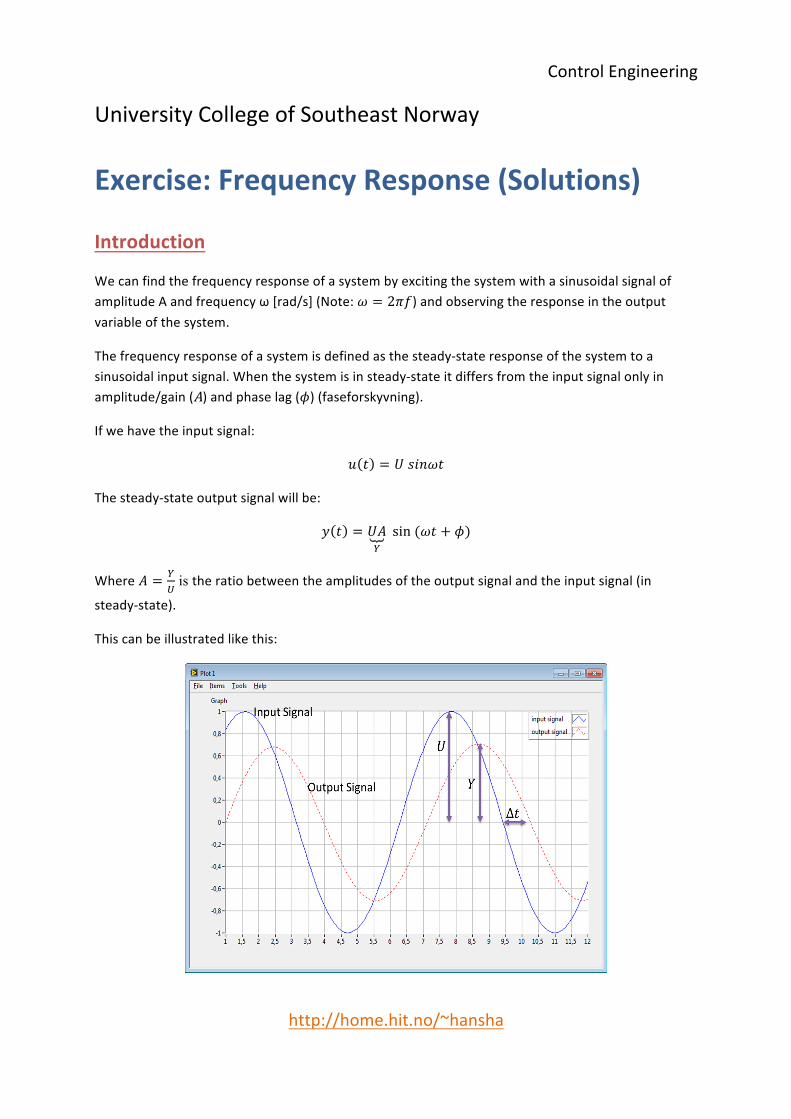
WecanfindthefrequencyresponseofasystembyexcitingthesystemwithasinusoidalsignalofamplitudeAandfrequencyω[rad/s](Note:𝜔 = 2𝜋𝑓)andobservingtheresponseintheoutputvariableofthesystem.
Thefrequencyresponseofasystemisdefinedasthesteady-stateresponseofthesystemtoasinusoidalinputsignal.Whenthesystemisinsteady-stateitdiffersfromtheinputsignalonlyinamplitude/gain(A)andphaselag(𝜙)(faseforskyvning).
Ifwehavetheinputsignal:
𝑢 𝑡 = 𝑈𝑠𝑖𝑛𝜔𝑡
Thesteady-stateoutputsignalwillbe:
𝑦 𝑡 = 𝑈𝐴1sin(𝜔𝑡 + 𝜙)
Where 𝐴 = 18
is theratiobetweentheamplitudesoftheoutputsignalandtheinputsignal(in
steady-state).
Thiscanbeillustratedlikethis:

2
ControlEngineering
Thegainisgivenby:
𝐴 =𝑌𝑈
Thephaselagisgivenby:
𝜙 = −𝜔Δ𝑡[𝑟𝑎𝑑]
FindtheFrequencyResponsefromtheTransferfunction
Aand𝜙isafunctionofthefrequency𝜔sowemaywrite𝐴 = 𝐴 𝜔 , 𝜙 = 𝜙(𝜔)
Foratransferfunction:
𝐻 𝑆 =𝑦(𝑠)𝑢(𝑠)
Wehavethat:
𝐻 𝑗𝜔 = 𝐻(𝑗𝜔) 𝑒N∠P(NQ)
Where𝐻(𝑗𝜔)isthefrequencyresponseofthesystem,i.e.,wemayfindthefrequencyresponsebysetting𝒔 = 𝒋𝝎inthetransferfunction.Bodediagramsareusefulinfrequencyresponseanalysis.
TheGainfunctionisdefinedas:
𝐴 𝜔 = 𝐻(𝑗𝜔)
ThePhasefunctionisdefinedas:
𝜙 𝜔 = ∠𝐻(𝑗𝜔)
Thiscanbeillustratedinthecomplexplanelikethis:

3
ControlEngineering
BodeDiagram
WenormallyuseaBodediagramtodrawthefrequencyresponseforagivensystem.TheBodediagramconsistsof2diagrams,theBodemagnitudediagram,𝐴(𝜔)andtheBodephasediagram,𝜙(𝜔).BelowweseeanexampleofaBodediagram:
The𝐴(𝜔)-axisisindecibel(dB),wherethedecibelvalueofxiscalculatedas:𝑥 𝑑𝐵 = 20𝑙𝑜𝑔[\𝑥
The𝜙(𝜔)-axisisindegrees(notradians!).Weuselogarithmicscaleonthe𝑥-axes.
ComplexNumbers
Acomplexnumberisdefinedlikethis:
𝑧 = 𝑎 + 𝑗𝑏
Theimaginaryunit𝑗isdefinedas:
𝑗 = −1
Where𝑎iscalledtherealpartof𝑧and𝑏iscalledtheimaginarypartof𝑧
𝑅𝑒(𝑧) = 𝑎,𝐼𝑚(𝑧) = 𝑏
Youmayalsoimaginarynumbersonexponential/polarform:
𝑧 = 𝑟𝑒Nc
Where:
𝑟 = 𝑧 = 𝑎d + 𝑏d

4
ControlEngineering
𝜃 = 𝑎𝑡𝑎𝑛𝑏𝑎
Notethat𝑎 = 𝑟 cos 𝜃and𝑏 = 𝑟 sin 𝜃
Rectangularformofacomplexnumber Exponential/polarformofacomplexnumber
[Figure:R.C.DorfandR.H.Bishop,ModernControlSystems,EleventhEdition:PearsonPrenticeHall]
MathScript
MathScripthasseveralbuilt-infunctionsforFrequencyresponse,e.g.:
Function Description Exampletf Createssystemmodelintransferfunctionform.Youalsocan
usethisfunctiontostate-spacemodelstotransferfunctionform.
>num=[1]; >den=[1, 1, 1]; >H = tf(num, den)
bode CreatestheBodemagnitudeandBodephaseplotsofasystemmodel.Youalsocanusethisfunctiontoreturnthemagnitudeandphasevaluesofamodelatfrequenciesyouspecify.Ifyoudonotspecifyanoutput,thisfunctioncreatesaplot.
>num=[4]; >den=[2, 1]; >H = tf(num, den) >bode(H)
bodemag CreatestheBodemagnitudeplotofasystemmodel.Ifyoudonotspecifyanoutput,thisfunctioncreatesaplot.
>[mag, wout] = bodemag(SysIn) >[mag, wout] = bodemag(SysIn, [wmin wmax]) >[mag, wout] = bodemag(SysIn, wlist)
semilogx Generatesaplotwithalogarithmicx-scale. >semilogx(w, gain)
log10 Computesthebase10logarithmoftheinputelements.Thebase10logarithmofzerois-inf.
>log(x)
atan Computesthearctangentofx >atan(x)
Example:
Wehavethefollowingtransferfunction:
𝐻 𝑠 =𝑦(𝑠)𝑢(𝑠)
=1
𝑠 + 1
BelowweseethescriptforcreatingthefrequencyresponseofthesysteminaBodeplotusingthebodefunctioninMathScript.Usethegridfunctiontoapplyagridtotheplot.
% We define the transfer function: K = 1;

5
ControlEngineering
T = 1; num = [K]; den = [T, 1]; H = tf(num, den) % We plot the Bode diagram: bode(H); % We add grid to the plot: subplot(2,1,1) grid on subplot(2,1,2) grid on
ThisgivesthefollowingBodeplot:
Task1:FrequencyResponse
Giventhefollowingsystem:
𝐻 𝑠 =4
2𝑠 + 1
1. Findthemathematicalexpressionsfor𝐴 𝜔 [𝑑𝐵]and𝜙(𝜔)using“pen&paper”.2. Findthebreakfrequencies(Norwegian:“knekkfrekvenser”)using“pen&paper”3. Findpolesandzeroesforthesystem(checkyouranswerusingMathScript)4. PlottheBodeplotusingMathScript
6
ControlEngineering
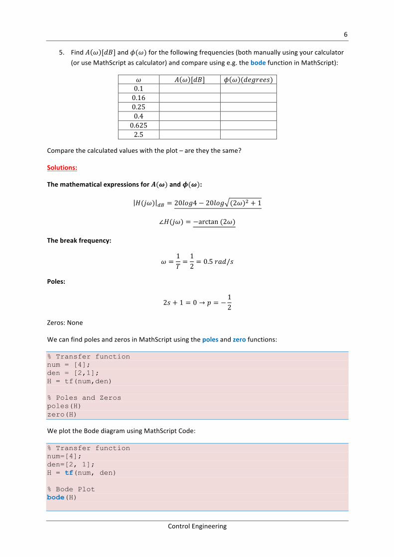
5. Find𝐴 𝜔 [𝑑𝐵]and𝜙(𝜔)forthefollowingfrequencies(bothmanuallyusingyourcalculator(oruseMathScriptascalculator)andcompareusinge.g.thebodefunctioninMathScript):
𝜔 𝐴 𝜔 [𝑑𝐵] 𝜙 𝜔 (𝑑𝑒𝑔𝑟𝑒𝑒𝑠)0.1 0.16 0.25 0.4 0.625 2.5
Comparethecalculatedvalueswiththeplot–aretheythesame?
Solutions:
Themathematicalexpressionsfor𝑨(𝝎)and𝝓(𝝎):
𝐻(𝑗𝜔) mn = 20𝑙𝑜𝑔4 − 20𝑙𝑜𝑔 (2𝜔)d + 1
∠𝐻(𝑗𝜔) = −arctan(2𝜔)
Thebreakfrequency:
𝜔 =1𝑇=12= 0.5𝑟𝑎𝑑/𝑠
Poles:
2𝑠 + 1 = 0 → 𝑝 = −12
Zeros:None
WecanfindpolesandzerosinMathScriptusingthepolesandzerofunctions:
% Transfer function num = [4]; den = [2,1]; H = tf(num,den) % Poles and Zeros poles(H) zero(H)
WeplottheBodediagramusingMathScriptCode:
% Transfer function num=[4]; den=[2, 1]; H = tf(num, den) % Bode Plot bode(H)
7
ControlEngineering
subplot(2,1,1) grid on subplot(2,1,2) grid on
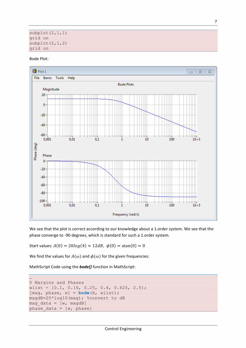
BodePlot:
Weseethattheplotiscorrectaccordingtoourknowledgeabouta1.ordersystem.Weseethatthephaseconvergeto-90degrees,whichisstandardforsucha1.ordersystem.
Startvalues:𝐴 0 = 20𝑙𝑜𝑔 4 ≈ 12𝑑𝐵, 𝜙 0 = atan 0 = 0
Wefindthevaluesfor𝐴(𝜔)and𝜙(𝜔)forthegivenfrequencies:
MathScriptCodeusingthebode()functioninMathScript:
… % Margins and Phases wlist = [0.1, 0.16, 0.25, 0.4, 0.625, 2.5]; [mag, phase, w] = bode(H, wlist); magdB=20*log10(mag); %convert to dB mag_data = [w, magdB] phase_data = [w, phase]

8
ControlEngineering
Thisgivesthefollowingresults:
𝜔 𝐴(𝜔) 𝜙(𝜔)0.1 11.9 -11.30.16 11.6 -17.70.25 11.1 -26.50.4 9.9 -38.70.625 7.8 -51.32.5 -2.1 -78.6
Alternatively,wecanusethemathematicalexpressionsfor𝐴(𝜔)and𝜙(𝜔):
gain = 20*log10(4) - 20*log10(sqrt((2*w).^2+1)); phase = -atan(2*w); phasedeg = phase * 180/pi; %convert to degrees
Theresultsisthesame.
Ifweuseacalculator,thisishowweneedtodoit.
Task2:BodeDiagrams
Dothefollowingforthesystemsgivenbelow.
1. Findthemathematicalexpressionsfor𝐴 𝜔 [𝑑𝐵]and𝜙(𝜔)using“pen&paper”.2. Findthebreakfrequencies(Norwegian:“knekkfrekvenser”)using“pen&paper”3. PlottheBodeplotusingMathScript(Usethebode()function)4. Findpolesandzeroesforthesystem(checkyouranswerusingMathScript)
Task2.1
Giventhefollowingtransferfunction:
𝐻 𝑆 =5
𝑠 + 1 (10𝑠 + 1)
Solutions:
Themathematicalexpressionsfor𝑨(𝝎)and𝝓(𝝎):
𝐻(𝑗𝜔) mn = 20𝑙𝑜𝑔5 − 20𝑙𝑜𝑔 (𝜔)d + 1 − 20𝑙𝑜𝑔 (10𝜔)d + 1
∠𝐻(𝑗𝜔) = −arctan(𝜔) − arctan(10𝜔)
Breakfrequencies:
𝜔[ =1𝑇[=11= 1𝑟𝑎𝑑/𝑠
𝜔d =1𝑇d=
110
= 0.1𝑟𝑎𝑑/𝑠

9
ControlEngineering
Bodeplot:
clear clc % Transfer function K = 5; T1 = 1; T2 = 10; num = [K]; den1 = [T1, 1]; den2 = [T2, 1]; den = conv(den1,den2); H = tf(num, den) % Bode Plot bode(H) subplot(2,1,1) grid on subplot(2,1,2) grid on
Note!Weusedthefunctionconvtocreatethedenominator,butwecouldalsodothismanually:
𝑠 + 1 10𝑠 + 1 = 10𝑠d + 𝑠 + 10𝑠 + 1 = 10𝑠d + 11𝑠 + 1
Thedenominatorcanthenbedefinedas:
den=[10, 11, 1]
Polesandzeroes:

10
ControlEngineering
𝑝[ = −1
𝑝d = −110
= −0.1
Nozeros.
UsethepolesandzerofunctionsinMathScript.
Task2.2
Giventhefollowingtransferfunction:
𝐻 𝑆 =1
𝑠 𝑠 + 1 d
Solutions:
Themathematicalexpressionsfor𝑨(𝝎)and𝝓(𝝎):
𝐻(𝑗𝜔) mn = −20𝑙𝑜𝑔 (𝜔)d − 2𝑥20𝑙𝑜𝑔 (𝜔)d + 1 = 20𝑙𝑜𝑔𝜔 − 40𝑙𝑜𝑔 (𝜔)d + 1
∠𝐻(𝑗𝜔) = −90 − 2arctan(𝜔)
Breakfrequencies:
𝜔 =1𝑇=11= 1𝑟𝑎𝑑/𝑠
Bodeplot:
clear clc % Transfer function num = [1]; den1 = [1, 0]; den2 = [1, 1]; den3 = [1, 1]; den = conv(den1,conv(den2,den3)); H = tf(num, den) % Bode Plot bode(H) subplot(2,1,1) grid on subplot(2,1,2) grid on

11
ControlEngineering
Polesandzeroes:
Poles:
𝑝[ = 0
𝑝d = −1
𝑝u = −1
Zeros:None
UsethepolesandzerofunctionsinMathScript.
Task2.3
Giventhefollowingtransferfunction:
𝐻 𝑠 =3.2𝑒wdx
3𝑠 + 1
Solutions:
Themathematicalexpressionsfor𝑨(𝝎)and𝝓(𝝎):
𝐻(𝑗𝜔) mn = 20𝑙𝑜𝑔3.2 − 20𝑙𝑜𝑔 (3𝜔)d + 1
∠𝐻(𝑗𝜔) = −2𝜔 − arctan(3𝜔)
Orindegrees:

12
ControlEngineering
∠𝐻 𝑗𝜔 = −2𝜔 − arctan(3𝜔) ∙180𝜋
Breakfrequencies:
𝜔 =1𝑇=13= 0.33𝑟𝑎𝑑/𝑠
Bodeplot:
MathScriptCode:
s=tf('s'); K=3.2; T=3; H1=tf(K/(T*s+1)); delay=2; H2=set(H1,'inputdelay',delay); bode(H2);
BodePlot:
Weseethattheplotiscorrectaccordingtoourknowledgeaboutasystemwithdelay.Weseethatthephasecurveisverysteep,whichisstandardforsuchasystem.
Polesandzeroes:
Poles:
𝑝[ = −13= −0.33
Zeros:None:
UsethepolesandzerofunctionsinMathScript.

13
ControlEngineering
Task2.4
Giventhefollowingtransferfunction:
𝐻 𝑆 =(5𝑠 + 1)
2𝑠 + 1 (10𝑠 + 1)
Solutions:
Themathematicalexpressionsfor𝑨(𝝎)and𝝓(𝝎):
𝐻(𝑗𝜔) mn = 20𝑙𝑜𝑔 (5𝜔)d + 1 − 20𝑙𝑜𝑔 (2𝜔)d + 1 − 20𝑙𝑜𝑔 (10𝜔)d + 1
∠𝐻(𝑗𝜔) = arctan(5𝜔) − arctan(2𝜔) − arctan(10𝜔)
Breakfrequencies:
𝜔[ =1𝑇[=15= 1𝑟𝑎𝑑/𝑠
𝜔d =1𝑇d=12= 0.5𝑟𝑎𝑑/𝑠
𝜔u =1𝑇u=
110
= 0.1𝑟𝑎𝑑/𝑠
Bodeplot:
clear clc % Transfer function num = [5, 1]; den1 = [2, 1]; den2 = [10, 1]; den = conv(den1,den2); H = tf(num, den) p = poles(H) z = zero(H) % Bode Plot bode(H) subplot(2,1,1) grid on subplot(2,1,2) grid on

14
ControlEngineering
Polesandzeroes:
p =
-0.1
-0.5
z =
-0.2
UsethepolesandzerofunctionsinMathScript.
Task3:Steady-stateResponse
Giventhefollowingsystem:
𝐻 𝑠 =𝑦(𝑠)𝑢(𝑠)
=1
𝑠 + 1
Thefrequencyresponseforthesystemisthen:

15
ControlEngineering
(YoumayuseMathScripttoseeifyougetthesamefrequencyresponse)
Foragiveninputsignal:
𝑢 𝑡 = 𝑈𝑠𝑖𝑛𝜔𝑡
Thesteady-stateoutputsignalwillbe:
𝑦 𝑡 = 𝑈𝐴𝑠𝑖𝑛(𝜔𝑡 + 𝜙)
Task3.1
Assumetheinputsignal𝑢tothesystemisasinusoidalwithamplitude𝑈 = 0.8andfrequency𝜔 =1.0𝑟𝑎𝑑/𝑠.
Findthesteady-stateoutputsignal.
Solution:
Thesteady-stateoutputsignalisdefinedas:
𝑦 𝑡 = 𝑈𝐴𝑠𝑖𝑛(𝜔𝑡 + 𝜙)
where𝑈 = 0.8
Wefind𝐴forfrequency𝜔 = 1.0𝑟𝑎𝑑/𝑠fromtheBodediagram:
𝐴 1.0 = −3𝑑𝐵
or:

16
ControlEngineering
𝐴 1.0 = 10wu/d\ = 0.71
(Note!𝑥 𝑑𝐵 = 20𝑙𝑜𝑔[\𝑥)
Thenwefind𝜙(1.0)fromtheBodediagram:
𝜙 1.0 = −45° = −45𝜋180
𝑟𝑎𝑑 = −0.79𝑟𝑎𝑑
(Note!2𝜋 𝑟𝑎𝑑𝑖𝑎𝑛𝑠 = 360[𝑑𝑒𝑔𝑟𝑒𝑒𝑠])
Thisgivesthefollowingsteady-stateoutputresponse:
𝑦 𝑡 = 𝑈𝐴𝑠𝑖𝑛(𝜔𝑡 + 𝜙)
Withvalues:
𝑦 𝑡 = 0.8 ∙ 0.71 ∙ 𝑠𝑖 𝑛 1.0 ∙ 𝑡 − 0.79
i.e.,steady-stateoutputresponsebecomes:
𝑦 𝑡 = 0.57𝑠𝑖𝑛(𝑡 − 0.79)
TheMathScriptcodeusedforcreatingthefrequencyresponse(Bodediagram)isasfollows:
% We define the transfer function: K = 1; T = 1; num = [K]; den = [T, 1]; H = tf(num, den) % We plot the Bode diagram: bode(H); % We add grid to the plot: subplot(2,1,1) grid on subplot(2,1,2) grid on
Task4:
Giventhefollowingtransferfunction:
𝐻 𝑠 =𝑦(𝑠)𝑢(𝑠)
=𝐾
(𝑇[𝑠 + 1)(𝑇d𝑠 + 1)
Task4.1
Findthemathematicalexpressionsfor𝐴(𝜔)and𝜙(𝜔)
Solution:

17
ControlEngineering
Wefindthefrequencyresponsebyreplacing𝑠with𝑗𝜔inourtransferfunction.Thismeanswehavetodealwithcomplexnumbers.
Shortintroductiontocomplexnumbers:
Acomplexnumberisdefinedlikethis:
𝑧 = 𝑎 + 𝑗𝑏
Theimaginaryunit𝑗isdefinedas:
𝑗 = −1
Where𝑎iscalledtherealpartof𝑧and𝑏iscalledtheimaginarypartof𝑧
𝑅𝑒(𝑧) = 𝑎,𝐼𝑚(𝑧) = 𝑏
Youmayalsoimaginarynumbersonexponential/polarform:
𝑧 = 𝑟𝑒Nc
Where:
𝑟 = 𝑧 = 𝑎d + 𝑏d
𝜃 = 𝑎𝑡𝑎𝑛𝑏𝑎
Notethat𝑎 = 𝑟 cos 𝜃and𝑏 = 𝑟 sin 𝜃
Rectangularformofacomplexnumber Exponential/polarformofacomplexnumber
[Figure:R.C.DorfandR.H.Bishop,ModernControlSystems,EleventhEdition:PearsonPrenticeHall]
Giventhecomplexnumbers:
𝑧[ = 𝑟[𝑒Nc~ and𝑧d = 𝑟d𝑒Nc�
Multiplication:

18
ControlEngineering
𝑧u = 𝑧[𝑧d = 𝑟[𝑟d𝑒N(c~�c�)
Division:
𝑧u =𝑧[𝑧d=𝑟[𝑒Nc~
𝑟d𝑒Nc�=𝑟[𝑟d𝑒N(c~wc�)
Thefrequencyresponseofthesystemisdefinedas:
𝐻 𝑗𝜔 = 𝐻(𝑗𝜔) 𝑒N∠P(NQ)
TheGainfunctionisdefinedas:
𝐴 𝜔 = 𝐻(𝑗𝜔)
ThePhasefunctionisdefinedas:
𝜙 𝜔 = ∠𝐻(𝑗𝜔)
Thefrequencyresponse(wereplace𝑠with𝑗𝜔)foroursystemthenbecomes:
𝐻 𝑗𝜔 =𝐾
(𝑇[𝑗𝜔 + 1)(𝑇d𝑗𝜔 + 1)
Onpolarform:
𝐻 𝑗𝜔 =𝐾
1d + 𝑇[𝜔 d𝑒N �������~Q[ 1d + 𝑇d𝜔 d𝑒N ������
��Q[
=𝐾
1 + 𝑇[𝜔 d 1 + 𝑇d𝜔 d𝑒N w������(�~Q)w������(��Q)
TheGainfunctionisdefinedas:
𝐴 𝜔 = 𝐻(𝑗𝜔) =𝐾
1 + 𝑇[𝜔 d 1 + 𝑇d𝜔 d
ThePhasefunctionisdefinedas:
𝜙 𝜔 = ∠𝐻 𝑗𝜔 = 𝑎𝑟𝑔 𝐻(𝑗𝜔) = −𝑎𝑟𝑐𝑡𝑎𝑛(𝑇[𝜔)−𝑎𝑟𝑐𝑡𝑎𝑛(𝑇d𝜔)
Task5:Sinusoidalinputandoutputsignals
Giventhefollowingplotofthesinusoidalinputandoutputsignalforagivensystem:

19
ControlEngineering
Theinputsignalisgivenby:
𝑢 𝑡 = 𝑈𝑠𝑖𝑛𝜔𝑡
Thesteady-stateoutputsignalwillthenbe:
𝑦 𝑡 = 𝑈𝐴1𝑠𝑖𝑛(𝜔𝑡 + 𝜙)
Thegainisgivenby:
𝐴 =𝑌𝑈
Thephaselagisgivenby:
𝜙 = −𝜔Δ𝑡[𝑟𝑎𝑑]
Task5.1
Whatisthefrequencyofthesignalin𝐻𝑧andin𝑟𝑎𝑑/𝑠?
Solution:
Fromthefigureweseethattheperiodoftheinputsignalis:
𝑇� = 6.2𝑠𝑒𝑐
(i.e.,7.8𝑠𝑒𝑐 − 1.6𝑠𝑒𝑐 = 6.2𝑠𝑒𝑐)
Thisgivesthefollowingfrequency:

20
ControlEngineering
𝑓 =1𝑇�=
16.2
= 0.16𝐻𝑧
or:
𝜔 = 2𝜋𝑓 = 2𝜋 ∙ 0.16 = 1𝑟𝑎𝑑/𝑠
Task5.2
Calculatetheamplitudegain(𝐴)andthephaselag(𝜙)atthefrequencyfoundinTask5.1.
WhatistheamplitudegainindB?Whatisthephaselagindegrees?
Solution:
Thegainisgivenby:
𝐴 =𝑌𝑈
Thephaselagisgivenby:
𝜙 = −𝜔Δ𝑡[𝑟𝑎𝑑]
Fromtheplotweget:
𝑈 = 1
𝑌 = 0.68
Δ𝑡 = 0.8
Thisgivesthefollowing:

21
ControlEngineering
Amplitudegain:
𝐴 =𝑌𝑈=0.681
= 0.68
OrindB:
𝐴 𝑑𝐵 = 20 log 0.68 = −3.35𝑑𝐵
Phaselag:
𝜙 = −𝜔Δ𝑡 = −1 ∙ 0.8 = −0.8𝑟𝑎𝑑
Orindegrees(2𝜋 𝑟𝑎𝑑 = 360°):
𝜙[𝑑𝑒𝑔𝑟𝑒𝑒𝑠] =180𝜋
∙ −0.8 = −45.9°
Task5.3
Whatisthesteady-stateoutputresponse?
Solution:
Thesteady-stateoutputresponseis:
𝑦 𝑡 = 𝑈𝐴𝑠𝑖𝑛(𝜔𝑡 + 𝜙)
Withvalues:
𝑦 𝑡 = 1 ∙ 0.68𝑠𝑖𝑛(1 ∙ 𝑡 − 0.8)
i.e.:
𝑦 𝑡 = 0.68𝑠𝑖𝑛(𝑡 − 0.8)
Task5.4
Thetransferfunctionforthesystemisactually:
𝐻 =1
𝑠 + 1
UseMathScripttoplottheBodediagram.
Fromtheplot,findtheamplitudegain(𝐴)andthephaselag(𝜙)atthefrequencyfoundinTask5.1.
Doyougetthesameresults?
Solution:
MathScriptCode:
clear

22
ControlEngineering
clc clf % Define Transfer function K = 1; T = 1; num = [K]; den = [T, 1]; H = tf(num, den); % Bode Plot bode(H) subplot(2,1,1) grid on subplot(2,1,2) grid on
WegetthefollowingBodediagram:
Asyousee,wegetthesameanswer(𝜔 = 1).
𝐴 1 = −3.35𝑑𝐵
𝜙(1) = −45.9°
23
ControlEngineering
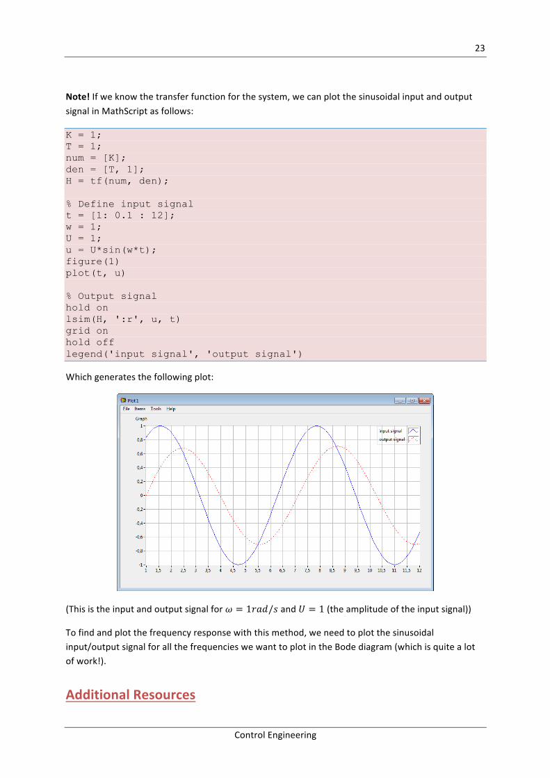
Note!Ifweknowthetransferfunctionforthesystem,wecanplotthesinusoidalinputandoutputsignalinMathScriptasfollows:
K = 1; T = 1; num = [K]; den = [T, 1]; H = tf(num, den); % Define input signal t = [1: 0.1 : 12]; w = 1; U = 1; u = U*sin(w*t); figure(1) plot(t, u) % Output signal hold on lsim(H, ':r', u, t) grid on hold off legend('input signal', 'output signal')
Whichgeneratesthefollowingplot:
(Thisistheinputandoutputsignalfor𝜔 = 1𝑟𝑎𝑑/𝑠and𝑈 = 1(theamplitudeoftheinputsignal))
Tofindandplotthefrequencyresponsewiththismethod,weneedtoplotthesinusoidalinput/outputsignalforallthefrequencieswewanttoplotintheBodediagram(whichisquitealotofwork!).
AdditionalResources

24
ControlEngineering
• http://home.hit.no/~hansha/?lab=mathscript
Here you will find tutorials, additional exercises, etc.