exercise 1. control in matlab€¦ · control in matlab this exercise is intended to give a basic...
TRANSCRIPT

Exercise 1. Control in Matlab
This exercise is intended to give a basic introduction to Matlab. The main focus will
be on the use of Control Systems Toolbox for control system analysis and design.
This toolbox will be used extensively during the upcoming exercises and laboratories
in the course. A short Matlab reference guide and a guide to the most commonly
used commands from Control Systems Toolbox can be found at the end of this
exercise.
Getting started
Matlab is started by issuing the command
> matlab
which will bring up a Java-based interface with three different frames showing the
current directory, your defined variables, and the Matlab command window. This
gives a good overview, but may be slow.
An alternative way to start Matlab is by the command
> matlab -nodesktop
which will only open up the command window. You can then use the commands ls
and whos to examine the current directory and your defined Matlab variables.
All Matlab commands have a help text, which is displayed by typing
>> help <command>
Try for example
>> help help
Use the help command frequently in the following exercises.
Matrices and system representations
Matrices in Matlab are created with the following syntax
>> A = [1 2;3 4]
A =
1 2
3 4
with semi-colons being used to separate the lines of the matrix. The transpose of amatrix is written as
>> A’
ans =
1 3
2 4
1

Exercise 1
1.1 Consider the following state-space model describing the dynamics of an
inverted pendulum
dx
dt=
0 1
1 0
x(t) +
1
0
u(t)
y(t) =
0 1
x(t)(1.1)
Enter the system matrices A, B, and C in Matlab and use the command
eig to determine the poles of the system.
In Control System Toolbox, the basic data structure is the linear time-invariant
(LTI) model. There is a number of ways to create, manipulate and analyze models(type, e.g., help ltimodels). Some operations are best done on the LTI system, andothers directly on the matrices of the model.
1.2 Define an LTI model of the pendulum system with the command ss. Use
the command tf to determine the transfer function of the system.
1.3 Zeros, poles and stationary gain of an LTI model is computed with the
command zpkdata. Use this command on the inverted pendulum model.
Compare with 1.1.
The command tf is used to create an LTI model from a transfer function. This isdone by specifying the coefficients of the numerator and denominator polynomials,e.g.
>> %% Continuous transfer function P(s) = 1 / (2s+1)
>> P = tf(1, [2 1]);
Another convenient way to create transfer function models is by the following com-mands
>> s = tf(’s’);
>> P = 1 / (2*s + 1);
To specify a time delay, set the property InputDelay of the LTI model
>> P.InputDelay = 0.5;
To display all properties of an LTI model and their respective values, type
>> get(P)
1.4 Define an LTI model of the continuous-time transfer function
P(s) = 1
s2 + 0.6s+ 1 ⋅ e−1.5s (1.2)
and use the commands step, nyquist, and bode to plot time- and frequency
responses of the system. Is the system stable? Will the closed-loop system
be stable if unit gain negative feedback is applied?
2

Exercise 1
State feedback example
Now return to the model of the inverted pendulum (1.1). We want to design astate-feedback controller
u(t) = −Lx(t)such that the closed loop system gets the characteristic equation
s2 + 1.4s+ 1 = 0
1.5 Is the system controllable? Use the command ctrb to compute the controlla-
bility matrix. Then use the command place to determine the state-feedback
vector L.
Connecting systems
LTI systems can be interconnected in a number of ways. For example, you may
add and multiply systems (or constants) to achieve parallel and series connections,respectively. Assume that the system (1.2) without time delay is controlled by a PDcontroller, C(s) = K (1+ sTd), with K = 0.5 and Td = 4, according to the standardblock diagram to the left in Figure 1.1:
yucl
uΣΣΣ
−1
+
–
P(s)C(s) SYS1
SYS2
Figure 1.1 A closed loop control system.
1.6 Define an LTI model of the controller, C(s). Compute the amplitude marginand phase margin for the loop transfer function. Use the Matlab command
margin.
There is a function feedback for constructing feedback systems. The block diagram
to the right in Figure 1.1 is obtained by the call feedback(SYS1,SYS2). Note the
sign conventions. To find the transfer function from the set point uc to the output
y, you identify that SYS1 is P(s)C(s) and SYS2 is 1.
1.7 Compute the transfer function for the closed-loop system, both using the
feedback command and by direct computation (use minreal to simplify)according to the formula
Gcl(s) =P(s)C(s)1+ P(s)C(s)
1.8 Plot the step response of the closed-loop system. What is the stationary gain
from uc to y?
3

Exercise 1
1.9 The systems you have seen so far have been SISO (Single-Input, Single-Output) systems. In this course we will also work with MIMO (Multiple-Input, Multiple-Output) systems. This problem gives you an example of aMIMO system.
A rough model for the pitch dynamics of a JAS 39 Gripen is given by
x =
−1 1 0 −1/2 0
4 −1 0 −25 8
0 1 0 0 0
0 0 0 −20 0
0 0 0 0 −20
x +
0 0
3/2 1/20 0
20 0
0 20
u
y=
0 1 0 0 0
0 0 1 0 0
x
(1.3)
Enter this system into Matlab using the ss command and determine if the
system is stable/controllable/observable? What is your conclusion from thisanalysis?
Can you find the transfer function from the second input (the elevator rud-der command) to the first output (the pitch rate)?
1.10 (*) In Matlab, a transfer function can be represented either on tf format,
corresponding to G1(s) and G3(s) below, or on zpk format, corresponding to
G2(s) and G4(s).Calculate the poles of the following systems
G1(s) =1
s3 + 3s2 + 3s+ 1
G2(s) =1
(s+ 1)3
During calculations, numerical round-off errors can arise, which can lead
to changed dynamics of the system. Calculate the poles of the following
systems where one coefficient has been modified.
G3(s) =1
s3 + 2.99s2 + 3s+ 1
G4(s) =1
(s+ 0.99)3
In view of your results on the poles of the four systems G1(s) to G4(s),discuss which format that is numerically the best.
1.11 (*) Consider the following state-space model of a system
dx
dt=
−1 0
0 −1
x(t) +
1
2
u(t)
y(t) =
3 4
x(t)(1.4)
Is the system observable? Is the system controllable? Motivate your answer
by calculations, but also with an insight how the system behaves.
4
Exercise 1
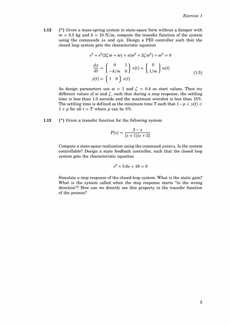
1.12 (*) Given a mass-spring system in state-space form without a damper withm = 0.5 kg and k = 10 N/m, compute the transfer function of the systemusing the commands ss and zpk. Design a PID controller such that the
closed loop system gets the characteristic equation
s3 + s2(2ζ ω +ω ) + s(ω 2 + 2ζ ω 2) +ω 3 = 0
dx
dt=
0 1
−k/m 0
x(t) +
0
1/m
u(t)
y(t) =
1 0
x(t)(1.5)
As design parameters use ω = 1 and ζ = 0.4 as start values. Then trydifferent values of ω and ζ , such that during a step response, the settlingtime is less than 1.0 seconds and the maximum overshot is less than 15%.
The settling time is defined as the minimum time T such that 1−p < y(t) <1+ p for all t > T where p can be 5%.
1.13 (*) Given a transfer function for the following system
P(s) = 3− s(s+ 1)(s+ 2)
Compute a state-space realization using the command ssdata. Is the system
controllable? Design a state feedback controller, such that the closed loop
system gets the characteristic equation
s2 + 5.6s+ 16 = 0
Simulate a step response of the closed-loop system. What is the static gain?
What is the system called when the step response starts “in the wrong
direction”? How can we directly see this property in the transfer function
of the process?
5

Exercise 1
Quick Matlab Reference
Some Basic Commands
Note: the command syntax is case-sensitive!
help <command> display the Matlab help for <command>.who lists all of the variables in your matlab workspace.
whos list the variables and describes their matrix size.
clear deletes all matrices from active workspace.
clear x deletes the matrix x from active workspace.
save saves all the matrices defined in the current session into
the file matlab.mat.
load loads contents of matlab.mat into current workspace.
save filename saves the contents of workspace into filename.mat
save filename x y z saves the matrices x, y and z into the file titled file-
name.mat.
load filename loads the contents of filename into current workspace; the
file can be a binary (.mat) file or an ASCII file.! the ! preceding any unix command causes the unix com-
mand to be executed from matlab.
Matrix commands
[ 1 2; 3 4] create the matrix
1 2
3 4
.
zeros(n) creates an nxn matrix whose elements are zero.
zeros(m,n) creates a m-row, n-column matrix of zeros.
ones(n) creates a n x n square matrix whose elements are 1’s
ones(m,n) creates a mxn matrix whose elements are 1’s.
ones(A) creates an m x n matrix of 1’s, where m and n are based on the
size of an existing matrix, A.
zeros(A) creates an mxn matrix of 0’s, where m and n are based on the
size of the existing matrix, A.
eye(n) creates the nxn identity matrix with 1’s on the diagonal.
A’ (complex conjugate) transpose of Adiag(V) creates a matrix with the elements of V on the diagonal.
blkdiag(A,B,C) creates block matrix with the matrices A, B, and C on the di-
agonal
6

Exercise 1
Plotting commands
plot(x,y) creates an Cartesian plot of the vectors x & y.
stairs(x,y) creates a stairstep of the vectors x & y.
semilogx(x,y) plots log(x) vs y.semilogy(x,y) plots x vs log(y)loglog(x,y) plots log(x) vs log(y).grid creates a grid on the graphics plot.
title(’text’) places a title at top of graphics plot.
xlabel(’text’) writes ’text’ beneath the x-axis of a plot.
ylabel(’text’) writes ’text’ beside the y-axis of a plot.
gtext(’text’) writes text according to placement of mouse
hold on maintains the current plot in the graphics window while
executing subsequent plotting commands.
hold off turns off the ’hold on’ option.
print filename -dps writes the contents of current graphics to ’filename’ in
postscript format.
Misc. commands
length(x) returns the number elements in a vector.
size(x) returns the size m(rows) and n(columns) of matrix x.rand returns a random number between 0 and 1.
randn returns a random number selected from a normal
distribution with a mean of 0 and variance of 1.
rand(A) returns a matrix of size A of random numbers.
fliplr(x) reverses the order of a vector. If x is a matrix,
this reverse the order of the columns in the matrix.
flipud(x) reverses the order of a matrix in the sense of
exchanging or reversing the order of the matrix
rows. This will not reverse a row vector!
reshape(A,m,n) reshapes the matrix A into an mxn matrix
from element (1,1) working column-wise.squeeze(A) remove empty dimensions from A
A.x access element x in the struct A
7

Exercise 1
Some useful functions from Control Systems Toolbox
Do help <function> to find possible input and output arguments.Creation and conversion of continuous or discrete time LTI models.
ss - Create/convert to a state-space model.
tf - Create/convert to a transfer function model.
zpk - Create/convert to a zero/pole/gain model.
ltiprops - Detailed help for available LTI properties.
ssdata etc. - Extract data from a LTI model.
set - Set/modify properties of LTI models.
get - Access values of LTI model properties.
minreal - Minimal realization and pole/zero cancellation.
Sampling of systems.
c2d - Continuous to discrete conversion.
d2c - Discrete to continuous conversion.
Model dynamics.
pole, eig - System poles.
zero - System zeros.
pzmap - Pole-zero map.
covar - Covariance of response to white noise.
State-space models.
ss2ss - State coordinate transformation.
canon - State-space canonical forms.
ctrb, obsv - Controllability and observability matrices.
Time response.
step - Step response.
impulse - Impulse response.
initial - Response of state-space system with given initial state.
lsim - Response to arbitrary inputs.
ltiview - Response analysis GUI.
Frequency response.
bode - Bode plot of the frequency response.
margin - Bode plot with phase and gain margins.
sigma - Singular value plot.
nyquist - Nyquist plot.
nichols - Nichols plot.
ltiview - Response analysis GUI.
ctrlpref - Open GUI for setting Control System Toolbox Preferences.
System interconnections.
+ and - - Add and subtract systems (parallel connection).
* - Multiplication of systems (series connection).
/ and \ - Division of systems (right and left, respectively).
inv - Inverse of a system.
[ ] - Horizontal/vertical concatenation of systems.
feedback - Feedback connection of two systems.
Classical design tools.
rlocus - Root locus.
place, acker - Pole placement (state feedback or estimator).
estim - Form estimator given estimator gain.
reg - Form regulator given state-feedback and estimator gains.
LQG design tools.
lqr,dlqr - Linear-quadratic (LQ) state-feedback regulator.
lqry - LQ regulator with output weighting.
lqrd - Discrete LQ regulator for continuous plant.
kalman, kalmd - Kalman estimator.
lqgreg - Form LQG regulator given LQ gain and Kalman estimator.
Matrix equation solvers.
dlyap - Solve discrete Lyapunov equations.
dare - Solve discrete algebraic Riccati equations.
8
Exercise 2. System Representations and
Stability
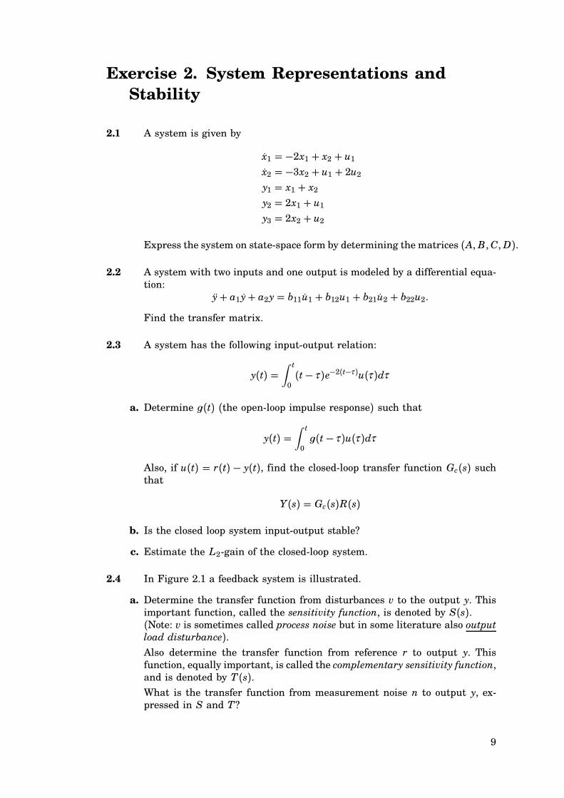
2.1 A system is given by
x1 = −2x1 + x2 + u1x2 = −3x2 + u1 + 2u2y1 = x1 + x2y2 = 2x1 + u1y3 = 2x2 + u2
Express the system on state-space form by determining the matrices (A, B,C,D).
2.2 A system with two inputs and one output is modeled by a differential equa-
tion:
y+ a1 y+ a2y = b11u1 + b12u1 + b21u2 + b22u2.
Find the transfer matrix.
2.3 A system has the following input-output relation:
y(t) =∫ t
0
(t− τ )e−2(t−τ )u(τ )dτ
a. Determine �(t) (the open-loop impulse response) such that
y(t) =∫ t
0
�(t− τ )u(τ )dτ
Also, if u(t) = r(t) − y(t), find the closed-loop transfer function Gc(s) suchthat
Y(s) = Gc(s)R(s)
b. Is the closed loop system input-output stable?
c. Estimate the L2-gain of the closed-loop system.
2.4 In Figure 2.1 a feedback system is illustrated.
a. Determine the transfer function from disturbances v to the output y. This
important function, called the sensitivity function, is denoted by S(s).(Note: v is sometimes called process noise but in some literature also outputload disturbance).Also determine the transfer function from reference r to output y. This
function, equally important, is called the complementary sensitivity function,
and is denoted by T(s).What is the transfer function from measurement noise n to output y, ex-
pressed in S and T?
9

Exercise 2
1.4s+ 1s
1
(s+ 1)2+
+
++
−1
r y
v
n
d
C(s) P(s)
Figure 2.1 System in Problem 2.4
10−1
100
101
10−2
10−1
100
101
10−1
100
101
10−2
10−1
100
101
Magnitude(abs)
Magnitude(abs)
Frequency (rad/sec)Figure 2.2
b. Figure 2.2 shows gain curves for the sensitivity function and the comple-
mentary sensitivity function. Which curve represents which function?
c. In which frequency region (roughly) is there good tracking of the referencevalue?
d. In which frequency region (roughly) is there good attenuation of the mea-surement noise, n?
2.5 Study the feedback control system in Figure 6.5, where the process, P(s),is given by
P(s) = 1
(s+ 1)(s + 2)
The Bode diagram of P(s) is shown in Figure 2.4.
Three different controllers were designed
C1(s) = 10 C2(s) = 10s+ 1s
C3(s) = 10s+ 1se−0.1s
where the last one has a small delay.
10

Exercise 2
C(s) P(s)+
+
++
−1
r y
v
n
d
Figure 2.3 System in Problem 2.5
10−4
10−3
10−2
10−1
100
Ma
gn
itu
de
(a
bs)
10−2
10−1
100
101
102
−180
−135
−90
−45
0
Ph
ase
(d
eg
)
Bode Diagram
Frequency (rad/sec)
Figure 2.4 Bode diagram for P(s) in Problem 2.5.
a. Figure 2.5 shows sensitivity functions, corresponding to the three different
control designs C1−C3. Combine the controllers C1−C3 with the sensitivityfunctions A− C. Motivate!
b. Figure 2.6 shows responses to a step load disturbance, d, corresponding to
the three different control designs C1− C3. Combine the controllers C1− C3with the load step responses I − I I I. Motivate!
2.6 Consider a water tank with a separating wall. The wall has a hole at the
bottom, as can be seen in figure 2.7.
The input signals are the inflows of water to the left, u1, and the right, u2,
halves of the tank, measured in cm3/s. The water levels are denoted by h1cm and h2 cm, respectively. The outflow y cm
3/s is considered proportionalto the water level in the right half of the tank:
y(t) = α h2(t)
11

Exercise 2
10−1
100
101
102
10−1
100
101
A
10−1
100
101
102
B
10−1
100
101
102
C
Bode Diagram
Frequency (rad/sec)
Magnitude (
abs)
Figure 2.5 Sensitivity functions for Problem 2.5.
0 5 10−0.8
−0.6
−0.4
−0.2
0
0.2
0.4
0.6
0.8
1
1.2
I
0 5 10
II
0 5 10
III
Step Response
Time (sec)
Ou
tpu
t
Figure 2.6 Step Load Disturbance Responses for Problem 2.5.
The flow between the tank halves is proportional to the difference in level:
f (t) = β (h1(t) − h2(t))
(flow from left to right)The signals hi,ui and y are thought of as deviations from a linearization
point, and may therefore be negative. Assume that the two tank halves each
have area A1 = A2 = 1 cm2.
a. Write the system on state-space form.
b. What is the transfer matrix from (u1 u2 )T to y?
c. What is the L2-gain of the system when α = β = 1? (Hint: Use Matlab.)
d. It turns out that the L2-gain is larger than one. How is this possible? Can
there be more water coming out from the tank than what is poured into it?
Have we invented a water-producing device? Explain what’s wrong here!
12

Exercise 2
Figure 2.7
2.7 (*) A PI controller
U(s) =(
1+ 1s
)(R(s) − Y(s)
)
is used to control a servo process, which is modeled as
Y(s) = 1
ms2 + 2sU(s) m > 0
This problem is about investigating for what values of the mass m the
closed loop system is stable, using the Nyquist criterion. Before we can do
that however, we need to write the system in another form.
a. Find the characteristic polynomial of the closed-loop system. Show that the
same characteristic polynomial can be generated by a feedback loop between
some systemQ(s)P(s) and d where m = d + 1. See figure 2.8. Determine Q(s)
and P(s) so that they are not dependent on d.
Q(s)P(s)r yd
−1
+
Figure 2.8 Closed-loop system for Problem 2.7.
b. Use the Nyquist criterion onQ(s)P(s) to determine the values of d (and hence
m) for which the closed-loop system is stable. Use Matlab.
c. Let m = 1, but suppose there is a time delay τ in the measurement so thatU(s) = (1+ 1/s)e−sτ
(R(s) − Y(s)
). How large time delays can be tolerated
before the system becomes unstable?
13

Exercise 2
d. Suppose that the servo instead has some unmodeled dynamics ∆(s)
Y(s) =(
1
s2 + 2s(1+ s∆(s)))
U(s)
Rewrite the closed-loop system as a feedback loop between ∆(s) and a trans-fer function H(s). Determine a number γ such that the small gain theoremguarantees stability for all ∆(s) with q∆q∞ < γ .
14

Exercise 3. Disturbance Models and
Robustness
3.1 a. Analyze the stability of the system to the left in Figure 3.1 using the small
gain theorem.
b. Analyze how the stability of the system to the right in Figure 3.1 depends
on the feedback gain K . If you get different results from a, explain why!
a)
Σ 1s+1
∆b)
Σ 1s+1
−K
Figure 3.1
3.2 Consider the system in Figure 3.2.
2s+ 2s
1
(s+ 1)2
v∆n
+
s
s+ 2
−1
P(s)C(s)
Figure 3.2 System for Problem 3.2.
a. Find the transfer function Gvn from n to v.
b. How large is the gain qGvnq∞? Support the solution by a Matlab plot.
c. Using the small gain theorem, find the largest possible L2-gain of ∆ forwhich the closed loop system is stable.
d. The ∆ block is used to account for uncertainty in the process model. Explainthe role of the factor s
s+2 multiplying ∆.
3.3 A feedback system is shown in Figure 3.3.
a. Compute the poles of the closed loop system. You may use Matlab.
15

Exercise 3
0.81s+ 3.60.225s
1
(s+ 2)+
+
++
−1
r y
v
n
d
C(s) P(s)
Figure 3.3 System in Problem 3.3.
b. Derive the transfer functions from r,d,v and n to y. Identify the sensitivity
function S and the complementary sensitivity function T . Plot them in the
same Bode plot.
c. If we have a disturbance v = sin(0.5t) acting on the system and all otherinput signals are zero, what amplitude would the oscillations in the output
signal have when the transients have disappeared?
d. If we have sinusoidal measurement disturbances n(t) with a frequency of 50Hz and unit amplitude and all other input signals are zero, what amplitude
would the oscillations in the output signal have when the transients have
disappeared?
3.4 (*) Consider the system in Figure 3.4.
0.81s+ 3.60.225s
1
(s+ 2)
v∆n
+
s
s+ 1
−1
P(s)C(s)
Figure 3.4 System for Problem 3.4.
a. What is the largest possible bound on the L2-gain of ∆, for which the closedloop system is stable, by the small gain theorem? Support the solution by
a Matlab plot.
b. If ∆(s) is replaced by a real parameter δ , then for what values of δ is theclosed loop stable? Compare with the gain bound in (a).
c. What is the difference between the uncertainty model in this problem and
the one in problem 3.2?
16

Exercise 3
3.5 A continuous-time stochastic process u(t) has the power spectrum Φu(ω ).The process can be represented by a linear filter that has white noise as
input. Determine the linear filter when
a.
Φu(ω ) =a2
ω 2 + a2
b.
Φu(ω ) =a2b2
(ω 2 + a2)(ω 2 + b2)
3.6 Consider a missile travelling in the air. It is propelled forward by a jet
force u along a horizontal path. The coordinate along the path is z. We
assume that there is no gravitational force. The aerodynamic friction force
is described by a simple model as
f = k1 ⋅ z+ v,
where v are random variations due to wind and pressure changes. Combin-
ing this with Newton’s second law, mz = u− f , where m is the mass of themissile, gives the input-output relation
z+ k1mz = 1m(u− v).
a. Express the input-output relation in state-space form.
b. The disturbance v has been determined to have the spectral density
Φv(ω ) = k0 ⋅1
ω 2 + a2
Expand your state-space description so that the disturbance input can be
expressed as white noise. What is the new input-output relation?
3.7 (*) This problem builds on problem 3.6.
a. Assume that the position measurement is distorted by an additive error
n(t),y(t) = z(t) + n(t)
Write down the state-space equations for the system, assuming that n(t) iswhite noise with intensity 0.1, i.e. Φn(ω ) " 0.1.
b. Solve the same problem, this time with
Φn(ω ) = 0.1ω 2
ω 2 + b2 .
c. Solve the problem with
Φn(ω ) = 0.11
ω 2 + b2 .
17

Exercise 3
3.8 (*) A system is given by
x = Ax + Bu+ Nwy = Cx + n
The load disturbance w is piecewise constant, that is, it changes in steps.
The measurement noise n is periodic with a frequency of 2 Hz.
Expand the system model to include the known characteristics of the dis-
turbances.
3.9 (*) Consider a swing (swe: gunga) that is hanging outside in the wind. Theswing is described by the transfer function
Y(s) = 1
s2 + s+ 1U(s)
where the output signal y(t) is the angle of the swing (relative to the verticalaxis) and the input signal u(t) is the moment around the pivotal point. Theinfluence of wind can be described as
u(t) = Kv(t)
where v(t) is a normally distributed disturbance with spectrum
Φv(ω ) =2α
α 2 +ω 2, α > 0.
K is a measure of the wind strength and α is a measure of the occurrenceof wind gusts (swe: vindbyar).
a. Does α increase or decrease when there are more wind gusts (i.e., whenthe wind changes strength and direction more often)?
b. Determine the variance of y(t). What is your interpretation?Hint:
1
2π
∫ ∞
−∞
pb2(iω )2 + b1iω + b0p2p(iω )3 + a2(iω )2 + a1iω + a0p2
dω
= b22a0a1 + (b21 − 2b0b2)a0 + b20a2
2a0(−a0 + a1a2)
3.10 (*) Consider an electric motor with the transfer function
G(s) = 1
s(s+ 1)
from input current to output angle.
There are two different disturbance scenarios:
(i) y(t) = G(p)(u(t) +w(t))(ii) y(t) = G(p)u(t) +w(t)
18

Exercise 3
In both cases, w(t) = v(t), where v(t) is a unit disturbance, e.g. an impulse.
a. Draw a block diagram of the two cases.
b. Put both cases in state-space form. It is assumed in the second case that
the disturbance does not give cause to any common states with the engine.
c. Give a physical interpretation of w(t) is, in the two cases.
19

Exercise 4. Loop Shaping
Exercises 4.1–4.4 are preparatory exercises for laboratory exercise 1. In these exer-
cises, we will design a controller, step by step, for the process given by the transfer
function
P(s) = 1
s2 + 0.7s+ 1
4.1 Create a transfer function object in Matlab, and take a look at the Bode and
Nyquist diagrams of the process. In the following exercises you will use a
number of different controllers to shape the Bode diagram of the open loop
system.
The structure of the control system is given in Figure 4.1. As you may have
already heard, several transfer functions should be studied in a design.
Besides a nice step response from r to y, also a fast recovery from, e.g., load
disturbances, d is required. Furthermore, it is important to see how the
control signal responds to the different input signals.
+ ++
−1
F(s) C(s) P(s)
d n
r yu
Figure 4.1 Our control loop with reference signal r, load disturbance d, measurement noise
n and output y.
We have two degrees of freedom in designing our controller; the feedback
part C(s) and the prefilter F(s).We start by designing C(s). For evaluation, we can look at the effect of astep load disturbance d (as this is only affected by the feedback loop). A goodload step disturbance response goes quickly to zero. What is the closed-loop
transfer function from d to y?
a. We will first try to control the system using a simple P-controller. Simulate
load step responses for K=0.1, 1.0, 5.0, 10.0. Does the output go to zero?How much stationary error is left for different K ’s?
Tip: Use the Matlab command figure(n) to draw several plots. E.g:
>> figure(1)
>> bode(P*C, P) % Plot both the process and the
>> % compensated open loop process
>> figure(2)
>> step(P/(1+C*P)) % Plot step load disturbance
>> figure(3)
>> bode(P/(1+C*P)) % Bode-plot of closed loop from
>> % load disturbance
20
Exercise 4
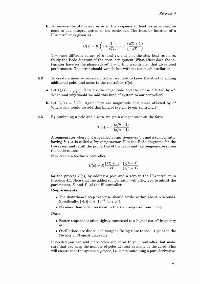
b. To remove the stationary error in the response to load disturbances, we
need to add integral action to the controller. The transfer function of a
PI-controller is given as
C(s) = K(
1+ 1
sTi
)
= K(sTi + 1sTi
)
Try some different values of K and Ti, and plot the step load response.
Study the Bode diagram of the open-loop system. What effect does the in-
tegrator have on the phase curve? Try to find a controller that gives good
performance. The error should vanish fast without too much oscillation.
4.2 To create a more advanced controller, we need to know the effect of adding
additional poles and zeros to the controller, C(s).
a. Let Ca(s) = 1s/a+1 . How are the magnitude and the phase affected by a?.
When and why would we add this kind of system to our controller?
b. Let Cb(s) = s/b+11. Again, how are magnitude and phase affected by b?
When/why would we add this kind of system to our controller?
4.3 By combining a pole and a zero, we get a compensator on the form
C(s) = K (s/b+ 1)(s/a+ 1)
A compensator where b < a is called a lead-compensator, and a compensatorhaving b > a is called a lag-compensator. Plot the Bode diagrams for thetwo cases, and recall the properties of the lead- and lag-compensators from
the basic course.
Now create a feedback controller
C(s) = K (sTi + 1)sTi
⋅(s/b+ 1)(s/a+ 1)
for the process P(s), by adding a pole and a zero to the PI-controller inProblem 4.1. Note that the added compensator will allow you to adjust the
parameters, K and Ti, of the PI-controller.
Requirements:
• The disturbance step response should settle within about 5 seconds.Specifically, py(t)p < 4 ⋅ 10−3 for t > 5.
• No more than 20% overshoot in the step response from r to y.
Hints:
• Faster response is often tightly connected to a higher cut-off frequencyω c.
• Oscillations are due to bad margins (being close to the −1 point in theNichols or Nyquist diagrams).
If needed you can add more poles and zeros to your controller, but make
sure that you keep the number of poles at least as many as the zeros. This
will ensure that the system is proper, i.e. is not containing a pure derivative.
21

Exercise 4
4.4
a. Calculate the closed-loop transfer function Gyr(s) from reference r to out-put y with your controller in the loop. What would be the ideal frequency
response for this transfer function?
b. The control signal u(t) to the process is physically limited by
−10 ≤ u(t) ≤ 10,
which must be taken into account in the design. This limits how fast we
can change the process.
Simulate the step response. Is the constraint on u(t) satisfied? ImproveGyr(s) by tuning the prefilter F(s) so that the step response behaves nicely.How should F(s) compensate Gyr(s) in the frequency domain?
4.5 (*) A servo system has the transfer function:
Go(s) =2.0
s(s+ 0.5)(s+ 3)
The closed system has a step response according to Figure 4.2. It is clear
that the system is poorly damped and has a large overshoot. It is, however,
fast enough. Create a lead controller that stabilizes the system by increasing
the phase margin to φm = 50○, without changing the cut-off frequency.(φm = 50○ gives a relative damping of ζ ( 0.5 which achieves an overshootof M ( 17%). The stationary error for the closed system is 0.75 for a ramp-shaped input signal. The error for a ramp function at the compensated
system must not exceed 1.5.
0 5 10 15 20 25 30 35 40 450
0.2
0.4
0.6
0.8
1
1.2
1.4
1.6
Step Response
Time (sec)
Am
plit
ud
e
Figure 4.2 Step response from the closed servo system in 4.5.
4.6 (*) Consider the control system in Figure 4.1, where the plant is describedby
P(s) = 1
(s+ 1)(s+ 0.02)
22

Exercise 4
and F(s) = 1. A non-control experienced engineer has designed the con-troller
C(s) = (s+ r)s
with r = 0.02, but the resulting control system reacts extremely slowly tostep disturbances in d. The reason is that the slow pole in −0.02 is canceledby the controller zero.
The Bode diagrams of the plant, the controller, and the open-loop system
are shown in Figure 4.3.
10−3
10−2
10−1
100
101
10−2
100
102
104
Bode diagramM
ag
nitu
de
P(s)C(s)P(s)C(s)
10−3
10−2
10−1
100
101
−200
−150
−100
−50
0
Frequency [rad/s]
Ph
ase
[d
eg
]
Figure 4.3 The Bode diagrams of P(s), C(s) and the open loop P(s)C(s) when r = 0.02.
a. The load disturbance d is typically most significant at low frequencies, so
we are interested in keeping the magnitude of the transfer function Gydfrom d to y significantly smaller than 1 in a frequency range [0,ω b]. Whatis (approximately) ω b if you use the given controller? Use the Bode diagramin Figure 4.3.
b. To reject the disturbance d faster,ω b should be increased. For noise reasons,we want the cross-over frequency of the system to be the same.
How should the value of r in the controller be changed to achieve this?
Motivate your design by showing that:
• The range [0,ω b] where you get good disturbance rejection of d is in-creased.
• The cross-over frequency of the system is still approximately the same.
Exact proofs are not required; some Bode-diagram reasoning will do.
23

Exercise 5. Multivariable Zeros, Singular
Values and Controllability/Observability
5.1 Consider the following system
x =
−1 0 0
0 −2 0
0 0 −3
x +
1
1
0
u
y =
1 0 1
x
a. Show that the system is neither controllable nor observable. Also determine
the uncontrollable and unobservable modes.
b. Determine the transfer function of the system and the order of a minimal
state space realisation. How can this be related to the controllable and
observable states of the system?
5.2 The following model of a heat exchanger was presented in the course book
(see Example 2.2)
x =
−0.21 0.2
0.2 −0.21
x +
0.01 0
0 0.01
u
y=
1 0
0 1
x,
where the first state represents the temperature of the cold water and the
second state is the temperature of the warm water.
a. Use Matlab to calculate the controllability Gramian.
b. What state direction is hardest to control?
5.3 (*) In the first exercise session we were given a rough model of the pitchdynamics of JAS 39 Gripen
x =
−1 1 0 −1/2 0
4 −1 0 −25 8
0 1 0 0 0
0 0 0 −20 0
0 0 0 0 −20
x +
0 0
3/2 1/20 0
20 0
0 20
u. (5.1)
Using Matlab:
a. Show that there is no scalar output signal that makes the system observ-
able.
Hint: Use symbolic toolbox to determine a general C matrix and calculate
the observability matrix. For instance, the following lines of Matlab code
may help you:
24

Exercise 5
>> syms c1 c2 c3 c4 c5
>> C = [c1 c2 c3 c4 c5]
>> Wo = ...
b. Let the output be
y(t) =
1 0 0 0 0
0 1 0 0 0
x(t).
Which are the non-observable modes?
5.4 In Figure 5.1 and Figure 5.2 you see an interconnection of two systems P1 =s+ 3s+ 2 and P2 =
s+ 1(s+ 3)(s+ 4)(s− 2) . One can notice that after multiplying
the two systems we can cancel a pole and a zero in s0 = −3. Usually itmeans that the whole system is not observable, or not controllable. Which
of these two situations are depicted in the Figure 5.1 and Figure 5.2?
P1 P2
Figure 5.1 Block diagram for problem 5.4.
P2 P1
Figure 5.2 Block diagram for problem 5.4.
5.5 Consider the following transfer function matrix
G(s) =
1
s+ 2 − 1
s+ 21
s+ 2s+ 1s+ 2
a. Determine the pole and zero polynomials for this system. What is the least
order needed to realize the system on state space form?
b. Find a state-space realization of the system.
c. Use Matlab to draw a singular value plot for the system. What is theL2-gain
of the system?
5.6 Consider the system
G(s) =
1 1/s
with two inputs and one output.
a. Use Matlab to determine the singular values of the system at ω = 1 rad/s,together with the input directions giving the maximum and minimum out-
put gains respectively.
25

Exercise 5
b. The derived input directions are complex. What does this mean? Explain
why it’s logical that these received input directions are those giving the
smallest and highest system gains respectively for this particular system.
5.7 The following is an idealized dynamic model of a distillation column:
G(s) = 1
75s+ 1
87.8 −86.4108.2 −109.6
a. Using Matlab, plot the singular values of the process.
b. For the frequencies ω = 0, 0.1 rad/s, calculate the gains of the systemin the input directions d1 = [0.6713 0.7412]T and d2 = [1 0]T , i.e. theamplification of the input di ⋅ sin(ω ) by the transfer matrix G(s).
c. Determine the minimum and maximum output gains respectively at ω = 0rad/s as well as the input directions associated with them. Will the direc-tions depend on frequency for this particular system? Explain your answer.
26

Exercise 6. Fundamental Limitations
6.1 Consider the ball in the hoop in Figure 6.1. This process consists of a cylin-
der rotating with the angular velocityω . Inside the cylinder, a ball is rolling.The position of the ball is given by the angle θ and the linearized dynamicscan be written as θ + cθ + kθ = ω . Let k = 1 and c = 2.
a. What is the transfer function from cylinder velocity ω to the position θ ofthe ball? Where is the zero located?
b. What limitation on the sensitivity function for a stable closed loop system
is imposed by the process zero?
c. What consequence does the process zero have on the static error when a
reference signal r(t), e.g. a step with the magnitude a, is to be followed. Letthe control signal ω (t) be determined from the error signal r(t) − θ (t) viathe controller transfer function C(s). Give a physical interpretation.
d. Usually a controller integrator is introduced in order to remove static errors.
How would the ball/hoop-system behave with a PI controller and a non-zeroreference position for the ball?
ω
θ
Figure 6.1 The ball in the hoop.
6.2 A resonant mechanical system has the pole-zero configuration shown in
Figure 6.2. The controller structure is given by Figure 6.3.
a. What constraint does a purely imaginary process pole in iω p impose on theBode diagram of the sensitivity function?
b. What consequence does this give for the control error e, in presence of a
sinusoidal measurement disturbance n with frequency ω p?
c. What effect does the controller C(s) have on this response?
d. What constraint does a purely imaginary process zero in iω z impose on thesensitivity function?
e. What consequence does this give for the response x, in presence of a sinu-
soidal measurement disturbance n with a frequency ω z?
27

Exercise 6
−15 −10 −5 0 5
x 104
−3
−2
−1
0
1
2
3x 10
4
Figure 6.2 Pole-zero configuration of a resonant mechanical system.
F C P
−1
ΣΣΣr e u
d
x
n
y
Figure 6.3 Two degree of freedom controller structure.
6.3 Consider the setup in Figure 6.3 with P(s) = (3− s)/(s+ 1)2
a. Does there exist a stabilizing controller C(s) such that the transfer functionfrom n to x becomes 5/(s+ 5) ? (Note: All transfer functions in the gang offour must be stable.)
b. Show that the specification
pS(iω )p ≤ 2ω√ω 2 + 36
ω ∈ IR
is equivalent to
supωpWa(iω )S(iω )p ≤ 1
with a = 6 andWa(s) =
s+ a2s
Is this specification possible to satisfy ?
c. Use Matlab to find a stabilizing controller C(s) such that∣∣∣∣
1
1+ PC (iω )∣∣∣∣≤ 2ω√
ω 2 + 1for ω ∈ [0, 2]
Hint: Use a PI controller on the form:
C(s) = K s/b+ 1s
28

Exercise 6
10−2
10−1
100
101
102
10−2
10−1
100
101
Figure 6.4 Gain specification for the closed-loop transfer function T in problem 6.4.
6.4 For each of the following three design problems, state if it is possible to con-
struct a controller that can achieve the given specification. Motivate your
answers! (Hint: It is not possible in at least two of the cases.)System: Specification:
P1(s) =e−2s
s+ 2The step response must reach 0.9 before t = 1.
P2(s) = 3(s+ 40)(s − 20)s2(s− 10)
The gain curve of the closed-loop transfer func-
tion T should lie between the two gain curves
depicted in Figure 6.4.
P3(s) =1
s− 3The step response must stay in the interval [0, 2]for all t.
6.5 (*) The specifications
supωpWS(iω )S(iω )p ≤ 1 sup
ωpWT(iω )T(iω )p ≤ 1
can be used to make sure that the sensitivity is small in a low frequency
range and measurement noise is rejected in a high frequency range.
a. Show that the two specifications are incompatible if
pWS(s)p = pWT(s)p > 2
for some right half plane s. (Hint: Use that S+ T = 1.)
b. Show that the two specifications are incompatible if
WS(s) =(s+ 0.1s
)n
WT(s) =(s+ 1010
)n
and n ≥ 8.Hint: Use the result of a.
29

Exercise 6
C(s) P(s)+
+
++
−1
r y
v
n
d
Figure 6.5 System in Problem 6.6
6.6 A multi-variable system (block diagram in Figure 6.5) is supposed to atten-uate all output load disturbances (v) with at least a factor 10 for frequenciesbelow 0.1 rad/sec. Constant output load disturbances should be attenuatedby at least a factor 100 in stationarity.
Furthermore, the system should also attenuate measurement disturbances
(n) with at least a factor 10 for frequencies above 2 rad/sec.
a. Formulate specifications on (the singular values of) S and T that guaranteethe above requirements.
b. Re-formulate the specifications in a using q ⋅q∞ and the weighting functionsWS and WT .
c. (*) Give conditions on the open-loop gain pL(iω )p = pP(iω )C(iω )p that aresufficient to fulfill these specifications.
d. (*) What cut-off frequency and what phase margin could have been ex-pected, following your answer in c, if the system had been SISO? What
lower bound on qTq∞ does this give?
6.7 Consider the setup in Figure 6.3 with
P(s) = 6− ss2 + 5s+ 6
Give an upper bound for how fast the closed loop system can be made. That
is, give a value a such that the following specification is impossible to satisfy
if c > a.
pS(iω )p ≤ 2ω√ω 2 + c2
ω ∈ IR
30

Exercise 7. Controller Structures and
Preparations for Laboratory Exercise 2
Note: Exercises 7.1-7.3 serve as preparation for Laboratory Excercise 2.
7.1 a. Give the definition of RGA for a complex valued, not necessarily square,
matrix A. How do you apply it to a process G(s) and what information canbe extracted in an automatic control perspective?
b. Let
G(s) =( 1s+2
10s+1
1s+5
5s+3
)
.
Compute RGA(G(0)).
c. What input-output pairing would you recommend be used in a decentralised
control structure?
7.2 Consider the MIMO process
P(s) =
1
s+ 1 0 0
00.1
s+ 101
s+ 100.1
s+ 11
s+ 1 0
.
Compute the relative gain array, RGA, of P(0) and suggest an input-outputpairing for the system based on this.
Hint: The inverse of P(s) is given by
P(s)−1 =
s+ 1 0 0
−0.1(s+ 1) 0 s+ 10.01(s+ 1) s+ 10 −0.1(s+ 1)
.
7.3 Figure 7.1 shows the quadruple-tank process that will be used in Lab 2.
The goal is to control the levels in the lower tanks (y1, y2) using the pumps(u1, u2). For each tank i = 1 . . . 4, mass balance and Bernoulli’s law givethat
Aidhi
dt= −ai
√
2�hi + qin (7.1)
where Ai is the cross-section of the tank, hi is the water level, ai is the
cross-section of the outlet hole, � is the acceleration of gravity, and qinis the inflow to the tank. The non-linear equation (7.1) can be linearizedaround a stationary point (h0i , q0in), giving the linear equation
Aid∆hidt
= −ai√
�2h0i
∆hi + ∆qin (7.2)
31

Exercise 7
u1 u2
y1 y2Tank 1 Tank 2
Tank 3 Tank 4
Pump 1 Pump 2
Figure 7.1 The quadruple-tank process.
where ∆hi = hi − h0i , and ∆qin = qin − q0in denote deviations around thestationary point.
The flows from the pumps are divided according to two parameters γ 1,γ 2 ∈(0, 1). The flow to Tank 1 is γ 1k1u1 and the flow to Tank 4 is (1− γ 1)k1u1.Symmetrically, the flow to Tank 2 is γ 2k2u2 and the flow to Tank 3 is(1− γ 2)k2u2.
a. Let ∆ui = ui−u0i , ∆hi = hi−h0i , and ∆yi = yi− y0i . Verify that the linearizeddynamics of the complete quadruple-tank system are given by
d∆h1dt
= − a1A1
√ �2h01
∆h1 +a3
A1
√
�2h03
∆h3 +γ 1k1A1
∆u1
d∆h2dt
= − a2A2
√ �2h02
∆h2 +a4
A2
√ �2h04
∆h4 +γ 2k2A2
∆u2
d∆h3dt
= − a3A3
√
�2h03
∆h3 +(1− γ 2)k2A3
∆u2
d∆h4dt
= − a4A4
√ �2h04
∆h4 +(1− γ 1)k1A4
∆u1
Introduce the input vector, u, output vector, y, and state vector, x, as
u =
∆u1
∆u2
, x =
∆h1
∆h2
∆h3
∆h4
, y =
∆y1
∆y2
.
32

Exercise 7
Verify that the linearized system can be written on state-space form as
dx
dt=
− 1T1
0A3
A1T30
0 − 1T2
0A4
A2T4
0 0 − 1T3
0
0 0 0 − 1T4
x +
γ 1k1A1
0
0γ 2k2A2
0(1− γ 2)k2A3
(1− γ 1)k1A4
0
u,
y=
kc 0 0 0
0 kc 0 0
x,
where Ti =Ai
ai
√
2h0i� , and kc is a measurement constant.
b. Show that the transfer matrix from u to y is given by
P(s) =
γ 1c11+ sT1
k2
k1⋅
(1− γ 2)c1(1+ sT1)(1+ sT3)
k1
k2⋅
(1− γ 1)c2(1+ sT2)(1+ sT4)
γ 2c21+ sT2
where c1 = T1k1kc/A1 and c2 = T2k2kc/A2.Hint: Use the fact that
a 0 b 0
0 c 0 d
0 0 e 0
0 0 0 f
−1
=
1
a0 − b
ae0
01
c0 − d
c f
0 01
e0
0 0 01
f
c. The zeros are given by the equation
det P(s) = c1c2(γ 1γ 2(1+ sT3)(1+ sT4) − (1− γ 1)(1− γ 2)
)
(1+ sT1)(1+ sT2)(1 + sT3)(1+ sT4)= 0
which is simplified to
(1+ sT3)(1+ sT4) −(1− γ 1)(1− γ 2)
γ 1γ 2= 0.
Show that the system is minimum phase (i.e., that both zeros are stable)if 1 < γ 1 + γ 2 < 2, and that the system is non-minimum phase (i.e., that atleast one zero is unstable) if 0 < γ 1 + γ 2 < 1.Hint: A second-order polynomial has all of its roots in the left half plane if
and only if all coefficients have the same sign.
In the lab, we will first study the case γ 1 = γ 2 ( 0.7, and then the caseγ 1 = γ 2 ( 0.3. In which case will the process be more difficult to control?
33

Exercise 7
d. Show that the RGA for P(0) is given by
λ 1− λ
1− λ λ
where λ = γ 1γ 2/(γ 1 + γ 2 − 1).Based on this RGA matrix, suggest an input-output pairing in the two cases
γ 1 = γ 2 ( 0.7 and γ 1 = γ 2 ( 0.3.
7.4 Consider the following multivariable system
(y1
y2
)
=( 110s+1
−22s+1
110s+1
s−12s+1
)(u1
u2
)
.
a. By using RGA at ω = 0 rad/s, decide the input-output pairing that shouldbe used in a decentralized control structure.
b. Another approach is to use decentralized control, that is, we want to use a
controller that can be described by
Fdiag(s) =(F11(s) 0
0 F22(s)
)
.
Also, we want the control loops to be decoupled in stationarity. Give the
structure of such a controller F(s) expressed in Fdiag(s) that is capable todo so. Hint: Use a suitable decoupling matrix.
7.5 (*) In this exercise we will try to design controllers for a 2x2-process, thatis, a process that has 2 inputs and 2 outputs. The process is described by
the transfer function matrix
G(s) =(
4s+1
33s+1
13s+1
2s+0.5
)
.
Design two different decentralized controllers for the process.
1. Decentralized control, using the RGA of the process.
2. Decentralized control, using decoupling with respect to stationarity
In both cases, use ordinary PI-controllers. Use the step responses to evalu-
ate the performance of the loop.
34

Exercise 8. Linear Quadratic Optimal Control
8.1 Consider the first order unstable process
x(t) = ax(t) + u(t)y(t) = x(t)
where the state is measured without any noise.
a. Design, analytically, an LQ-controller that minimizes the criterion
J =∞∫
0
(
x2(t) + Ru2(t))
dt.
We want a stationary gain of 1 from the reference to the output. Design
therefore a feedforward gain Lr such that the control signal is given by
u(t) = −Lx(t) + Lrr(t),
and achieves the performance specification.
b. Do the design for different R using Matlab when assuming a = 1, and plotthe position of the closed loop pole as a function of R. Conclusion?
8.2 Consider the second order system
x(t) =(1 0
1 0
)
x(t) +(1
0
)
u(t)
y(t) = (1 1 ) x(t)
Design an LQ controller, with equal weight on output and control signal,
by
1. Solving the algebraic Riccati equation in Matlab using care.
2. Using lqry in Matlab. Simulate the closed loop system from the initial
condition x(0) = ( 1 1 )T .
8.3 Consider a process
x(t) =(1 0
0 −2
)
x(t) +(3
2
)
u(t)
Show that
u(t) = − (2 −3 ) x(t)can not be an optimal state feed-back designed using LQ-technique with the
cost function
J =∞∫
0
(xT (t)Q1x(t) + Q2u2(t)) dt
where Q1 and Q2 are positive definite matrices.
Hint: Look at the Nyquist plot of the loop gain.
35

Exercise 8
8.4 Consider the system
x =(
1 −12 4
)
x +(
−48
)
u
y = (1 1) x
One wishes to minimize the criterion
V (T) =∫ T
0
xT(t)Q1x(t) + Q2u2(t)dt
Is it possible to find positive definite weights Q1 and Q2 such that the cost
function V (T) < ∞ as T →∞?
8.5 We would like to control the following process with linear quadratic optimal
control, that is, LQ-technique.
x(t) =(1 3
4 8
)
x(t) +(1
0.1
)
u(t)
z(t) = ( 0 1 ) x(t)
The weight on x1(t)2 should be 1, on x2(t)2 we want 2. On the control signalu(t)2 we will try different values, R = 0.01, 10, 1000.
a. Determine the cost function matrices for the three different cases.
b. In Matlab, calculate the three different resulting controllers, calculate the
resulting closed loop poles and do step responses. Make sure that there is
no static error in the step responses!
8.6 Consider the double integrator
x(t) =
0 1
0 0
x(t) +
0
1
u(t)
z(t) =
1 0
x(t)
a. Design an LQ-controller u(t) = −Lx(t)+Lrr(t) that minimizes the criterion
J =∫ ∞
0
xT(t)Q1x(t) + Q2u2(t)dt
with
Q1 =
1 0
0 0
, Q2 = 0.1
The stationary gain from reference r(t) to output z(t) should be equal to 1.
b. What measurements are needed by the controller?
36

Exercise 8
0 2 4 6 80
0.5
1
1.5
Step Response
Time (sec)
A)
0 10 20 30 40 500
0.5
1
1.5
Step Response
Time (sec)
B)
0 1 2 30
0.5
1
1.5
Step Response
Time (sec)
C)
0 2 4 60
0.5
1
1.5
Step Response
Time (sec)
D)
Figure 8.1 Step responses for LQ-control of the system in Problem 8.6 with different
weights on Q1, Q2.
c. The four plots in Figure 8.1 show the step responses of the closed loop system
for four different combinations of weights, Q1, Q2. Pair the combinations of
weights given below with the step responses in Figure 8.1.
1.
Q1 =
1 0
0 0
, Q2 = 0.01
2.
Q1 =
1 0
0 0
, Q2 = 1
3.
Q1 =
1 0
0 1
, Q2 = 1
4.
Q1 =
1 0
0 0
, Q2 = 1000
8.7 (*) Consider the double integrator
ξ (t) = u(t).
37

Exercise 8
with state-space representation
x =(
0 1
0 0
)
x +(
0
1
)
u
y =(
1 0
0 1
)
x
where y = (ξ (t), ξ (t)), i.e., both states are measured. You would like todesign a controller using the criterion
∫ ∞
0
(ξ 2(t) +η ⋅ u2(t)) dt
for some η > 0.
a. Show that S =(s1 s2
s2 s3
)
with
s1 =√2 ⋅ η1/4
s2 = η1/2
s3 =√2 ⋅ η3/4
solves the Riccati equation.
b. What are the closed loop poles of the system when using this optimal state
feedback? What happens with the control signal if η is reduced?
38

Exercise 9. Kalman Filtering/LQG
9.1 Consider the first order unstable system
G(s) = 1
s− 1
with the state space representation with additive noise
x(t) = x(t) + u(t) + v1(t)z(t) = x(t)y(t) = x(t) + v2(t)
The noise signals vi(t) are white with intensities Ri. We are about to inves-tigate how the optimal Kalman filter depends on the Ri’s.
a. Show that the optimal Kalman filter only depends on the ratio β = R1/R2.
b. Find the error dynamics, i.e., the dynamics of the estimation error e(t) =x(t) − x(t).
c. How does the error dynamics depend on the ratio β = R1/R2? Interpretthe result for large β (process noise much larger than measurement noise),and for small β (measurement noise much larger than process noise).
9.2 A Kalman filter should be designed for the second order system
x(t) =(0 1
1 0
)
x(t) +(1
0
)
u(t) +(1
1
)
v1(t)
y(t) = ( 1 0 ) x(t) + v2(t)
where vi are white noise with intensity 1.
Design the Kalman filter by
a. solving the algebraic Riccati equation by using care in Matlab.
b. using lqe in Matlab.
9.3 Consider the first order stable system
G(s) = 1
s+ 1
with the state space representation with additive noise
x(t) = −x(t) + u(t) + v1(t)z(t) = x(t)y(t) = x(t) + v2(t)
The noise signals vi(t) are white with intensities 1. Often, we have loaddisturbances acting on the system, hence there is a need for integral action
39

Exercise 9
for acceptable control. Using LQ-techniques in designing a state-feedback
controller do not automatically give integral action. One way to introduce
integral action is to model the disturbance as filtered white noise and use
a Kalman filter to estimate the disturbance.
The load disturbance is then modelled as a signal w that influences y and
z
z(t) = x(t) +w(t)y(t) = x(t) +w(t) + v2(t)
In order to model the static error in z and y, w(t) should have large low-frequncy content. To use a Kalman filter to estimate the error, we need to
find a filter H(s) that generates the signal w from a white noise process n
w = H(s)n.
For true integral action we want H(s) = 1/s, but with this model the noisestate will be neither controllable nor stable, and we will not be able to design
an LQG controller for the extended system. To get around this problem, we
replace the pure integrator by a first order system
H(s) = 1
s+ δ
for some small δ .
a. Find a state-space realization of the extended system, including the noise
model
xe = Aexe + Beue + Nev1ey = Cexe + v2z = Mexe
where v1e =(v1
n
)
b. Design the full LQG-controller in Matlab using the extended model. Be sure
to have small weight on u(t). Why?
c. Examine the Bode plot of the controller. How does the (almost) integralaction in the controller change when changing δ and the noise variancecorresponding to the added state?
d. Will the response to constant load disturbances have a static error?
9.4 Consider control of a DC-motor,
G(s) = 1
s(s+ 1)
40

Exercise 9
White process noise is active on both states with intensity 1 and with input
vector ( 0.1 0.1 )T . There is also noise on the output with intensity 0.1. Letthe states be x1 = y, x2 = y. This gives the following state space model
x(t) =(0 1
0 −1
)
x(t) +(0
1
)
u(t) +(0.1
0.1
)
v1(t)
y(t) = ( 1 0 )︸ ︷︷ ︸
C
x(t) + v2(t)
with R1 = 1, R2 = 0.1 and R12 = 0One wishes to use the motor together with a system that might be oscilla-
tory at the frequency 0.5 rad/s, but there is not much knowledge about itsproperties.
a. How can you change the model such that the LQG-controller will have good
robustness at this frequency (a small complementary sensitivity function)?Derive this extended model and determine the intensity matrices needed
to solve for the Kalman filter gain.
b. Compute the Kalman filter using lqe in Matlab. Plot the transfer function
from y(t) to y(t) = Cx(t). Can you see the implication of the noise modelling?
9.5 Consider the problem of estimating the states of a double integrator where
noise with variance 1 effects the input only and we have measurement noise
of variance 1.
a. Determine the optimal Kalman filter.
b. What are the Kalman filter poles?
41

Exercise 10. LQG and Preparations for
Laboratory Exercise 3
10.1 Consider the system
x =(0 1
0 0
)
x +(1 6
0 4
)
u+ v1
y = (1 1 ) x + v2z = (1 1 ) x
a. Design an LQG controller for the system, assume initially that process
and measurement noise are independent and have intensity 1, and that
we should weight the control signals u and output z exactly the same.
Useful commands: lqry, kalman
b. Using the states x and x, write the closed loop system in state-space form
using letters. Use L for state-feedback gain and K for Kalman filter gain.
c. Simulate the system without noise with the initial state x = ( 1 −1 )T . Plotboth process states and estimated states. The Kalman filter begins with its
estimates in 0. Try different noise intensities, any conclusions?
Useful commands: lqgreg, feedback, initial
10.2 Consider the problem of controlling a double integrator
x =(0 1
0 0
)
x +(0
1
)
u+ v1
where the white noise v1 has intensity I. We can only measure x1, unfortu-
nately with added white noise also of intensity 1. We want to minimize the
cost
J =∞∫
0
(
x21 + x22 + u2)
dt.
Solve the control problem by hand (not using Matlab) and give the controlleron state-space form.
10.3 Do preparatory exercises for Laboratory 3 – Crane with rotating load. The
lab manual is found on the course homepage.
42

Exercise 11. Youla Parametrization and Dead
Time Compensation
11.1 Consider the control system in Figure 11.1, designed around the SISO sys-
tem P0.
We first want to rewrite the system to the more general form presented in
Figure 11.2. In this figure: w are the external inputs to the system (e.g.disturbances and reference), z gathers all signals that we are interested incontrolling, u are the control signals from K , and y contains all signals used
by the controller (e.g. reference and measurements).
a. Choose
w =
d
n
, z=
x
v
P in Figure 11.2 consists of a number of different subsystems as
P =
Pzw Pzu
Pyw Pyu
shows. Derive P and determine Pzw, Pzu, Pyw and Pyu as transfer function
matrices.
b. Call the closed loop system (from w to z) H . Determine this transfer functionmatrix and rewrite it in terms of the sensitivity function S and complemen-
tary sensitivity function T . Use the formula H = Pzw+PzuC(1−PyuC)−1Pyw.Note that we normally have a −1 in the feedback loop. Here it is assumedthat this sign is part of the controller instead, hence the minus sign in
(1− PyuC).
c. Rewrite H using the Q parameterization Q = C(1 − PyuC)−1. Show thatall the elements in H are linear in Q.
d. Using the Q above, show that C will be an IMC controller.
11.2 Note: It is recommended that you solve this problem before you start on Ex-
ercise 12.
Cx
d
vuP0
n
yΣ
Σ
Figure 11.1 The block diagram of the closed loop system in 11.1.
43

Exercise 11
Pw z
u y
C
Figure 11.2 General form of a closed loop system.
Mm
b
k
d1d2
u
position
position
20kg1kg
force
damping
spring
noisysensed
Figure 11.3 Mass spring system in Exercise 11.2.
Let us consider the physical system shown in Figure 11.3, showing two
masses, lightly coupled through a spring with spring constant k and damp-
ing b. The only sensor signal we have is the noisy measurement d2 + n ofthe position, d2, for the small mass, m. The purpose of the controller is to
make the position of the large mass, d1, follow a reference input, r, such
that the control error e becomes small. This is in turn weighted against
controller effort in a quadratic cost function (the objective)
J =∫ ∞
0
γ e2(t) + ρu2(t)dt
Minimization of this function will be subject to constraints on:
• maximum magnitude of the control signal qu(t)q < umax (the forceacting on the large mass) during a reference step
• step response overshoot, rise time and settling time from r to the po-sition d1 (performance constraint)
• the maximum norm of the sensitivity function, qS(iω )q∞ ≤ Ms (ro-bustness constraint)
The system can be described by the equations of motion
Md1 + b(d1 − d2) + k(d1 − d2) = umd2 + b(d2 − d1) + k(d2 − d1) = 0
44

Exercise 11
C
ru
ui
uoPlant
n
d1
d2
Σ
Σ
Figure 11.4 The block diagram of the closed loop system in 11.2.
Setting the plant states to
x =
d1
d1
d2
d2
we can rewrite the system on state space form
x = Ax + Bud1 = C1xd2 = C2x
where
A =
−b/M −k/M b/M k/M1 0 0 0
b/m k/m −b/m −k/m0 0 1 0
B =
1/M0
0
0
C1 =
0 1 0 0
C2 =
0 0 0 1
Let M = 20kg, m = 1kg, k = 32 N/m and b = 0.3 Ns/m.
Now, consider the problem to set up this system on a form such that we
can optimize over the Q parametrization. Have Figure 11.4 as a reference.
Then, the exogenous signals, w, of the system are
• the reference r,
• the noise input n,
• a loop input ui (used for the robustness constraint).
The exogenous outputs, z, are
45

Exercise 11
• the position, d1, of the large mass M ,
• the actuator input to the plant, uo,
• the control error e = r − d1.
The control signal, u, to the plant is
• the force u on the large mass M .
The sensed (measured) outputs y (i.e. those accessible to the controller) are
• the reference r,
• the noisy measurement d2 + n.
In other words, we have
w =
r
n
ui
, z =
d1
uo
e
, y =
r
d2 + n
.
With these variables, we can rewrite the system on the more general form
shown in Figure 11.2. On state space form, this becomes
x = Ax + Bww+ Bu (11.1)z = Czx + Dzww+ Dzuu (11.2)y = Cyx + Dyww+ Dyuu (11.3)
a. Determine all matrices in equations (11.1)-(11.3).
b. On the next exercise session we will use software that solves the minimiza-
tion problem. This software will need to know the general process P, deter-
mined by (11.1)-(11.3), and the element indices of the closed-loop transferfunction H corresponding to the constraints and cost function specified for
the control design problem. For instance, the step response overshoot, rise
time and settling time will correspond to Hd1r which has index (1, 1). De-termine the rest of these indices.
c. How many inputs and outputs will the Q parametrization filter have?
11.3 Derive a controller using the IMC method on the following system
P(s) = 6− 3ss2 + 5s+ 6.
Show that the controller has the form of a PID controller and a first order
filter, i.e.
K
(
1+ 1
Tis+ Tds
)1
sT + 1
11.4 Processes in industry often have time delays that give phase lags with the
result of limiting the achievable performance, resulting in a fundamental
46

Exercise 11
limitation. Model based control structures that give good performance for
such processes are available. Consider the simple process
P(s) = 1
s+ 1 e−4s,
which is clearly delay dominant (time delay larger than time constant). UseIMC to design a delay compensating controller for this process. Draw the
Nyquist diagram for the loop transfer function and conclude if the closed
loop system is stable.
47
Exercise 12. Synthesis by Convex
Optimization
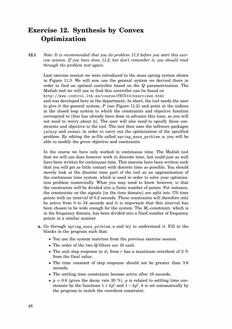
12.1 Note: It is recommended that you do problem 11.2 before you start this exer-
cise session. If you have done 11.2, but don’t remember it, you should read
through the problem text again.
Last exercise session we were introduced to the mass spring system shown
in Figure 11.3. We will now use the general system we derived there in
order to find an optimal controller based on the Q parametrization. The
Matlab tool we will use to find this controller can be found on
http://www.control.lth.se/course/FRTN10/exercises.html
and was developed here at the department. In short, the tool needs the user
to give it the general system, P (see Figure 11.2) and point at the indicesin the closed loop system to which the constraints and objective function
correspond to (this has already been done in advance this time, so you willnot need to worry about it). The user will also need to specify these con-straints and objective to the tool. The tool then uses the software packages
yalmip and sedumi in order to carry out the optimization of the specified
problem. By editing the m-file called spring_mass_problem.m, you will be
able to modify the given objective and constraints.
In the course we have only worked in continuous time. The Matlab tool
that we will use does however work in discrete time, but could just as well
have been written for continuous time. This exercise have been written such
that you will get as little contact with discrete time as possible. You should
merely look at the discrete time part of the tool as an approximation of
the continuous time system, which is used in order to solve your optimiza-
tion problem numerically. What you may need to know however, is that
the constraints will be divided into a finite number of points. For instance,
the constraints on the signals (in the time domain) are split into 170 timepoints with an interval of 0.2 seconds. These constraints will therefore only
be active from 0 to 34 seconds and it is important that this interval has
been chosen to be wide enough for the system. The Ms-constraint, which is
in the frequency domain, has been divided into a fixed number of frequency
points in a similar manner.
a. Go through spring_mass_problem.m and try to understand it. Fill in the
blanks in the program such that:
• You use the system matrices from the previous exercise session.
• The order of the two Q-filters are 10 each.
• The unit step response in d1 from r has a maximum overshoot of 2 %from the final value.
• The time constant of step response should not be greater than 3.6seconds.
• The settling time constraints become active after 19 seconds.
• p = 0.8 (gives the decay rate 20 %). p is related to settling time con-straints by the functions 1+ kpt and 1− kpt. k is set automatically bythe program to match the overshoot constraint.
48

Exercise 12
• The maximum magnitude of the control signal is umax = 6.• The maximum amplitude on the sensitivity function is Ms = 1.4 (givesat least phase margin 41.8○ and gain margin 3.5).
• We get the weights γ = 0.5 and ρ = 1.0 on the cost function J.
The constraints on the unit step response from r to d1 are visualized in
Figure 12.1.
0 5 10 15 20 25 300
0.2
0.4
0.6
0.8
1
Step Response Specifications
Time (s)
Ma
gn
itu
de
t1
t2
1+kpt
1−kpt
os
0.63
Figure 12.1 Constraints on the closed loop step response from the reference, r, to the
position of the first mass, d1. os is the maximum allowed overshoot.
b. The mass-spring system has two poles in s = 0 and is thus unstable. Inorder to get the Q optimization working, it is therefore necessary to have
a so called nominal controller that stabilizes the plant. The final controller
will then be optimized with respect to this stabilized closed loop system. In
the given tool for Q optimization, this nominal controller is set by the soft-
ware (LQG controller) and will therefore not need any of our attention. Theplots given by the program will however show two solutions, one of which
correspond to the nominal controller and one to our optimal controller.
Run the program, with the given setup, and identify which plots corre-
spond to the nominal and optimal controller respectively. What constraints
are active? A constraint is active if the solution touches this constraint in
any points.
c. Plot the Bode diagram of the controller. Can you recognize any resemblance
with any other type of controller? Can you give some intuition to any of the
dips in the magnitude plot?
49

Exercise 12
d. Every time you run the program you should be given some text similar to
this:
SeDuMi 1.1R3 by AdvOL, 2006 and Jos F. Sturm, 1998-2003.
Alg = 2: xz-corrector, theta = 0.250, beta = 0.500
Put 510 free variables in a quadratic cone
eqs m = 531, order n = 826, dim = 1725, blocks = 53
nnz(A) = 12452 + 1, nnz(ADA) = 20671, nnz(L) = 10601
Handling 2 + 2 dense columns.
it : b*y gap delta rate t/tP* t/tD* feas cg cg prec
0 : 4.52E+03 0.000
1 : -4.12E+02 2.98E+02 0.000 0.0660 0.9900 0.9900 1.13 1 1 1.4E+00
2 : -5.40E+00 2.08E+02 0.000 0.6984 0.9000 0.9000 6.00 1 1 3.5E-01
...
48 : -1.40E+02 3.90E-08 0.000 0.1878 0.9000 0.9000 0.97 43 35 1.4E-06
Run into numerical problems.
Lets not go into detail what all columns stand for, but rather look only at
the feas one. The number you end up with should ideally be 1, or at least
close by, in order for you to have a fully feasible solution (a solution thatsatisfies all constraints you have posed). If you end up with a value of −1,then you can know for sure that your optimization did not succeed. The
higher you have chosen the order of your Q-filters, the more likely it is that
the optimization problem will succeed if there are any feasible solutions to
be found. If we do not find a feasible solution, even though the order of the
Q-filters is large, this tells us that we should try to loosen our constraints
a bit if we want to find a usable controller.
Take your code and decrease NQ=n_q1=n_q2 until your problem is no longer
feasible. What constraint will fail first? What is the least order NQ you need
your Q-filters to have in order to get feasibility?
e. Increase the order of Q1 and Q2 simultaneously (NQ=n_q1=n_q2) from thevalue you received in the previous subproblem and plot NQ against cost
function value. Explain the shape of this plot and comment on how the max
value of the control signal changes when NQ increases.
f. Change the weights on the objective function and see how this alters the
solution. Also play around with the constraints to see if you can achieve an
extremely fast step response. Explain your results.
g. Go back to your original setup of constraints and objective function. Change
your maximum allowed overshoot on the step response to see how tight this
constraint can be made before the solution becomes infeasible. Can you play
around with some of the other constraints and the order of the Q-filters to
make the problem feasible again? Is it possible to have no overshoot at all?
h. (*) Take a look in the other m-files and see if you can find the closed looptransfer function matrix (Note: It will be in discrete time). Plot all 9 (Why9?) Bode diagrams. Point out at least one of these that you would havewished had a different appearance. How would you have prefered it to look
and why?
50

Exercise 12
i. (*) Change the system and see how this affects the solution. For instance,you can try to make both k and b small to see if you can make the system
very hard to control with the constraints we have have. Play around with
different constraints, weights on the objective and order of the Q-filters to
see if you can find a decent controller for the new system.
51

Exercise 13. Controller simplification
13.1 Consider a SISO system for which the pole-zero map is given in figure 13.1.
a. Determine the transfer function of the system. You can assume that the
static gain is G(0) = 1.
b. By studying the pole-zero map, it is possible to get a hint that the system
is a candidate for model order reduction. How?
c. Use a computer to calculate a balanced realization and the Hankel singular
values of the system. Perform a model reduction by eliminating the state
corresponding to the smallest singular value.
−1.4 −1.2 −1 −0.8 −0.6 −0.4 −0.2 0−1.5
−1
−0.5
0
0.5
1
1.5
Pole−Zero Map
Real Axis (seconds−1
)
Ima
gin
ary
Axis
(se
co
nd
s−
1)
Figure 13.1 Pole-zero map of the system in problem 13.1
13.2 For the system
(x1
x2
)
=(−1 0
−1 −0.5
)(x1
x2
)
+(2
1
)
u
y = (1 1 )(x1
x2
)
+ 10u
solve the following problems by hand:
a. Verify that the controllability gramian is
(2 0
0 1
)
while
(0.5 0
0 1
)
is the
observability gramian.
b. Determine the Hankel singular values.
c. Find a coordinate change that gives a balanced realization.
d. Find a reduced system G1(s) by truncating the state corresponding to thesmallest Hankel singular value.
13.3 For the same system and notation as in the previous problem, use a com-
puter for the following:
52

Exercise 13
a. Find the transfer function G(s) from u to y.
b. Compare the error maxω pG(iω )−G1(iω )p with the error bound for balancedtruncation.
c. Find a reduced system G2 by truncating both states and keeping just a
constant gain.
d. Compare the error maxω pG(iω )−G2(iω )p with the error bound for balancedtruncation.
13.4 Find a reduced order approximation of
2s2 + 2.99s+ 1s(s+ 1)2
by writing the transfer function as the sum of an integrator and a stable
transfer function, then applying balanced truncation to the stable part. You
may use a computer.
53

Exercise 14. Old Exam
14.1 Write down a state-space realization for the system
G(s) =[
1(s+1)(s+2)
s+3(s+1)(s2+6s+8)
]
14.2 A system has the transfer function G(s) = 1s+a , where a > 0. The input to
the system is white noise with spectral density Φn = 1. What is the spectraldensity of the output?
14.3 Steve is working with a process and he wants to design a controller for it.
After identifying the transfer function P(s) he decides to try a PI-controllerCPI(s) = 0.88(1 + 1
s). With the PI-controller, the disturbance response is
very poorly damped, so he adds a lead filter. The controller is now:
C(s) = 0.88(
1+ 1s
)s/1.79+ 1s/8.94+ 1.
The bode diagrams of the controller and the loop transfer function can be
seen in Figure 14.1. The disturbance response is still poorly damped. You
realize that Steve has made a serious mistake when calculating his lead
filter parameters.
a. What is Steve’s mistake?
b. Can you improve the disturbance response by adjusting the lead filter (in-cluding the gain K )? You have to follow the specifications:
• The cutoff frequency ω c must not change
• The high frequency gain of the controller must not increase
14.4 A linear model of an inverted pendulum on a cart is given by
Y(s) =
Y1(s)Y2(s)
= G(s)U(s) =
ω 20s2 −ω 201
s
U(s)
where Y1 is the pendulum angle, Y2 is the cart velocity and U (which is thecontrol signal) is the acceleration of the cart. Consider the control systemshown in Figure 14.2. The controller C1 is used to stabilize the pendulum.
Assume that a stabilizing controller has been designed and is given by
C1(s) =B1(s)A1(s)
.
a. Let us now consider design of the cart velocity loop with input r and output
y2. In order to evaluate different control designs, it is useful to analyze
the loop transfer function, Go(s) = C2(s)Gy2 ,m, where Gy2,m is the transferfunction from m to y2. Calculate Gy2,m.
54

Exercise 14
10−6
10−4
10−2
100
102
Ma
gn
itu
de
(a
bs)
Bode Diagram
Frequency (rad/sec)
10−1
100
101
102
−270
−180
−90
0
90
Ph
ase
(d
eg
)
PC
C
Figure 14.1 Loop transfer function PC and controller C in problem 14.3
.
C1(s)C2(s) G1(s)
G2(s)
G(s)
−1
−1
y1
y2
mr e
u
Figure 14.2 A block diagram for the inverted pendulum control system.
b. What can be said about performance limitations of the closed loop system
from r to y2? Notice: You do not have to design any controllers!
c. Figure 14.3 shows four plots, where one of the plots shows the sensitivity
and complementary sensitivity function of a closed loop system discussed
in problem b, with ω 0 = 1 and a particular choise of C2(s). Which plot?
55

Exercise 14
10−1
100
101
10−1
100
101
A
Frequency (rad/sec)
Magnitude (
abs)
10−1
101
103
10−2
10−1
100
101
B
Frequency (rad/sec)
Magnitude (
abs)
10−1
101
103
10−2
10−1
100
101
C
Frequency (rad/sec)
Magnitude (
abs)
10−1
101
103
10−2
10−1
100
101
D
Frequency (rad/sec)
Magnitude (
abs)
Figure 14.3 Magnitude plots of S and T in problem 6.
Motivate your answer!
14.5 Solve the following problems:
a. Consider the system
G2(s) =
s− 1(s+ 1)(s+ 2)
s
(s+ 1)(s+ 2)−6
(s+ 1)(s+ 2)s− 2
(s+ 1)(s+ 2)
.
Calculate the poles and zeros of G2(s). Are there any limitations on theachievable bandwidth?
b. Determine the RGA of G2(s) at ω = 0 rad/s and choose reasonable in-put/output pairs for decentralized control. Can we expect decentralizedcontrol to work well for low frequencies?
14.6 Assume that we can model a physical process with the following transfer
function
G(s) = (s+ a)m
(s+ b)n ,
where m = 1 < n and a, b > 0. The IMC method was used to find acontroller for this system, namely a PID controller with a lowpass filter
C(s) = K(1+ 1
Tis+ Tds)
(sTdN+ 1)
.
56

Exercise 14
Determine what n the process must have and express K , Ti, Td and N in
a, b and the design parameter λ . What PID parameters are adjustable?
14.7 Recall the the quadruple tank system that was examined in Laboratory
Exercise 2. The transfer function from the two inputs (u1, u2) to the twooutputs (y1, y2) was
G(s) =
γ 1c11+ sT1
(1− γ 2)c1(1+ sT1)(1+ sT3)
(1− γ 1)c2(1+ sT2)(1+ sT4)
γ 2c21+ sT2
This time we will approach the problem by use of Q-optimization. The ob-
jective will be to keep the control errors (e1 = r1− y1, e2 = r2− y2) low. Forthis reason we will choose r1 as well as r2 to be exogenous inputs w (seeFigure 14.4) while e1 and e2 will be our exogenous outputs z. The signalsr1, r2, y1 and y2 will all be given to the controller. Hence
z =[r1 − y1r2 − y2
]
w=[r1
r2
]
y =
y1
y2
r1
r2
Determine the transfer function matrix
[Pzw Pzu
Pyw Pyu
]
−C(s)
� �
�
-
u
z
y
w
Figure 14.4 General form of a closed loop system.
P =
Pzw Pzu
Pyw Pyu
(see Figure 14.4) for the quadruple tank system.
14.8 A MIMO system is described by the following transfer functions:
P(s) =
1
s+ 2 − 1
s+ 21
s+ 11
s+ 4
a. Calculate the zero(s) of the process.
b. Suppose that we want to control the process by selecting input and output
pairs for two SISO loops. How should we pair the input and outputs ?
57

Exercise 14
14.9 Consider the following process
G(s) = 4.2
s2 + 0.12s+ 1.
The control structure chosen is state feed-back design by minimizing the
cost function
J =∞∫
0
yTQ1y+ uTQ2u dt
and a feed-forward gain Lr such that we have the control signal
u(t) = −Lx(t) + Lrr(t).
Four different cost functions have been used and step responses from r to y
have been plotted for performance comparison. However, the plots have not
come in the correct order. Help the designer by pairing the correct weights
below and step responses in Figure 14.5. A cost function might suit several
step responses, give all alternatives! Motivate!
A. Q1 = 1, Q2 = 10 B. Q1 = 1, Q2 = 0.01C. Q1 = 100, Q2 = 1000 D. Q1 = 1, Q2 = 100
58

Exercise 14
0 2 4 6 80
0.5
1
1.5
Step response 1
Time (sec)
Am
plit
ude
0 2 4 6 80
0.5
1
1.5
Step response 2
Time (sec)
Am
plit
ude
0 5 10 15 20 250
0.5
1
1.5
2
Step response 3
Time (sec)
Am
plit
ude
0 0.5 10
0.5
1
1.5
Step response 4
Time (sec)
Am
plit
ude
Figure 14.5 Step responses for Problem 14.9
59