exchange reactions in soils - university of …lawr.ucdavis.edu/classes/ssc102/section6.pdf ·...

Soil Chemistry 6-1

Section 6 - Exchange

EXCHANGE REACTIONS IN SOILS

We have already demonstrated that soil colloids exhibit charges at the mineral surface, which arise from structural

defects and protonation reactions. Since charge balance must be maintained counter ions of opposite charged satisfy

most of the surface charges. The interaction varies from covalent bonding (specific adsorption) to weak electrostatic

interactions. Ions attracted by weak electrostatic interactions can be replaced by other similarly charge ions. This

process of stoichiometric replacement has been termed exchange. Interaction of positive ions is called cation

exchange and conversely, negatively charged ions participate in anion exchange.

Exchange reactions are rapid, if the site is solution accessible, stoichiometric, reversible, and exhibits preferences

(selectivity) among ions of differing charge and size. This section details the exchange process. Stronger covalent

interactions will be covered in the adsorption section.

Since exchange is a chemical reaction, it can be treated like any other mass action expression and an

equilibrium constant can be defined for the reaction. The equilibrium expression K has been named the selectivity

coefficient, exchange coefficient and other terms.

For the reaction: AX + B BX + A �

We may define the following selectivity coefficient:

AB

( ) ( )Selectivity coefficient = = K ( ) ( )

BX AAX B

If the value of the selectivity coefficient is >1, this implies that B is preferred over A and if K <1 then A is preferred

over B. There are several reasons that one ion may be more strongly attracted to the surface than another ion.

ION EXCHANGE SELECTIVITY

The following is a discussion of some of the reasons for differential preference.

VALENCE - The general rule is that the exchanger prefers the ion of higher valence (more properly, the charge on

the ion). However, we will see later that under some conditions, this rule can be violate.

ION SOLVATION - The exchanger will prefer the ion that is less solvated with water molecules. This rule also

takes the form of the "Iyotropic series". Another formulation is that the exchanger will prefer an ion which is

a (water) structure "breaker" over one which is a structure "maker".

Soil Chemistry 6-2


CHELATION BY EXCHANGER - Some exchangers such as proteins, humates, fulvates and polyuronides

have vicinal functional groups that can form a multidentate complex with ions. Since divalent (and higher valent)

ions generally form chelate structures whereas monovalent ions do not, the above environmental materials are

likely to show additional preference for higher valent ions.

van der WAAL'S FORCES - The exchanger will prefer the ion with the greater number of "exposed" atoms

which can form dipole-induced dipole attractive forces between the exchanger and the ion. An example of this

is the inability of mineral salts to displace polynuclear aluminum hydroxides from the interlayer of smectites and

vermiculites.

SIEVE ACTION BY EXCHANGER - Zeolites are aluminosilicate exchangers with internal channels of sizes

that permit small ions to enter but which exclude larger ions.

The Exchange Process

A number of expressions have been proposed to quantitatively describe the equilibrium between ions

in bulk solution (pore water) and ions in aqueous solution immediately adjacent to charged colloid surface

(interface). The first type is referred to as "solution phase" ions that are no different in concept from ions that

have come into solution from dissolution of salts while the second type is called "exchangeable" ions. Some of

these types of ions are thought to be loosely bound to the surface by forces in addition to electrostatic forces

while others are clearly dissociated from the surface and fully hydrated but still held in the area by electrostatic

forces. We will learn later that the boundary between the exchange "phase" in solution and the "solution" is not

sharp or distinct; hence the term diffuse layer to describe the zone in solution which includes all of the exchange

ions. Although there is a distressing vagueness to this general picture, we use a pragmatic experimental approach

which says that solution phase composition for a column of soil or sediment in a cylinder is the salt composition

of an aqueous solution that passes into the top of the column and exits the bottom of the column without

change. By definition, the exchange phase is at equilibrium with a solution of exactly known ionic composition.

Next, we extract all of the pore water (including its salt) as well as all the exchangeable ions. By subtracting the

quantity of salt ions from the total quantity of ions, the quantity of exchange ions in the sample is estimated.

Obviously, this simple approach assumes there is one type of charge in the sample, cation exchange capacity

or anion exchange capacity but not both.

Solution phase ion activities are expressed as usual:

(Ca2+) - Calcium ion activity = ?Ca[Ca2+].

Soil Chemistry 6-3


where ?Ca = the activity coefficient of calcium ion in that particular solution and

[Ca2+] = the concentration of free calcium ion in solution.

Many different nomenclature conventions are used throughout the literature to represent the exchange

phase composition in equilibrium expressions:

XCa, CaX, Ca , Ca-Clay

In addition to these obvious but unimportant differences, one must be careful to note that different

expressions have quite different dimensions. For instance, the selectivity coefficient of Helfferich (KBA), includes

terms for A and B in dimensions of moles A (and B) per liter of exchange phase fluid. It is fairly easy to

estimate the volume of water inside a bead of swollen synthetic organic resin exchanger, and since most of the

exchange capacity (the sum of the functional groups) of the bead is inside the bead, it is possible in this special

exchanger to express AX (or BX) in the dimensions given above. Obviously, it is very difficult unless one

makes some very arbitrary assumptions to estimate (in a soil-water system) an exchange phase fluid volume.

When estimated, this volume is sometimes termed an "exclusion volume", again because salt is virtually

excluded from this zone of water in the pores. Note in the selectivity coefficient expression, values of AX and

[A] are both given in moles per liter but the exchange solution is a different compartment than the salt solution

compartment (pore water). In making measurements on real columns of resin bead exchangers, the total volume

of water inside all the beads in the column, VBT is likely to be different from the total volume of all the water

in the pores, VPT between the beads. In order to calculate [A], one uses a chemical estimate of the total quantity

of salt A, QA, and VPT:

[A] = QA/VPT.

Note that later in the simplified dynamic exchanger model, Farmer Fillipi, we make the assumption that VPT =

VBT .

This difficulty (knowing VBT) is eliminated by the Vanselow convention which uses the mole fractions

of the ions in the exchanger, NA and NB, as the representing dimensions:

AA

A B

Q = N + Q Q

This does introduce another minor difficulty when the valences of the two ions, zA and zB are not equal

because the total exchange capacity in the column, CEC, in dimensions of equivalents is:

Soil Chemistry 6-4


CEC = zA QA + zB QB

Therefore, when zA ≠ zB, QA + QB ≠ constant at different QA/QB, even when CEC is constant.

Following are statements and definitions about some of the exchange expressions that have been

proposed. Their relative quality has been or can be Judged on two bases. Some expressions are preferred by

chemists because they have a solid basis in thermodynamics, i.e., they can be derived by formal chemical

thermodynamic arguments very similar to those invoked to derive expressions for acid-base dissociation, ion-pair

formation, chelation, complex formation, or solubility "products". (It is not expected at the level of this class that

the student has knowledge of chemical thermodynamic theory, but it is expected that you have already had

some experience with the working expressions derived from thermodynamics for these equilibria.)

A second criteria used to judge quality of an expression is the degree to which the expression describes

equilibria over a wide range of chemical compositional space, i.e.

from QA/(QA + QB) ~ 0 to QA/(QA + QB) ~ 1.

None of the expressions given below are really good when judged on both criteria simultaneously. From

a practical standpoint, the second criterion is certainly the most important.

THERMODYNAMIC EXPRESSIONS

A general stoichiometric reaction is.

aA + bB = aA + bB

(Note: this does not give the valences of A and B but the integer values of (a) and (b) are based on the

integer values of these valences. The main reason we write the above expression is to see what the values of

(a) and (b) should be and it is not important whether the expression is written as above or from right to left with

A and B as "reactants" rather than as "products".)

The equilibrium thermodynamic expression is:

a b

b a

( A ( B ) )K = ( B ( A ) )

where ( ) = activity of the ion in the phase.

A specific example of monovalent-divalent cation exchange in soil represented by the symbol X is:

Soil Chemistry 6-5


2 NaX + Ca2+ = CaX + 2 Na+

2+

2 2+

(CaX ) (Na )K = (NaX (Ca ))

Note that the thermodynamic K has no subscripts or superscripts. Also note that the activity of the participant

ions can be calculated with standard techniques using total concentrations of the free ions and the ionic strength

of the solution. However, there are no generally accepted techniques to calculate the activity coefficients of ions

in the exchanger phase, γ , so that for example:

( A ) = [ A ]γ

One of the first suggestions to deal with this problem was that of Vanselow who suggested that mole

fraction, Ni, of an ion in the exchange phase might be proportional to activity in the exchange phase by analogy

with the known behavior of two different elements in solid solutions such as copper and zinc in brass. Thus.

AA( A ) = Nγ

where AA

A B

Q = N + Q Q

Without calculating the γ 's, the Vanselow exchange coefficient, Kv, is given by:

baA

V abB

(B)N = K (A)N

Therefore,

aA

VbB

K = Kγγ

For the specific case of Na-Ca exchange:

2+Ca

V 2 2+Na

( )N Na = K( )N Ca

Initially, it was probably hoped that Kv would be relatively constant at different values of the ratiob

a

(B)(A)

. This turned out to be true but only over narrow ranges of the ratio. Therefore, one would expect this

to be the death of the Vanselow expression. It was not, for two reasons. First, a mole fraction is an easy

parameter to calculate from experimental data because it does not involve the additional uncertainty of the value

of VPT in a given system. Second, Gaines and Thomas developed a theory based on further thermodynamic

Soil Chemistry 6-6


arguments that lead to the estimation of K from many measurements of KV at many selected experimental

values of b

a

(B)(A)

. We will not study this theory because even though we may know K for a particular sample of

a soil or a sediment, it is not possible to use K to predict the exchange behavior of that material in the field

without also knowing each of the exchange phase activity coefficients as functions of exchange phase

composition. The cost of doing this for a soil profile by standard techniques would be exorbitant. Sparks details

the methods of deriving K from Kv because the theoretical applications of exchange equations are problematic,

less rigorous formulations have been developed to describe cation exchange in soils.

Empirical or Semi-Theoretical Expressions

1. Gapon.

+1/2

G 0.52+

[ X ] [ ]Ca Na = K[NaX] [ ]Ca

As ordinarily applied, the cation concentrations in solution are inserted in dimensions of mmol/L

(concentration, not activity), while the exchange composition is inserted in dimensions of meq/100 g of sample.

Note that the expression includes both exchangeable sodium and exchangeable calcium with a unitary exponent.

This equation was adopted by workers at the USDA Salinity Laboratory at Riverside, California to describe the

exchange behavior of Western United States soils. They then collected many soils with a variety of salinity and

Na-Ca-Mg compositions. Soluble and exchange ion compositions of each were measured. Then, the data were

plotted with NaX/(CaX + MgX) on the Y-axis and (Na+)/(Ca2+ + Mg2+) 0.5 on the X-axis. The parameter on the

Y-axis was dubbed Exchangeable Sodium Ratio (ESR) while that on the X-axis was called the Sodium

Adsorption Ratio (SAR). The "best" straight line was fitted through the data graphically giving the equation:

ESR = - 0.01 + 0.015 (SAR)

This expression is sometimes called the statistical regression equation (see Agricultural Handbook No. 60.).

Note that the slope ~ 1/KG and that this form is tantamount to assuming that

2+

2+

CaX [ ]MgK = 1 = MgX [ ]Ca

Soil Chemistry 6-7


The equation applies reasonably well to saline or saline-alkali soils dominated by smectite clay minerals,

but should not be applied without calibration to variable charge soils.

There are a number of other exchange equations in the literature that have been used to describe cation

exchange in soils. However, the discussion above will suffice to introduce you to the concept of exchange

equations and selectivity. Application of exchange equations to soil systems produce some interesting results

in relation of changes in soil moisture, and salt levels.

Dilution (or alternatively, desiccation)

Lets calculate the effect of changing salt level (dilution or desiccation) on composition of the exchange and

solution phase.

Assume:

1. Kv = 1 = constant = 2+

Ca2 2+Na

( )N Na ( )N Ca

2. ESP = % of exchange phase occupied by Na+.

ECaP = % of exchange phase occupied by Ca2+.

3. All ? = 1

Solution phase Exchange phase(Ca2+)/(Na+) ESP EcaP

.001/.001 1.58 98.4.01/.01 4.99 95.00.1/0.1 15.6 84.41.0/1.0 44.7 55.310/10 84.5 15.5

The result is that exchangeable sodium percentage is not constant. The exchanges shows increasing

preference for the lower valent ion as the concentration of both ions increase. The phenomenon has

been formalized by Schofield as the "Ratio Law".

Soil Chemistry 6-8


Exchange Composition During Desiccation of Solution Phase.

The following graphs were constructed from calculations resulting from the following models, assumptions and

protocol:

1. Initially the soil is saturated at ? = 0.385 L H20/kg soil. This solution is considered to have two different

initial compositions (mi):

a. Case 1. [Na+] = [Ca2+] = 0.005 moles/L = mi

b. Case 2. [Na+] = [Ca2+] = 0.015 moles/L = mi.

2. The exchange equation used is that due to Vanselow arranged in the following form:

2+X X

V2 2+X

[ + ] ( )Ca Na Na = K[ ( )]Na Ca

where:

(Na+) = moles Na+/L solution phase

(Ca2+) = moles Ca2+/L solutlon phase

[CaX] = moles Ca2+ in the exchange phase / kg O.D. soil

[NaX] = moles Na+ in the exchange phase / kg O.D. soil

a. Two cases are considered:1. KV = 12. KV = 5.

3. Exchange capacity of the soil is constant at 150 mmol (+)/kg O.D. soil.

4. After the first computation is performed at ? = 0.385, the soil is dried without gain or loss of electrolyte

from the system.

5. One special case is considered where KV = 1, mi = 0.015, but where the concentration of Ca2+ in solution

remains constant during drying due to the precipitation of gypsum.

6. Two parameters are calculated during the drying process which are defined as:

a. fNa in solution = equivalent fraction of Na+ in solution

+

Na 2+ +

( )Na = f2 ( ) + ( )Ca Na

b. fNax - equivalent fraction of Na in exchange phaseX

NaXX X

( )Na = f2 ( ) + ( )Ca Na

Soil Chemistry 6-9


Calculated changes in exchanger and solution phases during in situ drying.

KV = 5 KV = 1.Cai

2+ = Nai+ = 0.005 Cai

2+ = Nai+ = 0.005

? Na+ Ca2+ +Naf NaXf Na+ Ca2+ +Naf NaXf

0.385 .00500 .00500 .333 .0158 .00500 .00500 .333 .03530.340 .00549 .00575 .323 .0162 .00545 .00577 .321 .03580.300 .00603 .00661 .313 .0166 .00593 .00666 .308 .03630.250 .00690 .00810 .299 .0171 .00671 .00820 .290 .03700.200 .00812 .01040 .281 .0178 .00778 .01050 .269 .03780.150 .00997 .01430 .259 .0187 .00940 .01460 .244 .03880.100 .01320 .02230 .229 .0198 .01210 .02280 .210 .04010.050 .02100 .04720 .182 .0216 .01850 .04850 .160 .0420

KV = 1 KV = 1Ca2+ = 0.015 = constant Nai

+ = 0.015 Cai2+ = Nai

+ = 0.015.

? Na+ Ca2+ +Naf NaXf Na+ Ca2+ +Naf NaXf 0.385 .0150 .015 .333 .0611 .0150 .0150 .333 .06110.340 .0157 .015 .344 .0640 .0164 .0173 .322 .06240.300 .0164 .015 .354 .0668 .0180 .0199 .311 .06360.250 .0174 .015 .367 .0707 .0205 .0244 .296 .06550.200 .0184 .015 .381 .0750 .0240 .0313 .277 .06760.150 .0197 .015 .396 .0800 .0293 .0431 .254 .07030.100 .0210 .015 .412 .0856 .0385 .0674 .222 .07400.050 .0227 .015 .43 .092 .0604 .1430 .174 .07950.020 .0237 .015 .442 .0965 .106 .3800 .122 .0855

Volumetric Water Content (θ)

0.0 0.1 0.2 0.3 0.4 0.5

Solu

tion

Pha

se N

a fr

acti

on (

f Na+

)

0.10

0.15

0.20

0.25

0.30

0.35

0.40

0.45

0.50

Solution Na fraction in response to changing water content.

Kv = 1, m i = 5 mML-1

Kv = 1, mi = 15 mML -1 , Ca2+ constant

Soil Chemistry 6-10


Volumetric Water Content (θ)0.0 0.1 0.2 0.3 0.4 0.5

Exc

hang

e P

hase

Na

frac

tion

( f N

a+X)

0.00

0.02

0.04

0.06

0.08

0.10

0.12

Exchangeable Na fraction in response to changing water content.

Kv = 5, mi = 5 mML-1

Kv = 1, mi = 15 mML-1 , Ca2+ constant

Kv = 1, mi = 5 mML-1 Kv = 1, mi = 15 mML-1

Volumetric Water Content (θ)0.0 0.1 0.2 0.3 0.4 0.5

Solu

tion

Pha

se N

a or

Ca

(mM

L-1

)

0

10

20

30

40

50

60

Solution Ca and Na in response to changing water content.

Ca2+, Kv = 1

Na+ , Kv = 1

Ca2+, Kv = 5

Na+, Kv = 5

Soil Chemistry 6-11


BECKETT - Q/I RELATIONSHIPS

Exchange reaction and exchange capacity in soils are sources of plant nutrient such as K, Ca and Mg.

However, it is difficult to visualize how the complex interaction between ions, exchange capacity and extraction

of nutrients by plant affect nutrient supplies. Beckett developed a technique and theory to examine the buffer

capacity of soils with respect to potassium. The theory is based on exchange reactions between Ca, Mg, and

K. Beckett called the buffering capacity of the soil with respect to potassium quantity-intensity relations. In this

concept Q stands for quantity, I stands for intensity. Although the following from Beckett was derived for

assessing potassium status in soils, it can be generalized to a large number of other systems. These are

summarized and presented in the following table.

Summary Table of Quantity-Intensity Buffering Relationships.

System Q I Buffer Index (dQ/dI)Acid-base Ca or Cb pH dC/dpHthermal calories temperature dQ/dT

soil water % water in soil vapor pressure d?/dPH2O

soil nutrient -K+K KAR

K

d Kd AR

The following graph illustrates the concept of Q/I for soil solution ions and soil buffering capacity as derived from

the changes in Q in relation to changes in solution ion levels.

Solution Intensity ( I) 0 1 2 3 4 5 6

Ads

orbe

d Q

uant

ity

( Q

)

0

2

4

6

8

Soil A

Soil B

∆ Q

∆ IA ∆ IB

BC = (∆ Q / ∆ Ι )

BCA > BCB

Soil Chemistry 6-12


Beckett's proposal for evaluation of soil potassium status is based on a mass action exchange equation:

2+

+

2+ 22+ +M

2+2K 2++

[ + ] (Mg )Ca K = K[ ( + )Mg] CaK

where ( ) = activities, and [ ] = concentrations. Take the square root and rearrange:

2+

+

2+ 0.52+++

2+ 0.5 0.52+ MK

( ) [ + Mg ]CaK[ ] = K( + (Mg ) )Ca K

In the above, the Q or quantity term for potassium = +[ ]K while +

K2+ 0.52+

( )K = AR( + Mg )Ca

the activity

ratio in solution is the I or intensity term for potassium.

If Q is plotted as a function of I, the slope should represent the ratio of exchangeable calcium plus

exchangeable magnesium divided by the square root of the selectivity coefficient.

However, Beckett added an additional feature permitting the examination of the change in exchangeable

potassium and obviating the need to directly measure +[ ]K . Suppose that ARK is changed so that ARK

increases. The equation predicts an increase in +[ ]K = + K∆ . This new condition could be represented as

follows:

2+

+

0.5+

2+2++

+ +2+ 0.5 0.52+ M

K

K( ) + - MgCaK2

[ ] + [ ] = K K( + ( Mg ) )Ca K

∆ ∆

Rearranging:

2+

+

0.5+

2+2++

+ +2+ 0.5 0.52+ M

K

K( ) + - MgCaK2

[ ] = - [ ]K K( + (Mg ) )Ca K

∆ ∆

If +[ ]K

2∆

<< 2+2+[ + ]MgCa then the slope of a plot of +[ ]K versus ARK should be approximately

constant and this function should approximate a straight line with a negative intercept equal to exchangeable

potassium in the original sample.

The procedure is to weigh out several 5 g soil samples. To each is added a KCl and CaCl2 solution of

designed potassium and calcium concentration. Fifty mL of solution is added to each soil sample and the flask

Soil Chemistry 6-13


is shaken. Then it is centrifuged or filtered and K+, Ca2+ and Mg2+ are measured. Ionic strength (µ) is calculated

and activity coefficients for the three cations are calculated from by the extended Debye-Hückel (or other)

equation. These values are used to calculate ARK. Differences between the final equilibrium solution K+ and the

initial solution K+ are K

? (? K )? A R

due to adsorption or desorption of exchangeable K. The x axis value is a measure

of available K+ or the intensity of labile K in a soil. The potential buffering capacity (PBCK) is a measure of the

ability of the soil to maintain the intensity of K in soil solutions. It is proportional to CEC. Low PBCK indicates

a need for frequent fertilization. KX is a measure of specific sites for K, and ?Ko is the labile or exchangeable K.

A typical Quantity/Intensity (Q/I) plot from Sparks and Liebhardt 1981. Effects

of Long-term Lime and Potassium Applications on Quantity-Intensity

Relationships in Sandy Soil. SSSAJ 45:786-790.

∆K+ (

cm

oles

(+) k

g-1)

∆ Κο

AReK

Kx

Slope = PCBK

2 20.5( )

K K

Ca Mg

aAR

a a+

+ +

=+

∆ (∆K) ∆ ARK

Soil Chemistry 6-14


The figure on the left illustratesthe difference between two soil

with very different potassium bufferingcapacities.

[Note that this older data uses meq/100gand that Mg is not included in the AR].

Source: G. W. Thomas (1974)-Chemical Reactions Controlling SoilSolution Electrolyte Concentration.IN Carson the Plant Root and Its

Environment.

Soil Chemistry 6-15


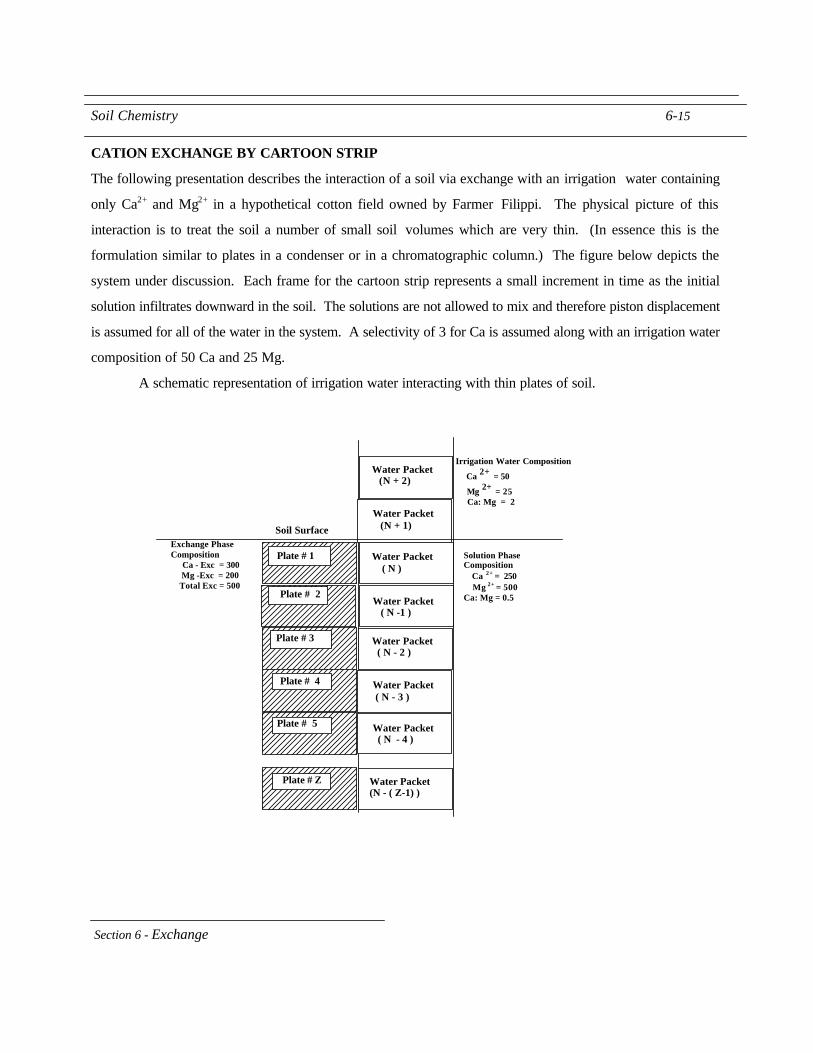
CATION EXCHANGE BY CARTOON STRIP

The following presentation describes the interaction of a soil via exchange with an irrigation water containing

only Ca2+ and Mg2+ in a hypothetical cotton field owned by Farmer Filippi. The physical picture of this

interaction is to treat the soil a number of small soil volumes which are very thin. (In essence this is the

formulation similar to plates in a condenser or in a chromatographic column.) The figure below depicts the

system under discussion. Each frame for the cartoon strip represents a small increment in time as the initial

solution infiltrates downward in the soil. The solutions are not allowed to mix and therefore piston displacement

is assumed for all of the water in the system. A selectivity of 3 for Ca is assumed along with an irrigation water

composition of 50 Ca and 25 Mg.

A schematic representation of irrigation water interacting with thin plates of soil.

Plate # 1

Plate # 2

Plate # 3

Plate # 4

Plate # 5

Plate # Z

Water Packet (N + 2)

Water Packet (N + 1)

Water Packet ( N )

Water Packet ( N -1 )

Water Packet ( N - 2 )



Water Packet (N - ( Z-1) )

Soil Surface

Irrigation Water Composition

Ca 2+ = 50

Mg 2+ = 25 Ca: Mg = 2

Exchange PhaseComposition Ca - Exc = 300 Mg -Exc = 200 Total Exc = 500

Solution Phase Composition Ca 2+ = 250 Mg 2+ = 500Ca: Mg = 0.5

Soil Chemistry 6-16


Conditions in thewater packetsand soil solidphase asirrigation waterof knowncompositioninfiltrates into asoil pore.

Soil Surface

Plate # 1

Plate # 2

Plate # 3

Incoming irrigation water

Water Packet

Water packet

Water packet

Water Packet

Condition in the soil Constant Exchange Cap. Selectivity Coefficient = 3 Volume of exchange phase equal to volume of water packets.

Volume of solution packet equal to volume of exchangephase

Water equilibrates with the exchange phase and doesnot mix with upper or lower water packets

Piston displacement of water is assumed

Known and constant composition

Initial composition of all water packets in thesoil are the same.

Drainage water has the composition of the last water packet

Soil Chemistry 6-17


Plate 1 Ca-Ex = 300Mg-Ex = 200

Soil Solution Ca = 250 Mg = 500

Frame 1

Explanation


Soil SolutionCa = 250 Mg = 500

Exchanger phase (left ) is at equilibrium with the solution phase (right) in the surface of a field about to be irrigated with with water containing 50 Ca and 25 Mg. KCa

Mg = 3 = (CaX )(Mg) / (MgX) (Ca)

Water Packet 2Ca = 50 Mg = 25

Frame 2


Soil Solution ( WP 1)Ca = 250 Mg = 500

Farmer Fillipi applies water to the field. Note thatthis water is more dilute than the soil water and thatCa/Mg in the irrigation water is 2.0 while in the soilwater it is 0.5. The incoming water is called waterpacket 2 (WP2). The thin layer of soil is called plate 1 (PL 1). A plate is of the order of 3-4 mm thick.


Frame 3



Water Packet 3 Ca = 50 Mg = 25

The packet of water displaces an equal volume of soil water without mixing. No exchange or reaction has occurred (yet) between the incomingwater and the exchangeable ion on the soil. The equilibrium values of the exchangeable and solution ions can be calculated knowing the selectivity coefficient and including a mass balance statement. The derivation is shown on the following pages.

Soil Chemistry 6-18


Plate 1 Ca-Ex = 321.8Mg-Ex = 178.2

Frame 4

Explanation



Frame 5

Plate 1 Ca-Ex = 321.8Mg-Ex = 178.2

Water Packet 2 Ca = 28..2 Mg = 46.8

A new water packet (WP 3) is position to infiltrate into the soil displacing WP2 to the next soil plate PL 2.

Water Packet 2Ca = 28.2 Mg = 46.8

Frame 6



Water Packet 3 Ca = 50 Mg = 25

The water packet (WP3) has entered and displacedthe previous equlibrated packet. The displace packetis now opposite another volume of exchanger having the same composition as Plate 1 before infiltration of water packet 2 (WP2). The system is not at equilibrium



The system comes to equilibrium. Values in Frame 3 must be used to solve equation 8 of the Ca-Mg derivation sheet to give these equilibrium values.

Plate 1 Ca-Ex = 321.8Mg-Ex = 178.2

Soil Chemistry 6-19


Plate 1 Ca-Ex = 340.6Mg-Ex = 159.4

Frame 7

Explanation

Plate 2 Ca-Ex = 302.8Mg-Ex = 197.2


Frame 8

Plate 2 Ca-Ex = 321.8Mg-Ex = 178.2

Water Packet 3 Ca = 26.1 Mg = 48.9

A third packet enters and all layer have come to a new equiilibrium


Water packet 2Ca = 25.39Mg = 49.6

Both layers come to equilibrium.

Plate 1 Ca-Ex = 356.6Mg-Ex = 143.4

Plate 3 Ca-Ex = 340.6Mg-Ex = 159.4


Plate 4 Water Packet 1Ca = Mg =

What is the compostion of plate 4 and water packet 1 in Frame 8 ?

Soil Chemistry 6-20


DERIVATION OF THE Ca-Mg EXCHANGE FUNCTION

A. Selectivity coefficient:

2+CaMg 2+

[ Ca ] [ ]Mg = K[ Mg ] [ ]Ca

(1)

B. Mass balance:

2+T[ Ca = [ Ca ] + [ ]] Ca (2)

2+T[ Mg = [ Mg ] + [ ]Mg] (3)

C. Exchange capacity of the exchanger T[ R ] is constant, and therefore:

T[ R = [ Ca ] + [ Mg ]] (4)

D. (1), (2), (3) and (4) can be rearranged into a polynomial in [Ca] by rearranging (2), (3), and (4):

2+ 2+T T T[ ] = [ Mg - [ R + [ Ca - [ ]Mg ] ] ] Ca (5)

2+T[ Mg ] = [ Mg - [ ]Mg] (6)

( )2+T T T T[ Mg ] = [ Mg - [ Mg - [ R + [ Ca - [ ]] ] ] ] Ca (6a)

2+T[ Ca ] = [ Ca - [ ]] Ca (7)

E. Substituting (5), (6a), and (7) into (1) and rearranging:

22+ 2+A [ + B [ ] + C = 0]Ca Ca (8)

where:CaMgA = ( -1 )K (9)

Ca CaMg MgT T TB = [ - 1][R - [ - 2 ][ Ca + [ Mg ] ] ]K K (10)

( )T T T TC = ([ R - [Mg ) - [Ca [Ca] ] ] ] (11)

Soil Chemistry 6-21


DERIVATION OF THE Ca-Na EXCHANGE FUNCTION

A. Selectivity coefficient:

2+CaNa 2 2+

[ Ca ] [ ]Na = K[ Na [ ]] Ca

(1)

B. Mass balance:

2+T[ Ca = [ Ca ] + [ ]] Ca (2)

+T[ Na = [ Na ] + [ ]] Na (3)

C. Exchange capacity of the exchanger T[ R] is constant, and combined with the electrical neutrality

condition:

T[ R = 2 [ Ca ] + [ Na ]] (4)

D. (1), (2), (3) and (4) can be rearranged into a polynomial in [Na]. This is arbitrary. It could also be

rearranged into a polynomial in any of the other variables. Equation (2), (3), and (4) are first rearranged

into:

T[ R - [ Na]][ Ca ] =

2(5)

+T[ ] = [ Na - [Na ]]Na (6)

2+T T[ ] = [ Ca - 0.5 [ R + 0.5[ Na ]] ]Ca (7)

E. Substituting (5), (6), and (7) into (1) and rearranging:

3A [ Na + B [Na ] + C [ Na ] + D = 0] (8)

where: CaNaA = 0.5 ( + 1 ) K (9)

Ca CaNa NaT T T TB = [Ca - 0.5 [ R - 0.5 [ R - [ Na ] ] ] ]K K (10)

2T T TC = [ R [Na + 0.5[Na] ] ] (11)

2T TD = - 0.5[ R [ Na ] ] (12)

Soil Chemistry 6-22


Ca -Mg EXCHANGE by FARMER FILLIPI

Behavior in Plates 1 & 2.

Plate 1Water Packet # CaX MgX [Ca] [Mg]

1 300 200 250 500.2 321.8 178.2 28.2 46.8.3 340.6 159.4 31.2 43.8.4 356.6 143.4 34.0 41.0....4 428.6 71.4 50 25

Plate 2Water Packet # CaX MgX [Ca] [Mg]

0 300 200 250 500.1 300 200 250 5002 302.8 197.2 25.39 49.63 307.9 192.1 26.1 48.9...4 428.6 71.4 50 25

Behavior of Water Packet #2Plate # CaX MgX [Ca] [Mg]

0 50 251 321.8 178.2 28.2 46.82 302.8 197.2 25.4 49.63 300.3 199.7 25.04 49.96...4 300 200 25 50.00

Soil Chemistry 6-23


Water Packet Number 0 5 10 15 20 25 30

Exc

hang

eabl

e C

a or

Mg

50

100

150

200

250

300

350

400

450

Mg Ex - Plate 7

Mg Ex - Plate 1

Kv = 3 CaEx - Plate 1

CaEx - Plate 7

Water Packet Number

0 5 10 15 20 25 30

Solu

tion

Ca

or M

g

20

25

30

35

40

45

50

55

Ca - Plate 1

Mg - Plate 1

Ca - Plate 3

Mg - Plate 3

Solution Ca or Mg in relation to Water Packet Number

Soil Chemistry 6-24


QUANTITATIVE DESCRIPTION OF SOIL SOLUTION - COLLOID INTERFACE

The figure above illustrates the general concepts of a cation distribution around a charged particle.

Assuming that the particle is negatively charged, anions are repelled from the surface and cations are

attracted to the surface. This attraction and repulsion extend outward into the solution bathing soil colloids to

a greater or lesser extent depending on the charge on the colloid, the ionic strength of the bathing solution, the

nature of the interaction between the cations, the anions and the surface, and the valence of the cations and

anions. At come distance from the colloid, the field of the colloid is not expressed and the repulsion and

attraction of cations and anions is zero. This point is called bulk solution. Since electrical neutrality must be

maintained in bulk solution the charge in any volume element from negative ions is equal to the charge in this

volume element from positively charged ions.

Numerically this is: i i i iz m z m+ + − −= and if we use the politically incorrect notation of equivalents

then i i iz m n= and i in n+ −= . If we use the notation that in the bulk solution n = no, then relative to no,

n+ increases as we approach the negative colloid and n- decreases.

Soil Chemistry 6-25


This behavior is analogous too and well illustrated by for the distribution of gases in a gravitational field. To

help us develop a feel for the colloidal system, we will examine the behavior of gases in the earths gravitational

field. In this case gases decrease in relation to the distance from the earth’s surface. If we designate no as the

value of the gas concentration at the earth’s surface, we can develop a model of the gas distribution.

The Barometric Formula and Analogy

o

mghn = n exp

kT −

(1)

n = the number of gas atoms per cubic centimeter at height h

no = the number of gas atoms per cubic centimeter at h = 0, (earth's surface)

m = the mass of the atoms

g = the gravitational constant

k = the Boltzmann constant

T = absolute temperature ( Ko )

mgh = the gravitational potential of the gas atoms

kT = the thermal or kinetic energy of the gas atoms (escaping energy)

Thus gases are distributed in around the earth in relation to their thermal energy (kT) or escaping

tendency and the gravitational attraction (mgh). By a similar analogy, ions are distributed in an electrical field

around a charged colloid in relation to two opposing forces.

The Boltzmann Expression for Ions in an Electrical Field

++ o

c z = exp- n nkT

ψ

(2)

-- o

| z | c n = n exp

kTψ

(3)

n+ = local cation concentration

: ions cm-3

n- = local anion concentration

Soil Chemistry 6-26


: ions cm-3

no = concentration of cations and anions where ? = 0

: ions cm-3

z+ = cation valence

: electrons ion-1

z= absolute value of the anion valence

: electrons ion-1

c = the charge on the electron = 1 unit of charge =

4.8 * 10-10 statvolts electron-1

? = local electrical potential, the sign of ? is negative for negatively charged

particles.

: statvolts

Note 1 statvolt = 300 volts

zic? = electrical potential of the ion

: ergs ion-1

Note: 1 statvolt* statcoulomb = 1 erg

Define a convenience parameter (y):

i c zy = kT

ψ

(4)

then from (2) and (3):

+o + on = n exp(-y) or n = n ye− (5)

- o - o = exp(y) or n = nn n ye (6)

Introduce the Poisson equation from classical electrostatic theory:

2

2

4d = - d x D

ψ πρ(7)

x = the normal distance from a flat surface

D = the dielectric constant ? 80

Soil Chemistry 6-27


: statcoulombs cm-1 statvolts-1

? = local net charge density

? = is defined as the difference in charge in any volume element found by

summing the positive and negative charges in that volume element.

= i i (z c n )Σ (8)

: statcoulombs cm-3

substituting for ? in (7) yields:

2i

o2

4 c d z = - c n exp - d x D kTiz

ψ π ψ ∑ (9)

If we assume that the solution contains a single symmetrical electrolyte we may rewrite (9) to give:

2

i o i o i2

4 | | c | | | | c d z n z n z = - exp - - expd x D kT kT

ψ π ψ ψ

(10)

Introducing y from (4) after finding 2

2

ydd x

and recalling that exp( y ) - exp( -y )

sinh y = 2

we can

rewrite (10) as:

2 2 2i o

2

y 8 sinh(y)d c z n = d x D k T

π(11)

Since there are a number of constants in equation (11), it is convenient to introduce the convenience

parameter kappa squared:

22i o2 8 cz n =

DkTπ

κ (12)

having units of cm-1

22

2

yd = sinh (y)d x

κ (13)

Applying an integrating factor to both sides and using the boundary conditions that at x = ∞, y = 0 and

dy/dx = 0 it can be shown:

dy y = 2 sinh

dx 2κ

(14)

Soil Chemistry 6-28


Adding that y = yo at x = 0, and after some manipulations (14) may be integrated to the working equation:

a + exp ( x)y = 2 ln - a + exp ( x)

κκ

(15)

where io oo

| | c y za = tanh and = y4 kT

ψ

we proceed by introducing the space charge ( s ) which is equal and opposite to the surface charge , and has

units of: statvolts cm-2

0 = dxσ ρ∞∫ (16)

Substituting for (?) from (7) into equation (16) yields:

2

20

D d = - dx4 dx

ψσπ

∞

∫ (17)

which after some manipulations integrates to:

i o o4 c | | yz n = - sinh2

σκ

(18)

If we again introduce a convenience parameter J defined as :

i0.522

i

4 | | czJ = 8 cz

DkTπ

(19)

introducing the constant makes it easier to examine the relation between ( s) and surface potential.

Remember that surface potential is contained in the yo term.

oo

y = -J sinh n

2σ

(20)

It has been shown that for variable charge surfaces:

zpc

PDIo

PDI

kT a = lnz c a

ψ

(21)

where

oψ = surface potential of the colloid

PDIa = solution activity of the potential determining ion

Soil Chemistry 6-29


zpcPDIa = the solution activity of the potential determining ion at the point of zero charge

(zpc)

- Log µ

1.0 2.0 3.0

Per

cent

Dis

soci

ated

80828486889092949698

100I. S. Effect on Acetic Acid Dissociation

Distance from Surface ( nm)0 10 20

Con

cent

ratio

n (m

M L

-1)

0.0

2.0

4.0

6.0

8.0

10.0

Montmorillonite z = 1

mo = 1 mM

Soil Chemistry 6-30


Distance from Surface ( nm)0 10 20

Con

cent

rati

on (m

M L

-1)

0.0

20.0

40.0

60.0

80.0

100.0

120.0

Montmorillonite z = 1

mo = 1 mM

mo = 100 mM L-1

m+

m-

m-

m+

Distance from Surface ( nm)0 2 4 6 8

Con

cent

rati

on (m

M L

-1)

0

50

100

150

200

250

300

350

Montmorillonite

mo = 100 mM L-1

m+, z = 2

m-, z = 1

m- , z = 2

m+ , z = 1

Soil Chemistry 6-31


Distance from Surface ( nm)0 10 20 30 40

Pot

enti

al ,

ψ

( - m

illiv

olts

)

0

50

100

150

200Montmorillonite

z = 1, mo = 100 mM

z = 2, mo = 1 mM

APPENDIX FOR DDL

An understanding of soil electrical properties necessitates a recollection and understanding of some basic

physical science concepts. This review section is designed to reacquaint you with some concepts from physics

which are important for an understanding of DDL and other related surface phenomena.

ELECTRICAL POTENTIAL

Electrical potential (?) is a measure of the work required to move a charge in an electrical field. More

precisely, electrostatic potential at any point in space is defined as the work done to transport a unit positive charge

from infinity (a point outside the electrical field) to a point within the field. Work is done when the unit charge is

transported near a charged particle because the particle exerts an electrical force on the charge being transported.

This situation is illustrated in the following diagram:

Soil Chemistry 6-32


Positively chargedsphere

+

Direction of transport Direction of field

Unit positive charge

For a charged particle where E is the electric field or force operating on a unit charge and x is the distance

of transport, the electrical potential (?) is the product of the field (E) and the displacement x.

| | = E * xψr r

(1)

where: x = the displacement

E = the electrical field

? = the electrical potential

If the particle is positive then work is done by some external agent and the potential is taken to be positive.

Conversely, for a negative particle (the common soil situation) the potential is taken to be negative. Potential is

developed when charges are separated. Any separation of charge requires work and therefore develops a potential.

An example taken from Newman (1973) [Electrochemical Systems, Prentice Hall] illustrates the point well.

Newman estimates the 2 (1 cm in radius) metal spheres separated by 10 cm and charged to an average capacity

of 10 µC cm-2 develop a potential of 2*108 volts.

Since both the electric field and displacement are vector quantities, the product E xr r

is negative (i.e.

A B = A B cos θr r

where ? is the angle between the vectors. In this case the angle is + 180 and cos ? = -1.

Therefore, in a uniform electrical field:

x = - E xψ (2)

If E is functionally dependent on x, and the relationship is known equation (2) becomes:

x

x = - E d xψ∞∫ (3)

The relationship between E and distance can be derived from Coulomb's Law. In a vacuum Coulombs law

takes the form:

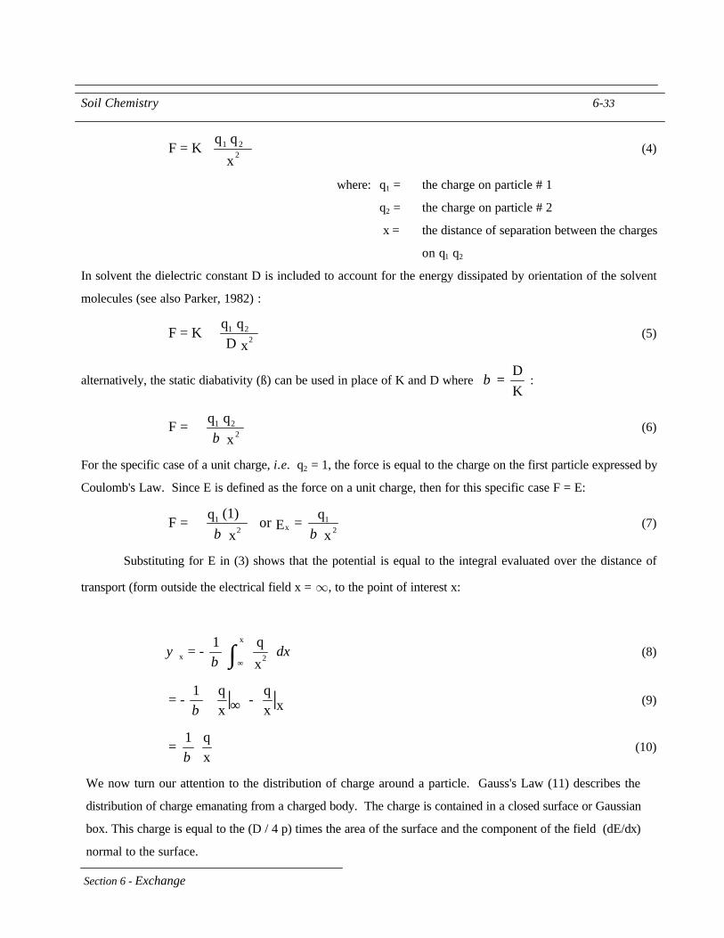
Soil Chemistry 6-33


1 22

q qF = K

x

(4)

where: q1 = the charge on particle # 1

q2 = the charge on particle # 2

x = the distance of separation between the charges

on q1 q2

In solvent the dielectric constant D is included to account for the energy dissipated by orientation of the solvent

molecules (see also Parker, 1982) :

1 22

q qF = K

D x

(5)

alternatively, the static diabativity (ß) can be used in place of K and D where D

= K

β :

1 22

q qF = xβ

(6)

For the specific case of a unit charge, i.e. q2 = 1, the force is equal to the charge on the first particle expressed by

Coulomb's Law. Since E is defined as the force on a unit charge, then for this specific case F = E:

1 1x2 2

(1) q qF = or = E x xβ β

(7)

Substituting for E in (3) shows that the potential is equal to the integral evaluated over the distance of

transport (form outside the electrical field x = ∞, to the point of interest x:

x

x 2

1 q = -

xdxψ

β ∞

∫ (8)

x1 q q

= - - x x| |

β ∞

(9)

1 q=

xβ(10)

We now turn our attention to the distribution of charge around a particle. Gauss's Law (11) describes the

distribution of charge emanating from a charged body. The charge is contained in a closed surface or Gaussian

box. This charge is equal to the (D / 4 p) times the area of the surface and the component of the field (dE/dx)

normal to the surface.

Soil Chemistry 6-34


Dq = - (A)

4d

d xπ(11)

where A = the Gaussian area

Schematically, the model for Gauss's Law applied to a flat particle is shown below (after Bockris and Reddy,

1970) [Modern Electrochemistry Plenum Press, New York].

P a r t i c l e s u r f a c ex = 0

G a u s s i a n b o x e n c l o s i n g d i f f u s e c h a r g e , q d

U n i t a r e a

x = i n f i n i t y

Choosing the enclosed area to be a unit value and rearranging gives:

d 4 (1) = - q

d x Dψ π

(12)

In ionic media (q) is equal and opposite to the charge imbalance caused by excess of counter-ions (ions

of charge opposite to the surface) over co-ions (ions of the same charge as the surface). Total charge is equal

to the summation of charge imbalance for each volume element of the Gaussian box.

x = 0q = - d xρ

∞∫ (13)

Substituting from (12) for q and rearranging yields:

x = 0d 4 = d x

d x Dψ π

ρ∞∫ (14)

Differentiating both sides of the equation yields Poisson's Equation in one dimension that describes the

divergence of the electrical potential gradient in relation to charge density.

2

2 4d = - d x D

ψ π ρ (15)

Soil Chemistry 6-35


Poisson's Equation describes the behavior of electrical potential around a charged particle. Poisson's

Equation is also used in the derivation of the Debey-Hückel Theory of ion-ion interaction. [see K.L. Babcock.

1963. Theory of the Chemical Properties of Soil Colloidal Systems at Equilibrium, Hilgardia 34: 417-542.]

As you know from lecture and the previous material, Poisson's Equation along with the Boltzmann

Equation are the fundamental equations used in the Gouy-Chapman derivation of DDL.

Soil Chemistry 6-36


MODIFICATIONS TO DDL

There are several assumption inherent in the Gouy-Chapmand model which limit its application. Forexample, the dielectric constant is assumed to be constant from bulk solution up to the particle surface. Poisson's equation is derived for point charges; therefore, ion crowding at the surface can not be accommodatedand ridiculously high concentrations are predicted for some conditions. Adamson (1976, p. 201) (PhysicalChemistry of Surfaces 3 Ed. Wiley-Interscience NY) calculates that given a surface potential of 300 mV anda bulk concentration of 1 mM L-1, the surface concentration would be 160 M L-1. Specific chemical interactionsbetween the surface and the counter ions are not build into the model. These limitations and others have beendiscussed by Bolt (1955). (Analysis of the Validity of the Gouy-Chapman Theory for the Electric DoubleLayer. J. Colloid. Sci.10: 206-218.) Bolt found that many of the assumption in the model compensated forone another. However, in many situations, refinement of the basic Gouy-Chapman model is necessary.

In 1924, Stern proposed a modification which incorporates a layer of strongly adsorbed ions next tothe surface. These adsorbed ions (specifically sorbed ions) may be partially or completely dehydrated. The SternLayer is visualized to behave like a molecular condenser and the potential drop across the layer is linear. Beyondthe Stern Layer, the ion swarm is described by the Gouy-Chapman model. A simple Stern Model is illustratedbelow.

-

-

-

-

-

+

+++

+

+

++

+

+

+

+

+

+ +

+

+

+

+

+

++

+

+

++

+

Stern Layer

Diffuse layer

Distance from surface 0 20 40 60 80 100

Pote

ntia

l, ( ψ

)

50

70

90

110ψο Surface potential

ψδ Stern layer potential

ψd Diffuse layer potential

Particle

Diffuse layer - potential described by Gouy- Chapman ModelStern Layer

Soil Chemistry 6-37


Review Questions

1. What is SAR and SARfree ? How are SAR and ESR related?

2. What assumption about the behavior or Ca and Mg is inherent in the SAR formulation?

3. What is the idea behind the Q/I relationship of Beckett? How are Ca and Mg related in this model?

4. As a soil solution is diluted, the higher valent ion is preferred by the solid phase. What predicts this

result?

5. What factors control the solid phase composition during exchange reactions?

6. What is the suggestion of Vanselow relative to exchange equations?

7. In relation to exchange reactions, what is hydrolysis?

8. In some CEC procedures alcohol is used to remove the excess soluble salts why alcohol and not water?

9. What is a selectivity coefficient?

20. How are KCa-Mg and KMg-Ca related?

21. Do all exchange sites exhibit the same affinity for H+?

22. What are the general steps in measuring CEC? Why is it called an operationally defined measurement?

23. What two forces are acting on an ion in the Gouy-Chapman model of the double layer?

24. How does ionic strength and charge affect the double layer thickness and flocculation dispersion

behavior of a colloidal system?

25. How are anions and cations distributed near a charged surface?

26. How do charge and potential vary with respect to solution concentration for constant charge and

constant potential surfaces?

27. How will CEC vary with ionic strength and pH in soils systems.

28. What is bases saturation? What is abhorrent about the term?

29. Why is there confusion about the place of H+ in the replacement series?

30. CEC is not equal to the space charge sigma (σ). Why?

exchange reactions in soils - university of …lawr.ucdavis.edu/classes/ssc102/section6.pdf ·...

Documents