CMIS 342 Revised: 02/07/2016

Page 1 of 12

Excel Case #2: Mark’s Collectibles, Inc.1

Case Description and Instructions SKILLS CHECK

You should review the following areas:

SPREADSHEET SKILLS

Import External Data COUNTA Function COUNTIF Function AVERAGE Function MAX Function MEDIAN Function MIN Function

SUM Function Pivot Tables Pivot Charts Cell Formatting Worksheet Formatting Insert Worksheet Data Range Names

Case Overview Several years ago, small, stuffed animals called Tree Point Babies became very popular

with collectors. Each month Tree Point Babies issues several new stuffed animals. Over the

years, demand for retired Tree Point Babies has grown. This has led collectors to purchase

many of these stuffed animals in the hopes that the stuffed animals can be resold at a later

date for a profit.

Mark Allan is the owner of Mark’s Collectibles, a newly established online reseller of the very

popular Tree Point Babies stuffed animals. In an effort to widen his market for reselling these

stuffed animals, Mr. Allan has built a small Web site hosted by a Web service provider,

showing high-quality images of his available Tree Point Babies. Periodically, Mr. Allan

receives a data file downloaded from his Web hosting service that contains data about visitor

traffic at his website. He would like to utilize this data to glean insights on visitor usage of his

website. Unfortunately for Mr. Allan, the downloaded data are not in a useful format;

fortunately for you, Mr. Allan hires you to make sense of the data in the file and use the data to

prepare a Site Statistics Analysis worksheet that is useful to him.

The Site Statistics Analysis worksheet will provide Mr. Allan with information about his Web

site’s visitors, including the number of visited pages, types of operating systems and browsers his visitors are using, length of time spent in each visit (i.e., visit durations), and more. In addition to preparing the Site Statistics Analysis worksheet, you will use the worksheet data to create additional tables and charts to show Mr. Allan information, such as the number of pages

1 This case is based on Lisa Miller (2009), MIS Cases Decision Making with Application Software, Fourth

Edition, Pearson Prentice Hall, Upper Saddle River, New Jersey.

CMIS 342 Revised: 02/07/2016

Page 2 of 12

viewed by month, average visit duration by month, and the most popular Web browsers used

by visitors to his site.

Scenario Details Mr. Allan pays a nominal fee to a Web hosting service to host his Web site. As part of its

service, the Web hosting service provides Mr. Allan with a text file containing traffic

statistics for this Web site. Figure 1 shows a sample of this data. As Figure 1 shows, the text

file is not in a useful format, so you have been hired to format this data into a useful

worksheet for Mr. Allan.

Figure 1: A Sample of Data from Web Site Statistics Text File

IP Address Operating

System Browser

Site Connection

Add to Favorites

Entry Exit Bandwidth Viewed

Page

999.010.210.133 Windows MS Internet

Explorer DuckDuckGo Yes 42186.47638 42186.49344 400 4

999.250.150.140 Linux Chrome Yahoo No 42189.47352 42189.48189 1 3

999.111.233.190 Windows Firefox WOW Yes 42189.58203 42189.60697 250 2

999.140.152.160 Windows MS Internet

Explorer Ask No 42191.4299 42191.44541 750 15

999.180.007.222 Macintosh MS Internet

Explorer Dogpile No 42191.61228 42191.62361 255 4

Mr. Allan gives you the most recent text file containing his Web site’s traffic data and asks

you to import the data into an Excel worksheet. To improve the appearance of the data,

Mr. Allan asks you to properly format the data in the worksheet. For instance, you should

apply a time format that will display the dates and times of visitor entries and exits in a

more user-friendly format. He also asks you to include a header in the worksheet,

specifically requesting that the date range of the file’s content be included in the header

lines.

Mr. Allan wants each row of data to be assigned a visitor number. The visitor number is

intended to help him quickly determine the number of visits his Web site has received; this

number is not intended to uniquely identify each visitor. Mr. Allan wants the Visitor

Number column to be the leftmost column in the worksheet.

For each visit, Mr. Allan wants to know the visit duration. Mr. Allan knows that the first 10

seconds of the page visit are critical for the user’s decision to stay or leave. The longer a

user is on the page, the more likely they will stay and, hopefully, purchase something. As

you study the imported data, you see that the entry and exit times for each visit are

included, so you tell Mr. Allan you will calculate and include a Visit Duration column. In

fact, as you study the raw data, you realize there are other statistics (e.g., average, most

frequently occurring) that can be drawn from the raw data. You discuss those with Mr.

Allan and include the ones he says he wants.

CMIS 342 Revised: 02/07/2016

Page 3 of 12

Design Considerations

To design the spreadsheet needed, you will create a workbook with one main worksheet.

Then, you will create additional worksheets as requested in the instructions provided by

your instructor.

Although you are free to work with the design of your workbook, the worksheet should

have a consistent, professional appearance. You should use appropriate formatting for the

cells and worksheets.

Case Questions and Deliverables

Your instructor will provide specific directions for completing this case. In addition to an

Excel Workbook, you may be asked to respond to specific questions that will require you to

interpret the outputs of your worksheet, to perform additional analyses by modifying key

inputs, to create new charts or graphs, or to add additional worksheets.

CMIS 342 Revised: 02/07/2016

Page 4 of 12

Excel Case #2: Mark’s Collectibles, Inc.

Instructions

Be sure to begin this assignment by downloading the text file

(SiteStatistics4v15.txt) containing the data you will import into your

worksheet! Download and save a copy of that file to begin your work.

Case Background and Scenario: Read the background information about Excel Case 2: Mark’s

Collectibles, Inc. to grasp the business situation you are to address. This third Excel assignment

requires you to use and expand your Excel skills to address Mr. Allan’s questions.

Design Specifications:

In a single Excel file:

1. Import the data Open a new workbook and import the data from the SiteStatistics4v15.txt file into a worksheet. To import: a. On the ribbon, click the Data tab b. In the Get External Data group, select the data source. Since we have a text file,

click the From Text button. Then, select your file and click the Import button. The Import Wizard will ask you to define the Original Data Type; like most files, ours is a delimited file, meaning fields are separated by some type of character (see Figure 2). Confirm that and click “Next.”

Figure 2: Text Import Wizard, Step 1

CMIS 342 Revised: 02/07/2016

Page 5 of 12

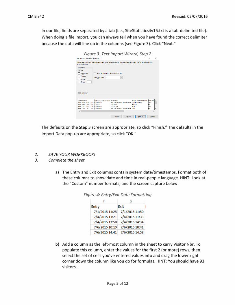
In our file, fields are separated by a tab (i.e., SiteStatistics4v15.txt is a tab-delimited file).

When doing a file import, you can always tell when you have found the correct delimiter

because the data will line up in the columns (see Figure 3). Click “Next.”

Figure 3: Text Import Wizard, Step 2

The defaults on the Step 3 screen are appropriate, so click “Finish.” The defaults in the

Import Data pop-up are appropriate, so click “OK.”

2. SAVE YOUR WORKBOOK! 3. Complete the sheet

a) The Entry and Exit columns contain system date/timestamps. Format both of these columns to show date and time in real-people language. HINT: Look at the “Custom” number formats, and the screen capture below.

Figure 4: Entry/Exit Date Formatting

b) Add a column as the left-most column in the sheet to carry Visitor Nbr. To populate this column, enter the values for the first 2 (or more) rows, then select the set of cells you’ve entered values into and drag the lower right corner down the column like you do for formulas. HINT: You should have 93 visitors.

CMIS 342 Revised: 02/07/2016

Page 6 of 12

c) Add a column to the right of the Exit column for Visit Duration. Create a formula to calculate the length of each visit to the website, and copy the formula down the Visit Duration column. Be sure to format this column as h:mm:ss (see “Custom” time formats and screen capture below).

Figure 5: Visit Duration

d) In your discussion with Mr. Allan about other description statistics you can provide for him, you determine he would like to see a few additional tables at the bottom of the sheet, specifically:

1) A summary table that provides descriptive statistics on the Visit Durations, Bandwidth, and Viewed Pages (see Figure 6). To calculate the values in the table, use the Average, Median, Max, and Min functions to reference cells in main area of the sheet. Results for Visit Duration should be in the h:mm:ss format. Results for

Bandwidth and Viewed Pages should be to 2 decimal places. (The

bandwidth in this dataset is expressed in kilobytes.)

Figure 6: Visit Summary

2) A table showing how many visitors added his site to their “Favorites” each month (see Figure 7). To do this, you want to order the data rows by month, then count the number of “Yes” occurrences in each month’s data rows. So:

i. Select the column header and data rows in the main portion of the worksheet, then use Custom Sort from the Sort & Filter dropdown from the ribbon. Sort on Entry date to get the rows grouped by month.

ii. Looking at the Entry dates, select the rows for the first month and create a range name for them (xxxFAV where xxx is an abbreviation for the month). Do this for each month

CMIS 342 Revised: 02/07/2016

Page 7 of 12

appearing in the data. NOTE: A quick way to define a range name is to use the FORMULAS tab, Define Name.

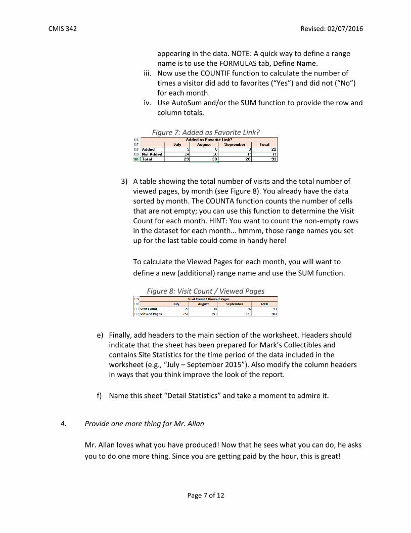
iii. Now use the COUNTIF function to calculate the number of times a visitor did add to favorites (“Yes”) and did not (“No”) for each month.

iv. Use AutoSum and/or the SUM function to provide the row and column totals.

Figure 7: Added as Favorite Link?

3) A table showing the total number of visits and the total number of viewed pages, by month (see Figure 8). You already have the data sorted by month. The COUNTA function counts the number of cells that are not empty; you can use this function to determine the Visit Count for each month. HINT: You want to count the non-empty rows in the dataset for each month… hmmm, those range names you set up for the last table could come in handy here!

To calculate the Viewed Pages for each month, you will want to

define a new (additional) range name and use the SUM function.

Figure 8: Visit Count / Viewed Pages

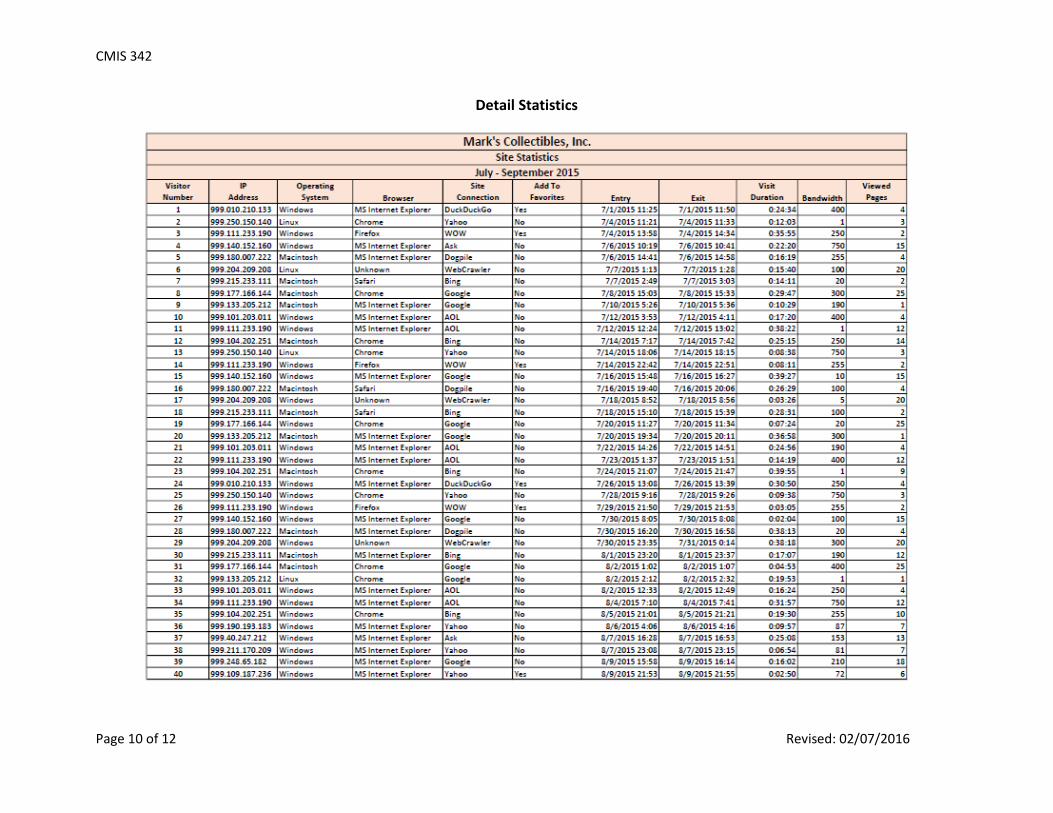
e) Finally, add headers to the main section of the worksheet. Headers should indicate that the sheet has been prepared for Mark’s Collectibles and contains Site Statistics for the time period of the data included in the worksheet (e.g., “July – September 2015”). Also modify the column headers in ways that you think improve the look of the report.

f) Name this sheet “Detail Statistics” and take a moment to admire it.

4. Provide one more thing for Mr. Allan

Mr. Allan loves what you have produced! Now that he sees what you can do, he asks

you to do one more thing. Since you are getting paid by the hour, this is great!

CMIS 342 Revised: 02/07/2016

Page 8 of 12

Mr. Allan would like charts that show the average Visit Duration by Operating

System, by Connection, and by Browser. You decide to provide these by creating 3

pivot tables/charts (one each for Operating System, Connection, and Browser). You

will place all 3 of these on the same (new) sheet in the workbook.

Here’s some guidance to help you with the first pivot table/chart:

a. Select the range of data to be used for the first pivot table (average Visit Duration by Operating System). When selecting your data for a pivot table, be sure to include the entire data area and column headers, but NOT the report headers. I find it easiest to assign a range name!

b. From the INSERT tab, in the Charts grouping, click the down arrow of PivotChart, then select PivotChart & PivotTable. For this first pivot table/chart, choose to place it in a New Worksheet.

c. Working in the Pivot Chart Fields at the right, you want Rows of this first pivot table to be Operating System.

d. Visit Duration is what you want in the data cells of your pivot table, so send it to “∑ Values”. Then click the down arrow to change Value Field Settings from Count to Average (because Mr. Allan want to see the average stay).

e. Over in the pivot table, format the Visit Duration cells to display as h:mm:ss. f. Move the chart to sit beside the table. In the chart area:

o Rename the heading of the chart as needed. o Remove the Legend.

g. Call this new sheet “Visit Duration Averages.”

Okay, you’re on your own for the other 2 pivot tables/charts! Be sure to place them

in the same sheet (your “Visit Duration Averages” sheet). HINT: After clicking the

radio button for “Existing worksheet”, go to your “Visit Duration Averages” sheet

and click in a column A cell below your prior pivot table(s).

5. At this point, your Excel file should consist of 2 worksheets named: Visit Duration Averages

Detail Statistics

Case Deliverables:

Submit your Excel file through the Blackboard assignment link. Images of how your work should

look follows.

CMIS 342 Revised: 02/07/2016

Page 9 of 12

Visit Duration Averages

CMIS 342

Page 10 of 12 Revised: 02/07/2016

Detail Statistics

CMIS 342

Page 11 of 12 Revised: 02/07/2016

CMIS 342

Page 12 of 12 Revised: 02/07/2016