excel 2007 foundation
TRANSCRIPT

8/11/2019 Excel 2007 Foundation
http://slidepdf.com/reader/full/excel-2007-foundation 1/115
Microsoft Excel 2007Foundation Level

8/11/2019 Excel 2007 Foundation
http://slidepdf.com/reader/full/excel-2007-foundation 2/115
Excel 2007 Foundation - Page 2
FOR USE AT THE LICENSED SITE(S) ONLY
Cheltenham Courseware Pty. Ltd. 1995-2008 www.cheltenhamcourseware.com
© 1995-2008 Cheltenham Courseware Pty. Ltd.
All trademarks acknowledged. E&OE.
No part of this document may be copied without written permission from Cheltenham Courseware unlessproduced under the terms of a courseware site license agreement with Cheltenham Courseware.
All reasonable precautions have been taken in the preparation of this document, including both technical andnon-technical proofing. Cheltenham Courseware and all staff assume no responsibility for any errors oromissions. No warranties are made, expressed or implied with regard to these notes. Cheltenham Coursewareshall not be responsible for any direct, incidental or consequential damages arising from the use of any materialcontained in this document. If you find any errors in these training modules, please inform CheltenhamCourseware. Whilst every effort is made to eradicate typing or technical mistakes, we apologise for any errorsyou may detect. All courses are updated on a regular basis, so your feedback is both valued by us and will helpus to maintain the highest possible standards.
Sample versions of courseware from Cheltenham Courseware(Normally supplied in Adobe Acrobat format): If the version of courseware that you are viewing is marked as NOTFOR TRAINING, SAMPLE, or similar, then it cannot be used as part of a training course, and is made availablepurely for content and style review. This is to give you the opportunity to preview our courseware, prior to makinga purchasing decision. Sample versions may not be re-sold to a third party.
For current license informationThis document may only be used under the terms of the license agreement from Cheltenham Courseware.Cheltenham Courseware reserves the right to alter the licensing conditions at any time, without prior notice.Please see the site license agreement available at: www.cheltenhamcourseware.com.au/agreement
Contact Information
Australia / Asia Pacific / Europe (ex. UK) / Rest of the World Email: [email protected] Web: www.cheltenhamcourseware.com.au
USA / Canada Email: [email protected]
Web: www.cheltenhamcourseware.com
UKEmail: [email protected] Web: www.cctglobal.com

8/11/2019 Excel 2007 Foundation
http://slidepdf.com/reader/full/excel-2007-foundation 3/115
NOT TO BE USED FOR TRAINING
Cheltenham CoursewareAffordable - Customisable - Unbeatable
• Established in 1994 with thousands of clients in over 60 countries.
• We offer you a complete library of quality, customizable and print-
on-demand computer courses inc. Windows Vista and Office 2007.
• Our training manuals are supplied in editable Microsoft Office
format.• You can edit and customise the training materials to suite your
unique training requirements.
• You can print out as many copies as you require for use at your
training site.
• There are no annual renewal fees and you can use the training
materials for as long as you like.
• No restriction on the number of people that you train at your
training site.
• The price even includes new courses developed by Cheltenham
Courseware for a whole year from your date of purchase, all for a
low, one-off fee with no annual renewal fees!
•
Generous educational and charitable discounts available (email usfor details).
• Choose the ECDL/ICDL courseware library or the IT courseware
library. Buy both and get a discount!
• Fully customisable allowing you to add your organisation’s name
and logos to the training manuals.
• Includes training manuals, exercise files, slides and more!
• Choose from Standard or Professional editions to suit your
requirements. Intranet versions available within the Professional
Edition Courseware.
• Sample downloads available for all our courses, including
Windows, Microsoft Office and many more.
• Suitable for tutor-led training, self teach, post-course reference or
as part of a blended learning approach.
Clients cover corporates, governments,
schools, colleges, universities and
commercial training companies including
such well known organisations as Canon,
IBM, Lloyds, Hertz, Royal Mail, Medical
Research Council, NHS Executive South
and West, Oxford University, Pen State
University, University of Cambridge,
University of Florida, UK Passport
Service, US House of Representatives,
the British Embassy in Washington and
the London Fire Brigade.
If you like this sample,
please show it to your
training department.
We provide the training manuals so you can concentrate on the training delivery.
Purchase your IT courseware from a company that has a proven track record.

8/11/2019 Excel 2007 Foundation
http://slidepdf.com/reader/full/excel-2007-foundation 4/115
1995-2007 Cheltenham Courseware Pty. Ltd. Phone: 1300 852 204 Fax: 1300 852 206Email: [email protected] Internet: http://www. cheltenhamcourseware.com.au
Questions to ask our competitors• Do they supply a library of training courses, at a price even remotely close to our low prices?
• Are complete samples of ALL the IT courses available for download so that you can judge the quality?
• If they offer courses on a site license basis, is the full range of courses are included?
• Is the site license an annual license or a one-off payment?• Are the training materials fully editable and can you add your own name and logos?
• Are the manuals easy to edit using standard 'cut and paste' techniques and can the table of contents
be easily updated, or do I have to use proprietary software to edit the materials?
• Are upgrades and new courses included free of charge for 12 months?
• Are Intranet versions available?
• Are PowerPoint slides included in the price?
If you are unhappy with your current computer courseware supplier, please download our samples
now and switch to our quality driven, cost effective courseware solution.
Our commitment to ECDL / ICDL• The European Computer Driving Licence® (ECDL) is the internationally recognised qualification which
enables people to demonstrate their competence in computer skills. The record breaking ECDL / ICDL
certification is the fastest growing IT user qualification in over 125 countries.
• Our ECDL / ICDL training manuals are approved for the UK, Ireland, Australia, Cyprus, Middle East
(UNESCO region), South Africa and the Asia Pacific region.
• Cheltenham Courseware was first courseware company to release ECDL courseware.
• We were first company to release ECDL Foundation approved Advanced Level courseware.
• We were one of the first companies in the world to release courseware for ECDL syllabus 4.
• We worked with the United Nations (UNESCO) to produce the first Arabic ICDL courseware.
• We were one of the first companies in to release approved courseware for ECDL/ICDL WebStarter
Contact Details:
UK/Ireland: www.cctglobal.comUSA/Canada: www.cheltenhamcourseware.com Australia/Rest of the world: www.cheltenhamcourseware.com.au
8/11/2019 Excel 2007 Foundation
http://slidepdf.com/reader/full/excel-2007-foundation 5/115
Excel 2007 Foundation - Page 3
FOR USE AT THE LICENSED SITE(S) ONLY
Cheltenham Courseware Pty. Ltd. 1995-2008 www.cheltenhamcourseware.com
A FIRST LOOK AT EXCEL ................................................................................................................................ 6
Starting the Excel program ....................................................................................................................... 6
What is the Active Cell?............................................................................................................................. 6
The Excel cell referencing system ........................................................................................................... 7
Entering numbers and text ........................................................................................................................ 7
Default text and number alignment .......................................................................................................... 8
Summing a column of numbers ............................................................................................................... 8
Worksheets and Workbooks ..................................................................................................................... 9
Saving a workbook ................................................................................................................................... 10
Closing a workbook .................................................................................................................................. 11
Creating a new workbook ........................................................................................................................ 12
Opening a workbook ................................................................................................................................ 12
Switching between workbooks ............................................................................................................... 12
Saving a workbook using another name ............................................................................................... 13
Saving a workbook using a different file type ....................................................................................... 13
HELP .................................................................................................................................................................... 14
Getting help ............................................................................................................................................... 14
Searching for Help .................................................................................................................................... 17
The Help 'Table of Contents' .................................................................................................................. 18
Printing a Help topic ................................................................................................................................. 19
Alt key help ................................................................................................................................................ 19
USING EXCEL ................................................................................................................................................... 21
SELECTION TECHNIQUES ................................................................................................................................. 21
Why are selection techniques important? ............................................................................................. 21
Selecting a cell .......................................................................................................................................... 21
Selecting a range of connecting cells .................................................................................................... 21
Selecting a range of non-connecting cells ............................................................................................ 21 Selecting the entire worksheet ............................................................................................................... 22
Selecting a row ......................................................................................................................................... 22
Selecting a range of connecting rows ................................................................................................... 22
Selecting a range of non-connected rows ............................................................................................ 23
Selecting a column ................................................................................................................................... 23
Selecting a range of connecting columns ............................................................................................. 23
Selecting a range of non-connecting columns ..................................................................................... 24
M ANIPULATING ROWS AND COLUMNS .............................................................................................................. 24
Inserting rows into a worksheet .............................................................................................................. 24
Inserting columns into a worksheet ....................................................................................................... 25
Deleting rows within a worksheet ........................................................................................................... 26
Deleting columns within a worksheet .................................................................................................... 27 Modifying column widths ......................................................................................................................... 27
Modifying column widths using 'drag and drop' ................................................................................... 27
Automatically resizing the column width to fit contents ...................................................................... 28
Modifying row heights .............................................................................................................................. 28
COPYING, MOVING AND DELETING .................................................................................................................. 29
Copying the cell or range contents ........................................................................................................ 29
Deleting cell contents ............................................................................................................................... 30
Moving the contents of a cell or range .................................................................................................. 31
Editing cell content ................................................................................................................................... 31
Undo and Redo ......................................................................................................................................... 31
AutoFill ....................................................................................................................................................... 32
Sorting a cell range .................................................................................................................................. 32
Searching and replacing data ................................................................................................................. 34

8/11/2019 Excel 2007 Foundation
http://slidepdf.com/reader/full/excel-2007-foundation 6/115
Excel 2007 Foundation - Page 4
FOR USE AT THE LICENSED SITE(S) ONLY
Cheltenham Courseware Pty. Ltd. 1995-2008 www.cheltenhamcourseware.com
WORKSHEETS .................................................................................................................................................. 36
M ANIPULATING WORKSHEETS......................................................................................................................... 36
Switching between worksheets .............................................................................................................. 36
Renaming a worksheet ............................................................................................................................ 36
Inserting a new worksheet ...................................................................................................................... 36
Deleting a worksheet ............................................................................................................................... 37
Copying a worksheet within a workbook ............................................................................................... 38
Moving a worksheet within a workbook ................................................................................................ 39
Copying or moving worksheets between workbooks .......................................................................... 40
FORMATTING .................................................................................................................................................... 43
FONT FORMATTING .......................................................................................................................................... 43
Font type .................................................................................................................................................... 43
Font size .................................................................................................................................................... 44
Bold, italic, underline formatting ............................................................................................................. 44
Cell border formatting .............................................................................................................................. 45
Formatting the background colour ......................................................................................................... 46
Formatting the font colour ....................................................................................................................... 46
ALIGNMENT FORMATTING ................................................................................................................................ 47
Aligning contents in a cell range ............................................................................................................ 47
Centring a title over a cell range ............................................................................................................ 47
Cell orientation .......................................................................................................................................... 48
Text wrapping ........................................................................................................................................... 48
Format painter ........................................................................................................................................... 49
NUMBER FORMATTING ..................................................................................................................................... 49
Number formatting .................................................................................................................................... 50
Decimal point display ............................................................................................................................... 50
Comma formatting .................................................................................................................................... 51
Currency symbol ....................................................................................................................................... 51
Date styles ................................................................................................................................................. 51
Percentages .............................................................................................................................................. 53
FREEZING ROW AND COLUMN TITLES .............................................................................................................. 53
Freezing row and column titles ............................................................................................................... 53
FORMULAS AND FUNCTIONS ...................................................................................................................... 56
FORMULAS ....................................................................................................................................................... 56
Creating formulas ..................................................................................................................................... 56
Easy way to create formulas ................................................................................................................... 56
Copying formulas ...................................................................................................................................... 57
Operators ................................................................................................................................................... 58
Formula error messages ......................................................................................................................... 58
RELATIVE, MIXED AND ABSOLUTE CELL REFERENCING ................................................................................... 59
Relative cell referencing within formulas............................................................................................... 59
Absolute cell referencing within formulas ............................................................................................. 59
FUNCTIONS ...................................................................................................................................................... 61
What is a function? ................................................................................................................................... 61
Common functions ................................................................................................................................... 61
Sum function ............................................................................................................................................. 62
Average function ....................................................................................................................................... 64
Max function .............................................................................................................................................. 66
Min function ............................................................................................................................................... 67
Count function ........................................................................................................................................... 69
What are 'IF functions'? ........................................................................................................................... 72
Using the IF function ................................................................................................................................ 72
CHARTS .............................................................................................................................................................. 76

8/11/2019 Excel 2007 Foundation
http://slidepdf.com/reader/full/excel-2007-foundation 7/115
Excel 2007 Foundation - Page 5
FOR USE AT THE LICENSED SITE(S) ONLY
Cheltenham Courseware Pty. Ltd. 1995-2008 www.cheltenhamcourseware.com
USING CHARTS ................................................................................................................................................ 76
Inserting a column chart .......................................................................................................................... 76
Inserting a line chart ................................................................................................................................. 77
Inserting a bar chart ................................................................................................................................. 78
Inserting a pie chart .................................................................................................................................. 79
Resizing a chart ........................................................................................................................................ 79
Deleting a chart ......................................................................................................................................... 79
Chart title or labels ................................................................................................................................... 79
Chart background colour ......................................................................................................................... 82
Changing the column, bar, line or pie slice colours in a chart ........................................................... 84
Changing the chart type .......................................................................................................................... 87
Modifying Charts using the Layout tab .................................................................................................. 88
Copying and moving charts within a worksheet ................................................................................... 91
Copying and moving charts between worksheets ............................................................................... 92
Copying and moving charts between workbooks ................................................................................ 92
CUSTOMIZING EXCEL .................................................................................................................................... 93
Modifying basic options ........................................................................................................................... 93
Minimising the Ribbon ............................................................................................................................. 95 AutoCorrect options ................................................................................................................................. 96
PRINTING ........................................................................................................................................................... 98
WORKSHEET SETUP ........................................................................................................................................ 98
Worksheet margins .................................................................................................................................. 98
Worksheet orientation .............................................................................................................................. 99
Worksheet page size ............................................................................................................................. 100
Headers and Footers ............................................................................................................................. 100
Header and footer fields ........................................................................................................................ 102
Scaling your worksheet to fit a page(s) ............................................................................................... 102
PREPARING TO PRINT A WORKSHEET ............................................................................................................ 104
Visually check your calculations ........................................................................................................... 104 Gridline display when printing ............................................................................................................... 105
Printing titles on every page when printing ......................................................................................... 106
Printing the Excel row and column headings ..................................................................................... 109
Spell checking ......................................................................................................................................... 109
Previewing a worksheet ......................................................................................................................... 110
Comparing Workbooks side by side .................................................................................................... 110
Zooming the view ................................................................................................................................... 110
Printing options ....................................................................................................................................... 111

8/11/2019 Excel 2007 Foundation
http://slidepdf.com/reader/full/excel-2007-foundation 8/115
Excel 2007 Foundation - Page 6
FOR USE AT THE LICENSED SITE(S) ONLY
Cheltenham Courseware Pty. Ltd. 1995-2008 www.cheltenhamcourseware.com
A first look at Excel
Starting the Excel program
• Click on the Start button (bottom-left of the screen). Click on All Programs.Click on Microsoft Office. Click on Microsoft Office Excel 2007. TheExcel window will be displayed, as illustrated.
What is the Active Cell?
• Excel identifies the active cell with a bold outline around the cell andhighlighting the column heading letter and row heading number of the cell.In the following example, B2 is the active cell:
• In the above illustration, notice that B2 is displayed in the Name Box, andthe contents of the cell is displayed in the Formula Bar. In this case, 2002
is a calculated value, 2000+2.
• In order for you to enter data into a cell, it needs to be the active cell. The
active cell will accept keyboard entries. You can make a cell active byclicking on it or navigating to it.

8/11/2019 Excel 2007 Foundation
http://slidepdf.com/reader/full/excel-2007-foundation 9/115
Excel 2007 Foundation - Page 7
FOR USE AT THE LICENSED SITE(S) ONLY
Cheltenham Courseware Pty. Ltd. 1995-2008 www.cheltenhamcourseware.com
The Excel cell referencing system
• An Excel worksheet is made up of individual cells, each of which had a uniquereference. Look at the illustration below. We have clicked on cell B3, which
means that the cell is in column B, row 3.
In the illustration below, we have clicked on cell D2.
If you look carefully you will see that the current cell reference is displayed
just above the actual worksheet.
Entering numbers and text
• Click on cell B2, as illustrated.
• Type in the word 'Region'. Press the Enter key. When you press the Enter key you will automatically drop down to the next cell within the worksheet.Your screen will now look like this.
• The active cell is now B3. Type in the word 'North'. Press the Enter key.
• The active cell is now B4. Type in the word 'South'. Press the Enter key.

8/11/2019 Excel 2007 Foundation
http://slidepdf.com/reader/full/excel-2007-foundation 10/115
Excel 2007 Foundation - Page 8
FOR USE AT THE LICENSED SITE(S) ONLY
Cheltenham Courseware Pty. Ltd. 1995-2008 www.cheltenhamcourseware.com
• The active cell is now B5. Type in the word 'East'. Press the Enter key.
• The active cell is now B6. Type in the word 'West'. Press the Enter key.
Your screen will now look like this:
• Click on cell C2. Type in the word 'Sales'. Press the Enter key.
• Type in the number 10488 and press the Enter key.• Type in the number 11973 and press the Enter key.
• Type in the number 13841 and press the Enter key.
• Type in the number 16284 and press the Enter key.
Your screen will now look like this:
Default text and number alignment
• If you look carefully at what you have typed in you will see that by defaulttext is aligned within a cell to the left, while numbers are aligned within thecell to the right. This makes sense, as normally text starts from the left of a
page and it is the same within a cell. Numbers on the other hand normallyalign to the right. Think how you would write down a column of numbers ona page that you want to add up. Numbers align to the right.
Summing a column of numbers
• Click on cell B7 and type in the word 'Total'.
• Click on cell C7. Click on the Formulas tab, and then click on the AutoSum
button.

8/11/2019 Excel 2007 Foundation
http://slidepdf.com/reader/full/excel-2007-foundation 11/115
Excel 2007 Foundation - Page 9
FOR USE AT THE LICENSED SITE(S) ONLY
Cheltenham Courseware Pty. Ltd. 1995-2008 www.cheltenhamcourseware.com
Your screen will look like this:
• Press the Enter key and Excel will automatically add up the column ofnumbers, as illustrated.
• We have hardly started to use Excel but already you have seen how powerfuland easy to use it is. We will see more of the Excel functions for performingcalculations later.
The best thing about Excel is that if you make changes to the numbers then
totals and other calculations are automatically updated. Click on cell C4 andtype in a different number. When you press the Enter key you will see thatthe total value displayed in cell C7 changes to recalculate the total vales of
the sales.
Worksheets and Workbooks
• Look at the bottom-left of your screen and you will see the worksheet tabs
displayed.

8/11/2019 Excel 2007 Foundation
http://slidepdf.com/reader/full/excel-2007-foundation 12/115
Excel 2007 Foundation - Page 10
FOR USE AT THE LICENSED SITE(S) ONLY
Cheltenham Courseware Pty. Ltd. 1995-2008 www.cheltenhamcourseware.com
By default each workbook contains three worksheets. This is similar to a
notebook that contains separate pages. Click on the Sheet 2 worksheet taband the second worksheet is displayed. Click on the Sheet 3 worksheet taband the third worksheet is displayed. Click on the Sheet 1 worksheet tab
and the first worksheet, containing your data is displayed again. As we willsee later you can add or remove worksheets as well as reordering and
renaming them.
Saving a workbook
• To save the workbook click on the Save icon (top-left part of your screen).
This will display the Save As dialog box.
• Click on the down arrow next to the Save in section of the dialog box tonavigate to the folder containing your sample files.
• Click within the File name section of the dialog box to name the file. In this
case use the file name My First Spreadsheet.

8/11/2019 Excel 2007 Foundation
http://slidepdf.com/reader/full/excel-2007-foundation 13/115
Excel 2007 Foundation - Page 11
FOR USE AT THE LICENSED SITE(S) ONLY
Cheltenham Courseware Pty. Ltd. 1995-2008 www.cheltenhamcourseware.com
• Click on the Save button the save the file to disk.
Closing a workbook
• To close the workbook, click on the Microsoft Office Button (top-left of
your screen), from the drop down options displayed, click on the Close command.
• The screen will now look like the illustration below. The Excel program isopen but no workbook is displayed within the program.
8/11/2019 Excel 2007 Foundation
http://slidepdf.com/reader/full/excel-2007-foundation 14/115
Excel 2007 Foundation - Page 12
FOR USE AT THE LICENSED SITE(S) ONLY
Cheltenham Courseware Pty. Ltd. 1995-2008 www.cheltenhamcourseware.com
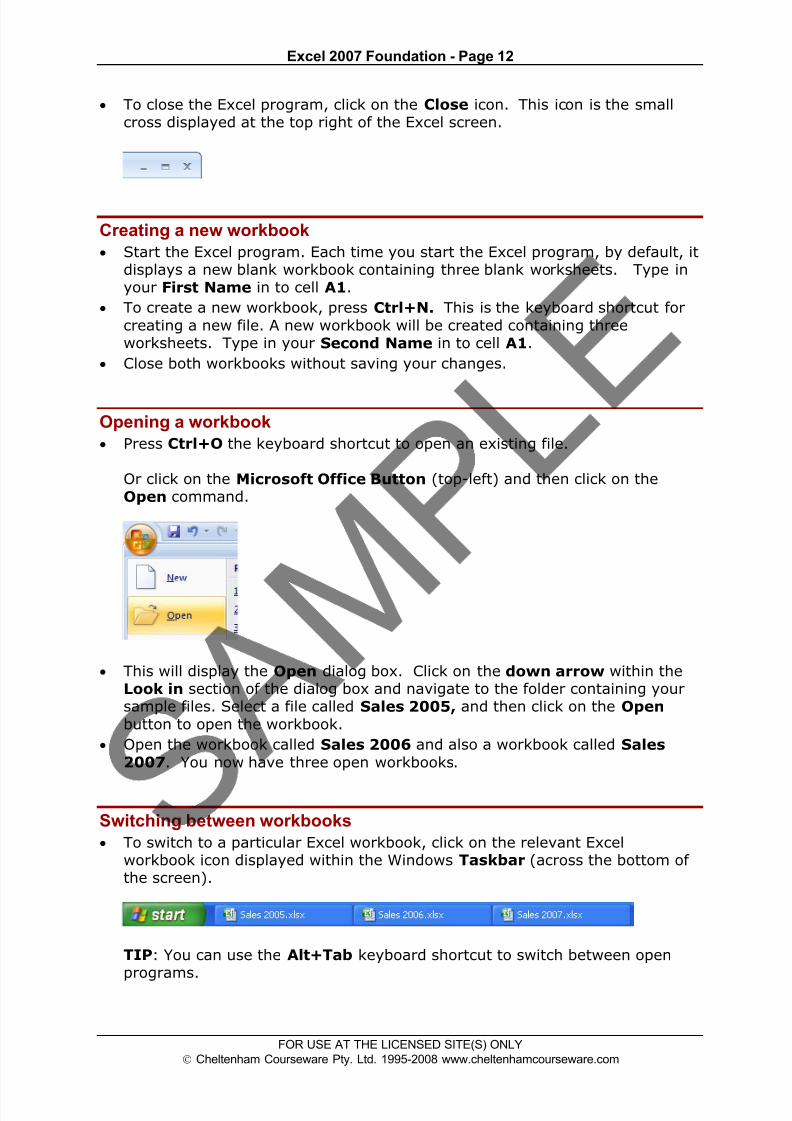
• To close the Excel program, click on the Close icon. This icon is the smallcross displayed at the top right of the Excel screen.
Creating a new workbook
• Start the Excel program. Each time you start the Excel program, by default, itdisplays a new blank workbook containing three blank worksheets. Type inyour First Name in to cell A1.
• To create a new workbook, press Ctrl+N. This is the keyboard shortcut for
creating a new file. A new workbook will be created containing threeworksheets. Type in your Second Name in to cell A1.
• Close both workbooks without saving your changes.
Opening a workbook
• Press Ctrl+O the keyboard shortcut to open an existing file.
Or click on the Microsoft Office Button (top-left) and then click on the
Open command.
• This will display the Open dialog box. Click on the down arrow within the
Look in section of the dialog box and navigate to the folder containing yoursample files. Select a file called Sales 2005, and then click on the Open
button to open the workbook.
• Open the workbook called Sales 2006 and also a workbook called Sales2007. You now have three open workbooks.
Switching between workbooks
• To switch to a particular Excel workbook, click on the relevant Excelworkbook icon displayed within the Windows Taskbar (across the bottom ofthe screen).
TIP: You can use the Alt+Tab keyboard shortcut to switch between openprograms.

8/11/2019 Excel 2007 Foundation
http://slidepdf.com/reader/full/excel-2007-foundation 15/115
Excel 2007 Foundation - Page 13
FOR USE AT THE LICENSED SITE(S) ONLY
Cheltenham Courseware Pty. Ltd. 1995-2008 www.cheltenhamcourseware.com
• Close all open workbooks.
Saving a workbook using another name
• Open the workbook called Sales 2005. Click on the Microsoft OfficeButton and the select the Save As command.
• In the File name section enter a new file name, in this case called MyBackup. Click on the Save button. You now have two copies of the samefile, both containing the same information. This can be useful for making
backups of your data or for retaining copies of a workbook with different
versions of the data in each file.
Saving a workbook using a different file type
• Click on the Microsoft Office Button and the select the Save As command.The Save As dialog is displayed. Click on the down arrow within the Saveas type section of the dialog box. You can select the required file type fromthe drop down displayed.
TIP: If you want to email a copy of an Excel 2007 workbook to someone that
has an earlier version of Excel, such as Excel 2003, then you may need tosave the file in the Excel 97-2003 Workbook file format.
Alternatively, people with earlier versions of Excel can download additional
free software from Microsoft allowing them to open and view (but notnecessary edit), files created using Excel 2007.
• Close any open dialog boxes and close all open worksheets.

8/11/2019 Excel 2007 Foundation
http://slidepdf.com/reader/full/excel-2007-foundation 16/115
Excel 2007 Foundation - Page 14
FOR USE AT THE LICENSED SITE(S) ONLY
Cheltenham Courseware Pty. Ltd. 1995-2008 www.cheltenhamcourseware.com
Help
Getting help
• Click on the Microsoft Office Excel Help icon (towards the top-right of thescreen).
TIP: Or press the F1 help key.
• The Excel Help window is displayed.
• As you can see a wide range of help topics are displayed. Click on the
What's new link. You will see the following.

8/11/2019 Excel 2007 Foundation
http://slidepdf.com/reader/full/excel-2007-foundation 17/115
Excel 2007 Foundation - Page 15
FOR USE AT THE LICENSED SITE(S) ONLY
Cheltenham Courseware Pty. Ltd. 1995-2008 www.cheltenhamcourseware.com
• Click on the What's new in Microsoft Office Excel 2007 link. You will seethe following.

8/11/2019 Excel 2007 Foundation
http://slidepdf.com/reader/full/excel-2007-foundation 18/115
Excel 2007 Foundation - Page 16
FOR USE AT THE LICENSED SITE(S) ONLY
Cheltenham Courseware Pty. Ltd. 1995-2008 www.cheltenhamcourseware.com
TIP: Click on the Maximise button within the top-right part of the dialogbox. This will make the dialog box fill the screen and the information within itwill be easier to read.
• Spend a little time browsing what's new within this version of Excel. Forinstance if you click on the Results Orientated User Interface link you will
see the following.

8/11/2019 Excel 2007 Foundation
http://slidepdf.com/reader/full/excel-2007-foundation 19/115
Excel 2007 Foundation - Page 17
FOR USE AT THE LICENSED SITE(S) ONLY
Cheltenham Courseware Pty. Ltd. 1995-2008 www.cheltenhamcourseware.com
• When you have finished experimenting, close the Excel Help window.
Searching for Help
• You can search for help on a topic of particular interest. Press F1 to displaythe Excel Help window. Within the text box near the top of the Excel Helpwindow, type in a word or words relating to the help you need. For instance,
to display help about printing, type in the word 'printing'
• Click on the Search button next to the text input box. You will see a range
of topics related to printing. Clicking on any of these topics will display moreinformation about printing.

8/11/2019 Excel 2007 Foundation
http://slidepdf.com/reader/full/excel-2007-foundation 20/115
Excel 2007 Foundation - Page 18
FOR USE AT THE LICENSED SITE(S) ONLY
Cheltenham Courseware Pty. Ltd. 1995-2008 www.cheltenhamcourseware.com
• Close the Excel Help window when you have finished experimenting.
The Help 'Table of Contents'
• Press F1 to display the Excel Help window. Click on the Table of Contents icon (the book icon displayed within the Excel Help window toolbar).
• You will now see a Table of Contents displayed down the left side of the Excel
Help window.

8/11/2019 Excel 2007 Foundation
http://slidepdf.com/reader/full/excel-2007-foundation 21/115
Excel 2007 Foundation - Page 19
FOR USE AT THE LICENSED SITE(S) ONLY
Cheltenham Courseware Pty. Ltd. 1995-2008 www.cheltenhamcourseware.com
Printing a Help topic• Display an item of interest within the Excel Help window. Click on the Print
icon displayed within the Excel Help toolbar.
• Close all open dialog boxes before continuing.
Alt key help
• Press CTRL+N to open a new blank workbook
• Click on the Home tab.
• Press the Alt key and you will see numbers and letters displayed over icons,tabs or commands, towards the top of your screen.
8/11/2019 Excel 2007 Foundation
http://slidepdf.com/reader/full/excel-2007-foundation 22/115
Excel 2007 Foundation - Page 20
FOR USE AT THE LICENSED SITE(S) ONLY
Cheltenham Courseware Pty. Ltd. 1995-2008 www.cheltenhamcourseware.com
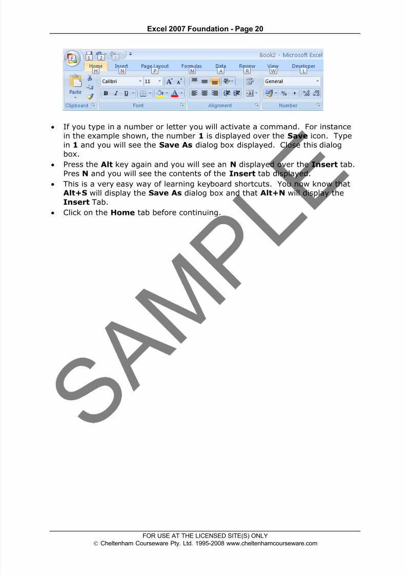
• If you type in a number or letter you will activate a command. For instancein the example shown, the number 1 is displayed over the Save icon. Type
in 1 and you will see the Save As dialog box displayed. Close this dialogbox.
• Press the Alt key again and you will see an N displayed over the Insert tab.
Pres N and you will see the contents of the Insert tab displayed.
• This is a very easy way of learning keyboard shortcuts. You now know thatAlt+S will display the Save As dialog box and that Alt+N will display the
Insert Tab.• Click on the Home tab before continuing.

8/11/2019 Excel 2007 Foundation
http://slidepdf.com/reader/full/excel-2007-foundation 23/115
Excel 2007 Foundation - Page 21
FOR USE AT THE LICENSED SITE(S) ONLY
Cheltenham Courseware Pty. Ltd. 1995-2008 www.cheltenhamcourseware.com
Using Excel
Selection techniques
Why are selection techniques important?
• Often when you want to do something within Excel you need to select anitem first. This could involve selecting a cell or multiple cells. It many needyou to select a row, a column or even the entire table.
Selecting a cell
• Open a workbook called Selection techniques. To select a cell simply click
on that cell. Thus to select cell B3, click on cell B3.
Selecting a range of connecting cells
• We want to select the cells from C3 to G3. To do this click on the first cellwithin the range, i.e. C3. Then press down the Shift key (and keep it helddown). Click on cell G3. When you release the Shift key the cell range willremain selected, as illustrated.
Selecting a range of non-connecting cells
• Sometimes we need to select multiple cells that are not next to each other,as in the example below, where C3, E3 and G3 have been selected.
To do this click on the first cell, i.e. C3. Then while keeping the Ctrl keypressed click on the cells E3 and G3. When you release the Ctrl key the
cells will remain selected.

8/11/2019 Excel 2007 Foundation
http://slidepdf.com/reader/full/excel-2007-foundation 24/115
Excel 2007 Foundation - Page 22
FOR USE AT THE LICENSED SITE(S) ONLY
Cheltenham Courseware Pty. Ltd. 1995-2008 www.cheltenhamcourseware.com
Selecting the entire worksheet
• To select the entire worksheet, click on the intersection between the columnand row referencing numbers.
Selecting a row
• To select a row, say the row relating to Canada, click on the relevant rownumber displayed down the left side of the worksheet.
Selecting a range of connecting rows
• To select the rows relating to Canada, USA, UK and Australia. First click onthe row number next to Canada (i.e. 5). Press down the Shift key and keep
it pressed. Click on the row number relating to Australia (i.e. 8). When yourelease the Shift key the multiple rows remain selected.

8/11/2019 Excel 2007 Foundation
http://slidepdf.com/reader/full/excel-2007-foundation 25/115
Excel 2007 Foundation - Page 23
FOR USE AT THE LICENSED SITE(S) ONLY
Cheltenham Courseware Pty. Ltd. 1995-2008 www.cheltenhamcourseware.com
Selecting a range of non-connected rows
• Click on the row number 3 and press down the Ctrl key. Click on rownumber 5, then row number 7 and finally number 9. Release the Ctrl key
and the rows will remain selected.
Selecting a column
• To select the column containing data relating to 2003, click on the columnheader C, as illustrated.
Selecting a range of connecting columns
• To select the columns relating to the sales figures for 2003-2006, first selectcolumn C. Press the Shift key and while keeping it pressed select column F.When you release the Shift key the columns will remain selected.

8/11/2019 Excel 2007 Foundation
http://slidepdf.com/reader/full/excel-2007-foundation 26/115
Excel 2007 Foundation - Page 24
FOR USE AT THE LICENSED SITE(S) ONLY
Cheltenham Courseware Pty. Ltd. 1995-2008 www.cheltenhamcourseware.com
Selecting a range of non-connecting columns
• To select the columns relating to 2003, 2005 and 2005, first select thecolumn C. Press the Ctrl key and keep it pressed. Select column E and thenselect column G. Release the Ctrl key and the columns remain selected.
• Close the workbook without saving any changes you may have made.
Manipulating rows and columns
Inserting rows into a worksheet
• Open a workbook called Rows and columns.
• We need to insert a row for Japan between the row for Canada and the rowfor the USA. Select the row for the USA, as illustrated.

8/11/2019 Excel 2007 Foundation
http://slidepdf.com/reader/full/excel-2007-foundation 27/115
Excel 2007 Foundation - Page 25
FOR USE AT THE LICENSED SITE(S) ONLY
Cheltenham Courseware Pty. Ltd. 1995-2008 www.cheltenhamcourseware.com
• Right click over the selected row and from the popup menu displayed selectthe Insert command.
• The table will now look like this.
• Click on cell B6 and type in the word 'Japan'. Enter the following sales
figures for Japan.
Inserting columns into a worksheet
• We want to insert a column for sales figures in 2002, which needs to beinserted before the 2003 column. Select the column relating to 2003, asillustrated.

8/11/2019 Excel 2007 Foundation
http://slidepdf.com/reader/full/excel-2007-foundation 28/115
Excel 2007 Foundation - Page 26
FOR USE AT THE LICENSED SITE(S) ONLY
Cheltenham Courseware Pty. Ltd. 1995-2008 www.cheltenhamcourseware.com
• Right click over the selected column and from the popup menu displayedselect the Insert command. The column will be inserted, as illustrated.
• Enter the following data into the column.
Deleting rows within a worksheet
• Select the row relating to Canada. Right click over the selected row and fromthe popup menu displayed select the Delete command.
• The row is deleted without any additional warning.
TIP: To delete multiple connected rows, just the Shift key trick to selectmultiple rows and then right click to delete the rows. To delete multiple non-connected rows, use the Ctrl key trick to select the multiple rows and then
right click to delete the rows.

8/11/2019 Excel 2007 Foundation
http://slidepdf.com/reader/full/excel-2007-foundation 29/115
Excel 2007 Foundation - Page 27
FOR USE AT THE LICENSED SITE(S) ONLY
Cheltenham Courseware Pty. Ltd. 1995-2008 www.cheltenhamcourseware.com
Deleting columns within a worksheet
• Select the column relating to Sales 2007. Right click over the selectedcolumn and from the popup menu displayed select the Delete command.
The column is deleted without any additional warning.
TIP: To delete multiple connected columns, use the Shift key trick to selectmultiple columns and then right click to delete the columns. To delete
multiple non-connected columns, use the Ctrl key trick to select the multiplecolumns and then right click to delete the columns.
Modifying column widths
• Select a column, such as the Country column. Right click over the selectedcolumn and from the popup menu displayed select the Column Width
command.
• The Column Width dialog box is displayed which allows you to set thecolumn width. Click on the Cancel button to close the dialog box.
Modifying column widths using 'drag and drop'
• Move the mouse pointer to the line between the header for column B andcolumn C, as illustrated below.

8/11/2019 Excel 2007 Foundation
http://slidepdf.com/reader/full/excel-2007-foundation 30/115
Excel 2007 Foundation - Page 28
FOR USE AT THE LICENSED SITE(S) ONLY
Cheltenham Courseware Pty. Ltd. 1995-2008 www.cheltenhamcourseware.com
• Press the mouse button and keep it pressed. Move the mouse pointer left or
right to make the column narrower or wider. Release the mouse button and
the column width will change as required.
Automatically resizing the column width to fit contents
• Resize all the columns so that they are too narrow to properly display thedata contained within the columns. Your screen will look similar that the
illustration below.
• To automatically resize each column width to fit the contents, select all thecolumns containing data. Double click on the junction between one of the
column header headers within the selected columns.
Modifying row heights• Select one or more rows and then right click over the selected row(s). From
the popup menu displayed select the Row Height command.

8/11/2019 Excel 2007 Foundation
http://slidepdf.com/reader/full/excel-2007-foundation 31/115
Excel 2007 Foundation - Page 29
FOR USE AT THE LICENSED SITE(S) ONLY
Cheltenham Courseware Pty. Ltd. 1995-2008 www.cheltenhamcourseware.com
• The Row Height dialog is displayed allowing you to set the exact row height,
as required.
TIP: If you click between any two row headers, you can drag the row heightup or down as required, to modify the row height.
• Save your changes and close the workbook.
Copying, Moving and Deleting
Copying the cell or range contents
• Open a workbook called Copying moving and deleting.
• Select a cell, range, row or column to copy. In this case select the range B4
to E4.
TIP: A range like this is often written as B4:E4.
Your screen will look something like this:

8/11/2019 Excel 2007 Foundation
http://slidepdf.com/reader/full/excel-2007-foundation 32/115
Excel 2007 Foundation - Page 30
FOR USE AT THE LICENSED SITE(S) ONLY
Cheltenham Courseware Pty. Ltd. 1995-2008 www.cheltenhamcourseware.com
• Press Ctrl+C to copy the selected range to the Clipboard.
TIP: To copy a selected item to the Clipboard, click on the Home tab andthen click on the Copy icon in the Clipboard group on the Ribbon.
• Click at the location you wish to paste the data to. In this case click on cell
B14 and press the Ctrl+V keys to paste the data from the Clipboard.
TIP: To copy a selected item to the Clipboard, click on the Home tab andthen click on the Paste icon, in the Clipboard group on the Ribbon.
• Your data will now look like this.
TIP: You can use the same technique to copy entire rows or columns.Pressing Ctrl+A will select everything within a worksheet and allow you to
copy the entire worksheet contents to the Clipboard when you press Ctrl+C.
Deleting cell contents
• Select the range that you wish to delete the contents of. In this case selectthe range B10:E10, as illustrated.

8/11/2019 Excel 2007 Foundation
http://slidepdf.com/reader/full/excel-2007-foundation 33/115
Excel 2007 Foundation - Page 31
FOR USE AT THE LICENSED SITE(S) ONLY
Cheltenham Courseware Pty. Ltd. 1995-2008 www.cheltenhamcourseware.com
• Press the Del key and the cell contents will be deleted.
TIP: You can use the same technique to delete entire rows or columns.Pressing Ctrl+A will select everything within a worksheet will allow you to
delete the entire worksheet contents when you press the Del key.
Moving the contents of a cell or range
• Select the range to wish to move and then cut it to the Clipboard. In thiscase select the data, as illustrated.
• Press the Ctrl+X keys to cut the selected data to the Clipboard.Click at the location you wish to move the selected data to, in this case click
in cell B15, and press Ctrl+V, to paste the data.
TIP: You can use the same technique to move entire rows or columns.
• Save your changes and close the workbook.
Editing cell content
• It is easy to edit existing data within a cell or to replace existing data within acell. Open a workbook called Editing.
• Click on cell B3. Double click in front of the word 'Region' and insert the
word 'Sales' followed by a space.
• Click on cell B7. Double click on the word 'West', to select it and then overtype the selected word with the word 'Central'.
Undo and Redo
• Click on the Undo icon (top-left of your screen) to reverse the last action.Try it now.

8/11/2019 Excel 2007 Foundation
http://slidepdf.com/reader/full/excel-2007-foundation 34/115
Excel 2007 Foundation - Page 32
FOR USE AT THE LICENSED SITE(S) ONLY
Cheltenham Courseware Pty. Ltd. 1995-2008 www.cheltenhamcourseware.com
• Click on the Redo icon (top-left of your screen) to reapply the last action.Try it now.
• Save your changes and close the workbook.
AutoFill
• Open a workbook called AutoFill.
• Click on cell B3 which contains the word Monday. Move the mouse pointer tothe bottom-right corner of this cell and the mouse pointer shape will changeto the shape of a small black cross. When the mouse pointer changes shape,
press the mouse button down, and while keeping it pressed move slowly
down the page. When you release the mouse button you will see that Excelhas 'AutoFilled' the range you dragged across with days of the week.
• Click on cell C3 which contains the word January. Use the AutoFill feature to
automatically create a column containing all the months of the year.
• Select the cell range D3:D4. Use AutoFill to extend the series down thepage. As you will see the series becomes 1,2,3,4,5,6,7 etc.
• Select the cell range E3:E4. Use AutoFill to extend the series down the
page. As you will see the series becomes 2,4,6,8,10 etc.
• Save your changes and close the workbook.
Sorting a cell range
• Open a workbook called Sorting.• Click within the data contained within column B.
• Click on the Data tab and from within the Sort & Filter group, click on SortA to Z icon.
The data will be displayed as illustrated.

8/11/2019 Excel 2007 Foundation
http://slidepdf.com/reader/full/excel-2007-foundation 35/115
Excel 2007 Foundation - Page 33
FOR USE AT THE LICENSED SITE(S) ONLY
Cheltenham Courseware Pty. Ltd. 1995-2008 www.cheltenhamcourseware.com
• Click on the Sort Z to A icon.
The data will be displayed as illustrated.
• Click within the data contained in column C.• Click on the Data tab, and from within the Sort & Filter group, click on Sort
A to Z icon.
The data will be displayed as illustrated.

8/11/2019 Excel 2007 Foundation
http://slidepdf.com/reader/full/excel-2007-foundation 36/115
Excel 2007 Foundation - Page 34
FOR USE AT THE LICENSED SITE(S) ONLY
Cheltenham Courseware Pty. Ltd. 1995-2008 www.cheltenhamcourseware.com
• Click on the Sort Z to A icon.
The data will be displayed as illustrated.
• Save your changes and close the workbook.
Searching and replacing data
• Open a workbook called Search and replace.
• Press Ctrl+F to start the Search utility (or click on the Home tab, then clickon the Find & Select icon, from the menu displayed select the Find command).
This will display the Find and Replace dialog box, as illustrated.

8/11/2019 Excel 2007 Foundation
http://slidepdf.com/reader/full/excel-2007-foundation 37/115
Excel 2007 Foundation - Page 35
FOR USE AT THE LICENSED SITE(S) ONLY
Cheltenham Courseware Pty. Ltd. 1995-2008 www.cheltenhamcourseware.com
• Within the Find what section of the dialog box, enter the word 'Blue'. Click
on the Find Next button and you will find the next occurrence of the wordBlue. Keep pressing on this button to find all occurrences within the
worksheet.
• Click on the Replace tab within the Find and Replace dialog box.
• Within the Find what section type in the word 'Blue'.
• Within the Replace with section type in the word 'Purple'.
• Click on the Find Next button and once found click on the Replace button.
Carry on replacing all occurrence of the word Blue with the word Purple.
• Close the Find and Replace dialog box.
• Press Ctrl+H to display the Find and Replace dialog box, with the Replace
tab already selected for you.
• Within the Find what section type in the word 'Red'.
• Within the Replace with section type in the word 'Orange'.
• Click on the Replace All button and all occurrences of the word Red willimmediately be replaced by the word Orange.
• Save your changes and close the workbook.

8/11/2019 Excel 2007 Foundation
http://slidepdf.com/reader/full/excel-2007-foundation 38/115
Excel 2007 Foundation - Page 36
FOR USE AT THE LICENSED SITE(S) ONLY
Cheltenham Courseware Pty. Ltd. 1995-2008 www.cheltenhamcourseware.com
Worksheets
Manipulating Worksheets
Switching between worksheets
• Open a workbook called Worksheets.
• You are looking at the first worksheet within the workbook. You can confirmthis by looking at the worksheet tabs at the bottom-left of your screen.
• To switch to another worksheet click on either the Sheet2 or Sheet3 tab.
Renaming a worksheet
• Click on the Sheet1 tab to display the first worksheet. Double click on theSheet1 tab and you will be able to type in a new name. In this case type inthe name 2003, as illustrated.
• Double click on the Sheet2 tab and rename it 2004.
• Double click on the Sheet3 tab and rename it 2005. Your tabs will now looklike this:
Inserting a new worksheet
• Click on the 2005 worksheet tab to select it. Right click over the tab andfrom the popup menu displayed, click on the Insert command.

8/11/2019 Excel 2007 Foundation
http://slidepdf.com/reader/full/excel-2007-foundation 39/115
Excel 2007 Foundation - Page 37
FOR USE AT THE LICENSED SITE(S) ONLY
Cheltenham Courseware Pty. Ltd. 1995-2008 www.cheltenhamcourseware.com
• The Insert dialog is displayed. Make sure that the Worksheet object is
selected within the dialog box.
• Click on the OK button and a new worksheet will be inserted just before theselected worksheet, as illustrated.
Deleting a worksheet
• Make sure that the new tab that you have just inserted is selected. Rightclick on the tab and from the popup menu displayed select the Delete command. The new worksheet will be deleted.

8/11/2019 Excel 2007 Foundation
http://slidepdf.com/reader/full/excel-2007-foundation 40/115
Excel 2007 Foundation - Page 38
FOR USE AT THE LICENSED SITE(S) ONLY
Cheltenham Courseware Pty. Ltd. 1995-2008 www.cheltenhamcourseware.com
Copying a worksheet within a workbook
• Select the 2003 tab. Right click on the tab and from the popup menu
displayed select the Move or Copy command.
• The Move or Copy dialog box is displayed. As we want to copy rather thanmove, click on the Create a copy check box. In the Before sheet section of
the dialog box, select which worksheet you wish to insert the copy in front of.In this case select 2005.

8/11/2019 Excel 2007 Foundation
http://slidepdf.com/reader/full/excel-2007-foundation 41/115
Excel 2007 Foundation - Page 39
FOR USE AT THE LICENSED SITE(S) ONLY
Cheltenham Courseware Pty. Ltd. 1995-2008 www.cheltenhamcourseware.com
• When you click on the OK button a copy of the first worksheet will beinserted, as illustrated.
• Delete this copied worksheet before continuing.
Moving a worksheet within a workbook
• Select the 2003 tab. Right click on the tab and from the popup menudisplayed select the Move or Copy command.
• The Move or Copy dialog box is displayed. In the Before sheet section of
the dialog box, select which worksheet you wish to insert the movedworksheet in front of. In this case select 2005.
• When you click on the OK button the worksheet will be moved, as illustratedbelow.

8/11/2019 Excel 2007 Foundation
http://slidepdf.com/reader/full/excel-2007-foundation 42/115
Excel 2007 Foundation - Page 40
FOR USE AT THE LICENSED SITE(S) ONLY
Cheltenham Courseware Pty. Ltd. 1995-2008 www.cheltenhamcourseware.com
• Before continuing, rearrange the worksheets in the correct order.
• Save your changes and close the workbook.
Copying or moving worksheets between workbooks
• Open a workbook called Between workbooks 2. Leave this workbook
open.
• Open a workbook called Between workbooks 1.
• Click on the worksheet tab for 2006 Sales.
• Right click on the 2006 Sales tab and from the popup menu displayed selectthe Move or Copy command.
• The Move or Copy dialog box is displayed.

8/11/2019 Excel 2007 Foundation
http://slidepdf.com/reader/full/excel-2007-foundation 43/115
Excel 2007 Foundation - Page 41
FOR USE AT THE LICENSED SITE(S) ONLY
Cheltenham Courseware Pty. Ltd. 1995-2008 www.cheltenhamcourseware.com
• Click on the down arrow in the To book section of the dialog box. From thedrop down list, select the workbook called Between wordbooks 2, asillustrated below.
• Use the Before sheet section of the dialog box to determine where in the
second workbook the worksheet will be copied to.
• Click on the Create a copy check box.

8/11/2019 Excel 2007 Foundation
http://slidepdf.com/reader/full/excel-2007-foundation 44/115
Excel 2007 Foundation - Page 42
FOR USE AT THE LICENSED SITE(S) ONLY
Cheltenham Courseware Pty. Ltd. 1995-2008 www.cheltenhamcourseware.com
• Click on the OK button.
• Switch to the second workbook and you should see a copy of the worksheet
inserted into the workbook.
TIP: Experiment with moving a worksheet between workbooks using thesame method, but this time do not click on the Create a copy check box.
• When you have finished experimenting save the changes in both yourworkbooks and close all open files.

8/11/2019 Excel 2007 Foundation
http://slidepdf.com/reader/full/excel-2007-foundation 45/115
Excel 2007 Foundation - Page 43
FOR USE AT THE LICENSED SITE(S) ONLY
Cheltenham Courseware Pty. Ltd. 1995-2008 www.cheltenhamcourseware.com
Formatting
Font formatting
• The font formatting options are located on the Home tab within the Font group.
Font type• Open a workbook called Font formatting. Select the range C3:G3. Click on
the down arrow within the Font section and select a different font type,such as Arial.
• Experiment with applying different fonts to your data.

8/11/2019 Excel 2007 Foundation
http://slidepdf.com/reader/full/excel-2007-foundation 46/115
Excel 2007 Foundation - Page 44
FOR USE AT THE LICENSED SITE(S) ONLY
Cheltenham Courseware Pty. Ltd. 1995-2008 www.cheltenhamcourseware.com
Font size
• Select the range B3:B12. Click on the down arrow within the Font Size section and select a different font size.
TIP: You can also select a range and use the Increase Font Size and
Decrease Font Size icons.
Bold, italic, underline formatting
• Select the range C4:G12 and experiment with applying bold, italic andunderlining formatting using the icons illustrated below.
TIP: You can easily apply double underline formatting. To do this click onthe down arrow next to the Underline icon. Select the Double Underline command.

8/11/2019 Excel 2007 Foundation
http://slidepdf.com/reader/full/excel-2007-foundation 47/115
Excel 2007 Foundation - Page 45
FOR USE AT THE LICENSED SITE(S) ONLY
Cheltenham Courseware Pty. Ltd. 1995-2008 www.cheltenhamcourseware.com
Cell border formatting
• Select the range B3:G12. Click on the down arrow next to the Border icon. A drop down is displayed from which you can select the required
border. Select All Borders.
• Your data will now look like this.
• Click on the Undo icon (top-left of your screen) to undo this formatting.

8/11/2019 Excel 2007 Foundation
http://slidepdf.com/reader/full/excel-2007-foundation 48/115
Excel 2007 Foundation - Page 46
FOR USE AT THE LICENSED SITE(S) ONLY
Cheltenham Courseware Pty. Ltd. 1995-2008 www.cheltenhamcourseware.com
• Spend a little time experimenting with applying different types of borders.
Remember that you can use the Undo icon to undo any formatting that youapply.
TIP: Experiment with applying border formatting effects, such a thick ordouble edged border effects.
Formatting the background colour
• Select the range B3:G3. Click on the Fill Color icon. Move the mouse over acolour and you will see the colour formatting previewed within your data.
Click on a colour to apply it.
TIP: Be carful when applying background fill colours as it may make any text
within the range difficult to see. Avoid using similar text colours andbackground fill colours.
Formatting the font colour
• Select the range B3:B12. Click on the down arrow next to the Font Colour icon. This will display a drop down from which you can select the requiredcolour. Experiment with applying different font colours.

8/11/2019 Excel 2007 Foundation
http://slidepdf.com/reader/full/excel-2007-foundation 49/115
Excel 2007 Foundation - Page 47
FOR USE AT THE LICENSED SITE(S) ONLY
Cheltenham Courseware Pty. Ltd. 1995-2008 www.cheltenhamcourseware.com
• Save your changes and close the workbook.
Alignment formatting• The alignment options are contained within the Alignment group on the
Home tab.
Aligning contents in a cell range
• Open a workbook called Alignment. Select the range C3:G12. Click on the
Center icon to centre the cell contents in this range. Try applying left and
then right alignment formatting. Use the alignment icons illustrated below.
Centring a title over a cell range
• Click on cell C2 and type in the word 'Sales'. We want to centre this within
the range C2:G2. To do this, select the range C2:G2 and then click on theMerge and Center icon.

8/11/2019 Excel 2007 Foundation
http://slidepdf.com/reader/full/excel-2007-foundation 50/115
Excel 2007 Foundation - Page 48
FOR USE AT THE LICENSED SITE(S) ONLY
Cheltenham Courseware Pty. Ltd. 1995-2008 www.cheltenhamcourseware.com
• Your screen will now look like this.
Cell orientation
• Select the range C3:G3. Click on the Orientation icon. You will see a dropdown menu allowing you to format the cell orientation.
• Select the Angle Counterclockwise command. Your data will now look like
this.
• Experiment with applying some of the other orientation effects.
Text wrapping• Click on cell B14. Type the following txt into cell B14.
All revenues are pre- tax profits.
• When you press the Enter key you will see that the text does not 'fit' into the
cell.
8/11/2019 Excel 2007 Foundation
http://slidepdf.com/reader/full/excel-2007-foundation 51/115
Excel 2007 Foundation - Page 49
FOR USE AT THE LICENSED SITE(S) ONLY
Cheltenham Courseware Pty. Ltd. 1995-2008 www.cheltenhamcourseware.com
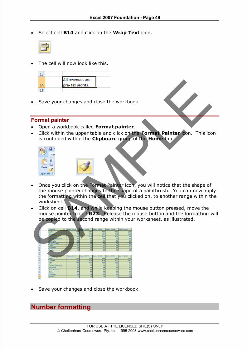
• Select cell B14 and click on the Wrap Text icon.
• The cell will now look like this.
• Save your changes and close the workbook.
Format painter• Open a workbook called Format painter.
• Click within the upper table and click on the Format Painter icon. This iconis contained within the Clipboard group of the Home tab.
• Once you click on the Format Painter icon, you will notice that the shape ofthe mouse pointer changes to the shape of a paintbrush. You can now apply
the formatting within the cell that you clicked on, to another range within theworksheet.
• Click on cell B14, and while keeping the mouse button pressed, move the
mouse pointer to cell G23. Release the mouse button and the formatting willbe copied to the second range within your worksheet, as illustrated.
• Save your changes and close the workbook.
Number formatting

8/11/2019 Excel 2007 Foundation
http://slidepdf.com/reader/full/excel-2007-foundation 52/115
Excel 2007 Foundation - Page 50
FOR USE AT THE LICENSED SITE(S) ONLY
Cheltenham Courseware Pty. Ltd. 1995-2008 www.cheltenhamcourseware.com
Number formatting
• Open a workbook called Number formatting. Click on cell C2. Click on the
down arrow next to the Number Format control. You will see a drop down
menu from which you can select the format. In this case select Number.
• This tells Excel that the data contained within this cell should always now betreated as a number, rather than say text or a date.
Decimal point display
• Click on cell C4. Click on the Decrease Decimal icon so that no decimalplaces are displayed.
• The cell contents should now look like this.
• Set the contents of cell C5 to display 1 decimal point.
• Set the contents of cell C6 to display 2 decimal points.
TIP: To increase the number of decimal points displayed, click on theIncrease Decimal icon.

8/11/2019 Excel 2007 Foundation
http://slidepdf.com/reader/full/excel-2007-foundation 53/115
Excel 2007 Foundation - Page 51
FOR USE AT THE LICENSED SITE(S) ONLY
Cheltenham Courseware Pty. Ltd. 1995-2008 www.cheltenhamcourseware.com
Comma formatting
• Click on cell C8. Click on the Comma Style icon to format the number usingcommas.
• Your number should now look like this.
Currency symbol
• Select cell C10 and format it to display the British Pound symbol. To dothis click on the down arrow next to the Currency icon and select the £
option.
• Select cell C11 and format it to display the Dollar symbol.
• Select cell C12 and format it to display the Euro symbol. Your data will nowlook like this.
Date styles
• Click on cell B17 and type in the text 'The date today is'. Click on cell C17 and type in today's date. When you press the Enter key you may find that
the style of the date changes automatically.
• Right click over cell C17 and from the popup menu displayed select the
Format Cells command.

8/11/2019 Excel 2007 Foundation
http://slidepdf.com/reader/full/excel-2007-foundation 54/115
Excel 2007 Foundation - Page 52
FOR USE AT THE LICENSED SITE(S) ONLY
Cheltenham Courseware Pty. Ltd. 1995-2008 www.cheltenhamcourseware.com
• This will display the Format Cells dialog box.
• Within the Category section of the dialog box, select the Date category.
Select the required format from the Type section of the dialog box.

8/11/2019 Excel 2007 Foundation
http://slidepdf.com/reader/full/excel-2007-foundation 55/115
Excel 2007 Foundation - Page 53
FOR USE AT THE LICENSED SITE(S) ONLY
Cheltenham Courseware Pty. Ltd. 1995-2008 www.cheltenhamcourseware.com
• Click on the OK button to apply the date format. Experiment with applyingdifferent types of date format to the cell.
Percentages
• Click on the cell C15. To change this number from 17 to 17%, type in 17% and press the Enter key. You will then see the contents displayed asillustrated below.
• Save your changes and close the workbook.
Freezing row and column titles
Freezing row and column titles
• Open a workbook called Freezing.
• Scroll down through the data and you will see that the title row, whichcontains a description of each columns contents, scroll out of sight. This

8/11/2019 Excel 2007 Foundation
http://slidepdf.com/reader/full/excel-2007-foundation 56/115
Excel 2007 Foundation - Page 54
FOR USE AT THE LICENSED SITE(S) ONLY
Cheltenham Courseware Pty. Ltd. 1995-2008 www.cheltenhamcourseware.com
makes it difficult to remember what the data in each column represents, if
you cannot see the column title row.
• Make sure that you can see the title row displayed, as illustrated.
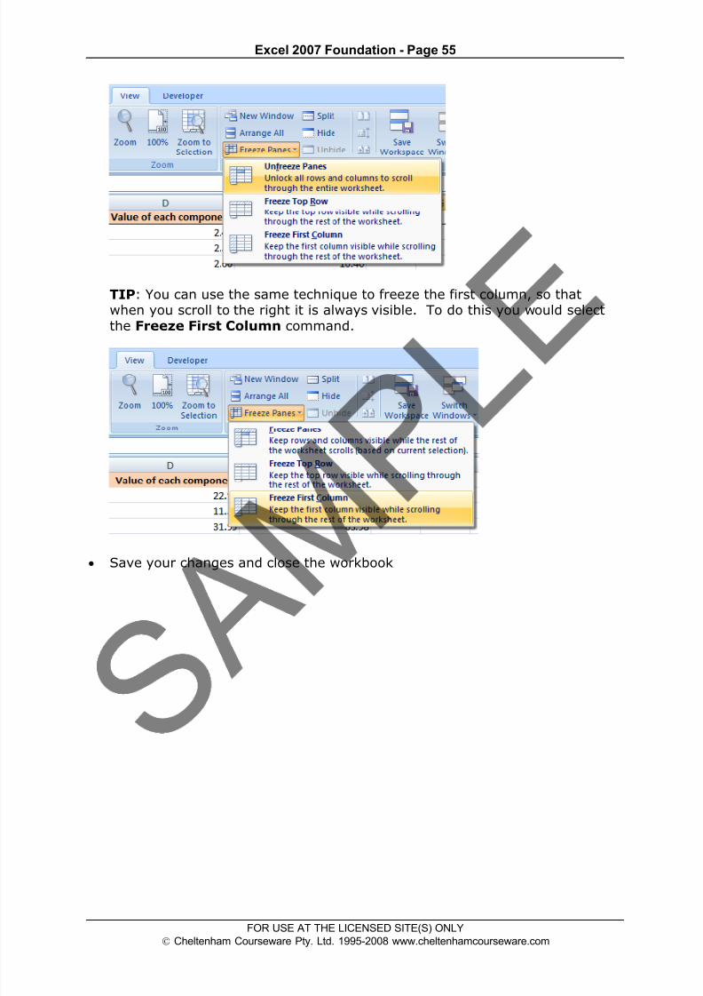
• To freeze the top row so that it remains in sight at all time, click on the View tab and from within the Window group on the Ribbon, click on the FreezePanes command.
• From the drop down list displayed, click on the Freeze Top Row command.
• Scroll down through the data. As you can see the top row stays visible at alltimes now.
• To unfreeze the top row, click on the View tab and from within the Window group on the Ribbon, click on the Unfreeze Panes command.
8/11/2019 Excel 2007 Foundation
http://slidepdf.com/reader/full/excel-2007-foundation 57/115
Excel 2007 Foundation - Page 55
FOR USE AT THE LICENSED SITE(S) ONLY
Cheltenham Courseware Pty. Ltd. 1995-2008 www.cheltenhamcourseware.com
TIP: You can use the same technique to freeze the first column, so thatwhen you scroll to the right it is always visible. To do this you would select
the Freeze First Column command.
• Save your changes and close the workbook

8/11/2019 Excel 2007 Foundation
http://slidepdf.com/reader/full/excel-2007-foundation 58/115
Excel 2007 Foundation - Page 56
FOR USE AT THE LICENSED SITE(S) ONLY
Cheltenham Courseware Pty. Ltd. 1995-2008 www.cheltenhamcourseware.com
Formulas and Functions
Formulas
Creating formulas
• Open a workbook called Formulas. Click on cell E3.
In cell E3 we need to create a formula that will calculate the value of thestock for that particular component. To do this we need to multiply thecontents of cell C3 by the content of cell D3.
• All formulas within Excel start with the 'equals' symbol.
Type in the following formula.
=C3*D3
TIP: the * symbol means 'times'.
Press the Enter key and you will see the result of the calculation in cell E3.
• Click on cell E3 and you will see the formula displayed in the bar above theworksheet.
Easy way to create formulas
• Click on cell E4 and type in the equals sign.
• Click on cell C4 and you see this.

8/11/2019 Excel 2007 Foundation
http://slidepdf.com/reader/full/excel-2007-foundation 59/115
Excel 2007 Foundation - Page 57
FOR USE AT THE LICENSED SITE(S) ONLY
Cheltenham Courseware Pty. Ltd. 1995-2008 www.cheltenhamcourseware.com
• Type in the * symbol, you see this.
• Click on cell D4 and you will see this.
• Press the Enter key and you see the result of the calculation. This method
may seem more complicated at first but when you are creating complexformulas, you will find this method is actually easier and helps to reduce
errors, such as typing incorrect cell references.
Copying formulas
• Click on cell E4.
• Move the mouse pointer to the bottom-right border of this cell and you will
notice that the mouse pointer changes to the shape of a small, solid blackcross. When you see this shape change press the mouse button and while

8/11/2019 Excel 2007 Foundation
http://slidepdf.com/reader/full/excel-2007-foundation 60/115
Excel 2007 Foundation - Page 58
FOR USE AT THE LICENSED SITE(S) ONLY
Cheltenham Courseware Pty. Ltd. 1995-2008 www.cheltenhamcourseware.com
keeping the mouse button depressed, drag down to cell E9. Release themouse button and you will see the formula copied down this range. If youlook at the formula in each cell of the range the cell references areautomatically adjusted to match each row, i.e. row 8 contains the formula
=C8*D8, while row 9 contains the formula =C9*D9.
Your screen will now look like this.
• Close the workbook.
Operators
• Operators sound complicated. In reality they are items such as:
+ (plus)
- (minus)/ (divide)
* (multiply)
You use operators as part of your formulas. There are other operators but
these are the commonly used ones.
Formula error messages
• When writing formulas it is easy to make a mistake: listed below are somecommon error messages.
The contents of the cell cannot be displayed correctly as the column is toonarrow.
Indicates that a cell reference is invalid. This is often displayed when youdelete cells which are involved in a formula.
Excel does not recognise text contained within a formula.

8/11/2019 Excel 2007 Foundation
http://slidepdf.com/reader/full/excel-2007-foundation 61/115
Excel 2007 Foundation - Page 59
FOR USE AT THE LICENSED SITE(S) ONLY
Cheltenham Courseware Pty. Ltd. 1995-2008 www.cheltenhamcourseware.com
Relative, mixed and absolute cell referencing
Relative cell referencing within formulas
•
Open a workbook called Cell referencing.• The first worksheet within the workbook lets us look at relative addressing.
• Click on cell E4. We need to insert the formula for multiplying items incolumn C by the items in columns D. Type in the following formula:
=C4*D4
• Press the Enter key and you will see the result of the calculation in cell E4.
• Click on cell E4, and move the mouse pointer to the bottom-right corner ofcell E4, and when the pointer changes to the shape of a small black cross,press the mouse button, and keep it pressed down. Drag down the page to
cell E12 and then release the mouse button.
• If you click on cell E5 you will see the following =C5*D5.
• If you click on cell E6 you will see the following =C6*D6.
• If you click on cell E7 you will see the following =C7*D7.
• If you click on cell E8 you will see the following =C8*D8.
• If you click on cell E9 you will see the following =C9*D9.
• If you click on cell E10 you will see the following =C10*D10
• If you click on cell E11 you will see the following =C11*D11.
• If you click on cell E12 you will see the following =C12*D12.
• As you can see the referencing is completely relative. This will become
clearer when you have worked through the rest of this section.
Absolute cell referencing within formulas
• Click on the Absolute tab at the bottom of the worksheet.
• Click on cell D4. We need to enter a formula that will take the price and thenadd 5% to the price to give a total value.
The 5% figure has been entered into cell C15.
• Type in the following formula into cell D4.
=C4*C15
If you do the sums, you will find that this formula displays the correctdelivery charge price in cell D4.
• Click on cell D4, and move the mouse pointer to the bottom-right corner ofcell D4, and when the pointer changes to the shape of a small black cross,
press the mouse button, and keep it pressed down. Drag down the page tocell D12 and then release the mouse button. The data will look something

8/11/2019 Excel 2007 Foundation
http://slidepdf.com/reader/full/excel-2007-foundation 62/115
Excel 2007 Foundation - Page 60
FOR USE AT THE LICENSED SITE(S) ONLY
Cheltenham Courseware Pty. Ltd. 1995-2008 www.cheltenhamcourseware.com
like this.
As you can see something has gone very wrong, as the 5% delivery chargeappears to be 0 for most of the items.
• Click on cell D5 and you can see what the problem is. The formula contained
within this cell is:
=C5*C16
Part of the cell reference points to cell C16 (which if you check is empty).
The problem is that because of the relative nature of the formula, thecomponent that should always refer to the contents of the cell in C15 (i.e.the delivery charge percentage), in fact move down as you drag down the
screen to extend your calculations.
• Select the range D4:D12 and press the Del key to delete the cell contents.
• Click on cell D4 and we will try again. This time type in the followingformula.
=C4*$C$15
The dollar signs make the reference to cell C15 absolute.
• Try extending the formula to fill the range down to D12. This time you
should find that the delivery charges are calculated correctly.

8/11/2019 Excel 2007 Foundation
http://slidepdf.com/reader/full/excel-2007-foundation 63/115
Excel 2007 Foundation - Page 61
FOR USE AT THE LICENSED SITE(S) ONLY
Cheltenham Courseware Pty. Ltd. 1995-2008 www.cheltenhamcourseware.com
TIP: You have seen relative and absolute referencing. You can also havemixed references, which contain an absolute and a relative reference.
• Save your changes and close the workbook.
Functions
What is a function?
• A function allows you to calculate a result such as adding numbers together,or finding the average of a range of numbers.
Common functions
• Some commonly used functions include:
AVERAGE: Used to determine the average value of the selected cells
contents.
COLUMNS: Used to return the number of columns within a reference.
COUNT: Used to count how many numbers are in the list.
MAX: Used to return the maximum number from a list.
MIN: Used to return the minimum number from a list.
ROUND: Used to round off numbers to a specified number of decimal points.
SUM: Used to add the contents of selected cells.
To display the available functions, press Ctrl+N to display a blank workbookand then click on the Formulas tab and within the Function Library group
click on the Insert Function icon.
This will display the Insert Function dialog box.
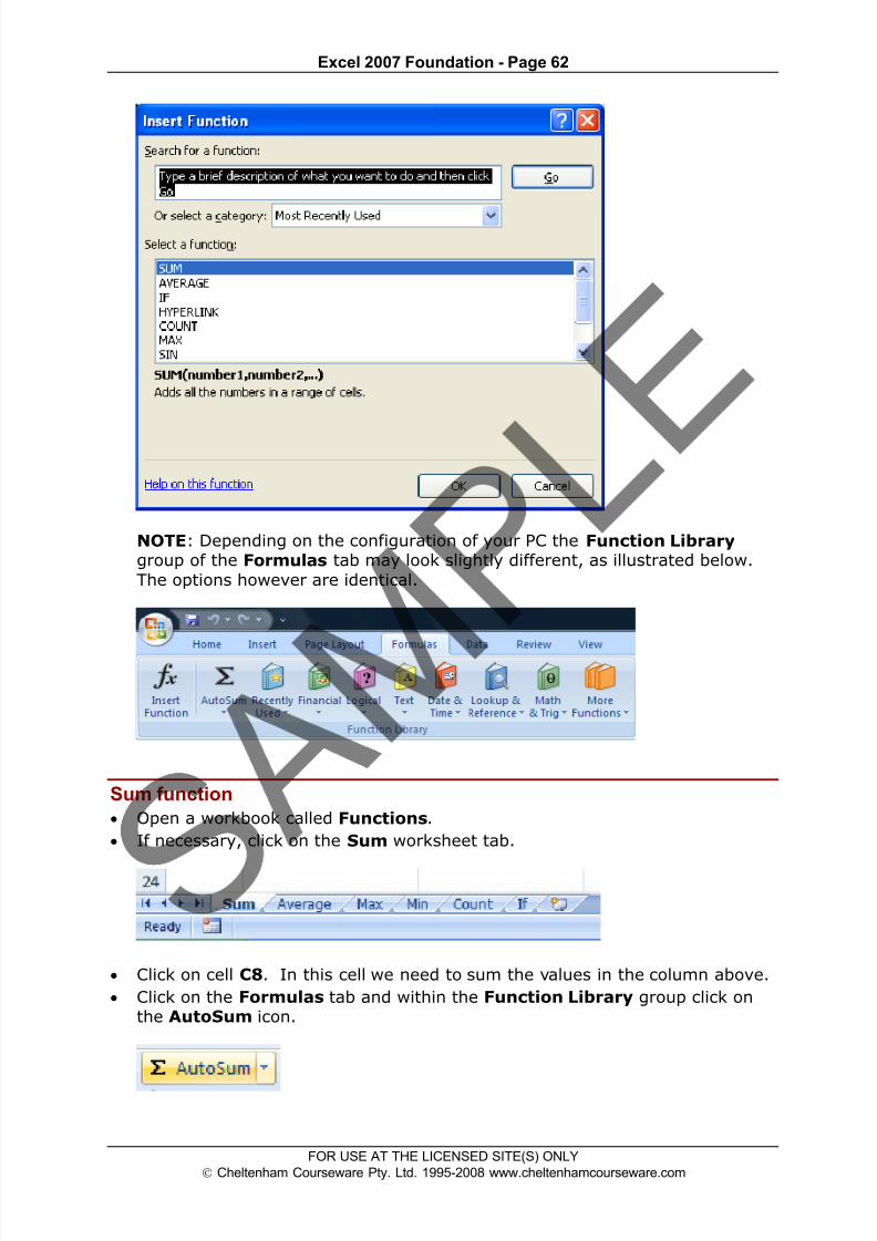
8/11/2019 Excel 2007 Foundation
http://slidepdf.com/reader/full/excel-2007-foundation 64/115
Excel 2007 Foundation - Page 62
FOR USE AT THE LICENSED SITE(S) ONLY
Cheltenham Courseware Pty. Ltd. 1995-2008 www.cheltenhamcourseware.com
NOTE: Depending on the configuration of your PC the Function Library group of the Formulas tab may look slightly different, as illustrated below.
The options however are identical.
Sum function
• Open a workbook called Functions.
• If necessary, click on the Sum worksheet tab.
• Click on cell C8. In this cell we need to sum the values in the column above.
• Click on the Formulas tab and within the Function Library group click onthe AutoSum icon.

8/11/2019 Excel 2007 Foundation
http://slidepdf.com/reader/full/excel-2007-foundation 65/115
Excel 2007 Foundation - Page 63
FOR USE AT THE LICENSED SITE(S) ONLY
Cheltenham Courseware Pty. Ltd. 1995-2008 www.cheltenhamcourseware.com
TIP: Click on the AutoSum icon, not the down arrow beside the icon.
• You will see the following displayed on your screen.
• Press the Enter key and you will see the AutoSum result in cell C8.
• Click on cell C8, and you will see the function displayed in the bar just aboveyour worksheet.
As you can see the function is:

8/11/2019 Excel 2007 Foundation
http://slidepdf.com/reader/full/excel-2007-foundation 66/115
Excel 2007 Foundation - Page 64
FOR USE AT THE LICENSED SITE(S) ONLY
Cheltenham Courseware Pty. Ltd. 1995-2008 www.cheltenhamcourseware.com
=SUM(C4:C7)
• This function tells Excel to sum the values in the range C4:C7.
Average function• Click on the Average worksheet tab.
• Click on cell C8. In this cell we want to display the average number of sales
within the regions.
• Click on the Formulas tab and within the Function Library group click on
the arrow next to the AutoSum icon. You will see a drop down listdisplayed. Click on the Average command.
• You will see the following displayed on your screen.

8/11/2019 Excel 2007 Foundation
http://slidepdf.com/reader/full/excel-2007-foundation 67/115
Excel 2007 Foundation - Page 65
FOR USE AT THE LICENSED SITE(S) ONLY
Cheltenham Courseware Pty. Ltd. 1995-2008 www.cheltenhamcourseware.com
• Press the Enter key and you will see the average value displayed in cell C8.
• Click on cell C8, and you will see the function displayed in the bar just aboveyour worksheet.
As you can see the function is:
=AVERAGE(C4:C7)
• This function tells Excel to sum the average in the range C4:C7.

8/11/2019 Excel 2007 Foundation
http://slidepdf.com/reader/full/excel-2007-foundation 68/115
Excel 2007 Foundation - Page 66
FOR USE AT THE LICENSED SITE(S) ONLY
Cheltenham Courseware Pty. Ltd. 1995-2008 www.cheltenhamcourseware.com
Max function
• Click on the Max worksheet tab.
• Click on cell C8. In this cell we want to display the highest number of sales
within a region.
• Click on the Formulas tab and within the Function Library group click onthe down arrow next to (or under) the AutoSum icon. You will see a drop
down list displayed. Click on the Max command.
• You will see the following displayed on your screen.
• Press the Enter key and you will see the maximum value displayed in cellC8.

8/11/2019 Excel 2007 Foundation
http://slidepdf.com/reader/full/excel-2007-foundation 69/115
Excel 2007 Foundation - Page 67
FOR USE AT THE LICENSED SITE(S) ONLY
Cheltenham Courseware Pty. Ltd. 1995-2008 www.cheltenhamcourseware.com
• Click on cell C8, and you will see the function displayed in the bar just aboveyour worksheet.
As you can see the function is:
=MAX(C4:C7)
• This function tells Excel to display the maximum value within the range
C4:C7.
Min function
• The MIN function will display the minimum number within a range.
• Click on the Min worksheet tab.
• Click on cell C8. In this cell we want to display the lowest number of sales
within a region.
• Click on the Formulas tab and within the Function Library group click on
the down arrow next to (or under) the AutoSum icon. You will see a dropdown list displayed. Click on the Min command.

8/11/2019 Excel 2007 Foundation
http://slidepdf.com/reader/full/excel-2007-foundation 70/115
Excel 2007 Foundation - Page 68
FOR USE AT THE LICENSED SITE(S) ONLY
Cheltenham Courseware Pty. Ltd. 1995-2008 www.cheltenhamcourseware.com
• You will see the following displayed on your screen.
• Press the Enter key and you will see the minimum value displayed in cell C8.
• Click on cell C8, and you will see the function displayed in the bar just aboveyour worksheet.
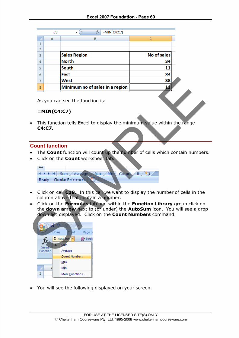
8/11/2019 Excel 2007 Foundation
http://slidepdf.com/reader/full/excel-2007-foundation 71/115
Excel 2007 Foundation - Page 69
FOR USE AT THE LICENSED SITE(S) ONLY
Cheltenham Courseware Pty. Ltd. 1995-2008 www.cheltenhamcourseware.com
As you can see the function is:
=MIN(C4:C7)
• This function tells Excel to display the minimum value within the range
C4:C7.
Count function
• The Count function will count up the number of cells which contain numbers.
• Click on the Count worksheet tab.
• Click on cell C19. In this cell we want to display the number of cells in thecolumn above that contain a number.
• Click on the Formulas tab and within the Function Library group click onthe down arrow next to (or under) the AutoSum icon. You will see a drop
down list displayed. Click on the Count Numbers command.
• You will see the following displayed on your screen.

8/11/2019 Excel 2007 Foundation
http://slidepdf.com/reader/full/excel-2007-foundation 72/115
Excel 2007 Foundation - Page 70
FOR USE AT THE LICENSED SITE(S) ONLY
Cheltenham Courseware Pty. Ltd. 1995-2008 www.cheltenhamcourseware.com
• WARNING: In all the previous examples, there was a column containingvalues immediately above the cell into which we inserted the function. Inthis case some of the cells within the column are empty and Excel, as you
can see has only applied the Count function to the range C17:C18. Thereason for this is that the next cell up, i.e. cell C16 is empty.
We need to tell Excel that the range we are interested in, actually extents
from C5:C18.
To do this, click on cell C18 and while holding down the mouse button dragup to cell C5. Then release the mouse button. Your screen should now look
like this.

8/11/2019 Excel 2007 Foundation
http://slidepdf.com/reader/full/excel-2007-foundation 73/115
Excel 2007 Foundation - Page 71
FOR USE AT THE LICENSED SITE(S) ONLY
Cheltenham Courseware Pty. Ltd. 1995-2008 www.cheltenhamcourseware.com
• Press the Enter key and you will see the count value displayed in cell C19.
• Click on cell C19, and you will see the function displayed in the bar justabove your worksheet.
As you can see the function is:
=COUNT(C5:C18)
• This function tells Excel to display the number of cells containing a valuewithin the range C5:C18.
NOTE: If you made a mistake, click on cell C18 and press the Del key. Then

8/11/2019 Excel 2007 Foundation
http://slidepdf.com/reader/full/excel-2007-foundation 74/115
Excel 2007 Foundation - Page 72
FOR USE AT THE LICENSED SITE(S) ONLY
Cheltenham Courseware Pty. Ltd. 1995-2008 www.cheltenhamcourseware.com
try again.
• Use the same technique to count up the number of people who could not
attend, and display the value in cell D19.
What are 'IF functions'?
• Excel has a number of functions which allow us to evaluate values and makedecisions based on the result of the evaluation. The IF( ) FUNCTION is oneof these.
IF( ) SYNTAXThe format (Syntax) of the IF( ) function is as follows:
IF(LOGICAL_TEST, ACTION_IF_TRUE, ACTION_IF_FALSE)
LOGICAL_TESTThe logical_test evaluates an expression to see if it passes the test, i.e. isTRUE or does not pass the test, i.e. is FALSE
• ACTION_IF_TRUEAction_if_true can be a value or an operation. Whichever, the result is placedin the cell which contains the IF( ) Function if the logical_test is true.
ACTION_IF_FALSEAction_if_false can be a value or an operation. Whichever, the result is placed
in the cell which contains the IF( ) Function if the logical_test is false.
Using the IF function
• Click on the If worksheet tab.
• In cells J8:J13 we need to display the word PASS or FAIL, depending onwhether the average is over 70%.

8/11/2019 Excel 2007 Foundation
http://slidepdf.com/reader/full/excel-2007-foundation 75/115
Excel 2007 Foundation - Page 73
FOR USE AT THE LICENSED SITE(S) ONLY
Cheltenham Courseware Pty. Ltd. 1995-2008 www.cheltenhamcourseware.com
• Click on the cell J8.• Click on the Logical icon within the Function Library group of the
Formulas tab.
TIP: Remember that depending on the configuration of your PC, theFunction Library may look like this.
• This will display a drop down list. Select the IF command.

8/11/2019 Excel 2007 Foundation
http://slidepdf.com/reader/full/excel-2007-foundation 76/115
Excel 2007 Foundation - Page 74
FOR USE AT THE LICENSED SITE(S) ONLY
Cheltenham Courseware Pty. Ltd. 1995-2008 www.cheltenhamcourseware.com
• This will display the Function Arguments dialog box.
• In the LOGICAL_TEST section of the dialog box, we enter the logical test,
i.e. I8>70
In the VALUE_IF_TRUE section of the dialog box, we enter the word PASS.
In the VALUE_IF_FALSE section of the dialog box, we enter the word FAIL.

8/11/2019 Excel 2007 Foundation
http://slidepdf.com/reader/full/excel-2007-foundation 77/115
Excel 2007 Foundation - Page 75
FOR USE AT THE LICENSED SITE(S) ONLY
Cheltenham Courseware Pty. Ltd. 1995-2008 www.cheltenhamcourseware.com
• Your dialog box will now look like this.
• Click on the OK button to continue. Your screen will now look like this.
• Use the normal Excel drag techniques to extend this function to the cells
I9:J13. Your screen will now look like this.
• Save your changes and close the workbook.

8/11/2019 Excel 2007 Foundation
http://slidepdf.com/reader/full/excel-2007-foundation 78/115
Excel 2007 Foundation - Page 76
FOR USE AT THE LICENSED SITE(S) ONLY
Cheltenham Courseware Pty. Ltd. 1995-2008 www.cheltenhamcourseware.com
Charts
Using Charts
Inserting a column chart
• Open a workbook called Chart.
• If necessary, click on the Column Chart worksheet tab (at the bottom-leftof your screen).
• Click within the table of data.
• Click on the Insert tab and you will see the Charts group displayed within
the Ribbon.
• Click on the Column icon and you will see a drop down displaying a range ofcolumn chart options.
•
Click on the first option, the
2-D Clustered format, as illustrated.

8/11/2019 Excel 2007 Foundation
http://slidepdf.com/reader/full/excel-2007-foundation 79/115
Excel 2007 Foundation - Page 77
FOR USE AT THE LICENSED SITE(S) ONLY
Cheltenham Courseware Pty. Ltd. 1995-2008 www.cheltenhamcourseware.com
• You will see the following chart inserted into your worksheet.
• Click on the Undo icon (top-left of your screen), and experiment withinserting other types of column chart such as a 3-D chart, as illustratedbelow.
Inserting a line chart
• Click on the Line Chart worksheet tab at the bottom of your screen.

8/11/2019 Excel 2007 Foundation
http://slidepdf.com/reader/full/excel-2007-foundation 80/115
Excel 2007 Foundation - Page 78
FOR USE AT THE LICENSED SITE(S) ONLY
Cheltenham Courseware Pty. Ltd. 1995-2008 www.cheltenhamcourseware.com
• Experiment with inserting different types of line chart. An example is
illustrated below.
Inserting a bar chart
• Click on the Bar Chart worksheet tab at the bottom of your screen.
• Experiment with inserting different types of bar chart. An example is
illustrated below.

8/11/2019 Excel 2007 Foundation
http://slidepdf.com/reader/full/excel-2007-foundation 81/115
Excel 2007 Foundation - Page 79
FOR USE AT THE LICENSED SITE(S) ONLY
Cheltenham Courseware Pty. Ltd. 1995-2008 www.cheltenhamcourseware.com
Inserting a pie chart
• Click on the Pie Chart worksheet tab at the bottom of your screen.
• Experiment with inserting different types of pie chart. An example isillustrated below.
• Save your changes and close the workbook.
Resizing a chart
• Open a workbook called Chart Manipulation.
• To resize a chart click on it to select it.
• Move the mouse pointer to one of the four corners of the chart. You will
notice that the mouse pointer changes to the shape of a diagonal line with anarrow at each end. When you see the mouse pointer change, press themouse button and while keeping the button pressed move diagonally acrossthe screen. Move away from the centre of the chart to make the chart larger
and toward the centre of the chart to make the chart smaller. When yourelease the mouse button the chart will be resized.
Deleting a chart
• Select the chart and press the Del key.
• Save your changes and close the workbook.
Chart title or labels
• Open a workbook called Modifying charts.

8/11/2019 Excel 2007 Foundation
http://slidepdf.com/reader/full/excel-2007-foundation 82/115
Excel 2007 Foundation - Page 80
FOR USE AT THE LICENSED SITE(S) ONLY
Cheltenham Courseware Pty. Ltd. 1995-2008 www.cheltenhamcourseware.com
• If necessary, click on the Modifying a Chart worksheet tab (at the bottom-left of your screen).
• You can see a column chart displayed within the workbook. Select the charttitle, as illustrated.
• Press the Del key to remove the chart title. Your chart will now look like this.
• To insert a chart title, click on chart and then click on the Layout tab. Clickon the Chart Title icon within the Layout Ribbon.
• Select the required option from the drop down list displayed, such as AboveChart.

8/11/2019 Excel 2007 Foundation
http://slidepdf.com/reader/full/excel-2007-foundation 83/115
Excel 2007 Foundation - Page 81
FOR USE AT THE LICENSED SITE(S) ONLY
Cheltenham Courseware Pty. Ltd. 1995-2008 www.cheltenhamcourseware.com
• Your chart title is once again displayed, as illustrated.
TIP: To modify the chart title text, click within the Chart Title and simplyedit the text in the normal way. You can also apply text formatting to theChart Title as required. An example is shown below.

8/11/2019 Excel 2007 Foundation
http://slidepdf.com/reader/full/excel-2007-foundation 84/115
Excel 2007 Foundation - Page 82
FOR USE AT THE LICENSED SITE(S) ONLY
Cheltenham Courseware Pty. Ltd. 1995-2008 www.cheltenhamcourseware.com
Chart background colour
• Click on the chart to select it. Right click over an empty part of the chartbackground, and you will see a popup menu displayed.
• Click on the Format Chart Area command.
TIP: If you do not see this command, right click on a different, empty part ofthe chart, until you do see this command.
•
You will see the Format Chart Area dialog box displayed.
• If necessary, click on the Solid fill button and you will see extra controlsdisplayed within the dialog box.

8/11/2019 Excel 2007 Foundation
http://slidepdf.com/reader/full/excel-2007-foundation 85/115
Excel 2007 Foundation - Page 83
FOR USE AT THE LICENSED SITE(S) ONLY
Cheltenham Courseware Pty. Ltd. 1995-2008 www.cheltenhamcourseware.com
• Click on the down arrow next to the Color control and select a light colour
from the options displayed.
• Click on the Close button to apply the colour, as illustrated below.

8/11/2019 Excel 2007 Foundation
http://slidepdf.com/reader/full/excel-2007-foundation 86/115
Excel 2007 Foundation - Page 84
FOR USE AT THE LICENSED SITE(S) ONLY
Cheltenham Courseware Pty. Ltd. 1995-2008 www.cheltenhamcourseware.com
Changing the column, bar, line or pie slice colours in a chart
• Click on the second worksheet tab, called Column Chart.
• Click on one of the columns within the chart. You should see all the columnsare selected, as illustrated.
• Right click over one of the selected columns and from the popup menu
displayed select the Format Data Series command.
• This will display the Format Data Series dialog box.

8/11/2019 Excel 2007 Foundation
http://slidepdf.com/reader/full/excel-2007-foundation 87/115
Excel 2007 Foundation - Page 85
FOR USE AT THE LICENSED SITE(S) ONLY
Cheltenham Courseware Pty. Ltd. 1995-2008 www.cheltenhamcourseware.com
• Click on the Fill command within the dialog box, as illustrated.
• Click on the Solid fill command and extra controls will be displayed, asillustrated.
• Click on the down arrow in the Color section and select a colour for your
columns.

8/11/2019 Excel 2007 Foundation
http://slidepdf.com/reader/full/excel-2007-foundation 88/115
Excel 2007 Foundation - Page 86
FOR USE AT THE LICENSED SITE(S) ONLY
Cheltenham Courseware Pty. Ltd. 1995-2008 www.cheltenhamcourseware.com
• When you click on the Close icon the selected colour will be applied, asillustrated.
• Click on the Line Chart worksheet tab and change the colour of the line.
• Click on the Bar Chart worksheet tab and change the colour of the bars.
• Click on the Pie Chart worksheet tab to display the pie chart. The wholepoint of a pie chart is that each segment of the pie chart should be a differentcolour. Bearing this is mind click once on the pie chart to select all thesegments within the pie chart. Then click again on a particular segment to
select just that segment. At this point you can then right click and changethe colour of just that segment. An example is illustrated below.

8/11/2019 Excel 2007 Foundation
http://slidepdf.com/reader/full/excel-2007-foundation 89/115
Excel 2007 Foundation - Page 87
FOR USE AT THE LICENSED SITE(S) ONLY
Cheltenham Courseware Pty. Ltd. 1995-2008 www.cheltenhamcourseware.com
• Save your changes and close the workbook.
Changing the chart type• Open a workbook called Changing charts. This workbook contains a column
chart. Click on the chart to select it. Click on the Design tab. Click on the
Change Chart Type icon displayed within the Type group of the Design Ribbon.
• This will display the Change Chart Type dialog box.
• Select a different type of chart, such as a Bar chart and then click on the OK button.

8/11/2019 Excel 2007 Foundation
http://slidepdf.com/reader/full/excel-2007-foundation 90/115
Excel 2007 Foundation - Page 88
FOR USE AT THE LICENSED SITE(S) ONLY
Cheltenham Courseware Pty. Ltd. 1995-2008 www.cheltenhamcourseware.com
• Experiment with applying different types of chart.• Save your changes and close the workbook.
Modifying Charts using the Layout tab
• Open a workbook called Formatting Charts.
• Select the chart and then click on the Layout tab.
• The Layout tab includes many options for controlling how the various chart
elements are displayed.
• Click on the Chart Title button in the Labels group of the Ribbon. A menuwill be display allowing you to control where or if the chart title is displayed.The default is Above Chart, try selecting the other options and observe the
effect on the chart.

8/11/2019 Excel 2007 Foundation
http://slidepdf.com/reader/full/excel-2007-foundation 91/115
Excel 2007 Foundation - Page 89
FOR USE AT THE LICENSED SITE(S) ONLY
Cheltenham Courseware Pty. Ltd. 1995-2008 www.cheltenhamcourseware.com
• Click on the Axis Titles button in the Labels group of the Ribbon. A menuwill be display allowing you to control how the labels for each axis aredisplayed. Experiment with some of the available options and view theireffect on the chart.
• Click on the Legend button in the Labels group of the Ribbon. A menu willbe display allowing you to control where the chart legend is displayed.
Experiment with some of the available options and view their effect on thechart.
• Click on the Data Labels button in the Labels group of the Ribbon. A menuwill be displayed allowing you to choose if labels should be applied to data in
the chart.
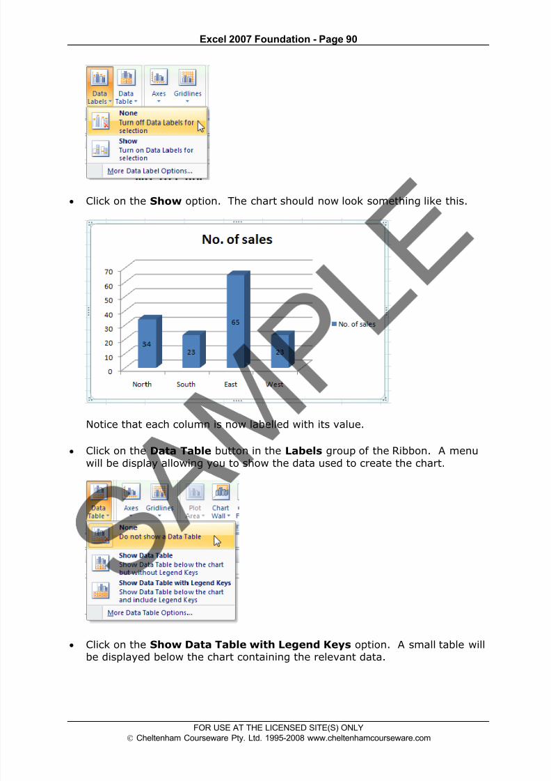
8/11/2019 Excel 2007 Foundation
http://slidepdf.com/reader/full/excel-2007-foundation 92/115
Excel 2007 Foundation - Page 90
FOR USE AT THE LICENSED SITE(S) ONLY
Cheltenham Courseware Pty. Ltd. 1995-2008 www.cheltenhamcourseware.com
• Click on the Show option. The chart should now look something like this.
Notice that each column is now labelled with its value.
• Click on the Data Table button in the Labels group of the Ribbon. A menu
will be display allowing you to show the data used to create the chart.
• Click on the Show Data Table with Legend Keys option. A small table willbe displayed below the chart containing the relevant data.

8/11/2019 Excel 2007 Foundation
http://slidepdf.com/reader/full/excel-2007-foundation 93/115
Excel 2007 Foundation - Page 91
FOR USE AT THE LICENSED SITE(S) ONLY
Cheltenham Courseware Pty. Ltd. 1995-2008 www.cheltenhamcourseware.com
• Click on the Gridlines button in the Axes group of the Ribbon. A menu willbe display allowing you to control how the gridlines for each axis are
displayed. Experiment with some of the available options and view theireffect on the chart.
• Close the workbook and save any changes you may have made.
Copying and moving charts within a worksheet
• Open a workbook called Copying and moving charts 1.
• Click on the chart to select it.
• To move the chart within the worksheet, click on the chart and drag the chartto a new position in the worksheet.
• To copy the chart within the worksheet, click on the chart to select it andpress Ctrl+C to copy the chart to the Clipboard. Deselect the chart and then
press Ctrl+V to paste the chart from the Clipboard. You should now see two

8/11/2019 Excel 2007 Foundation
http://slidepdf.com/reader/full/excel-2007-foundation 94/115
Excel 2007 Foundation - Page 92
FOR USE AT THE LICENSED SITE(S) ONLY
Cheltenham Courseware Pty. Ltd. 1995-2008 www.cheltenhamcourseware.com
copies of the chart. You can move them so that they are not layered on top
of each other.
Copying and moving charts between worksheets
• Click on the chart to select it.
• To copy the chart to another worksheet within the workbook, click on
the chart to select it and press Ctrl+C to copy the chart to the Clipboard.
• Click on the Sheet2 tab at the bottom of the worksheet.
• Press Ctrl+V to paste the chart from the Clipboard. You can move the chartif required within this worksheet.
• To move the chart to another worksheet within the workbook, click on
the Sheet1 tab at the bottom of the worksheet. Click on the chart to select itand press Ctrl+X to cut (i.e. move) the chart to the Clipboard.
• Click on the Sheet3 tab at the bottom of the worksheet.
• Press Ctrl+V to paste the chart from the Clipboard. You can move the chartif required within this worksheet.
Copying and moving charts between workbooks
• Select a chart within the workbook. Press Ctrl+C to copy the chart to theClipboard. Open a second workbook called Copying and moving charts 2.
Press Ctrl+V to paste the chart into the second workbook.
NOTE: To move a chart between workbooks, use the same procedure, but
Cut rather than Copy the chart, using the Ctrl+X keyboard shortcut for
cutting a selected item to the Clipboard.
• Close all open workbooks and save any changes you have made.

8/11/2019 Excel 2007 Foundation
http://slidepdf.com/reader/full/excel-2007-foundation 95/115
Excel 2007 Foundation - Page 93
FOR USE AT THE LICENSED SITE(S) ONLY
Cheltenham Courseware Pty. Ltd. 1995-2008 www.cheltenhamcourseware.com
Customizing Excel
Modifying basic options
• You can customize the way Excel looks and performs. To do this click on theMicrosoft Office button and within the dialog box displayed click on the
Excel Options button (bottom-right of the dialog box).
• This will display the Excel Options dialog box.
• You can use this to customise items such as the type of font used, the fontsize used and the number of worksheets displayed within a new workbook.

8/11/2019 Excel 2007 Foundation
http://slidepdf.com/reader/full/excel-2007-foundation 96/115
Excel 2007 Foundation - Page 94
FOR USE AT THE LICENSED SITE(S) ONLY
Cheltenham Courseware Pty. Ltd. 1995-2008 www.cheltenhamcourseware.com
• Try altering the number of worksheets contained within a new workbook to 4rather than 3.
Then close the dialog box and press Ctrl+N to create a new workbook. Youshould see 4 worksheets, as illustrated.
Close the new workbook without saving any changes you have made.
Reset the default for new workbooks, back to 3 worksheets per workbook.
• Reopen the Excel Options dialog box, and click on the Save option(displayed down the left side of the dialog box).
You can use this page to set the default folder location to be used when
saving your workbooks.

8/11/2019 Excel 2007 Foundation
http://slidepdf.com/reader/full/excel-2007-foundation 97/115
Excel 2007 Foundation - Page 95
FOR USE AT THE LICENSED SITE(S) ONLY
Cheltenham Courseware Pty. Ltd. 1995-2008 www.cheltenhamcourseware.com
• As you can see there are lots more useful options that you can customise tomake your use of Excel easier and more productive. If you have timeinvestigate some of the other customisation options available.
• Before you move on, click on the Resources button (within the left part of
the dialog box). As you can see this has an option that allows you to checkfor updates.
• Close the dialog box before continuing.
Minimising the Ribbon
• Sometimes you want ‘more writing space’. To help achieve this you can right
click over the Ribbon and from the popup menu displayed, click on theMinimize the Ribbon command.
• The Ribbon display will change from this.
To this.

8/11/2019 Excel 2007 Foundation
http://slidepdf.com/reader/full/excel-2007-foundation 98/115
Excel 2007 Foundation - Page 96
FOR USE AT THE LICENSED SITE(S) ONLY
Cheltenham Courseware Pty. Ltd. 1995-2008 www.cheltenhamcourseware.com
• To display the Ribbon again, right click over any of the tab commands and
from the popup menu displayed, re-click on the Minimize the Ribbon command (to remove the tick).
AutoCorrect options
• Microsoft Excel has an AutoCorrect facility that allows common typing errors
to be automatically corrected. For instance if you type in 'teh' instead of'the', Microsoft Excel will automatically correct your spelling error.
• To open the AutoCorrect dialog box, click on the Office Button (top-left ofyour screen). Click on the Excel Options button at the bottom of the dialogbox.
• Click on the Proofing option, and then click on the AutoCorrect Options
button.
This will display the AutoCorrect dialog box.

8/11/2019 Excel 2007 Foundation
http://slidepdf.com/reader/full/excel-2007-foundation 99/115
Excel 2007 Foundation - Page 97
FOR USE AT THE LICENSED SITE(S) ONLY
Cheltenham Courseware Pty. Ltd. 1995-2008 www.cheltenhamcourseware.com
• As you can see this has a number of options such as the ability to correctwords where you have accidentally typed in the first two letters in capitals. Itwill also automatically capitalise the first letter within a sentence and also the
first letter within a table cell and the days of the week. A very useful featureis to automatically correct the effect of accidentally pressing the Caps Lock
key.
• In the lower part of the dialog box is a scrollable section which tells you what
Microsoft Excel will act on and change automatically.
• Add some words that you commonly spell incorrectly, into the Replace section of the dialog box, along with the correct spelling in the With section
of the dialog box.

8/11/2019 Excel 2007 Foundation
http://slidepdf.com/reader/full/excel-2007-foundation 100/115
Excel 2007 Foundation - Page 98
FOR USE AT THE LICENSED SITE(S) ONLY
Cheltenham Courseware Pty. Ltd. 1995-2008 www.cheltenhamcourseware.com
Printing
Worksheet Setup
Worksheet margins
• Open a workbook called Print setup.
• Click on the Page Layout tab, and from within the Page Setup group of theRibbon, click on the Margins icon.
• This will display a drop down from which you can select Normal, Wide or
Narrow.
• Clicking on the Custom Margins command displays the Margins tab withinthe Page Setup dialog box. You can use this dialog box to set custom top,bottom, left and right margins.

8/11/2019 Excel 2007 Foundation
http://slidepdf.com/reader/full/excel-2007-foundation 101/115
Excel 2007 Foundation - Page 99
FOR USE AT THE LICENSED SITE(S) ONLY
Cheltenham Courseware Pty. Ltd. 1995-2008 www.cheltenhamcourseware.com
TIP: You can also use this dialog box to set Header and Footer values, as
well as options to centre the table on the page vertically and / or horizontally.
Experiment with setting margins.
TIP: Be sure not to make the margin size to small or you may have problems
printing the worksheet.
Worksheet orientation
• Click on the Page Layout tab, and from within the Page Setup group of theRibbon, click on the Orientation icon. You can select either Portrait or
Landscape orientation, as illustrated.

8/11/2019 Excel 2007 Foundation
http://slidepdf.com/reader/full/excel-2007-foundation 102/115
Excel 2007 Foundation - Page 100
FOR USE AT THE LICENSED SITE(S) ONLY
Cheltenham Courseware Pty. Ltd. 1995-2008 www.cheltenhamcourseware.com
• Try setting the orientation to Landscape. To see the effect in PrintPreview mode, press the Ctrl+F2 keyboard shortcut. To return to theprevious view, click on the Close Print Preview icon.
• Before continuing reset the orientation back to Portrait.
Worksheet page size
• Click on the Page Layout tab, and from within the Page Setup group of theRibbon, click on the Size icon. You can select the required page size fromthe drop down options displayed, as illustrated.
Headers and Footers
• Click on the Insert tab and from within the Text group of the Ribbon, clickon the Header & Footer icon.

8/11/2019 Excel 2007 Foundation
http://slidepdf.com/reader/full/excel-2007-foundation 103/115
Excel 2007 Foundation - Page 101
FOR USE AT THE LICENSED SITE(S) ONLY
Cheltenham Courseware Pty. Ltd. 1995-2008 www.cheltenhamcourseware.com
• You will see the Header area displayed at the top of the worksheet, asillustrated.
• Type in the text for you header, such as 'Stock Levels for January'.
• If you scroll down the page you will see the message 'Click to add footer'displayed at the bottom of the worksheet.
• Click within the footer area and type in your name. As example is illustratedbelow.
• To modify a header or footer at any time just click over an existing header orfooter and edit as required.
TIP: Remember that to see headers and footers, you may need to click onthe View tab and then click on the Page Layout icon.
To change back to the normal view click on the View tab and then click on
the Normal icon.

8/11/2019 Excel 2007 Foundation
http://slidepdf.com/reader/full/excel-2007-foundation 104/115
Excel 2007 Foundation - Page 102
FOR USE AT THE LICENSED SITE(S) ONLY
Cheltenham Courseware Pty. Ltd. 1995-2008 www.cheltenhamcourseware.com
Header and footer fields
• When you are inserting or editing a footer or header, you will notice that yousee the Header and Footer Tools Ribbon. Within this Ribbon is the Header& Footer Elements group, as illustrated below.
• You can use the icons in this section in insert an Excel field, such as the PageNumber. The great thing about fields is that they automatically updatewhen required. For instance if you insert a Page Number field, then as you
add more pages, the page number displayed on each page will increment.
• Another very useful field is the File Name field. This displays the file nameof the document in your header or footer, when you print, and is very useful
when you have printed out a copy of a worksheet and then several monthslater are trying to remember the file name you used to save the worksheetas.
NOTE: When you insert a field, such as the File Name field, you may see
the field code rather than the actual file name. When you print theworksheet however, this code is replaced by the actual file name.
• The File Path will display the file name and also the path to the folder inwhich the file is stored.
• Experiment with inserting different fields into your header or footer.
Scaling your worksheet to fit a page(s)
• Click on the Microsoft Office Button and then click on the arrow next tothe Print command. From the submenu, select Print Preview.

8/11/2019 Excel 2007 Foundation
http://slidepdf.com/reader/full/excel-2007-foundation 105/115
Excel 2007 Foundation - Page 103
FOR USE AT THE LICENSED SITE(S) ONLY
Cheltenham Courseware Pty. Ltd. 1995-2008 www.cheltenhamcourseware.com
• If you look at the bottom-left of the screen you will notice that in theexample shown, the data requires a total of 4 pages to print.
• To close the Print Preview view, click on the Close Print Preview button
• Excel has a facility that lets you determine how many pages you want thedata to print over. If required you can shrink the size of the data so that itall fits on one page. It may be hard to read due to the small type size, butyou can do this. Click on the Page Layout tab and within the Scale to Fit group to display the following options.
• Click on the down arrow to the right of the Width control, and select 1page.

8/11/2019 Excel 2007 Foundation
http://slidepdf.com/reader/full/excel-2007-foundation 106/115
Excel 2007 Foundation - Page 104
FOR USE AT THE LICENSED SITE(S) ONLY
Cheltenham Courseware Pty. Ltd. 1995-2008 www.cheltenhamcourseware.com
• Click on the down arrow to the right of the Height control, and select 1page.
• Display the worksheet in Print Preview view and you should see that the
worksheet will now print on a single page.
• Close the Print Preview view.
• Save your changes and close the workbook.
Preparing to print a worksheet
Visually check your calculations
• Open a workbook called Printing.
• Click on cell E2. Clearly the formula within this cell is wrong. The formula it
contains is
=C2*F2
It should be:

8/11/2019 Excel 2007 Foundation
http://slidepdf.com/reader/full/excel-2007-foundation 107/115
Excel 2007 Foundation - Page 105
FOR USE AT THE LICENSED SITE(S) ONLY
Cheltenham Courseware Pty. Ltd. 1995-2008 www.cheltenhamcourseware.com
=C2*D2
Fix the formula.
Always visually check over worksheet data and try to look for formulacalculation results that do not make sense.
Gridline display when printing
• To see how the worksheet will look when printed view the worksheet in PrintPreview view. To do this click press Ctrl+F2. As you can see the worksheetwill print without displaying gridlines.
• Click on the Close Print Preview button to exit from the Print Previewmode.
• Click on the Page Layout tab. Within the Sheet Options group, click on the
Print check box under the Gridlines heading, as illustrated.
• View the worksheet in Print Preview view by pressing Ctrl+F2. As you can
see the worksheet will now print displaying gridlines.

8/11/2019 Excel 2007 Foundation
http://slidepdf.com/reader/full/excel-2007-foundation 108/115
Excel 2007 Foundation - Page 106
FOR USE AT THE LICENSED SITE(S) ONLY
Cheltenham Courseware Pty. Ltd. 1995-2008 www.cheltenhamcourseware.com
• Exit the Print Preview view.
• Before continuing, re-click on the Print Gridlines check box so that the
worksheet will print without displaying gridlines.
Printing titles on every page when printing
• View the worksheet in Print Preview view by pressing Ctrl+F2. As you cansee the top row, containing the column titles is displayed on the first page.
• Press the Page Down key to view the second page. As you can see thecolumns are displayed without a top row explaining what each column relatesto.

8/11/2019 Excel 2007 Foundation
http://slidepdf.com/reader/full/excel-2007-foundation 109/115
Excel 2007 Foundation - Page 107
FOR USE AT THE LICENSED SITE(S) ONLY
Cheltenham Courseware Pty. Ltd. 1995-2008 www.cheltenhamcourseware.com
• We need to fix this as it would be very inconvenient to print out a long reportand always have to refer to the first page to know what each column relatesto. Close the Print Preview view.
• Click on the Page Layout tab. Within the Page Setup group, click on the
Print Titles icon, as illustrated.
• This will display the Page Setup dialog box.
• If necessary move dialog box so that you can see the title row within theworksheet.
TIP: To move a dialog box, click on the Title Bar at the top of the dialog boxand while pressing the mouse button, drag with the mouse. When yourelease the mouse button the dialog box will have moved.

8/11/2019 Excel 2007 Foundation
http://slidepdf.com/reader/full/excel-2007-foundation 110/115
Excel 2007 Foundation - Page 108
FOR USE AT THE LICENSED SITE(S) ONLY
Cheltenham Courseware Pty. Ltd. 1995-2008 www.cheltenhamcourseware.com
• Click in the Rows to repeat at top box, within the dialog box.
• Click within the top row and your dialog box will look like this.
• Click on the OK button to close the dialog box.
• Press Ctrl+F2 to see the worksheet in Print Preview view. As you wouldexpect the title row is displayed across the top of the data.
• Press the Page Down key to view the second page, and now, as you can seethis page also displays a title row at the top of the data.
• Press Esc to exit from Print Preview view.
TIP: You can use the same technique the repeat both rows and columns on
every page.

8/11/2019 Excel 2007 Foundation
http://slidepdf.com/reader/full/excel-2007-foundation 111/115
Excel 2007 Foundation - Page 109
FOR USE AT THE LICENSED SITE(S) ONLY
Cheltenham Courseware Pty. Ltd. 1995-2008 www.cheltenhamcourseware.com
Printing the Excel row and column headings
• Click on the Page Layout tab. Within the Sheet Options group, click on thePrint check box under the Headings, as illustrated.
• Press Ctrl+F2 to view the worksheet in Print Preview view. As you can seethe row and column heading are displayed, and would print like this.
• Press Esc to exit from Print Preview view.
Spell checking
• Press F7 to start the spell checker (or click on the Review tab and click the
Spelling icon).
• You will see the Spelling dialog box displayed. Follow the onscreen prompts.

8/11/2019 Excel 2007 Foundation
http://slidepdf.com/reader/full/excel-2007-foundation 112/115
Excel 2007 Foundation - Page 110
FOR USE AT THE LICENSED SITE(S) ONLY
Cheltenham Courseware Pty. Ltd. 1995-2008 www.cheltenhamcourseware.com
• You may see the following dialog box, in which case click on the Yes button.
Previewing a worksheet
• Always view a workbook in Print Preview mode prior to printing it. It allowsyou a quick visual check over how the worksheet will look when printed.
• Click on the Microsoft Office Button and then click on the arrow next to the
Print command. From the submenu, select Print Preview.
• Save your changes and close the workbook.
Comparing Workbooks side by side
• This feature allows you to compare two versions of a workbook, side by side.Open a document called Side by Side 1. Open a second document called
Side by Side 2.
• Click on the View tab and click on the View Side by Side command (locatedwithin the Window group under the View tab).
This will display the two workbooks side by side. As you scroll down one
worksheet, the other worksheet also scrolls down the screen. Try scrollingthrough each worksheet to practice using this feature.
• Close both worksheets before continuing.
Zooming the view
• Open a workbook called Zoom. This workbook contains text of various sizes,and may be unreadable at the normal viewing zoom level. You can use theZoom control to magnify the display of data on the screen (or to reduce thesize of data of the screen). You can see the Zoom slider control displayed at
the bottom-right of your screen.

8/11/2019 Excel 2007 Foundation
http://slidepdf.com/reader/full/excel-2007-foundation 113/115
Excel 2007 Foundation - Page 111
FOR USE AT THE LICENSED SITE(S) ONLY
Cheltenham Courseware Pty. Ltd. 1995-2008 www.cheltenhamcourseware.com
• Click on the Plus or Minus button, or drag the slider using the mouse toadjust the zoon levels.
• If you click on the Zoom value (100% in the example show above), you willdisplay the Zoom dialog box. You can use this to set exact zoom levels.
• Before continuing set the Zoom level back to 100% and close the workbook.
Printing options
• Open a workbook called Printing options.
• To print the entire worksheet, click on the Microsoft Office button and thenclick on the Print icon. This will display the Print dialog box.
TIP: The keyboard shortcut to display the Print dialog box is Ctrl+P.
• Within the Print Range group of the dialog box, the default is All. Use thisoption to print the entire worksheet.

8/11/2019 Excel 2007 Foundation
http://slidepdf.com/reader/full/excel-2007-foundation 114/115
Excel 2007 Foundation - Page 112
FOR USE AT THE LICENSED SITE(S) ONLY
Cheltenham Courseware Pty. Ltd. 1995-2008 www.cheltenhamcourseware.com
• If you only want to print certain pages, click on the Pages button and then
specify the pages you want to print.
• If you select a range of data, prior to opening the Print dialog box, then the
Selection button will be active within the Print What group of the dialog
box, allowing you to just print the selected range.
• If your workbook contains multiple worksheets and you want to print all the
individual worksheets, click on the Entire workbook button.
• Investigate these options, but do not actually print anything, as you should
always try and minimize wasted paper.
• Click Cancel to close the Print dialog box.
• Click on the Chart worksheet tab. This worksheet contains a chart.
• Click once on the chart to select it. Press Ctrl+P to display the Print dialogbox. You should see that the Selected Chart button is selected. Click on
the OK button to print the chart.
• The chart should print like this:
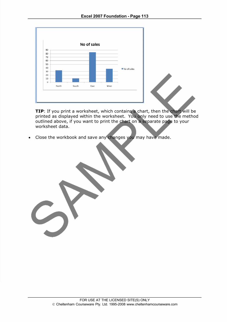
8/11/2019 Excel 2007 Foundation
http://slidepdf.com/reader/full/excel-2007-foundation 115/115
Excel 2007 Foundation - Page 113
TIP: If you print a worksheet, which contains a chart, then the chart will beprinted as displayed within the worksheet. You only need to use the methodoutlined above, if you want to print the chart on a separate page to your
worksheet data.
• Close the workbook and save any changes you may have made.