examining land reform in south africa: evidence from
TRANSCRIPT
Univers
ity of
Cap
e Tow
n
2
Examining Land Reform in South Africa: Evidence from Survey Data
JOANNA RYAN
Thesis presented for the Degree of DOCTOR OF PHILOSOPHY
In the School of Economics UNIVERSITY OF CAPE TOWN
January 2017
Supervisors: Murray Leibbrandt
Patrizio Piraino
Univers
ity of
Cap
e Tow
n
The copyright of this thesis vests in the author. No quotation from it or information derived from it is to be published without full acknowledgement of the source. The thesis is to be used for private study or non-commercial research purposes only.
Published by the University of Cape Town (UCT) in terms of the non-exclusive license granted to UCT by the author.
1
The copyright of this thesis rests with the University of Cape Town. No quotation
from it or information derived from it is to be published without full
acknowledgement of the source. The thesis is to be used for private study or
non-commercial research purposes only.
3
Acknowledgements
I am very grateful for the funding I have received, without which I would not have been able to pursue
my PhD research. I would like to acknowledge and thank the DST-NRF Centre of Excellence in Food
Security, DST-NRF Research Chair in Poverty and Inequality Research, the Carnegie Corporation, and
the No Poor Project for their generous support.
I would like to thank my supervisors, Murray Leibbrandt and Patrizio Piraino, for their continuous
advice, support, and patience. They were also both integral in securing the funding I received. My
research benefitted considerably from the different perspectives they each contributed, and I am very
grateful indeed to have had such inspiring and knowledgeable guidance.
4
Abstract
Land and land reform have long been contentious and highly charged topics in South Africa, with land
performing the dual functions of redress for the past and development for the future. This research
explores both these aspects of land, with the focus being on the impact of land receipt on household
welfare and food insecurity, and social preferences for fairness and redistribution more generally. One
of the main aims is to contribute to the land reform debate by providing previously-lacking
quantitative evidence on the aggregate welfare outcomes of land redistribution, as well as the extent
of social preferences for redistribution in the land restitution framework.
In exploring these issues, the welfare outcomes of land are first explored using the National Income
Dynamics Study (NIDS) data and unconditional quantile regression analysis. The focus is then
narrowed to the food insecurity impact of land receipt, beginning with a methodological chapter
outlining the development of a new food insecurity index applying the Alkire-Foster method of
multidimensional poverty measurement (2009; 2011). This is followed by the presentation and
discussion of food insecurity profiles of land beneficiary and non-beneficiary households. The new
index is also used as an outcome measure in exploring the determinants of household food insecurity.
These two sections again use the NIDS data. The final section shifts the emphasis from the economic
welfare benefits of land redistribution to notions of fairness and social justice encapsulated by land
restitution. A behavioural laboratory experiment is used to investigate social preferences for fairness,
and the factors that influence redistributive inclinations, by exploring the relative weights placed on
fairness considerations and self-interest, as well as the fairness ideal.
The findings indicate that beneficiaries do not use the land received for productive purposes, a
possible explanation for the limited economic welfare impacts of land reform that are observed.
Despite this limited developmental impact, the laboratory experiment makes it clear that land reform
plays an important role in addressing other needs and wants in society, particularly in respect of
preferences for fairness and addressing historical injustices.
5
Contents
Acknowledgements...................................................................................................................... 3
Abstract ....................................................................................................................................... 4
List of Tables ................................................................................................................................ 8
List of Figures ............................................................................................................................. 10
Chapter 1: Introduction .............................................................................................................. 11
Chapter 2: Locating Land Reform Research in the Policy Milieu ................................................... 16
2.1 Introduction ................................................................................................................................ 16
2.2 The Historical Context of Land in South Africa ........................................................................... 18
2.3 Land Reform Policy on Paper ...................................................................................................... 20
2.3.1 The formulation of land reform policy ................................................................................. 20
2.3.2 The White Paper on Land Reform ........................................................................................ 22
2.3.3 Land Redistribution Programmes ........................................................................................ 24
2.3.4 The Land Restitution Programme ........................................................................................ 28
2.4 Land Reform Policy in Practice .................................................................................................... 29
2.4.1 Institutional capacity constraints ......................................................................................... 30
2.4.2 South Africa’s Agricultural Legacy ........................................................................................ 31
2.4.3 Practical Implications of Policy Changes .............................................................................. 33
2.4.4 Lack of Knowledge ............................................................................................................... 34
2.4.5 Inadequate Involvement of Poor Beneficiaries ................................................................... 35
2.5 Relevance for This Research ....................................................................................................... 35
Chapter 3: Exploring the Role of Land Redistribution Policy in Household Welfare ....................... 37
3.1 Introduction ................................................................................................................................ 37
3.2 Household Welfare ..................................................................................................................... 40
3.2.1 The Dependent Variable ...................................................................................................... 40
3.2.2 The Covariates ...................................................................................................................... 42
3.2.3. Methodological concerns .................................................................................................... 44
3.3 Unconditional Quantile Regression Analysis .............................................................................. 44
3.4 Data ............................................................................................................................................. 47
3.4.1 Descriptive Statistics ............................................................................................................ 49
3.4.2 Further Descriptive Analysis ................................................................................................ 52
3.5 Regression Results ...................................................................................................................... 53
3.5.1 Replication using different data ........................................................................................... 56
3.6 Robustness Tests ......................................................................................................................... 56
6
3.6.1 Varying Bandwidths ............................................................................................................. 57
3.6.2 Quintiles ............................................................................................................................... 58
3.6.3 Alternative measures of welfare .......................................................................................... 59
3.6.4 Bootstrap Standard Errors ................................................................................................... 60
3.7 Conclusion ................................................................................................................................... 62
Chapter 4: Multidimensional Food Insecurity Measurement ....................................................... 64
4.1 Introduction ................................................................................................................................ 64
4.2 Developing the Multidimensional Food Insecurity Index ........................................................... 66
4.2.1 Dimensions, Indicators, and Cut-offs of the Index ............................................................... 67
4.2.2 Data ...................................................................................................................................... 71
4.2.3 The Indicators ...................................................................................................................... 72
4.2.4 Deprivation by Indicator Findings ........................................................................................ 77
4.2.5 Aggregation of the Indicators into an Index ........................................................................ 81
4.2.6 Using the Decomposition Properties of the Index for Food Insecurity Analysis in South
Africa ............................................................................................................................................. 83
4.3 Robustness checks ...................................................................................................................... 92
4.4 Policy Discussion and Conclusion ................................................................................................ 99
Chapter 5: Land Redistribution and the Multidimensional Food Insecurity Index ....................... 104
5.1 Introduction .............................................................................................................................. 104
5.2 Food Insecurity Profiles of Land Reform Beneficiaries and Non-Beneficiaries......................... 106
5.3 Factors Determining Food Insecurity Status ............................................................................. 117
5.4.1 Summary Statistics ............................................................................................................. 120
5.4.2 Regression Analysis ............................................................................................................ 122
5.5 Conclusion ................................................................................................................................. 124
Chapter 6: Exploring the Limits to Social Preferences for Redistribution .................................... 127
6.1. Introduction ............................................................................................................................. 127
6.2 Distributive Justice .................................................................................................................... 130
6.3 Experimental Literature on Fairness ......................................................................................... 131
6.4 Experimental Design ................................................................................................................. 133
6.4.1 The Experimental Design ................................................................................................... 134
6.4.2 Spectator Motivation: Fairness and Self-interest .............................................................. 134
6.4.3 Experimental Procedure .................................................................................................... 137
Research questions ..................................................................................................................... 144
6.5 Main Analysis and Results ......................................................................................................... 145
6.5.1 The Sample ......................................................................................................................... 146
6.5.2 Summary Statistics ............................................................................................................. 146
7
6.5.3 Logistic Regression Analysis ............................................................................................... 153
6.6 Motivations for the redistributive choices made ..................................................................... 162
6.7 Conclusion ................................................................................................................................. 166
Chapter 7: Conclusion .............................................................................................................. 170
Appendix ................................................................................................................................. 176
References ............................................................................................................................... 205
8
List of Tables
Table 3.1: Summary Statistics………………………………………………………………………………………………………….49
Table 3.2: Further Summary Statistics……………………………………………………………………………………………..52
Table 3.3: Regression Output…………………………………………………………………………………………………………..54
Table 3.4: Estimation Using Silverman’s Bandwidth…………………………………………………………………………57
Table 3.5: Estimation for Quintiles…………………………………………………………………………………………………..58
Table 3.6: The Square Root Scale……………………………………………………………………………………………………..59
Table 3.7: The South African Specific Equivalence Scale………………………………………………………………..…59
Table 3.8a: Main Results Without Accounting for the Survey Design……………………………………………….60
Table 3.8b: Bootstrap Standard Errors……………………………………………………………………………………………..61
Table 4.1: Multidimensional Food Insecurity Measures for South Africa………………………………………….85
Table 4.2: Results of Sensitivity Tests on H, A, and MFII scores for South Africa………………………………93
Table 4.3: Subpopulation Figures and Rankings for Original Weights and Cut-offs…………………………..95
Table 4.4: Cross-dimensional 3/6 Cut-off Sensitivity Results for Subpopulations……………………………..95
Table 4.5: Reweighting Subjective Measures Sensitivity Results for Subpopulations……………………….96
Table 4.6: Reweighting Anthropometric Measures Sensitivity Results for Subpopulations………………96
Table 4.7: Changing the Physical Consequences Dimensional Cut-off from 1 to 2 …………………………..97
Table 4.8: MFII Including Obesity ……………………………………………………………………………………………………98
Table 5.1: Multidimensional Food Insecurity Measures…………………………………………………………………109
Table 5.2: Summary Statistics………………………………………………………………………………………………………..120
Table 5.3: Regression Results…………………………………………………………………………………………………………122
Table 6.1: Summary of the Sample…………………………………………………………………………………………………146
Table 6.2: Average Income of Player A and Player B, by Treatment……………………………………………….150
Table 6.3: Logit Marginal Effects…..……………………………………………………………………………………………….154
Table 6.4: Elasticities of Preferences for Redistribution…………………………………………………………………156
Table 6.5: Prevalence of Fairness Views by the Initial Inequality Level…………………………………………..158
Table 6.6: Prevalence of Fairness Views by the Personal Cost of Redistribution…………………………….158
Appendix:
Table A2.1: Redistribution Figures………………………………………………………………………………………………….176
Table A2.2: Restitution Figures………………………………………………………………………………………………………176
9
Table A3.1 Correlations………………………………………………………………………………………………………………….183
Table A3.2: Estimation for Rural Households Only…………………………………………………………………………183
Table A3.3: Estimation for Urban Households Only……………………………………………………………………….184
Table A4.1: Correlation Table of Deprivation by Indicator……………………………………………………………..185
Table A5.1: Marginal Effects of Logit Regressions………………………………………………………………………….188
10
List of Figures
Figure 4.1: Structure of the Multidimensional Food Insecurity Index……………………………………………….70
Figure 4.2: Provincial Deprivations by Indicator: Anxiety and Uncertainty……………………………………….78
Figure 4.3: Provincial Deprivations by Indicator: Insufficient Quality……………………………………………….79
Figure 4.4: Provincial Deprivations by Indicator: Physical Consequences…………………………………………80
Figure 4.5: National Intensity of Deprivation……………………………………………………………………………………86
Figure 4.6: Indicator Contributions to National MFII………………………………………………………………………..87
Figure 4.7: Provincial Contributors to the National MFII………………………………………………………………….88
Figure 4.8: Urban and Rural Contributors to the National MFII………………………………………………………..88
Figure 4.9: Provincial Food Insecurity………………………………………………………………………………………………89
Figure 4.10: Indicator Contributions to MFII Score by Province……………………………………………………….90
Figure 4.11: District Council MFII…………………………………………………………………….……………………………..101
Figure 5.1: Deprivation by Indicator……………………………………………………………………………………………….107
Figure 5.2: Intensity of Deprivation of the MFII Food Insecure……………………………………………………….111
Figure 5.3: Indicator Contributions to MFII…………………………………………………………………………………….113
Figure 5.4: Provincial MFII Heat Maps……………………………………………………………………………………………115
Figure 6.1: Proportion of Decisions to Redistribute ……………………………………………………………………….147
Figure 6.2: Proportion of Decisions to Redistribute at each Cost Level…………………………………………..148
Figure 6.3: Proportion of Decisions to Redistribute at each Initial Inequality…………………………………149
Figure 6.4: Resultant Inequality……………………………………………………………………………………………………..151
Figure 6.5: Resultant Inequality by Cost…………………………………………………………………………………………152
Figure 6.6: Survey Question 12………………………………………………………………………………………………………160
Figure 6.7: Survey Question 13………………………………………………………………………………………………………161
Figure 6.8: Survey Question 14………………………………………………………………………………………………………161 Appendix:
Figure A4.1: The Proportion of the Food Insecure Deprived on Each Indicator………………………………186
11
Chapter 1: Introduction
Internationally the case for redistributing land is argued to be strong, especially in countries with a
highly unequal distribution of land. There are several key elements to the case, including conflict
prevention, equity, economic growth, jobs, and poverty reduction (Binswanger-Mkhize, Bourguignon
& van den Brink, 2009). In South Africa land and land reform have long been contentious and highly
charged topics, spanning political, economic, and social discourses. In 2017, more than 22 years since
the end of apartheid, the topic is gaining increasing traction and attention. There are a few reasons
for this, largely stemming from general dissatisfaction and frustration with the slow progress of
economic reform in South Africa, and the unacceptably high level of interracial inequality that is a
feature of this lack of progress.
Recently the land issue has been reignited, largely headed by the Economic Freedom Fighters (EFF)
led by Julius Malema, with strong calls for redistribution without compensation, as well as black
occupation of vacant, white-owned land. Malema has recently been accused of racism and inciting
violence with his public statements that all black people wanted was their land back, and that “we are
not calling for the slaughtering of white people ... at least for now” (Madia, 2016), as well as “we will
take our land no matter how. It’s becoming unavoidable, it’s becoming inevitable” (Madia, 2016).
Increasing popular support for these strong ideological positions on land likely reflects the appeal of
the calls, which incorporate both the economic value of land, as well as the unfairness in racial land
ownership patterns resulting from the forced land removals of apartheid and British colonialism.
These impassioned and contentious statements and positions on land reflect how important and
emotional the land issue is.
But how well-founded is the demand for land as a means of economic liberation? At present, there is
near-consensus that land reform in South Africa has been unsuccessful, even as the debates and
vociferous calls for action persist (Aliber & Cousins, 2013). There is however very little in the way of
quantitative evidence to either support or refute the various claims made. Currently the progress and
success of land redistribution and restitution are measured in terms of the number of hectares
redistributed, the number of claims settled, and the total number of beneficiaries. Less attention is
paid to the welfare outcomes of those who receive land, and the notion that land translates into
improved welfare is simply assumed rather than tested.
There are two important concepts to be distinguished when considering the outcomes of land reform
policy, aptly put as the ‘twinned but incongruent imperatives of redress for the past and development
for the future’ (Walker, 2005). Redress for the past refers to the restitution aspect of land reform that
12
addresses racially-based land dispossessions of the past. Development for the future concerns the
economic and livelihoods aspect of land reform as tackled by land redistribution. While various survey
studies indicate that access to land and land reform policy for the purposes of economic activity may
not be priorities, the important role played by land as a tool for redress is widely acknowledged.
In studying the outcomes of land reform policy this research explores the productive and welfare
function of land, as well as the role of land from the social justice and fairness perspective. More
specifically the work focusses on household welfare and food insecurity in the context of land
redistribution, as well as investigating social preferences for fairness and redistribution more
generally. One of the main aims is to contribute to the land reform debate by providing quantitative
evidence on the aggregate welfare outcomes of land redistribution, as well as the extent of fairness
considerations and social preferences for redistribution in the land restitution framework. Various
approaches are employed in exploring these issues, including the analysis of a nationally
representative data set, the development of a new food insecurity index, and a behavioural laboratory
experiment.
The first section of the thesis serves to set the scene for the analyses by detailing the development
and evolution of land redistribution and restitution policy in South Africa. Land reform policy is
complex to navigate, and a thorough outline of the various aspects of the programmes involved, and
the numerous updates and revisions to aims, eligibility and implementation is necessary. The
intricacies of the policy are important to be aware of and understand as it is likely that this complexity
has had an impact on the efficacy of the various programmes. The historical context of land ownership
patterns is also discussed, providing important details about land dispossession, and underlining the
importance of land redistribution and restitution policy under these circumstances.
Following the overview of the policy milieu, the core of the thesis begins with a general investigation
into the relationship between land redistribution and household welfare. This chapter exploits a
nationally representative survey, conducted in 2014 and 2015, to explore the impact of land receipt
and subsistence farming on household welfare. The South African government and other stakeholders
maintain that land reform is a priority for rural development, with household agriculture being the
mechanism through which the policy translates into improved household welfare. However, a review
of the policy implementation environment and academic literature raises questions about the
programme and its efficacy. The appropriateness of land reform is questioned in various respects,
including the perception that South Africans are no longer interested in pursuing an agrarian lifestyle,
and the significant input costs required for productive land use.
13
While much has been written about the role of land reform and household welfare, there is little in
the way of empirical evidence. This chapter explores land beneficiary household characteristics, and
the role that the receipt of land plays in the welfare of these households. The impact of access to land
and household agricultural activity are also examined as associated, yet distinct, indicators.
Unconditional quantile regression analysis is used to determine the impact of these key variables at
various quantiles of the household expenditure distribution. The results indicate that the receipt of
land persistently does not have a significant relationship with household welfare, and the influence of
agricultural involvement and access to land is limited. While it is acknowledged that regression
analysis may not be the most suitable method to address this question, the exercise makes use of the
limited nationally representative data on land redistribution that is available, making for a unique
empirical land study. It also proves a useful starting point from which to broach the topic of the
relationship between land and welfare outcomes, and discuss some of the concerns and issues that
are revealed.
Chapters 4 and 5 narrow the scope from household welfare in general to focus specifically on
household food insecurity, and in what ways land redistribution might be having an impact. Access to
land is often considered a determinant of involvement in agriculture, one argument being the
potential increase in own-production if resources, and more specifically access to land, are improved
(Altman, Hart & Jacobs, 2009). This notion that increased access to land translates into increased
production is not often interrogated in the literature, particularly in an empirical manner. The
assumption that this process is occurring should not be made lightly, as it is a critical link in the
realisation of any benefits from the land redistribution programme. Despite the various changes in
land redistribution policy, household food security has consistently featured prominently as a core
goal. Little is known about the aggregate impact that land redistribution is having on beneficiaries,
and examining household food insecurity is a quantifiable and relevant measure of how it might be
improving livelihoods.
That said, it is well established that food security is a complex phenomenon with numerous indicators
and outcomes, the measurement of which are yet to be adequately captured by a single measure. As
such Chapter 4 outlines the development of a comprehensive measure of food insecurity. The
adoption of the methodology of multidimensional poverty measurement is proposed in calculating an
index of multidimensional food insecurity. This framework has gained increasing popularity,
particularly with the introduction of the Multidimensional Poverty Index (MPI) (Alkire & Santos, 2010).
The assertion is that, like poverty, food insecurity is a multidimensional phenomenon, requiring the
inclusion of multiple aspects of deprivation in its measurement. Nationally representative data from
14
South Africa is used to construct a Multidimensional Food Insecurity Index (MFII), based on the
methodology of the MPI. This MFII is then used to develop a detailed profile of individual food
insecurity in South Africa. Nationally, close to half the population are considered multidimensionally
food insecure, with the greatest contributors to food insecurity being poor dietary diversity and
subjective food consumption inadequacy. The Western Cape and Gauteng enjoy the lowest levels of
multidimensional food insecurity, while Limpopo and KwaZulu-Natal suffer the highest levels.
Following the development of the MFII the focus in Chapter 5 returns to the issue of land and food
insecurity, and the index is used as a measurement tool in the land redistribution framework. A
detailed descriptive profile of food insecurity of land beneficiary and non-beneficiary households is
presented first. From this descriptive characterisation there does not appear to be any meaningful
difference in the food insecurity levels of the two groups. In general, land redistribution beneficiaries
do however have a slightly higher MFII score than non-beneficiaries, and suffer greater severity in
food insecurity. The analysis is then broadened to consider what factors in addition to the receipt of
land may have a significant bearing on food insecurity status. Using a welfare model similar to that
outlined in Chapter 3, linear probability regression analysis reveals that neither obtaining land through
land redistribution, nor being involved in agriculture, has a significant influence on a household being
food insecure or severely food insecure. Factors that are relevant include rural location, employment
levels, the proportion of adults in the household, and household head characteristics such as age and
education level. The findings reflect those from the household welfare investigation in Chapter 3, with
the redistribution of land seemingly having a limited influence, if any, on food insecurity.
As stated at the outset, land serves more than just an economic purpose, and the role played by land
restitution as redress for past injustices and the promotion of fairness is arguably as important in the
South African context. Fairness is stated as one of the key elements of the case for land redistribution,
with history, culture, and a few other factors moulding what a society thinks is fair use and ownership
of land (Binswanger-Mkhize, Bourguignon & van den Brink, 2009). While it does not appear that land
is achieving the economic aims hoped for, it is generally acknowledged that the land restitution
process plays a crucial role in addressing the arbitrary and unfair land dispossessions of the past.
Chapter 6 shifts the emphasis from the economic welfare benefits of land redistribution, to the
notions of fairness and social justice encapsulated by land restitution. The focus of this chapter is not
specifically on land, but rather societal preferences for redistributive justice, which extend beyond
land. Using an economic experiment based on the theoretical model of Cappelen et al (2007; 2013),
the final chapter explores social preferences for fairness, and the factors that influence redistributive
15
inclinations. Distributive justice can be defined as the perceived fairness of how rewards and costs are
shared by group members. To determine what distributive justice is, individuals often turn to the
distributive norms of their group which are comprised of individual fairness ideals, and the weight
placed on fairness and self-interest. This chapter uses an economic experiment to explore what these
distributive norms might be, as well as the relative weights placed on fairness considerations and self-
interest, and the fairness ideal. By varying the size of the initial income inequality, the weight placed
on fairness considerations and the fairness ideal are tested, and by increasing the personal costs of
redistribution, the self-interest motivation is investigated. The impact of the source of the inequality,
in terms of luck or merit, is also explored.
The findings indicate greater aversion to higher initial inequality, resulting in more redistribution
occurring when inequality levels are high. Aversion to inequality is mitigated by increasing personal
cost, resulting in less redistribution occurring at higher costs. The source of the inequality also matters,
with the effects of cost being greater in the Merit treatment compared to the Luck treatment. In
general, the results indicate an aversion to inequality and a robust willingness to redistribute,
particularly when inequality is high and the source is unfair. The willingness to redistribute is however
curtailed by the personal cost involved, with little redistribution taking place at high costs.
There is no doubt that land is a highly-charged and contentious issue in South Africa, and one that is
increasing in prominence. In the face of the sometimes-combative debate, there is an urgent need for
quantitative evidence to guide policy. In providing such evidence, this research begins with a
discussion about the history and context of land reform policy, followed by four core chapters, and is
structured as follows: Chapter 2: Locating Land Reform Research in the Policy Milieu; Chapter 3:
Exploring the Role of Land Redistribution Policy in Household Welfare; Chapter 4: Multidimensional
Food Insecurity Measurement; Chapter 5: Land Redistribution and the Multidimensional Food
Insecurity Index; and Chapter 6: Exploring the Limits to Social Preferences for Redistribution. Chapter
7 concludes.
16
Chapter 2: Locating Land Reform Research in the
Policy Milieu
2.1 Introduction
There are usually multiple justifications for land reform, including unequal distribution of land and
extensive rural poverty, both of which are particularly relevant in the South African context. In most
cases however, including in South Africa, the primary motivation for land reform has been political
rather than economic (Deininger, 2003). This has resulted in a short-term focus on quick reforms, with
little emphasis placed on increasing agricultural productivity and improving welfares.
As a result of the racial segregation of apartheid in South Africa, land as a right is a historical construct.
Land is also a resource, which can facilitate the realisation of other rights, such as housing and
subsistence farming (Aliber, Reitzes & Roefs, 2006). These two characteristics of land, as a right and
as a resource, are the focus of land reform in South Africa. The Policy Framework document of the
Reconstruction and Development Plan (RDP) first articulated the process of land reform as the central
and driving force of a programme of rural development (ANC, 1994). It specified that there should be
three main elements of land reform aimed at addressing the rights and resource aspects of land:
1. Land redistribution: where people apply for assistance with which to acquire land for farming and/or settlement
2. Land restitution: the restoration of land or other compensation to victims of forced removals
3. Tenure reform: improves the clarity and robustness of tenure rights, mainly for residents of former homelands
These three aspects are included in the Bill of Rights of the Constitution and remain the basis for
current land reform policy (Constitution of the Republic of South Africa, 1996). The National
Development Plan 2030 Chapter 6 entitled “An Integrated and Inclusive Rural Economy”, echoes the
RDP emphasis, detailing successful land reform as the basis for the agricultural development plan,
with a focus on smallholder farmers (National Planning Commission, 2012).
Land reform in South Africa is a complex and evolving process, which has thus far been criticised for
not delivering on ambitious promises of land and agrarian reform. The policy milieu is complicated to
navigate due to various factors, including the historical context, the changing policies and departments

17
involved, and the disjuncture between policy in theory and the implementation in practice. Evaluating
land reform is an extensive topic, necessitating a well-defined research agenda with narrow questions
to define and limit the scope. This first contextual chapter is focused on specific aspects of land reform
that will serve to lay the groundwork for the following chapters. The discussion focuses on the land
redistribution and restitution arms of land reform, specifically beneficiaries and the welfare impact of
the various implementation programmes of the policy. The third arm of land reform, tenure reform,
is not considered directly for largely practical reasons. Tenure reform refers to security of tenure for
labour tenants, the upgrading and conversion into ownership of certain rights graded in respect of
land, as well as for the transfer of tribal land in full ownership to a tribe. Specifically, this includes lease
hold on state and public land, private land free hold with limited extent, foreign land ownership, and
communal land tender (DRDLR, 2016). Tenure reform does not necessarily refer to land changing
hands, but more to the rights of access to land, and it is not always clear who the beneficiaries are or
in what way they benefitted. More importantly for this research there is very little data, if any, that
can be used as an indicator for tenure reform beneficiaries. For example, in the Department of Rural
Development and Land Reform 2015/2016 annual report there are no statistics supplied relating
specifically to tenure reform - not from the beneficiary, department, or financial perspective (DRDLR,
2016).
What the role of land might be in South Africa is a complex question with several sub-contexts. These
can be broadly grouped into the rights and resources aspects of land mentioned previously. Land is
used as a tool to address injustices of the past and is highlighted as a right in the Constitution. It is also
the key resource tasked with tackling rural poverty and household food insecurity. Within the
resources context of land there exists some disjuncture in how the successes and achievements of
land redistribution are measured (Walker, 2005). The redistribution targets set by the Department of
Rural Development and Land Reform (DRDLR) focus on the amount of agricultural land that needs to
be transferred to black beneficiaries, rather than any measure of improved livelihood or food
insecurity.1 The department releases performance target figures based on the number of hectares
transferred and the number of beneficiaries. For the twenty years since inception in 1994 to 2014,
4 313 169 hectares of land has been redistributed to 233 289 beneficiaries from 122 010 households.2
The most recent 2017 figures indicate that a total of 4 850 100 hectares have been redistributed
(Sihlobo & Kapuya, 2017). In reporting performance there is no mention of how livelihoods have
improved or the number of households with increased food security. A concern is that many land
1 The initial target was 30 percent of white-owned land redistributed over a period of 5 years 2 Detailed DRDLR land reform figures can be found in Appendix A2.1

18
reform projects have not been successful, resulting in unproductive land and little change in
beneficiary welfare. Measuring land redistribution in terms of the number of beneficiaries and
hectares transferred gives no indication of the real impact that the programme is having. With respect
to the restitution programme, performance is also measured and reported as the number of claims
that have been settled.3
The general failure of land reform to date is recognised, with proponents of land reform focussing on
the potential of the programmes. This potential of land redistribution to achieve its goals of agrarian
reform and rural poverty alleviation is however contested, with some cautioning that subsistence
agriculture through land redistribution is neither a suitable nor sustainable route to follow in South
Africa. This is largely due to shifting values and perceptions of land-based livelihoods in that they are
not considered desirable by a growing number of those in rural areas, especially the youth (Ntsebeza,
2010). Thus, there is some concern regarding an apparent limited demand for land (Lahiff & Li, 2012;
CDE, 2005). This review of land reform policy will begin by briefly examining the historical context of
land dispossession in South Africa, followed by land reform policy on paper and in practice. This
includes the policy development process and the evolution of the redistribution implementation
programmes.
2.2 The Historical Context of Land in South Africa
Prior to discussing land reform policy, it is important to have an understanding about the historical
context of land in South Africa. While not attempting to articulate all the historical details of land
dispossession, a brief overview will provide the necessary background in which to locate current land
reform policy.4 Although 1913 has been chosen as a landmark year for restitution claims, land
dispossession and forced removals were in practice long before then. Until 1994 the dispossession of,
and forced removal from, land was a tool used extensively in South Africa to control and suppress the
majority black population.5 In the 19th century British colonial conquest was accelerated resulting in
the voortrekkers6 moving out of the Cape Colony to escape British rule. As they travelled inland they
fought, seized, and dispossessed black communities of their land. The British in turn pursued the
3 Detailed DRDLR land restitution figures are in Appendix A2.1 4 For a detailed account of events see Bundy, 1988, & Wilson, 1971. 5 Black is taken to mean non-white rather than African 6 The Afrikaans pioneers who left the Cape during British colonial rule
19
voortrekkers, appropriating more land and claiming back other land from the voortrekkers. The
mineral revolution which boomed in the 1800’s also contributed to land dispossession as the white
colonial government sought to force Africans off their land to become cheap labour in the newly
established mines (SA History, 2014).
By the early 20th century colonial rule was being entrenched, with numerous pieces of legislation
passed to uproot native people from their land and prevent them purchasing land in certain areas. On
17 June 1913, the Native Land Act was passed, and The Native Land Commission7 was established to
find land and determine borders across the country for territorial segregation between black and
white people. The commission submitted its report in 1916, outlining which areas were to be allocated
to white people and which areas to black people. Initially the land allocated to black people amounted
to 7% of the total land area of South Africa, and in 1936 this area was increased to 13.6%. In 1923 the
Natives (Urban Areas) Act was passed, allowing urban authorities to establish ‘locations’ where black
people working in urban areas were to live. Land in these locations was never owned by black people,
but only occupied by them. While numerous acts aimed at controlling the movement and settlement
of black people were passed, the 1913 Native Land Act is considered the defining piece of legislation
that formalised land ownership patterns established many years before (Jooste, 2013).
The displacement of African people coincided with the introduction of European agricultural practices
that were both poorly suited to South African soil and climate patterns, and caused a shift away from
traditional migrant pastoral farming behaviour (Jooste, 2013). African tribes traditionally adopted
seasonal, expansive, pastoralism-dominated methods of food production because of the varying
rainfall patterns and agricultural capacity of different regions in South Africa. The prime agricultural
land, cheap labour, trade resources, and settlement patterns demanded by colonisation restricted
African individuals to small patches of land on which to farm, and forced the breakdown of the family
agricultural unit (Jooste, 2013). During the colonial period not only did African people lose their land,
but also their traditional farming way of life.
The rise of the National Party to power in 1948 led to the entrenchment of the colonial segregation of
black and white people, with further legislation isolating black people from their land and property.
The Group Areas Act passed in 1950 allowed for the forced removal of black people from declared
white areas, and expelled them to self-governed ‘homelands’ that had been established in rural areas.
Prior to the democratic elections in 1994 discussions and efforts were underway to address issues of
land and settlement. The 1913 and 1936 Land Acts were revoked in 1991 by F.W. De Klerk through
the enactment of the Abolition of Racially Based Land Measures Act and the Upgrading of Tenure Act
7 Also known as the Beaumont Commission
20
(SA History, 2014). The development of current South African land reform policy followed from these
first steps.
2.3 Land Reform Policy on Paper
2.3.1 The formulation of land reform policy
The process of formulating land reform policy began in the late 1980s in the run up to the 1994
democratic elections. While a number of stakeholders were involved, a glaring omission was the rural
poor. This is despite the fact that the rural poor - comprising victims of land dispossession, small-scale
farmers, farm workers, labour tenants, communal area residents, women, and youth - were to be the
primary beneficiaries (Cousins, 2016). It has been argued that policy formulation and the nature of
subsequent policy implementation programmes, are the outcomes of the distribution of power within
the society in question, as well as globally (Weideman, 2004). This is reflected in the major players
that influenced land reform policy, including the National Party, the World Bank, the African National
Congress (ANC), rural and land-related NGO’s, the National African Farmer’s Union, the white
commercial agricultural sector, the former department of Native Affairs, and the (then) new
departments of Agriculture and Land Affairs. As a result of the influence of these groups, and the lack
of representation of poor beneficiaries, the policy developed is a three-part, demand-driven, market
based programme (Weideman, 2004). Indeed, it can be argued that the policy design largely maintains
the status quo of land, without the necessary means and motivation to radically change the face of
agriculture and land in South Africa (Levin and Weiner, 1996; Bond 2000; Weideman 2004; Cousins
2013 & 2016; Hall, 2009 & 2013).
The National Party (NP) introduced its White Paper on Land Reform in 1991. Regarding redistribution,
the NP specified that this would take place within a free market context. This refers to the willing
buyer willing seller framework within which land transfer takes place. At the time, opponents argued
that addressing the land injustices and achieving equity in land ownership required a state-led
intervention because the poor did not have the resources to participate in the free market.
Furthermore, it was argued that such policies entrenched the social and economic inequalities of
apartheid (Weideman, 2004).
21
The position of the NP was supported by the recommendations of the World Bank’s representatives
who argued for a market-based land reform programme. Several other key aspects adopted in the
policy were also because of World Bank recommendations. These include the liberalisation of
agriculture and the abolition of protectionist agricultural policies, a constitutional guarantee of
protection of property rights, a three-part programme separated into restitution, redistribution, and
tenure reform, and the initial timeframe and land transfer objectives.
By 1990 the ANC had not developed any concrete land and agrarian reform policies, and these issues
had not featured on the ANC agenda. The real work began in the early 1990’s, and at an ANC land
conference nationalisation was a dominant theme, while issues such as regulated land markets,
sharecropping, the development of a black commercial agricultural sector, and safety nets for the poor
were mentioned. These last two issues have been reflected in the various implementation arms of
land policy. But these processes were not coordinated and, as a result, the ANC has been accused of
not being interested in the land reform policy development process, resulting in a policy largely
reflecting the interests of the elite (Weideman, 2004).
The white commercial agricultural sector was naturally interested in maintaining the existing state of
affairs regarding land. While committed to negotiations, the sector supported the willing buyer willing
seller principle, and emphasised the importance of providing support services to new farmers. This
issue of post-settlement assistance has turned out to be a notable weakness in the implementation
process due to the inadequacy of support services. Furthermore, the current focus on the
development of a black commercial farming sector closely resembles the arguments proposed by the
white agricultural farming sector in the 1990’s (Weideman, 2004).
The National African Farmer’s Union (NAFU) was founded in the 1990’s partly in response to the lack
of representation of commercial and established black farmers in the initial policy development
process (Weideman, 2004). The shift in policy focus in early 2000 from poverty alleviation to the
development of a class of black commercial farmers has been attributed to some extent to the efforts
of NAFU. While late to the party, NAFU managed to have a real impact on land reform policy to the
benefit of black commercial farmers.
The rural poor and landless, who were not represented in the initial policy process, have still not
participated meaningfully in policy formulation and implementation. This lack of representation has
played out in the shift in focus away from alleviating poverty and assisting the truly poor in accessing
land, to a system of land reform policy that favours black commercial farmers. The initial promise of
redistributed land being used for smallholder farming is not being supported in practice (Cousins, 2016
& 2013; ARI, 2013).
22
2.3.2 The White Paper on Land Reform
Chapter 2 of the Constitution of the Republic of South Africa outlines the Bill of Rights which forms a
cornerstone of democracy in South Africa. Section 25 focuses on property rights, and highlights the
role of land reform in ensuring this right to property (Constitution of the Republic of South Africa,
1996). While it guarantees property rights, it simultaneously outlines the duty of the state to take
reasonable steps to enable citizens to gain equitable access to land, promote security of tenure, and
to provide redress to those dispossessed of property.
The constitutional right to land, and the role of the state in ensuring this right, are articulated in the
1997 White Paper on Land Reform (DLA, 1997). The White Paper details the purposes and
implementation of land policy, largely divided into the three areas of restitution, redistribution, and
tenure reform. The case for land policy, as outlined in the White Paper, is stated as being four-fold
(DLA, 1997):
o To redress the injustices of apartheid;
o To foster national reconciliation and stability;
o To underpin economic growth; and
o To improve household welfare and alleviate poverty.
In line with this, there are a few economic arguments for land reform proposed in the White Paper,
two of which are going to be examined in the core chapters of this research:
More households will be able to access sufficient food on a consistent basis: access to
productive land will provide opportunity for putting more food on the table and providing
cash for the purchase of food items.
Opportunities for small scale production: small scale and subsistence farmers could be
assisted by the land redistribution programme to expand their resource base through land
purchase or lease.
Regarding land redistribution, the purpose is to provide the poor with land for residential and
productive purposes to improve their livelihoods. The target groups are the urban and rural poor, farm
workers, labour tenants, and emergent farmers. Within these groups, women and the marginalised
will be given priority.
In terms of accessing a land redistribution grant, the White Paper notes that communities often
experience problems gaining access to information about land development opportunities and
23
processes. In addition, communities are not able to express a realistic demand for land.8 These are not
trivial issues as the land redistribution programme is demand driven, relying on considerable effort on
the part of potential beneficiaries to access the grant. There are two proposals aimed at addressing
the access to information problem, the first being the role of the Post Office as a centre in rural areas
providing information on government grants. The second proposal involves the state making funds
available for the employment of information agents by rural organisations (DLA, 1997). These
initiatives are not currently in place, and it is doubtful whether they ever were implemented.9 There
do not appear to be any proposed solutions to the issue of the inability to express a demand for land.
The role played by the Provincial Department of Land Affairs (now the Department of Rural
Development and Land Reform, DRDLR) is highlighted as being key to effective and efficient
implementation of land reform, with regional offices being the front-line of land reform delivery. The
division of activities between the regional offices and provincial authorities is however not defined
beyond stating that this will vary according to negotiated arrangements, and conditions specific to the
province. The implementation details of land reform policy remain province-specific, with district and
local offices employing different application and land allocation criteria.
The Subdivision of Agricultural Land Act 70 of 1970 is mentioned numerous times in the White Paper,
and most significantly the waiving of this act for the implementation of effective land reform (DLA,
1997). It has been argued however, that a failure to implement subdivision of large farms has been
significant in the generally poor performance of land redistribution (Cousins, 2013; Hall, 2009). This
will be discussed further in later chapters.
A comprehensive overhaul of land policy and legislation as outlined in the 1997 White Paper is
currently underway, however it has stalled at the Green Paper stage. The focus of the Green Paper on
Land Reform, published in 2011, is on a ‘four tier’ tenure system, comprising: leasehold on state land;
free-hold with ‘limited extent’ (i.e. restrictions on land size); ‘precarious’ freehold for foreign land
owners (i.e. with restrictions); and communal tenure (Cousins, 2016). This brief, eleven-page Green
Paper has been accused of “fudging the important questions” (PLAAS, 2011; pp 3), including the
following:
• It fails to provide an honest analysis of the nature and shortcomings of land reform policy until
now.
8 Section 3.8.1 9 Personal interview with representatives of the Western Cape DRDLR
24
• No guidance is given as to how the state will acquire land for acquisition.
• No answer is given on the status of the ‘willing buyer, willing seller’ model.10
• No clarity is given as to when, and under what conditions, will the state use expropriation as
a way to acquire land.
• No clarity is given on how women’s rights to land can be secured.
• No useful guidance is provided as to how the implementation of land reform is to support
sustainable livelihoods.
At this stage, it does not appear that government is intending to publish an expanded version of this
Green Paper, or a comprehensive new White Paper (Cousins, 2013; 2016). Government has instead
signed off on several bills and policy documents, for example the Land Expropriation Bill and the
reopening of land restitution claims (which will be discussed), with no public debate or discussion of
these planned (Cousins, 2013).
2.3.3 Land Redistribution Programmes
The 1997 White Paper outlines the key implementation programme of land redistribution, the
Settlement/Land Acquisition Grant (SLAG), with subsequent changes to implementation programmes
being made outside of the White Paper (DLA, 1997). Since inception there have been four distinct
programme changes in the redistribution of land, from the initial Settlement/Land Acquisition Grant,
to Land Redistribution for Agricultural Development (LRAD), to the Proactive Land Acquisition Strategy
(PLAS) and the Recapitalisation and Development Programme (RADP). Each of these programmes has
different eligibility criteria, application processes, benefits in respect of land access, and goals. A
common feature is that the application process requires considerable effort, capabilities, and
knowledge on the part of applicants.
SLAG was the first land redistribution programme introduced in 1994, and was characterised as
directly targeting the poorest of the poor, as indicated by the household means test, which was done
with some success (Lahiff and Li, 2012). The programme also resembled the approach proposed by
the World Bank of market-based and state-assisted purchases of land (Hall, 2013). Individuals or
groups could apply for the grant, where the average household income for the group could not exceed
R1 500. While the grant was awarded to an individual, in effect it was a household grant, as only one
10 This has since been addressed by the new Expropriation Bill, a discussion of which is to follow
25
per household was allowed and the eligibility criteria were at the household level. The upper limit of
the grant was set at R16 000 per qualifying person (household), but the amount awarded was
dependent on the decision of the Provincial Director of the Department of Land Affairs (DLA, 1997).
The application procedure was an involved process, requiring considerable effort and resources on
the part of potential beneficiaries. The application procedure included a farm and project proposal
comprising a land use proposal, a rough cash flow projection, settlement models and patterns, and
intended agricultural use of land (DLA, 1997). Applicants were responsible for purchasing suitable land
for sale in the market using the grant money, however until the grant was actually awarded, the
applicant would generally not have been in a position to make an offer to purchase land. Nonetheless,
suitable land should have been identified and affordability assessments conducted to determine what
share of the grant would go to land purchase, what share to input and infrastructure costs, and how
much might be required as an own contribution to the project. All of this would need to have been
outlined in the application package. The maximum grant amount of R16 000 often necessitated that
beneficiaries formed groups and pooled their resources to acquire the sizable farms available on the
market. While SLAG was scaled down during the implementation of LRAD, it ceased to exist completely
in 2009 following the introduction of PLAS.
LRAD was introduced in 2001 and largely replaced SLAG as the primary land redistribution
implementation programme. While SLAG implementation did continue for settlement, the agricultural
component was largely implemented under the auspices of LRAD. The grant was provided to black
South Africans to access land specifically for agricultural purposes, with one of the strategic objectives
being the improvement of nutrition and incomes of rural poor who are interested in farming on any
scale. This description fails to capture the shift in emphasis away from assisting the poorest in
accessing land in favour of creating a class of commercial black farmers (Hall, 2013). A notable
demonstration of this shift was the removal of the R1 500 means test. By removing this means test,
the one area of the policy that was successful in targeting the poor and ensuring that benefits were
not appropriated by well-off beneficiaries, was eliminated (Hall, 2013).
LRAD, like SLAG, was demand driven meaning that beneficiaries decided on the piece of land
purchased and the scope of the project. The grant value ranged from R20 000 to R100 000 and, unlike
SLAG, required an own-contribution from beneficiaries to access the grant. The own contribution
increased relative to the grant amount applied for, and ranged from R5 000 for a R20 000 grant, to
26
R400 000 for a R1 000 000 grant. This own-contribution could take the form of cash or work in kind.11
Grants could be used to purchase land, and/or for infrastructural and production development. While
men and women were to be granted equal access to all benefits, women and youth were to be actively
encouraged to apply for the grant. Previous beneficiaries of SLAG were eligible for a LRAD grant,
although preference would be given to first-time applicants.
As with SLAG the application process involved several steps to be taken by hopeful beneficiaries.
Applicants were to select the size of the grant they would like according to their chosen own-
contribution, and identify a suitable piece of land and enter a contingent contract with the seller
(contingent on approval of the project under LRAD). Applicants were then to prepare a farm plan or
land use proposal, indicating the intended agricultural use of the land and projected cash flows, and
obtain evidence of additional financial resources, such as loans or own resources. Applicants were
obligated to submit all the required documentation to the local agricultural officer who would provide
an opinion on the feasibility of the project, as well as the suitability of the selling price of the land.
Following this, the applicant would submit the proposal package to the provincial grant committee,
comprising officers of both the departments of Agriculture and Land Affairs. Applicants could apply
individually or as a group to increase the amount of the grant applied for.
An interesting point to note about the LRAD programme is that it closely resembles the redistribution
subsidy scheme of the Department of Regional Development and Land Affairs, finalised less than 4
months prior to the first democratic elections in 1994. This scheme enabled black people to purchase
land with an 80% subsidy, a 5% contribution from the beneficiary, and a 15% loan (Hall, 2013).
PLAS is the implementation strategy that has been employed by the DRDLR since 2007, and together
with the RADP, has largely replaced the previous redistribution programmes. Together these current
strategies represent a fundamental shift away from the demand-driven nature of the grant-based
policies of the past. As the name implies, the Proactive Land Acquisition Strategy emphasises a more
active role on the part of government in obtaining land for redistribution. While potential beneficiaries
still need to indicate their demand for agricultural land by applying to enter the programme, the
identification and acquisition of suitable land is the responsibility of provincial government rather than
beneficiaries. The PLAS process is as follows: the state obtains land suitable for agriculture; applicants
complete a questionnaire and are entered into the database12; a rigorous matching process is
11 Meaning beneficiaries work on the project without drawing a salary until the contribution requirement has been met 12 The Western Cape DRDLR questionnaire can be found in Appendix A2.2
27
employed to allocate state acquired land to suitable beneficiaries in the database; successful
beneficiaries initially lease the land from the state, with an option to purchase after a specified period
of successful production (DLA, 2007).
PLAS targets black people, groups that live in communal areas and black people with the necessary
farming skills in urban areas, and people living under insecure tenure rights. Eligibility is broad, with
the programme catering for black South Africans not employed by the state, including households
with limited access to land; as well as established small and large black commercial farmers and
financially capable aspirant black commercial farmers (Hall, 2013). The pro-poor aspect of PLAS
indicates that poor people should be given preference in relation to government-aided schemes,
resulting in increased benefits for poor people. In this regard three types of poor people are identified,
with varying degrees of additional benefits such as discounts on lease fees and purchase prices
following the lease period. Since 2011 however, the option to purchase has been ruled out following
wide-spread non-payment of rent, with further promises to remove beneficiaries who are not utilising
the land in accordance with the agreed business plan (Hall, 2013). The current redistribution
programme assists in the purchasing of agricultural land by black people, but it does not in any way
support agrarian reform as articulated in the founding land reform policy. The programme has also
been criticised of returning to the old idea of conditional tenure, with unsuccessful renting
beneficiaries being removed and replaced with new beneficiaries (Hall, 2013).
The RADP is implemented in conjunction with PLAS, and is closely aligned with chapter 6 of the
National Development plan 2030 in proposing a revised plan for land reform. It is a strategic farmer
support policy, seeking to provide black emerging farmers with the social and economic infrastructure
and basic resources required to run successful agricultural businesses (DRDLR, 2013). The policy
targets properties acquired since 1996 through the various land reform programmes, including SLAG,
LRAD, and PLAS. As such, the policy does not assist applicants in obtaining land through redistribution,
but rather aids those who have already received land through the various programmes. More
specifically, land reform properties in distress and properties selected by District Land Reform
Committees are eligible for the programme, as well as sites within former homelands and other
communal areas, and farms acquired by individuals or groups from historically disadvantaged
communities. The support provided includes mentorship, co-management, share-equity
arrangements, and contract farming and concessions. The overall goal of the policy is social cohesion
and development, and is aligned with the goals of the National Development Plan 2030. The goals
most impacted by the RADP include sustainable land reform, improved food security, smallholder
28
farmer development and support, and growth of sustainable rural enterprises and industries. PLAS
and the RADP form the primary implementation arms of the Comprehensive Rural Development Plan
(CRDP). The CRDP, adopted in 2009, was conceptualised by the Department of Rural Development
and Land Reform. It forms the basis of the policy trajectory of the DRDLR, and is based on a pro-active
participatory, community-based planning approach to rural development.
2.3.4 The Land Restitution Programme
The Commission on Restitution of Land Rights and the Land Claims Court are tasked with the
restitution of rights in land following land dispossessions after 19 June, 1913. More specifically, the
Restitution of Land Rights Act of 1994 provides that a person, a deceased estate, a descendant or a
community that was dispossessed of land rights because of past racially discriminatory laws or
practices can lodge a claim for the restitution of such rights. The Minister of Rural Development and
Land Reform is authorised to purchase, acquire in any other way, or expropriate land or rights in land
for restitution awards. The most recent statistics indicate that the Commission on Restitution of Land
Rights had settled 77 662 claims by 31 March 2014, with about 3.1 million hectares of land being
awarded at a cost of approximately R16 billion (DPME, 2016)13. Roughly R7.1 billion has been paid out
as financial compensation to settle 72 000 claims. Interestingly, while most claims that have been
settled are financial, the cost of the relatively few claimants who have sought land is more than twice
as great. As at 31 March 2014, more than 1.8 million people from 371 191 households had benefitted
from the restitution programme. Approximately 8 471 claims remained unsettled at this point (DPME,
2016). The great majority of claims that have been settled, 87%, are urban with compensation being
paid in most cases, ranging from R17 500 to R50 000. Rural claims are generally more complex and
costly than urban claims, often involving large groups of people (Cousins, Hall & Dubb, 2014).
The most important development of late in the land restitution process has been the Restitution of
Land Rights Amendment Act of 2014 which reopened land claims for five years to 2019. It has been
estimated that 397 000 new claims will be lodged (Cousins, Hall & Dubb, 2014). Most of the new claims
lodged since 2014 have been for financial compensation rather than for the restoration of land. Clearly
this does not contribute meaningfully to land ownership patterns, although as suggested, these
13 A detailed breakdown of these key statistics is available in Appendix A2.1 and A2.2.
29
settlements might come at less of a cost than land would. The 2014 Act has encouraged competing
land claims to ownership of vast tracts of land which threaten existing property rights, including those
of redistribution and restitution beneficiaries. Some of these claims go back to before the 1913 cut-
off date (Cousins, Hall & Dubb, 2014). There is currently no plan for how conflicting claims and counter-
claims for the same piece of land, and new claims contesting the rights of existing claimants, will be
dealt with (Cousins, Hall & Dubb, 2014). Considering that 77 662 claims had been settled over the
twenty years from 1994 to 2014, it is daunting to consider how long it would take to settle the
estimated 397 000 new claims – more than 100 years. This is compounded by the likely complexity of
these new claims which will slow down the process even more (Cousins, Hall & Dubb, 2014). It is not
yet clear how the new Expropriation Bill (discussed below) will impact the restitution claims process.
It has been argued that the expropriation powers of the state have not been used effectively to date,
and only used in two restitution cases so far (Hall, 2004).14 There may thus be potential to accelerate
the restitution process should the new Bill be implemented in practice.
A further area of potential concern is the continuation of the problematic process of collective farming
by large groups on a single farm (Cousins, 2013; Hall, 2010). Such projects suffer from conflict over the
productive use of land and competition over resources, amongst other things. This style of farming
arises because large farms are not subdivided, and while discouraged, this type of farming remains
dominant in restitution projects due to claims being made by communities rather than individuals or
households (Hall, 2009).
2.4 Land Reform Policy in Practice
While there have been substantial shifts in the implementation programmes the rhetoric in the policy
documents of a “pro-poor” programme, aimed at poverty alleviation and improving food insecurity
through small-scale agriculture, remains largely consistent. These aims and goals are not however
reflected in the implementation of the programmes. Practical issues touching on various policy areas
are apparent following the examination of policy documents and the associated literature, and
through personal interviews and interactions. These include institutional capacity constraints, South
Africa’s agricultural legacy, the practical implications of policy changes, and the insufficient
involvement of poor applicants.
14 As at 2004
30
2.4.1 Institutional capacity constraints
The first of these constraints are the institutional issues arising from changes in the structure,
management, and personnel of the departments responsible for land reform. Effective land reform
relies on a productive working relationship between the department responsible for redistributing
land, the Department of Rural Development and Land Reform (DRDLR), and the Department of
Agriculture, Forestry and Fisheries (DAFF) which has a key role to play in terms of support services. It
has been established that troubled relations between the two departments in the past has hampered
effective land reform implementation (Weideman 2004; Lahiff & Li, 2012; Greenberg, 2013).
In 1994 two separate ministries were established to deal with Land Affairs and Agriculture, with staff
from the old Department of Native Affairs and the Department of Agriculture maintaining their
positions in the new departments. While the staff had little influence in the new policy formulation
they had significant influence in slowing down policy implementation, contributing to slow delivery,
conflict between the two departments, and the changing policy direction (Weideman, 2004). Frictions
between the Department of Agriculture and the Department of Land Affairs included racial tension
and ideological differences. The major policy shift from a pro-poor approach to a focus on the
development of a black commercial agricultural sector coincided with the appointment of new
ministers of Land Affairs and of Agriculture. These changes, together with a failure to address the
inter-departmental issues, resulted in the exodus of skilled personnel in 1999 – 2000 (Weideman,
2004). In the case of the Department of Land Affairs this led to a loss of institutional memory, skills,
and experience. Together with internal corruption, distance from the ground, and inefficient
outsourcing of core functions these institutional and bureaucratic shortcomings have contributed to
the slow rollout of land reform policy (Greenberg, 2013). In 2009, as part of renewed government
efforts to address rural development and land reform related challenges, the Department of Land
Affairs was replaced by the Department of Rural Development and Land Reform. Early indications are
that the DRDLR is relatively weak and it will take a long time to strengthen (Lahiff & Li, 2012). This
sentiment is reflected in personal dealings with the national DRDLR where staff were not able to
handle even the most basic questions regarding land redistribution and requests for simple statistics
and information.
The division of responsibility between the DRDLR and the Department of Agriculture, Forestry and
Fisheries is one possible explanation for the low success rate of redistribution projects. While the
DRDLR is responsible for the redistribution of land, the responsibility for agricultural support and
services for beneficiary farmers falls on the DAFF. If, as suggested, the relations between these two
departments are not as good as they might be, this can have a significantly negative impact on
31
beneficiaries if they do not receive the assistance required. While the DAFF explicitly offers farming
implements, infrastructure, and support for subsistence and smallholder farmers in their mandate,
the extent to which this is happening in practice is questionable (DAFF, 2014; Greenberg, 2013).
Following the settlement of most urban claims, the land restitution process is now severely slowed
down as it deals with the biggest and most complex rural claims. The reopening of the claims process
has compounded this. The slow process of settling difficult claims has resulted in initiatives in the
private land sector being aborted or put on hold because of the extent of claims on private land and
delays in resolving them (CDE, 2008). Even more concerning, some new black farmers who had
benefitted from land redistribution are now in a situation where the land they received is under claim
as part of the restitution process (CDE, 2008). Such problems are partly a result of the restitution
process acting in isolation from other land policies, as well as because of a lack of capacity within
provincial and national departments.
2.4.2 South Africa’s Agricultural Legacy
Land reform operates within an agricultural legacy that is not ideally suited to subsistence and small-
scale agricultural practices. This is due to several factors including issues related to existing
commercial farm sizes, as well as concerns regarding peoples’ aspirations for agricultural livelihoods.
The policy rhetoric of land redistribution being “pro-poor” has been significantly undermined by the
practical focus on large-scale commercial agriculture, as evidenced by LRAD and PLAS. The nature of
these programmes, together with existing farm sizes, has resulted in the enduring agricultural
structure of large-scale commercial farming. The subdivision of large commercial farmland, or rather
the lack thereof, is a fundamental inconsistency between the policy on paper and in practice in terms
of the development of subsistence agriculture (Cousins, 2013; Lahiff, 2007). The Subdivision of
Agricultural Land Act of 1970 aimed to prevent subdivision of agricultural land into unviable economic
units, and this legislation is still largely applicable today. It has however been recognised that the Act
interferes with the process of land reform, and various repeals and bills have resulted in agricultural
land earmarked for land reform not having to comply with the Act, allowing for subdivision for
redistributive purposes. Subdivision is repeatedly referred to in the LRAD and PLAS policy documents
as a core part of agricultural reform, however this does not seem to be carried out in practice (Cousins,
2013; Greenberg, 2013; Lahiff & Li, 2012; Lahiff 2007). The lack of subdivision, coupled with small
grants, and now under PLAS substantial lease fees, make it difficult for individuals to purchase
32
agricultural land on their own. This has forced beneficiaries to group together to access the large farms
and pieces of land typically available, and this structure of group farming is generally accepted as being
a failure (Cousins, 2013; Lahiff & Li, 2012; Lahiff, 2008). As such, land reform has done little to change
the existing agrarian structure of large commercial farms in favour of promoting small scale farmers
(Greenberg, 2013).
In a personal interview with local DRDLR officers explanations were offered for the resistance to
subdivision. Once permission for subdivision of a property has been obtained for land reform
purposes, subdivision of the land for any other purpose is also permissible. This has been abused by
land owners, who obtain permission to subdivide under the guise of land reform, and while a small
piece of land is sold under the programme, the bulk of the subdivision is sold for personal profit, for
example to developers. Furthermore, it is claimed that the Department of Agriculture, Forestry and
Fisheries is reluctant to supply assistance and support services to small-scale farmers on small pieces
of land as these are not considered viable enterprises, and thus a waste of resources. As such the
DRDLR is not promoting the process as the beneficiaries will not receive the support services required
for a successful enterprise. This view is contrary to DAFF policy, another example of the disjuncture
between land reform policy and practice. It does however reflect the poor working relationship
between the DAFF and the DRDLR as previously highlighted, ultimately contributing to the
perpetuation of a large commercial farm agrarian structure. Government has resolved to implement
large-scale programmes to establish new smallholders and improve the productivity of existing small-
scale and subsistence farmers. Again, this rhetoric has not translated into practice, with the
implementation of policies in both land reform and agricultural support favouring a large scale-
farming model.
While not a view shared by all, some argue that these issues are compounded by the market-led
approach of the willing buyer willing seller framework within which land redistribution currently
operates. The weaknesses of this framework can be grouped into three areas: the suitability of land
being offered for sale, the prices being demanded, and the bureaucratic delays in funding purchases
(Lahiff & Li, 2012). Land owners have absolute discretion on whether to sell their land, to whom they
sell it, and at what price. Thus, most of the land that is up for sale is not offered for land reform
purposes (Lahiff, 2008). In recent developments, in June 2016, the Land Expropriation Bill was passed
by the National Assembly, and is awaiting President Zuma to sign it into law. The new Bill will replace
the willing buyer willing seller framework and is aimed at increasing the pace of the redistribution and
restitution process. The Bill outlines the rules by which government can expropriate land, and while
land owners would be paid compensation, the state would not rely solely on market value. Other
considerations would include the history of the acquisition, the current use of the property, and the
33
purpose of expropriation. The Expropriation Bill is contentious and opposed by some parties because
it allows the state to expropriate land, in the “public interest” and for “public purpose”, without the
owner’s consent. It is claimed that the Bill goes against the Constitution on the basis that it empowers
the State to take property and makes it the responsibility of those whose land has been expropriated
to contest the compensation payable in the courts thereafter (SAHRC, 2016). Others argue that the
Constitution explicitly empowers the state to expropriate property in the nation’s commitment to land
reform, while still protecting property rights (Hall, 2004). This would imply that the Bill is in keeping
with the Constitution.
As will be discussed in detail in the next chapter, there is considerable doubt raised over the suitability
of rural land as a tool for economic development, with the notion that rural land is a priority for many
South Africans being questioned. Numerous studies indicate that South Africans are not necessarily
interested in pursuing agrarian lifestyles, preferring the access to services and modernity offered by
urban living (Daniels, Partridge, Kekana, & Musandwa, 2013; Lahiff & Li, 2012; Puttergill, Bomela,
Grobbelaar, & Moguerane, 2011; Ntebeza, 2010; Bernstein, McCarthy & Dagut, 2005;).
2.4.3 Practical Implications of Policy Changes
The introduction of the LRAD grant indicated a major shift in land redistribution away from being pro-
poor to concentrating on developing a class of black commercial farmers. SLAG was however still being
implemented for some time in conjunction with LRAD, theoretically accommodating the needs of
small-scale subsistence farmers. These grant-based programmes have since been replaced by PLAS
and the RADP, with LRAD still theoretically in place once the lease trial period of PLAS has concluded.
It is not clear yet how the land purchasing part of PLAS is playing out in practice, although initial
indications are that beneficiaries are not meeting their lease obligations (Ranwedzi, 2011).
Furthermore, it is not clear if LRAD is indeed available as a grant for purchasing PLAS land as
correspondence from the statistical unit of the National DRDLR specifically states that only PLAS is
currently being implemented, not LRAD. This contradicts the PLAS policy documentation. Overall, the
shifting programmes and processes are complex to navigate. Disentangling the various
implementation programmes currently in use, who is eligible, and for what, is not a straightforward
task. There is even confusion within the DRDLR over what programmes are running, when, and how15.
15 From personal interviews and experience when liaising and requesting information from the DRDLR
34
Websites are outdated in terms of policy information as well as contact information, and staff at the
national and local DRDLR are not equipped to deal with simple queries. There is little to no detail in
the policy documentation regarding how policy changes and eligibility criteria are to be communicated
to potential beneficiaries, with the singular reference to this being “Different communication tools
would be used; following are some of the tools that would be used, road show, print media, radio
stations etc.” (DLA, 2007; pp 20). It is also not clear how land redistribution information is being
disseminated on the ground by local DRDLR offices, particularly application and other information for
potential beneficiaries.
The application process for the various implementation programmes requires an arguably high level
of sophistication and resources in terms of demonstrated farming ability, as well as knowledge of cash
flows and the numerous other requirements for the farm plan. Furthermore, the onus of identifying
and making an offer on a suitable piece of land was until recently on the potential beneficiary, as was
the formation of an application group should the grant money not be adequate for an individual to
purchase land. Land redistribution appears to exclude the marginalised by limiting accessibility to
already better-resourced individuals through the programme structures and matching requirements,
and through the lack of access to accurate information (Zimmerman, 2000; Lahiff, 2007; and Walker,
2005).
2.4.4 Lack of Knowledge
The dissemination of information regarding land reform programmes is vague in the land reform
policy documents, and even at the local DRDLR offices there are no clear strategies for spreading
information regarding land redistribution and application procedures. The current thinking appears to
be that potential beneficiaries have heard about the programme from somewhere, and when they
visit their local DRDLR office they will be furnished with further information regarding the current
programme, PLAS, and the application process16. This seems to be leaving a lot to chance, especially
with the previously demand-driven nature of the policy and the lack of resources of the rural poor.
A lack of knowledge of the land restitution programme has been recognised by the DRDLR and
following the reopening of the land claims process efforts are being made to increase awareness and
accessibility to the claims process.
16 Personal interview with DRDLR officials, 2014
35
2.4.5 Inadequate Involvement of Poor Beneficiaries
From the outset, the marginalisation of the poor has been a consistent theme in the land reform policy
development and implementation process. Furthermore, the slow pace of land reform can in part be
explained by a lack of mobilisation and forcefulness among the poor and landless, who have had
minimal influence over the planning and implementation of land reform (Lahiff, 2007). Concern
regarding the demand for agricultural land, as discussed in terms of the agricultural legacy in South
Africa, is also relevant when considering the lack of involvement of potential beneficiaries. This
absence of participation has been reinforced under the state-led programme of PLAS in that the state
drives the process by purchasing land which is then, for the most part retro-actively, matched to
suitable beneficiaries. The implication is that potential beneficiaries are excluded from the land
purchasing process, as well as the immediate post-purchase land planning process. In terms of being
“pro-poor” the PLAS documentation outlines the process following the lease trial period in terms of
concessions offered to the poor, however it does not indicate how the poor will be prioritised in terms
of entering the programme in the first place. This is compounded by the fact that it is possible that
the truly poor and under-resourced will not be considered ‘good matches’ in terms of farming
experience and the external finances required for the commercial farms most often obtained by the
state.
2.5 Relevance for This Research
The purpose of this exercise is to locate the major topics of the thesis - household welfare, food
insecurity, and preferences for redistribution and fairness - within the complex milieu of land
redistribution and restitution policy in South Africa. A thorough understanding of the historical context
of land and land reform policy is vital in understanding the importance of the dual aspects of land -
economic welfare development and correcting historical injustices. This chapter also provides the
necessary background and details of the circumstances under which the policy was developed and has
evolved. This is important in contextualising and understanding some of the findings in the following
chapters.
Some believe that land reform is not occurring fast enough, and there is much debate as to why this
might be so. One line of argument is that the policy itself encompasses the fundamentals required,
with the problem lying in the poor implementation of the policy. On the other hand, others argue that
36
the problem lies with the policy itself, which impedes the achievement of land reform objectives
(Ntsebeza, 2010). From this first chapter, it seems likely that the disappointing outcomes of land
reform are a result of a combination of the lack of capacity on the part of those responsible for
implementation, as well as shortcomings of the policy itself.
It is further acknowledged that the available evidence regarding the outcomes of land reform and
restitution is severely limited, and that this is largely the result of a lack of data (Cousins, 2013 &
2016a; Hall, 2009). By examining existing and new data in the chapters that follow, this research aims
to add quantitative evidence to this important and topical debate around the various outcomes of
land reform policy in South Africa.
37
Chapter 3: Exploring the Role of Land
Redistribution Policy in Household Welfare
3.1 Introduction
Land redistribution is currently South Africa’s national policy tasked with tackling rural development
and the improvement of household welfare. While there is little doubt about the need to address
these concerns, there is less consensus regarding the most effective and suitable policies to achieve
these goals. A review of the 1994 Reconstruction and Development Plan “Policy Framework”
document, and the 1997 White Paper on South African Land Policy, reveals two core assumptions:
land is a personal priority of most rural dwellers; and land reform is a national priority (Aliber, Reitzes,
& Roefs, 2006). A brief overview of the literature however suggests that this may not necessarily be
the case, at least from an economic welfare perspective. The link between land ownership and rights,
and improved livelihoods and economic growth, tends to be assumed rather than examined (Walker,
2005). As will be discussed, a thread in the academic literature questions some of the assumptions
regarding the role of land and land redistribution policy in household welfare, with doubt being
expressed over the notion that land is a priority. From the individual perspective, it has been noted
that the demand for land may be quite limited, while others go so far as to characterise land-based
livelihoods as “unthinkable” for a growing number of those in rural areas, particularly the youth (Lahiff
& Li, 2012; Ntsebeza, 2010). While the truth may be somewhere in between, there is growing evidence
that land is not necessarily considered a priority by many South Africans when it comes to addressing
their economic needs.17
South Africa has experienced a fundamental shift away from land-based livelihoods. This is in part
because of the agricultural legacy of the country, both in terms of the decimation of the agricultural
peasantry, as well as the physical and emotional removal of people from their land. One perspective
is that the current land redistribution focus on rural land is based on an outdated image of South Africa
as a rural country, with a once thriving peasantry, in which livings are made on rural land rather than
in urban areas (Bernstein, McCarthy & Dagut, 2005). Indeed, a national survey conducted in 2001
indicates that land demand by black South Africans is largely an urban and peri-urban phenomenon.
This, coupled with the significant level of urbanisation experienced in South Africa, has resulted in
17 As will be discussed, see Bernstein, McCarthy & Dagut, 2005; Puttergill, Bomela, Grobbelaar, & Moguerane, 2011; Daniels, Partridge, Kekana, & Musandwa, 2013; Ntsebeza, 2010.
38
urban redistribution being arguably more important and relevant than rural and/or agricultural reform
(Bernstein, McCarthy & Dagut, 2005). The issue of the demand for land is itself nuanced, in that while
many South Africans are attached to land in general, and the lands of their ancestors in particular, this
does not necessarily translate into a demand for an agricultural livelihood based on land. Survey
results suggest that less than 10 percent of non-farmers have farming aspirations, and that rural land
is not a priority for the clear majority of Africans, who rather prioritise employment and urban land
and housing issues (Bernstein, McCarthy & Dagut, 2005).
Evidence from communities in three provinces shows that despite a strong rhetoric in the political
discourse that land should be returned to its rightful owners, ordinary South Africans remain alienated
from land in South Africa’s changing economic context (Puttergill, Bomela, Grobbelaar, & Moguerane,
2011). Most people in rural areas are not oriented primarily to agricultural production, and finding
employment trumps engaging in small-scale agriculture as a livelihood. This is particularly true among
young people who are not familiar with a lifestyle relying on farming activities.
Making use of a unique longitudinal national study it has been found that South Africa is indeed
undergoing a process of de-agrarianisation (Daniels, Partridge, Kekana, & Musandwa, 2013). Making
use of two waves of the National Income Dynamics Study (NIDS), conducted in 2008 and 2012, it has
been found that individuals living in rural areas are more likely to transition out of either commercial
or subsistence agricultural activities rather than to enter these activities. Furthermore, the majority of
individuals from households engaged in subsistence agriculture in 2008 are found to have stopped
these activities by 2012. Additionally, there was little movement in the other direction, with few
individuals from households initially not involved in any agriculture in 2008 finding themselves in
farming households in 2012 (Daniels, Partridge, Kekana, & Musandwa, 2013). This observed de-
agrarianisation is echoed in the argument that a history of landlessness, combined with the promise
of modernity and access to services offered by urban living, have had a permanent effect on the
consciousness of black people, rendering land-based livelihoods unattractive (Ntsebeza, 2010).
Land reform policy is dualistic in its imperatives, as discussed in the thesis introduction, and the focus
in this chapter is the economic and livelihoods aspect of land reform, rather than the role that land
can play in addressing past injustices. In exploring the assertion that land ownership translates into
improved welfare, this paper seeks to empirically estimate the association between land
redistribution and household welfare. As the mechanism through which land redistribution is assumed
to work, the role of household farming activity is closely linked to that of the policy. The receipt of
land however cannot necessarily be assumed to translate into increased agricultural activity, and the
39
two must be considered separately. A general livelihoods equation exploring the determinants of
household welfare is estimated, with each key explanatory variable considered in detail, as well as the
dependent variable measuring household welfare. The inclusion of explanatory variables measuring
household agricultural activity and the receipt of land turn this basic welfare equation into a land
redistribution-specific specification. The overall indication from the analysis is that land redistribution
does not appear to have a significant association with household welfare.
The methodology employed is unconditional quantile regression (UQR) analysis. In a welfare equation
the impact of the explanatory variables is likely to differ across households, particularly across
households of different levels of expenditure. In the context of land redistribution, receiving land is
likely to have a varying impact on households at different points of the expenditure distribution. For
example, the potential influence on welfare of land received is likely to be greater for households in
lower expenditure quantiles than better off households. Furthermore, land reform policy is largely
targeted at poorer households and this is where the focus lies when evaluating the policy. This
heterogeneity of effects can be masked when using simple ordinary least squares (OLS) regression,
which focuses on conditional mean effects. This is often not the question of greatest interest in social
welfare policy, with the examination being more nuanced than simply considering the effect that a
policy might be having on the average household. Of more importance is what the differential
outcomes might be on specific subsections of the expenditure distribution, especially the targeted
poorer populations. The unconditional quantile method is thus more useful for addressing the type of
question posed here, where the purpose is to determine the association between household
expenditure and being a beneficiary of land redistribution (holding everything else constant), and
whether this association is heterogeneous across quantiles of the overall expenditure distribution.
From the outset, the limitations of using regression analysis to study this complex question are
acknowledged. While efforts are made at teasing out the true association between land and welfare
by using UQR analysis, self-selection and omitted variable bias can result in spurious findings. Such
problems are endemic to applied econometric problems, particularly those involving policy and
programme evaluation where participation is not random (Wooldridge, 2006). Yet, this chapter serves
as a useful starting point for considering the fundamental issues and many questions surrounding land
reform policy. Subsequent chapters build on this initial work using a range of new measures and novel
methods.
This chapter is organised as follows: Section 2 introduces the welfare equation to be estimated, and
section 3 introduces the method of unconditional quantile regression analysis. Section 4 presents the
40
data, followed by the results and discussion in section 5. Section 6 discusses the robustness tests, and
section 7 concludes.
3.2 Household Welfare
To explore the welfare outcomes of a policy, an understanding of which household characteristics
enable them to change their level of welfare is required, as well as which variables are consistent with
the South African welfare situation (Glewwe, 1990; Leibbrandt & Woolard, 2001). Common
explanatory variables in welfare equations can be grouped into five categories: 1) household
composition variables; 2) spatial dummy variables (regional and/or rural and urban); 3) physical assets
owned by the household; 4) human capital (education, work experience etc.); and 5) community
characteristics. For policy analysis it is particularly useful to also include variables that are influenced
by government action, in this case land reform policy (Glewwe, 1990). Additional covariates specific
to the South African welfare context include household head characteristics, labour market factors,
and social welfare (Leibbrandt & Woolard, 2001). The explanatory variables included in this analysis
are based on these guiding principles.
3.2.1 The Dependent Variable
Economic theory assumes that households strive to maximise utility within the bounds of certain
constraints, where utility represents household welfare. Utility is however not observable and
empirical studies require a measure that is both observable and a reasonable proxy for welfare
(Glewwe, 1990). There is considerable debate about what the best measure might be, with no clear
winner. Different measures can lead to different results, therefore clarification of, and motivation for,
the chosen measure is important. Real expenditure and real income are the leading candidates for
practical welfare measures, and in the context of developing countries there is a strong case for using
consumption-based measures rather than income (Deaton, 1997). Income, especially agricultural
income, can be extremely variable, and as such a farmer’s income in any month is a poor indicator of
living standards in that month. The same can be said of unemployed people who earn income from
ad hoc sources that change month to month. As such, a better case for an estimate of living standards
can be made for annual income, rather than monthly income (Deaton, 1997). Apart from these
41
considerations, practical issues are also relevant in comparing income and expenditure measures, with
the difficulties of measuring income being far greater than those of measuring consumption
(Appleton, 1995). This is especially true of rural households whose income might be largely derived
from self-employment in agriculture. In the case of annual income multiple data collection visits are
required, or the use of recall data, whereas consumption measures can rely on information from the
previous few weeks (Deaton, 1997).18 As such, the measure of welfare used here is that of household
monthly expenditure, which includes food expenditure, non-food expenditure, rental expenditure and
imputed income from owner occupied housing.19 The data is collected for expenditure over the
previous 30 days.
The next point of consideration is how to deal with heterogeneous households in terms of composition
and size. When using consumption as a measure of welfare it is often noted that the differential
requirements of children and adults needs to be considered, and that assigning equal weight to all
individuals in the household can result in under allocation for adults and over allocation for children.
Furthermore, household size does not necessarily impact uniformly on welfare measures, and the
marginal income or consumption required may decrease as the household grows. To account for the
differential needs of adults and children, and the possibility of economies of scale in a household,
equivalence scales are often used. There is however no clear favourite equivalence scale, and there is
a wide range of potential scales that can be used to adjust incomes and consumption for household
size and composition differences (Buhmann, Rainwater, Schmaus and Smeeding, 1988). Furthermore,
these methods do not necessarily provide adequate solutions, and it can be argued that household
per capita income or consumption assigned to individuals is still best practice (Deaton, 1997). A
popular choice for its simplicity, the measure of per capita household expenditure, will thus be used
in the analysis (Deaton, 1997; Woolard and Leibbrandt, 2006). The sensitivity of the results to this
choice will be tested by estimating the welfare equations using alternative measures that have been
suggested for South Africa. The first is the most recent equivalence scale used by the OECD, the square
root scale, which divides the household expenditure by the square root of the household size (Bellu,
2005). The second measure uses a generalised adult equivalence scale proposed by Cutler and Katz,
with parameter values specific to South Africa (May, Carter & Posel, 1995). Household size is
calculated as adult equivalents according to the formula: adult equivalents = [adults + (0.5)children]0.9
. This suggests that children are half as costly as adults, and that there are small economies of scale in
a household. Given that there is no obvious best measure of household welfare, it is good practice to
18 There are several issues with recall data in terms of the quality and accuracy 19 Imputed rental income from owner-occupied housing is added to both income and expenditure to
avoid underestimating household welfare by selecting one measure of welfare (for example income) over another (expenditure) (Chinhema, Brophy, Brown, Leibbrandt, Mlatsheni & Woolard, 2016).
42
present various measures as a test of the sensitivity of the results to the chosen measure (Woolard &
Leibbrandt, 2006).
Another common question in empirical economics is whether models should be estimated by using
the actual values or their logarithms, with a substantial literature developing ways of discriminating
between log and linear equations (Ermini & Hendry, 2008). Logarithmically transforming variables in
a regression model is a useful way of transforming a highly-skewed variable into one that is more
approximately normal, and logging a per capita expenditure variable is a common method used in
practical analyses (Benoit, 2011; Haughton & Khandker, 2009). The log of the dependent variable is
therefore used here.
3.2.2 The Covariates
The analysis is aimed at shedding light on the role of land redistribution in determining household
welfare, and there are three key variables included in the estimation. The primary variable of interest
is the dummy variable indicating whether households are beneficiaries of land redistribution. The
question in the survey asks “Did this household receive a government land grant to obtain a plot of
land for residence or farming?” The preceding question in the survey asks about whether the
household had received a government housing grant, while the following question in the survey asks
about land received through the restitution process. As such it is unambiguous that this variable
measures land received through the land redistribution programme. The responses to the land grant
question are “yes”, “no”, and “don’t know”. Responses of “don’t know” were coded as missing as it is
unclear where the truth may lie. The result is a binary response variable.
Increased agricultural production is assumed to be the mechanism through which land redistribution
improves household welfare, however an examination of the data reveals a very low correlation
between land redistribution beneficiary status and agricultural activity, 0.0488.20 This low correlation
is an early indication that agricultural activity cannot be assumed from beneficiary status, and that the
two variables do not necessarily capture similar concepts. As such, the second key explanatory
variable is an indicator of whether the household is involved in any agricultural activity. Households
coded as being agriculturally active responded “yes” to the question “Over the last 12 months has
anyone in this household participated in growing food or raising livestock other than as part of paid
20 Author’s own calculation using NIDS Wave 4 data. The correlation table can be found in Appendix A3.1
43
employment?” As such the variable captures household cultivation and/or stock farming activity on
any level.
While the primary purpose of land redistribution is for productive purposes, it is possible that some
beneficiaries are not currently involved in agricultural activity. For example, the household may be
capital constrained and unable to purchase the required inputs (Zimmerman, 2000; Weideman, 2006).
While land beneficiary households may not be involved in agricultural activity, it is reasonable to
assume that they would have access to land. There is however a low correlation observed between
land beneficiary households and household access to land, 0.0302.21 It appears that, as with
agricultural activity, access to land cannot be assumed from beneficiary status, and the variables are
considered individually. The variable measuring access to land is based on the question “Does anyone
in this household have access to land that is, or could be, used for purposes of food gardening or
agriculture (including livestock keeping)”. As such the ‘access to land’ under consideration is specific
to land for farming purposes, as opposed to residential or any other purposes.
In teasing out the relative contributions of different influences on poverty, by far the most widespread
technique is regression analysis. One of the two main types of analysis is an attempt to explain the
level of per capita expenditure as a function of a number of variables, typically capturing household
and individual characteristics (Haughton & Khandker, 2009). The analysis conducted here follows this
convention by regressing the log of per capita expenditure on several covariates in addition to the key
variables already discussed. In line with the five groups of controls as outlined by Glewwe (1990), and
the South African specific variables proposed by Leibbrandt & Woolard (2001), Haughton & Khandker
(2009) group the main determinants of poverty according to community, household, and individual
characteristics. The covariates included in this analysis follow these guidelines, and include: province;
rural or urban location; a measure of the assets owned by the household – car and phone; access to
services in the form of grid electricity and piped water; an indicator for whether the household has
received a housing grant; an indicator for whether someone in the household receives a government
grant; the proportion of adults in the household; the proportion of working-age adults who are
employed in the household; and the gender, age and education level (no schooling, primary,
secondary, or tertiary) of the household head.
21 Author’s own calculation using NIDS Wave 4 data. The correlation table can be found in Appendix A3.1
44
3.2.3. Methodological concerns
As noted by Glewwe (1990) it is not appropriate for the estimates from an equation such as that
presented here to be interpreted as precise estimates of the determinants of household welfare, as
they are not necessarily exogenous. Human, social and physical capital are not exogenous in that they
are the result of past decisions. The estimates of such an equation should thus be interpreted as
explaining the variation in household welfare conditional on the stocks of human and physical capital,
and presumably social capital as well, that have been accumulated in the past (Glewwe, 1990).
Furthermore, the other explanatory variables, such as household composition and location, may not
be completely exogenous either since they could also be the result of past decisions. Technically, to
explore the determinants of household welfare one would first need to estimate an equation such as
the one presented here, so as to explain the variation in welfare conditional on past decisions, and
then investigate how households accumulate human, social and physical capital (Glewwe, 1990). This
paper is restricted to the first task, and such “reduced form estimates”, that rely on a less theoretical
and rather more empirical model, still provide useful evidence on the determinants of household
welfare, as well as the likely effects of government policy (Glewwe, 1990, pp 312; Jenkins &
Micklewright, 2007).
3.3 Unconditional Quantile Regression Analysis
Quantile regression approaches provide a flexible approach to the modelling of the distribution of
household income and expenditure (Jenkins & Micklewright, 2007). More explicitly, the use of
conditional quantile regression (CQR) analysis became popular as it enables researchers to thoroughly
explore heterogeneous covariate effects previously not possible using OLS estimation (Koenker and
Bassett, 1978). In OLS regressions the coefficient represents the change in the response variable
produced by a one unit change in the predictor variable, whereas the conditional quantile regression
parameter estimates the change in a specified quantile of the dependent variable produced by a one
unit change in the explanatory variable. This allows for a comparison of how expenditure quantiles
may be differentially affected by changes in certain covariates. This is reflected in the change in the
size of the regression coefficient.
The limitation of conditional quantile regressions however is that while conditional means aggregate
up to their unconditional population equivalents, conditional quantiles do not aggregate up to their
45
unconditional counterparts (Firpo, Fortin & Lemieux, 2006). This means that estimates from a
conditional quantile regression cannot be used to estimate the effect of an explanatory variable on
the corresponding unconditional quantile. The method proposed by Firpo, Fortin and Lemieux (2007)
to deal with this limitation is unconditional quantile regression (UQR) analysis, which estimates the
impact of changes in explanatory variables on the unconditional quantiles of the dependent variable.
Intuitively, conditional quantile regressions focus on the conditional quantile of a household, which is
the position it holds in a virtual distribution in which all households are assumed to have the same
observed characteristics (Fournier & Koske, 2012). The conditional expenditure quantile of a land
beneficiary household would be its expenditure quantile among all other beneficiary households,
whereas for non-beneficiary households it would be the expenditure quantile among all other non-
beneficiary households. Unconditional quantile regressions on the other hand focus on the
unconditional quantile of a household - that being the expenditure quantile in the overall expenditure
distribution, not controlling for any observed or unobserved characteristics. The unconditional
expenditure quantiles of beneficiary and non-beneficiary households would be their expenditure
quantiles among all households in the sample, irrespective of beneficiary status (or any other
covariate).
In some instances the estimates from conditional and unconditional quantile regressions can be fairly
similar, while in other cases there are large differences.22 Quantile regressions, both conditional and
unconditional, model distributions and as such it is important to bear in mind that quantile regression
coefficients indicate the effects on distributions and not on individuals (Angrist & Pischke, 2008). If
land redistribution raises expenditure in the lower quantile of expenditure, this does not necessarily
mean that someone who would have been poor is now less poor, but rather that those who are poor
in the regime with land redistribution are better off than in a regime without land redistribution.
As explained by Firpo, Fortin and Lemieux (2006), the UQR method consists of running a regression of
a transformation – the recentered influence function – of the outcome variable on a number of
explanatory variables. The term ‘unconditional quantiles’ refers to the quantiles of the marginal
distribution of the outcome variable. This is the distribution obtained by integrating the conditional
distribution Y given X, over the distribution of X.
The influence function (IF) is a tool that is widely used for the robust estimation of econometric
models. The IF represents the influence that an individual observation has on a distributional statistic
22 See the birthweight and union and wage inequality examples in Firpo, Fortin and Lemieux (2006).
46
of interest, for example the mean. The influence function of the mean is the demeaned value of the
outcome variable. Adding the statistic back to the influence function results in the Recentered
Influence Function (RIF). A RIF regression is similar to a standard OLS regression, except that the
dependent variable, Y, is replaced by a transformation of itself – the RIF of the outcome variable. As
explained by Fortin, Lemieux & Firpo (2010), consider the Influence Function IF(y; v) which
corresponds to an observed expenditure y for the distributional statistic of interest v(FY). The RIF can
be written as RIF(y; v) = v(FY) + IF(y; v) so that it aggregates back to the statistics of interest:
ʃRIF(y;v) × dF(y) = v(FY). The method assumes that the conditional expectation of the RIF(Y; v)
can be modelled as a linear function of the explanatory variables where the parameters γ can be
estimated by OLS:
E[RIF(Y; v)|X] = Xγ + ε [1]
This is the RIF regression model, and in the case of quantiles this is an ‘unconditional quantile
regression’.
The influence function can be written as IF(Y; Qτ) and is given by (τ – φ{Y ≤ Qτ)}/fY(Qτ) in the case
of quantiles, where φ{Y ≤ Qτ)} is an indicator function, fY(Qτ) is the density function of the marginal
distribution of Y, and Qτ is the population τ–quantile of the unconditional distribution of Y. Following
from this RIF(Y; Qτ) is equal to Qτ + IF(Y; Qτ), rewritten as:
RIF(y; Qτ) = Qτ + τ – φ{y ≤ Qτ}/fY(Qτ) = c1, r × φ{y > Qτ} + c2, r [2]
Where c1, r = 1/fY(Qτ) and c2, r = Qτ - c1, r × (1 – τ). Apart from the constants c1, r and c2, r, the RIF for
a quantile is simply an indicator variable φ{y ≤ Qτ} for whether the outcome variable is smaller or
equal to quantile Qτ (equal to 1 if the expression in brackets is true and 0 otherwise) (Choe & van
Kerm, 2014). Thus running a linear regression of φ{y ≤ Qτ} on X is a distributional regression at y =
Qτ using the link function of the linear probability model (Ʌ(z) = z).
UQR analysis involves two steps. First the RIF is calculated as per equation [2], and then regressions
of the RIF are estimated on the vector of covariates. The RIF is first estimated by computing the sample
quantile, �̂�τ, and estimating the density at that point using kernel methods. An estimate of the RIF of
each observation, RIF̂ (yi; Qτ), is then obtained by inserting the estimates �̂�τ and 𝑓(�̂�τ) into equation
[2]. The regressions that are estimated in this case are simple OLS.
47
In motivating for the use of unconditional quantile methods it is important to consider why the effects
of land redistribution might be different at different quantiles of the household per capita expenditure
distribution. The first implementation programme of land redistribution policy, SLAG, was distinctly
pro-poor and included a means test which ensured that eligible households earned below a minimum
threshold. This effectively focussed the implementation of the policy on poorer households. It is also
argued that some minimum level of capital is required for households to benefit from land receipt, as
farming requires various inputs (Zimmerman, 2000; Weideman, 2006). As such it is possible that the
poorest households do not realise any benefit, while somewhat better-off households are able to
capitalise on the land received. The use of unconditional quantile regressions allows for the
identification of such potentially heterogeneous effects of land receipt across the expenditure
distribution.
It is possible that land receipt has no significant bearing on household expenditure for the average
household, but that the programme has had a significant influence on the welfare of households at
the lower or upper end of the distribution. Focussing on the average household, through the use of
OLS regression analysis, could mask a potentially significant effect that land redistribution may be
having. For example, through the use of quasi-experimental methods a significantly positive impact of
the LRAD programme on beneficiary household consumption has been found (Keswell & Carter, 2010).
While the methodological scope of this research is limited to the analysis of existing data rather than
an experiment or quasi-experiment, it is important to allow for a more detailed and thorough
investigation than simply considering the effect at the mean. Since land redistribution policy is
targeted at poorer households it is expected that any outcome of the policy is likely to differ across
the distribution. Using unconditional quantile regression analysis will allow for a more nuanced
analysis of the potential effects, and broaden the scope for detecting any significant welfare outcomes
of land redistribution.
3.4 Data
The National Income Dynamics Study (NIDS) is the first nationally representative panel study in South
Africa to document the changes over a number of years in the income, expenditures, assets, access to
services, education, health and other dimensions of wellbeing of some 7 305 households. The first
wave of this intensive effort of the South African Presidency to track and follow the life changes of
about 28 000 people was conducted by the Southern African Labour and Development Research Unit
48
(SALDRU) (Leibbrandt, Woolard, & de Villiers, 2009). The target population for NIDS is private
households and residents in workers’ hostels, convents, and monasteries in all nine provinces. Other
collective living quarters, such as prisons and old age homes, were excluded. Households were
selected through a stratified, two-stage cluster sample design. In the first stage, 400 Primary Sampling
Units (PSUs) were randomly selected from a “Master Sample” from Statistics South Africa of 3000
PSUs. Stratification in the Master Sample is at the district council (DC) level, with 53 DC’s (Leibbrandt,
Woolard, & de Villiers, 2009). NIDS collects information on socio-economic outcomes including
income, expenditure, demographics, education, health, employment, agriculture, and mobility. Data
is collected at the child, adult, and household level.
This study makes use of Wave 4 which is the most recent survey, conducted in 2014 and 2015, and
includes 9 264 households. This chapter is centred on the household questionnaire which includes an
extensive section on agricultural activity, and is weighted to be nationally representative. Only black
South Africans are eligible for land redistribution, and thus for the purposes of this study only black
households are included in the sample23. While the stratification in the NIDS survey design is
accounted for in the analysis, the cluster correction process is less straightforward given the panel
nature of the survey. The suggestion is to run the analysis with both robust standard errors and the
standard ones, and then report the larger of the two (Angrist and Pischke, 2008; Wittenberg, 2013).
When using NIDS this would involve first setting clusters to the original clusters from Wave 1, secondly
to households only in Wave 4, and finally to no clusters at all (Wittenberg, 2013). Over time household
composition changes, so households in Wave 4 are not the same as in Wave 1, and all have different
identification numbers. It is thus not possible to assign the original clusters from Wave 1 to Wave 4
for a household level analysis. As such, the suggested first step of clustering at the original clusters
from Wave 1 is not possible. In addition, the second step of clustering at the household level does not
make sense in the context of a household level analysis. As a result, no cluster corrections have been
applied in the analysis. While this can result in standard errors that are smaller than if the cluster
correction were applied, this may not necessarily be a significant concern. As noted by Angrist and
Pischke (2008) “robust standard errors” can be less conservative than standard errors calculated
under the assumption of simple random sampling, given that the robust corrections are based on
asymptotic arguments which may fail in finite samples (Wittenberg, 2013). While this would be the
best-case scenario, it should be noted that standard errors may be smaller than if clusters were
corrected for.
23 The term ‘black’ includes African and coloured people.
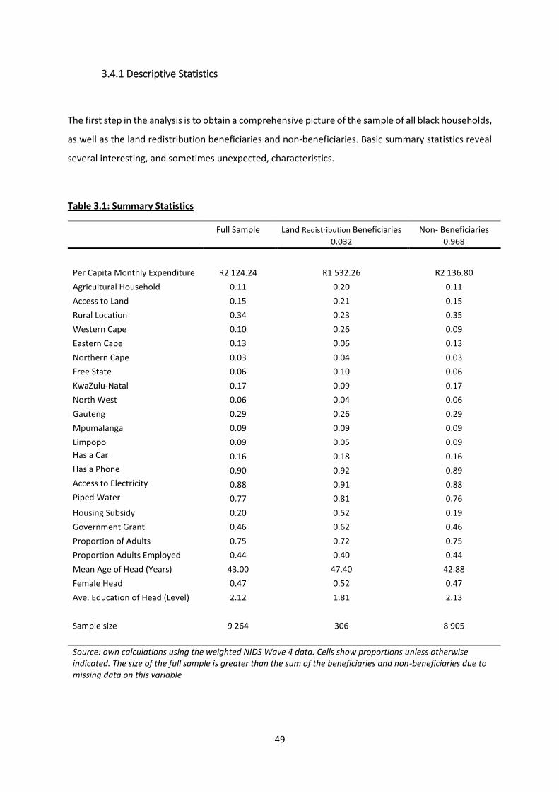
49
3.4.1 Descriptive Statistics
The first step in the analysis is to obtain a comprehensive picture of the sample of all black households,
as well as the land redistribution beneficiaries and non-beneficiaries. Basic summary statistics reveal
several interesting, and sometimes unexpected, characteristics.
Table 3.1: Summary Statistics
Full Sample Land Redistribution Beneficiaries Non- Beneficiaries
0.032 0.968
Per Capita Monthly Expenditure R2 124.24 R1 532.26 R2 136.80
Agricultural Household 0.11 0.20 0.11
Access to Land 0.15 0.21 0.15
Rural Location 0.34 0.23 0.35
Western Cape 0.10 0.26 0.09
Eastern Cape 0.13 0.06 0.13
Northern Cape 0.03 0.04 0.03
Free State 0.06 0.10 0.06
KwaZulu-Natal 0.17 0.09 0.17
North West 0.06 0.04 0.06
Gauteng 0.29 0.26 0.29
Mpumalanga 0.09 0.09 0.09
Limpopo 0.09 0.05 0.09
Has a Car 0.16 0.18 0.16
Has a Phone 0.90 0.92 0.89
Access to Electricity 0.88 0.91 0.88
Piped Water 0.77 0.81 0.76
Housing Subsidy 0.20 0.52 0.19
Government Grant 0.46 0.62 0.46
Proportion of Adults 0.75 0.72 0.75
Proportion Adults Employed 0.44 0.40 0.44
Mean Age of Head (Years) 43.00 47.40 42.88
Female Head 0.47 0.52 0.47
Ave. Education of Head (Level) 2.12 1.81 2.13
Sample size 9 264 306 8 905
Source: own calculations using the weighted NIDS Wave 4 data. Cells show proportions unless otherwise indicated. The size of the full sample is greater than the sum of the beneficiaries and non-beneficiaries due to missing data on this variable

50
Table 3.1 provides summary details for the full black sample, as well as for land redistribution
beneficiary and non-beneficiary households separately. Land redistribution beneficiary households
have considerably lower per capita monthly expenditure than non-beneficiaries, at R1 532.26 and
R2 136.80 respectively. It may appear from this simple statistic that beneficiaries are worse off than
non-beneficiaries in terms of expenditure, however it cannot be ruled out that the expenditure of
beneficiary households has indeed improved from some lower base as a result of receiving a land
redistribution grant. While the greater proportion of beneficiary households having access to land for
farming purposes is encouraging, 0.21 compared to 0.15 of non-beneficiaries, this is still an
unexpectedly low share. This is reflected in the low proportion of beneficiary households involved in
agricultural activity, 0.20, and 0.11 for non-beneficiaries. The low levels of access to land and
agricultural activity of beneficiary households reflect the low correlations observed previously, and
are not what might be expected considering that the purpose of land redistribution is to supply
households with access to land. This raises the important question of what has happened to the land
received through the land redistribution programme, which will be considered later.
The majority of land redistribution beneficiary households are located in urban areas, 0.77, as are the
majority of the sample, 0.66. The urban location of beneficiaries might explain, or at least reflect, to
some extent the lack of access to land and low levels of household agricultural activity observed. A
relatively large proportion of land redistribution beneficiaries are located in the Western Cape, 0.26,
while there are relatively smaller proportions located in the Eastern Cape, 0.06, and KwaZulu-Natal,
0.09.
There is little difference in asset ownership and access to services, while a greater proportion of
beneficiary households receive a housing subsidy and a government grant, 0.52 and 0.62, than non-
beneficiaries, 0.19 and 0.46. This is in keeping with the means tests for these social welfare policies
with only poor households being eligible. Beneficiary and non-beneficiary households are similar in
terms of the composition of the household with respect to the proportion of adults in the household
and the proportion of adults employed in the households. The characteristics of the household head
do not reveal anything of special interest between beneficiaries and non-beneficiaries, with a
somewhat greater proportion of beneficiary heads being female, slightly older, and having slightly
lower levels of education on average.
From the descriptive statistics, it appears that many land redistribution beneficiary households are
not involved in any farming activity, have no access to land, reside in urban areas, and have a lower
per capita expenditure than non-beneficiary households. Based on the purposes and aims of land
redistribution, this depiction is contrary to what one might expect, and requires further consideration.

51
While puzzling, it is worth noting that this characterisation is the same as that observed from a survey
specific to land reform conducted by the Human Sciences Research Council in 2005 (Aliber, Reitzes
and Roefs, 2005). This is discussed further in section 3.5.1. Unfortunately, there is no information in
the data regarding the urban or rural location of the land received through land redistribution, or
about whether respondents are currently residing on the land received. It is thus not clear from the
data if the urban respondents received land located in these urban areas, or if the land is in rural areas
and they do not reside on this land, or if indeed they still own the land.
The indications are however that redistributed land is in the rural areas, and the most likely scenario
is that beneficiaries do not reside on the land received. As discussed in the first chapter outlining the
policy milieu, land redistribution programmes have a strong emphasis on rural development and
increasing rural welfare. As noted in the Reconstruction and Development Programme a land reform
programme “must aim to supply residential and productive land to the poorest section of the rural
population and aspirant farmers … it must raise rural incomes and productivity, and must encourage
the use of land for agricultural and productive or residential purposes” (ANC, 1994, pp 24). While land
in urban areas is not explicitly precluded, it is scarcely mentioned and the emphasis is clearly on rural
land being redistributed. It does not seem likely then that such a great proportion of redistributed
land is located in urban areas. The more plausible scenario is that many of these beneficiaries have
moved from rural to urban areas, and are thus not residing where the redistributed land was or is
located.
Most studies report that redistributed land tends to be underutilised by beneficiaries, for various
reasons (Hall, 2009). Subdivision of large farms acquired for land reform is legal, however very little
formal subdivision has taken place in practice. The structure of the land reform grants and a
bureaucratic insistence on maintaining the original boundaries of transferred farms necessitates the
pooling of resources, with farm purchases by individuals or families being rare. The result is a “curious”
form of collective farming of a single large farm by groups of beneficiaries (Cousins, 2013, pp 13).
Conflicts on these collective farming projects over how land should be used have contributed to the
collapse of many projects, with few beneficiaries successfully farming collectively (Hall, 2009; ARI,
2013). Evidence from case studies supports this indication, suggesting that beneficiaries may not
actually reside on the land received. This is particularly so when the land is owned by a number of
households, as is often the case (Bradstock, 2005). The indication is that the land is often located some
distance from where the beneficiaries live, and the cost of transport prohibits them from regularly
accessing the land and making productive use of it. As a result, a large proportion of land beneficiary
group members are not actively involved in the agricultural projects on their collectively owned land
(Bradstock, 2005). These indications are further underpinned by claims made by the Minister of Rural
52
Development and Land Reform that 90% of land reform projects have failed (Lund, 2012, as cited in
O’Laughlin, Bernstein, Cousins and Peters, 2013)24. Although this is likely an exaggeration with no
empirical evidence to support the claim, it is a clear indication that success rates are low.
While there might be a level of supposition regarding the location of land received, what is less
contentious is the low access to land reported by beneficiaries. Regardless of whether the land
received is in an urban or rural location, the lack of access to land is a strong indication that the land
received may not be used as intended. The low levels of agricultural activity and access to land make
sense considering the urban location of the majority of beneficiaries, and the notion that they are not
residing on the land received.
3.4.2 Further Descriptive Analysis
The NIDS data includes several detailed questions related to the farming activities of the household.
While not explicitly included in the regression analysis, these variables provide useful information and
details about various aspects of household agriculture. This additional information provides a useful
context within which to locate the findings from the analysis.
Table 3.2: Further Summary Statistics
Full Sample Land Redistribution Beneficiaries Non- Beneficiaries
Income from Agriculture R268.43 R924.46 R226.09
Commercial Farming 0.19 0.28 0.17
Livestock 0.46 0.10 0.46
Poultry 0.22 0.02 0.25
Crops 0.68 0.98 0.70
Privately Owned Land* 0.74 0.88 0.73
Land Size* 1.35 1.42 1.30
Farming Inputs 0.96 1.12 0.95
Farming Assets 0.26 0.40 0.26
Source: own calculations using the weighted NIDS Wave 4 data. Cells show proportions unless otherwise stated. * Indicates questions that were only asked of households that report having access to land.
24 The original article by Lund, 2012, in the Financial Mail was not found online.
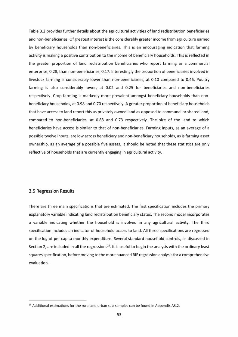
53
Table 3.2 provides further details about the agricultural activities of land redistribution beneficiaries
and non-beneficiaries. Of greatest interest is the considerably greater income from agriculture earned
by beneficiary households than non-beneficiaries. This is an encouraging indication that farming
activity is making a positive contribution to the income of beneficiary households. This is reflected in
the greater proportion of land redistribution beneficiaries who report farming as a commercial
enterprise, 0.28, than non-beneficiaries, 0.17. Interestingly the proportion of beneficiaries involved in
livestock farming is considerably lower than non-beneficiaries, at 0.10 compared to 0.46. Poultry
farming is also considerably lower, at 0.02 and 0.25 for beneficiaries and non-beneficiaries
respectively. Crop farming is markedly more prevalent amongst beneficiary households than non-
beneficiary households, at 0.98 and 0.70 respectively. A greater proportion of beneficiary households
that have access to land report this as privately owned land as opposed to communal or shared land,
compared to non-beneficiaries, at 0.88 and 0.73 respectively. The size of the land to which
beneficiaries have access is similar to that of non-beneficiaries. Farming inputs, as an average of a
possible twelve inputs, are low across beneficiary and non-beneficiary households, as is farming asset
ownership, as an average of a possible five assets. It should be noted that these statistics are only
reflective of households that are currently engaging in agricultural activity.
3.5 Regression Results
There are three main specifications that are estimated. The first specification includes the primary
explanatory variable indicating land redistribution beneficiary status. The second model incorporates
a variable indicating whether the household is involved in any agricultural activity. The third
specification includes an indicator of household access to land. All three specifications are regressed
on the log of per capita monthly expenditure. Several standard household controls, as discussed in
Section 2, are included in all the regressions25. It is useful to begin the analysis with the ordinary least
squares specification, before moving to the more nuanced RIF regression analysis for a comprehensive
evaluation.
25 Additional estimations for the rural and urban sub-samples can be found in Appendix A3.2.
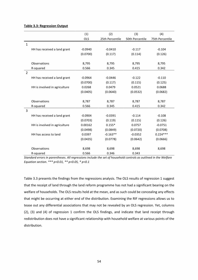
54
Table 3.3: Regression Output
(1) (2) (3) (4)
OLS 25th Percentile 50th Percentile 75th Percentile
1
HH has received a land grant -0.0940 -0.0410 -0.117 -0.104
(0.0700) (0.117) (0.114) (0.126)
Observations 8,795 8,795 8,795 8,795
R-squared 0.566 0.345 0.415 0.342
2
HH has received a land grant -0.0964 -0.0446 -0.122 -0.110
(0.0700) (0.117) (0.115) (0.125)
HH is involved in agriculture 0.0268 0.0479 0.0521 0.0688
(0.0405) (0.0640) (0.0532) (0.0682)
Observations 8,787 8,787 8,787 8,787
R-squared 0.566 0.345 0.415 0.342
3
HH has received a land grant -0.0904 -0.0391 -0.114 -0.108
(0.0703) (0.119) (0.115) (0.126)
HH is involved in agriculture 0.00162 0.155* 0.0757 -0.0751
(0.0498) (0.0849) (0.0720) (0.0708)
HH has access to land 0.0397 -0.163** -0.0352 0.224***
(0.0435) (0.0778) (0.0642) (0.0666)
Observations 8,698 8,698 8,698 8,698
R-squared 0.566 0.346 0.343
Standard errors in parentheses. All regressions include the set of household controls as outlined in the Welfare
Equation section. *** p<0.01, ** p<0.05, * p<0.1
Table 3.3 presents the findings from the regressions analysis. The OLS results of regression 1 suggest
that the receipt of land through the land reform programme has not had a significant bearing on the
welfare of households. The OLS results hold at the mean, and as such could be concealing any effects
that might be occurring at either end of the distribution. Examining the RIF regressions allows us to
tease out any differential associations that may not be revealed by an OLS regression. Yet, columns
(2), (3) and (4) of regression 1 confirm the OLS findings, and indicate that land receipt through
redistribution does not have a significant relationship with household welfare at various points of the
distribution.
55
Regression 2 introduces household agricultural activity to the estimation. Again, neither the OLS nor
the quantile regressions indicate any significant association between land receipt and household
welfare, or between household agricultural activity and welfare. Regression (3) incorporates access to
land into the estimation. Land receipt remains insignificant, as does agricultural activity for the most
part. Controlling for access to land does however result in agricultural activity being positively
significant at the lower end of the distribution, intimating that poorer households can benefit from
farming activity. Access to land itself however has a negative bearing on household welfare at the 25th
percentile, but a significantly positive influence at the 75th percentile. This seems to suggest that only
wealthier households can reap welfare benefits from access to land for farming activities.
The primary observation is that having received a land grant does not appear to have a significant
association with household welfare, across all three of the specifications. This finding holds at the
mean in the OLS regressions, as well as at each quantile of the RIF regressions. These results reflect to
some extent the early indications from the descriptive statistics of the largely unanticipated
characterisation of land beneficiary households. The indication that land receipt does not appear to
have a significant relationship with household welfare supports the arguments questioning land
redistribution as an effective tool for rural economic development and poverty alleviation. Some
possible reasons why the receipt of land may be having a limited impact are suggested by the key
variables in the regression and the descriptive statistics. Most notably the low levels of access to land,
the low proportion of beneficiary households involved in agriculture, and the largely urban location
support the notion of de-agrarianisation in South Africa, and a shift away from rural and agrarian-
based livelihoods in favour of urban living. A key question raised is what has happened to the land
that was received through the programme. A discussion of this question would be purely speculative
at this point as there is unfortunately no data to provide any evidence.
The findings presented here are consistent with the assertion that land-based livelihood strategies, or
subsistence agriculture, may fail to provide a basis for survival (De Swardt, 2003). This is not a
particularly novel perspective, as discussed in the introduction there are numerous doubts about the
capabilities of land redistribution policy to improve the welfare of households. The low levels of
agricultural activity, as well as the largely urban location of beneficiary households observed in the
data, supports the contention that small farmers, rather than landless people, should be targeted for
redistributive land reform policies (Assunção, 2008). The argument is that small farmers are more
likely to have better farming skills and be less willing to sell the land received for consumption
purposes. This policy-targeting suggestion is in accord with the common perception that land
redistribution beneficiaries have not been adequately supported or equipped to initiate even small-
56
scale farming operations. The initial minimum income eligibility criteria of the policy necessarily
implies that beneficiaries may not have the resources or the skills required (Zimmerman, 2000;
Weideman, 2006).
3.5.1 Replication using different data
It is interesting and important to note that the key results found using the nationally representative
NIDS data are reflective of those found doing a similar analysis using a different data set that explores
land reform issues. As part of a larger international project, the Human Sciences Research Council
(HSRC) conducted a survey to assess the alignment of South Africa’s land reform policy to peoples’
aspirations and expectations26. The survey probes issues regarding political participation, preferences
regarding land reform policy, current and past land access and use, land demand, knowledge of land
reform, and overall performance of land reform. Using this data in a UQR analysis of largely similar
welfare equations, the receipt of land and household involvement in agriculture are again found to
not have a persistently significant relationship with household welfare.27
NIDS proved to be the preferred data set for this analysis, with the HSRC data providing a useful check
and balance for the findings. While the data from the HSRC included interesting and unique
information on land reform, the NIDS data is considered more reliable. The HSRC data obtained was
not properly curated, with some doubt over the weighting measures provided. Furthermore, the HSRC
project was only conducted in three provinces, the Free State, the Eastern Cape, and Limpopo, and is
not nationally representative.
3.6 Robustness Tests
A number of methodological and measurement decisions have been made in the analysis, and it is
important to investigate to what extent the results are dependent on these choices. The calculation
of the RIFs involved the selection of bandwidth and the quantiles, both of which are tested here. The
sensitivity of the findings to the choice of the measure of welfare is also tested using two alternative
26 The “Measuring Democracy, Human Rights and Governance” (METAGORA) initiative 27 Author’s own calculations
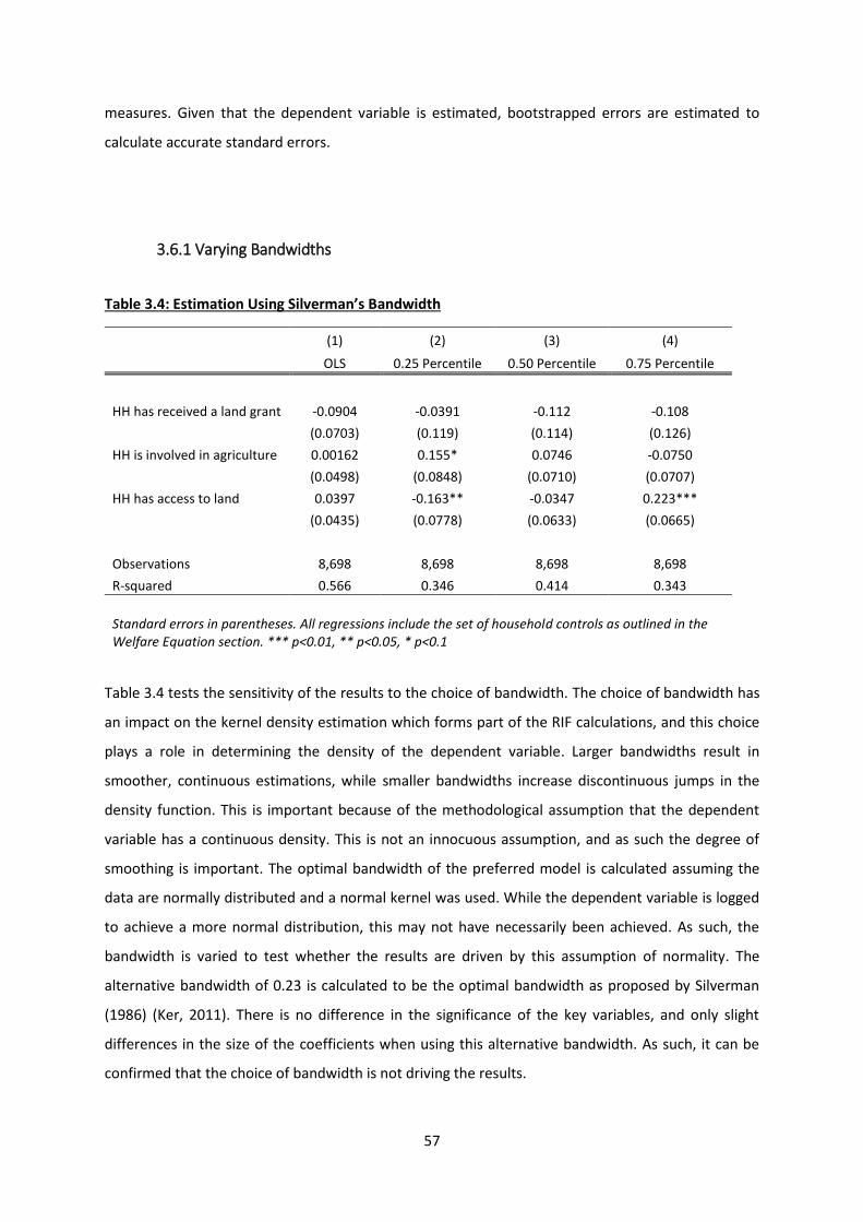
57
measures. Given that the dependent variable is estimated, bootstrapped errors are estimated to
calculate accurate standard errors.
3.6.1 Varying Bandwidths
Table 3.4: Estimation Using Silverman’s Bandwidth
(1) (2) (3) (4)
OLS 0.25 Percentile 0.50 Percentile 0.75 Percentile
HH has received a land grant -0.0904 -0.0391 -0.112 -0.108
(0.0703) (0.119) (0.114) (0.126)
HH is involved in agriculture 0.00162 0.155* 0.0746 -0.0750
(0.0498) (0.0848) (0.0710) (0.0707)
HH has access to land 0.0397 -0.163** -0.0347 0.223***
(0.0435) (0.0778) (0.0633) (0.0665)
Observations 8,698 8,698 8,698 8,698
R-squared 0.566 0.346 0.414 0.343
Standard errors in parentheses. All regressions include the set of household controls as outlined in the Welfare Equation section. *** p<0.01, ** p<0.05, * p<0.1
Table 3.4 tests the sensitivity of the results to the choice of bandwidth. The choice of bandwidth has
an impact on the kernel density estimation which forms part of the RIF calculations, and this choice
plays a role in determining the density of the dependent variable. Larger bandwidths result in
smoother, continuous estimations, while smaller bandwidths increase discontinuous jumps in the
density function. This is important because of the methodological assumption that the dependent
variable has a continuous density. This is not an innocuous assumption, and as such the degree of
smoothing is important. The optimal bandwidth of the preferred model is calculated assuming the
data are normally distributed and a normal kernel was used. While the dependent variable is logged
to achieve a more normal distribution, this may not have necessarily been achieved. As such, the
bandwidth is varied to test whether the results are driven by this assumption of normality. The
alternative bandwidth of 0.23 is calculated to be the optimal bandwidth as proposed by Silverman
(1986) (Ker, 2011). There is no difference in the significance of the key variables, and only slight
differences in the size of the coefficients when using this alternative bandwidth. As such, it can be
confirmed that the choice of bandwidth is not driving the results.
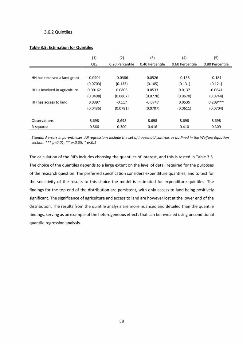
58
3.6.2 Quintiles
Table 3.5: Estimation for Quintiles
(1) (2) (3) (4) (5)
OLS 0.20 Percentile 0.40 Percentile 0.60 Percentile 0.80 Percentile
HH has received a land grant -0.0904 -0.0386 0.0526 -0.158 -0.181
(0.0703) (0.133) (0.105) (0.131) (0.121)
HH is involved in agriculture 0.00162 0.0806 0.0533 0.0137 -0.0641
(0.0498) (0.0867) (0.0778) (0.0670) (0.0744)
HH has access to land 0.0397 -0.117 -0.0747 0.0535 0.209***
(0.0435) (0.0781) (0.0707) (0.0611) (0.0704)
Observations 8,698 8,698 8,698 8,698 8,698
R-squared 0.566 0.300 0.416 0.410 0.309
Standard errors in parentheses. All regressions include the set of household controls as outlined in the Welfare Equation section. *** p<0.01, ** p<0.05, * p<0.1
The calculation of the RIFs includes choosing the quantiles of interest, and this is tested in Table 3.5.
The choice of the quantiles depends to a large extent on the level of detail required for the purposes
of the research question. The preferred specification considers expenditure quantiles, and to test for
the sensitivity of the results to this choice the model is estimated for expenditure quintiles. The
findings for the top end of the distribution are persistent, with only access to land being positively
significant. The significance of agriculture and access to land are however lost at the lower end of the
distribution. The results from the quintile analysis are more nuanced and detailed than the quantile
findings, serving as an example of the heterogeneous effects that can be revealed using unconditional
quantile regression analysis.
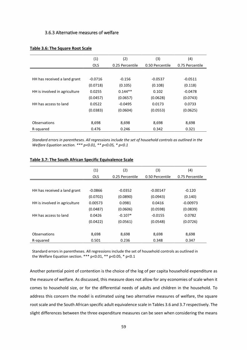
59
3.6.3 Alternative measures of welfare
Table 3.6: The Square Root Scale
(1) (2) (3) (4)
OLS 0.25 Percentile 0.50 Percentile 0.75 Percentile
HH has received a land grant -0.0716 -0.156 -0.0537 -0.0511
(0.0718) (0.105) (0.108) (0.118)
HH is involved in agriculture 0.0255 0.144** 0.102 -0.0478
(0.0457) (0.0657) (0.0628) (0.0743)
HH has access to land 0.0522 -0.0495 0.0173 0.0733
(0.0383) (0.0604) (0.0553) (0.0625)
Observations 8,698 8,698 8,698 8,698
R-squared 0.476 0.246 0.342 0.321
Standard errors in parentheses. All regressions include the set of household controls as outlined in the Welfare Equation section. *** p<0.01, ** p<0.05, * p<0.1
Table 3.7: The South African Specific Equivalence Scale
(1) (2) (3) (4)
OLS 0.25 Percentile 0.50 Percentile 0.75 Percentile
HH has received a land grant -0.0866 -0.0352 -0.00147 -0.120
(0.0702) (0.0890) (0.0943) (0.140)
HH is involved in agriculture 0.00573 0.0981 0.0416 -0.00973
(0.0487) (0.0606) (0.0598) (0.0839)
HH has access to land 0.0426 -0.107* -0.0155 0.0782
(0.0422) (0.0561) (0.0548) (0.0726)
Observations 8,698 8,698 8,698 8,698
R-squared 0.501 0.236 0.348 0.347
Standard errors in parentheses. All regressions include the set of household controls as outlined in the Welfare Equation section. *** p<0.01, ** p<0.05, * p<0.1
Another potential point of contention is the choice of the log of per capita household expenditure as
the measure of welfare. As discussed, this measure does not allow for any economies of scale when it
comes to household size, or for the differential needs of adults and children in the household. To
address this concern the model is estimated using two alternative measures of welfare, the square
root scale and the South African specific adult equivalence scale in Tables 3.6 and 3.7 respectively. The
slight differences between the three expenditure measures can be seen when considering the means
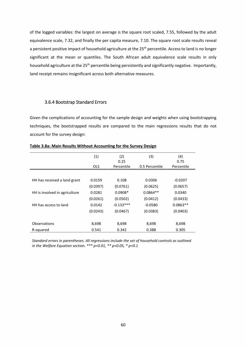
60
of the logged variables: the largest on average is the square root scaled, 7.55, followed by the adult
equivalence scale, 7.32, and finally the per capita measure, 7.10. The square root scale results reveal
a persistent positive impact of household agriculture at the 25th percentile. Access to land is no longer
significant at the mean or quantiles. The South African adult equivalence scale results in only
household agriculture at the 25th percentile being persistently and significantly negative. Importantly,
land receipt remains insignificant across both alternative measures.
3.6.4 Bootstrap Standard Errors
Given the complications of accounting for the sample design and weights when using bootstrapping
techniques, the bootstrapped results are compared to the main regressions results that do not
account for the survey design:
Table 3.8a: Main Results Without Accounting for the Survey Design
(1) (2) (3) (4)
OLS 0.25
Percentile 0.5 Percentile 0.75
Percentile
HH has received a land grant 0.0159 0.108 0.0306 -0.0207
(0.0397) (0.0761) (0.0625) (0.0657)
HH is involved in agriculture 0.0281 0.0908* 0.0864** 0.0340
(0.0261) (0.0502) (0.0412) (0.0433)
HH has access to land 0.0142 -0.133*** -0.0580 0.0863**
(0.0243) (0.0467) (0.0383) (0.0403)
Observations 8,698 8,698 8,698 8,698
R-squared 0.541 0.342 0.388 0.305
Standard errors in parentheses. All regressions include the set of household controls as outlined in the Welfare Equation section. *** p<0.01, ** p<0.05, * p<0.1
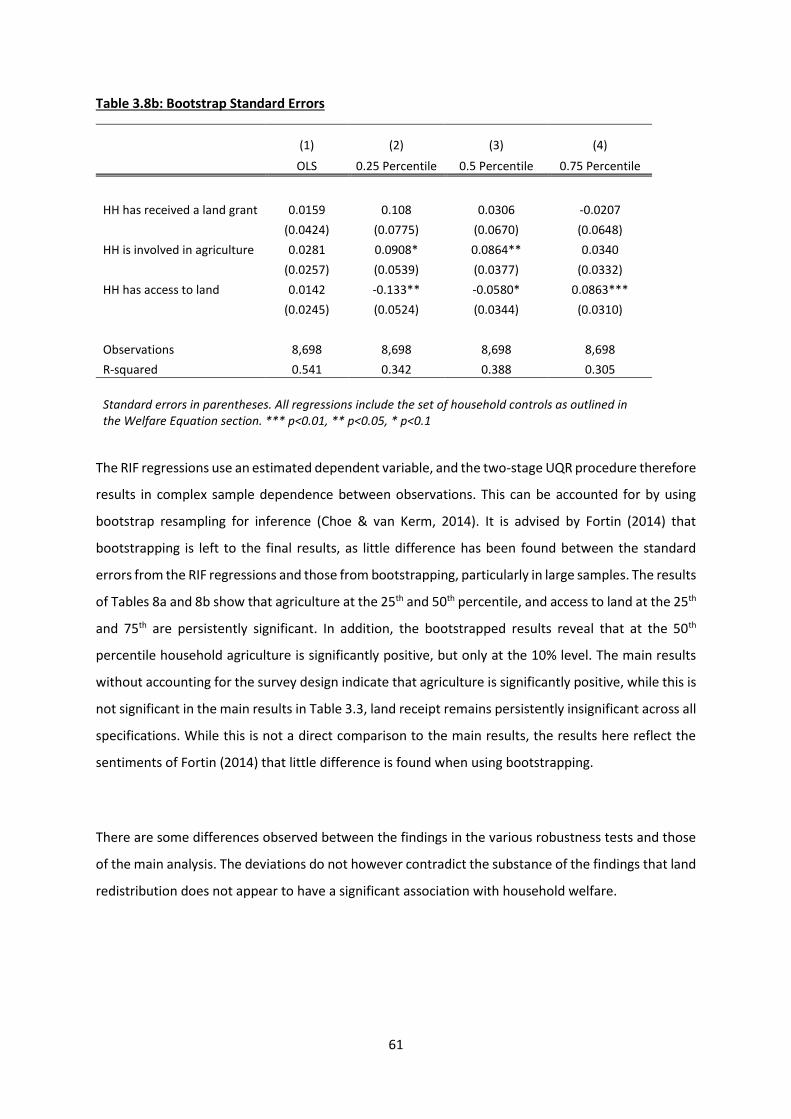
61
Table 3.8b: Bootstrap Standard Errors
(1) (2) (3) (4)
OLS 0.25 Percentile 0.5 Percentile 0.75 Percentile
HH has received a land grant 0.0159 0.108 0.0306 -0.0207
(0.0424) (0.0775) (0.0670) (0.0648)
HH is involved in agriculture 0.0281 0.0908* 0.0864** 0.0340
(0.0257) (0.0539) (0.0377) (0.0332)
HH has access to land 0.0142 -0.133** -0.0580* 0.0863***
(0.0245) (0.0524) (0.0344) (0.0310)
Observations 8,698 8,698 8,698 8,698
R-squared 0.541 0.342 0.388 0.305
Standard errors in parentheses. All regressions include the set of household controls as outlined in the Welfare Equation section. *** p<0.01, ** p<0.05, * p<0.1
The RIF regressions use an estimated dependent variable, and the two-stage UQR procedure therefore
results in complex sample dependence between observations. This can be accounted for by using
bootstrap resampling for inference (Choe & van Kerm, 2014). It is advised by Fortin (2014) that
bootstrapping is left to the final results, as little difference has been found between the standard
errors from the RIF regressions and those from bootstrapping, particularly in large samples. The results
of Tables 8a and 8b show that agriculture at the 25th and 50th percentile, and access to land at the 25th
and 75th are persistently significant. In addition, the bootstrapped results reveal that at the 50th
percentile household agriculture is significantly positive, but only at the 10% level. The main results
without accounting for the survey design indicate that agriculture is significantly positive, while this is
not significant in the main results in Table 3.3, land receipt remains persistently insignificant across all
specifications. While this is not a direct comparison to the main results, the results here reflect the
sentiments of Fortin (2014) that little difference is found when using bootstrapping.
There are some differences observed between the findings in the various robustness tests and those
of the main analysis. The deviations do not however contradict the substance of the findings that land
redistribution does not appear to have a significant association with household welfare.
62
3.7 Conclusion
The efficacy of land redistribution policy remains a contested issue. The debate is largely discursive,
and there is a shortage of empirical evidence either supporting or refuting the arguments for and
against land redistribution. Currently these discussions are largely based on case studies and
theoretical discussion, with a few exceptions such as Keswell & Carter (2010) and Valente (2009).
Using survey data, this research has attempted to explore the function that land redistribution policy
has played in shaping household welfare, as well as the role played by household agriculture and
access to land. To understand the role of land redistribution and household agriculture, a simple
model of household expenditure determination has been estimated, using unconditional quantile
regression analysis to allow for the possibility of heterogeneity in covariate effects.
The analysis considered various aspects and concepts associated with land redistribution policy. First
and foremost, the role played by having received a land grant is estimated. Following this, two
‘transmission mechanisms’ as it were of land redistribution are considered: agricultural activity and
access to land. A strong assumption of land reform policy is that land redistribution will lead to
increased agricultural production because of increased access to land. It is this increased agricultural
production that is presumed to lead to improved household welfare. The findings here however
suggest that the receipt of land does not have a significant association with per capita household
expenditure, either at the mean or at various points in the expenditure distribution. Having
established that land received through land redistribution programmes does not necessarily translate
into increased agricultural activity, the function played by household farming is considered separately,
and it too is found to not have a persistently significant bearing on welfare. Given that land beneficiary
households may not be engaging in agricultural activity, the next question to consider is access to land.
The descriptive statistics indicate that, like agricultural activity, a low proportion of beneficiaries
report access to land. Again, the results suggest that access to land does not have a significant
influence on household welfare. The overall impression from this chapter is that being a beneficiary
of land redistribution may not necessarily lead to welfare improvement, possibly because it does not
seem to lead to increased agricultural activity or access to land. Furthermore, access to land and
agricultural activity themselves do not seem to have a persistently significant association with
household welfare.
Policy making in general is a process informed by assumptions concerning the objectives of the policy
and how these objectives can be achieved. Policy formulation also reflects the distribution of power
within a society with subsequent policy reflecting the roles and influence of these groups in the
process (Weideman, 2004). If the assumptions of policy makers are not informed and/or shared by
63
the stakeholders involved, such as potential beneficiaries of the programmes, the policy runs the risk
of being unsustainable in the long run (Aliber, Reitzes, & Roefs, 2006). The needs and wants of target
groups and beneficiaries play a core role in determining the long-term success and sustainability of a
policy. This is particularly so in the case of land redistribution where the process is largely demand
driven, and where effective participation, and ultimately productive success, requires considerable
effort on the part of applicants and beneficiaries. The characteristics of beneficiary and non-
beneficiary households revealed here are perplexing, and not in keeping with the assumptions
discussed in the policy documentation. An issue that is particularly concerning is the lack of access to
privately-owned land by land redistribution beneficiaries. The analysis suggests that the land is not
being used productively, or indeed accessible by beneficiaries. However, questions about what has
happened to the land received by beneficiaries are not addressed in this survey, or any other. A
thorough examination of this question would be very useful in providing insights into why we might
observe such limited welfare outcomes of land redistribution.
This research is one of only a few studies providing quantitative evidence on the influence of land
redistribution policy on the welfare of beneficiary households in South Africa. Such approaches to
welfare estimation are arguably plagued by econometric issues, and while this does not render the
findings obsolete, there are possible improvements. An experimental design that avoids endogeneity
concerns through randomisation would provide more rigorous evidence. Given that an experimental
study is not always possible, subjective measures of welfare and poverty can also be used to mitigate
endogeneity issues in poverty and welfare research (Ravallion, 2014). While the indications from this
analysis are more suggestive than conclusive, it is worth noting that comparable characterisations and
associations were found when a very similar analysis was conducted using a different data set. As a
first attempt at quantitatively exploring the relationship between land and household welfare
outcomes, the findings presented in this chapter do not offer conclusive evidence of any significant
impact of land redistribution. The lack of result is an interesting descriptive finding in and of itself, and
calls for further analysis. The following two chapters build on this foundation, and utilise a novel
framework for measuring the food insecurity outcomes of land beneficiaries in a more targeted
fashion.
64
Chapter 4: Multidimensional Food Insecurity
Measurement
4.1 Introduction
Chapter 3 of this research considered a generalised model of household welfare in exploring what
influence land redistribution and household agricultural activity might have on welfare. The chapter
proved useful as a first look at the main questions of the research, and while it did suggest that
redistributed land might not be widely effective in improving household welfare, the overall
impression from the results might be considered equivocal. In this next chapter the focus is narrowed
from general household welfare to food insecurity as a specific measure of welfare. Food insecurity
plays a prominent role as a primary goal of land reform policy, and is a natural next step in assessing
the function of land in household prosperity. The first step, as outlined in this chapter, involves the
development of a new multidimensional measure of food insecurity, as existing measures of food
insecurity are largely inadequate for capturing the complex nature of what it means to be food
insecure. This includes a detailed food insecurity profile of South Africa. In the following chapter the
new index is used in assessing the role of land redistribution in influencing household food insecurity.
“Food security exists, at the individual, household, national, regional, and global
levels when all people, at all times, have physical, social and economic access to
sufficient, safe, and nutritious food to meet their dietary needs and food preferences
for a healthy and active life” (FAO, 2001).
The definition of food security cited above enjoys widespread agreement. Yet there is no singular
measure of food security that has been accepted as the ‘gold’ standard when it comes to measuring
household food security. Dissatisfaction with existing food security measures is not new, and multiple
measures are used in the literature, each capturing various aspects of food insecurity (Headey & Ecker,
2013). Internationally there has been a shift in the thinking about food security from a ‘first
generation’ focus on aggregate food availability (supply side), to a ‘second generation’ emphasis on
individual and household food security (demand side), and finally toward a ‘third generation’ that
locates food security in a broader framework of individual behaviour and perceptions (Barrett, 2002).
65
These changes are reflected in the South African context where there have been two major shifts in
the focus on food security: Firstly from the national to the household level; and secondly from the use
of objective measures to subjective perceptions (Hart, 2009).
It is well established that food security is too complex a phenomenon to be captured by a single
indicator and needs to be treated as a multidimensional concept, but that it is very hard to give
recognition to such multidimensionality in measurement. This discussion tracks a very similar
discussion in the literature on measuring poverty.28 There too has been a strong movement for the
adoption of a multidimensional approach to poverty, with a number of authors recognising the variety
of deprivations experienced by those in poverty, and the need for an overarching framework to
incorporate these.29 In an effort to address this gap in food security measurement, the assumption
here is that the complex nature and measurement of food insecurity is analogous to that of poverty,
to the extent that it can be argued that food insecurity is a special case, or manifestation, of poverty.
It is thus a natural extension to apply the method of capturing the multiple dimensions of poverty in
a single index to the measurement of food insecurity.
This paper proposes a new multidimensional index for measuring food insecurity, based on the
method developed by Alkire & Foster (2009; 2011). The Alkire-Foster method is a general framework
for the measurement of poverty as a multidimensional concept. Many of the key decisions are left to
the user, including the variables or dimensions used, the cut-offs, and the weights which can be varied
to fit the purpose of the measure (Alkire & Foster, 2011). The Multidimensional Food Insecurity Index
(MFII) exploits this ‘general framework’ in its construction, using food security specific dimensions,
cut-offs, and weights. One specific measure that has been developed using the framework, the
Multidimensional Poverty Index (MPI), is particularly relevant and is used as the foundation for the
measurement of multidimensional food insecurity. The result is an aggregate measure of food
insecurity that reflects the prevalence of food insecurity, as well as the joint distribution of
deprivation.
In working towards a more comprehensive understanding of what it means to be food insecure, a
multidimensional food insecurity index can lead to better policy-making, as is argued in the poverty
context (Finn, Leibbrandt & Woolard, 2013). The properties of the MFII that enable the identification
of major contributors to household and individual food insecurity, and the ability to examine the depth
and breadth of the problem, allows for the development of more targeted policies to address the most
28 For example Maxwell et al, 1999; Hart, 2009; Coates et al, 2007; Coates et al, 2006; Battersby, 2012. 29 See Sen, 2000; Alkire & Foster, 2009 & 2011; Bourguignon & Chakravarty, 2003; Duclos et al, 2006; Atkinson, 2003.
66
pressing problems. While much of this paper is a contribution to the theory of food insecurity
measurement, particularly in the multidimensional framework, the results are also important for
applied food security analysis. The index is used to develop a detailed food insecurity profile of South
Africa, which highlights the indicators and sub-populations of greatest concern.
In terms of structure, each section of the paper begins with a discussion of the Alkire-Foster method
and some technical details, followed by the application in the food security context. Section 2
introduces the Alkire-Foster framework and the choice of dimensions and indicators. The selected
variables for the MFII are discussed in some detail, as are the within indicator cut-offs. The Alkire-
Foster aggregation procedure, including cross-indicator cut-offs and weights, is then outlined,
followed by the application to the MFII. The decomposition properties of the Alkire-Foster framework
are discussed, before a detailed profile of multidimensional food insecurity in South Africa is
presented. Robustness checks are presented in Section 3, followed by a policy discussion and
conclusion in Section 4.
4.2 Developing the Multidimensional Food Insecurity Index
While South Africa is considered food secure at the national level, many households suffer from
chronic and transitory food insecurity as measured by numerous indicators (Department of
Agriculture, 2003; HSRC, 2004).30 The 1995 Income and Expenditure Survey found an urban food
poverty rate of 27% compared to a rural rate of 54% (Rose & Charlton, 2002). The National Food
Consumption Survey of 1999 found levels of urban food insecurity of 42%, compared to 62% in rural
areas. Using a 24-hour recall period the South African Social Attitudes Survey (SASAS) found that 38.3%
of South Africans have poor food security (Labadarios, Steyn & Nel, 2011). These varying levels of food
insecurity between surveys can be attributed to the survey tools and proxies that have been used to
measure food insecurity.
Aside from the problem of inconsistent measurement of food insecurity across these measures, each
of these tools has weaknesses in assessing the depth or severity of food insecurity. For example,
Valente (2009) makes use of a question concerning the prevalence of hunger in the household as a
measure of food insecurity. However, food insecurity is not synonymous with hunger. Hunger is the
extreme end of food insecurity, and as such this measure may miss out on food insecure households
30 For discussion on household level food security see Hart, 2009; Hendriks, 2005, and Aliber, 2009.
67
that do not fall into hunger (Battersby, 2012). On the other hand, the SASAS study made use of dietary
diversity as a proxy for food insecurity (Labadarios et al, 2011). While this dietary diversity approach
has been widely used and has its strengths, it does not make any reference to the adequacy of the
quantity of food consumed, either objectively or subjectively. Income and expenditure as measures
of food security may also obscure the true extent of food insecurity as prices vary across urban and
rural locations, as well as across provinces. Furthermore, the amount spent, even only on food, gives
no indication of the nutrient quality and diversity of the consumption bundle.
For these reasons, it is widely recognised that studies making use of single measures are likely to miss
the complexity of the experience that characterises food insecure households and individuals. While
the need for a measure that incorporates the multiple experiences of food insecurity is undisputed,
the method of doing so has not been so obvious. One promising avenue is to employ the Alkire-Foster
methodology of multidimensional poverty measurement. The methodology of multidimensional
poverty measurement forms the basis for the development of the multidimensional food insecurity
measure. While this is not a paper about poverty measurement, a discussion of this original
methodology will lay the foundation for the creation of the Multidimensional Food Insecurity Index31.
As such, in each section, a conceptual discussion of the Alkire-Foster and MPI methodology precedes
the application to the development of the MFII.
4.2.1 Dimensions, Indicators, and Cut-offs of the Index
As noted by Alkire & Foster (2011) the aim of the development of the MPI was two-fold in terms of
practical and theoretical goals. From the practical perspective, the purpose was to construct a
measure that could be used with continuous and cardinal data. A theoretical goal was to re-examine
the identification step – who is poor. The outcome is a measure that first identifies who is poor in
each dimension, and then aggregates to obtain group measures that reflect the multiple deprivations
experienced by the poor.
Sen (1976) highlights two distinct problems that must be faced when measuring poverty:
i) Identifying the poor among the total population, and
ii) Constructing an index of poverty using the available information on the poor.
31 For the full details of the multidimensional poverty measures and the MPI see Alkire & Foster 2009 & 2011. The 2011 paper provides useful detail and explanations, once the 2009 paper has been studied carefully.
68
The first problem involves the choice of a criterion of poverty, a cut-off point that determines poverty,
such as a poverty line. The second involves the process of developing an index once the poor have
been identified. As noted by Sen at the time, much had been done to address the first problem, while
little advancement had been made in respect to the second problem (1976). Several authors have
since recognised the need to consider poverty as multidimensional when addressing the second
problem of constructing the index. For example, Bourguignon & Chakravarty (2003) argue that
poverty should be regarded as the failure to reach ‘minimally acceptable’ levels of different monetary
and non-monetary attributes necessary for a subsistence standard of living, highlighting the
multidimensional nature of the phenomenon.
Prior to the multidimensional poverty measurement developed by Alkire & Foster (2009) other
methods aimed at accounting for the multidimensional nature of poverty did incorporate multiple
dimensions. These aggregate indices however add up the dimensions and then apply an aggregate
cut-off to determine who is poor. This has the result of converting the multiple dimensions of poverty
into a unidimensional measure, ensuing in a loss of information on deprivations in specific indicators
(Alkire & Foster, 2009). Conversely, the Alkire-Foster method defines a poverty level within each
indicator before aggregating across dimensions. In this way, the contribution of each indicator to
overall poverty is preserved.
The method proposed makes use of a dual cut-off in identifying the poor. First there is a within
dimension cut-off identifying those who are deprived in each indicator, then there is the across
dimension cut-off identifying those who are deprived in a minimum number of indicators to be
identified as being multidimensionally poor. The cross-dimensional cut-off extends the traditional
union and intersection approaches of identification, resulting in measures that have numerous key
properties for analysis (Alkire & Foster, 2009). The union and the intersection approaches are two
common criteria for identification of the poor, each with their own limitations. In the union approach
a person is said to be multidimensionally poor if they are deprived in at least one indicator. This
however could lead to much of the population being identified as poor even when they are not. This
is especially true if there are many dimensions, some of which could be caused by factors other than
being poor. As such, the union method can result in overstating the problem, and is not always suitable
in the identification of the poor. The intersection approach on the other hand only identifies
individuals as being poor if they are deprived in all indicators. While this method is appropriate in
identifying those in extreme poverty, it will exclude those who are deprived in several indicators, but
not necessarily in every indicator. As such this approach is likely to understate the true extent of
poverty (Alkire & Foster, 2009).
69
The dual cut-off method has numerous desirable properties as outlined by Alkire and Foster (2009).
Firstly, it is ‘poverty focused’ in that an increase in the achievement level of a non-poor person leaves
its value unchanged as only the poor are included in the measure. Secondly, it is ‘deprivation focused’
in that an individual’s poverty status is not affected by changes in the levels of non-deprived
achievements. Thirdly, cardinalisations of ordinal variables yield identical conclusions regarding
whether a person is deprived in that dimension and whether he/she is identified as poor.32 The
implication is that the method can be meaningfully applied to data with lower level measurements
properties, such as ordinal data. This greatly extends the usefulness of the approach.
The three dimensions of the MFII are guided by the ‘domains’ of food security as identified by Coates,
Frongillo, Rogers, Webb, Wilde, & Houser (2006).33 Domains are defined as the most core experiences
of food insecurity that are common across countries and cultures. As identified in a cross-country food
security literature review, they are (Coates et al, 2006):
1. Anxiety and uncertainty about the household food supply
2. Insufficient quality (including variety and preferences of the type of food)
3. Inadequate quantity (including the physical consequences)
Additionally, these domains capture the identifiable ‘elements’ of the FAO definition of food security
stated in the introduction (Maxwell, Coates & Vaitla, 2013).34 The different experiences of food
insecurity captured by these domains are also reflected in Maxwell et al (2013), where indicators of
food insecurity are classified into recognisable categories: Dietary diversity and food frequency,
spending on food, consumption behaviours, experiential measures, and self-assessment measures.
Furthermore, the domains consider both subjective and objective measures of food insecurity, an
important consideration as highlighted by Barrett (2010).
Thus, the three domains outlined by Coates et al (2006) are widely accepted. As such they form a solid
basis for three widely accepted dimensions of food security to be included in the index. As shown in
32 Cardinalisations are found by applying a monotonic transformation to the ordinal variable and its cut-off, transforming it into a cardinal variable. 33 There is a fourth dimension measuring ‘social unacceptability’ in terms of consumption or procurement. This domain is often excluded from studies because these questions are too sensitive to be asked outright and as such there is no data (Coates et al, 2006). This is the case in the NIDS data where such questions have not been asked, and thus this domain is omitted. 34 “Food security exists, at the individual, household, national, regional, and global levels when all people, at all times, have physical, social and economic access to sufficient, safe, and nutritious food to meet their dietary needs and food preferences for a healthy and active life” (FAO, 2001).
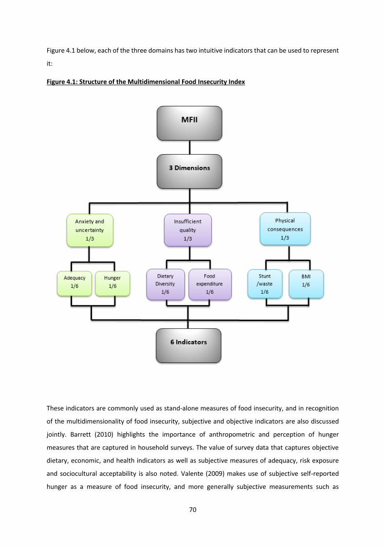
70
Figure 4.1 below, each of the three domains has two intuitive indicators that can be used to represent
it:
Figure 4.1: Structure of the Multidimensional Food Insecurity Index
These indicators are commonly used as stand-alone measures of food insecurity, and in recognition
of the multidimensionality of food insecurity, subjective and objective indicators are also discussed
jointly. Barrett (2010) highlights the importance of anthropometric and perception of hunger
measures that are captured in household surveys. The value of survey data that captures objective
dietary, economic, and health indicators as well as subjective measures of adequacy, risk exposure
and sociocultural acceptability is also noted. Valente (2009) makes use of subjective self-reported
hunger as a measure of food insecurity, and more generally subjective measurements such as
71
perceptions and experiences of hunger broaden the understanding of the multiple factors involved in
food security (Hart, 2009).
Previously, measuring per capita caloric intake or the adequacy of household food availability over
time have been suggested as the main ‘benchmark’ measures for food security at the household level,
and anthropometric measures at the individual level (Maxwell et al, 2013). Undernourishment, as
measured by anthropometric indicators, is also used to measure and distinguish short and long term
food security. Aspects of child malnutrition, such as stunting and wasting, as well as subjective
measures of food insecurity are referred to in a Human Sciences Research Council position paper
measuring food security in South Africa (De Klerk, Drimie, Aliber, Mini, Makoena, Randela, Modiselle,
Roberts, Vogel, de Swardt & Kirsten, 2004).
Together with anthropometrics, dietary diversity and food expenditure are popular objective
measures of food insecurity. The Household Food Insecurity Access Scale (HFIAS) and the Household
Dietary Diversity Score (HDDS) are surveys that capture various objective components of the concept
of food security. The HFIAS measures the access component of food insecurity, while the HDDS
measures dietary diversity in terms of the number of food groups consumed in a day (Coates, Swindale
& Bilinsky, 2007; Swindale & Bilinsky, 2006). In estimating the prevalence of food insecurity in South
Africa, Rose & Charlton (2001 & 2002) employ a quantitative objective measure termed ‘food poverty’
which assesses whether the amount spent by a household on food was adequate to purchase a low-
cost food plan. The MFII manages to incorporate these diverse objective and subjective measures.
4.2.2 Data
The MFII is constructed using the National Income Dynamics Study (NIDS) data presented in Chapter
3. The first wave of this intensive effort to track and follow the life changes of about 28 000 people
was conducted by the Southern African Labour and Development Research Unit SALDRU (Leibbrandt
et al, 2009). While the second and third waves of the panel are publicly available, the approach in this
paper is cross-sectional, with the data coming from the first wave which was conducted in 2008. Later
waves of the data are unfortunately not suitable for this analysis as they do not contain some of the
key variables used in the construction of the index. Wave 1 includes information on households as
well as individuals in the household, and both levels of information are used in this chapter. Version
5.2 of the Wave 1 data includes provincial and geographic type (urban or rural) data based on the
2011 census. These 2011 variables are used in the analysis as they are closer to the survey year. Certain
72
groups were underrepresented in the sample and thus it is appropriate to use post stratification
weights in the analysis to provide a nationally representative analysis (Southern Africa Labour and
Development Research Unit, 2014).
4.2.3 The Indicators
The general methodological framework of the adjusted headcount ratio can be applied to any
dimensions, with the choice being guided by the question of interest. As discussed, the dimensions,
or domains, adopted for the MFII are those defined by Coates et al (2006). The indicators of which the
domains are comprised are those that measure and capture the concepts covered by the domain: BMI
and child stunting and wasting are measures of the physical consequences of food insecurity; self-
reported hunger and perceptions of food adequacy are measures of anxiety and uncertainty about
food supply; and dietary diversity and the proportion of food expenditure capture the quality of the
food consumed. These measures themselves are common indicators of food insecurity, and the cut-
offs within each indicator are guided by the literature.
Dietary Diversity
Dietary diversity, or the number of unique foods consumed over a given period, is considered a
promising measure or indicator of food insecurity, and has previously been considered the “best
performing” (Hoddinott & Yohannes, 2002; Swindale & Bilinsky, 2006). To define unique foods, the
Household Dietary Diversity Score indicator guide identifies twelve food groups, derived from the
United Nations Food and Agriculture Organisation’s Food Composition Table for Use in Africa
(Swindale & Bilinsky, 2006).35 Knowing, for example, that a household consumed an average of four
different food groups in the past 30 days implies some diversity in the macro and micro-nutrients
being consumed. Consumption of different food items is less meaningful in that all four items might
be from the same food group, for example cereals (Swindale & Bilinsky, 2006). Following this
reasoning, the food items listed in the NIDS data were grouped into twelve food groups, based on the
FAO table:
1. Cereals and Grain Products
2. Starchy Roots, Tubers, and Fruits
35 This set of food groups is derived from the U.N. Food and Agriculture Organization (Food and Agricultural
Organization. Food Composition Table for Africa. Rome, Italy, 1970. As viewed at www.fao.org/docrep/003/X6877E/X6877E00.htm.
73
3. Grain Legumes and Legume products
4. Vegetables and Vegetable Products
5. Fruits and Nuts
6. Sugars and Syrups
7. Meats, Poultry, and Insects
8. Eggs
9. Fish and Shellfish
10. Milk and Milk Products
11. Oils and Fats
12. Miscellaneous (including beverages)
The recall period of the food consumption variables in NIDS is the previous 30 days. This lengthy recall
period can result in less accurate information due to imperfect recall, however it can also increase the
confidence with which a household can be classified as food insecure (Swindale & Bilinsky, 2006). The
longer measurement period allows for greater diversity in consumption as opposed to consumption
over, say, a 24-hour period.36 The likelihood of committing a Type II error and classifying households
as food insecure when they are not, based on diversity, is thus reduced.
An increase in the average number of different food groups consumed provides a quantifiable
measure of improved household food access. There is however no explicit number of different food
groups that serves as a cut-off point in differentiating food secure from food insecure households.
One suggestion in the HDDS guide is to take the average diversity of the upper tercile of household
diversity scores (Swindale & Bilinsky, 2006). An alternative measure, which in a sense can be
considered as a less strict measure resulting in a greater count of deprivation, would be to use the
average dietary diversity as a cut-off point, with households who score below average identified as
food insecure. The advantage of both methods is that the target has been shown to be achievable by
the sample population (Swindale & Bilinsky, 2006). This does however result in the measure being a
relative one rather than an absolute one (Maxwell, Ahiadeke, Levin, Armar-Klemesu, Zakariah &
Lamptey, 1999). In the first instance the second option of using the average diversity as the cut-off
has been chosen, largely as a consequence of the average dietary diversity score being high at more
than 9 out of a possible 12. As mentioned this high average could in part be due to the 30-day recall
period.
36 24 hours is the suggested recall period in the HDDS manual (Swindale & Bilinsky, 2006), while the HFIAS utilises a 4-week recall period (Coates, Swindale and Bilinsky, 2007)
74
In the NIDS data 12 households report positive expenditure on food items, while not having consumed
any of the 12 food groups. On further inspection 9 of these households reported consumption of food
hampers, but the contents of these hampers are not known. 3 of the households that report positive
food expenditure report no consumption of any of the food items listed. All 12 of these households
are excluded from the sample as the required information is missing.
Food expenditure
Food expenditure has been used fairly extensively as an indicator of food insecurity, with the general
classification being that households that spend a high proportion of their total expenditure on food
are more vulnerable to food insecurity than those that spend a lower proportion (Maxwell et al, 1999;
Jonnson & Toole, 1991). The rationale is that households that spend a large proportion on food are
more susceptible to changes in food prices, as well as changes in income, than households who spend
a small proportion. Of the income and expenditure measures, food expenditure per capita has been
shown to more accurately identify food insecure households than total expenditure per capita, or
household income (Haddad, Kennedy & Sullivan, 1994).
While commonly used as a proxy for food security, food expenditure may not speak to consumption
differences. This would depend on what kind of food is available in the market and at what prices. For
example, a household that does not receive a regular income, so cannot plan spending, and does not
have storage capacity or access to a supermarket, may spend considerably more on less diverse and
nutritious food than a household with regular income, storage capacity, and access to a supermarket.
Furthermore, this indicator may not capture food that is received as gifts or produced by the
household (Battersby, 2012).
Nevertheless, food expenditure is a useful factor in an index. The variable constructed using the data
captures the total food expenditure of the household in the last 30 days, and is taken as a proportion
of total household expenditure over the same period. As suggested by Maxwell et al (1999) a high
food expenditure proportion is regarded as 60% and above, and these households are classified as
food insecure.37 The index utilises the inverse of this, the proportion of non-food expenditure, as the
indicator. This is for ease of interpretation in that a decrease in the indicator equates to greater
deprivation in terms the proportion of income spent on food.
37 An alternative uses the mean food share figure for the lowest expenditure quintile as the cut-off (Maxwell et al, 1999).
75
Anthropometrics
There are a number of anthropometric measures used as an indication of an adequately nutritious
diet. These measures vary between young children, older children and adolescents, and adults.
Commonly used measures for young children between the ages of 0 and 5 are z-scores for height for
age, and weight for height. These compare the measurements for the child to standard measurements
of a reference population of children. A child is classified as undernourished if his/her z-score is more
than two standard deviations below the median z-score. Stunting is reflected by low height-for-age,
and is associated with several long-term factors such as chronic insufficient protein and energy intake,
sustained poor feeding practices, frequent infections, and certain micronutrient deficiencies.38
Stunting does not change rapidly, and it may be irreversible in children older than two years (Cogill,
2003). Wasting is reflected by low weight-for-height, and is a short-term measure of malnutrition as
wasting can change rapidly with changes in diet and disease prevalence. Causes include inadequate
food intake, poor feeding practices, disease, and infection, or mostly a combination of these (Cogill,
2003). Z-scores are a strong indicator of long and short term food insecurity. Stunting is used as an
indicator for chronic malnutrition and is a bigger problem in South Africa than acute malnutrition, as
measured by wasting (Faber & Wenhold, 2007). At the national level, stunting affects almost one out
of five children (Labadarios, Swart, Maunder, Kruger, Gericke, Kuzwayo, Ntsie, Steyn, Schloss,
Dhansay, Jooste, Dannhauser, Nel, Molete & Kotze, 2008). As part of the NIDS Wave 1 questionnaire
weight and height measurements were taken for all children, and these were used to generate weight-
for-height and height-for-age z-scores for children aged 0 to 5. Children are classified as
undernourished if their stunting or wasting z-score is more than two standard deviations below the
reference group using the WHO international child growth standards (WHO, 2006).
For older children between the ages of 6 and 19 BMI-for-age scores are used as an indicator of
adequate nutrition. The BMI of adults remains relatively constant unless there is weight gain or loss,
and as such it is possible to use the same thresholds for the classification of individuals as underweight,
overweight, or obese regardless of the age and sex of the adult. The BMI of children however changes
as they mature, and these patterns differ between boys and girls (Dinsdale, Ridler & Ells, 2011).
Stratification by age and gender is thus required for this age group to correctly classify individuals
based on their BMI (de Onis, Onyango, Borghi, Siyam, Nishida & Siekmann, 2007). BMI is calculated as
height divided by weight squared, which is then compared to a reference population of children of the
same age and gender.39 Children who have a BMI less than two standard deviations below the median
BMI for the reference group are classified as underweight (Dinsdale et al, 2011). The classification of
38 Particularly iron and zinc 39 Using the 2007 WHO reference charts for boys and girls available at http://www.who.int/growthref/en/
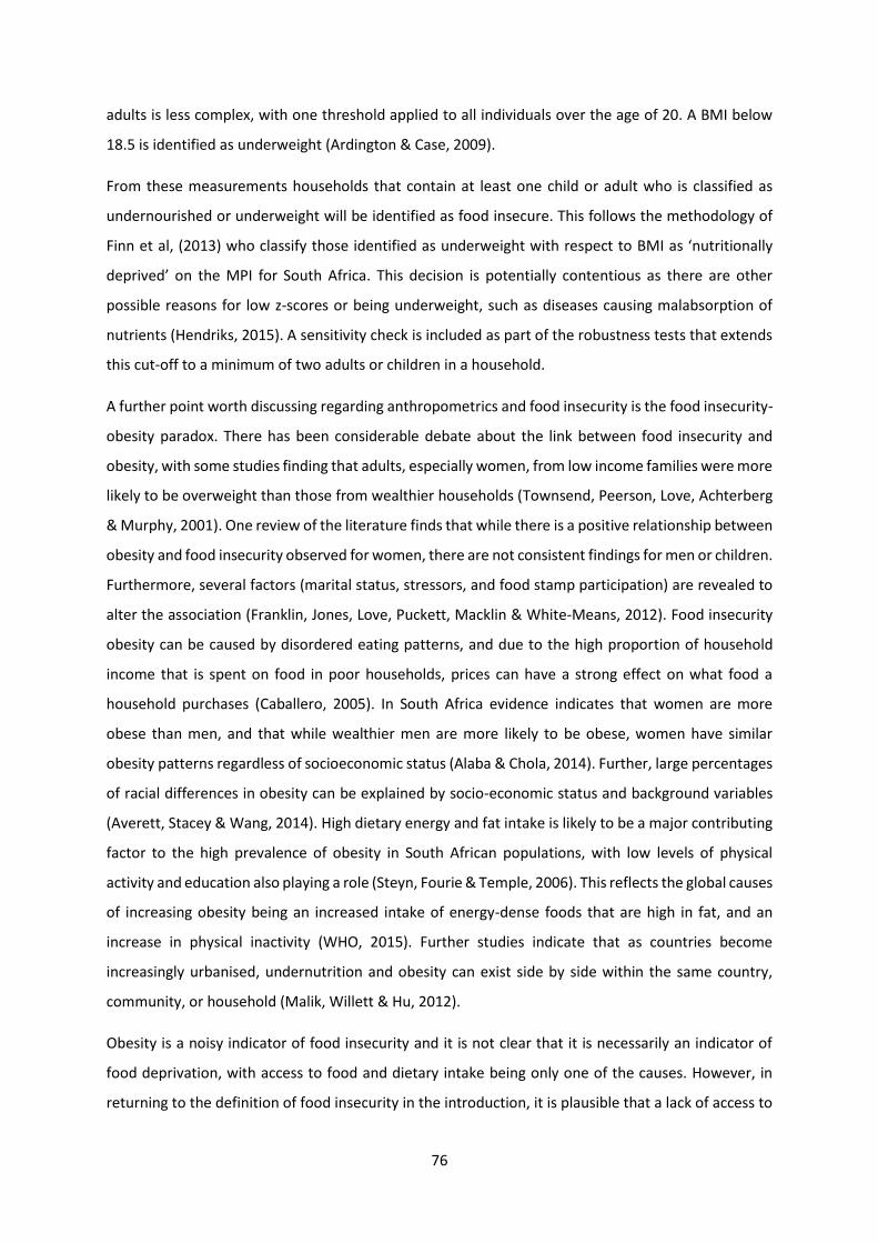
76
adults is less complex, with one threshold applied to all individuals over the age of 20. A BMI below
18.5 is identified as underweight (Ardington & Case, 2009).
From these measurements households that contain at least one child or adult who is classified as
undernourished or underweight will be identified as food insecure. This follows the methodology of
Finn et al, (2013) who classify those identified as underweight with respect to BMI as ‘nutritionally
deprived’ on the MPI for South Africa. This decision is potentially contentious as there are other
possible reasons for low z-scores or being underweight, such as diseases causing malabsorption of
nutrients (Hendriks, 2015). A sensitivity check is included as part of the robustness tests that extends
this cut-off to a minimum of two adults or children in a household.
A further point worth discussing regarding anthropometrics and food insecurity is the food insecurity-
obesity paradox. There has been considerable debate about the link between food insecurity and
obesity, with some studies finding that adults, especially women, from low income families were more
likely to be overweight than those from wealthier households (Townsend, Peerson, Love, Achterberg
& Murphy, 2001). One review of the literature finds that while there is a positive relationship between
obesity and food insecurity observed for women, there are not consistent findings for men or children.
Furthermore, several factors (marital status, stressors, and food stamp participation) are revealed to
alter the association (Franklin, Jones, Love, Puckett, Macklin & White-Means, 2012). Food insecurity
obesity can be caused by disordered eating patterns, and due to the high proportion of household
income that is spent on food in poor households, prices can have a strong effect on what food a
household purchases (Caballero, 2005). In South Africa evidence indicates that women are more
obese than men, and that while wealthier men are more likely to be obese, women have similar
obesity patterns regardless of socioeconomic status (Alaba & Chola, 2014). Further, large percentages
of racial differences in obesity can be explained by socio-economic status and background variables
(Averett, Stacey & Wang, 2014). High dietary energy and fat intake is likely to be a major contributing
factor to the high prevalence of obesity in South African populations, with low levels of physical
activity and education also playing a role (Steyn, Fourie & Temple, 2006). This reflects the global causes
of increasing obesity being an increased intake of energy-dense foods that are high in fat, and an
increase in physical inactivity (WHO, 2015). Further studies indicate that as countries become
increasingly urbanised, undernutrition and obesity can exist side by side within the same country,
community, or household (Malik, Willett & Hu, 2012).
Obesity is a noisy indicator of food insecurity and it is not clear that it is necessarily an indicator of
food deprivation, with access to food and dietary intake being only one of the causes. However, in
returning to the definition of food insecurity in the introduction, it is plausible that a lack of access to
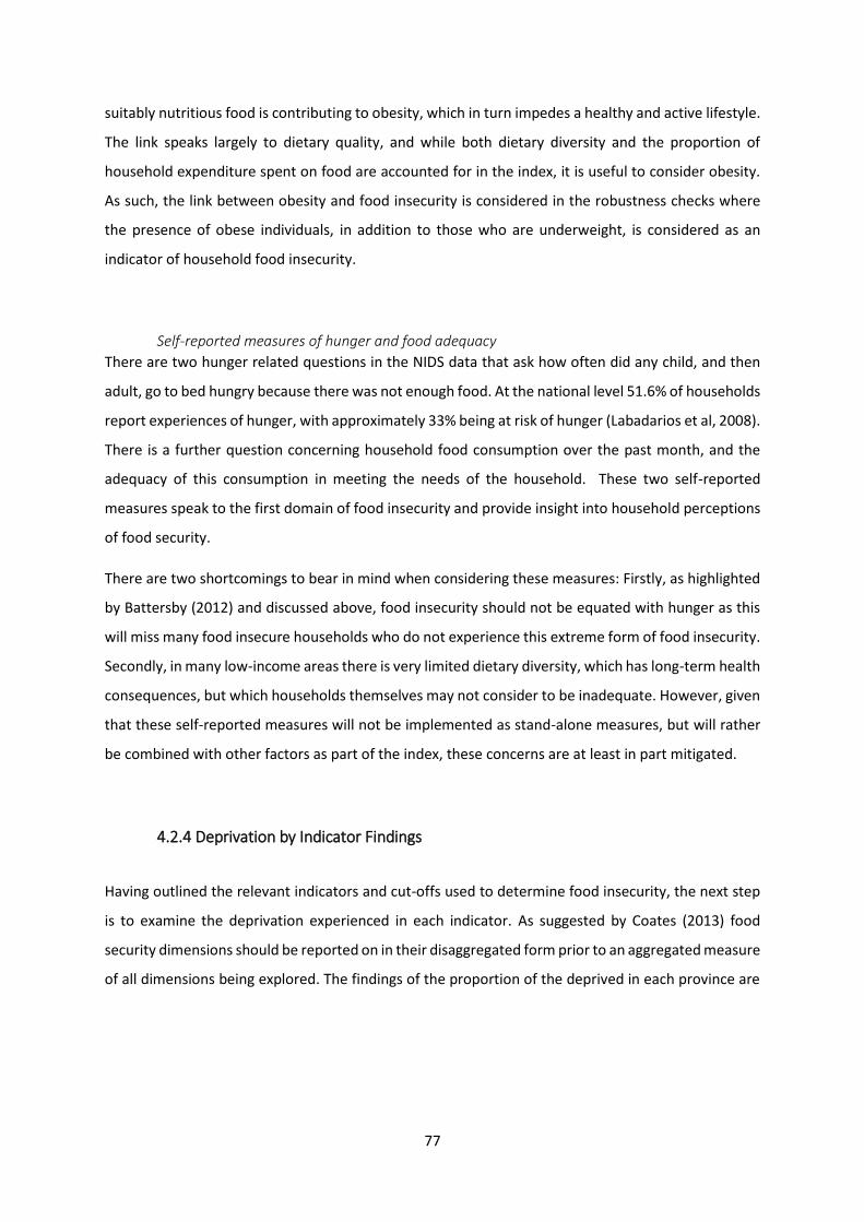
77
suitably nutritious food is contributing to obesity, which in turn impedes a healthy and active lifestyle.
The link speaks largely to dietary quality, and while both dietary diversity and the proportion of
household expenditure spent on food are accounted for in the index, it is useful to consider obesity.
As such, the link between obesity and food insecurity is considered in the robustness checks where
the presence of obese individuals, in addition to those who are underweight, is considered as an
indicator of household food insecurity.
Self-reported measures of hunger and food adequacy
There are two hunger related questions in the NIDS data that ask how often did any child, and then
adult, go to bed hungry because there was not enough food. At the national level 51.6% of households
report experiences of hunger, with approximately 33% being at risk of hunger (Labadarios et al, 2008).
There is a further question concerning household food consumption over the past month, and the
adequacy of this consumption in meeting the needs of the household. These two self-reported
measures speak to the first domain of food insecurity and provide insight into household perceptions
of food security.
There are two shortcomings to bear in mind when considering these measures: Firstly, as highlighted
by Battersby (2012) and discussed above, food insecurity should not be equated with hunger as this
will miss many food insecure households who do not experience this extreme form of food insecurity.
Secondly, in many low-income areas there is very limited dietary diversity, which has long-term health
consequences, but which households themselves may not consider to be inadequate. However, given
that these self-reported measures will not be implemented as stand-alone measures, but will rather
be combined with other factors as part of the index, these concerns are at least in part mitigated.
4.2.4 Deprivation by Indicator Findings
Having outlined the relevant indicators and cut-offs used to determine food insecurity, the next step
is to examine the deprivation experienced in each indicator. As suggested by Coates (2013) food
security dimensions should be reported on in their disaggregated form prior to an aggregated measure
of all dimensions being explored. The findings of the proportion of the deprived in each province are
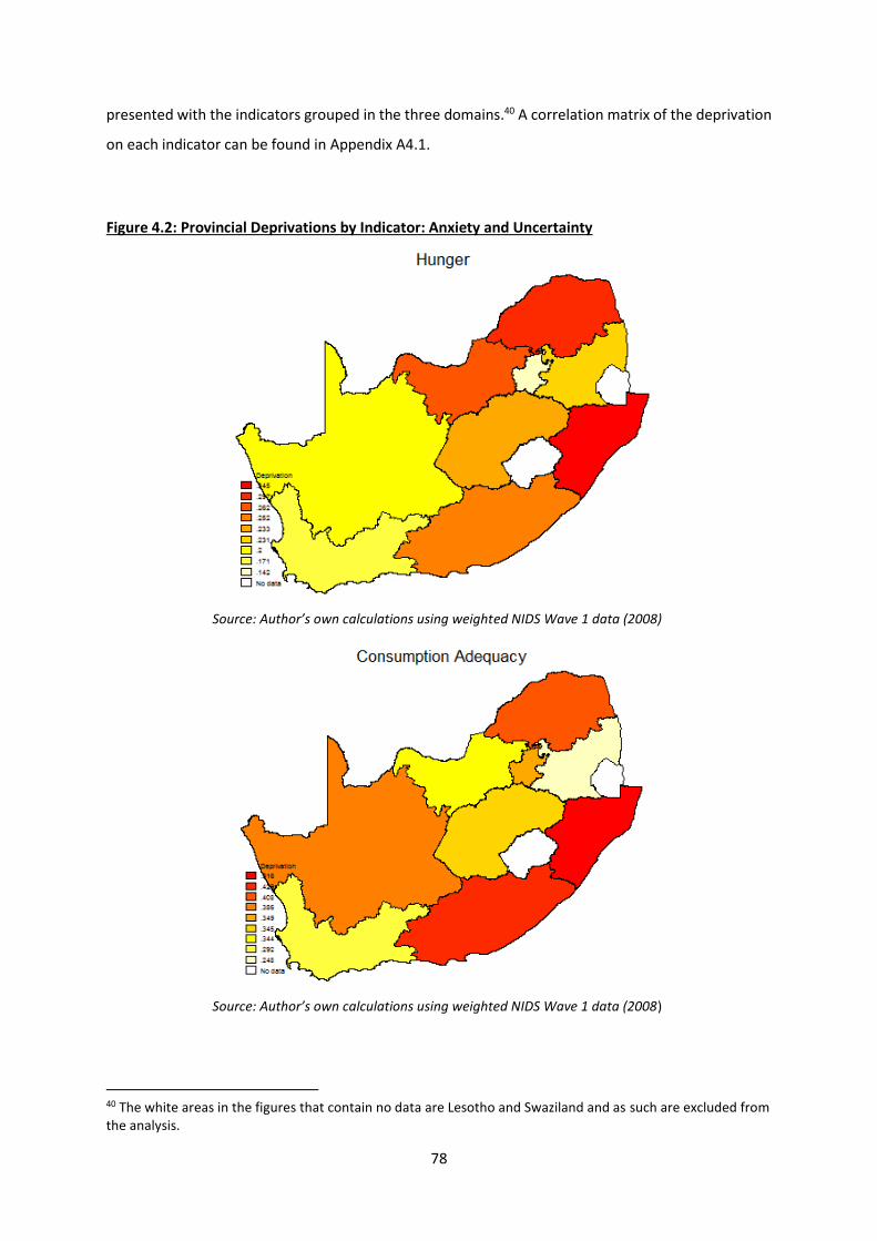
78
presented with the indicators grouped in the three domains.40 A correlation matrix of the deprivation
on each indicator can be found in Appendix A4.1.
Figure 4.2: Provincial Deprivations by Indicator: Anxiety and Uncertainty
Source: Author’s own calculations using weighted NIDS Wave 1 data (2008)
Source: Author’s own calculations using weighted NIDS Wave 1 data (2008)
40 The white areas in the figures that contain no data are Lesotho and Swaziland and as such are excluded from the analysis.
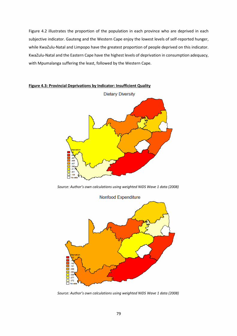
79
Figure 4.2 illustrates the proportion of the population in each province who are deprived in each
subjective indicator. Gauteng and the Western Cape enjoy the lowest levels of self-reported hunger,
while KwaZulu-Natal and Limpopo have the greatest proportion of people deprived on this indicator.
KwaZulu-Natal and the Eastern Cape have the highest levels of deprivation in consumption adequacy,
with Mpumalanga suffering the least, followed by the Western Cape.
Figure 4.3: Provincial Deprivations by Indicator: Insufficient Quality
Source: Author’s own calculations using weighted NIDS Wave 1 data (2008)
Source: Author’s own calculations using weighted NIDS Wave 1 data (2008)
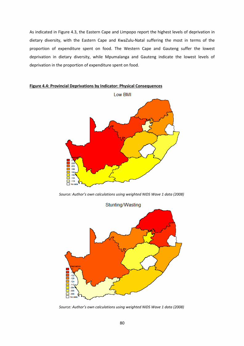
80
As indicated in Figure 4.3, the Eastern Cape and Limpopo report the highest levels of deprivation in
dietary diversity, with the Eastern Cape and KwaZulu-Natal suffering the most in terms of the
proportion of expenditure spent on food. The Western Cape and Gauteng suffer the lowest
deprivation in dietary diversity, while Mpumalanga and Gauteng indicate the lowest levels of
deprivation in the proportion of expenditure spent on food.
Figure 4.4: Provincial Deprivations by Indicator: Physical Consequences
Source: Author’s own calculations using weighted NIDS Wave 1 data (2008)
Source: Author’s own calculations using weighted NIDS Wave 1 data (2008)
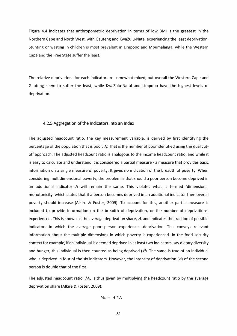
81
Figure 4.4 indicates that anthropometric deprivation in terms of low BMI is the greatest in the
Northern Cape and North West, with Gauteng and KwaZulu-Natal experiencing the least deprivation.
Stunting or wasting in children is most prevalent in Limpopo and Mpumalanga, while the Western
Cape and the Free State suffer the least.
The relative deprivations for each indicator are somewhat mixed, but overall the Western Cape and
Gauteng seem to suffer the least, while KwaZulu-Natal and Limpopo have the highest levels of
deprivation.
4.2.5 Aggregation of the Indicators into an Index
The adjusted headcount ratio, the key measurement variable, is derived by first identifying the
percentage of the population that is poor, H. That is the number of poor identified using the dual cut-
off approach. The adjusted headcount ratio is analogous to the income headcount ratio, and while it
is easy to calculate and understand it is considered a partial measure - a measure that provides basic
information on a single measure of poverty. It gives no indication of the breadth of poverty. When
considering multidimensional poverty, the problem is that should a poor person become deprived in
an additional indicator H will remain the same. This violates what is termed ‘dimensional
monotonicity’ which states that if a person becomes deprived in an additional indicator then overall
poverty should increase (Alkire & Foster, 2009). To account for this, another partial measure is
included to provide information on the breadth of deprivation, or the number of deprivations,
experienced. This is known as the average deprivation share, A, and indicates the fraction of possible
indicators in which the average poor person experiences deprivation. This conveys relevant
information about the multiple dimensions in which poverty is experienced. In the food security
context for example, if an individual is deemed deprived in at least two indicators, say dietary diversity
and hunger, this individual is then counted as being deprived (H). The same is true of an individual
who is deprived in four of the six indicators. However, the intensity of deprivation (A) of the second
person is double that of the first.
The adjusted headcount ratio, M0, is thus given by multiplying the headcount ratio by the average
deprivation share (Alkire & Foster, 2009):
M0 = H * A
82
M0 is sensitive to the frequency and the breadth of multidimensional poverty. Should either the
proportion of poor people, H, increase or the average number of dimensions in which the poor are
deprived, A, increase the adjusted headcount ratio will increase. The adjusted headcount ratio is one
of several multidimensional poverty measures that can be developed following this methodology.
Within the general Alkire-Foster framework, the adjusted headcount ratio can be calculated using any
dimensions, weights, and cut-offs, as determined by the question of interest.
In the general poverty literature, the MPI is a special case of the adjusted headcount ratio, in that it
makes use of specific indicators, cut-offs, and weights. The three dimensions are health, education
and living standards, with a few indicators for each. The indicators are nutrition, child mortality, years
of schooling, school attendance, cooking fuel, sanitation, water and electricity, floor type, and assets.
Each dimension and each indicator within the dimensions is equally weighted. The within dimension
cut-offs are guided by the literature, and the cross-dimensional cut-off is set at 2/6.41 These specific
choices make the MPI one of many possible applications of the Alkire-Foster multidimensional
methodology to poverty. A different index might use different indicators, weights and/or cut-offs. It
is exactly this generalisability of the framework that makes the method applicable to the food security
context, where the dimensions and indicators chosen are specific to the measurement of food
insecurity.
It is worth highlighting the methodological point that the ‘censoring’ step is key to the identification
process. This censoring means that the aggregate measure only includes deprivation information of
the poor, and not those who may be deprived in a single dimension but are not identified as poor. This
is important because information on the deprivations of the non-poor should not affect any measure
that is focused on the poor (Alkire & Foster, 2011).
The choice of the dimensions, weights, and cut-offs are key aspects of the index and require further
discussion. The dimensions chosen, and the cut-offs within each, are largely guided by the literature
where a general motivation and interpretation can be found for each indicator of interest. Selecting
these can also be determined by the availability of data to some extent (Alkire & Santos, 2010). In
contrast, the cross-dimensional cut-off is less directed by the literature, and can rely on several points.
For example, the minimum deprivation count required to be considered poor in a specific context,
where the cut-off could be set to the minimal level of one if deprivation on any one dimension is
considered a gross violation. Alternatively, it might be guided by specific policy goals and priorities,
where changing the cut-off can allow for the analysis of a smaller group with multiple deprivations, or
41 For the details of the MPI dimensions, weights, and cut-offs see Alkire & Santos (2010)
83
a wider group with fewer. It is advised that any choice of cut-off is tested for robustness (Alkire &
Foster, 2009).
By defining a measurement based on deprivation counts and simple averages, an equal weight is
implicitly assigned to each dimension of the MPI (Alkire & Foster, 2009). The interpretation of the
indicators is also made easier by assigning equal, or at least not very different, degrees of importance
to the different indicators (Atkinson, Cantillion, Marlier & Nolan, 2002). While this is appropriate when
the dimensions have been chosen to be of equal importance, it is no longer applicable when there is
reason to believe that some indicators are more important, or bear more weight, than others. The
choice of equal weights does not go uncontested. It is however noted by Foster & Sen (1997) that the
selection of weights is a judgemental exercise, only resolved through reasoned evaluation. While they
should enjoy reasonable acceptance, it is important that the dimensional weights used are open to
criticism. The issue of weights will be considered in more detail in the Robustness section.
Considering that there is no a priori reason to believe otherwise, and for ease of interpretation, each
dimension of the MFII is equally weighted, and each indicator within the dimensions is also equally
weighted. There does not appear to be any indication in the literature that the weights should be
anything different, but as suggested for the weights in the MPI context these will be varied as part of
the robustness checks.42 Each indicator has its own cut-off point which determines whether a
household or individual is food insecure in that measure. These cut-offs are guided by the literature
and have been discussed in detail. The second cut-off, the cross-dimensional cut-off, stipulates that a
person is identified as food insecure if he/she isdeprived in at least one third, or 2 of the 6, weighted
indicators. This again is based on the MPI method, and will be varied as part of the robustness tests.
4.2.6 Using the Decomposition Properties of the Index for Food Insecurity Analysis in
South Africa
Part of the value of such multidimensional measures is the unique properties which allow for a
detailed analysis of the problem. These include the decomposability of the index, and the ability to
calculate the percentage contribution of each indicator to the overall measure. The property of
decomposability requires overall poverty to be the weighted average of subgroup poverty levels,
where weights are subgroup population shares, and ensures that poverty is evaluated relative to the
42 This will include a brief discussion on the relative importance of subjective versus objective measures of food insecurity.
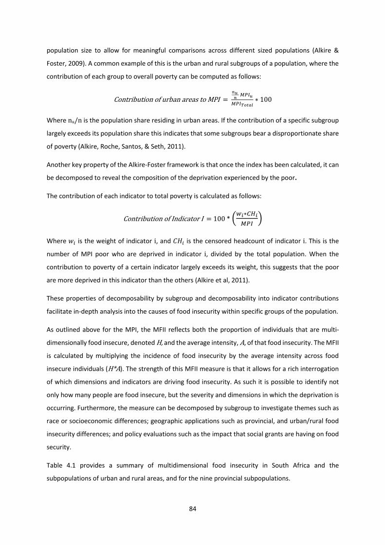
84
population size to allow for meaningful comparisons across different sized populations (Alkire &
Foster, 2009). A common example of this is the urban and rural subgroups of a population, where the
contribution of each group to overall poverty can be computed as follows:
Contribution of urban areas to MPI = 𝑛𝑢
𝑛 𝑀𝑃𝐼𝑢
𝑀𝑃𝐼𝑇𝑜𝑡𝑎𝑙∗ 100
Where nu/n is the population share residing in urban areas. If the contribution of a specific subgroup
largely exceeds its population share this indicates that some subgroups bear a disproportionate share
of poverty (Alkire, Roche, Santos, & Seth, 2011).
Another key property of the Alkire-Foster framework is that once the index has been calculated, it can
be decomposed to reveal the composition of the deprivation experienced by the poor.
The contribution of each indicator to total poverty is calculated as follows:
Contribution of Indicator I = 100 * (𝑤𝑖∗𝐶𝐻𝑖
𝑀𝑃𝐼)
Where 𝑤𝑖 is the weight of indicator i, and 𝐶𝐻𝑖 is the censored headcount of indicator i. This is the
number of MPI poor who are deprived in indicator i, divided by the total population. When the
contribution to poverty of a certain indicator largely exceeds its weight, this suggests that the poor
are more deprived in this indicator than the others (Alkire et al, 2011).
These properties of decomposability by subgroup and decomposability into indicator contributions
facilitate in-depth analysis into the causes of food insecurity within specific groups of the population.
As outlined above for the MPI, the MFII reflects both the proportion of individuals that are multi-
dimensionally food insecure, denoted H, and the average intensity, A, of that food insecurity. The MFII
is calculated by multiplying the incidence of food insecurity by the average intensity across food
insecure individuals (H*A). The strength of this MFII measure is that it allows for a rich interrogation
of which dimensions and indicators are driving food insecurity. As such it is possible to identify not
only how many people are food insecure, but the severity and dimensions in which the deprivation is
occurring. Furthermore, the measure can be decomposed by subgroup to investigate themes such as
race or socioeconomic differences; geographic applications such as provincial, and urban/rural food
insecurity differences; and policy evaluations such as the impact that social grants are having on food
security.
Table 4.1 provides a summary of multidimensional food insecurity in South Africa and the
subpopulations of urban and rural areas, and for the nine provincial subpopulations.
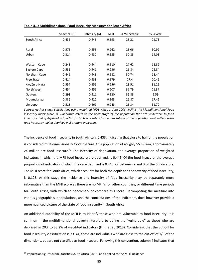
85
Table 4.1: Multidimensional Food Insecurity Measures for South Africa
Incidence (H) Intensity (A) MFII % Vulnerable % Severe
South Africa 0.433 0.445 0.193 28.21 21.71
Rural 0.576 0.455 0.262 25.06 30.92
Urban 0.314 0.430 0.135 30.85 14.03
Western Cape 0.248 0.444 0.110 27.62 12.82
Eastern Cape 0.535 0.441 0.236 26.84 26.84
Northern Cape 0.441 0.443 0.182 30.74 18.44
Free State 0.414 0.433 0.179 27.4 20.46
KwaZulu-Natal 0.557 0.459 0.256 23.51 31.25
North West 0.454 0.456 0.207 31.79 21.37
Gauteng 0.293 0.411 0.120 35.88 9.59
Mpumalanga 0.386 0.422 0.163 26.87 17.42
Limpopo 0.518 0.469 0.243 23.34 31.70
Source: Author’s own calculations using weighted NIDS Wave 1 data 2008. MFII is the Multidimensional Food
Insecurity Index score. % Vulnerable refers to the percentage of the population that are vulnerable to food
insecurity, being deprived in 1 indicator. % Severe refers to the percentage of the population that suffer severe
food insecurity, being deprived in 3 or more indicators.
The incidence of food insecurity in South Africa is 0.433, indicating that close to half of the population
is considered multidimensionally food insecure. Of a population of roughly 55 million, approximately
24 million are food insecure.43 The intensity of deprivation, the average proportion of weighted
indicators in which the MFII food insecure are deprived, is 0.445. Of the food insecure, the average
proportion of indicators in which they are deprived is 0.445, or between 2 and 3 of the 6 indicators.
The MFII score for South Africa, which accounts for both the depth and the severity of food insecurity,
is 0.193. At this stage the incidence and intensity of food insecurity may be separately more
informative than the MFII score as there are no MFII’s for other countries, or different time periods
for South Africa, with which to benchmark or compare this score. Decomposing the measure into
various geographic subpopulations, and the contributions of the indicators, does however provide a
more nuanced picture of the state of food insecurity in South Africa.
An additional capability of the MFII is to identify those who are vulnerable to food insecurity. It is
common in the multidimensional poverty literature to define the “vulnerable” as those who are
deprived in 20% to 33.2% of weighted indicators (Finn et al, 2013). Considering that the cut-off for
food insecurity classification is 33.3%, these are individuals who are close to the cut-off of 1/3 of the
dimensions, but are not classified as food insecure. Following this convention, column 4 indicates that
43 Population figures from Statistics South Africa (2015) and applied to the MFII incidence
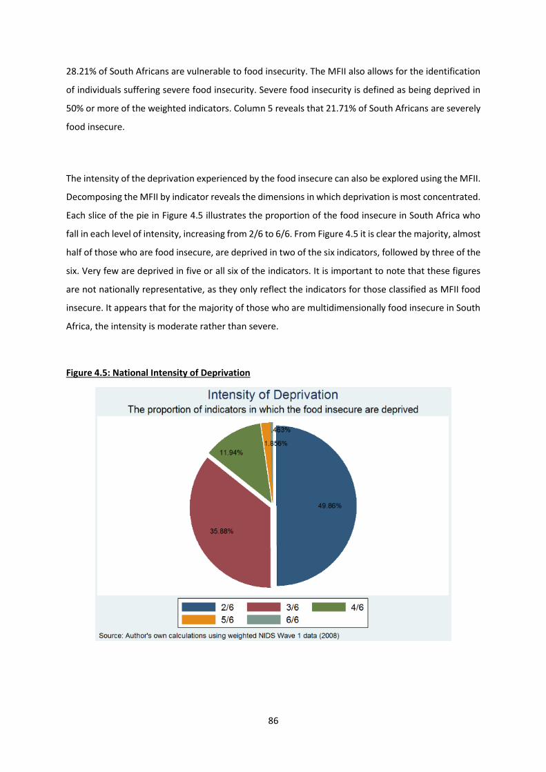
86
28.21% of South Africans are vulnerable to food insecurity. The MFII also allows for the identification
of individuals suffering severe food insecurity. Severe food insecurity is defined as being deprived in
50% or more of the weighted indicators. Column 5 reveals that 21.71% of South Africans are severely
food insecure.
The intensity of the deprivation experienced by the food insecure can also be explored using the MFII.
Decomposing the MFII by indicator reveals the dimensions in which deprivation is most concentrated.
Each slice of the pie in Figure 4.5 illustrates the proportion of the food insecure in South Africa who
fall in each level of intensity, increasing from 2/6 to 6/6. From Figure 4.5 it is clear the majority, almost
half of those who are food insecure, are deprived in two of the six indicators, followed by three of the
six. Very few are deprived in five or all six of the indicators. It is important to note that these figures
are not nationally representative, as they only reflect the indicators for those classified as MFII food
insecure. It appears that for the majority of those who are multidimensionally food insecure in South
Africa, the intensity is moderate rather than severe.
Figure 4.5: National Intensity of Deprivation
87
A further step in unpacking multidimensional food insecurity is to analyse the contributions of each
indicator to the overall MFII measure. Figure 4.6 reveals that the two largest contributors to
multidimensional food insecurity in South Africa are poor dietary diversity and the subjective
perception of consumption adequacy. These are followed by self-reported hunger. Low BMI, stunting
and wasting, and non-food expenditure make up smaller proportions. The prominence of the
subjective measures of food insecurity, self-reported consumption adequacy and self-reported
hunger, in the top three contributors is worth noting. While dietary diversity, an objective measure, is
the largest contributor, these subjective measures are certainly prominent. This emphasises the
importance of examining and understanding the differences between subjective and objective
measures, their relative importance, and what they mean for the measurement of food insecurity. As
mentioned previously, the methodology allows for varying the emphasis placed on subjective versus
objective measures by changing the weights applied as illustrated in the Robustness section.
Figure 4.6: Indicator Contributions to National MFII
Contributions to the MFII for South Africa can also be calculated for geographic areas. Figures 4.7 and
4.8 show the contributions of each province to the national MFII score, and the contributions of urban
and rural areas. KwaZulu-Natal is the greatest contributor, accounting for more than a quarter of the
national MFII figure at 29.54%. The Northern Cape contributes the least to overall food insecurity at
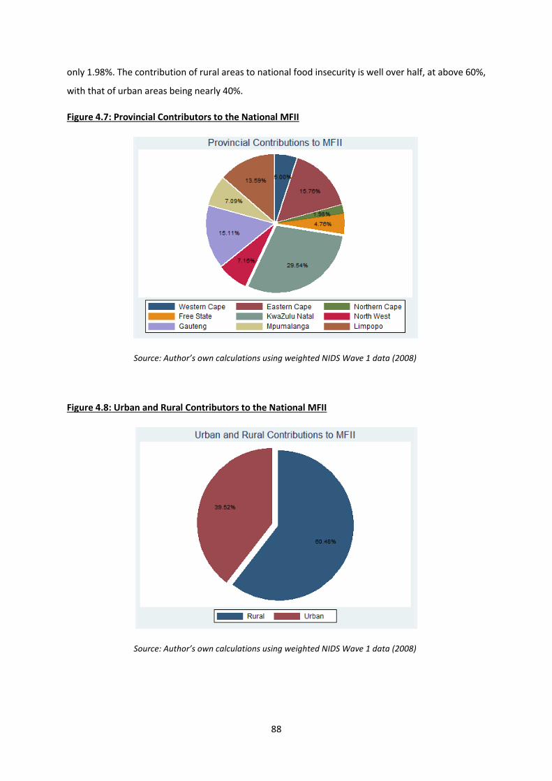
88
only 1.98%. The contribution of rural areas to national food insecurity is well over half, at above 60%,
with that of urban areas being nearly 40%.
Figure 4.7: Provincial Contributors to the National MFII
Source: Author’s own calculations using weighted NIDS Wave 1 data (2008)
Figure 4.8: Urban and Rural Contributors to the National MFII
Source: Author’s own calculations using weighted NIDS Wave 1 data (2008)

89
Rural and Urban Subpopulations
As indicated in Table 4.1, rural areas contain over one and a half times more MFII food insecure people
than urban areas, with incidences of 0.576 and 0.314 respectively. Furthermore, the intensity of food
insecurity experienced in rural areas is somewhat greater than that in urban areas at 0.455 and 0.430
respectively. Those suffering acute food insecurity are mostly concentrated in rural areas, as reflected
in the proportion of food insecure who are severely so, at 30.92%. These finding are not surprising,
and confirm other relative measures of food insecurity in South Africa highlighted in the introduction.
The strength of the MFII, however, is that it allows for detailed interrogation of which dimensions are
contributing the most to food insecurity in each area.
Provincial Subpopulations
Figure 4.9: Provincial Food Insecurity
Figure 4.9 illustrates the MFII scores for the nine provinces, and allows for easy identification of those
provinces with the highest levels of food insecurity. Those suffering the highest multidimensional food
insecurity are KwaZulu-Natal (0.256) and Limpopo (0.243). These provinces are largely rural, and this
is consistent with the findings for the rural/urban subpopulations. There are however other provinces
that are also largely rural but with lower MFII scores, indicating that there are other factors at play in
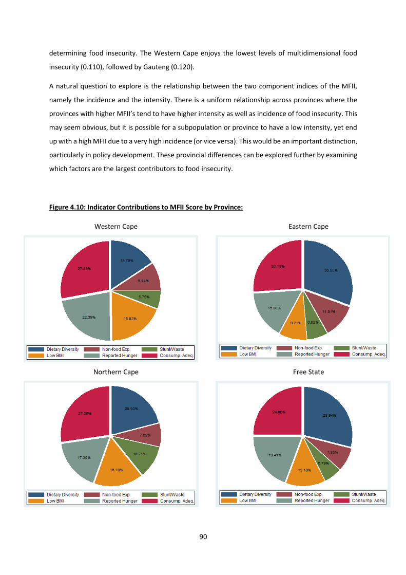
90
determining food insecurity. The Western Cape enjoys the lowest levels of multidimensional food
insecurity (0.110), followed by Gauteng (0.120).
A natural question to explore is the relationship between the two component indices of the MFII,
namely the incidence and the intensity. There is a uniform relationship across provinces where the
provinces with higher MFII’s tend to have higher intensity as well as incidence of food insecurity. This
may seem obvious, but it is possible for a subpopulation or province to have a low intensity, yet end
up with a high MFII due to a very high incidence (or vice versa). This would be an important distinction,
particularly in policy development. These provincial differences can be explored further by examining
which factors are the largest contributors to food insecurity.
Figure 4.10: Indicator Contributions to MFII Score by Province:
Western Cape
Eastern Cape
Northern Cape
Free State
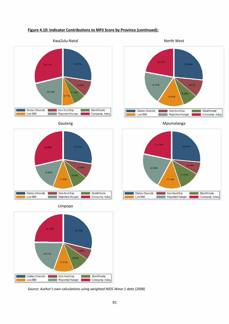
91
Figure 4.10: Indicator Contributions to MFII Score by Province (continued):
KwaZulu-Natal
North West
Gauteng
Mpumalanga
Limpopo
Source: Author’s own calculations using weighted NIDS Wave 1 data (2008)
92
Figure 4.10 reveals that the comparative contributions of each indicator to MFII by province reflect
those for the whole country, with dietary diversity and subjective consumption adequacy being the
greatest contributors. The Western Cape is the one exception, with self-reported hunger superseding
dietary diversity as one of the two greatest contributors. Thus, the two subjective measures of food
insecurity are the greatest contributors to food insecurity in the Western Cape. This is a potentially
interesting finding worth investigating further considering the potential differences between
subjective and objective measurement. These patterns are reflected in the proportion of the food
insecure deprived on each indicator, found in Appendix A4.2.
4.3 Robustness checks
In general, different methods of constructing food insecurity measures can lead to different
conclusions, thus it is necessary to include several robustness checks in any analysis (Hendriks, 2005).
More specifically the methodology of the MPI is not without its limitations and shortcomings, and it is
necessary to discuss and address these criticisms which also apply to the MFII. As noted by Foster
(2010) this methodology is best seen as a general framework for measuring multidimensional poverty
where most of the hard decisions are left to the user. These ‘hard decisions’ include the selection of
dimensional weights, dimensional cut-offs, and a poverty cut-off. The MFII construction also relies on
these decisions, and robustness tests are required to test the sensitivity of the measure to these
choices. Alkire, Foster and others, are open and forthcoming about these issues, and promote
discussion and debate of these topics.44
The bulk of the MPI debate is centred on the issue of weights and the imbedded trade-offs. A leading
critic aptly puts this concern as “the index is essentially adding up ‘apples and oranges’ without
knowing their relative price” (Ravallion, 2010). This stems from indicators being weighted essentially
arbitrarily in the construction of the index. For the MPI this results in equating the death of a child
with having a dirt floor and cooking with wood, in terms of the weight each indicator bears. The MFII
does not include any extreme dimensions such as this. Equating self-reported hunger with under-
nourishment is arguably not as problematic as equating the death of a child with cooking fuel. The
lack of theory to support the chosen weightings in the MPI does however extend to the MFII, but as
pointed out by Alkire (2010) a lack of theory should not mean that no weighting be given at all. Taking
44 See Alkire & Foster, 2011, and Alkire & Santos, 2010 for detailed discussions of these issues and how they can be addressed.
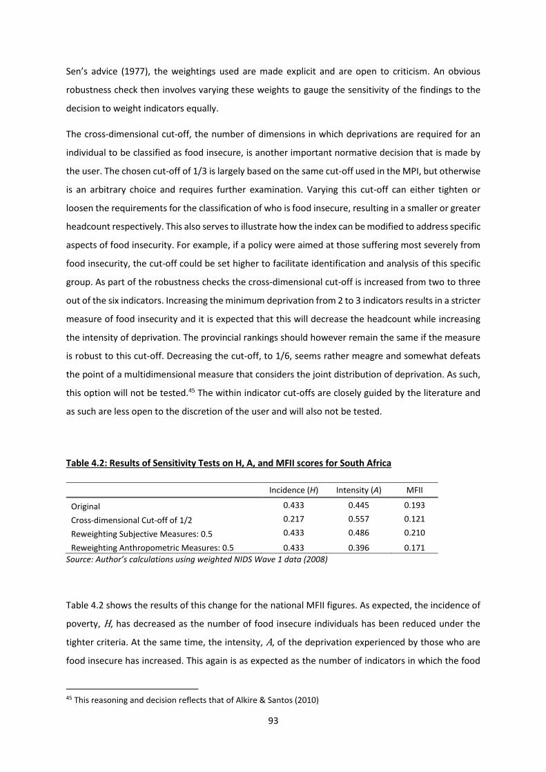
93
Sen’s advice (1977), the weightings used are made explicit and are open to criticism. An obvious
robustness check then involves varying these weights to gauge the sensitivity of the findings to the
decision to weight indicators equally.
The cross-dimensional cut-off, the number of dimensions in which deprivations are required for an
individual to be classified as food insecure, is another important normative decision that is made by
the user. The chosen cut-off of 1/3 is largely based on the same cut-off used in the MPI, but otherwise
is an arbitrary choice and requires further examination. Varying this cut-off can either tighten or
loosen the requirements for the classification of who is food insecure, resulting in a smaller or greater
headcount respectively. This also serves to illustrate how the index can be modified to address specific
aspects of food insecurity. For example, if a policy were aimed at those suffering most severely from
food insecurity, the cut-off could be set higher to facilitate identification and analysis of this specific
group. As part of the robustness checks the cross-dimensional cut-off is increased from two to three
out of the six indicators. Increasing the minimum deprivation from 2 to 3 indicators results in a stricter
measure of food insecurity and it is expected that this will decrease the headcount while increasing
the intensity of deprivation. The provincial rankings should however remain the same if the measure
is robust to this cut-off. Decreasing the cut-off, to 1/6, seems rather meagre and somewhat defeats
the point of a multidimensional measure that considers the joint distribution of deprivation. As such,
this option will not be tested.45 The within indicator cut-offs are closely guided by the literature and
as such are less open to the discretion of the user and will also not be tested.
Table 4.2: Results of Sensitivity Tests on H, A, and MFII scores for South Africa
Incidence (H) Intensity (A) MFII
Original 0.433 0.445 0.193
Cross-dimensional Cut-off of 1/2 0.217 0.557 0.121
Reweighting Subjective Measures: 0.5 0.433 0.486 0.210
Reweighting Anthropometric Measures: 0.5 0.433 0.396 0.171
Source: Author’s calculations using weighted NIDS Wave 1 data (2008)
Table 4.2 shows the results of this change for the national MFII figures. As expected, the incidence of
poverty, H, has decreased as the number of food insecure individuals has been reduced under the
tighter criteria. At the same time, the intensity, A, of the deprivation experienced by those who are
food insecure has increased. This again is as expected as the number of indicators in which the food
45 This reasoning and decision reflects that of Alkire & Santos (2010)
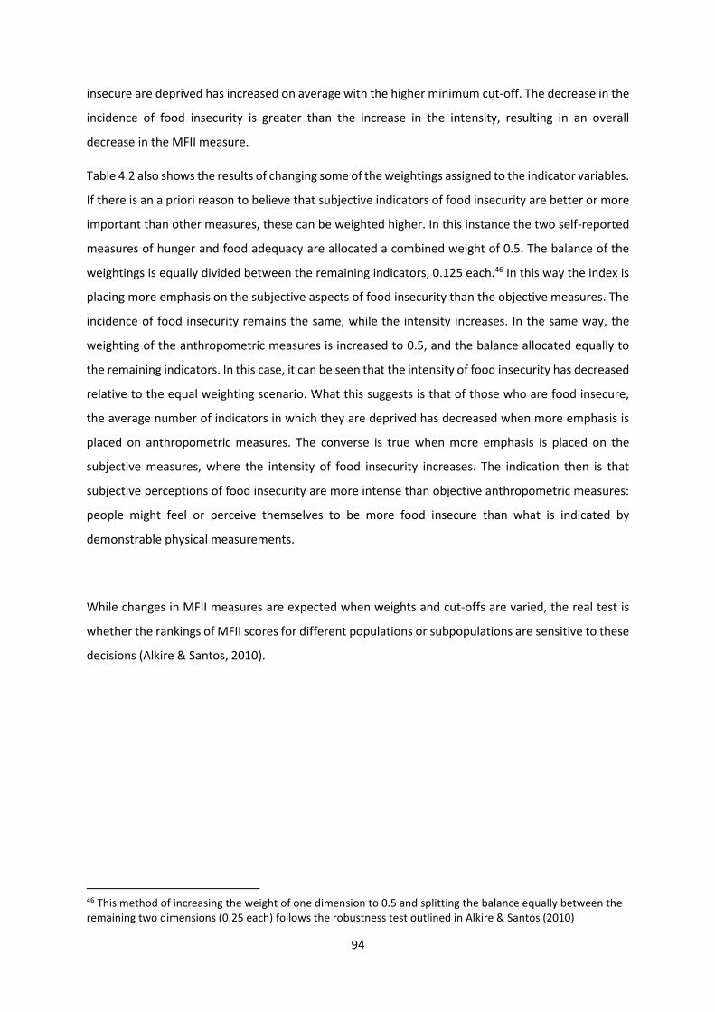
94
insecure are deprived has increased on average with the higher minimum cut-off. The decrease in the
incidence of food insecurity is greater than the increase in the intensity, resulting in an overall
decrease in the MFII measure.
Table 4.2 also shows the results of changing some of the weightings assigned to the indicator variables.
If there is an a priori reason to believe that subjective indicators of food insecurity are better or more
important than other measures, these can be weighted higher. In this instance the two self-reported
measures of hunger and food adequacy are allocated a combined weight of 0.5. The balance of the
weightings is equally divided between the remaining indicators, 0.125 each.46 In this way the index is
placing more emphasis on the subjective aspects of food insecurity than the objective measures. The
incidence of food insecurity remains the same, while the intensity increases. In the same way, the
weighting of the anthropometric measures is increased to 0.5, and the balance allocated equally to
the remaining indicators. In this case, it can be seen that the intensity of food insecurity has decreased
relative to the equal weighting scenario. What this suggests is that of those who are food insecure,
the average number of indicators in which they are deprived has decreased when more emphasis is
placed on anthropometric measures. The converse is true when more emphasis is placed on the
subjective measures, where the intensity of food insecurity increases. The indication then is that
subjective perceptions of food insecurity are more intense than objective anthropometric measures:
people might feel or perceive themselves to be more food insecure than what is indicated by
demonstrable physical measurements.
While changes in MFII measures are expected when weights and cut-offs are varied, the real test is
whether the rankings of MFII scores for different populations or subpopulations are sensitive to these
decisions (Alkire & Santos, 2010).
46 This method of increasing the weight of one dimension to 0.5 and splitting the balance equally between the remaining two dimensions (0.25 each) follows the robustness test outlined in Alkire & Santos (2010)
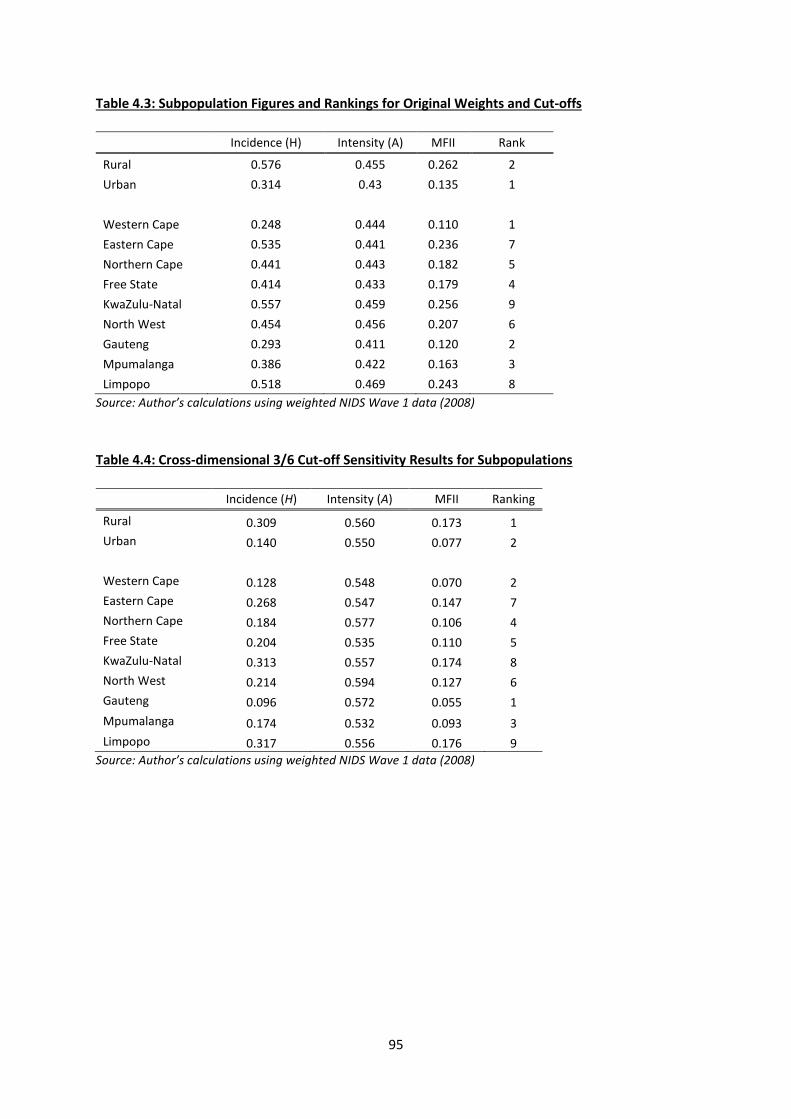
95
Table 4.3: Subpopulation Figures and Rankings for Original Weights and Cut-offs
Incidence (H) Intensity (A) MFII Rank
Rural 0.576 0.455 0.262 2
Urban 0.314 0.43 0.135 1
Western Cape 0.248 0.444 0.110 1
Eastern Cape 0.535 0.441 0.236 7
Northern Cape 0.441 0.443 0.182 5
Free State 0.414 0.433 0.179 4
KwaZulu-Natal 0.557 0.459 0.256 9
North West 0.454 0.456 0.207 6
Gauteng 0.293 0.411 0.120 2
Mpumalanga 0.386 0.422 0.163 3
Limpopo 0.518 0.469 0.243 8
Source: Author’s calculations using weighted NIDS Wave 1 data (2008)
Table 4.4: Cross-dimensional 3/6 Cut-off Sensitivity Results for Subpopulations
Incidence (H) Intensity (A) MFII Ranking
Rural 0.309 0.560 0.173 1
Urban 0.140 0.550 0.077 2
Western Cape 0.128 0.548 0.070 2
Eastern Cape 0.268 0.547 0.147 7
Northern Cape 0.184 0.577 0.106 4
Free State 0.204 0.535 0.110 5
KwaZulu-Natal 0.313 0.557 0.174 8
North West 0.214 0.594 0.127 6
Gauteng 0.096 0.572 0.055 1
Mpumalanga 0.174 0.532 0.093 3
Limpopo 0.317 0.556 0.176 9
Source: Author’s calculations using weighted NIDS Wave 1 data (2008)
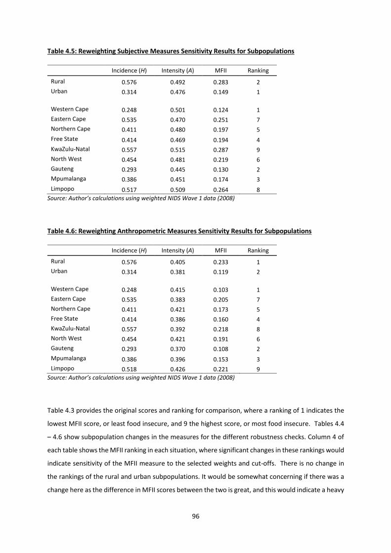
96
Table 4.5: Reweighting Subjective Measures Sensitivity Results for Subpopulations
Incidence (H) Intensity (A) MFII Ranking
Rural 0.576 0.492 0.283 2
Urban 0.314 0.476 0.149 1 Western Cape 0.248 0.501 0.124 1
Eastern Cape 0.535 0.470 0.251 7
Northern Cape 0.411 0.480 0.197 5
Free State 0.414 0.469 0.194 4
KwaZulu-Natal 0.557 0.515 0.287 9
North West 0.454 0.481 0.219 6
Gauteng 0.293 0.445 0.130 2
Mpumalanga 0.386 0.451 0.174 3
Limpopo 0.517 0.509 0.264 8
Source: Author’s calculations using weighted NIDS Wave 1 data (2008)
Table 4.6: Reweighting Anthropometric Measures Sensitivity Results for Subpopulations
Incidence (H) Intensity (A) MFII Ranking
Rural 0.576 0.405 0.233 1
Urban 0.314 0.381 0.119 2 Western Cape 0.248 0.415 0.103 1
Eastern Cape 0.535 0.383 0.205 7
Northern Cape 0.411 0.421 0.173 5
Free State 0.414 0.386 0.160 4
KwaZulu-Natal 0.557 0.392 0.218 8
North West 0.454 0.421 0.191 6
Gauteng 0.293 0.370 0.108 2
Mpumalanga 0.386 0.396 0.153 3
Limpopo 0.518 0.426 0.221 9
Source: Author’s calculations using weighted NIDS Wave 1 data (2008)
Table 4.3 provides the original scores and ranking for comparison, where a ranking of 1 indicates the
lowest MFII score, or least food insecure, and 9 the highest score, or most food insecure. Tables 4.4
– 4.6 show subpopulation changes in the measures for the different robustness checks. Column 4 of
each table shows the MFII ranking in each situation, where significant changes in these rankings would
indicate sensitivity of the MFII measure to the selected weights and cut-offs. There is no change in
the rankings of the rural and urban subpopulations. It would be somewhat concerning if there was a
change here as the difference in MFII scores between the two is great, and this would indicate a heavy
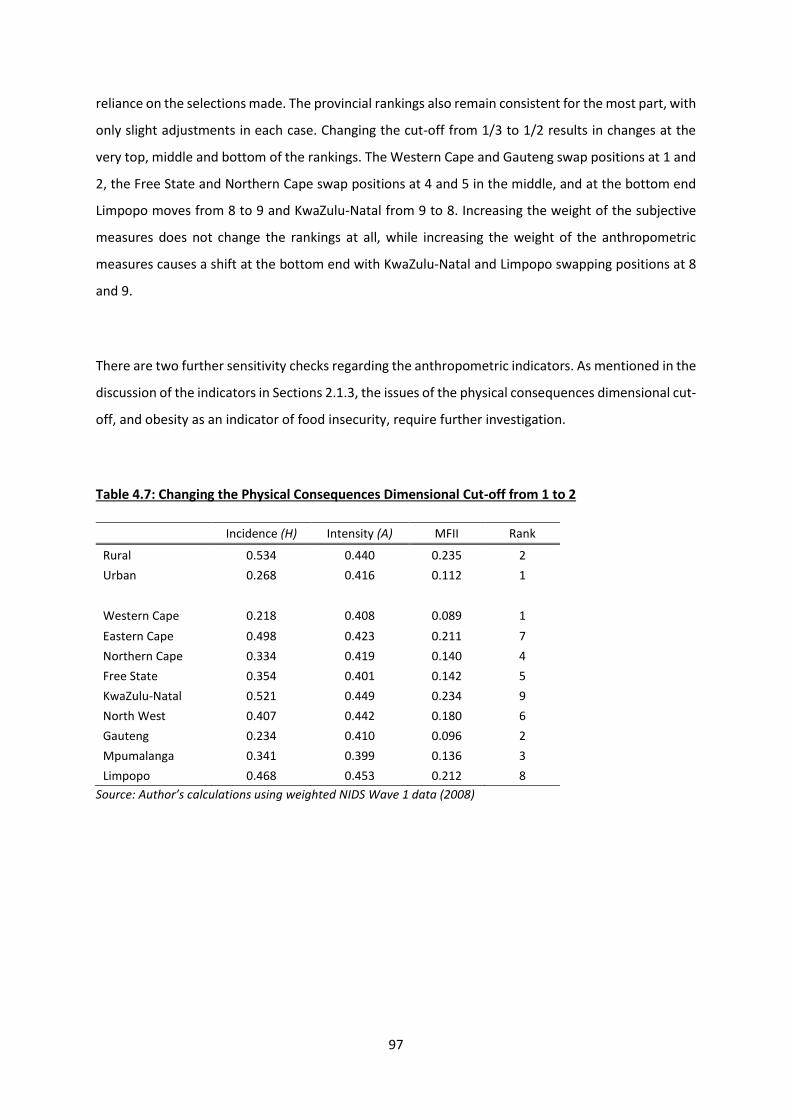
97
reliance on the selections made. The provincial rankings also remain consistent for the most part, with
only slight adjustments in each case. Changing the cut-off from 1/3 to 1/2 results in changes at the
very top, middle and bottom of the rankings. The Western Cape and Gauteng swap positions at 1 and
2, the Free State and Northern Cape swap positions at 4 and 5 in the middle, and at the bottom end
Limpopo moves from 8 to 9 and KwaZulu-Natal from 9 to 8. Increasing the weight of the subjective
measures does not change the rankings at all, while increasing the weight of the anthropometric
measures causes a shift at the bottom end with KwaZulu-Natal and Limpopo swapping positions at 8
and 9.
There are two further sensitivity checks regarding the anthropometric indicators. As mentioned in the
discussion of the indicators in Sections 2.1.3, the issues of the physical consequences dimensional cut-
off, and obesity as an indicator of food insecurity, require further investigation.
Table 4.7: Changing the Physical Consequences Dimensional Cut-off from 1 to 2
Incidence (H) Intensity (A) MFII Rank
Rural 0.534 0.440 0.235 2
Urban 0.268 0.416 0.112 1
Western Cape 0.218 0.408 0.089 1
Eastern Cape 0.498 0.423 0.211 7
Northern Cape 0.334 0.419 0.140 4
Free State 0.354 0.401 0.142 5
KwaZulu-Natal 0.521 0.449 0.234 9
North West 0.407 0.442 0.180 6
Gauteng 0.234 0.410 0.096 2
Mpumalanga 0.341 0.399 0.136 3
Limpopo 0.468 0.453 0.212 8
Source: Author’s calculations using weighted NIDS Wave 1 data (2008)
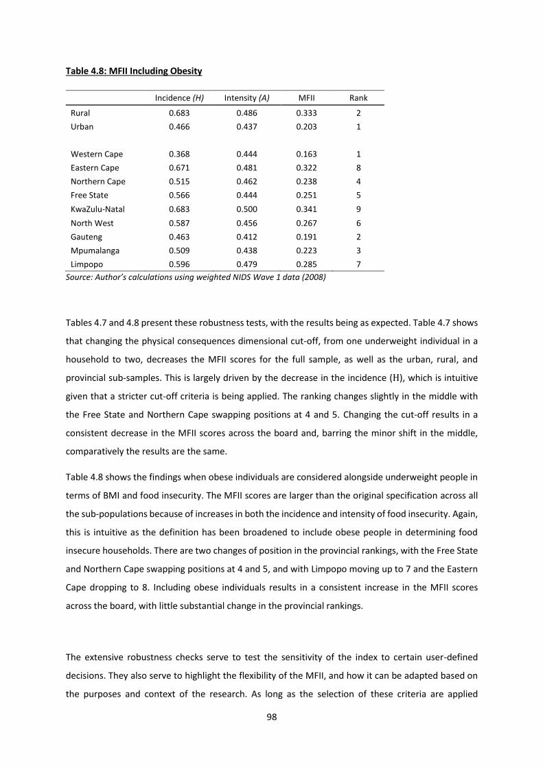
98
Table 4.8: MFII Including Obesity
Incidence (H) Intensity (A) MFII Rank
Rural 0.683 0.486 0.333 2
Urban 0.466 0.437 0.203 1
Western Cape 0.368 0.444 0.163 1
Eastern Cape 0.671 0.481 0.322 8
Northern Cape 0.515 0.462 0.238 4
Free State 0.566 0.444 0.251 5
KwaZulu-Natal 0.683 0.500 0.341 9
North West 0.587 0.456 0.267 6
Gauteng 0.463 0.412 0.191 2
Mpumalanga 0.509 0.438 0.223 3
Limpopo 0.596 0.479 0.285 7
Source: Author’s calculations using weighted NIDS Wave 1 data (2008)
Tables 4.7 and 4.8 present these robustness tests, with the results being as expected. Table 4.7 shows
that changing the physical consequences dimensional cut-off, from one underweight individual in a
household to two, decreases the MFII scores for the full sample, as well as the urban, rural, and
provincial sub-samples. This is largely driven by the decrease in the incidence (H), which is intuitive
given that a stricter cut-off criteria is being applied. The ranking changes slightly in the middle with
the Free State and Northern Cape swapping positions at 4 and 5. Changing the cut-off results in a
consistent decrease in the MFII scores across the board and, barring the minor shift in the middle,
comparatively the results are the same.
Table 4.8 shows the findings when obese individuals are considered alongside underweight people in
terms of BMI and food insecurity. The MFII scores are larger than the original specification across all
the sub-populations because of increases in both the incidence and intensity of food insecurity. Again,
this is intuitive as the definition has been broadened to include obese people in determining food
insecure households. There are two changes of position in the provincial rankings, with the Free State
and Northern Cape swapping positions at 4 and 5, and with Limpopo moving up to 7 and the Eastern
Cape dropping to 8. Including obese individuals results in a consistent increase in the MFII scores
across the board, with little substantial change in the provincial rankings.
The extensive robustness checks serve to test the sensitivity of the index to certain user-defined
decisions. They also serve to highlight the flexibility of the MFII, and how it can be adapted based on
the purposes and context of the research. As long as the selection of these criteria are applied
99
consistently to any food insecurity comparisons, the relative findings are not driven by these choices.
While there are some minor shifts in the provincial ranking, they do not represent fundamental
changes. The indication then is that the MFII measure is generally robust to the choices of weights and
cut-offs, with inconsequential deviations in ranking. While these choices can be adjusted by the user
based on the question of interest, the MFII does not appear to be heavily dependent on these
normative decisions. This is important in establishing the measure as a widely applicable and robust
food insecurity measure.
An additional issue raised about the Alkire-Foster method is the requirement of data from a single
survey, or at least matched surveys. This can result in sub-standard data being utilised in the
construction of the index if this is all that is available. This concern over data quality is not unique to
this methodology and is often an issue in quantitative research. However, with the scope and quality
of surveys, especially multi-topic surveys, constantly improving, this concern is likely to diminish. The
NIDS dataset is one of the few nationally representative datasets to include detailed food security
related question, and is widely considered a reliable source. The indicators used are well-documented
measures of food insecurity and not limited by the availability of data. No obvious measure or concept
from the literature has been excluded due to a lack of data. A data concern that does however persist
is that subsequent waves of the survey do not include all the indicators used in the construction of the
index. For the moment, this limits the possibility of monitoring food insecurity over time in South
Africa with a consistent MFII using NIDS data.
4.4 Policy Discussion and Conclusion
While considerable work has been done in developing multidimensional measures for poverty, less
has been done in terms of such a methodology for measuring multidimensional food insecurity. One
example of a multidimensional measure developed by Maxwell, Coates & Vaitla (2013) constructs a
multidimensional indicator, the Multidimensional Food Security Indicator (MFSI), using an algorithmic
approach. The method involves first empirically extracting categories using a network modularity
approach, and then refining these inductive results with theory. The MFII is arguably conceptually
easier to understand and calculate than the MFSI, and has useful properties for analysis that make it
a valuable tool for policy development. Furthermore, the methodology has already gained good
traction in the poverty measurement discourse.
100
Some attempts have also been made to aggregate the multiple dimensions of food insecurity into one
univariate index. An example of this is the Global Food Security Index developed by the Economist
Intelligence Unit.47 However indices such as these suffer from the same criticism as some poverty
indices - that of merely redefining food security while remaining unidimensional. For example, a
common unidimensional method for creating such a composite indicator is to aggregate across several
component variables by multiplying each by some factor, and adding up. Such methods however mean
that a shortfall in any one dimension is not of concern, as it can be completely compensated for by
gains in another dimension (Alkire & Foster, 2011). This results in the many dimensions being merged
into one, and when shortfalls in some dimensions are offset by excesses in others, information on the
individual impact of dimensions on the aggregate measure is lost. There is further apprehension about
the use of a single metric of food insecurity, with Coates (2013) highlighting the following issues: 1)
underestimation of food insecurity by overlooking the quantification of dimensions, 2) difficult
diagnostics obscuring potential causes and consequences of individual elements of food insecurity, 3)
diagnostic errors resulting in “one-size-fits-all” interventions, and 4) biased impact estimation of
interventions. These concerns are largely overcome by the methodology and properties of the MFII,
where no information on the various dimensions is lost through aggregation. Furthermore, the
decomposability of the index facilitates tailor-made interventions for specific sub-populations, as well
as detailed impact evaluation of specific indicators.
In terms of policy analysis, the MFII is a useful tool in both the development of new policies and the
evaluation of existing efforts. The decomposability property of the index also makes it particularly
valuable in crafting targeted household and individual food security policy. The ability to decompose
the MFII by subgroup means that the index score and major contributing indicators to food insecurity
can be identified for specific subgroups of interest. The provincial analysis presented is one example.
By examining food insecurity in this way, it is possible to identify those provinces suffering the greatest
levels of food insecurity. Not only can polices then be directed at these specific subgroups, but it is
also possible to target policies at those indicators that are the greatest contributors to food insecurity.
For example, KwaZulu-Natal and Limpopo are the most food insecure provinces, with subjective
consumption adequacy and dietary diversity being the greatest contributors. Policies can then be
directed at these two indicators in tackling the most pressing concerns.
47 Accessible from http://foodsecurityindex.eiu.com/
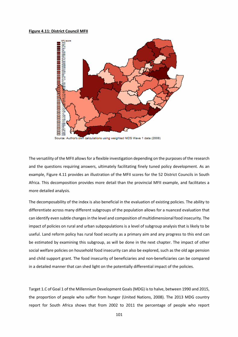
101
Figure 4.11: District Council MFII
The versatility of the MFII allows for a flexible investigation depending on the purposes of the research
and the questions requiring answers, ultimately facilitating finely tuned policy development. As an
example, Figure 4.11 provides an illustration of the MFII scores for the 52 District Councils in South
Africa. This decomposition provides more detail than the provincial MFII example, and facilitates a
more detailed analysis.
The decomposability of the index is also beneficial in the evaluation of existing policies. The ability to
differentiate across many different subgroups of the population allows for a nuanced evaluation that
can identify even subtle changes in the level and composition of multidimensional food insecurity. The
impact of policies on rural and urban subpopulations is a level of subgroup analysis that is likely to be
useful. Land reform policy has rural food security as a primary aim and any progress to this end can
be estimated by examining this subgroup, as will be done in the next chapter. The impact of other
social welfare policies on household food insecurity can also be explored, such as the old age pension
and child support grant. The food insecurity of beneficiaries and non-beneficiaries can be compared
in a detailed manner that can shed light on the potentially differential impact of the policies.
Target 1.C of Goal 1 of the Millennium Development Goals (MDG) is to halve, between 1990 and 2015,
the proportion of people who suffer from hunger (United Nations, 2008). The 2013 MDG country
report for South Africa shows that from 2002 to 2011 the percentage of people who report

102
experiencing hunger dropped from 29.9 to 12.9 (United Nations Development Programme, 2014).48
As such, South Africa is reported to have achieved target 1.C of halving the number of people suffering
from hunger. However, hunger is a limited measure of food insecurity that ignores many other
important factors (Battersby, 2012). A promising indication regarding this is that a key
recommendation highlighted in the report is the inclusion of additional measures to that of reported
hunger. These include dietary diversity, a child food security indicator, and other mixed methods of
data gathering such as anthropometric measurement. It appears then that South Africa recognises
food insecurity as a multidimensional phenomenon, requiring more detailed measurement than
simply counting the incidence of self-reported hunger.
The multidimensional nature of food insecurity is a given, and the “holy grail” of food security
measurement would be “a single measure that is valid and reliable, comparable over time and space,
and which captures different elements of food security” (Maxwell et al, pp 3; 2013). The MFII
presented here not only meets these criteria, but also includes other beneficial characteristics that
make it a useful tool for practical food insecurity analysis. When considering the development of a
multidimensional measure of food insecurity, a key consideration is whether there is anything to be
gained by adopting a multidimensional perspective.49 Implicit in this approach is that the use of a
single indicator is not a suitable or sufficient variable with which to measure the food insecurity status
of a household or individual. This chapter provides compelling evidence that such a composite
multidimensional food insecurity measure contributes to better thinking about food security, and
allows for the possibility of more targeted identification, and subsequently improved policies for
fighting food insecurity. A theoretical aim of the Alkire-Foster MPI measure was to re-examine the
identification step – addressing the question ‘who is poor’? (Foster & Santos, 2010). In the same vein,
answering the question of ‘who is food insecure’ is a fundamental question in this paper, and the
creation of a useful and insightful measure of this has been a key aim. The sensitivity tests, while
addressing some of the criticisms of the methodology, also serve to illustrate the flexibility of the
index. It can be adapted depending on the motivation, question, context, and prior beliefs, while
retaining all the properties that make it a useful tool for detailed analysis.
To a large extent, the results obtained for South Africa are intuitive, and do not contradict previous
findings. They are also significantly more detailed, and allow for more targeted analysis. In sum, 48.2%
of South Africans are considered multidimensionally food insecure, and 28.51% are severely so. A
48 Calculated using the General Household survey, Statistics South Africa 49 As noted by Tsui (2000) when considering a multidimensional approach for the measurement of poverty
103
further 25.77% of the population is vulnerable to food insecurity. Rural areas suffer greater intensity
and prevalence of food insecurity than urban areas, however the roughly equal contribution of each
area to national food insecurity indicates that urban areas require as much attention as rural areas.
Limpopo and KwaZulu-Natal show the highest levels of multidimensional food insecurity, while the
Western Cape and Gauteng show the lowest. Food insecurity in South Africa is largely driven by low
dietary diversity and self-perceived inadequacy of food. The MFII figures are concerning considering
that South Africa is regarded as having achieved the food security related Millennium Development
Goal of halving reported hunger. Clearly there is more work to be done in truly achieving the goal of
alleviating food insecurity.
The methodology employed here is that of the MPI, a measure that has been created for more than
120 developing countries (Alkire & Santos, 2010). Using existing data the MPI can be constructed, and
updated, for most countries and is used in cross-country comparisons, as well as to track poverty
within countries over time (Alkire et al, 2011; Finn et al, 2013). The potential usefulness of the MFII is
equivalent to that of the MPI in terms of being a single measure that accounts for the multidimensional
nature of food insecurity. It can be created for multiple countries, and used for cross country and time
series analysis and monitoring of food insecurity.
One of the key factors in the creation of this multidimensional measure is that it utilises existing data
and can therefore be applied using various data sets. With the quality of data available in South Africa,
specifically NIDS in this case, such a measure can be used at little additional cost to gain deeper insights
into this phenomenon. The next step would be to measure the changes in household food security
over time in South Africa, in part to gauge the intertemporal impact of food security policies. While
one of the key values of NIDS is that it is a longitudinal study, unfortunately not all the variables used
to construct this MFII are available across the waves of the survey. Considering this, future waves of
NIDS, or even the General Household Survey, could be adapted at little expense to include the
measurement of the indicators required in constructing the index. This would allow for a thorough
investigation of the current state of individual food security, the changes in this phenomenon over
time, and the impact of various targeted policies on numerous subgroups in the population. A
recommendation for future research is the development of more consistent nationally representative
datasets that include the multiple indicators required to capture the complex nature of food
insecurity. As a national priority, it is important that food security be given the appropriate attention
in such surveys.
104
Chapter 5: Land Redistribution and the
Multidimensional Food Insecurity Index
5.1 Introduction
Land redistribution policy specifically states the improvement of household food insecurity as a
primary goal. It is this emphasis on food insecurity in the policy documentation that motivates this
chapter exploring what influence land redistribution has had on household food insecurity. Having
reviewed the literature and established that there is currently no single measure that adequately
captures the multidimensional nature of food insecurity, the previous chapter outlined the
development of the Multidimensional Food Insecurity Index (MFII). Following the detailed derivation
of the MFII and the resultant profile of food insecurity in South Africa, this chapter applies the index
as a measurement tool in the land redistribution context. The relationship between multidimensional
food insecurity and land redistribution is first explored by comparing the food insecurity status of land
reform beneficiary and non-beneficiary households in a largely descriptive manner. This is followed
by an examination of the factors that have a bearing on food insecurity status through regression
analysis.
The findings from Chapter 3 do not show any clear role played by land redistribution in influencing
household welfare. In an attempt at teasing out more useful results this chapter takes a somewhat
different approach and narrows the focus using a well-defined and specific outcome measure of food
insecurity. While the suggestion from Chapter 3 is that land redistribution may not have a significant
influence on household welfare, as measured by expenditure, it is possible that food security
improvements are realised through the receipt of land. The MFII is a useful tool for evaluating land
redistribution policy as the sub-populations of land reform beneficiaries and non-beneficiaries can
easily be compared in terms of their multidimensional food insecurity. In the same manner as the
South African food insecurity profile is reported in the preceding chapter, this chapter presents
detailed food insecurity profiles of land beneficiaries and non-beneficiaries. These descriptive
comparisons set the scene for the subsequent regression analyses. The regression estimations are
based on a welfare equation similar to that outlined and discussed extensively in Chapter 3. The
equations estimated here are largely founded on that welfare estimation discussion, and explore what
household factors contribute to food insecurity status, and more specifically the role that land
redistribution and agricultural activity play.
105
Everyone has the right to sufficient food and water, as stated in Section 27 of the Bill of Rights in the
Constitution of South Africa. Furthermore, the state must take reasonable legislative and other
measures within its available resources to achieve the progressive realization of this right (Constitution
of the Republic of South Africa, 1996). The rights to food and food security are also well documented
in South African policy documentation, particularly with reference to the role that land reform can
play in mitigating food insecurity. The Integrated Food Security Strategy (IFSS) of 2002 represents the
state’s main mechanism to help realise the right to food. The IFSS is a product of the (now) Department
of Agriculture, Forestry, and Fisheries, revealing an underlying ‘productionist’ approach in dealing with
the issue of food insecurity, with increased production lying at the heart of the solution (Battersby,
2012): “One of the primary objectives... is to overcome rural food insecurity by increasing the
participation of rural food insecure households in productive agriculture sector activities” (Department
of Agriculture 2003, pp 28). This follows the claim in Section 2.5.3 of the 1997 White Paper on South
African Land Policy that “access to productive land will provide the opportunity for putting more food
on the table and providing cash for the purchase of food items” (DLA, 1997).
In this vein food security is often linked to rural development, and land reform specifically. For
example, the National Planning Commission refers to “food security, water security and rural
development” as a priority area (Manuel, 2012), while the ANC coupled food insecurity with rural
development in its 2009 Election Manifesto (ANC, 2009).
The literature however does not reflect such a straightforward and promising view on the role that
subsistence agriculture and land redistribution can play in addressing household food insecurity. It is
noted in a study by the Food and Agriculture Association of the United Nations that the single most
important determinant of food security in South Africa is cash in hand, rather than the ability to
produce food (Kirsten, May, Hendriks, Lyne, Machethe & Punt; 2003). In addition, the case is made
that unless production moves out of subsistence to some scale of commercialisation, little impact is
possible on food security and poverty. This sentiment is echoed by Hendriks (2005) who argues that
agriculture may not significantly decrease malnutrition or food insecurity rates unless home
production exceeds subsistence for cash generation, and where this additional income translates into
a replacement effect where cereal-based diets are supplemented with protein and fats. As such,
increased consumption of food produced by the household may not directly reduce food insecurity.
Similar findings by Altman, Hart & Jacobs (2009) indicate that home agricultural production does not
necessarily improve food security. An existing study that examines the food insecurity impact of land
redistribution in South Africa finds that, on average, land grant recipients are more food insecure than
comparable non-beneficiaries (Valente, 2009). This research however makes use of self-reported
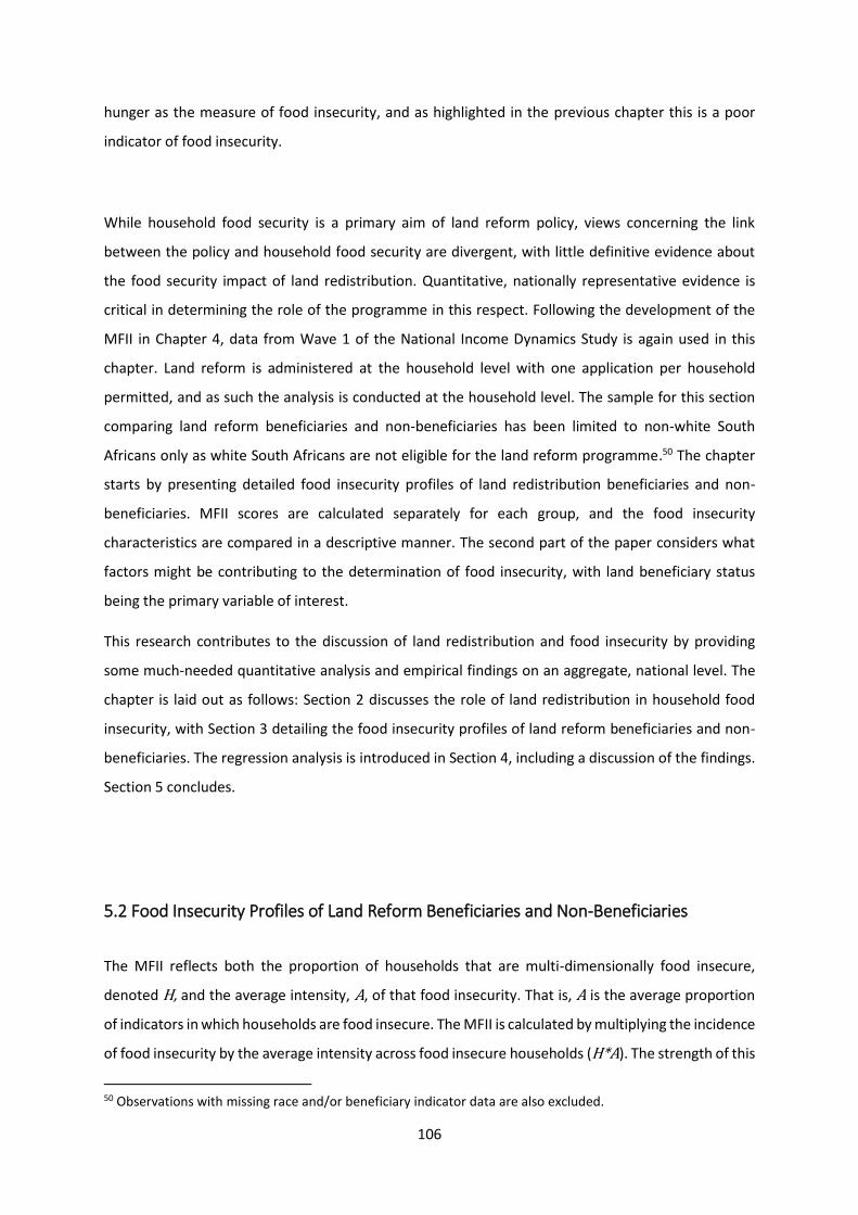
106
hunger as the measure of food insecurity, and as highlighted in the previous chapter this is a poor
indicator of food insecurity.
While household food security is a primary aim of land reform policy, views concerning the link
between the policy and household food security are divergent, with little definitive evidence about
the food security impact of land redistribution. Quantitative, nationally representative evidence is
critical in determining the role of the programme in this respect. Following the development of the
MFII in Chapter 4, data from Wave 1 of the National Income Dynamics Study is again used in this
chapter. Land reform is administered at the household level with one application per household
permitted, and as such the analysis is conducted at the household level. The sample for this section
comparing land reform beneficiaries and non-beneficiaries has been limited to non-white South
Africans only as white South Africans are not eligible for the land reform programme.50 The chapter
starts by presenting detailed food insecurity profiles of land redistribution beneficiaries and non-
beneficiaries. MFII scores are calculated separately for each group, and the food insecurity
characteristics are compared in a descriptive manner. The second part of the paper considers what
factors might be contributing to the determination of food insecurity, with land beneficiary status
being the primary variable of interest.
This research contributes to the discussion of land redistribution and food insecurity by providing
some much-needed quantitative analysis and empirical findings on an aggregate, national level. The
chapter is laid out as follows: Section 2 discusses the role of land redistribution in household food
insecurity, with Section 3 detailing the food insecurity profiles of land reform beneficiaries and non-
beneficiaries. The regression analysis is introduced in Section 4, including a discussion of the findings.
Section 5 concludes.
5.2 Food Insecurity Profiles of Land Reform Beneficiaries and Non-Beneficiaries
The MFII reflects both the proportion of households that are multi-dimensionally food insecure,
denoted H, and the average intensity, A, of that food insecurity. That is, A is the average proportion
of indicators in which households are food insecure. The MFII is calculated by multiplying the incidence
of food insecurity by the average intensity across food insecure households (H*A). The strength of this
50 Observations with missing race and/or beneficiary indicator data are also excluded.
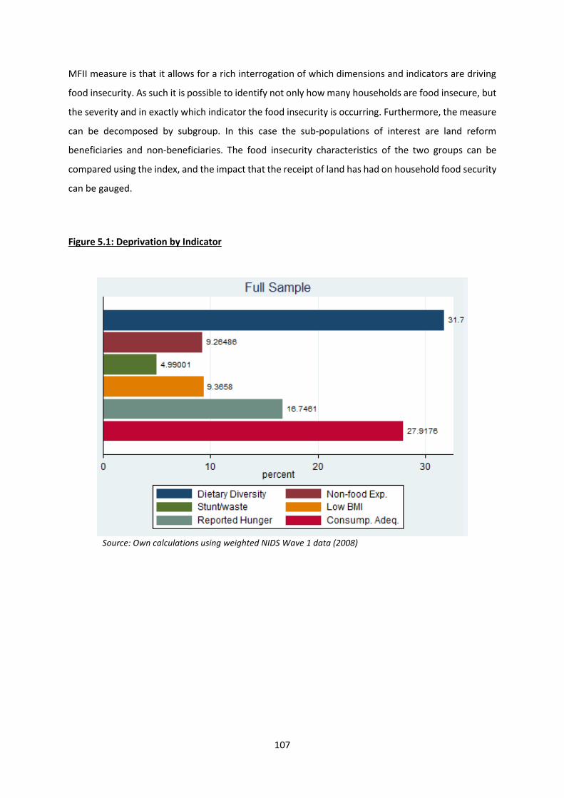
107
MFII measure is that it allows for a rich interrogation of which dimensions and indicators are driving
food insecurity. As such it is possible to identify not only how many households are food insecure, but
the severity and in exactly which indicator the food insecurity is occurring. Furthermore, the measure
can be decomposed by subgroup. In this case the sub-populations of interest are land reform
beneficiaries and non-beneficiaries. The food insecurity characteristics of the two groups can be
compared using the index, and the impact that the receipt of land has had on household food security
can be gauged.
Figure 5.1: Deprivation by Indicator
Source: Own calculations using weighted NIDS Wave 1 data (2008)
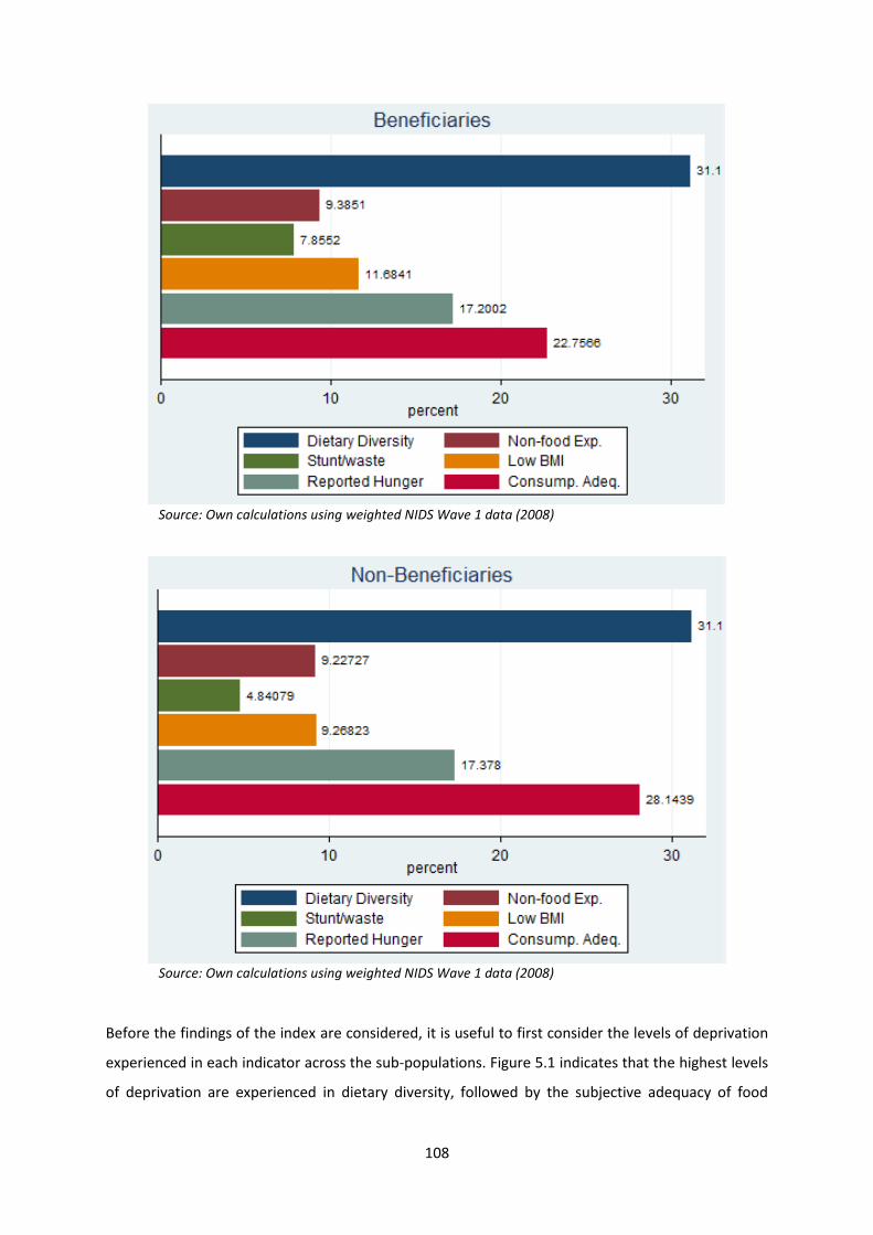
108
Source: Own calculations using weighted NIDS Wave 1 data (2008)
Source: Own calculations using weighted NIDS Wave 1 data (2008)
Before the findings of the index are considered, it is useful to first consider the levels of deprivation
experienced in each indicator across the sub-populations. Figure 5.1 indicates that the highest levels
of deprivation are experienced in dietary diversity, followed by the subjective adequacy of food
109
consumption across the full sample, beneficiaries, and non-beneficiaries. The third indicator with the
highest level of deprivation across the three groups is self-reported hunger. Dietary diversity is an
objective measure while consumption adequacy and hunger are subjective measures. This is a
noteworthy distinction as it highlights the importance of incorporating self-perceived indicators as
well as objective measures when considering food insecurity. The difference in the deprivation levels
between beneficiaries and non-beneficiaries is that stunting and wasting and low BMI are more
prevalent for beneficiaries than for non-beneficiaries. Non-beneficiaries are more deprived in self-
reported food consumption adequacy than beneficiaries. Overall the deprivation profiles of land
reform beneficiaries and non-beneficiaries are largely consistent.
Table 5.1: Multidimensional Food Insecurity Measures
Sample Incidence (H) Intensity (A) MFII % Vulnerable % Severe
Full 0.418 0.433 0.181 30.00 19.33
Beneficiaries 0.428 0.443 0.190 33.89 20.64
Non-beneficiaries 0.428 0.436 0.186 29.62 20.40
Source: Own calculations using weighted NIDS Wave 1 data (2008). 10% of the full sample are missing
information on beneficiary status and are thus not included in either the beneficiary or non-beneficiary sub-
populations. The full sample is therefore more than just the sum of the beneficiaries and non-beneficiaries, and
It is possible then that the MFII, Intensity, and Incidence for the full sample are lower than for these two sub-
populations.
Table 5.1 provides a summary of multidimensional food insecurity for all black households in South
Africa, as well as for land reform beneficiaries and for non-beneficiaries. The first column indicates the
multidimensional headcount ratio (H). This is the fraction of the sub-population that is classified as
food insecure according to the cut-offs defined. The MFII approach indicates that 41.8% of black
households in South Africa are food insecure. This figure, while considerably high, is in line with those
from alternative measurements found in the literature.51 The headcount is higher for land reform
beneficiary households at 42.8%, and the same for non-beneficiary households.52
The second column shows the average intensity of food insecurity among the food insecure (A). This
is a measure of the number of indicators in which the MFII food insecure are deprived. There are slight
differences between the intensity of the full sample, beneficiary, and non-beneficiary households at
43.3%, 44.6%, and 43.6% respectively. All the groups are deprived in 2 to 3 of the indicators.
51 See Rose & Charlton, 2002; Labadarios, Steyn & Nel, 2011. 52 Before rounding the headcount for beneficiaries is 0.4282 and 0.4277 for non-beneficiaries
110
The MFII score is found in column 3. This measure is sensitive to both the proportion of households
that are food insecure, as well as the number of indicators in which the food insecure households are
deprived. In this way the MFII accounts for both the depth and the severity of food insecurity. The
MFII for black households in South African is 0.181, and for land reform beneficiary households this is
higher at 0.190, and 0.186 for non-beneficiary households. The headcount and the average intensity
are both highest for beneficiary households, so it is expected that the MFII would be highest for this
group.
One of the capabilities of the MFII is to extend the analysis to identifying those who are vulnerable to
food insecurity. It is common in the multidimensional poverty literature to define the vulnerable as
those who are deprived in 20% to just below 33.3% of weighted indicators (Finn et al, 2013).
Considering that the cut-off for food insecurity classification is 33.3%, these are individuals who are
close to the cut-off but are not classified as food insecure. Following this convention, column 4
indicates that 30% of black households are vulnerable to food insecurity, with 33.89% of beneficiary
households and 26.62% of non-beneficiary households being vulnerable. When added to the
headcount, this indicates that more than 70% of black South African households are either food
insecure or vulnerable to food insecurity.
The MFII also allows for the identification of those suffering from severe food insecurity. Severe food
insecurity is defined as being deprived in at least half of the weighted indicators. Column 5 reveals
that nearly 20% of black households are severely food insecure. Land beneficiary and non-beneficiary
households experience similar incidence of severe food insecurity at 20.64% and 20.40% respectively.
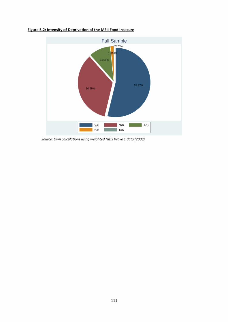
111
Figure 5.2: Intensity of Deprivation of the MFII Food Insecure
Source: Own calculations using weighted NIDS Wave 1 data (2008)
53.77%34.69%
9.911%
1.338%
.2875%
2/6 3/6 4/6
5/6 6/6
Full Sample
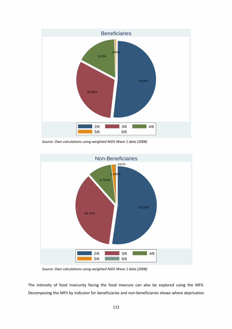
112
Source: Own calculations using weighted NIDS Wave 1 data (2008)
Source: Own calculations using weighted NIDS Wave 1 data (2008)
The intensity of food insecurity facing the food insecure can also be explored using the MFII.
Decomposing the MFII by indicator for beneficiaries and non-beneficiaries shows where deprivation
51.8%
30.99%
16.8%
.419%
2/6 3/6 4/6
5/6 6/6
Beneficiaries
52.32%
36.15%
9.752%
1.436%
.341%
2/6 3/6 4/6
5/6 6/6
Non-Beneficiaries
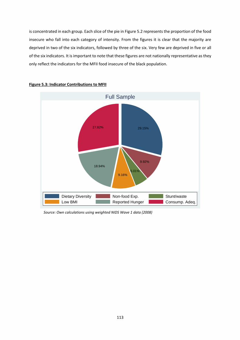
113
is concentrated in each group. Each slice of the pie in Figure 5.2 represents the proportion of the food
insecure who fall into each category of intensity. From the figures it is clear that the majority are
deprived in two of the six indicators, followed by three of the six. Very few are deprived in five or all
of the six indicators. It is important to note that these figures are not nationally representative as they
only reflect the indicators for the MFII food insecure of the black population.
Figure 5.3: Indicator Contributions to MFII
Source: Own calculations using weighted NIDS Wave 1 data (2008)
29.15%
9.92%
5.01%
9.16%
18.94%
27.82%
Dietary Diversity Non-food Exp. Stunt/waste
Low BMI Reported Hunger Consump. Adeq.
Full Sample
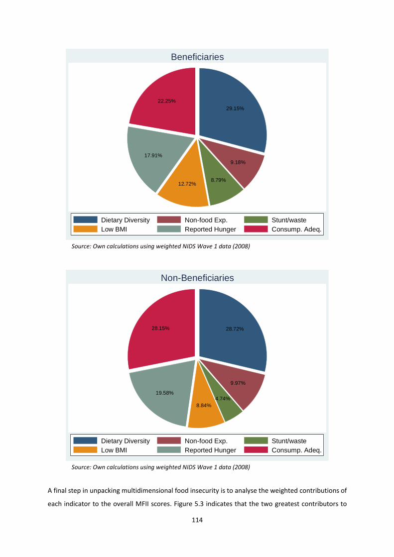
114
Source: Own calculations using weighted NIDS Wave 1 data (2008)
Source: Own calculations using weighted NIDS Wave 1 data (2008)
A final step in unpacking multidimensional food insecurity is to analyse the weighted contributions of
each indicator to the overall MFII scores. Figure 5.3 indicates that the two greatest contributors to
29.15%
9.18%
8.79%12.72%
17.91%
22.25%
Dietary Diversity Non-food Exp. Stunt/waste
Low BMI Reported Hunger Consump. Adeq.
Beneficiaries
28.72%
9.97%
4.74%
8.84%
19.58%
28.15%
Dietary Diversity Non-food Exp. Stunt/waste
Low BMI Reported Hunger Consump. Adeq.
Non-Beneficiaries
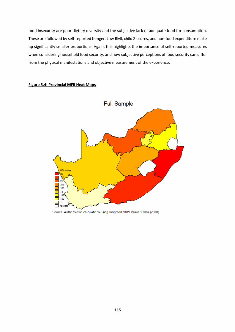
115
food insecurity are poor dietary diversity and the subjective lack of adequate food for consumption.
These are followed by self-reported hunger. Low BMI, child Z-scores, and non-food expenditure make
up significantly smaller proportions. Again, this highlights the importance of self-reported measures
when considering household food security, and how subjective perceptions of food security can differ
from the physical manifestations and objective measurement of the experience.
Figure 5.4: Provincial MFII Heat Maps
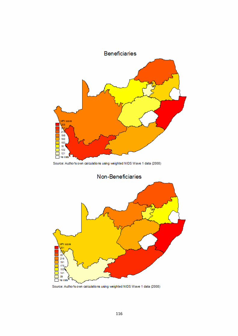
116
117
The provincial breakdown of beneficiary and non-beneficiary household food insecurity can also be
examined using the MFII. Figure 5.4 presents heat maps showing the MFII scores of each province, by
beneficiary status. KwaZulu-Natal suffers the highest levels of multidimensional food insecurity,
regardless of beneficiary status. This is followed by the Western Cape for land reform beneficiaries,
and Limpopo for non-beneficiaries. It is interesting that beneficiaries in the Western Cape suffer the
second highest levels of food insecurity, as this province generally suffers the least food insecurity for
the full sample, as well as at the national level. A more detailed analysis of food insecurity in the
Western Cape can be conducted using the MFII to identify which of the indicators are the main drivers
of food insecurity amongst land reform beneficiaries.
5.3 Factors Determining Food Insecurity Status
From the profiles presented there are few meaningful differences in the food insecurity status of land
redistribution beneficiary and non-beneficiary households. Generally beneficiary households have a
higher MFII score than non-beneficiaries, at 0.190 and 0.186 respectively, indicating that they are
more multidimensionally food insecure. This is driven by the higher intensity of the food insecurity
experienced by beneficiaries, while the incidence is the same for both groups. Poor dietary diversity
and subjective inadequacy of food consumption are the greatest contributors to food insecurity for
both beneficiary and non-beneficiary households.
Following the descriptive picture of the food insecurity status of beneficiary and non-beneficiary
households, a natural question that arises is how to analyse the causes of multidimensional food
insecurity. Micro regressions, focussing on the individual or household as the unit of analysis, present
a useful tool for looking at the determinants of poverty and other Alkire-Foster poverty measures,
including the MFII (Alkire, Foster, Seth, Santos, Roche & Ballon, 2015). An intuitive way is to model the
probability of a household becoming multidimensionally food insecure, as suggested by Alkire, Foster,
Seth, Santos, Roche & Ballon (2015).53 From a policy perspective, this is more useful than simply
measuring food insecurity, and allows for an understanding of how policy can translate into improved
outcomes. The simplest model is a linear probability model, with the dependent variable being a
binary variable indicating the food insecurity status of the household (Alkire et al, 2015). In this section
this suggested approach is followed and the probability that a household is 1) food insecure, and 2)
severely food insecure is assessed, based on several demographic and socioeconomic characteristics
53 Multidimensionally poor in their case
118
of the household. By using a regression approach where household characteristics are controlled for,
the role played by land redistribution in the food insecurity status of households can be disentangled.
Before continuing there is an important difference to be noted between the food insecurity profiles
presented in Section 2 and this section of the analysis. The previous section considered land
redistribution beneficiaries and non-beneficiaries as two separate sub-populations. As such, for
comparative purposes, MFII scores and the resultant descriptive statistics are generated separately
for the two groups. In this second part of the analysis the sample of all black households is considered
as a whole, and the beneficiaries and non-beneficiaries are not separated as distinct sub-populations.
This is because the analysis considers the probability of any black household in South Africa being food
insecure based on a set of characteristics, with beneficiary status being a key explanatory variable. As
such the dependent variable is based on the MFII score as calculated for the full sample of black
households.
The model presented here draws heavily on the motivation and discussion outlined for the welfare
regression in Chapter 3, and as such this will not be repeated. The control variables are largely the
same, with the major difference being the dependent variable. Where Chapter 3 utilised a general
measure of household welfare, this model uses the MFII as a measure of household food insecurity
status. Two separate linear probability models are estimated: the first considering the probability of a
household being multidimensionally food insecure, and the second considering the probability of a
household being severely multidimensionally food insecure. According to the specification outlined in
Chapter 4, a food insecure household is one that is deprived in two or more of the six indicators, while
a severely food insecure household is deprived in at least three of the six indicators. As such, being
classified as food insecure includes those who are severely so.
The key explanatory variable is an indicator of whether the household has received a land grant
through the redistribution programme. An indicator of whether the household is involved in any
agricultural activity is also included, for the same reasons as discussed in Chapter 3, namely the low
correlation between beneficiary status and agricultural activity at 0.04.54 An interaction term of land
reform beneficiary status and agricultural activity is also included. Unfortunately access to land cannot
be controlled for in this model as it is in Chapter 3 due to data limitations discussed below. In addition
to these three primary controls, income and demographic drivers, household structural
characteristics, and geographic variables are considered for their role in explaining food insecurity,
namely: province; rural or urban location; a measure of the assets owned by the household – car and
54 Own calculation using NIDS Wave 1 data
119
phone; access to services in the form of grid electricity and piped water; an indicator for whether the
household has received a housing grant; an indicator for whether someone in the household receives
a government grant; the proportion of adults in the household; the proportion of working-age adults
who are employed in the household; and the gender, age and education level (no schooling, primary,
secondary without matric, matric, or tertiary) of the household head. A measure of household income
or expenditure is not included directly as a control variable. If it is believed that receiving land
increases the income and/or expenditure of a household, and that this increase reduces food
insecurity, it may be argued that the coefficient on the land beneficiary dummy is limited to picking
up the effect of receiving land over and above its effect on income and/or expenditure regressors
(Valente, 2009). Rather, socio-economic status is inferred from variables including asset ownership,
grant receipt, access to services, employment levels, and household head characteristics.
While the model presented here and that in Chapter 3 are very similar and both use NIDS data, this
chapter uses Wave 1 data from 2008, which was used to create the MFII, and not Wave 4 data from
2014 and 2015 that was used in Chapter 3. The weighting issues encountered when using Wave 4 are
thus not a problem, and these results are weighted to be nationally representative.
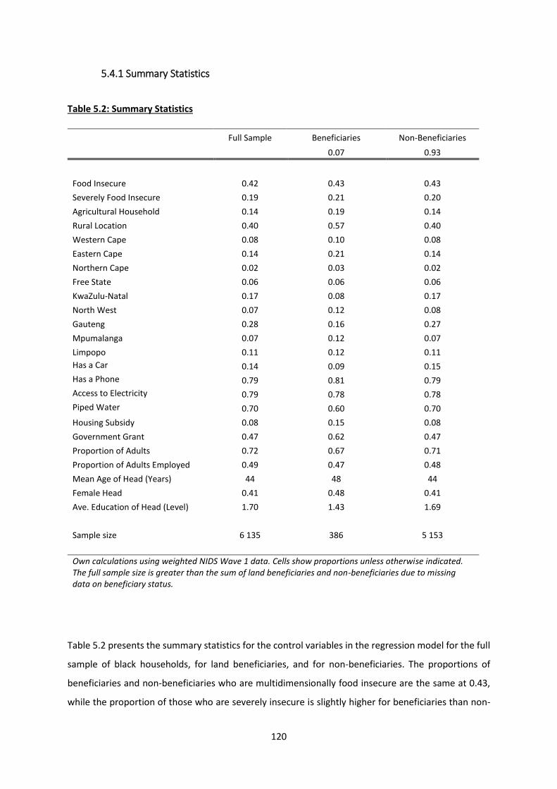
120
5.4.1 Summary Statistics
Table 5.2: Summary Statistics
Full Sample Beneficiaries Non-Beneficiaries
0.07 0.93
Food Insecure 0.42 0.43 0.43
Severely Food Insecure 0.19 0.21 0.20
Agricultural Household 0.14 0.19 0.14
Rural Location 0.40 0.57 0.40
Western Cape 0.08 0.10 0.08
Eastern Cape 0.14 0.21 0.14
Northern Cape 0.02 0.03 0.02
Free State 0.06 0.06 0.06
KwaZulu-Natal 0.17 0.08 0.17
North West 0.07 0.12 0.08
Gauteng 0.28 0.16 0.27
Mpumalanga 0.07 0.12 0.07
Limpopo 0.11 0.12 0.11
Has a Car 0.14 0.09 0.15
Has a Phone 0.79 0.81 0.79
Access to Electricity 0.79 0.78 0.78
Piped Water 0.70 0.60 0.70
Housing Subsidy 0.08 0.15 0.08
Government Grant 0.47 0.62 0.47
Proportion of Adults 0.72 0.67 0.71
Proportion of Adults Employed 0.49 0.47 0.48
Mean Age of Head (Years) 44 48 44
Female Head 0.41 0.48 0.41
Ave. Education of Head (Level) 1.70 1.43 1.69
Sample size 6 135 386 5 153
Own calculations using weighted NIDS Wave 1 data. Cells show proportions unless otherwise indicated. The full sample size is greater than the sum of land beneficiaries and non-beneficiaries due to missing data on beneficiary status.
Table 5.2 presents the summary statistics for the control variables in the regression model for the full
sample of black households, for land beneficiaries, and for non-beneficiaries. The proportions of
beneficiaries and non-beneficiaries who are multidimensionally food insecure are the same at 0.43,
while the proportion of those who are severely insecure is slightly higher for beneficiaries than non-
121
beneficiaries at 0.21 and 0.20 respectively. This reflects the indication from the food insecurity profiles
that while the headcounts of the food insecure are the same for beneficiaries and non-beneficiaries,
the intensity is greater for beneficiaries. The proportion of beneficiary households that are involved
in agriculture is considerably greater than non-beneficiaries at 0.19 and 0.14 respectively. While this
is an encouraging association, the figures are still generally low given that the purpose of land
redistribution is to increase agricultural production. This finding is however consistent with that
suggested in Chapter 3, as well as the additional analysis mentioned there using the HSRC data set.
More than half of beneficiary households, 0.57, are located in rural areas while 0.40 of non-
beneficiaries live in rural areas. The greatest proportion of beneficiaries reside in Gauteng, 0.16, while
the smallest proportion live in the Northern Cape, 0.03. The relative locations of non-beneficiaries is
the same, and this reflects the relative distribution of households in the full sample. In terms of asset
ownership fewer beneficiaries own a car than non-beneficiaries at 0.09 and 0.15, while the two groups
both enjoy high proportions of phone ownership (landline and/or cell phone) at 0.81 for beneficiaries
and 0.79 for non-beneficiaries. Access to electricity is the same for the two groups at 0.78. The
proportion of beneficiaries having piped water in the dwelling is somewhat smaller than that of non-
beneficiaries at 0.60 and 0.70 respectively. A greater proportion of beneficiary households receive
housing subsidies and social grants, at 0.15 and 0.62 respectively, than non-beneficiary households at
0.08 and 0.47. Beneficiary households comprise a slightly smaller proportion of adults than non-
beneficiary households at 0.67 and 0.71, while the proportion of adults who are employed in
beneficiary households, 0.47, is very similar to that of non-beneficiary households, 0.48. There are
not any notable differences in the characteristics of the household heads of beneficiary and non-
beneficiary households, with beneficiary heads being slightly older at 48 versus 44, and both groups
having an average of primary school education. A somewhat greater proportion of beneficiary
households are headed by women, at 0.48 and 0.41 respectively.
The most noteworthy revelation from the summary statistics is the very low proportion of land
beneficiaries involved in household agricultural activities, and the somewhat small proportion of
beneficiary households living in rural areas. The indication is that only just over half of land reform
beneficiaries are living in rural areas, and that only 19% of all beneficiary households are involved in
farming activities. This is concerning as land redistribution is focused only on rural areas, and a primary
aim of land redistribution policy is to increase the farming productivity of households. These findings
do however reflect those found in Chapter 3 using NIDS, as well as the similar study using the HSRC
data. This begs the question again of what has happened to the land received through the programme
if it is not being used for productive purposes. As discussed in Chapter 3, case studies indicate that
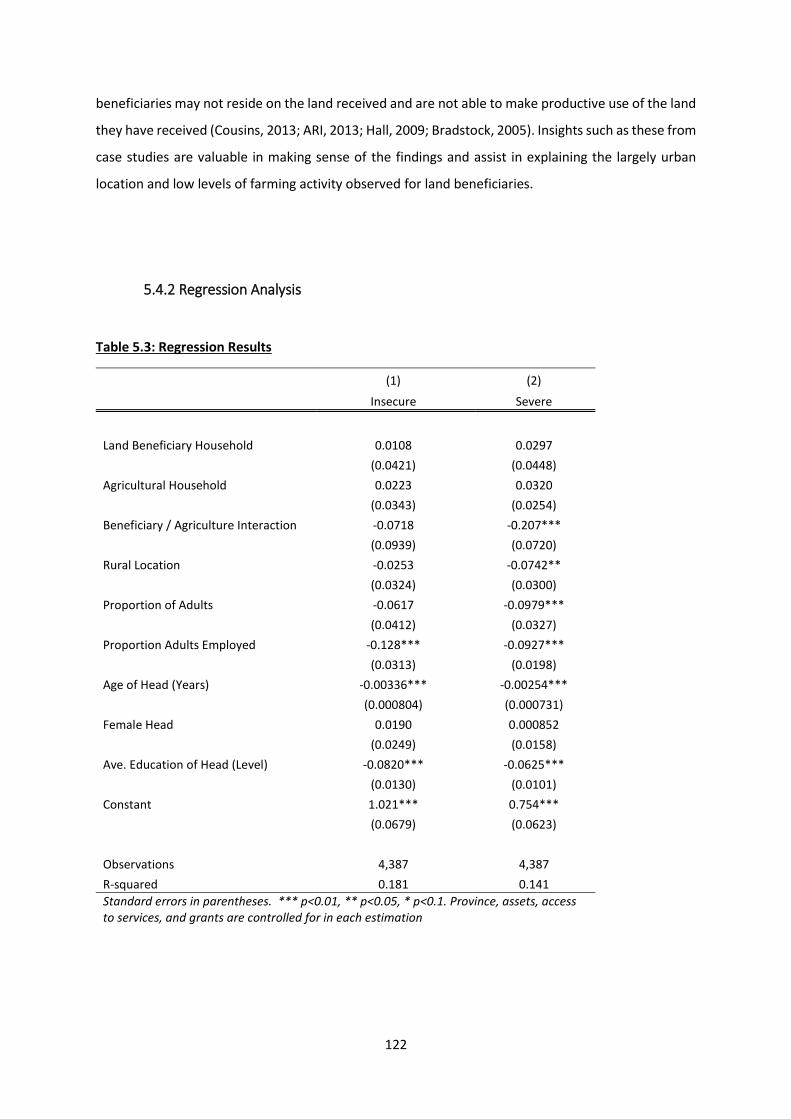
122
beneficiaries may not reside on the land received and are not able to make productive use of the land
they have received (Cousins, 2013; ARI, 2013; Hall, 2009; Bradstock, 2005). Insights such as these from
case studies are valuable in making sense of the findings and assist in explaining the largely urban
location and low levels of farming activity observed for land beneficiaries.
5.4.2 Regression Analysis
Table 5.3: Regression Results
(1) (2)
Insecure Severe
Land Beneficiary Household 0.0108 0.0297
(0.0421) (0.0448)
Agricultural Household 0.0223 0.0320
(0.0343) (0.0254)
Beneficiary / Agriculture Interaction -0.0718 -0.207***
(0.0939) (0.0720)
Rural Location -0.0253 -0.0742**
(0.0324) (0.0300)
Proportion of Adults -0.0617 -0.0979***
(0.0412) (0.0327)
Proportion Adults Employed -0.128*** -0.0927***
(0.0313) (0.0198)
Age of Head (Years) -0.00336*** -0.00254***
(0.000804) (0.000731)
Female Head 0.0190 0.000852
(0.0249) (0.0158)
Ave. Education of Head (Level) -0.0820*** -0.0625***
(0.0130) (0.0101)
Constant 1.021*** 0.754***
(0.0679) (0.0623)
Observations 4,387 4,387
R-squared 0.181 0.141
Standard errors in parentheses. *** p<0.01, ** p<0.05, * p<0.1. Province, assets, access to services, and grants are controlled for in each estimation
123
Table 5.3 presents the results of the linear probability estimates for both the food insecurity and the
severe food insecurity regressions. Logit marginal effects are presented in Appendix A5.1, and confirm
these findings. Specification 1 regresses the probability of a household being multidimensionally food
insecure on various controls, including the key indicators for beneficiary status and agricultural
activity, and the interaction of these two. None of these primary explanatory variables has a significant
bearing on the probability of a household being food insecure. The factors that are significant are the
proportion of adults who are employed in the household, and the age and education of the household
head, all of which have a negative relationship with the probability of a household being food insecure.
Specification 2 regresses the probability of a household being severely multidimensionally food
insecure on the same set of control variables. Both the land beneficiary status and agricultural activity
indicators are not significant factors, while the interaction of the two has a significantly negative
bearing on the probability of a household being severely food insecure. While there is no overall effect
of either beneficiary status or agricultural activity alone, the two are jointly significant, suggesting that
only land redistribution beneficiaries who are agriculturally active have a decreased probability of
being severely food insecure. The rural location, proportion of adults in the households, proportion of
adults, and the age and education level of the household head also have a significant effect of reducing
the probability of a household being severely food insecure.
The lack of a significant impact of land received through the land redistribution programme seems to
suggest that this policy is most likely not having the intended impact of improving household food
insecurity. This reflects the findings in Chapter 3 that land redistribution is not a straightforward
solution to improving household welfare in general. While some recipients may indeed be reaping the
benefits of land receipt on a limited and ad hoc basis, the impact and benefits do not appear to be
systematic or widespread. The insignificance of household agricultural activity in terms of improving
food insecurity causes additional concerns, as subsistence farming is the primary means through
which land redistribution is assumed to translate into improved food insecurity outcomes. What is
encouraging however is the significance of the interaction of beneficiary status and agricultural
activity. The suggestion is that when beneficiary households are indeed engaged in farming activity,
the probability of being severely food insecure is significantly reduced. This is an important finding for
the efficacy of land redistribution policy, while the indication is that if the receipt of land does not
translate into increased production, the benefits of improved food insecurity cannot be realised. This
highlights the problematic nature of the assumption that access to land will translate into improved
household food security, without considering the essential link of the land being used productively. A
glaring challenge that remains however is the low proportion of beneficiary households that are
actively engaging in farming activity. More targeted selection of land redistribution beneficiaries

124
towards those already engaged in small scale farming activities in rural areas may be an important
step in improving the efficacy of land redistribution.
While there is no direct measure of household income in the analysis the significance of a number of
the proxies for socio-economic status, household head characteristics and employment levels, speaks
to the importance of income in determining household food insecurity. This is important in the face
of rising food prices currently experienced in South Africa. The South African Reserve Bank has stated
that local food price inflation is expected to rise to 11.6% in the fourth quarter of 2016.55 The dramatic
increase is attributed to various factors, including increasing prices of electricity and water, persistent
drought, and the weak Rand. The significance of income proxy measures together with increasing food
prices has an impact on almost all the six indicators of multidimensional food insecurity. This is felt
most acutely by the poor who are forced to substitute lower quality food and/or increase the
household indebtedness to meet their food requirements. Their consumption of less diverse and
nutritionally inferior food has various impacts on child growth and adult health. These concerns link
back to the discussion in the food insecurity literature indicating that subsistence agriculture must
translate into increased income to have a meaningful impact on household food insecurity.
5.5 Conclusion
A fundamental premise of the land redistribution programme is that the provision of land to the poor
will realise greater food security through the productive utilisation of the land resource (Department
of Land Affairs, 2003). However, as highlighted in Chapter 3, the premise of access to land translating
into increased agricultural production is assumed rather than verified. The suggestion from that
chapter is that land redistribution is likely not a clear-cut solution to issues of social welfare and rural
development. No systematic, positive impact of the policy was shown, and while there are some
benefits to be derived, the nuances for effective land redistribution are complex and a clear picture
has yet to be defined. The findings from Chapter 3 did not provide conclusive indications about the
role that land redistribution plays, or can play, in improving household outcomes. This section sought
to further explore this in considering the food security impact of land receipt. Using the new MFII as
opposed to one of the single proxy measures commonly used, ensures that the complexity of what it
55 https://www.resbank.co.za/Lists/News%20and%20Publications/Attachments/7223/MPC%20Statement%2017%20March%202016%20.pdf
125
means to be food insecure is captured, rather than some related, yet limited, concept such as hunger
or dietary diversity. In light of this distinction, this is the first empirical research exploring the links
between land redistribution and true household food insecurity in South Africa. This study contributes
both to the land redistribution literature as a quantitative analysis of the household outcomes, as well
as the food insecurity literature as an application of a new measure. While the ideal comparative
analysis would be a pre-post design, where the food insecurity status of beneficiaries and non-
beneficiaries could be contrasted definitively, the evidence presented here is useful in considering the
multidimensional food insecurity status of the two groups.
The results provide a detailed comparative picture of the state of food insecurity of land reform
beneficiary and non-beneficiary households, as well as the factors that play an important role in
influencing food insecurity status. In terms of comparing the food insecurity profiles of land
beneficiaries and non-beneficiaries there is little difference in the numerous aspects of their food
insecurity. In general land redistribution beneficiaries have a higher MFII score than non-beneficiaries,
and suffer greater severity in food insecurity. The overall indication from the descriptive application is
that those who have received land through the land reform programme do not appear any better off
in terms of food insecurity than those who have not, and possibly suffer even more. It must be noted
however that the design of this analysis does not discount the possibility that land redistribution has
improved beneficiary household food security from some even lower base, and brought it more in line
with the food security levels of non-beneficiaries.
This seemingly limited impact of land redistribution is also apparent when considering the factors that
have a bearing on food insecurity status through regression analysis. Individuals living in households
that have received land are not significantly more or less likely to be food insecure, or severely
insecure, than those in households that have not received land. The same can be said of households
engaging in agricultural activity, in that subsistence farming does not seem to have a significant
bearing on food insecurity status. Importantly however, the significant interaction of beneficiary
status and agricultural activity is an encouraging finding for land reform policy in general. The
indication is that when the land that has been received is indeed being used as intended for
agricultural production, the anticipated outcomes may be realised. The concern about redistributed
land not being used productively, as suggested by the descriptive statistics, remains a substantial
obstacle. As noted, many beneficiaries are not actively engaged with farming projects taking place on
the land which they have received (Cousins, 2013; ARI, 2013; Hall, 2009; Bradstock; 2005). This is a
difficulty that speaks to the implementation of land redistribution more generally. There is a clear
disjuncture between the policy aims of increased productivity and what seems to be happening in
practice, which is something that should be seriously considered in improving the outcomes of the
126
policy. While this evidence is anecdotal rather than empirical, it does provide important insights into
why such limited results from land redistribution might be observed. Further studies are required that
explore in depth what has happened to land that has been redistributed, and why some beneficiary
households are involved in farming activities and others are not. This line of research is key if land
reform policy is to be pursued in any meaningful way.
127
Chapter 6: Exploring the Limits to Social
Preferences for Redistribution
6.1. Introduction
Chapters 3, 4, and 5 of this thesis focus on the economic aspects of land in terms of the relationship
between land redistribution and household welfare and food insecurity. The findings are not overly
persuasive about the positive role that redistributed land plays in the economic wellbeing of
beneficiaries. However, land remains an emotive and highly-charged issue in South Africa as it played
a key role in entrenching racial segregation during apartheid, and has since become an important
symbol of restitution and recognition of the atrocities of the past. As such, in addition to its productive
and economic value, land is intimately linked to ideas of fairness and distributive justice. Notions of
inequality, distributive justice, and fairness are therefore prominent in the context of land reform
policy in South Africa. In particular, land restitution policy is guided by the principals of fairness and
justice, with the purpose of compensating victims of racially-based land dispossession (DLA, 1997).
Following the findings in the previous chapters the focus of this chapter shifts away from the purely
economic aspect of land to one of a more social nature. The consideration turns to the broader notions
of inequality, fairness, and preferences for redistribution, concepts which are closely linked to land in
South Africa.
South Africa is a unique and interesting setting in which to explore issues of inequality, as well as
fairness and social preferences for redistribution. The historical context of apartheid and the
consequent policies aimed at directly addressing the resultant inequality have entrenched the
concepts of fairness, inequality, and redistribution in the consciousness of most South Africans. The
prominence of these issues and concepts in the social makeup of the country make it an ideal and
interesting context for this research. South Africa is one of the most unequal countries in the world,
with a Gini Index coefficient of 0.63 (World Bank, 2013). The demand for redistribution is however
puzzling, in that while the country has one of the highest levels of inequality in the world the demand
for redistribution is only average, and in fact lower than in other non-OECD countries (Pellicer, Piraino
& Wegner, 2014). Indications are that while South Africans are generally disappointed by small
economic returns since democratisation, they generally demand jobs rather than redistribution
through social welfare (Pellicer, Piraino & Wegner, 2014). Indications from the World Values Survey
(2013) are that South Africans tend to believe that hard work pays off in the long run rather than
128
success being a matter of luck and connections. The tendency is toward a belief that larger income
differences are incentives for individual effort, rather than that they should be made more equal.
Perceptions are roughly equal about whether people should take more responsibility to provide for
themselves or that government should take this responsibility.56
Notions of inequality, fairness, and preferences for redistribution are not easily measured or isolated
for quantification, and survey data methods as applied in the previous chapters would be inadequate.
Behavioural experiments, however, provide a useful approach for studying and understanding social
preferences and views on fairness and redistribution. Experimental economics has gathered
unambiguous evidence that systematically refutes the self-interest hypothesis, and indicates that
people are strongly motivated by fairness considerations (Fehr & Schmidt, 2001). As such there are a
number of accepted truths regarding social preferences for fairness and the willingness to
redistribute. People generally have a preference for fairness, and they are willing to suffer some
monetary loss to ensure a fairer outcome. In addition, inequality acceptance is higher when the source
of the inequality is deemed to be fair. Ideas about fairness are also often interlinked with views about
what an acceptable level of inequality is (Alesina & Giuliano, 2009). Using a behavioural experiment
this paper delves deeper into these issues, and investigates the limits to the willingness to redistribute.
More specifically, the experiment explores the impact of two factors on the willingness to redistribute:
the personal cost involved, and the size of the initial inequality.
In seeking to understand how people make choices most models associate choices with the utility
gained from making those choices. While this is unobservable, under certain conditions such as those
in a behavioural experiment, something can be inferred about peoples’ preferences from the choices
they make. The interpretation of the findings from this experiment are guided by the Cappelen et al
(2007; 2013) motivation function, which trades off a desire for fairness with self-interest motivations.
The impact that personal cost and initial inequality have on the choice to redistribute is interpreted
and discussed with reference to this utility model. The core hypothesis is that the greater the personal
cost involved the lower the willingness to redistribute, as the motivation for self-interest increases
relative to fairness considerations. The effect of selfish considerations on the willingness to
redistribute has scarcely been studied directly. This research design introduces a monetary cost to the
decision to redistribute, and measures how, as a measure of self-interest, this personal cost affects
inequality acceptance. The hypothesis is that the greater the personal cost, the lower the willingness
to redistribute. Regarding the size of the initial income inequality the hypothesis is that higher levels
of inequality are viewed as more unfair than lower levels of inequality. As such, the greater the initial
56 Own calculations using the World Values Survey data for South Africa, 2013. www.worldvaluessurvey.org
129
inequality the greater the subsequent willingness to redistribute for a fair outcome. Regarding the
cost involved, the hypothesis is that the larger the initial inequality the higher the cost people are
willing to bear to effect a fair outcome.
The effects of cost and inequality are further contextualised in terms of the source of income
inequality - luck or merit. Societal preferences for redistribution and support for redistributive policies
appear to reflect differences in social perceptions regarding the fairness of market outcomes and the
underlying sources of inequality. For instance, Americans are more likely to believe that wealth and
success are the outcome of hard work and individual effort, whereas Europeans believe that luck,
corruption, and connections play a greater role (Alesina & Angeletos, 2005). Theories of distributive
justice provide guidance as to what a fair distribution of income in a society might be, with these
principals guiding what is deemed fair and unfair. People often feel that there is a difference between
wealth accumulated through pure luck, and wealth earned through hard work. In line with the liberal
egalitarian view of distributive justice, it has been shown empirically that individuals have a sense that
one is more entitled to retain income earned from effort than income acquired by luck (Alesina &
Giuliano, 2009). In this sense, income inequality as a result of personal effort is considered to be fairer
than income inequality arising as a result of luck. While definitions of luck and effort can differ greatly,
many people consider the distinction relevant to their preferences for inequality and redistribution,
and inequality acceptance by participants is generally found to be higher when the source of the
income inequality is due to effort rather than random luck (Alesina & Giuliano, 2009).
By varying the levels of personal cost and initial inequality this research provides innovative insights
into social preferences for redistribution, and new causal evidence on how self-interest and fairness
considerations shape distributive choices. The findings reveal that the level of personal cost and the
magnitude of the initial inequality matter for preferences for redistribution and fairness views, and
provide further confirmation that the source of the inequality is also a contributing factor.
In arriving at these results, the rest of the paper is laid out as follows: Section 2 offers a detailed
discussion of distributive justice. This is followed by a review of the experimental literature on fairness
in Section 3. Section 4 introduces the experiment design, and the findings and analysis are presented
in Section 5. Section 6 concludes.
130
6.2 Distributive Justice
Decisions about inequality acceptance are guided by the philosophy of distributive justice and fairness.
Distributive justice in its modern sense calls on the state to guarantee that everyone is supplied with
a certain level of material means (Fleischacker, 2005). Governments continuously make and change
laws affecting the distribution of economic benefits and burdens in their societies, with the effect that
different societies have different distributions (Lamont & Favor, 2008). Distributive justice theory
provides practical guidance for choices regarding the distribution, with numerous theories suggesting
what the fair distribution of income might be. Some of the major theories include strict egalitarianism,
libertarianism, liberal egalitarianism, choice egalitarianism, and meritocracy. Each theory offers
different indications as to what is fair in the distribution of income.
Strict egalitarians argue that people should not be held responsible in any way for their effort or talent,
and thus the fair distribution of income is an equal one where every person has the same level of
material goods and services (Lamont & Favor, 2008). This would require considerable redistributive
policies on the part of government. On the other hand, libertarians believe that people should be held
responsible for their effort and talent, and therefore a fair distribution of income is one where each
person earns according to his/her productivity. In this sense inequalities arising as a result of individual
merit are fair, and the role of government is limited to protecting individual property rights rather
than redistributive action (Lamont & Favor, 2008). Liberal egalitarians are somewhere in between,
and claim that effort is within individual control, while talent is beyond individual control (Cappelen,
Hole, Sorenson & Tungodden, 2007). Thus, it would be fair to equalise differences based on talent,
while allowing for inequalities as a result of effort. In this instance the redistributive role of
government would be limited to specific types of inequality. Choice egalitarianism holds people
responsible for their choices, but not for their luck. The motivation is that within a society individuals
should not be made to give up some of their wealth, obtained for example through great effort,
because others have made poor choices, for example by choosing not to work. In some instances then,
choice egalitarianism and liberal egalitarianism may overlap if talent is characterised as luck and effort
is determined by choice. Finally, meritocrats argue that individuals should be held responsible for all
personal characteristics, including endowments such as intelligence and social networks, as well as
virtues such as effort and self-discipline. Those who deserve to succeed do, and those who succeed
are those that deserve to.
A key function of theories of distributive justice is determining which factors people are responsible
for and which factors are beyond their control. Closely linked to this are ideas about fairness.
131
Inequality arising from individual actions and choices for which one can be held responsible are
considered fairer than inequalities arising from random luck and factors beyond our control for which
one cannot be held responsible. There is some contention however as to what factors are truly under
our control and which are not. For example, are effort and self-discipline virtues as a result of luck at
birth, or are they individual choices for which one is responsible? Generally, luck and innate abilities
are considered factors beyond our control, while effort and choice are self-determined. The
relationship between fairness and personal responsibility is what defines a fairness ideal. An
individual’s fairness ideal captures what factors or attributes he/she believes people are responsible
for, and thus what the unique, fair distribution is in any given situation (Cappelen et al, 2007).
Considering that income inequality can be the result of differences in factors within and beyond one’s
control, and that people differ in their fairness ideals, some inequalities are considered acceptable
and fair while others are not.
6.3 Experimental Literature on Fairness
According to Rawls (1971), distributive justice requires that inequalities between the lucky and the
unlucky are mitigated through redistribution. Indeed, experimental evidence suggests that people do
feel that inequalities caused by factors beyond our control, such as a lottery draw, should be mitigated
to a considerable extent via redistribution (Cappelen et al, 2007; Almas, Cappelen, Sorenson &
Tungodden, 2010; Cappelen, Sorenson & Tungodden, 2010; Cappelen, Konow, Sorenson &
Tungodden, 2013). The key debate in the distributive justice literature however is what factors are
considered lucky or unlucky, and what factors an individual is responsible for.
A key factor in shaping fairness ideals is what people hold each other responsible for, with a distinction
being made between those factors that are within individual control and those that are beyond
individual control. A recent experimental study indicates that the majority of individuals do not hold
people responsible for a randomly assigned price – a factor that is beyond individual control
(Cappelen, Sorenson & Tungodden, 2010). On the other hand, there is broad support for holding
individuals responsible for their choice of working time - a factor within individual control. The
majority also held others responsible for his/her productivity. The authors deem this to be a factor
beyond individual control, and consider it interesting that it is treated differently to the randomly
assigned price. The preferred explanation is that a responsibility distinction was being made between
personal and impersonal factors, rather than between choices and circumstances. This is in line with
132
the meritocratic theory of distributive justice where people deserve the rewards from all personal
attributes. Alternatively, from the choice egalitarian perspective, differences in productivity can be
due to differences in the chosen intensity of work. This interpretation is however considered unlikely
(Cappelen, Sorenson & Tungodden, 2010).
The impact of relative economic status on individual’s notions of distributive justice has also been
explored (Barr, Burns, Miller & Shaw, 2011). In a dictator game under two treatments, one where
endowments were earned and one where they were randomly assigned, it was found that relatively
well-off individuals make allocations to others that reflect the initial endowments more when the
endowments were earned, rather than when they were randomly assigned. This was not the case
among relatively poor individuals.
In exploring the impact of a choice on attitudes to inequality Cappelen, Fest, Sorenson & Tungodden
(2014) find that the introduction of a choice significantly decreases the willingness of a spectator to
redistribute between a lucky and an unlucky participant. This result holds even when the choice has
no effect on the economic outcome. This experiment provides initial evidence that many people
consider fairness in the context of risk-taking to go beyond equalising opportunities, but it also reveals
considerable disagreement on how to fairly allocate the gains and losses from risk-taking. Generally
however, the majority favours choice egalitarianism in that most participants consider it fair to
eliminate inequalities between lucky and unlucky risk-takers.
Cappelen, Konow, Sorenson & Tungodden (2013) study fairness views about risk-taking, and
specifically whether such views are based on ex-ante opportunities or ex-post outcomes. While many
participants focus on ex ante opportunities, most favour some redistribution ex-post. A distinction is
also clear between ex post inequalities that reflect differences in luck and those that reflect
differences in choices.
Cappelen, Hole, Sorenson & Tungodden (2007) have shown that pluralism of fairness ideals is
characteristic of modern societies in that while liberal egalitarianism was the most prevalent
preferences amongst their participants, the majority of them held other fairness ideals. In studying
fairness and the development of inequality acceptance in children Almas, Cappelen, Sorenson &
Tungodden (2010) find that as children enter adolescence, they increasingly view inequalities as a
result of differences in individual achievements as fair, but differences arising as a result of luck as
unfair.
In the first nationally representative, cross-country behavioural experiment on inequality and
redistribution Almas, Cappelen and Tungodden (2016) explore differences in social preferences in
133
Norway and the United States. They find that Americans accept significantly more inequality than
Norwegians, and that this difference reflects a difference in fairness views. Further, fairness
considerations are shown to be more important for inequality acceptance than efficiency
considerations in both countries.
Considering the numerous theories of distributive justice, the question remains of what factors
individuals base their ideas of distributive justice on in the real world. This chapter explores the
interplay between selfishness, concerns for fairness, and fairness ideals in determining the decision of
whether to redistribute or not. To our knowledge, this is the first experiment that varies the personal
cost and the size of the initial inequality directly in determining their influence in the redistribution
decision-making process. These factors are further contextualised by what people are held responsible
for in terms of fairness views. The Luck treatment reflects the scenario where the outcome is beyond
individual control, and the Merit treatment reflects a situation where the individual is in control of the
outcome, based on their productivity.
6.4 Experimental Design
The empirical analysis centres on an economic experiment that is based on the spectator game
introduced by Cappelen et al (2013). The experiment took place over two rounds, with the worker
sessions, or production phase, taking place before the spectator sessions, or the decision-making
phase. In the production phase participants worked on a set of tasks, with the amount they earned
being determined by a third-party spectator in the subsequent decision-making round. Two different
treatments, Luck and Merit, were implemented, allowing for the investigation of how sources of
inequality affect redistributive choices. The decisions of the spectators are of primary interest, with
the worker sessions providing the real-life context within which the decisions are made. This section
presents the context, design, and execution of the experiment.

134
6.4.1 The Experimental Design
The experiment is based on a dictator game, with a production phase, and a spectator design. A
production phase reflects real life distributive situations better than a “manna from heaven” income
allocation, and more importantly it allows for a sounder study of preferences for fairness. By working
on a task, participants feel that they are entitled to some compensation, and that income is earned
rather than just free money. Manipulating the production phase in different ways facilitates
uncovering different mechanisms and motivations in the distributive phase. In this instance the
manipulation involves paying some participants according to their productivity and others according
to a lottery outcome. Such randomised differences in earnings introduces an element of impersonal
luck that is beyond the control of the participant, and an element of personal traits and effort which
are under the individual’s control. These are two of the key factors that are considered when
determining what the fair outcome might be.
The design of this experiment is one where the individual making the distributive decision is not one
of the participants in the production phase, but rather a third-party spectator. The spectator’s own
income is not necessarily dependent on the redistributive choices they make for the participants
involved in the production phase. The decision table is structured in such a way that some
redistributive decisions do not have an impact on the income earned by the spectator, while others
do have an impact. In this way, the relative weights placed on self-interest and fairness considerations,
as well as the fairness ideal of the spectator, can be explored.
6.4.2 Spectator Motivation: Fairness and Self-interest
In this section a simple model of social preferences is presented to guide the analysis and the
interpretation of the results. It is assumed that individuals are motivated by both a desire for income
or self-interest, fairness considerations, and a fairness ideal when making distributive decisions. An
individual will consciously or unconsciously maximise their utility based on the weight they attach to
their own self-interest and fairness considerations, and their fairness ideal. While utility is increasing
in income, it is decreasing in the size of the deviation from the fairness ideal. The motivation function
135
governing a spectator’s distributive decision-making is as follows (Cappelen et al, 2007; Cappelen et
al, 2013):
𝑉(𝑦; . ) = φ(y) − 𝛽𝑓(|𝑥 − 𝐹𝑘|, 𝑋) [1]
𝐹𝑘, as designated by the fairness ideal, indicates what the spectator considers to be the fair income
to the ‘losing’ participant, while 𝑥 is the final income allocated to that player. The loss in utility from
acting unfairly, i.e. not in accordance with the fairness ideal, is captured by 𝑓(|𝑥 − 𝐹𝑘|, 𝑋). It is
assumed that 𝑓(0, 𝑋) = 0 in that there is no loss in utility if the income allocation is equal to the fairness
ideal. If there is a deviation between the fair and actual income, the loss of utility is increasing in the
absolute value of the difference. 𝛽 is the weight the spectator assigns to fairness considerations, and
φ is the weight assigned by the spectator to self-interest. y is the income earned by the spectator (full
amount less any cost incurred from a redistributive decision).
Given an interior solution, the optimal allocation is (Cappelen et al, 2013):
𝑑∗ = 𝐹𝑘(X) +φ
𝛽(y) [2]
Considering that an individual has innate personal weights that they place on selfish and fairness
considerations, the ratio of these two, (φ
𝛽) , is assumed to not change in the experiment. Across the
Merit and the Luck treatments the fairness ideal, 𝐹𝑘 , is likely to vary as a result of the differences in
beliefs about what individuals should be held responsible for. Increasing the size of the initial
inequality will also affect the difference between the fairness ideal and the final payment that is made,
|𝑥 − 𝐹𝑘|. The greater the initial inequality the greater the utility potentially lost from choosing not to
redistribute. Increasing the cost, or decreasing y, potentially decreases utility when choosing to
redistribute. When holding initial inequality and cost constant, the spectators’ final distributive
decisions depend on the relative weight they place on self-interest and fairness (φ
𝛽) , as well as what
they consider to be a fair distribution (𝐹𝑘). When there is no personal cost of redistribution the
spectator allocates the income according to their personal fairness ideal, and when there is a personal
cost involved the spectator makes a trade-off between fairness and self-interest.
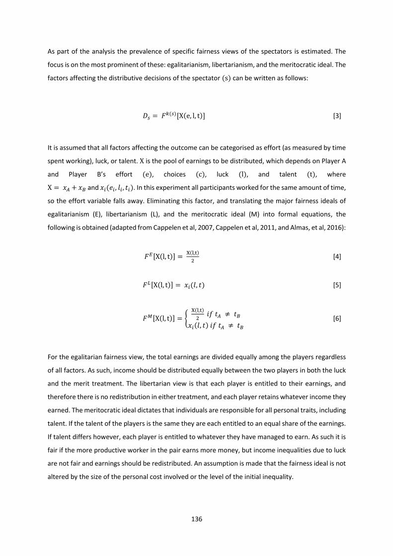
136
As part of the analysis the prevalence of specific fairness views of the spectators is estimated. The
focus is on the most prominent of these: egalitarianism, libertarianism, and the meritocratic ideal. The
factors affecting the distributive decisions of the spectator (s) can be written as follows:
𝐷𝑠 = 𝐹𝑘(𝑠)[X(e, l, t)] [3]
It is assumed that all factors affecting the outcome can be categorised as effort (as measured by time
spent working), luck, or talent. X is the pool of earnings to be distributed, which depends on Player A
and Player B’s effort (e), choices (c), luck (l), and talent (t), where
X = 𝑥𝐴 + 𝑥𝐵 and 𝑥𝑖(𝑒𝑖, 𝑙𝑖, 𝑡𝑖). In this experiment all participants worked for the same amount of time,
so the effort variable falls away. Eliminating this factor, and translating the major fairness ideals of
egalitarianism (E), libertarianism (L), and the meritocratic ideal (M) into formal equations, the
following is obtained (adapted from Cappelen et al, 2007, Cappelen et al, 2011, and Almas, et al, 2016):
𝐹𝐸[X(l, t)] = X(l,t)
2 [4]
𝐹𝐿[X(l, t)] = 𝑥𝑖(𝑙, 𝑡) [5]
𝐹𝑀[X(l, t)] = {X(l,t)
2 𝑖𝑓 𝑡𝐴 ≠ 𝑡𝐵
𝑥𝑖(𝑙, 𝑡) 𝑖𝑓 𝑡𝐴 ≠ 𝑡𝐵
[6]
For the egalitarian fairness view, the total earnings are divided equally among the players regardless
of all factors. As such, income should be distributed equally between the two players in both the luck
and the merit treatment. The libertarian view is that each player is entitled to their earnings, and
therefore there is no redistribution in either treatment, and each player retains whatever income they
earned. The meritocratic ideal dictates that individuals are responsible for all personal traits, including
talent. If the talent of the players is the same they are each entitled to an equal share of the earnings.
If talent differs however, each player is entitled to whatever they have managed to earn. As such it is
fair if the more productive worker in the pair earns more money, but income inequalities due to luck
are not fair and earnings should be redistributed. An assumption is made that the fairness ideal is not
altered by the size of the personal cost involved or the level of the initial inequality.
137
Differences between the luck and the merit treatment in the choice of whether to redistribute or not
are thus driven by spectators with a meritocratic fairness ideal. Libertarian spectators do not face a
trade-off between fairness considerations and self-interest considerations in terms of the personal
cost of redistribution, since for them the fair choice of not redistributing coincides with no personal
cost. As such, the effect of a personal cost depends both on the proportion of spectators holding non-
libertarian fairness views, and on the relative importance these spectators assign to self-interest.
6.4.3 Experimental Procedure
Experiment material
The development of the material for the experiment included mini pilot studies of both worker and
spectator sessions. The purpose of these pilots was to test the planned experiment and identify any
issues in the instructions or tasks to be performed by participants. Discussions were conducted
following each pilot session to explore any misunderstandings or misinterpretations of the
experiment. There were numerous iterations over which the instructions, tasks, and the survey were
tested and revised. These pilot sessions included individuals of various ages and educational
backgrounds to get varied perspectives on how clear the instructions and tasks were, as well as how
long each session was likely to take.
As part of the full experiment the instructions were read aloud by the facilitator at the start of each
session to assist in clarity of understanding. Following this, and before commencing with the tasks or
decision making, participants were asked to raise their hand if they had any questions, which were
then answered individually by the facilitator. There were only a handful of questions across all the
sessions conducted.
Recruitment
Students were recruited from the population of the University of Cape Town students. The university
had a total of 26 116 students enrolled in 2013, comprising 6 119 Africans, 3 573 coloureds, 1 715
Indians, 8 434 whites, 1 488 others, and 4 708 internationals.57 An email was sent to all students across
57 Most current 2013 statistics available from http://www.uct.ac.za/about/intro/statistics/
138
all faculties a few days prior to the first session to obtain a sample that is as representative of the
university as possible. The email gave vague indications about what would be required, and that
participants could earn up to R120 for their time. There was an over subscription by more than 200%,
and places in each session were allocated on a first come first served basis. The sessions were
conducted at various times on various days so as not to exclude any particular group of students. In
total, five sessions were conducted from 2 October 2015 to 8 October 2015. The first three sessions
were worker sessions, with the last two sessions being spectator sessions. When signing up, students
were not informed about which session they would be attending, or how the sessions differed58. All
the sessions took place in lecture venues at the university.
In total of 335 students took part in the study, with 219 workers and 116 spectators. The spectator
sample is of primary interest for the experiment and will be examined in detail, with only a brief
explanation of the production phase.
The Production Phase
Participants in these sessions were asked to work on a set of assignments, including numerical and
grammar tasks. The total time required, including going through instructions and working on the tasks,
was approximately 30 minutes. This is roughly the same amount of time as the decision-making
sessions. Participants were informed that the amount they earn may be determined by their
productivity, and that ultimately it is determined by an anonymous third party. They were not
informed about which treatment group they were in as this had not yet been determined. The full
instructions, as well as the tasks, are included in Appendix A6.1. Following the session, workers were
randomly split into the two treatment groups, randomly paired, and each pair was then matched with
a spectator in the same treatment group. In the Luck treatment the winner and loser were determined
by a random lottery, with the winner being Player A and the loser being Player B. In the Merit
treatment the task scores of the pair were compared, with the most productive player (achieving the
higher score) being Player A and the less productive player being Player B. The spectator with which
the workers were paired ultimately determined the amount that each participant would earn.
58 The sessions were all completed before the disruption of university activities as a result of the #FeesMustFall protests.
139
The Decision-making Phase
Randomisation took place immediately prior to the spectator sessions, which followed the production
phase. On arrival participants gathered outside the lecture venue. They were then instructed to pick
a coloured marble out of a bag without looking, with equal numbers of green and brown marbles.
Once selection began, participants were instructed that they may not communicate. The colour of the
marble determined the treatment group, with green denoting Merit and brown Luck. Participants all
revealed their marble at the same time, and were then directed to the appropriate adjacent venue.
Participants were not aware of how the two groups differed, or why exactly the marble selection took
place.
This within session randomisation increases the validity of the experiment in comparison to
experiments where each session is allocated to one treatment. This is because the choice of session
may not be completely random, with various observable and unobservable factors at play. For
example, Friday prayers would prevent all Muslim participants from attending the Friday 1pm session.
By randomising within session, such systematic difference between treatment groups are minimised.
The decision-making phase comprised two parts. In the first part spectators made a set of incentivised
redistributive choices regarding the income of the workers they are paired with. In the second part
spectators completed a non-incentivised survey questionnaire, including questions about their
attitude towards redistributive policies and standard background questions. All the instructions,
decision tables, and surveys were printed and completed by hand. No one was allowed to leave the
venue during a session, and all participants stayed until the end. Sessions were approximately 30 to
35 minutes long, depending on how quickly the questions were answered. The redistributive decisions
of the spectators are of primary interest, and the process is explained in detail.
Distributive choice
In the first part the spectators made a series of redistributive decisions on the income of a pair of
workers. The context of each decision varied in terms of the size of the initial inequality in the payment
split between Player A and Player B, and in the potential cost to the spectator. This is outlined in detail
in the instructions. Below are the instructions for the Merit treatment, with the Luck treatment
instructions only differing in the determination of Player A and Player B by a lottery rather than relative
productivity. The full Luck treatment instructions can be found in Appendix A6.1.
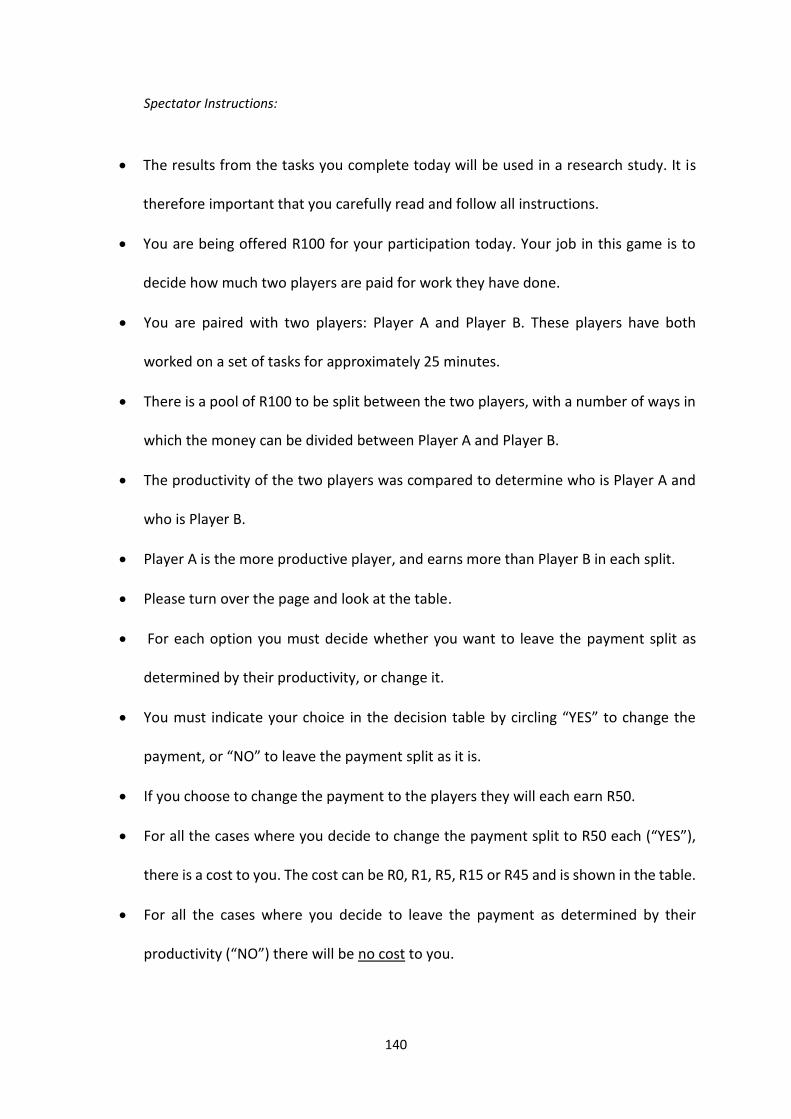
140
Spectator Instructions:
• The results from the tasks you complete today will be used in a research study. It is
therefore important that you carefully read and follow all instructions.
• You are being offered R100 for your participation today. Your job in this game is to
decide how much two players are paid for work they have done.
• You are paired with two players: Player A and Player B. These players have both
worked on a set of tasks for approximately 25 minutes.
• There is a pool of R100 to be split between the two players, with a number of ways in
which the money can be divided between Player A and Player B.
• The productivity of the two players was compared to determine who is Player A and
who is Player B.
• Player A is the more productive player, and earns more than Player B in each split.
• Please turn over the page and look at the table.
• For each option you must decide whether you want to leave the payment split as
determined by their productivity, or change it.
• You must indicate your choice in the decision table by circling “YES” to change the
payment, or “NO” to leave the payment split as it is.
• If you choose to change the payment to the players they will each earn R50.
• For all the cases where you decide to change the payment split to R50 each (“YES”),
there is a cost to you. The cost can be R0, R1, R5, R15 or R45 and is shown in the table.
• For all the cases where you decide to leave the payment as determined by their
productivity (“NO”) there will be no cost to you.
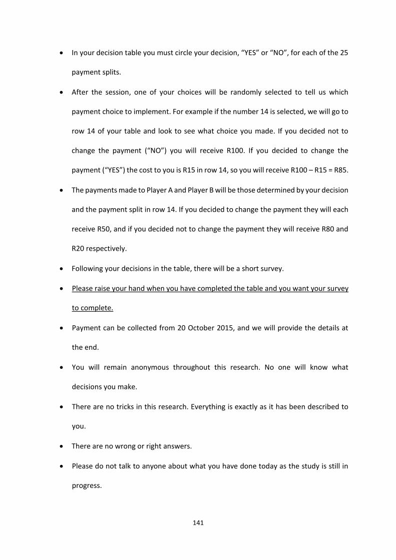
141
• In your decision table you must circle your decision, “YES” or “NO”, for each of the 25
payment splits.
• After the session, one of your choices will be randomly selected to tell us which
payment choice to implement. For example if the number 14 is selected, we will go to
row 14 of your table and look to see what choice you made. If you decided not to
change the payment (“NO”) you will receive R100. If you decided to change the
payment (“YES”) the cost to you is R15 in row 14, so you will receive R100 – R15 = R85.
• The payments made to Player A and Player B will be those determined by your decision
and the payment split in row 14. If you decided to change the payment they will each
receive R50, and if you decided not to change the payment they will receive R80 and
R20 respectively.
• Following your decisions in the table, there will be a short survey.
• Please raise your hand when you have completed the table and you want your survey
to complete.
• Payment can be collected from 20 October 2015, and we will provide the details at
the end.
• You will remain anonymous throughout this research. No one will know what
decisions you make.
• There are no tricks in this research. Everything is exactly as it has been described to
you.
• There are no wrong or right answers.
• Please do not talk to anyone about what you have done today as the study is still in
progress.
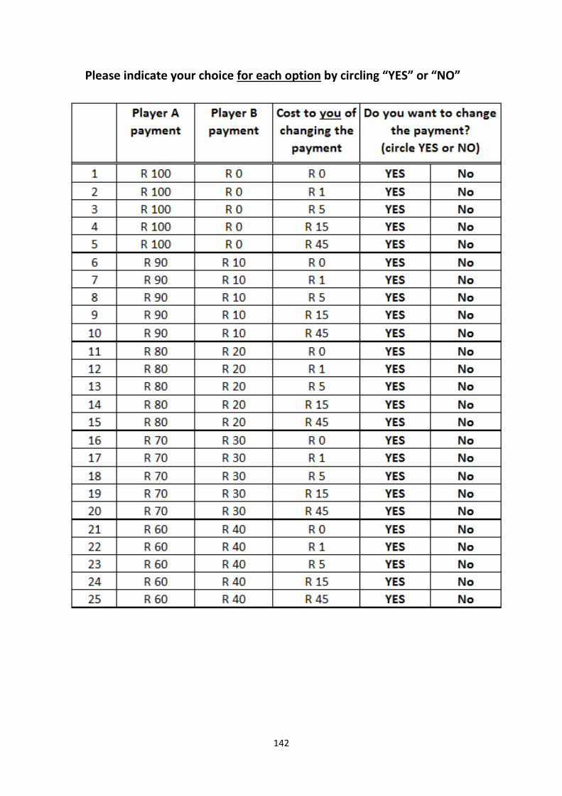
142
Please indicate your choice for each option by circling “YES” or “NO”
143
In sum, each spectator made a series of 25 decisions about the distribution of the pooled income
between the pair of workers. One of the decisions was randomly chosen as the actual payments made
to the workers and the spectator.
There were two possible outcomes for each decision made by the spectator:
1) The spectator chooses not to redistribute, there is no cost to him/her, and there is some
resultant inequality in the income earned by the two workers.
2) The spectator chooses to redistribute, there is some associated cost to the spectator (R0, R1,
R5, R15 or R45), and there is no difference between the income of the two workers (R50 each).
The cost of R1 is included in the table as a negligible amount to differentiate between purely selfish
individuals, and those that value fairness minimally. When there is no cist it is not clear whether a
purely selfish individual would choose to redistribute or not, as their utility is maximised either way.
It can be argued that the redistributive choices made by such individuals, when no cost is involved, is
purely random. As such, nothing can be said about their preferences for fairness as the choice made
is arbitrary and not necessarily an indication of their preference. However, when the cost is R1, an
arguably negligible amount, purely selfish individuals will consistently choose to not redistribute, while
those with even a small preference for fairness are more likely to redistribute.
The survey
Following the decision making, participants completed a short survey. The decision tables were
collected from the participants prior to the completion of the survey to prevent any changes in the
decisions which may have been prompted by the survey questions. In particular, the three questions
about the role of luck, effort, government, and society in determining income may have effected a
change of heart regarding the decisions made. While it is possible that the answers to these questions
were primed by the decisions that were made, this is less of a problem than the reverse as the
redistributive decisions are of primary interest in this study.
144
Research questions
The experiment is designed to study social preferences regarding fairness and redistribution. The focus
is on analysing how levels of initial inequality and the personal cost involved affect redistributive
choices, as well as the impact of the source of the inequality.
Inequality level and cost
Two of the key questions are how initial inequality and the personal cost involved affect inequality
acceptance. The initial inequality varies in size from complete inequality on the one hand, where one
workers is allocated all the income while the other receives nothing, to minimal inequality where
incomes are similar. The personal cost of redistribution varies from no cost to 45% of the spectator’s
earnings.
Question 1: Do higher initial inequality levels reduce inequality acceptance and result in a higher
proportion of decisions to redistribute?
Question 2: Do higher personal costs increase inequality acceptance and result in a lower proportion
of decisions to redistribute?
Luck and merit
The experiment is divided into two treatments where the impact of luck and merit as sources of
inequality are considered separately. A meritocratic society will have higher levels of inequality
acceptance than, say, an egalitarian society. If participants are meritocratic, it is expected that higher
inequality acceptance will be observed in the Merit treatment.
Question 3: Is inequality acceptance higher in the Merit treatment than in the Luck treatment (i.e.
lower level of redistribution taking place in the Merit treatment)?
145
Heterogeneity
The experiment also considers heterogeneity in social preferences using the background data
collected in the survey, where the focus is on race, gender, and socioeconomic status. Significant
differences between these socio-demographic groups will be tested for.
Attitudes to redistribution
Lastly the experiment will explore how the distributive choices of the spectators relate to responses
to the survey questions about their attitude towards redistributive policies. This will be discussed with
reference to findings in the World Values Survey for South Africa.
6.5 Main Analysis and Results
Various summary statistics of the spectator choices in the two treatments are presented first. The
main regressions estimating the logit marginal effects are discussed next, followed by elasticity
comparisons, and the prevalence of the three fairness views.
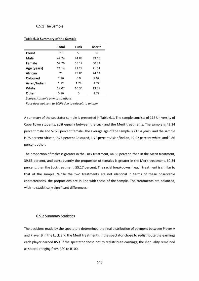
146
6.5.1 The Sample
Table 6.1: Summary of the Sample
Total Luck Merit
Count 116 58 58
Male 42.24 44.83 39.66
Female 57.76 55.17 60.34
Age (years) 21.14 21.28 21.01
African 75 75.86 74.14
Coloured 7.76 6.9 8.62
Asian/Indian 1.72 1.72 1.72
White 12.07 10.34 13.79
Other 0.86 0 1.72
Source: Author’s own calculations.
Race does not sum to 100% due to refusals to answer
A summary of the spectator sample is presented in Table 6.1. The sample consists of 116 University of
Cape Town students, split equally between the Luck and the Merit treatments. The sample is 42.24
percent male and 57.76 percent female. The average age of the sample is 21.14 years, and the sample
is 75 percent African, 7.76 percent Coloured, 1.72 percent Asian/Indian, 12.07 percent white, and 0.86
percent other.
The proportion of males is greater in the Luck treatment, 44.83 percent, than in the Merit treatment,
39.66 percent, and consequently the proportion of females is greater in the Merit treatment, 60.34
percent, than the Luck treatment, 55.17 percent. The racial breakdown in each treatment is similar to
that of the sample. While the two treatments are not identical in terms of these observable
characteristics, the proportions are in line with those of the sample. The treatments are balanced,
with no statistically significant differences.
6.5.2 Summary Statistics
The decisions made by the spectators determined the final distribution of payment between Player A
and Player B in the Luck and the Merit treatments. If the spectator chose to redistribute the earnings
each player earned R50. If the spectator chose not to redistribute earnings, the inequality remained
as stated, ranging from R20 to R100.
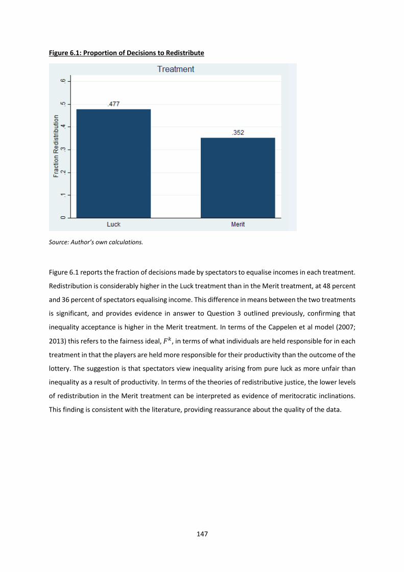
147
Figure 6.1: Proportion of Decisions to Redistribute
Source: Author’s own calculations.
Figure 6.1 reports the fraction of decisions made by spectators to equalise incomes in each treatment.
Redistribution is considerably higher in the Luck treatment than in the Merit treatment, at 48 percent
and 36 percent of spectators equalising income. This difference in means between the two treatments
is significant, and provides evidence in answer to Question 3 outlined previously, confirming that
inequality acceptance is higher in the Merit treatment. In terms of the Cappelen et al model (2007;
2013) this refers to the fairness ideal, 𝐹𝑘, in terms of what individuals are held responsible for in each
treatment in that the players are held more responsible for their productivity than the outcome of the
lottery. The suggestion is that spectators view inequality arising from pure luck as more unfair than
inequality as a result of productivity. In terms of the theories of redistributive justice, the lower levels
of redistribution in the Merit treatment can be interpreted as evidence of meritocratic inclinations.
This finding is consistent with the literature, providing reassurance about the quality of the data.
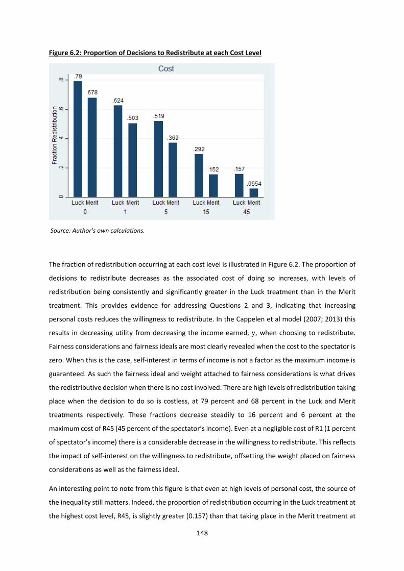
148
Figure 6.2: Proportion of Decisions to Redistribute at each Cost Level
Source: Author’s own calculations.
The fraction of redistribution occurring at each cost level is illustrated in Figure 6.2. The proportion of
decisions to redistribute decreases as the associated cost of doing so increases, with levels of
redistribution being consistently and significantly greater in the Luck treatment than in the Merit
treatment. This provides evidence for addressing Questions 2 and 3, indicating that increasing
personal costs reduces the willingness to redistribute. In the Cappelen et al model (2007; 2013) this
results in decreasing utility from decreasing the income earned, y, when choosing to redistribute.
Fairness considerations and fairness ideals are most clearly revealed when the cost to the spectator is
zero. When this is the case, self-interest in terms of income is not a factor as the maximum income is
guaranteed. As such the fairness ideal and weight attached to fairness considerations is what drives
the redistributive decision when there is no cost involved. There are high levels of redistribution taking
place when the decision to do so is costless, at 79 percent and 68 percent in the Luck and Merit
treatments respectively. These fractions decrease steadily to 16 percent and 6 percent at the
maximum cost of R45 (45 percent of the spectator’s income). Even at a negligible cost of R1 (1 percent
of spectator’s income) there is a considerable decrease in the willingness to redistribute. This reflects
the impact of self-interest on the willingness to redistribute, offsetting the weight placed on fairness
considerations as well as the fairness ideal.
An interesting point to note from this figure is that even at high levels of personal cost, the source of
the inequality still matters. Indeed, the proportion of redistribution occurring in the Luck treatment at
the highest cost level, R45, is slightly greater (0.157) than that taking place in the Merit treatment at
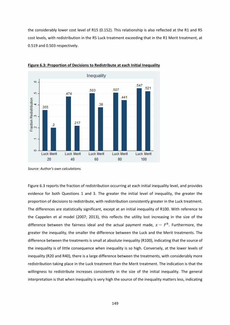
149
the considerably lower cost level of R15 (0.152). This relationship is also reflected at the R1 and R5
cost levels, with redistribution in the R5 Luck treatment exceeding that in the R1 Merit treatment, at
0.519 and 0.503 respectively.
Figure 6.3: Proportion of Decisions to Redistribute at each Initial Inequality
Source: Author’s own calculations.
Figure 6.3 reports the fraction of redistribution occurring at each initial inequality level, and provides
evidence for both Questions 1 and 3. The greater the initial level of inequality, the greater the
proportion of decisions to redistribute, with redistribution consistently greater in the Luck treatment.
The differences are statistically significant, except at an initial inequality of R100. With reference to
the Cappelen et al model (2007; 2013), this reflects the utility lost increasing in the size of the
difference between the fairness ideal and the actual payment made, 𝑥 − 𝐹𝑘. Furthermore, the
greater the inequality, the smaller the difference between the Luck and the Merit treatments. The
difference between the treatments is small at absolute inequality (R100), indicating that the source of
the inequality is of little consequence when inequality is so high. Conversely, at the lower levels of
inequality (R20 and R40), there is a large difference between the treatments, with considerably more
redistribution taking place in the Luck treatment than the Merit treatment. The indication is that the
willingness to redistribute increases consistently in the size of the initial inequality. The general
interpretation is that when inequality is very high the source of the inequality matters less, indicating
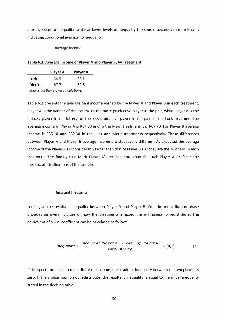
150
pure aversion to inequality, while at lower levels of inequality the source becomes more relevant,
indicating conditional aversion to inequality.
Average Income
Table 6.2: Average Income of Player A and Player B, by Treatment
Player A Player B
Luck 64.9 35.1
Merit 67.7 32.3
Source: Author’s own calculations.
Table 6.2 presents the average final income earned by the Player A and Player B in each treatment.
Player A is the winner of the lottery, or the more productive player in the pair, while Player B is the
unlucky player in the lottery, or the less productive player in the pair. In the Luck treatment the
average income of Player A is R64.90 and in the Merit treatment it is R67.70. For Player B average
income is R35.10 and R32.30 in the Luck and Merit treatments respectively. These differences
between Player A and Player B average income are statistically different. As expected the average
income of the Player A’s is considerably larger than that of Player B’s as they are the ‘winners’ in each
treatment. The finding that Merit Player A’s receive more than the Luck Player A’s reflects the
meritocratic inclinations of the sample.
Resultant Inequality
Looking at the resultant inequality between Player A and Player B after the redistribution phase
provides an overall picture of how the treatments affected the willingness to redistribute. The
equivalent of a Gini coefficient can be calculated as follows:
Inequality = |𝐼𝑛𝑐𝑜𝑚𝑒 𝑜𝑓 𝑃𝑙𝑎𝑦𝑒𝑟 𝐴 − 𝐼𝑛𝑐𝑜𝑚𝑒 𝑜𝑓 𝑃𝑙𝑎𝑦𝑒𝑟 𝐵|
𝑇𝑜𝑡𝑎𝑙 𝐼𝑛𝑐𝑜𝑚𝑒 ∈ [0,1] [7]
If the spectator chose to redistribute the income, the resultant inequality between the two players is
zero. If the choice was to not redistribute, the resultant inequality is equal to the initial inequality
stated in the decision table.
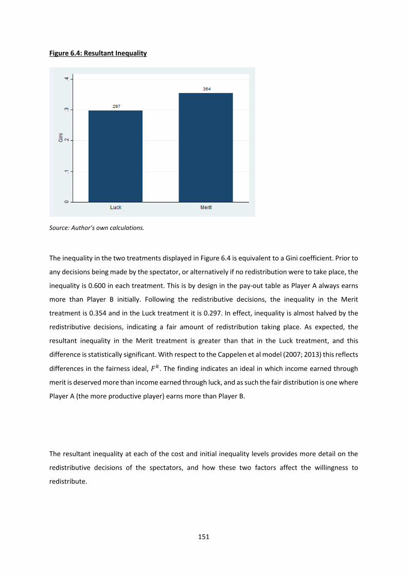
151
Figure 6.4: Resultant Inequality
Source: Author’s own calculations.
The inequality in the two treatments displayed in Figure 6.4 is equivalent to a Gini coefficient. Prior to
any decisions being made by the spectator, or alternatively if no redistribution were to take place, the
inequality is 0.600 in each treatment. This is by design in the pay-out table as Player A always earns
more than Player B initially. Following the redistributive decisions, the inequality in the Merit
treatment is 0.354 and in the Luck treatment it is 0.297. In effect, inequality is almost halved by the
redistributive decisions, indicating a fair amount of redistribution taking place. As expected, the
resultant inequality in the Merit treatment is greater than that in the Luck treatment, and this
difference is statistically significant. With respect to the Cappelen et al model (2007; 2013) this reflects
differences in the fairness ideal, 𝐹𝑘. The finding indicates an ideal in which income earned through
merit is deserved more than income earned through luck, and as such the fair distribution is one where
Player A (the more productive player) earns more than Player B.
The resultant inequality at each of the cost and initial inequality levels provides more detail on the
redistributive decisions of the spectators, and how these two factors affect the willingness to
redistribute.
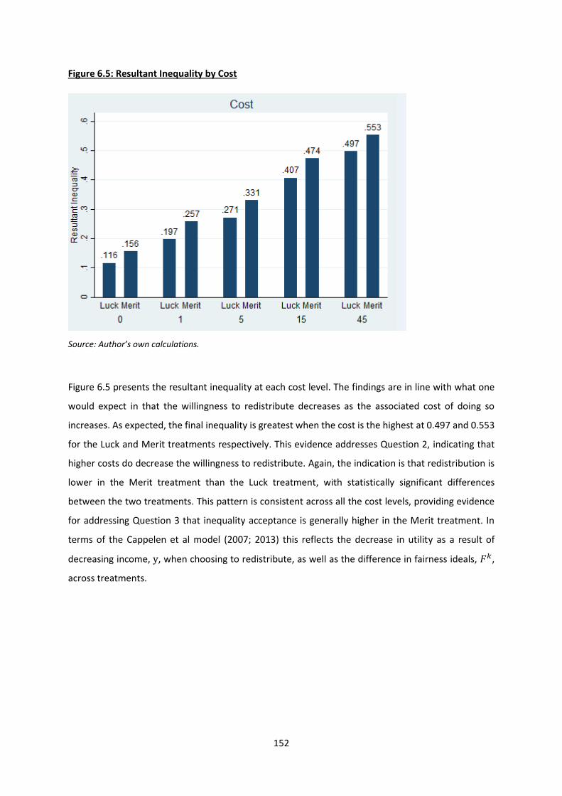
152
Figure 6.5: Resultant Inequality by Cost
Source: Author’s own calculations.
Figure 6.5 presents the resultant inequality at each cost level. The findings are in line with what one
would expect in that the willingness to redistribute decreases as the associated cost of doing so
increases. As expected, the final inequality is greatest when the cost is the highest at 0.497 and 0.553
for the Luck and Merit treatments respectively. This evidence addresses Question 2, indicating that
higher costs do decrease the willingness to redistribute. Again, the indication is that redistribution is
lower in the Merit treatment than the Luck treatment, with statistically significant differences
between the two treatments. This pattern is consistent across all the cost levels, providing evidence
for addressing Question 3 that inequality acceptance is generally higher in the Merit treatment. In
terms of the Cappelen et al model (2007; 2013) this reflects the decrease in utility as a result of
decreasing income, y, when choosing to redistribute, as well as the difference in fairness ideals, 𝐹𝑘,
across treatments.
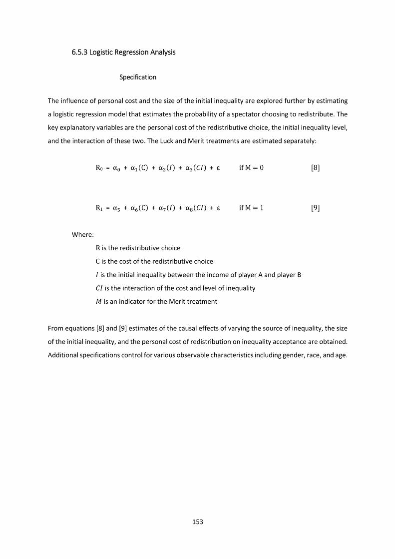
153
6.5.3 Logistic Regression Analysis
Specification
The influence of personal cost and the size of the initial inequality are explored further by estimating
a logistic regression model that estimates the probability of a spectator choosing to redistribute. The
key explanatory variables are the personal cost of the redistributive choice, the initial inequality level,
and the interaction of these two. The Luck and Merit treatments are estimated separately:
R0 = α0 + α1(C) + α2(𝐼) + α3(𝐶𝐼) + ɛ if M = 0 [8]
R1 = α5 + α6(C) + α7(𝐼) + α8(𝐶𝐼) + ɛ if M = 1 [9]
Where:
R is the redistributive choice
C is the cost of the redistributive choice
𝐼 is the initial inequality between the income of player A and player B
𝐶𝐼 is the interaction of the cost and level of inequality
𝑀 is an indicator for the Merit treatment
From equations [8] and [9] estimates of the causal effects of varying the source of inequality, the size
of the initial inequality, and the personal cost of redistribution on inequality acceptance are obtained.
Additional specifications control for various observable characteristics including gender, race, and age.
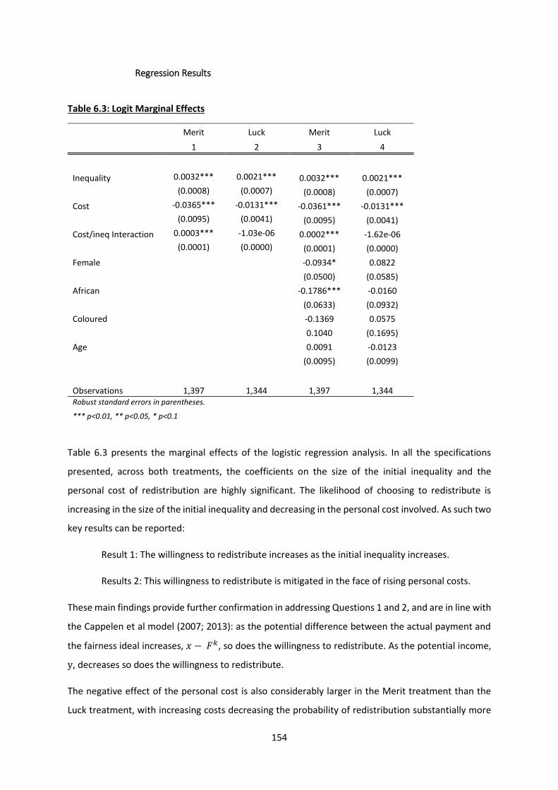
154
Regression Results
Table 6.3: Logit Marginal Effects
Merit Luck Merit Luck
1 2 3 4
Inequality 0.0032*** 0.0021*** 0.0032*** 0.0021***
(0.0008) (0.0007) (0.0008) (0.0007)
Cost -0.0365*** -0.0131*** -0.0361*** -0.0131***
(0.0095) (0.0041) (0.0095) (0.0041)
Cost/ineq Interaction 0.0003*** -1.03e-06 0.0002*** -1.62e-06
(0.0001) (0.0000) (0.0001) (0.0000)
Female -0.0934* 0.0822
(0.0500) (0.0585)
African -0.1786*** -0.0160
(0.0633) (0.0932)
Coloured -0.1369 0.0575
0.1040 (0.1695)
Age 0.0091 -0.0123
(0.0095) (0.0099)
Observations 1,397 1,344 1,397 1,344 Robust standard errors in parentheses.
*** p<0.01, ** p<0.05, * p<0.1
Table 6.3 presents the marginal effects of the logistic regression analysis. In all the specifications
presented, across both treatments, the coefficients on the size of the initial inequality and the
personal cost of redistribution are highly significant. The likelihood of choosing to redistribute is
increasing in the size of the initial inequality and decreasing in the personal cost involved. As such two
key results can be reported:
Result 1: The willingness to redistribute increases as the initial inequality increases.
Results 2: This willingness to redistribute is mitigated in the face of rising personal costs.
These main findings provide further confirmation in addressing Questions 1 and 2, and are in line with
the Cappelen et al model (2007; 2013): as the potential difference between the actual payment and
the fairness ideal increases, 𝑥 − 𝐹𝑘, so does the willingness to redistribute. As the potential income,
y, decreases so does the willingness to redistribute.
The negative effect of the personal cost is also considerably larger in the Merit treatment than the
Luck treatment, with increasing costs decreasing the probability of redistribution substantially more
155
in the Merit treatment59. Considering the interpretation that inequality arising from luck is more unfair
than that arising from merit, the negative impact of the cost involved has less of a bearing when the
source is deemed unfair. This is in line with the intuition that people are willing to sacrifice more in
the face of greater perceived unfairness. Thus, as a further result:
Result 3: Self-interest considerations carry less weight when the source of the inequality is
deemed unfair, resulting in a greater probability of redistribution.
The interaction term of cost and inequality in the Merit treatment, while small, is significantly positive.
The interaction term is not significant in the Luck treatment. This indicates two additional results:
Result 4a: The effect of the size of the inequality is increasing in the cost involved in the Merit
treatment.
Result 4b: The source of the inequality makes a difference in how personal cost and the size
of the inequality interact.
In terms of the heterogeneous effects, females are significantly less likely than males to redistribute
in the Merit treatment, while gender is not significant in the Luck treatment. This is interesting, as it
indicates that females believe that players in the Merit treatment are responsible for their allocated
earnings more strongly than males. While a significant gender covariate is common in the literature,
the more common finding is that females are more likely to redistribute than males.60 Africans are
also significantly less likely to redistribute than whites in the Merit treatment, but not in the Luck
treatment.61 As such, Africans in our sample are significantly less likely to redistribute earnings than
any other population group. It can therefore be inferred that in our sample Africans and females have
a stronger belief that individuals are responsible for their productivity and resultant earnings. Finally,
age does not have a significant effect in either treatment.
59 The cost coefficients in the two treatments are significantly different at the 5% level. 60 See for example Cappelen et al 2014 & 2010; Durante, Putterman & van der Weele, 2014. 61 The race variables Indian/Asian and Other have been excluded from the analysis as there are only three
observations in total and this is not big enough for clustering at the spectator level. There are 3 spectators who refused to answer the race question and have also been excluded from the regression analysis. This results in a sample of 110 spectators, 54 in the Luck treatment and 56 in the Merit treatment.
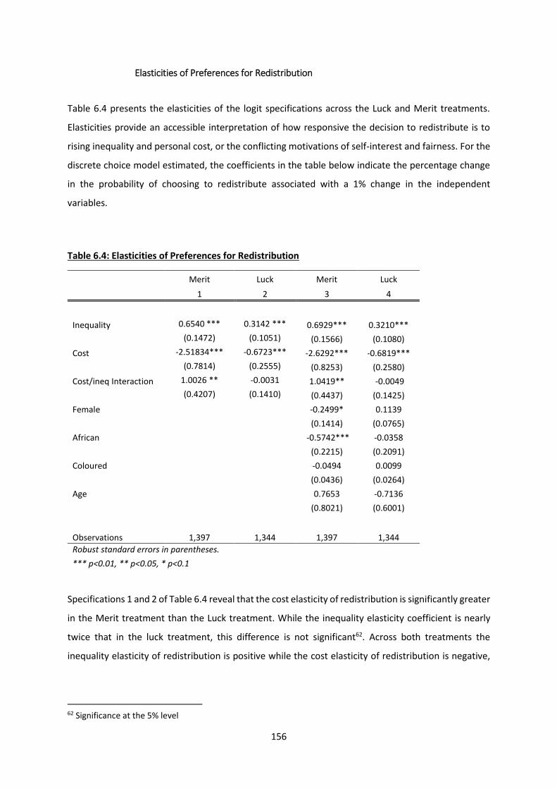
156
Elasticities of Preferences for Redistribution
Table 6.4 presents the elasticities of the logit specifications across the Luck and Merit treatments.
Elasticities provide an accessible interpretation of how responsive the decision to redistribute is to
rising inequality and personal cost, or the conflicting motivations of self-interest and fairness. For the
discrete choice model estimated, the coefficients in the table below indicate the percentage change
in the probability of choosing to redistribute associated with a 1% change in the independent
variables.
Table 6.4: Elasticities of Preferences for Redistribution
Merit Luck Merit Luck
1 2 3 4
Inequality 0.6540 *** 0.3142 *** 0.6929*** 0.3210***
(0.1472) (0.1051) (0.1566) (0.1080)
Cost -2.51834*** -0.6723*** -2.6292*** -0.6819***
(0.7814) (0.2555) (0.8253) (0.2580)
Cost/ineq Interaction 1.0026 ** -0.0031 1.0419** -0.0049
(0.4207) (0.1410) (0.4437) (0.1425)
Female -0.2499* 0.1139
(0.1414) (0.0765)
African -0.5742*** -0.0358
(0.2215) (0.2091)
Coloured -0.0494 0.0099
(0.0436) (0.0264)
Age 0.7653 -0.7136
(0.8021) (0.6001)
Observations 1,397 1,344 1,397 1,344
Robust standard errors in parentheses.
*** p<0.01, ** p<0.05, * p<0.1
Specifications 1 and 2 of Table 6.4 reveal that the cost elasticity of redistribution is significantly greater
in the Merit treatment than the Luck treatment. While the inequality elasticity coefficient is nearly
twice that in the luck treatment, this difference is not significant62. Across both treatments the
inequality elasticity of redistribution is positive while the cost elasticity of redistribution is negative,
62 Significance at the 5% level
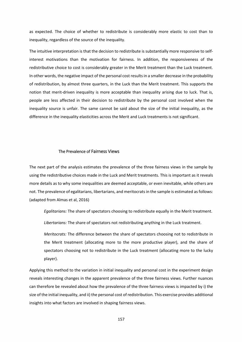
157
as expected. The choice of whether to redistribute is considerably more elastic to cost than to
inequality, regardless of the source of the inequality.
The intuitive interpretation is that the decision to redistribute is substantially more responsive to self-
interest motivations than the motivation for fairness. In addition, the responsiveness of the
redistributive choice to cost is considerably greater in the Merit treatment than the Luck treatment.
In other words, the negative impact of the personal cost results in a smaller decrease in the probability
of redistribution, by almost three quarters, in the Luck than the Merit treatment. This supports the
notion that merit-driven inequality is more acceptable than inequality arising due to luck. That is,
people are less affected in their decision to redistribute by the personal cost involved when the
inequality source is unfair. The same cannot be said about the size of the initial inequality, as the
difference in the inequality elasticities across the Merit and Luck treatments is not significant.
The Prevalence of Fairness Views
The next part of the analysis estimates the prevalence of the three fairness views in the sample by
using the redistributive choices made in the Luck and Merit treatments. This is important as it reveals
more details as to why some inequalities are deemed acceptable, or even inevitable, while others are
not. The prevalence of egalitarians, libertarians, and meritocrats in the sample is estimated as follows:
(adapted from Almas et al, 2016)
Egalitarians: The share of spectators choosing to redistribute equally in the Merit treatment.
Libertarians: The share of spectators not redistributing anything in the Luck treatment.
Meritocrats: The difference between the share of spectators choosing not to redistribute in
the Merit treatment (allocating more to the more productive player), and the share of
spectators choosing not to redistribute in the Luck treatment (allocating more to the lucky
player).
Applying this method to the variation in initial inequality and personal cost in the experiment design
reveals interesting changes in the apparent prevalence of the three fairness views. Further nuances
can therefore be revealed about how the prevalence of the three fairness views is impacted by i) the
size of the initial inequality, and ii) the personal cost of redistribution. This exercise provides additional
insights into what factors are involved in shaping fairness views.
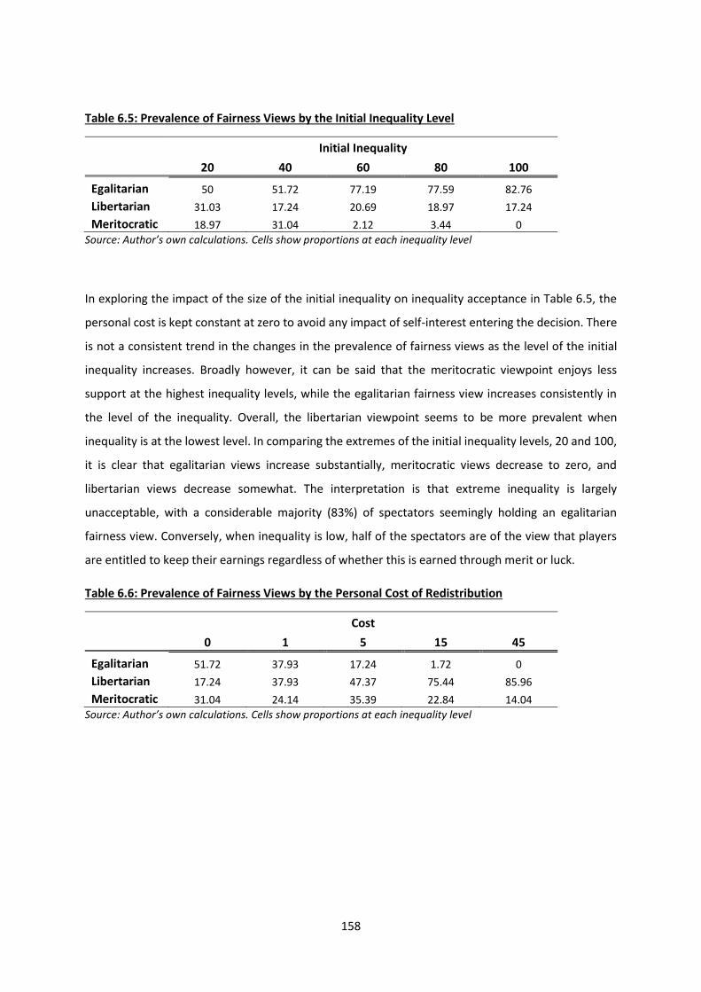
158
Table 6.5: Prevalence of Fairness Views by the Initial Inequality Level
Initial Inequality
20 40 60 80 100
Egalitarian 50 51.72 77.19 77.59 82.76
Libertarian 31.03 17.24 20.69 18.97 17.24
Meritocratic 18.97 31.04 2.12 3.44 0
Source: Author’s own calculations. Cells show proportions at each inequality level
In exploring the impact of the size of the initial inequality on inequality acceptance in Table 6.5, the
personal cost is kept constant at zero to avoid any impact of self-interest entering the decision. There
is not a consistent trend in the changes in the prevalence of fairness views as the level of the initial
inequality increases. Broadly however, it can be said that the meritocratic viewpoint enjoys less
support at the highest inequality levels, while the egalitarian fairness view increases consistently in
the level of the inequality. Overall, the libertarian viewpoint seems to be more prevalent when
inequality is at the lowest level. In comparing the extremes of the initial inequality levels, 20 and 100,
it is clear that egalitarian views increase substantially, meritocratic views decrease to zero, and
libertarian views decrease somewhat. The interpretation is that extreme inequality is largely
unacceptable, with a considerable majority (83%) of spectators seemingly holding an egalitarian
fairness view. Conversely, when inequality is low, half of the spectators are of the view that players
are entitled to keep their earnings regardless of whether this is earned through merit or luck.
Table 6.6: Prevalence of Fairness Views by the Personal Cost of Redistribution
Cost
0 1 5 15 45
Egalitarian 51.72 37.93 17.24 1.72 0
Libertarian 17.24 37.93 47.37 75.44 85.96
Meritocratic 31.04 24.14 35.39 22.84 14.04
Source: Author’s own calculations. Cells show proportions at each inequality level
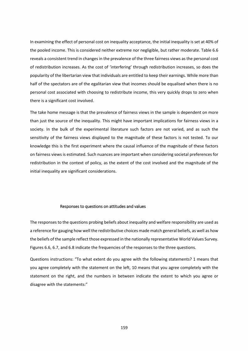
159
In examining the effect of personal cost on inequality acceptance, the initial inequality is set at 40% of
the pooled income. This is considered neither extreme nor negligible, but rather moderate. Table 6.6
reveals a consistent trend in changes in the prevalence of the three fairness views as the personal cost
of redistribution increases. As the cost of ‘interfering’ through redistribution increases, so does the
popularity of the libertarian view that individuals are entitled to keep their earnings. While more than
half of the spectators are of the egalitarian view that incomes should be equalised when there is no
personal cost associated with choosing to redistribute income, this very quickly drops to zero when
there is a significant cost involved.
The take home message is that the prevalence of fairness views in the sample is dependent on more
than just the source of the inequality. This might have important implications for fairness views in a
society. In the bulk of the experimental literature such factors are not varied, and as such the
sensitivity of the fairness views displayed to the magnitude of these factors is not tested. To our
knowledge this is the first experiment where the causal influence of the magnitude of these factors
on fairness views is estimated. Such nuances are important when considering societal preferences for
redistribution in the context of policy, as the extent of the cost involved and the magnitude of the
initial inequality are significant considerations.
Responses to questions on attitudes and values
The responses to the questions probing beliefs about inequality and welfare responsibility are used as
a reference for gauging how well the redistributive choices made match general beliefs, as well as how
the beliefs of the sample reflect those expressed in the nationally representative World Values Survey.
Figures 6.6, 6.7, and 6.8 indicate the frequencies of the responses to the three questions.
Questions instructions: “To what extent do you agree with the following statements? 1 means that
you agree completely with the statement on the left, 10 means that you agree completely with the
statement on the right, and the numbers in between indicate the extent to which you agree or
disagree with the statements:”
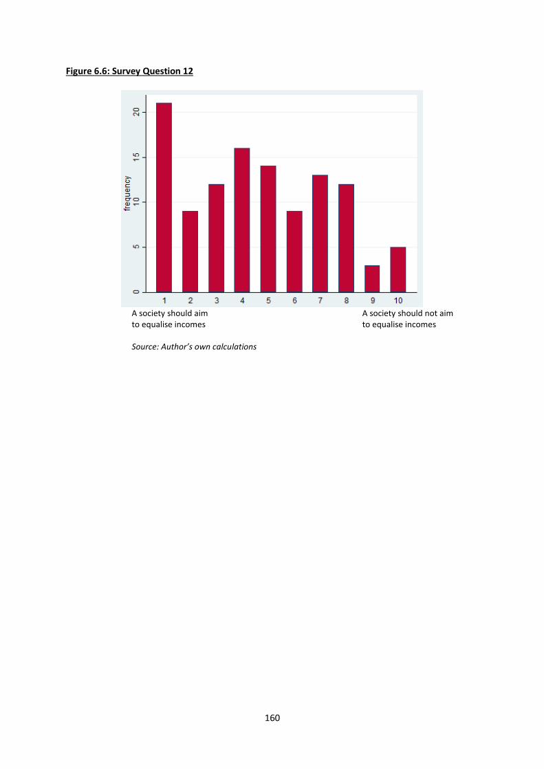
160
Figure 6.6: Survey Question 12
A society should aim A society should not aim to equalise incomes to equalise incomes Source: Author’s own calculations
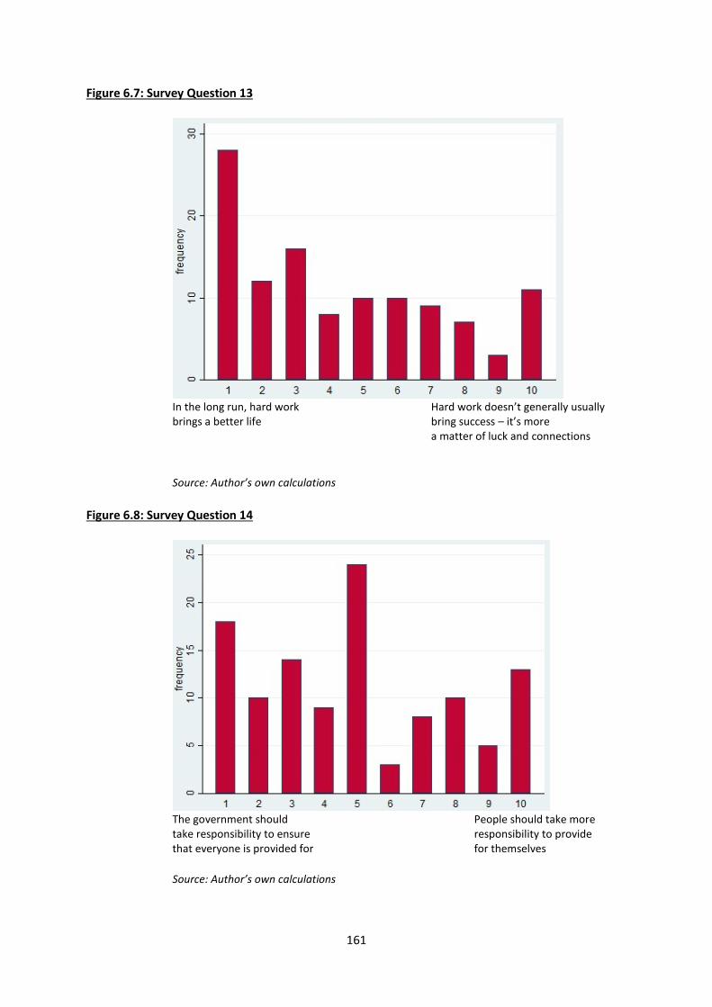
161
Figure 6.7: Survey Question 13
In the long run, hard work Hard work doesn’t generally usually brings a better life bring success – it’s more a matter of luck and connections
Source: Author’s own calculations
Figure 6.8: Survey Question 14
The government should People should take more take responsibility to ensure responsibility to provide that everyone is provided for for themselves Source: Author’s own calculations
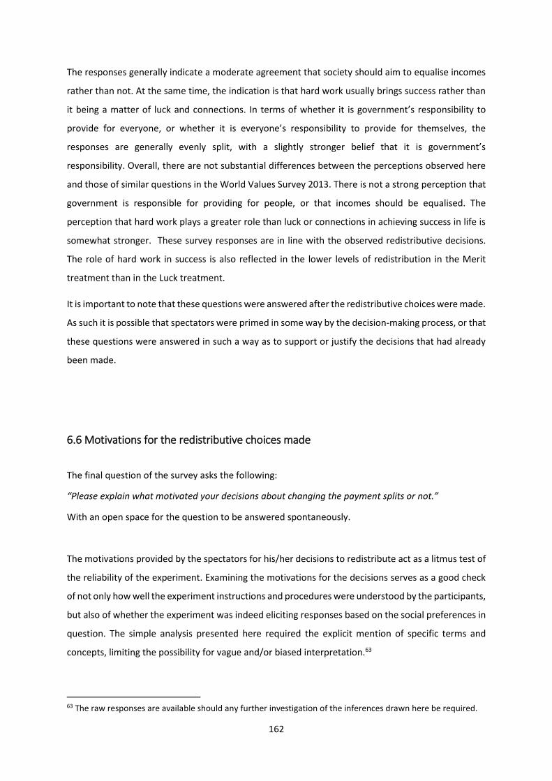
162
The responses generally indicate a moderate agreement that society should aim to equalise incomes
rather than not. At the same time, the indication is that hard work usually brings success rather than
it being a matter of luck and connections. In terms of whether it is government’s responsibility to
provide for everyone, or whether it is everyone’s responsibility to provide for themselves, the
responses are generally evenly split, with a slightly stronger belief that it is government’s
responsibility. Overall, there are not substantial differences between the perceptions observed here
and those of similar questions in the World Values Survey 2013. There is not a strong perception that
government is responsible for providing for people, or that incomes should be equalised. The
perception that hard work plays a greater role than luck or connections in achieving success in life is
somewhat stronger. These survey responses are in line with the observed redistributive decisions.
The role of hard work in success is also reflected in the lower levels of redistribution in the Merit
treatment than in the Luck treatment.
It is important to note that these questions were answered after the redistributive choices were made.
As such it is possible that spectators were primed in some way by the decision-making process, or that
these questions were answered in such a way as to support or justify the decisions that had already
been made.
6.6 Motivations for the redistributive choices made
The final question of the survey asks the following:
“Please explain what motivated your decisions about changing the payment splits or not.”
With an open space for the question to be answered spontaneously.
The motivations provided by the spectators for his/her decisions to redistribute act as a litmus test of
the reliability of the experiment. Examining the motivations for the decisions serves as a good check
of not only how well the experiment instructions and procedures were understood by the participants,
but also of whether the experiment was indeed eliciting responses based on the social preferences in
question. The simple analysis presented here required the explicit mention of specific terms and
concepts, limiting the possibility for vague and/or biased interpretation.63
63 The raw responses are available should any further investigation of the inferences drawn here be required.
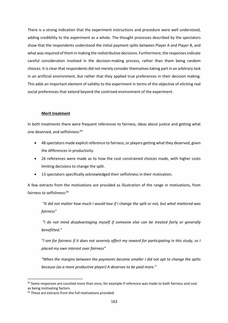
163
There is a strong indication that the experiment instructions and procedure were well understood,
adding credibility to the experiment as a whole. The thought processes described by the spectators
show that the respondents understood the initial payment splits between Player A and Player B, and
what was required of them in making the redistributive decisions. Furthermore, the responses indicate
careful consideration involved in the decision-making process, rather than them being random
choices. It is clear that respondents did not merely consider themselves taking part in an arbitrary task
in an artificial environment, but rather that they applied true preferences in their decision making.
This adds an important element of validity to the experiment in terms of the objective of eliciting real
social preferences that extend beyond the contrived environment of the experiment.
Merit treatment
In both treatments there were frequent references to fairness, ideas about justice and getting what
one deserved, and selfishness:64
• 48 spectators made explicit reference to fairness, or players getting what they deserved, given
the differences in productivity.
• 26 references were made as to how the cost constrained choices made, with higher costs
limiting decisions to change the split.
• 13 spectators specifically acknowledged their selfishness in their motivation.
A few extracts from the motivations are provided as illustration of the range in motivations, from
fairness to selfishness:65
“It did not matter how much I would lose if I change the split or not, but what mattered was
fairness”
“I do not mind disadvantaging myself if someone else can be treated fairly or generally
benefitted.”
“I am for fairness if it does not severely affect my reward for participating in this study, so I
placed my own interest over fairness”
“When the margins between the payments became smaller I did not opt to change the splits
because (as a more productive player) A deserves to be paid more.”
64 Some responses are counted more than once, for example if reference was made to both fairness and cost as being motivating factors. 65 These are extracts from the full motivations provided.
164
“It was solely based on the pursuit of self-interest whereby my decisions were based on how
much cost I would incur for each decision.”
“My first priority was ensuring I was not monetarily affected by my decision. So I only circled a
choice that meant I received R100”.
“It was no(t) a matter of fairness but a matter of what I will gain.”
While the overwhelming majority of responses indicate that the decisions were carefully considered
and the instructions well understood, there was one spectator who stated that their decisions were
purely random. There was also one spectator who stated that they were unsure of whether their
payment was really impacted by their decisions, but that they assumed this was the case and acted
accordingly.
Luck treatment:
The motivations were similar in the Luck treatment but with more references to the associated
personal cost than to fairness:
• 45 spectators explicitly mentioned how the cost was a motivating factor.
• 34 responses referred to some sense of fairness.
• 8 spectators specifically acknowledged their selfishness in their motivation.
A few excerpts from the motivations help illustrate the inferences made from the responses:
“The higher the difference the more I wanted to change it.”
“Costs of R1 and R5 are certainly negligible to me, and certainly worth the increased social
harmony brought about through equal split.”
“The split of 100 – 0; 90 – 10; 80 – 20 and 70 – 30 are too wide to be established simply on the
luck of a lottery.”
“The payment method should not depend on luck.”
“…They should be paid the same. Regardless of the lotto choosing Player A as the winner.”
“When I felt that the payment split was ‘fair’ considering that Player A won the raffle in the
first place. Then I did not change the split.”
165
“I chose not to change the split because R10 more is not that substantial”.66
“I only changed the payment where the cost is 0. And that’s because I want my payment in
full.”
In only two cases the participants viewed the exercise as hypothetical in nature, and did not believe
that their decisions were having an impact on real people. In one instance, it was stated that because
“Player A and B don’t really exist” there is no real impact of their decisions. In the second case
however, despite the (supposed) hypothetical nature of the exercise, the spectator still expressed the
potential for guilt and the pressure of a personal connection to the players involved.
The detailed and considered answers regarding spectators’ motivation provide assurance as to the
validity of the experimental design and material. The motivations provided indicate that in general the
thought process followed in arriving at a decision did include ideas and preferences for fairness and
justice, as well as self-interest. It is also clear from the responses that the spectators generally
understood that relative productivity in the Merit treatment, and the outcome of a lottery based on
chance in the Luck treatment, were the two processes determining who got paid more in the initial
income splits. This is important validation as the somewhat complex nature of the design and
instructions may have been a cause for concern. Further, the contrived environment of the
experiment does not appear to have undermined the expression of real social preferences.
Two points about the analysis of the motivations must be discussed. Firstly, this question was
answered after the decision-making process and after the questions about social preferences in
society. It is thus possible that the responses and motivations provided here have been primed by the
previous decisions and answers provided. However, the consistency of the motivations, and the
repeated references to “fairness” (or some permutation of this) and what one “deserves”, terms that
are not previously used in the experiment material, suggests that these motivations are likely to be
genuine. Furthermore, the instructions are clear in that there are no wrong or right answers that may
determine the spectators’ payment, and thus possibly influence their responses to this question.
While the possibility of interviewer bias or fear of losing the monetary compensation is not completely
66 The spectator was actually referring to a R20 difference in the income split.
166
mitigated, there is a strong indication that these factors did not drive the decisions made or the
motivations provided.
6.7 Conclusion
This thesis concerns the welfare impact of land reform policy in South Africa, and the first task in
Chapters 3 and 5 was to consider the impact on economic welfare. This did not paint a conclusively
positive or negative picture about the connection between the receipt of land and improved
household welfare and food insecurity outcomes. In this chapter we considered a different role of
land, that of a redistributive tool for promoting social justice and fairness. These concepts are not easy
to quantify and isolate for measurement purposes, and a behavioural experiment provided a useful
method for gaining insights into these somewhat intangible notions.
Experimental evidence has shown that inequalities are generally considered unfair and undesirable,
and that people are willing to rectify such unfairness, even at their own expense. Less is known
however about the limits to this willingness to effect a fair outcome, and the factors that serve to curb
this inclination. There are competing interests that influence the decision to redistribute: the relative
weights placed on self-interest and fairness considerations, and a fairness ideal. Based on the
theoretical model of Cappelen et al (2007; 2013) this experiment sought to explore how these
motivations interact in determining the bounds of the willingness to redistribute. While it is well
documented that the source of inequality matters for redistribution, the impact of the size of the
initial inequality had yet to be assessed. Similarly, while the role of self-interest has been established
in redistributive decisions, the extent of the impact of self-interest had not been quantified.
For the most part the results confirm the findings in Cappelen et al (2007; 2013) with respect to the
willingness to redistribute. Generally, greater redistribution takes place in the Luck treatment than
the Merit treatment. The experiment goes a step further to reveal the nuances of how the size of the
inequality and personal cost impact the redistributive choice. The results indicate that increasing
personal cost has a significant effect on reducing the willingness to redistribute, while the greater the
size of the initial inequality the greater the willingness to redistribute. These effects differ by
treatment, with personal cost having a substantially smaller mitigating impact in the Luck treatment.
Furthermore, at very high levels of inequality, the source of the inequality does not matter, but as
inequality gets smaller the source becomes more important. At very high levels of personal cost the
source of the inequality still matters.
167
The analysis of the cost and inequality elasticities reveals how responsive the preference for
redistribution is to these two factors. The elasticity interpretation allows for a practical discussion of
how the magnitude of the two factors compares within and between treatments. The decision to
redistribute is considerably more responsive to self-interest motivations than considerations for
fairness. In addition, the responsiveness of the redistributive choice to cost is dependent on the source
of the inequality, and is considerably greater in the Merit treatment than the Luck treatment. It has
also been shown empirically that the prevalence of fairness views observed in a study varies according
to the inequality and cost level of the situation presented. In addition, the results provide further
detailed evidence of how some levels of inequality are accepted, while others are not. Even at zero
cost, there is not universal redistribution. This indicates that some level of inequality is accepted and
perhaps even considered inevitable. As noted by a spectator “not everything in life is fair”. As
inequality increases however, the levels of redistribution increase considerably, indicating lower and
lower acceptance of the inequality as it increases. As noted, what is considered fair is often linked to
what an acceptable level of inequality is. To our knowledge this is the first empirical evidence of how
the acceptance of inequality varies based on the size of the initial inequality. Similarly, while people
are willing to incur some cost in effecting a fair outcome, the acceptance of inequality increases as the
cost of redistribution increases.
The fact that spectators were only allowed to redistribute the income to equal amounts of R50 to each
player could potentially have had an impact on the results. It is possible that spectators would have
preferred to redistribute the earnings to some extent, but perhaps not to full equality if they believed
that Player A did deserve to earn a little more. If this is the case, then the proportion of decisions to
redistribute observed is a lower bound. Should the decision have been more flexible in the amount to
be redistributed, it is likely that the proportion of decisions to do so would have been higher rather
than lower. Given that the redistributive limitation of an equal income split was applied consistently
it is unlikely that the results based on inequality source, personal cost, and level of inequality are
confounded. In further research the extent of this concern could be explored by allowing for greater
flexibility in the redistributive split. This does however run the risk of complicating the experiment
further. Randomly assigning spectators to set inequality levels and only changing the cost involved, or
vice versa, could be one way to mitigate the complexity. A much larger sample would then be required.
It would be interesting to extend this study to other countries to understand the impact of personal
cost and initial inequality on redistributive choices across societies. In much the same way that Almas
et al (2016) compare the societal preferences of Norway and the United States, a cross-national study
168
of the design presented here can provide more nuanced and detailed insight into inequality
acceptance and fairness views. It would be particularly interesting to compare countries with diverse
levels of inequality. It might be the case that people in countries that suffer high levels of inequality
are ‘desensitised’ to it, leading to greater acceptance of inequality. This would be reflected by a low
inequality elasticity of redistribution, where even high levels of inequality are accepted. In the same
vein, if addressing such inequalities comes at too great a personal cost, societies desensitised to
inequality may be less willing to enact change, reflected by higher cost elasticity of redistribution.
Conversely, in societies that enjoy limited exposure to inequality, one might expect that the inequality
elasticity of redistribution would be higher. With respect to personal cost, one might expect that the
cost elasticity of redistribution is lower in low inequality countries, as people are willing to incur
greater costs to reduce inequalities that they deem unfair. By conducting this experiment in various
countries, particularly ones with varying levels of inequality, empirical evidence could be gathered
that would provide clarity on these notions. In this way, the inequality acceptance of different societies
can begin to be explained, and the factors that play a role in shaping social preferences can be further
interrogated. Unfortunately, the sample used here is not representative of the South African
population, and a first step would be to replicate this study with a nationally representative sample.
A critical assumption underlying laboratory experiments is that the insights gained can be extrapolated
to the real world. It is important however to acknowledge the concerns regarding the external validity
of laboratory experiments, and the limits to what the findings can tell us about the outside world. A
criticism of generalising findings from a laboratory setting to the real world is that human behaviour
may be sensitive to a variety of factors that systematically vary between the laboratory and the real
world. As noted by Levitt and List (2007) however, the strong contrast between lab experiments and
real-world settings is a false one, and lab experiments are useful for generating qualitative insights.
These insights can suggest what mechanisms might be at work in efforts to understand and explain
human behaviour. An important point to note is that while the qualitative findings are likely to be
generalisable, the quantitative magnitudes of the findings may not be (Levitt and List, 2007). It has
been argued however that for most experiments it is only relevant whether the qualitative results are
externally valid (Kessler & Vesterlund, 2015). In this regard, three points are noted about laboratory
experiment research design and interpretation. First, the role of laboratory analysis can be expanded
by the inclusion of a model of decision-making, as presented in this paper. Second, common laboratory
biases can be mitigated through the design, as was done as far as possible in this experiment. And
third, knowing the likely direction of any biases one can extract useful insights, even if the findings
cannot be directly generalised to the real-world, as applied in this paper (Levitt and List, 2007). The
extent to which the laboratory setting in this experiment reflects the real world is examined in Section
169
6 where the spectators’ motivations for their decisions is explored. The strong indication is in favour
of the spectators treating the experiment as a real-life situation, in so far as this is possible in a
contrived setting.
While it would be premature to draw any policy conclusions from this study, the willingness to effect
a fair outcome through redistribution lends support to the aims of the land restitution programme in
South Africa. Land restitution is the primary policy tasked with redress for the historical land atrocities
of apartheid, and is a major tool for addressing unfairness in land ownership patterns in South Africa.
Land is more than just an economic resource and remains an emotive social issue in the country. The
findings in the previous chapters suggest that the economic welfare impact of land reform policy may
be limited, with the indication being that beneficiaries do not use land for productive purposes. As
suggested in this chapter however, the role played by land reform policy in addressing historical
injustices can play an important role in addressing other needs and wants in society.
170
Chapter 7: Conclusion
It was noted in 2008 that influential people in South African politics and the civil service had begun to
adopt more populist and anti-market positions, driven by dissatisfaction with land reform (CDE, 2008).
In 2016 this observation has been amplified with increasing support for these views and positions on
land. In the introduction to the thesis the question was posed as to how warranted these calls for swift
and dramatic action on the land issue are? This is a two-part question that encompasses both the
economic and social justice aspects of land. The research here addressed these dual features of land
by considering the relationship between land and household welfare and food insecurity, as well as
social preferences for redistribution and fairness.
The thesis began with a general investigation into the relationship between land redistribution and
household welfare. This proved a useful starting point from which to broach the topic of the
connection between land and welfare outcomes, however the results did not provide unequivocal
evidence. The indications from this chapter are that land receipt does not seem to play a significant
role in household welfare, with household agriculture and access to land also having a limited effect.
The next step in the development of the research was to narrow the focus to look at household food
insecurity specifically, rather than welfare more broadly. This enquiry was directed by the focus on
household food insecurity in the policy documentation, and the notion that the receipt of land will
directly address this concern. It became apparent through an examination of the food insecurity
literature that the measurement of the phenomenon was not yet adequately captured. This prompted
the development of the Multidimensional Food Insecurity Index (MFII) as a novel measure for
accurately and comprehensively encapsulating what it means to be food insecure. The development
of an inclusive measurement tool was necessary to effectively consider the bearing that land might
have on food insecurity, and the MFII was used to develop detailed food insecurity profiles of land
redistribution beneficiary and non-beneficiary households. This is the first time that the food
insecurity status of these two sub-populations has been considered in a comprehensive manner. The
MFII was also used as an outcome measure in regression estimations, with land beneficiary status and
subsistence agriculture being the primary variables of interest. Again, the findings reveal that land
receipt and agricultural activity do not appear to have a significant relationship with household food
insecurity, with the indications reflecting those of Chapter 3.
171
Given these suggestions from Chapters 3 and 5 on the limited economic welfare prospects of
attendant policies promoting access to land, the approach shifted and widened to consider the
restitution aspect of land reform policy. While the economic outcomes of land receipt do not appear
to be significant, land is still a high priority for many households in South Africa. Given the historical
context of apartheid, access to land is a basic human right as outlined in the Constitution, and remains
a highly emotive issue. As such land is used extensively, and largely successfully, as a tool for redress
and tackling injustices of the past. This social justice aspect of land reform initiated the exploration of
social preferences for fairness and redistribution through the use of a behavioural experiment. The
findings reveal that there is indeed a robust preference for redistribution and a fair outcome, even at
some personal cost. While some level of inequality seems to be accepted or inevitable, higher levels
of inequality are perceived as unfair. The personal cost involved however has a limiting impact on this
willingness to redistribute. The source of the inequality, luck or merit, also plays a role with more
redistribution occurring in the more unfair luck scenario.
The principal economic aim of land redistribution policy is to improve household welfare, and
specifically food insecurity. Currently this is the primary policy in place to deal with these issues,
particularly in rural areas. The practical consequence of this research is that if the economic impact of
land is indeed limited, as suggested by the results, there is in effect little being done to address these
concerns. In the current context of rapidly rising food prices in South Africa the prospects of household
food insecurity are increasing precipitously, particularly for the poor, making this a real area of
concern.
In addition to the practical relevance of the findings, this research has contributed to several areas of
the academic literature. The over-arching contribution is to the development literature which focusses
on access to land and subsistence agriculture as pathways out of poverty, particularly in unequal
societies. While the broad theme of land reform runs throughout the thesis, there are various sub-
contexts in each chapter of welfare, food insecurity, and social justice. This research provides an
interesting case study of South Africa, with quantitative and nationally representative findings that
cast doubt over the capabilities of land reform in achieving its welfare aims, at least in its current form,
and without substantial complementary support measures. The lack of support offered to land reform
beneficiaries of the various land redistribution programmes is often cited as a major reason for
unsuccessful projects (Hall & Cliffe, 2009; Chitonge & Ntsebeza, 2012; Walker, 2005; Zimmerman,
2000). The required support can vary from financial support in terms of access to credit for agricultural
inputs, to infrastructural support such as irrigation and market access, to training and skills
172
development in various aspects of farming (Chitonge & Ntsebeza, 2012, Zimmerman, 2000). This
would require collaboration between the departments of Agriculture, Forestry and Finishing and the
Department of Rural Development and Land Reform to effectively manage the support that would be
provided to beneficiaries. The subdivision of large farms, allowing beneficiaries to farm individually
rather than collectively, is an additional avenue worth investigating, as the problems associated with
collective farming have been highlighted as hampering productivity and effective land use (Cousins,
2013; Hall, 2009). Further research into why the redistributed land is not being used productively can
go a long way in ensuring that appropriate support required to address the needs of beneficiaries is
provided.
Household food insecurity falls within this broader rural development and land redistribution
framework, and part of this study included the development of an innovative new measure for this
complex phenomenon. Commonly used measures of food insecurity do not adequately portray what
it means to be food insecure as they do not effectively portray the multiple dimensions of the
phenomenon. The Multidimensional Food Insecurity Index is a comprehensive and versatile tool that
truly captures the diversity of food insecurity, and adds significantly to the understanding and
measurement of food insecurity. The findings of Chapter 5, where the index is used as a measurement
tool, cast doubt over the role that redistributed land plays in improving household food security. The
receipt of land, and household agricultural activity, do not appear to have a significant relationship
with food insecurity. As with the indications from Chapter 3, the suggestion is that this might be due
to beneficiaries not making productive use of the land received, linking back to the need for
complementary support measures for beneficiaries. The findings here do not support the assumptions
made in various policy documents regarding how land redistribution translates into increased
production and improved food security outcomes.
The final chapter of the thesis turns to the behavioural economics literature, where the research
deepens the knowledge and understanding of social preferences for redistribution and fairness, as
reflected in land restitution. There have been extensive studies conducted in developed countries such
as Norway and the United States, and this research provides interesting evidence from a particularly
unequal society in a developing country (Almas, Cappelen, Sorensen & Tungodden, 2010; Almas,
Cappelen & Tungodden, 2016; Cappelen, Fest, Sorenson & Tungodden, 2014; Cappelen, Konow,
Sorenson& Tungodden, 2013; Cappelen, Sorenson & Tungodden, 2010; Cappelen, Hole, Sorenson &
Tungodden, 2007). Analyses conducted in different countries are particularly useful in strengthening
the understanding of fairness and redistributive preferences, as the ways in which the characteristics
of a country shape social preferences can be explored. Issues such as inequality and the role of
173
government are some of the country-specific features that can play a role in determining preferences
for fairness and redistribution.
This thesis has addressed several issues in the household welfare and food insecurity context, and it
has also broached some important questions. The findings in Chapters 3 and 5 suggest that the land
received is not used productively by beneficiaries, and arguably the most pressing question raised
then is what has happened to the land? Ownership rights to land that has been transferred through
land reform means that beneficiaries acquire a capital asset, however it is the productive use of the
land that brings about real and direct benefits (Hall, 2009). There is a strong suggestion that recipient
households are not able to make productive use of the land that they have obtained through the
various land reform programmes. The evidence reveals an alarmingly low proportion of beneficiary
households involved in any farming activity. There are some success stories relating the role that
subsistence agriculture can play in improving household welfare and food security, but these are
anecdotal and rely on very specific conditions, and are not necessarily linked to redistributed land. A
study in four of the poorest regions of the Eastern Cape, KwaZulu-Natal, Limpopo and North West
Province found a positive link between agricultural engagement and improved dietary diversity and
child anthropometry scores (Hendriks, Viljoen, Marais, Wenhold, McIntyre, Ngidi, van der Merwe,
Annnandale, Kalaba & Stewart, 2016). These farmers, who were not necessarily land beneficiaries,
were only successful in high rainfall areas however, with edible crops not being produced during
winter and drought conditions. Large parts of South Africa are experiencing drought conditions and
without suitable irrigation farmers can face severe production difficulties. In addition to climatic
requirements, the size and location of the land also matters, with beneficiary households in the former
homelands that acquired land in commercial farm areas found to fare better than those in communal
areas with limited access to land (Chitonge & Ntsebeza, 2012). This could be linked to the problems
associated with group farming, and points again to the issue of the sub-division of large farms (Cousins,
2013; Hall, 2009; Chitonge & Ntsebeza, 2012).
The receipt of land, as a potentially productive asset, should put households in a better economic
position, and while few dispute the importance of successful land reform, there is general frustration
and disappointment with the execution of the policy to date. This is particularly in relation to the lack
of success in realising the economic goals of land redistribution, relative to the successes of land
restitution as a tool for social justice. As demonstrated in Chapters 3 and 5, the scarce resource of land
has not ensured improved welfare and food security for beneficiaries. However, an important finding
from Chapter 5 is the significance of the interaction term between being a land redistribution
174
beneficiary and being actively engaged in household agriculture. This suggests that land redistribution
might have beneficial outcomes for recipients if it could be ensured that the land was put to
agricultural use. If land is not, or cannot, be put to productive use for food or other agricultural
production, the presumed link between land and improved welfare and food insecurity is shown to be
particularly weak. The puzzling observation that many land redistribution beneficiaries are living in
urban areas, rather than rural areas where agriculture is more likely to take place, reflects this
potential weakness. More careful targeting of redistribution beneficiaries towards rural smallholders,
who are more likely to have farming skills and/or the basic tools and equipment required for farming,
could improve the productivity of redistributed land. Coupled with improving the support provided to
land beneficiaries, which as discussed has been lacking to date, this could have an important impact
on the productive use of the redistributed land, and ultimately the welfare outcomes for beneficiaries.
There appears to be a disconnect between what the receipt of redistributed land is supposed to be
achieving in theory, and what is happening in practice. Agricultural activity is the mechanism through
which the receipt of land is supposed to translate into improved food security and welfare, and it is
quite possible that this lack of agricultural activity is the reason for the limited impact of land receipt
observed. Unfortunately, this or any other study cannot address what has happened to the land that
has been received as there is simply no data. At this stage there has not been any comprehensive
investigation into the productivity of transferred land, or even if beneficiaries still have access to the
land. The data used in this research is the most recently available, as well as the most relevant and
targeted. Exploring the multidimensional food insecurity impact of land requires comprehensive data
that includes the six indicators required for the index, as well as detailed information on land and
agricultural activity. NIDS Wave 1 proved particularly well-suited to this investigation in Chapters 4
and 5. To date, anecdotal evidence and case studies offer the only indication of what might have
happened to transferred land, and this evidence is not extensive enough for any conclusions to be
drawn. Such a national land redistribution project assessment or audit is crucial in highlighting where
exactly the breakdown in the policy lies, and where energies should be focussed in improving its
efficacy. Identifying under what circumstances land is used productively, and when not, could go some
way in addressing the relatively limited outcomes observed. Under the assumption that the land issue
is not going to go away, spending time and resources on improving the current programmes and
implementation is a worthy pursuit.
An important insight gained from this research is that the dual functions of land in South Africa should
not be conflated. While the social justice function of land restitution is well supported and largely
175
successful, land redistribution is not proving to be a successful economic means out of poverty. The
achievements of land in its restitution role should not override, or be confused with, its lack of success
in its economic role. It seems, however, that current and increasing populist calls demanding the
return of land might be doing just this, under the assumption that the restoration of land is the
pathway out of poverty. Mindfulness of the distinction between what land is and is not achieving in
its different roles is vital, and while land might be the answer to some problems facing South Africa, it
is important to be aware of its limitations.
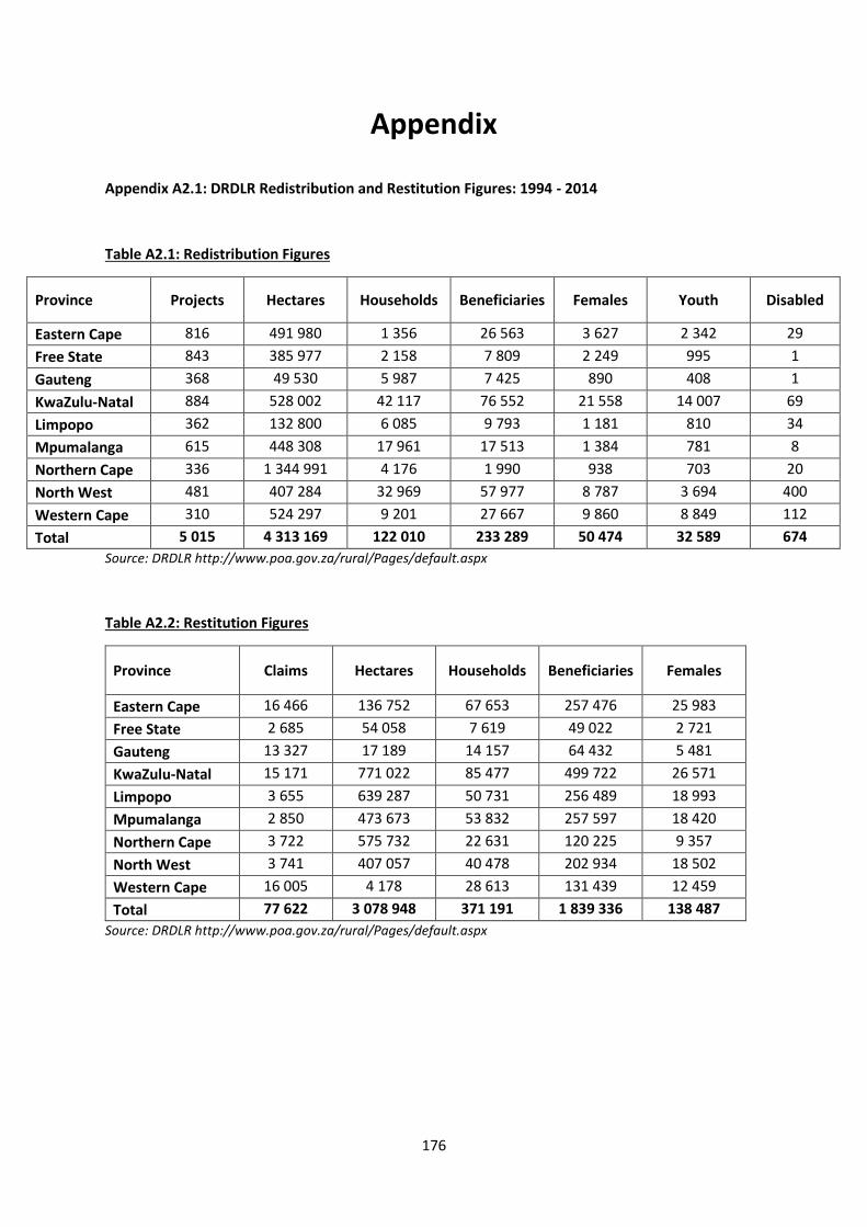
176
Appendix
Appendix A2.1: DRDLR Redistribution and Restitution Figures: 1994 - 2014
Table A2.1: Redistribution Figures
Province Projects Hectares Households Beneficiaries Females Youth Disabled
Eastern Cape 816 491 980 1 356 26 563 3 627 2 342 29
Free State 843 385 977 2 158 7 809 2 249 995 1
Gauteng 368 49 530 5 987 7 425 890 408 1
KwaZulu-Natal 884 528 002 42 117 76 552 21 558 14 007 69
Limpopo 362 132 800 6 085 9 793 1 181 810 34
Mpumalanga 615 448 308 17 961 17 513 1 384 781 8
Northern Cape 336 1 344 991 4 176 1 990 938 703 20
North West 481 407 284 32 969 57 977 8 787 3 694 400
Western Cape 310 524 297 9 201 27 667 9 860 8 849 112
Total 5 015 4 313 169 122 010 233 289 50 474 32 589 674
Source: DRDLR http://www.poa.gov.za/rural/Pages/default.aspx
Table A2.2: Restitution Figures
Province Claims Hectares Households Beneficiaries Females
Eastern Cape 16 466 136 752 67 653 257 476 25 983
Free State 2 685 54 058 7 619 49 022 2 721
Gauteng 13 327 17 189 14 157 64 432 5 481
KwaZulu-Natal 15 171 771 022 85 477 499 722 26 571
Limpopo 3 655 639 287 50 731 256 489 18 993
Mpumalanga 2 850 473 673 53 832 257 597 18 420
Northern Cape 3 722 575 732 22 631 120 225 9 357
North West 3 741 407 057 40 478 202 934 18 502
Western Cape 16 005 4 178 28 613 131 439 12 459
Total 77 622 3 078 948 371 191 1 839 336 138 487
Source: DRDLR http://www.poa.gov.za/rural/Pages/default.aspx
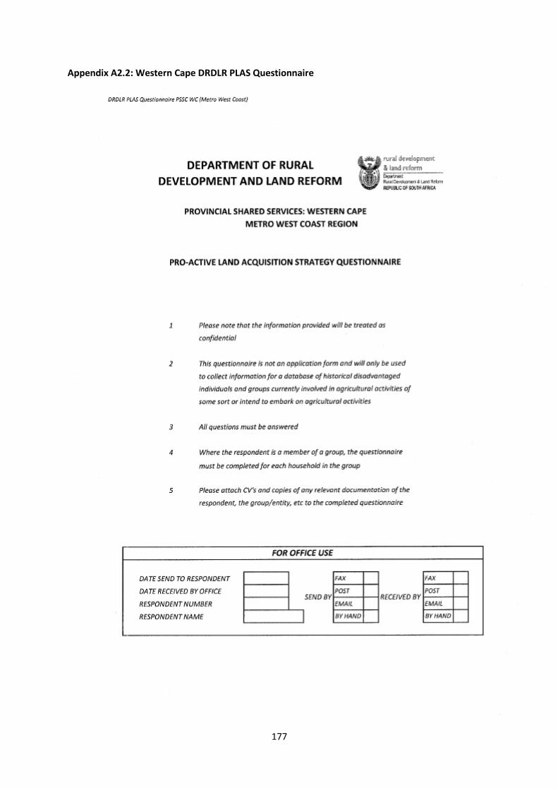
177
Appendix A2.2: Western Cape DRDLR PLAS Questionnaire
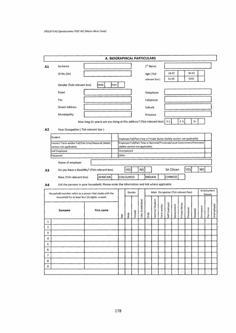
178
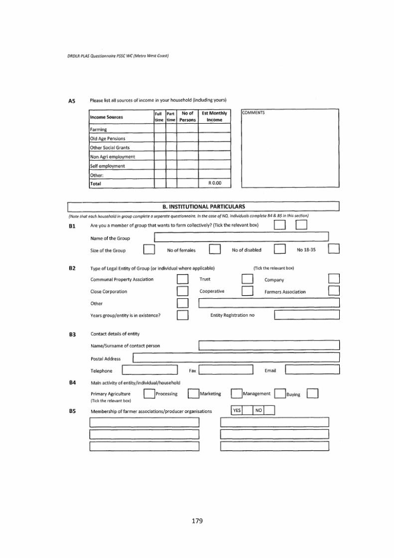
179
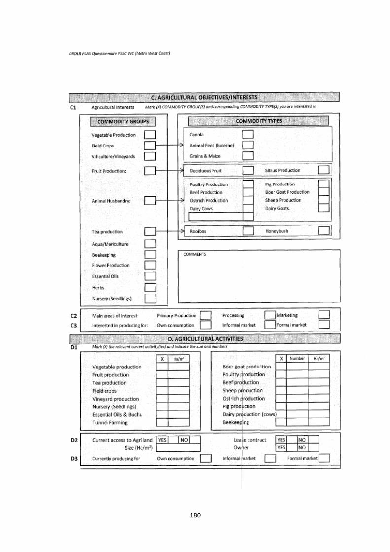
180
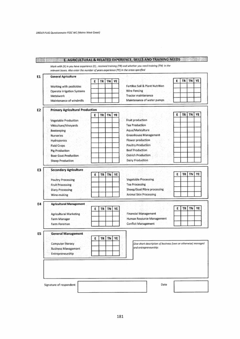
181
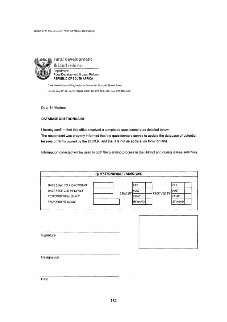
182
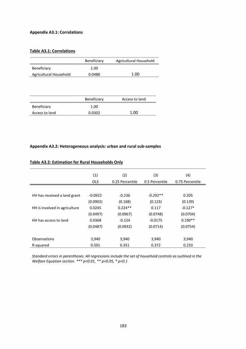
183
Appendix A3.1: Correlations
Table A3.1: Correlations
Beneficiary Agricultural Household
Beneficiary 1.00 Agricultural Household 0.0488 1.00
Beneficiary Access to land
Beneficiary 1.00 Access to land 0.0302 1.00
Appendix A3.2: Heterogeneous analysis: urban and rural sub-samples
Table A3.2: Estimation for Rural Households Only
(1) (2) (3) (4)
OLS 0.25 Percentile 0.5 Percentile 0.75 Percentile
HH has received a land grant -0.0922 -0.236 -0.292** 0.205
(0.0902) (0.168) (0.123) (0.139)
HH is involved in agriculture 0.0245 0.224** 0.117 -0.127*
(0.0497) (0.0967) (0.0748) (0.0704)
HH has access to land 0.0368 -0.124 -0.0175 0.190**
(0.0487) (0.0932) (0.0714) (0.0754)
Observations 3,940 3,940 3,940 3,940
R-squared 0.501 0.351 0.372 0.233
Standard errors in parentheses. All regressions include the set of household controls as outlined in the Welfare Equation section. *** p<0.01, ** p<0.05, * p<0.1
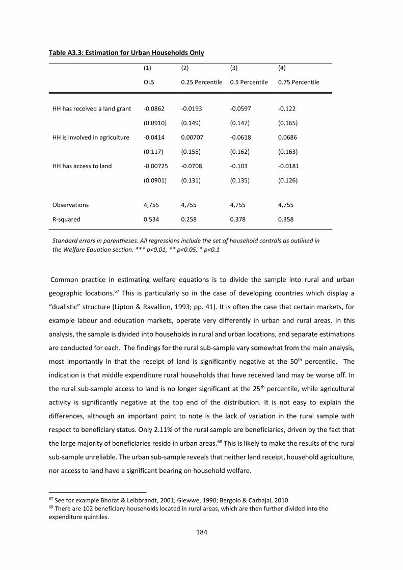
184
Table A3.3: Estimation for Urban Households Only
(1) (2) (3) (4)
OLS 0.25 Percentile 0.5 Percentile 0.75 Percentile
HH has received a land grant -0.0862 -0.0193 -0.0597 -0.122
(0.0910) (0.149) (0.147) (0.165)
HH is involved in agriculture -0.0414 0.00707 -0.0618 0.0686
(0.117) (0.155) (0.162) (0.163)
HH has access to land -0.00725 -0.0708 -0.103 -0.0181
(0.0901) (0.131) (0.135) (0.126)
Observations 4,755 4,755 4,755 4,755
R-squared 0.534 0.258 0.378 0.358
Standard errors in parentheses. All regressions include the set of household controls as outlined in
the Welfare Equation section. *** p<0.01, ** p<0.05, * p<0.1
Common practice in estimating welfare equations is to divide the sample into rural and urban
geographic locations.67 This is particularly so in the case of developing countries which display a
“dualistic” structure (Lipton & Ravallion, 1993; pp. 41). It is often the case that certain markets, for
example labour and education markets, operate very differently in urban and rural areas. In this
analysis, the sample is divided into households in rural and urban locations, and separate estimations
are conducted for each. The findings for the rural sub-sample vary somewhat from the main analysis,
most importantly in that the receipt of land is significantly negative at the 50th percentile. The
indication is that middle expenditure rural households that have received land may be worse off. In
the rural sub-sample access to land is no longer significant at the 25th percentile, while agricultural
activity is significantly negative at the top end of the distribution. It is not easy to explain the
differences, although an important point to note is the lack of variation in the rural sample with
respect to beneficiary status. Only 2.11% of the rural sample are beneficiaries, driven by the fact that
the large majority of beneficiaries reside in urban areas.68 This is likely to make the results of the rural
sub-sample unreliable. The urban sub-sample reveals that neither land receipt, household agriculture,
nor access to land have a significant bearing on household welfare.
67 See for example Bhorat & Leibbrandt, 2001; Glewwe, 1990; Bergolo & Carbajal, 2010. 68 There are 102 beneficiary households located in rural areas, which are then further divided into the expenditure quintiles.
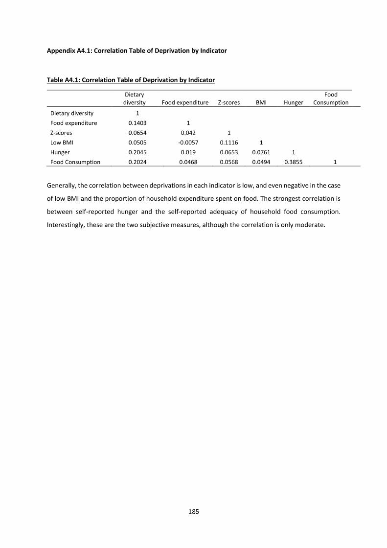
185
Appendix A4.1: Correlation Table of Deprivation by Indicator
Table A4.1: Correlation Table of Deprivation by Indicator
Dietary
diversity Food expenditure Z-scores BMI Hunger Food
Consumption
Dietary diversity 1
Food expenditure 0.1403 1
Z-scores 0.0654 0.042 1
Low BMI 0.0505 -0.0057 0.1116 1
Hunger 0.2045 0.019 0.0653 0.0761 1 Food Consumption 0.2024 0.0468 0.0568 0.0494 0.3855 1
Generally, the correlation between deprivations in each indicator is low, and even negative in the case
of low BMI and the proportion of household expenditure spent on food. The strongest correlation is
between self-reported hunger and the self-reported adequacy of household food consumption.
Interestingly, these are the two subjective measures, although the correlation is only moderate.
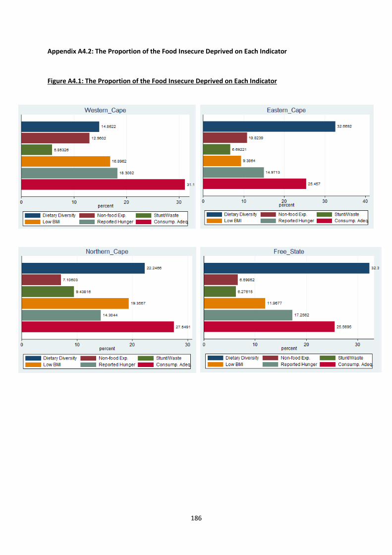
186
Appendix A4.2: The Proportion of the Food Insecure Deprived on Each Indicator
Figure A4.1: The Proportion of the Food Insecure Deprived on Each Indicator
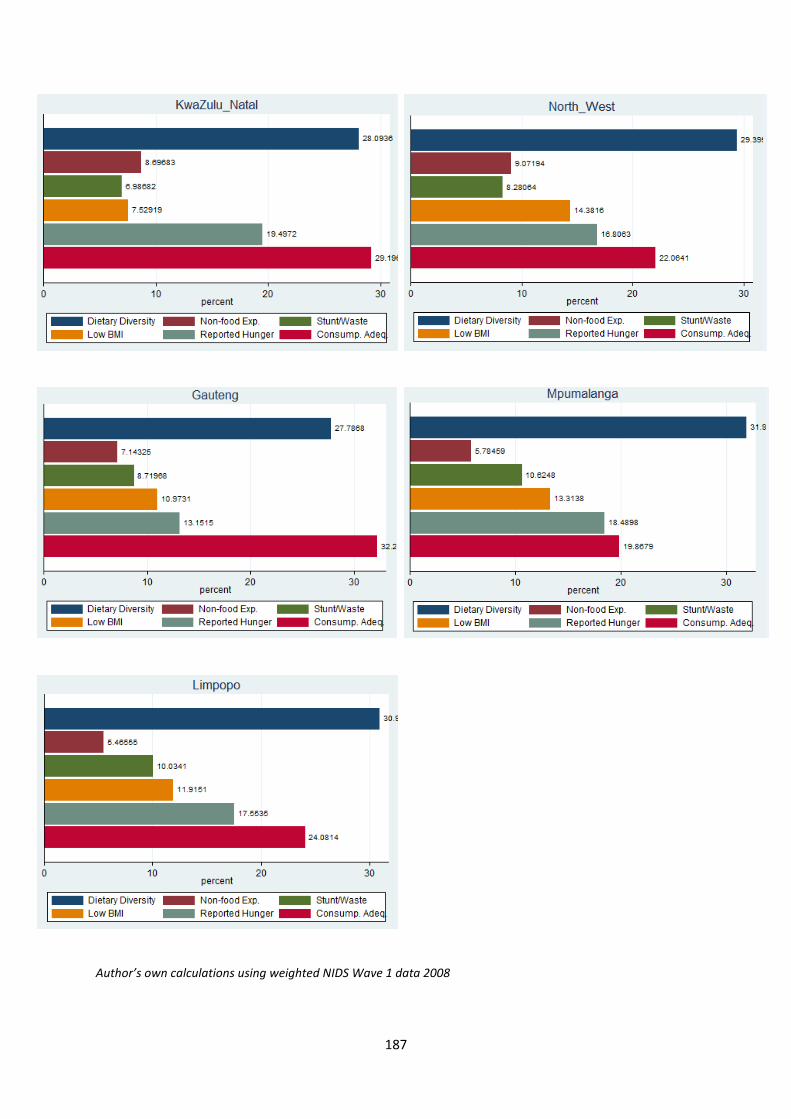
187
Author’s own calculations using weighted NIDS Wave 1 data 2008
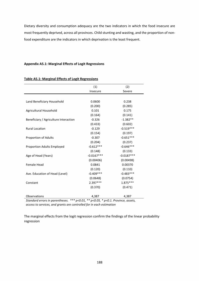
188
Dietary diversity and consumption adequacy are the two indicators in which the food insecure are
most frequently deprived, across all provinces. Child stunting and wasting, and the proportion of non-
food expenditure are the indicators in which deprivation is the least frequent.
Appendix A5.1: Marginal Effects of Logit Regressions
Table A5.1: Marginal Effects of Logit Regressions
(1) (2)
Insecure Severe
Land Beneficiary Household 0.0600 0.238
(0.200) (0.285)
Agricultural Household 0.101 0.175
(0.164) (0.141)
Beneficiary / Agriculture Interaction -0.326 -1.382**
(0.433) (0.602)
Rural Location -0.129 -0.519***
(0.154) (0.197)
Proportion of Adults -0.307 -0.651***
(0.204) (0.237)
Proportion Adults Employed -0.612*** -0.646***
(0.148) (0.133)
Age of Head (Years) -0.0167*** -0.0187***
(0.00406) (0.00498)
Female Head 0.0841 0.00370
(0.120) (0.110)
Ave. Education of Head (Level) -0.409*** -0.483***
(0.0648) (0.0754)
Constant 2.397*** 1.875***
(0.370) (0.471)
Observations 4,387 4,387
Standard errors in parentheses. *** p<0.01, ** p<0.05, * p<0.1. Province, assets, access to services, and grants are controlled for in each estimation
The marginal effects from the logit regression confirm the findings of the linear probability
regression
189
Appendix A6.1: Experiment material
Instructions: Workers
• The results from the tasks you complete today will be used in a research study. It is therefore
important that you carefully read and follow all instructions.
• There are 2 different assignments, with a total of 8 tasks for you to complete.
• You can work on the tasks in any order
• You will have a total of 10 minutes to complete as many of the tasks as you can. You might
not complete all of them.
• We will go through the instructions together and you will be told when you may begin the
tasks.
• The amount you earn may be determined by how productive you are on the tasks.
• The amount you are paid is part of this research and will be determined by an anonymous
third party.
• Your pay can range from R20 to R120: R20 for showing up, and you can earn an additional
amount ranging from R0 to R100 depending on the actions you and the third party take.
• Payment will take place on 20 October 2015, and you will be told how this will work after you
have completed the tasks.
• Everything you do in this study is anonymous.
• There are no tricks in this research. Everything is exactly as it has been described to you.
Instructions for the assignments:
Assignment 1:
• In this assignment you are asked to work on a recognition task.
• On the top of the grid you will be shown a 3-digit code that you must find and check off (with
a cross) from a grid of 3-digit codes in random order.
• The assigned code will appear multiple times in the same grid.
• You will be given 1 point for each correct marking, and you will be subtracted 1 point if you
check off a wrong code. You will not lose any points for failing to check off all occurrences of
the correct code.

190
Below is a simplified example to make sure you understand the assignment:
Assignment 2:
• In this assignment you are asked to work on a set of word scramble problems.
• You must unscramble the words on the left, writing the correct English word in the space
provided.
• The words are grouped into categories to help you.
• You will receive 1 point for each correct answer, and 1 point will be subtracted for each
incorrect answer. No points will be deducted or awarded if you leave an answer blank.
Below is a simplified example to make sure you understand the assignment:
Category: Nouns
Question Answer
1 ODOR DOOR
2 ITYC CITY
3 SKDE DESK
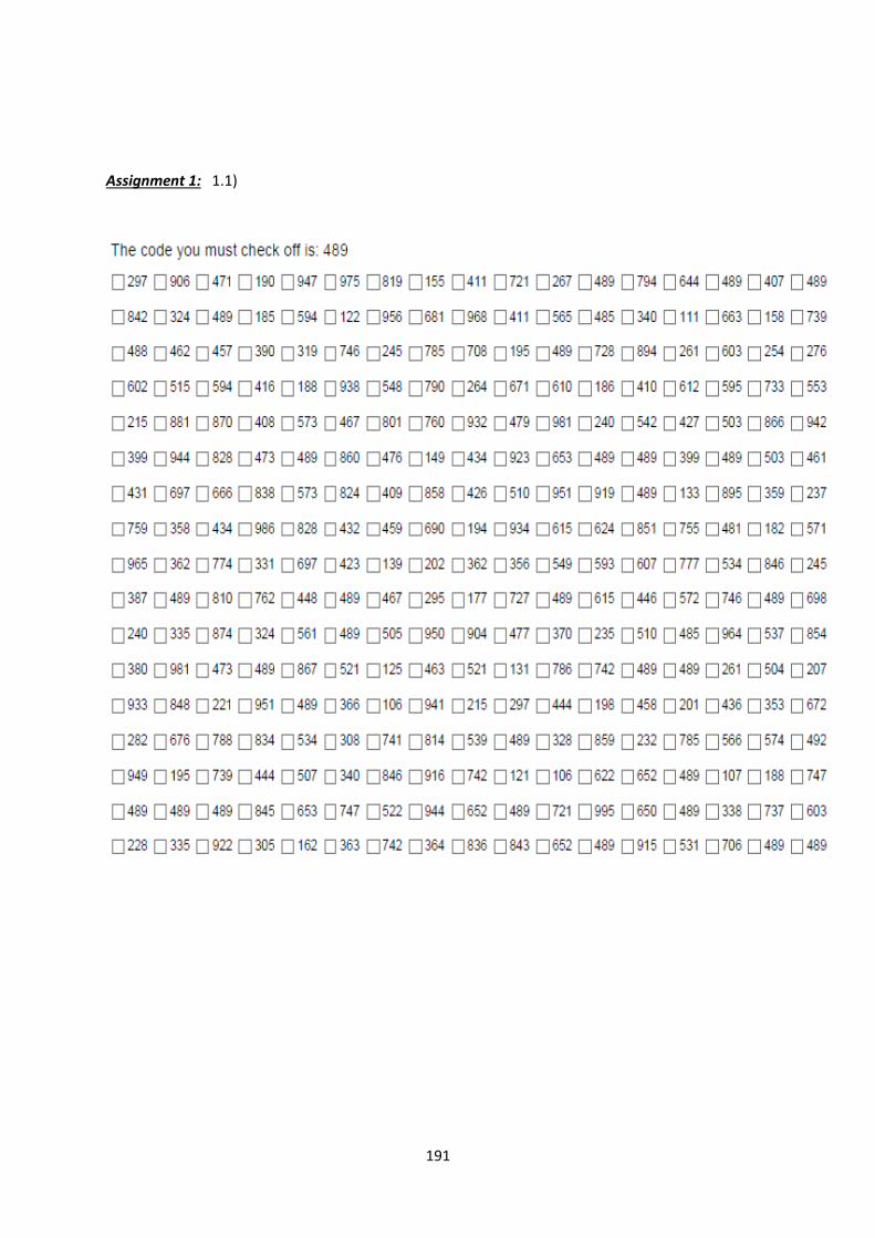
191
Assignment 1: 1.1)
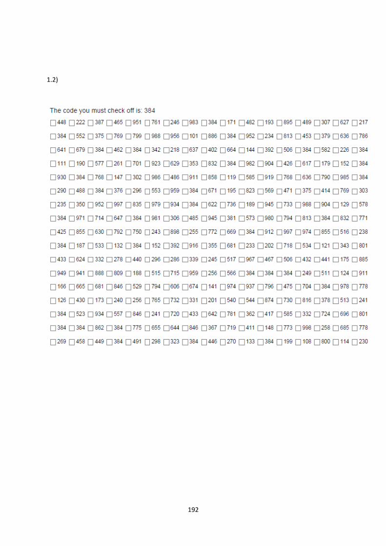
192
1.2)
193
1.3)
194
1. 4)
195
Assignment 2:
2.1) Category: Numbers
Question Answer
1 NWTYTE
2 GIETH
3 RTTYHI
4 EFVI
5 VNEES
6 ETN
7 EINN
8 TSYXI
9 TFYIF
10 OTW
196
2.2) Category: Animals
Question Answer
1 CTA
2 IBDR
3 WOC
4 PEA
5 KARSH
6 SFHI
7 EHROS
8 UOMES
9 NMYOKE
10 ZAERB
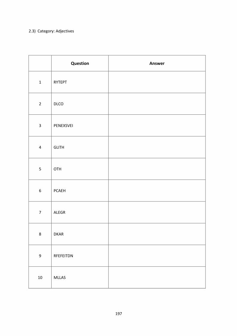
197
2.3) Category: Adjectives
Question Answer
1 RYTEPT
2 DLCO
3 PENEXSVEI
4 GLITH
5 OTH
6 PCAEH
7 ALEGR
8 DKAR
9 RFEFEITDN
10 MLLAS
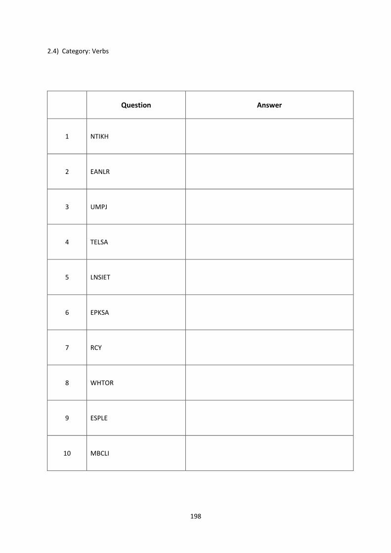
198
2.4) Category: Verbs
Question Answer
1 NTIKH
2 EANLR
3 UMPJ
4 TELSA
5 LNSIET
6 EPKSA
7 RCY
8 WHTOR
9 ESPLE
10 MBCLI
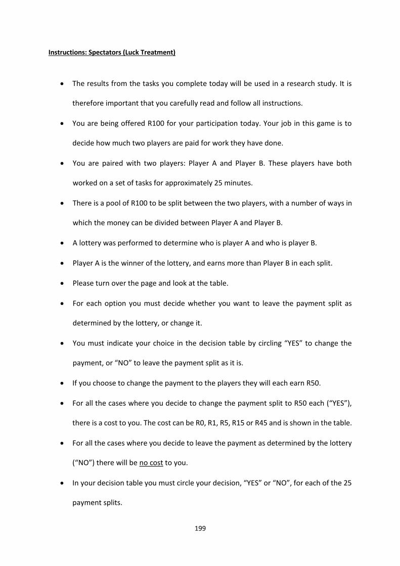
199
Instructions: Spectators (Luck Treatment)
• The results from the tasks you complete today will be used in a research study. It is
therefore important that you carefully read and follow all instructions.
• You are being offered R100 for your participation today. Your job in this game is to
decide how much two players are paid for work they have done.
• You are paired with two players: Player A and Player B. These players have both
worked on a set of tasks for approximately 25 minutes.
• There is a pool of R100 to be split between the two players, with a number of ways in
which the money can be divided between Player A and Player B.
• A lottery was performed to determine who is player A and who is player B.
• Player A is the winner of the lottery, and earns more than Player B in each split.
• Please turn over the page and look at the table.
• For each option you must decide whether you want to leave the payment split as
determined by the lottery, or change it.
• You must indicate your choice in the decision table by circling “YES” to change the
payment, or “NO” to leave the payment split as it is.
• If you choose to change the payment to the players they will each earn R50.
• For all the cases where you decide to change the payment split to R50 each (“YES”),
there is a cost to you. The cost can be R0, R1, R5, R15 or R45 and is shown in the table.
• For all the cases where you decide to leave the payment as determined by the lottery
(“NO”) there will be no cost to you.
• In your decision table you must circle your decision, “YES” or “NO”, for each of the 25
payment splits.
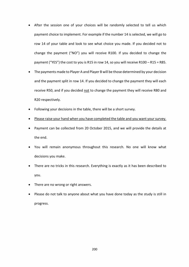
200
• After the session one of your choices will be randomly selected to tell us which
payment choice to implement. For example if the number 14 is selected, we will go to
row 14 of your table and look to see what choice you made. If you decided not to
change the payment (“NO”) you will receive R100. If you decided to change the
payment (“YES”) the cost to you is R15 in row 14, so you will receive R100 – R15 = R85.
• The payments made to Player A and Player B will be those determined by your decision
and the payment split in row 14. If you decided to change the payment they will each
receive R50, and if you decided not to change the payment they will receive R80 and
R20 respectively.
• Following your decisions in the table, there will be a short survey.
• Please raise your hand when you have completed the table and you want your survey.
• Payment can be collected from 20 October 2015, and we will provide the details at
the end.
• You will remain anonymous throughout this research. No one will know what
decisions you make.
• There are no tricks in this research. Everything is exactly as it has been described to
you.
• There are no wrong or right answers.
• Please do not talk to anyone about what you have done today as the study is still in
progress.
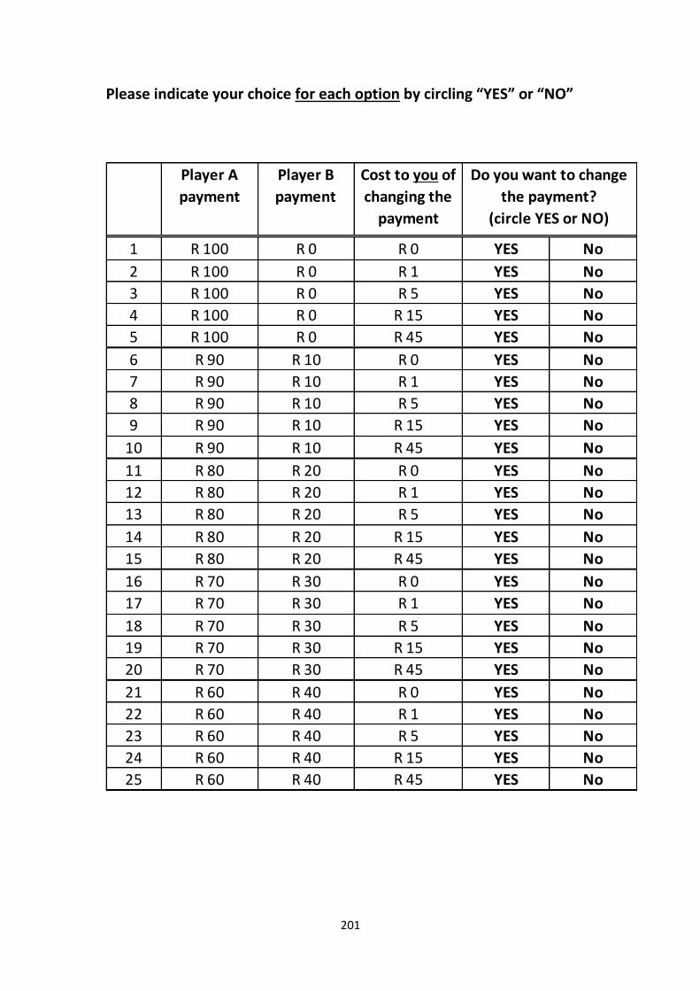
201
Please indicate your choice for each option by circling “YES” or “NO”
1 R 100 R 0 R 0 YES No
2 R 100 R 0 R 1 YES No
3 R 100 R 0 R 5 YES No
4 R 100 R 0 R 15 YES No
5 R 100 R 0 R 45 YES No
6 R 90 R 10 R 0 YES No
7 R 90 R 10 R 1 YES No
8 R 90 R 10 R 5 YES No
9 R 90 R 10 R 15 YES No
10 R 90 R 10 R 45 YES No
11 R 80 R 20 R 0 YES No
12 R 80 R 20 R 1 YES No
13 R 80 R 20 R 5 YES No
14 R 80 R 20 R 15 YES No
15 R 80 R 20 R 45 YES No
16 R 70 R 30 R 0 YES No
17 R 70 R 30 R 1 YES No
18 R 70 R 30 R 5 YES No
19 R 70 R 30 R 15 YES No
20 R 70 R 30 R 45 YES No
21 R 60 R 40 R 0 YES No
22 R 60 R 40 R 1 YES No
23 R 60 R 40 R 5 YES No
24 R 60 R 40 R 15 YES No
25 R 60 R 40 R 45 YES No
Player B
payment
Player A
payment
Cost to you of
changing the
payment
Do you want to change
the payment?
(circle YES or NO)

202
Survey Questions
Q1 What is your gender? Male
Female
Q2 What population group would
you describe yourself as belonging to?
African
Coloured
Asian/Indian
White
other
Refused
Q3 How old are you (in years)
Q4 What is your mother's highest
education level completed? No schooling
Primary school
High school without matric
High school with matric
Tertiary education
Do not know
Q5 What is your father's highest
education level completed? No schooling
Primary school
High school without matric
High school with matric
Tertiary education
Do not know
Q6 In which faculty are you
registered? Commerce
Humanities
Sciences
Engineering & the built environment
Law
Graduate School of Business
Health sciences
Q7 Have you received or are you
receiving financial aid for your studies?
Yes
No
Do not know
Q8 Are you a South African citizen? Yes
No
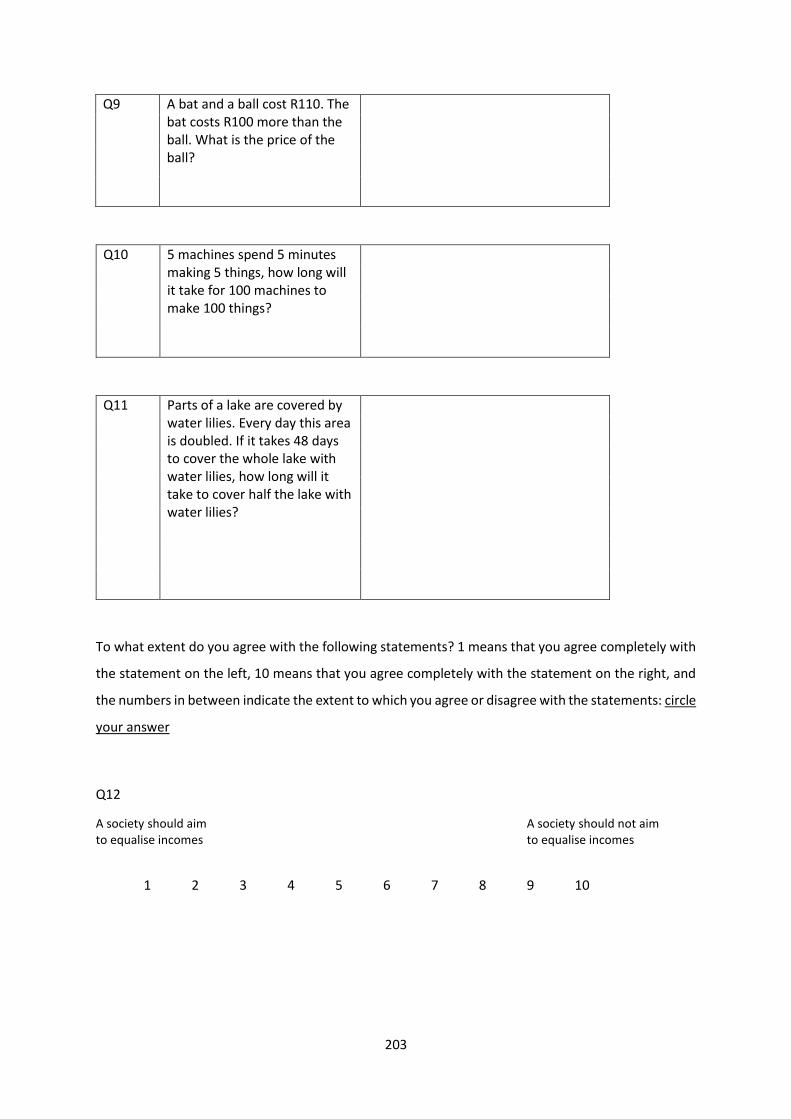
203
Q9 A bat and a ball cost R110. The bat costs R100 more than the ball. What is the price of the ball?
Q10 5 machines spend 5 minutes making 5 things, how long will it take for 100 machines to make 100 things?
Q11 Parts of a lake are covered by water lilies. Every day this area is doubled. If it takes 48 days to cover the whole lake with water lilies, how long will it take to cover half the lake with water lilies?
To what extent do you agree with the following statements? 1 means that you agree completely with
the statement on the left, 10 means that you agree completely with the statement on the right, and
the numbers in between indicate the extent to which you agree or disagree with the statements: circle
your answer
Q12
A society should aim A society should not aim to equalise incomes to equalise incomes
1 2 3 4 5 6 7 8 9 10

204
Q13
In the long run, hard work Hard work doesn’t generally usually brings a better life bring success – it’s more a matter of luck and connections
1 2 3 4 5 6 7 8 9 10
Q14
The government should take People should take more more responsibility to ensure responsibility to provide that everyone is provided for for themselves
1 2 3 4 5 6 7 8 9 10
Q15:
Please explain what motivated your decisions about changing the payment splits or not.
205
References
African Research Institute (ARI). 2013. Waiting for the green revolution land reform in South Africa.
Briefing Note 1301. www.africaresearchinstitute.org Accessed 02/01/2017
Alaba, O. & Chola, L. 2014. Socioeconomic inequalities in adult obesity prevalence in South Africa: a
decomposition analysis. International Journal of Environmental Research and Public Health, 11, pp
3387 – 3406.
Alesina, A. & Angeletos. 2005. Fairness and redistribution. The American Economic Review, 95(4), pp
960 – 980.
Alesina, A. & Giuliano, P. 2009. Preferences for Redistribution. NBER Working Paper 14825.
http://www.nber.org/papers/w14825.pdf Accessed 03/11/2015
Aliber, M. 2009. Exploring Statistics South Africa’s national household surveys as sources of
information about household-level food security. Agrekon, 48(4), pp 384 – 409.
Aliber, M. & Cousins, B. 2013. Livelihoods after Land Reform in South Africa. Journal of Agrarian Change, 13(1), pp 140–165.
Aliber, M., Reitzes, M. & Roefs, M. 2005. Auditing the realisation of democracy and human rights in
the context of rural land reform in South Africa: a component of the METAGORA pilot project: final
technical report. http://www.hsrc.ac.za/en/research-outputs/view/2054 Accessed 09/09/2014
Aliber, M., Reitzes, M., & Roefs, M. 2006. Assessing the alignment of South Africa’s land reform
policy to people’s aspirations and expectations: a policy-oriented report based on a survey in three
provinces. Human Sciences Research Council.
Alkire, S. & Foster, J. 2009. Counting and multidimensional poverty measurement. Oxford Poverty &
Human Development Initiative Working Paper No. 432.
Alkire, S. & Foster, J. 2011. Understandings and misunderstandings of multidimensional poverty
measurement. Oxford Poverty & Human Development Initiative Working Paper No. 43.
206
Alkire, S., Roche, J. M., Santos, M. E., & Seth, S. 2011. Multidimensional poverty index 2011: brief
methodological note. University of Oxford, Department of International Development, Oxford
Poverty and Human Development Initiative, Oxford, UK.
Alkire, S., Foster, J.E., Seth, S., M., Santos, M. E., Roche, & Ballon, P. 2015. Multidimensional poverty
measurement and analysis: chapter 10 – some regression models for AF measures. Oxford Poverty &
Human Development Initiative Working Paper No. 38.
Alkire, S. & Santos, M. E. 2010. Acute multidimensional poverty: a new index for developing
countries. Oxford Poverty & Human Development Initiative Working Paper No. 38.
http://www.ophi.org.uk/wp-content/uploads/ophi-wp38.pdf Accessed 07/10/2014.
Almas, I., Cappelen, A. & Tungodden, B. 2016. Cutthroat capitalism versus cuddly socialism: Are
Americans more meritocratic and efficiency-seeking than Scandinavians? Working paper
Almas, I., Cappelen, A., Sorensen, E. & Tungodden, B. 2010. Fairness and the development of
inequality acceptance. Science, 328(5982), pp 1176-1178.
Altman M., Hart, T. & Jacobs, P. 2009. Food Security in South Africa. HSRC publication, Centre for
Poverty Employment and Growth.
ANC. 1994. The Reconstruction and Development Programme (RDP): A policy framework. pp19 - 20
http://www.sahistory.org.za/sites/default/files/the_reconstruction_and_development_programm_
1994.pdf Accessed 20/06/2016
ANC. 2009. Election manifesto 2009, African National Congress.
http://www.anc.org.za/elections/2009/manifesto/manifesto.html Accessed 15/10/2014
Angrist, J.D. & Pischke, J. 2008. Mostly Harmless Econometrics: An Empiricist’s Companion.
Princeton University Press.
207
Ardington, C. & Case, A. 2009. Health: Analysis of the NIDS Wave 1 Dataset. Discussion Paper no. 2.
http://www.nids.uct.ac.za/publications/discussion-papers/wave-1-papers/93-nids-discussion-paper-
no02/file Accessed 14/10/2014
Assunção, J.J. 2008. Rural Organization and Land Reform in Brazil: The Role of Nonagricultural
Benefits of Landholding. Economic Development and Cultural Change, 56(4), pp 851–870
Atkinson, A. 2003. Multidimensional deprivation: contrasting social welfare and counting
approaches. Journal of Economic Inequality, 1, pp 51 – 65.
Atkinson, A., Cantillion, B., Marlier, E. & Nolan, B. 2002. Social Indicators. The EU and Social
Inclusion. Oxford. Oxford University Press.
http://190.11.224.74:8080/jspui/bitstream/123456789/1151/2/ebooksclub.org__Social_Indicators_
_The_EU_and_Social_Inclusion.pdf Accessed 28/10/2014
Averett, S., Stacey, N and Wang, Y. 2014. Decomposing race and gender differences in underweight
and obesity in South Africa. Economics and Human Biology, 15, pp 23 – 40.
Barr, A. Burns, J., Miller, L. & Shaw, I. 2011. Individual notions of distributive justice and relative
economic status. DFAE-II Working Paper Series, 2011-03.
Barrett C. 2002. Food security and food assistance programs. In Gardner, B.L & Rausser, G.C., editors.
Handbook of Agricultural Economics, 2. Elsevier Science.
Barrett, C. 2010. Measuring food insecurity. Science, 327, pp 825 – 828.
Battersby, J. 2012. Food insecurity amongst urban households. (Book chapter publication
forthcoming by UCT Press/Juta)
Bellu, L.G. 2005. Equivalence scales. Food and Agriculture Organisation of the United Nations.
http://www.fao.org/docs/up/easypol/325/equiv_scales_general_032en.pdf Accessed 11/07/2014
Benoit, K. 2011. Linear regression models with logarithmic transformations. Methodology Institute
London School of Economics. http://www.kenbenoit.net/courses/ME104/logmodels2.pdf Accessed
09/07/2014.
208
Bergolo, M. & Carbajal, F. 2010. Exploring the urban-rural labor income gap in Uruguay: a quantile
regression decomposition. Revista de Analisis Economico, 25(2), pp. 133 – 168.
Bernstein, A., McCarthy, J. & Dagut, S. 2005. Land reform in South Africa: A 21st century perspective.
The Centre for Development and Enterprise: Johannesburg.
Bhorat, H, & Leibbrandt, M. 2001. ‘Modelling vulnerability and low earnings in the South African
Labour Market’, in Bhorat, H., Leibbrandt, M., Maziya, M., van der Berg, S. and Woolard, I., Fighting
poverty, labour markets and inequality in South Africa, UCT Press, Lansdowne, pp 130 – 154.
Binswanger-Mkhize, H.P., Bourguignon, C. & van den Brink, R. 2009. Agricultural Land Redistribution.
Washington, DC: The World Bank.
Bourguignon, F. & Chakravarty, S. 2003. The measurement of multidimensional poverty. Journal of
Economic Inequality, 1, pp 25 – 49.
Bradstock, A. Changing livelihoods and land reform: evidence from the Northern Cape province of
South Africa. World Development, 33(11), pp 1979 – 1992.
Buhmann, B., Rainwater, L., Schmaus, G., and Smeeding, T. 1988. Equivalence scales, well-being,
inequality and poverty: sensitivity estimates across ten countries using the Luxembourg Income
Study (LIS) database. Review of Income and Wealth, 34(2), pp 115 – 142.
Bundy, C. 1988. The Rise and Fall of the South African Peasantry. Cape Town: David Philip
Cappelen, A., Fest, S., Sorenson, E. & Tungodden, B. 2014. The freedom to choose undermines the
willingness to redistribute. Discussion Paper 27/2014, Department of Economics/NHH School of
Economics.
Cappelen, A., Hole, A., Sorenson, E. & Tungodden, B. 2007. The pluralism of fairness ideals: an
experimental approach. American Economic Review, 97(3), pp 818 – 827.
209
Cappelen, A., Konow, J., Sorenson, E. & Tungodden, B. 2013. Just luck: an experimental study of risk
taking and fairness. American Economic Review, 103(4), pp 1398 – 1413.
Cappelen, A., Sorenson, E. & Tungodden, B. 2010. Responsibility for what? Fairness and individual
responsibility. European Economic Review, 54(3), pp 429 – 441.
Centre for Development and Enterprise (CDE). 2005. Land reform in South Africa: a 21st Century
Perspective. Research Report No. 14.
Centre for Development and Enterprise (CDE). 2008. Land reform in South Africa: getting back on
track. Research Report No. 16.
Chinhema, M., Brophy, T., Brown, M., Leibbrandt, M., Mlatsheni C., & Woolard, I. (Eds). 2016.
National Income Dynamics Study Panel User Manual.
http://www.nids.uct.ac.za/documentation/overview-documentation/wave-4 Accessed 02/07/2016
Chitonge, H. & Ntsebeza, L. 2012. Land Reform and Rural Livelihood in South Africa: Does Access to
Land Matter? Review of Agrarian Studies, 2(1), pp 87 – 111.
Choe, C & van Kerm, P. 2014. Foreign workers and the wage distribution: where do they fit in?
CEPS/INSTEAD Working Papers, No. 2014 -02.
Coates, J. 2013. Build it back better: deconstructing food security for improved measurement and
action. Global Food Security, 2, pp 188 – 194.
Coates, J., Frongillo, E., Rogers, B., Webb, P., Wilde, P. & Houser, R. 2006. Commonalities in the
experience and expression of household food insecurity across cultures: what are measures missing?
The Journal of Nutrition, 136, pp 1438S – 1448S.
Coates, J., Swindale, A. & Bilinsky, P. 2007. Household food insecurity access scale (HFIAS) for
measurement of food access: indicator guide. Food and Nutrition Technical Assistance Project.
Washington, D.C.
210
Caballero, B. 2005. A nutrition paradox: underweight and obesity in developing countries. New
England Journal of Medicine, 352(15), pp 1515 – 1516.
Cogill, B. 2003. Anthropometric indicators measurement guide. Food and Nutrition Technical
Assistance Project. Washington, D.C.
Cousins, B. 2013. Land redistribution, populism, and elite capture: new land reform policy proposals
under the microscope. The Journal of the Helen Suzman Foundation, 70. http://hsf.org.za/resource-
centre/focus/focus-70-on-focus/focus-70-oct-b-cousins.pdf/view Accessed 02/01/2017
Cousins, B. 2016. Land reform in South Africa is sinking. Can it be saved? The Nelson Mandela
Foundation. http://www.plaas.org.za/bibliography/land-reform-review-nmf Accessed 02/01/2017
Cousins, B. 2016a. Land reform – the solution to rural poverty? The International Journal for Rural
Development. http://www.rural21.com/english/news/detail/article/land-reform-the-solution-to-
rural-poverty-00002058/ Accessed 02/01/2017
Cousins, B., Hall, R. and Dubb, A. 2014. The Restitution of Land Rights Amendment Act of 2014 -
What are the real implications of reopening land claims? PLAAS Policy Brief 34.
http://www.plaas.org.za/sites/default/files/publications-pdf/Policy%20Brief%2034%20Web.pdf
Accessed 08/11/2016.
Daniels, R., Partridge, A., Kekana, D. & Musundwa, S. Rural Livelihoods in South Africa. Southern
African Labour and Development Research Unit Working Paper Series, No. 122.
Deaton, A. 1997. The Analysis of Household Surveys. The Johns Hopkins University Press: Baltimore
USA.
Deininger, K. 2003. Land Policies for Growth and Poverty Reduction. A World Bank Policy Research
Report, Washington DC.
Department of Agriculture, 2003. Integrated Food Security Strategy for South Africa. Pretoria:
Department of Agriculture.
211
Department of Land Affairs. 1997. White Paper on South African Land Policy.
http://www.dla.gov.za/phocadownload/White-Papers/whitepaperlandreform.pdf
Accessed 08/01/2014
Department of Land Affairs. 2003. Monitoring and evaluating the quality of life of land reform
beneficiaries: 2000/2001. http://www.plaas.org.za/bibliography/me-landreform-beneficiaries-dla
Accessed 10/08/2016
Department of Land Affairs. 2007. Manual for the implementation of the Proactive Land Acquisition
Strategy.
http://www.ruraldevelopment.gov.za/phocadownload/Land_Acquisition_Warehouse/manual%20fo
r%20the%20implementation%20of%20the%20proactive%20land%20acquisition%20strategy.pdf
Accessed 08/05/2014
Department of Planning, Monitoring and Evaluation. 2016. Restitution – setting right the past wrong.
Policy Brief Series.
http://www.dpme.gov.za/keyfocusareas/evaluationsSite/Evaluations/Restitution_Policy%20Brief.pd
f Accessed 16/11/2016
Department of Rural Development and Land Reform. 2012. Settlement and production land
acquisition grant policy framework. http://www.ruraldevelopment.gov.za/tenders/archived-
bids/file/829. Accessed 08/05/2014
Department of Rural Development and Land Reform. 2013. Policy for the Recapitalisation and
Development Programme of the Department of Rural Development and Land Reform.
http://www.ruraldevelopment.gov.za/services/land-reform/recapitalization-and-
development#.U2NndvmSxcE Accessed 08/05/2014
Department of Rural Development and Land Reform. 2016. Annual report 2015/2016.
http://www.drdlr.gov.za/publications/annual-report Accessed 18/11/2016
De Klerk, M., Drimie, S., Aliber, M., Mini, S., Makoena, R., Randela, R., Modiselle, S., Roberts, B.,
Vogel, C., de Swardt, C. & Kirsten, J. 2004. Food security in South Africa: key policy issues for the
medium term. Human Sciences Research Council position paper.
212
de Onis, M., A. Onyango, E. Borghi, A. Siyam, C. Nishida & Siekmann, J. 2007. Development of a WHO
growth reference for school-aged children and adolescents. Bulletin of the World Health
Organization 85: 661-668.
de Swardt, C. 2003. Submission to the parliamentary portfolio committee into a comprehensive
social security system for South Africa. https://pmg.org.za/docs/2003/appendices/030610plaas.pdf
Accessed 07/03/2016
Dinsdale H., Ridler, C. & Ells, L. 2011. A simple guide to classifying body mass index in children.
Oxford: National Obesity Observatory
Durante, R., Putterman, L. & van der Weele, J. 2014. Preferences for redistribution and perception of
Fairness: An experimental study. Journal of the European Economic Association, 12(4), pp 1059 –
1086.
Ermini L. & Hendry, D. 2008. Log income vs. linear income: an application of the encompassing
principle. Oxford Bulletin of Economics and Statistics, 70, Supplement.
Faber, M., & Wenhold, M. 2007. Nutrition in contemporary South Africa. Water SA, 33(3) (Special
Edition); pp 393 - 400
FAO. 2001. FAO’s State of Food Insecurity 2001. Rome: Food and Agriculture Organisation.
Fehr, E. & Schmidt, K. 2001. Theories of fairness and reciprocity – evidence and economic
applications. Prepared for the 8th World Congress of the Econometric Society.
http://papers.ssrn.com/sol3/papers.cfm?abstract_id=255223 Accessed 04.11.2015
Finn, A., Leibbrandt, M. & Woolard, I. 2013. What happened to multidimensional poverty in South
Africa between 1993 and 2010? South Africa Labour and Development Research Unit, Working
Paper Series, Number 99
Firpo, S., Fortin, N., & Lemieux, T. 2007. Unconditional quantile regressions. NBER Technical Working
Paper Series, No. 339.
213
Fleischacker, S. 2005. A Short History of Distributive Justice. Cambridge, MA: Harvard University
Press.
Fortin, N. 2014. Personal correspondence.
Fortin, N., Lemieux, T. & Firpo, S. 2010. Decomposition methods in economics. NBER Working Paper
Series, No. 16045
Foster, J. and Sen, A. 1997. On economic inequality. Enlarged Edition with a Substantial Annexe ‘On
Economic Inequality After a Quarter Century. Clarendon Press, Oxford.
http://graduateeconomist.files.wordpress.com/2012/07/published-1997-on-economic-inequality-
by-amartya-sen.pdf Accessed 28/10/2014
Fournier, J. & Koske, I. 2012. The determinants of earnings inequality – evidence from quantile
regressions. OECD Journal: Economic Studies, 1(1), pp 7 - 36.
Franklin, B., Jones, A., Love, D., Puckett, S., Macklin, J. and White-Means, S. 2012. Exploring
mediators of food insecurity and obesity: a review of recent literature. Journal of Community Health,
37(1), pp 253 – 264.
Glewwe, P. 1991. Investigating the determinants of household welfare in Cote d’Ivoire. Journal of
Development Economics, 35, pp 307 – 337.
Greenberg, S. 2013. The disjunctures of land and agricultural reform in South Africa. Working Paper
26. PLAAS, UWC: Bellville.
Haddad, L., Kennedy, E. & Sullivan, J. 1994. Choice indicators for food security and nutrition
monitoring. Food Policy 19(3), pp 329 – 343.
Hall, R. 2004. Restitution and the politics of land reform: stepping outside the box. Paper presented
at a Conference on Ten Years of Democracy in Southern Africa, Queens University, Kingston, 2-5 May
2004.
214
Hall, R. 2009. Land reform for what use? Land use, production and livelihoods. In Hall, R. (ed)
Another Countryside. Cape Town: Institute for Poverty, Land and Agrarian Studies.
Hall, R. 2010. Reconciling the Past, Present, Future: The Parameters and Practices of Land Restitution
in South Africa. In Walker, Bohlin, Hall and Kepe (eds). Land, Memory, Reconstruction and Justice:
Perspectives on Land Claims in South Africa. Ohio University Press.
Hall, R. 2013. Who, what, where, how, why? Mapping the many disagreements about land and
agrarian reform. Paper presented at the Land Divided Conference, Cape Town, 24 – 27 March 2013
Hall, R. & Cliffe, L. 2009. Introduction in R. Hall and L. Cliffe (eds.). Another Countryside? Policy
Options for Land and Agrarian Reform in South Africa. Institute for Poverty, Land and Agrarian
Studies, Bellville, pp 1–22.
Hart, T. 2009. Food security definitions, measurements, and recent initiatives in South Africa and
Southern Africa. HSRC publication, Centre for Poverty Employment and Growth.
Haughton, J. & Khandker, S. R. 2009. Handbook on Poverty and Inequality. The World Bank
http://siteresources.worldbank.org/INTPA/Resources/429966-
1259774805724/Poverty_Inequality_Handbook_Ch08.pdf Accessed 16/06/2016
Headey, D. & Ecker, O. 2013. Rethinking the measurement of food security: from first principles to
best practice. Food Security, 5(3), pp 327 – 343.
Hendriks, S. 2005. The challenges facing empirical estimation of household food (in)security in South
Africa. Development Southern Africa, 22(1); pp 103 – 123.
Hendriks, S. 2015. The food security continuum: a novel tool for understanding food insecurity as a
range of experiences. Food Security, 7(3), pp 609 – 619.
Hendriks, S., Viljoen, A., Marais, D., Wenhold, F., McIntyre, A., Ngidi, M., van der Merwe, C.,
Annandale, J., Kalaba, M. & Stewart, D. 2016. What can households grow and eat to improve
nutrition in rural communities in South Africa? Research brief
http://www.up.ac.za/media/shared/238/1601-ifnuw-fs-article_-lowres.zp84288.pdf Accessed
02/01/2017
215
Hoddinott, J. & Yohannes, Y. 2002. Dietary diversity as a food security indicator. FCND Discussion
Paper No. 136. International Food Policy Research Institute. Washington, D.C.
Human Sciences Research Council (HSRC), 2004. Food security in South Africa: key policy issues for
the medium term. Position paper. Pretoria: Integrated Rural and Regional Development, HSRC.
Jenkins, S. & Micklewright, J. 2007. New directions in the analysis of inequality and poverty. ISER
Working Paper Series 2007-11.
https://www.iser.essex.ac.uk/research/publications/working-papers/iser/2007-11 Accessed
07/03/2016.
Jonnson, U., Toole, D., 1991. Household Food Security and Nutrition: A Conceptual Analysis. UNICEF,
New York (mimeo).
Jooste, J. 2013. Changing land use patterns in South African with special reference to the Natives
Land Act (1913) and its implications. Parliament of the Republic of South Africa Research Unit
Ker, A. 2011. Conditional and unconditional quantile estimation of telecommunications Engel curves.
Institute for the Advanced Study of Food and Agricultural Policy, Working Paper Series, 11-04.
Kessler, J & Vesterland L. 2015. The external validity of laboratory experiments: qualitative rather
than quantitative effects. In Frechette, G. and Schotter, A. (Eds.) Handbook of Experimental
Economic Methodology. Published online:
http://www.oxfordscholarship.com/view/10.1093/acprof:oso/9780195328325.001.0001/acprof-
9780195328325-chapter-20 Accessed 27.09.2017
Keswell, M. & Carter, M. 2010. Poverty and land redistribution: quasi-experimental evidence from
South Africa’s LRAD programme. Economic Research Southern Africa, Working Paper 190.
http://www.econrsa.org/papers/w_papers/wp190.pdf Accessed 09/09/2014
Kirsten, J., May, J., Hendriks, S., Lyne, M., Machethe, C. & Punt, C. 2003. The Poverty Alleviation and
Food Security Role of Agriculture. The Roles of Agriculture International Conference 20 -22 October.
Rome, Italy.
Koenker, R. and Bassett, G. Regression Quantiles. Econometrica, 46(1), pp 33 – 50.
216
Labadarios, D., Steyn, N.P. and Nel, J. 2011. How diverse is the diet of adult South Africans? Nutrition
Journal 10 (33)
Labadarios, D., Swart, R., Maunder, E.M.W., Kruger, H.S., Gericke, G.J., Kuzwayo, P.M.N., Ntsie, P.R.,
Steyn, N.P., Schloss, I., Dhansay, M.A., Jooste, P., Dannhauser, A., Nel, J.H., Molete, D. & Kotze, T.J.
vW. 2008. Executive summary of the National Food Consumption Survey Fortification Baseline
(NFCS_FB_1) South Africa, 2005. South African Journal of Clinical Nutrition, 21(3) (Suppl), pp 245-
300.
Lahiff, E. 2007. Willing buyer willing seller: South Africa’s failed experiment in market-led agrarian
reform. Third World Quarterly, 28(8), pp 1577 – 1597.
Lahiff, E. 2008. Land reform in South Africa: a status report. Research Report 38. PLAAS, UWC:
Bellville.
Lahiff, E. and Li, G. 2012. Land redistribution in South Africa – a critical review. World Bank working
paper, report number 80874.
http://www.worldbank.org/en/country/southafrica/research/all?qterm=&teratopic_exact=Urban+D
evelopment&docty_exact=Working+Paper Accessed 18/11/2014
Lamont, J. & Favor, C. 2008. Distributive justice. The Stanford Encyclopaedia of Philosophy (Fall 2008
Edition. http://plato.stanford.edu/archives/fall2008/entries/justice-distributive/
Accessed 18/09/2015
Leibbrandt, M. and Woolard, I. 2001. ‘Household incomes, poverty and inequality in a multivariate
framework’, in Bhorat, H., Leibbrandt, M., Maziya, M., van der Berg, S. and Woolard, I., Fighting
poverty, labour markets and inequality in South Africa, UCT Press, Lansdowne, pp 130 – 154.
Leibbrandt, M., Woolard, I., & de Villiers, L. 2009. Technical Paper 1, Methodology: report on NIDS
Wave 1. http://www.nids.uct.ac.za/home/index.php?/Nids- Documentation/technical-papers.html
Accessed 05/01/2012.
217
Levitt, S & List, J. 2007. What do laboratory experiments measuring social preferences reveal about
the real world? Journal of Economic Perspectives, 21(2), pp 153 – 174.
Lipton, M. & Ravallion, M. 1993. Poverty and policy. Policy Research Department, The World Bank
Working Paper Series, WPS 1130.
Madia, T. 2016, November 10. Malema defiant after court appearance: ‘We will take out land, no
matter what’. Mail and Guardian. http://mg.co.za/article/2016-11-07-malema-defiant-after-court-
appearance-we-will-take-our-land-no-matter-how Accessed 04/12/2016
Malik, Vasanti S., Willett, Walter C., & Hu, Frank B. 2013. Global obesity: trends, risk factors and
policy implications. Nature Reviews Endocrinology, 9, pp 13 – 27.
Manuel, T. 2012. Speech: National Planning Commission, on the Presidency Budget Vote debate,
Parliament, 30/05/2012. http://www.polity.org.za/article/sa-manuel-minister-in-the-presidency-
national-planning-commission-on-the-presidency-budget-vote-debate-parliament-30052012-2012-
05-30 Accessed 15/10/2014
Maxwell, D., Coates, J. & Vaitla, B. 2013. How do different indicators of household food security
compare? Empirical evidence from Tigray. Feinstein International Centre, Tufts University: Medford,
USA.
Maxwell, D., Ahiadeke, C., Levin, C., Armar-Klemesu, M., Zakariah, S. & Lamptey, G. 1999. Alternative
food-security indicators: revisiting the frequency and severity of ‘coping strategies’. Food Policy,
24(4), pp 411 – 429.
May, J., Carter, M. & Posel, D. 1995. The composition and persistence of poverty in rural South
Africa: an entitlements approach. Land and Agriculture Policy Centre Paper No. 15. Land and
Agriculture Policy Centre.
Ministry for Agriculture and Land Affairs. 2012. Land redistribution for agricultural development: a
sub-programme of the land redistribution programme.
http://www.ruraldevelopment.gov.za/tenders/archived-bids/file/838. Accessed 03/04/2014
218
National Planning Commission. 2012. An integrated and inclusive rural economy. Chapter Six of the
National Development Plan 2030.
http://www.npconline.co.za/MediaLib/Downloads/Home/Tabs/NDP%202030-CH6-
An%20integrated%20and%20inclusive%20rural%20economy.pdf Accessed 12/09/2013
Ntsebeza, L. 2010. Land and livelihoods in rural South Africa: what prospects for agricultural
activities? Paper presented at the International Conference on “Dynamics of Rural Transformation in
Emerging Economies”, New Delhi, India, April 14 – 16.
O’Laughlin, B., Bernstein, H., Cousins, B. & Peters, P. 2013. Introduction: agrarian change, rural
poverty and land reform in South Africa since 1994. Journal of Agrarian Change, 13(1), pp 1 – 15.
Oxford Poverty and Human Development Initiative (OPHI). 2011. Country Briefing: South Africa.
Multidimensional Poverty Index at a glance. Oxford Department of International Development,
University of Oxford.
Pellicer, M., Piraino, P. & Wegner, E. 2014. Information, mobilization, and demand for redistribution:
a survey experiment in South Africa. A Southern Africa Labour and Development Research Unit
Working Paper Number 139. Cape Town: SALDRU, University of Cape Town.
PLAAS. 2011. Submission to the Department of Rural Development and Land Reform: Comments on
the Green Paper on Land Reform 2011. The Institute for Poverty, Land and Agrarian Studies.
http://www.plaas.org.za/sites/default/files/publications-pdf/PS%2001.pdf Accessed 05/08/2013
Puttergill, C., Bomela, N., Grobbelaar, J., & Moguerane, K. (2011). The limits of land restitution:
livelihoods in three rural communities in South Africa. Development Southern Africa, pp 597-611.
Ranwedzi, N. 2011. The potential and limits of the Proactive Land Acquisition Strategy (PLAS): land
reform implementation in Gauteng Province of South Africa. PLAAS publication:
http://www.plaas.org.za/sites/default/files/publications-pdf/PP%2006.pdf Accessed 18/03/2014
Ravallion, M. 2010. Poverty lines across the world. World Bank Policy Research Working Paper 5284.
219
Rawls, J. 1971. A Theory of Justice. Cambridge, MA: Harvard University Press.
Republic of South Africa. 1996. Constitution of the Republic of South Africa. Accessed 15/10/2014
http://www.gov.za/documents/constitution/1996/96cons2.htm
Republic of South Africa. 2014. Draft Food and Nutrition Security Implementation Plan.
http://www.health-e.org.za/2015/03/05/policy-food-and-nutrition-security-for-the-republic-of-
south-africa/ Accessed 03/12/2015
Rose, D. & Charlton, K.E. 2001. Prevalence of household food poverty in South Africa: results from a
large, nationally representative survey. Public Health Nutrition, 5(3), pp 383-389.
Rose, D. & Charlton, K.E. 2002. Quantitative indicators from a food expenditure survey can be used
to target the food insecure in South Africa. The Journal of Nutrition, 132(11), pp 3235 – 3242.
SA History. 2014. www.sahistory.org.za. Accessed April 2014
Sihlobo, W. & Kapuya, T. 2017. Land policies try to solve imaginary issues at expense of real
problems. Business Day https://www.businesslive.co.za/bd/opinion/2017-06-06-land-policies-try-to-
solve-imaginary-issues-at-expense-of-real-problems/ Accessed 08.10.2017
South Africa Human Rights Commission. 2016. Expropriation Bill pamphlet
http://www.sahrc.org.za/index.php/sahrc-publications/pamphlets Accessed 22/11/2016
Sen, A. 1976. Poverty: an ordinal approach to measurement. Econometrica, 44(2), pp 219 – 231.
Sen, A. 1997. On Economic Inequality. Oxford University Press, New York.
Southern Africa Labour and Development Research Unit. 2014. National Income Dynamics Study
2008, Wave 1. Version 5.2. Cape Town: Southern Africa Labour and Development Research Unit.
Cape Town: DataFirst.
220
State of the Nation Address 2013. President Jacob Zuma.
http://www.info.gov.za/speech/DynamicAction?pageid=461&sid=34250&tid=98676. Accessed
06/03/2013
Statistics South Africa. 2015. Mid-year population estimates. Statistical Release P0302.
Steyn, K., Fourie J, & Temple, N. (eds). 2006. Chronic Diseases of Lifestyle in South Africa 1995 –
2005. Technical Report. Cape Town: South African Medical Research Council.
Swindale, A. & Bilinsky, P. 2006. Household Dietary Diversity Score (HDDS) for Measurement of
Households Food Access: Indicator Guide. Food and Nutrition Technical Assistance Project.
Washington, D.C.
Townsend, M. S., Peerson J., Love, B., Achterberg, C. & Murphy, S. P. 2001. Food insecurity is
positively related to overweight in women. Journal of Nutrition, 131(6), pp 1738 – 1745.
Tsui, Kai-yuen. 2000. Multidimensional poverty indices. Social Choice and Welfare, 19, pp 69 – 93.
United Nations, 2008. Official list of MDG indicators.
mdgs.un.org/unsd/mdg/resources/attach/indicators/officiallist2008.pdf Accessed 23/10/2014
United Nations Development Programme. 2014 Millennium Development Goals Country Report:
South Africa.
http://www.za.undp.org/content/dam/south_africa/docs/Reports/The_Report/MDG_October-
2013.pdf Accessed 23/10/2014
Valente, C. 2009. The food (in)security impact of land redistribution in South Africa: microeconomic
evidence from national data. World Development, 37(9), pp 1540 – 1553.
Walker, C. 2005. The limits to land reform: rethinking ‘the land question’. Journal of South African
Studies, 31(4), pp 805 – 824.
Weideman, M. 2004. Who shaped South Africa’s land reform policy? Politikon, 31(2); pp 219 – 238.
221
Weideman, M. 2006. Land reform, equity and growth in South Africa: a comparative analysis. PhD
thesis. http://wiredspace.wits.ac.za/handle/10539/275 Accessed 10/03/2016.
Wittenberg, M. 2013. NIDS Technical Paper No. 6: a comment on the use of “cluster” corrections in
the context of panel data. http://www.nids.uct.ac.za/publications/technical-papers Accessed
03/07/2016
Wilson, F. 1971. Farming, 1866 – 1966. In Wilson, M. & Thompson L. (eds). The Oxford History of
South Africa. Oxford: Oxford University Press.
Woolard, I. & Leibbrandt, M. 2006. Towards a poverty line for South Africa: background note.
SALDRU
Wooldridge, J. 2006. Introductory econometrics: A modern approach. Mason, OH: Thomson/South-
Western
World Bank (2013). "World Development Indicators 2013." Washington, D.C.: World Bank.
http://data.worldbank.org/data-catalog/world-development-indicators Accessed 12/10/2013
World Health Organisation. 2006. WHO Child Growth Standards: Length/height-for-age, weight-for-
age, weight-for-length, weight-for-height and body mass index-for-age: Methods and development.
Geneva: World Health Organisation.
World Health Organisation. 2015. Obesity and overweight. Fact sheet No 311.
http://www.who.int/mediacentre/factsheets/fs311/en/ Accessed 06/08/2015
Zimmerman, F. 2000. Barriers to participation of the poor in South Africa’s Land Redistribution.
World Development, 28(8), pp 1439 – 1460.