exactly solving packing problems with fragmentation

Exactly solving packing problemswith fragmentation

M. Casazza, A. Ceselli,

Università degli Studi di Milano, Dipartimento di Informatica,

OptLab – Via Bramante 65, 26013 – Crema (CR) – Italy

marco.casazza, [email protected]

April 13, 2015

In packing problems with fragmentation a set of items of known weight is given,together with a set of bins of limited capacity; the task is to find an assignmentof items to bins such that the sum of items assigned to the same bin does notexceed its capacity. As a distinctive feature, items can be split at a price, andfractionally assigned to different bins. Arising in diverse application fields, packingwith fragmentation has been investigated in the literature from both theoretical,modeling, approximation and exact optimization points of view.

We improve the theoretical understanding of the problem, and we introduce newmodels by exploiting only its combinatorial nature. We design new exact solutionalgorithms and heuristics based on these models. We consider also variants fromthe literature arising while including different objective functions and the optionof handling weight overhead after splitting. We present experimental results onboth datasets from the literature and new, more challenging, ones. These showthat our algorithms are both flexible and effective, outperforming by orders ofmagnitude previous approaches from the literature for all the variants considered.By using our algorithms we could also assess the impact of explicitly handlingsplit overhead, in terms of both solutions quality and computing effort.

Keywords: Bin Packing, Item Fragmentation, Mathematical Programming, Branch&Price

1

1 Introduction

Logistics has always been a benchmark for combinatorial optimization methodologies, aspractitioners are traditionally familiar with the competitive advantage granted by optimizedsystems. As an example, Vehicle Routing Problems (VRP) [6] are popular since decades foroperational planning. Indeed, as more problems are understood from a computational point ofview, more details are required to be included in state-of-the art models, driving research fornew solution methods in a virtuous cycle.

The Bin Packing Problem with Item Fragmentation (BPPIF) has been introduced to providesuch an additional level of detail. As in the traditional Bin Packing Problem (BPP), a set ofitems of known weight is given, together with a set of bins of limited capacity; the task is tofind an assignment of items to bins such that the sum of items assigned to the same bin doesnot exceed its capacity. However, unlike in BPPs, items can be split at a price, and fractionallyassigned to different bins.

The BPPIF has first been introduced to model message transmission in community TVnetworks, VLSI circuit design [16] and preemptive scheduling on parallel machines with setuptimes/setup costs. It also proved to suitably model telecommunication optimization, whereitems correspond to data transfer requests, bins correspond to transmission channels, and apacket switching network dimensioning must be carried out [23]. It has also been employed infully optical network planning problems [21]: connection requests are given, that can be splitamong different transmission channels to fully exploit bandwidth, but each split is known tointroduce delays and loss of energy in the transmission process.

The BPPIF arises also as tactical counterpart of the Split Delivery Vehicle Routing Problem(SDVRP) [2], in which the VRP models are enriched by allowing multiple visits to eachcustomer, in order to split its transportation request between multiple vehicles and thus betterexploit vehicle capacities and decrease the routing costs: BPPIF models allow to find optimalfleet sizes.

We also mention that, from a methodological point of view, there is currently a strongconcern in tackling problems in which different kind of decisions need to be taken, some beingcombinatorial while others continuous in nature. It is the case, for instance, of simultaneousrouting and recharge planning of electrical vehicles [20], or rebalancing in bike sharing systems[15]. The BPPIF is one of the most fundamental problems in this family.

From a computational complexity point of view, the BPPIF is NP-Hard, and has beenfirstly tackled in [19]: the authors studied its computational complexity and discussed theapproximation properties of traditional BPP heuristics. In [22] they improved their results,presenting dual asymptotic fully polynomial time approximation schemes that represent the

2

state-of-the-art in approximately solving BPPIFs. Similar models have been introduced in thecontext of memory allocation problems by [5] and considered in [12]: BPPs are presented inwhich items can be split, but each bin can contain at most k item fragments; the theoreticalcomplexity is discussed for different values of k, and simple approximation algorithms are given.Such results have been refined in [11], where the authors provide efficient polynomial-timeapproximation schemes, and consider also dual approximation schemes.

BPPs are in general appealing benchmarks for decomposition and column generation al-gorithms [13]: surveys like [8] contributed to make packing models and algorithms popularin the operations research community. State-of-the-art decomposition algorithms can nowsuccessfully tackle involved BPPs [9, 18]. Indeed, we previously tackled a particular BPPIFin which a fixed number of bins is given, and a solution needs to be found that minimizes thenumber of item fragmentations [4]. We proposed a branch-and-price algorithm that allows tosolve instances with up to 20 items in one hour of computing time.

However, many other BPPIF variants have been discussed in the literature. In fact, forwhat concerns capacity consumption, two versions of the BPPIF can be found: the simplerBPPIF with Size Preserving Fragmentation (BPPSPF), that is the variant described above wheresplitting introduces no overhead, and the BPP with Size Increasing Fragmentation (BPPSIF),in which the weight of each fragment is increased by a certain amount after splitting. Instead,for what concerns the objective of the optimization, the BPPIF arises in the literature in bothfragmentations-minimization form as in [21] and [4], or in bin-minimization form as in [22],in which an upper limit on the total number of fragmentations is imposed, and a solutionminimizing the number of used bins is required. To the best of our knowledge, no exactapproach has been proposed so far for any of these variants.

In this paper we first investigate on further BPPIF properties. These yield compact modelsthat avoid the use of fractional variables. We design both heuristics and new exact algorithmsrelying on these models that (a) are more flexible, as can be applied to all variants of BPPIFdescribed above, including both bin-minimization and fragmentation-minimization objectives,and both size preserving and size increasing variants and (b) are more effective, as when appliedto the variant discussed in [4] are orders of magnitude faster, thus solving in minutes instancesone order of magnitude larger than those of [4]. Exploiting our new tools, we also present acomputational comparison on BPPIF models, assessing the impact of overhead handling onsolution values and computing hardness. Preliminary results were presented in [3].

For the ease of exposition, in Section 2 we consider the bin minimization BPPSPF, itsmathematical programming model and a few theoretical properties on the structure of optimalsolutions, and in Section 3 we detail our new exact algorithm to solve it. Then, in Section 4 wediscuss on how to extend it in order to tackle all the BPPIF variants listed above. In Section

3

5 we present our experimental analysis. Finally, in Section 6 we summarize our results andcollect some brief conclusions.

2 Models

In the following we formalize the bin minimization BPPSPF (bm-BPPSPF). Then, we recalland exploit some properties on the structure of optimal solutions to get an improved formulationthat avoids the use of fractional variables, thus yielding better computational behavior. We alsodiscuss dominance between bounds. To clearly distinguish theorems from the literature by newones, the former are always marked with their reference at the beginning of the claim.

2.1 Mathematical formulation

We are given a set of items I and a set of bins B. Let wi be the weight of each item i ∈ Iand let C be the capacity of each bin. Each item has to be fully packed, but may be split intofragments and fractionally assigned to different bins. The sum of the weights of the (fragmentsof) items packed into a single bin must not exceed the capacity C.

The bm-BPPSPF can be stated as the problem of packing all the items into the minimumnumber of bins by performing at most F fragmentations. It can be formalized as follows:

(BM)

min∑j∈B

uj

s. t.∑j∈B

xij = 1 ∀i ∈ I

∑i∈I

wi · xij ≤ C · uj ∀j ∈ B∑i∈I,j∈B

zij − |I| ≤ F

xij ≤ zij ∀i ∈ I, ∀j ∈ B

0 ≤ xij ≤ 1 ∀i ∈ I, ∀j ∈ B

zij ∈ 0, 1 ∀i ∈ I, ∀j ∈ B

uj ∈ 0, 1 ∀j ∈ B

(2.1)

(2.2)

(2.3)

(2.4)

(2.5)

(2.6)

(2.7)

(2.8)

where each variable xij represents the fraction of item i packed into bin j, each binary variablezij is 1 if any fragment of item i is packed into bin j, and each binary variable uj is 1 if bin jis open.

4

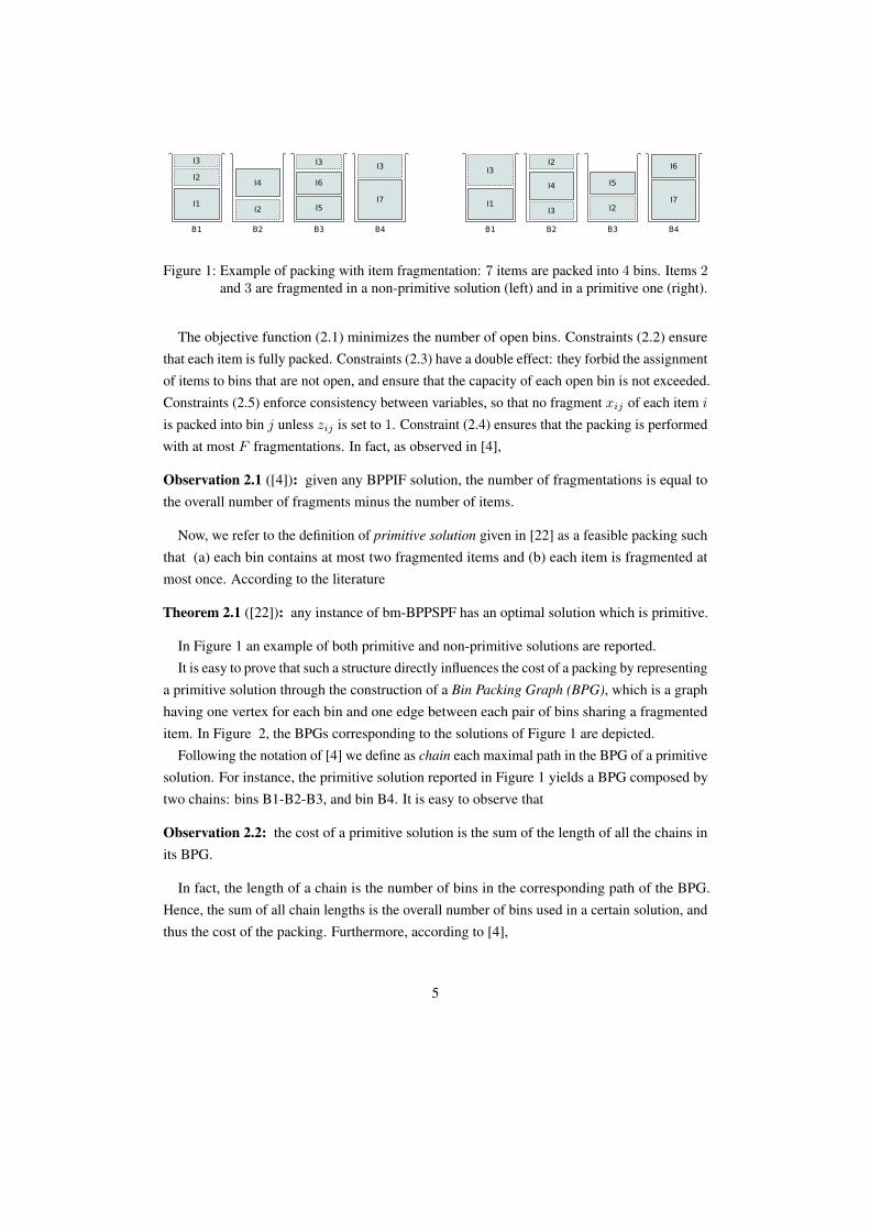
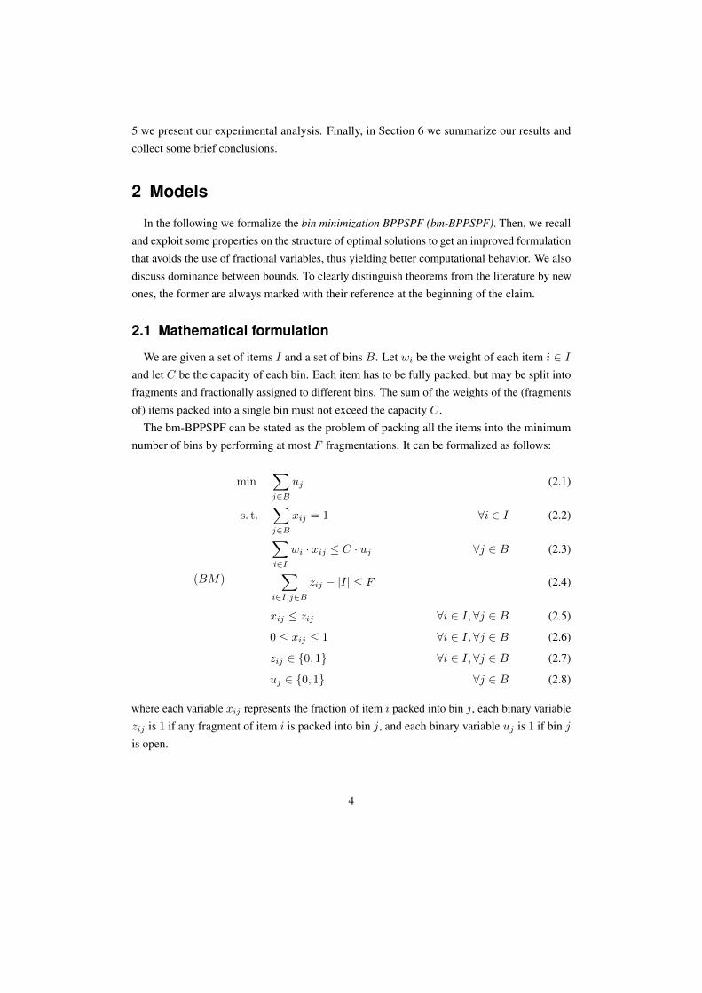
Figure 1: Example of packing with item fragmentation: 7 items are packed into 4 bins. Items 2and 3 are fragmented in a non-primitive solution (left) and in a primitive one (right).

The objective function (2.1) minimizes the number of open bins. Constraints (2.2) ensurethat each item is fully packed. Constraints (2.3) have a double effect: they forbid the assignmentof items to bins that are not open, and ensure that the capacity of each open bin is not exceeded.Constraints (2.5) enforce consistency between variables, so that no fragment xij of each item i

is packed into bin j unless zij is set to 1. Constraint (2.4) ensures that the packing is performedwith at most F fragmentations. In fact, as observed in [4],

Observation 2.1 ([4]): given any BPPIF solution, the number of fragmentations is equal tothe overall number of fragments minus the number of items.

Now, we refer to the definition of primitive solution given in [22] as a feasible packing suchthat (a) each bin contains at most two fragmented items and (b) each item is fragmented atmost once. According to the literature

Theorem 2.1 ([22]): any instance of bm-BPPSPF has an optimal solution which is primitive.

In Figure 1 an example of both primitive and non-primitive solutions are reported.It is easy to prove that such a structure directly influences the cost of a packing by representing

a primitive solution through the construction of a Bin Packing Graph (BPG), which is a graphhaving one vertex for each bin and one edge between each pair of bins sharing a fragmenteditem. In Figure 2, the BPGs corresponding to the solutions of Figure 1 are depicted.

Following the notation of [4] we define as chain each maximal path in the BPG of a primitivesolution. For instance, the primitive solution reported in Figure 1 yields a BPG composed bytwo chains: bins B1-B2-B3, and bin B4. It is easy to observe that

Observation 2.2: the cost of a primitive solution is the sum of the length of all the chains inits BPG.

In fact, the length of a chain is the number of bins in the corresponding path of the BPG.Hence, the sum of all chain lengths is the overall number of bins used in a certain solution, andthus the cost of the packing. Furthermore, according to [4],

5

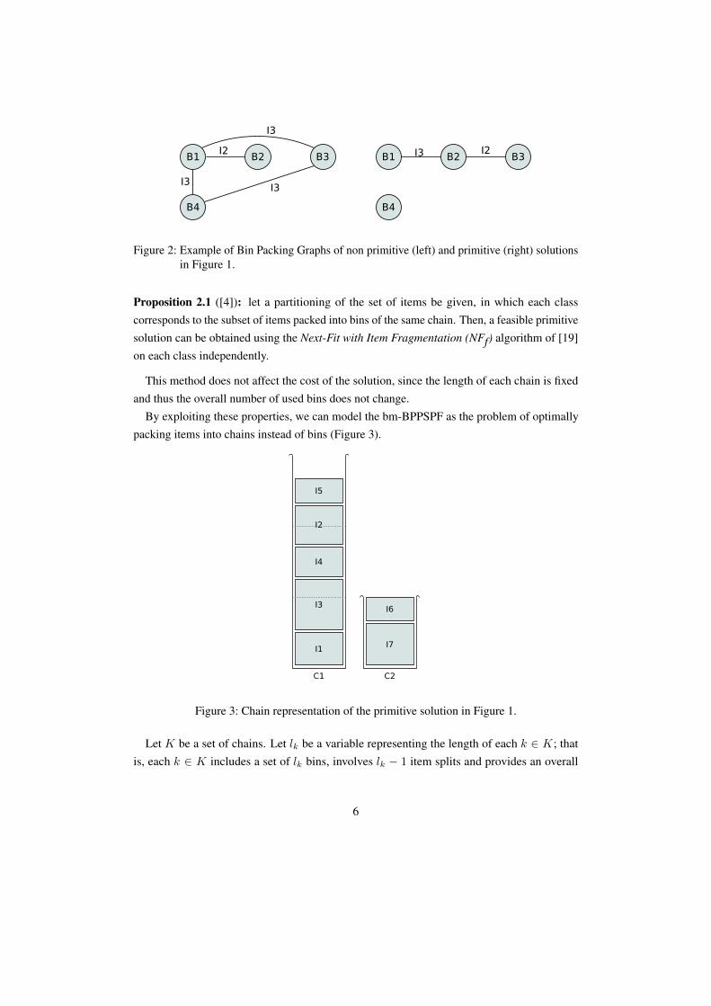
Figure 2: Example of Bin Packing Graphs of non primitive (left) and primitive (right) solutionsin Figure 1.

Proposition 2.1 ([4]): let a partitioning of the set of items be given, in which each classcorresponds to the subset of items packed into bins of the same chain. Then, a feasible primitivesolution can be obtained using the Next-Fit with Item Fragmentation (NFf) algorithm of [19]on each class independently.

This method does not affect the cost of the solution, since the length of each chain is fixedand thus the overall number of used bins does not change.

By exploiting these properties, we can model the bm-BPPSPF as the problem of optimallypacking items into chains instead of bins (Figure 3).

Figure 3: Chain representation of the primitive solution in Figure 1.

Let K be a set of chains. Let lk be a variable representing the length of each k ∈ K; thatis, each k ∈ K includes a set of lk bins, involves lk − 1 item splits and provides an overall

6

capacity of lk · C. Model (2.1) – (2.8) can be reformulated as follows:

(BMC)

min∑k∈K

lk

s. t.∑k∈K

zik = 1 ∀i ∈ I∑k∈K

lk − vk ≤ F∑i∈I

wi · zik ≤ C · lk ∀k ∈ K

vk ≤ lk ∀k ∈ K

zik ∈ B ∀i ∈ I, ∀k ∈ K

lk ∈ N ∀k ∈ K

vk ∈ B ∀k ∈ K

(2.9)

(2.10)

(2.11)

(2.12)

(2.13)

(2.14)

(2.15)

(2.16)

where each binary variable zik is set to 1 if a fragment of item i is packed into chain k, andeach binary variable vk is set to 1 if chain k contains at least one item.

The objective function (2.9) minimizes the number of used bins. Each item can be splitamong bins in the same chain, but no fractional assignment of items to different chains isallowed: constraints (2.10) impose that each item is fully packed in a single chain. Constraints(2.12) ensure that the capacity of each chain is not exceeded, and constraint (2.11) guaranteesthat at most F fragmentations are performed. Constraints (2.13) enforce consistency betweenvariables, so that a chain is used only if its length is at least one.

We remark that a solution of BMC encodes no information on which items are split, noron which items are packed into the same bin of each chain. In fact, due to Proposition 2.1, itis possible to obtain a feasible solution of bm-BPPSPF starting from any feasible solution ofBMC with post processing, by applying the NFf algorithm on each chain independently.

2.2 Extended formulation

From a continuous relaxation point of view, neither formulation (2.1) – (2.8) nor formulation(2.9) – (2.16) offers a significant lower bound: in the first model, it is possible to fix |B| = |I|,and pack each item i into bin j = i fixing each ui = wi/C. The corresponding objectivefunction value would be

∑j uj =

∑i wi/C, yielding a trivial lower bound. Likewise in the

chain model, by fixing |K| = |I| and li = wi/C.Therefore, we propose a reformulation of the problem obtained through Dantzig-Wolfe

7

decomposition [7]. Let zk = (z1k, z2k, . . . , z|I|k) and w = (w1, w2, . . . , w|I|). Let, for each kin K,

Ωk =

(zk, vk, lk) ∈ B|I| × B× N | wT · zk ≤ C · lk ∧ vk ≤ lk

be the set of feasible integer points with respect to constraints (2.12) – (2.16). We relaxintegrality conditions, but replace each Ωk with the convex hull of its Pk extreme integer points

Γk =

(z1k, v

1k, l

1k), . . . , (zPk

k , vPk

k , lPk

k )

and then we impose(zk, uk, lk) =

∑p∈Pk

ypk · (zpk, v

pk, l

pk) (2.17)

with ypk ≥ 0 for each k ∈ K, p ∈ Γk, and∑

p∈Γkypk = 1 for each k ∈ K. That is, each

point is represented as a linear convex combination of points in Γk, and variables y representcoefficients in such a combination.

The model obtained by replacing in the continuous relaxations of formulation BMC thevectors (zk, uk, lk) as indicated in (2.17), and by making explicit the vector indices is

min∑k∈K

∑p∈Γk

ypk · lpk (2.18)

s. t.∑k∈K

∑p∈Γk

ypk · zpik = 1 ∀i ∈ I (2.19)

∑k∈K

∑p∈Γk

ypk · (lpk − v

pk) ≤ F (2.20)

∑p∈Γk

ypk = 1 ∀k ∈ K (2.21)

ypk ≥ 0 ∀k ∈ K, ∀p ∈ Γk (2.22)

Constraints (2.19) can be relaxed in ≥ form, as an optimal solution always exists in whichno item is assigned to bins more than once. Constraints (2.21) can be relaxed in ≤ form byobserving that an empty pattern with lpk = 0, vpk = 0 and zpik = 0 always exists for each k ∈ K;in fact selecting such a pattern is equivalent to setting all the corresponding ypk variables to 0.From this relaxation we also observe that constraint (2.20) can be rewritten as∑

k∈K

∑p∈Γk

ypk · (lpk − 1) ≤ F.

We also observe that since bins are identical, so are the sets Γk. Therefore, we consider a

8

single representative Γ =⋃

k∈K Γk, and aggregate constraints (2.21) as∑p∈Γ

yp ≤ |K|. (2.23)

Furthermore, constraints (2.23) can be removed from the model since it always exists an optimalsolution in which at most |K| patterns are selected. After a rewriting in canonical form, weobtain the following Master Problem (MP):

min∑p∈Γ

yp · lp (2.24)

s. t.∑p∈Γ

yp · zpi ≥ 1 ∀i ∈ I (2.25)

−∑p∈Γ

yp · (lp − 1) ≥ −F (2.26)

yp ≥ 0 ∀p ∈ Γ (2.27)

Observation 2.3: The lower bound provided by the MP dominates that given by the continuousrelaxation of model BMC.

The observation directly follows from the Dantzig-Wolfe decomposition principle. We furtherobserve that, although the continuous relaxations of models BM and BMC are equivalent, theirDantzig-Wolfe decompositions are not. In particular,

Proposition 2.2: the lower bound provided by the MP dominates that obtained throughDantzig-Wolfe decomposition of model BM;

a proof is sketched in subsection 4.1. As discussed in Section 5, we found the lower boundprovided by MP to outperform the other ones also from an experimental point of view.

3 Algorithms

Straightly solving the MP would be impractical, as it would require to consider a tableau with|Γ| columns; therefore, we recur to column generation techniques: we start with a RestrictedMaster Problem (RMP) involving a small subset of columns (see Subsection 3.1), we solveit to optimality, and we use dual information to search for variables having negative reducedcost; to this aim we propose an exact combinatorial algorithm for a particular variant of the 0-1Knapsack Problem (KP) (see Subsection 3.2). If any negative reduced cost variable is found,it is added to the RMP and the column generation process is repeated, otherwise the optimal

9

RMP solution is optimal for the MP as well, and therefore the corresponding value is retainedas a valid lower bound for the bm-BPPSPF. If the final RMP solution is integer, then it is alsooptimal for the bm-BPPSPF; otherwise, in order to find a proven global optimum, we enter asearch tree by performing branching operations (see Subsection 3.4) .

3.1 Initialization

In order to reduce heading-in effects, we populate the RMP with two sets of columns. Thefirst one consists of chains of different length that pack all the items; as a side effect, thisensures the starting RMP to be feasible. The second one is composed by polynomial familiesof dual cuts; as a side effect, they help to prevent stability issues and to speedup the overallcolumn generation process.

Subset-Sum columns Our heuristic initialization approach is based on the iterative gen-eration of columns obtained by solving Subset-Sum problems: the algorithm (see Pseudocode3.1) generates at each iteration a set of chains having the same length, and packs the items byminimizing the residual capacity of each chain. The starting length of the chains is set to one,while the maximum allowed length is set to F .

The packing relies on a Subset-Sum (SS) Procedure that takes in input a set of items J , theirweights w and a capacity Q, and returns the set of items J ⊆ J of largest overall weight notexceeding Q.

function INITRMP(I, w,K,C)for k = 1 . . . F do

J ← Ido

J ←SS(J,w, k · C)add J to RMP as a new columnJ ← J \ J

while J 6= ∅end for

end function

Pseudocode 3.1: RMP initialization alorithm

In our algorithm, the SS Procedure exploits a simple dynamic programming recursion, asdescribed in [17]. It is easy to observe that this approach always produces a set of columnsforming a feasible RMP solution. In particular, during iteration k = 1, the initializationalgorithm packs all the items in chains of single bins, thereby creating a BPPSPF solution withno fragmentations.

10

Dual cuts for BPPSPF Then we restrict the dual space of the MP, in order to obtainoptimal MP solutions faster. We exploit a variant of the family of dual cuts proposed in [24]for the Cutting-Stock Problem. Let λ and µ be the vector of non negative dual variablescorresponding to constraints (2.19) and (2.20), respectively. We formulate the following

Proposition 3.1: for each pair of subsets S and T of I such that∑

i∈S wi ≤∑

i∈T wi, nooptimal dual solution violates the following inequalities∑

i∈Sλi ≤

∑i∈T

λi (3.1)

In fact, if any such inequality were violated, all basic columns of the MP representing chainsincluding T can be replaced by columns where items in T are removed and replaced by itemsin S, as these still encode feasible chains. The reduced cost of these new columns would benegative, thus contradicting the optimality of the solution.

Intuitively, these inequalities encode the following condition: an optimal solution alwaysexists, in which subsets of small size yield less dual contribution to the reduced costs. Moreover,the linear combination of dual cuts (3.1) and columns in the RMP, gives origin to new patternsthat may avoid the generation of further columns.

From an implementation point of view, each dual cut is represented by a column p in whichzpi = 1 for each i ∈ S and zpi = −1 for each i ∈ T . These valid dual cuts are in exponentialnumber. Very recent contributions showed that in particular cases their dynamic generationis appealing [14]. Instead, we found it useful to focus on sets S and T of small cardinality,considering two cases in which |S| = |T | = 1, and |S| = 2 and |T | = 1, and we add thecorresponding columns to the RMP before the execution of the column generation process.

3.2 Pricing problem

For each p ∈ Γ, the reduced cost of variable yp is computed as

πp = lp −∑i∈I

λi · zpi + µ · (lp − 1).

The pricing problem, that is the problem of finding the most negative reduced cost column,

11

can be stated as follows:

π∗ = minp∈Γ

lp −∑i∈I

λi · zpi + µ · (lp − 1) (3.2)

s. t.∑i∈I

wi · zpi ≤ C · lp

0 ≤ lp − 1 ≤ F

zpi ∈ B ∀i ∈ I

lp ∈ N

Let us state the objective function of the pricing problem (3.2) in maximization form, andcollect the coefficients of terms zpi and lp

π∗ = −maxp∈Γ

∑i∈I

λi · zpi − (µ+ 1) · lp − µ.

That is, λi and (µ+ 1) represent the prize for packing item i and the cost for using each bin inthe current chain, respectively. Therefore, the pricing problem is a variant of the 0-1 KnapsackProblem (KP) [17]. It aims to find an optimal tradeoff between the cost of using bins and theprofit of including items, respecting a single aggregated capacity constraint and an upper boundon the available capacity. We indicate such a variant as the Variable Size KP (VSKP).

To solve the VSKP we develop the following ad-hoc pseudo-polynomial time algorithmbased on the well-known dynamic programming approach for the 0-1 KP [17]: let M(I , c) bethe cost of an optimal VSKP solution in which only items I ⊆ I are allowed to be selected,and exactly c units of capacity are consumed. The values M(I , c) can be recursively computedas follows:

M(I ∪ i, c) = −(µ+ 1) · dc/Ce+

M(I , c), if wi > c

maxM(I , c);M(I , c− wi) + λi

, otherwise

where M(∅, c) = −µ for each 0 ≤ c ≤ F · C. Thus, the final cost of an optimal VSKP is

π∗ = max0≤c≤F ·C

M(I, c)

It is easy to keep track of the subset of items forming an optimal solution by storing whicharguments yield maxima in the above expression. The complexity of the overall procedure isO(F · C · |I|).

As multiple pricing strategy, after preliminary experiments we found out to be beneficial

12

adding |K| columns at each column generation iteration, corresponding to the valuesM(I, k·C)

for k = 1 . . . |K|.

3.3 Primal Heuristics

When the column generation process is over, the optimal MP solution can be fractional. Inthat case we run primal (upper bounding) heuristics: if the upper and lower bounds match,global optimality for the bm-BPPSPF is proved. In order to find good integer solutions quickly,we developed the following Iterative Subset-Sum Heuristic (ISSH), that is built on the SSHheuristic for fragmentations-minimization BPPSPF (fm-BPPSPF) proposed in [4]. The ideais to iteratively fix the number of open bins and pack all the items by solving a fm-BPPSPF,until a feasible solution is reached, that packs all items with a number of fragmentations notexceeding F . The algorithm is detailed in Pseudocode 3.2.

function ISSH(I, w, F,C)B ← d

∑i∈I wi/Ce

loopP, F ← SSH(I,B,w,C)if F ≤ F then

return P,Belse

B ← B + 1end if

end loopend function

Pseudocode 3.2: ISSH heuristic

The ISSH makes use of the SSH procedure [4], that takes as arguments the set of items I ,the number of bins B, the vector of weights w and the capacity C, and returns a set of chainsP and the number of fragmentations F . The algorithm always ends with a feasible solution forthe bm-BPPSPF, since it is always possible to find a feasible packing that uses |I| bins.

Additionally, we considered several general purpose MILP heuristics to be run on MPfractional solutions, that are included in the framework we used in our implementation; moredetails are reported in Section 5.

3.4 Branch and bound

When the optimal MP solution is fractional, and upper and lower bounds do not match, wecheck which integrality constraints are not satisfied, and we explore a search tree by means of

13

branching.In our case, branching is particularly involved, as the MP is prone to symmetries. We devised

the following binary branching rule, in which chains are progressively defined and an integersolution is enforced through the assignment of items to the chains.

Let us suppose that a particular head item is defined for each chain, and that at a certain nodeof the branching tree, items in a set H ⊆ I are selected to be head items of |H| chains. At theroot node, H = ∅; then, recursively, a branching item is either selected to be assigned to oneof the chains identified by an item in H , or becomes a new head item, thereby identifying anadditional chain.

Phase 1 - Item assignment If H = ∅, we directly skip to Phase 2. Otherwise, let yp bethe values of each variable yp in a fractional MP solution and, for each i ∈ I and h ∈ H

tih =∑p∈Γ

zpi · zph · y

p

be a coefficient that indicates how much item i is packed with head item h in the fractionalsolution. We search for an item i and a head item h corresponding to the most fractionalassignment in the current fractional solution, that is

(h, i) ∈ argminh∈H,i∈I

∣∣∣∣tih − 1

2

∣∣∣∣ .If tih is fractional, then we perform binary branching: we enforce i to be always packed with

h in one branch, while we forbid i to be packed with h in the other. If instead tih is integer, weproceed to Phase 2.

Phase 2 - Chain selection If no fractional assignment of items to chains defined by Hcan be found, then it also holds that no column in the MP having a fixed head item is fractionallyselected. In fact, if it were, such fractionally selected columns should be identical, but in ourMP it is never profitable to generate the same column twice. However, it is still possible thatfractional solutions arise due to splitting in additional chains for which no head item is fixed.

We check this condition as follows. We search for the most fractionally selected MP variable,that is we identify

p ∈ argminp∈Γ

∣∣∣∣yp − 1

2

∣∣∣∣ .If yp is integer, then a full integer solution is found: the incumbent is possibly updated and

14

the branching node is fathomed.Otherwise, an arbitrary item i is selected, such that zp

i= 1 and i 6∈ H . Then we add i to the

set H , we initialize Ii = i, and we restart branching from Phase 1.

Pricing implementation Our branching strategy changes the nature of the pricing problem.Let Ih be the set of items forced to be packed with head item h, let Wh =

∑i∈Ih wi be their

sum of weights, and let Ih be the set of items whose packing with h is forbidden. Let I0 be theset of items which are not forced to be packed to any head item, such that

I0 = I \⋃h∈H

Ih.

We deal with additional constraints introduced in both branching phases by solving |H|+ 1

VSKPs. The first VSKP aims at finding the chain without head item yielding the most negativereduced cost:

π0 = − max0≤c≤F ·C

M(I0, c).

Then, we solve a VSKP for each h ∈ H , each searching for the chain with head item h

yielding the most negative reduced cost:

πh = −∑i∈Ih

λi − max0≤c≤F ·C−Wh

M(I0 \ Ih, c).

that is, we solve a VSKP where the available capacity is decreased by the weights of the itemsfixed in Ih, forbidding the selection of items in Ih and decreasing the final reduced cost by thesum of the prizes of the items in Ih.

We experimentally observed that, although the number of VSKP subproblems increasesas the depth of the branching tree increases, the overall number of chains remains limited.Additionally, the solutions of the |H|+ 1 VSKPs yield well diversified columns, that are inturn useful to perform more effective multiple pricing, thus speeding up the column generationprocess.

In particular, after preliminary experiments, we set a different multiple pricing strategy inthe inner nodes of the branching tree. That is, at each iteration of column generation we add tothe RMP (a) one column, corresponding to the packing defining the value of π0 and (b) |H|columns, each corresponding to the packing defining the value of iπh for each h ∈ H , providedthey have negative reduced cost.

15

4 Tackling BPPIF variants

Several BPPIF variants arise in the literature and in practical applications. The main featureschanging among them are the possibility of handling overhead in item weights after each splitand the objective to be optimized.

In the following we first describe how to handle these features in chain based models. Thenwe discuss on how to adapt our algorithms to obtain a unified framework.

4.1 Extending Models

First, still owing to practical applications, packing an item may introduce an overhead inits weight. This is the typical case of transmissions over packed-switching networks, in whichdata are split into packets that need additional headers (and trailers) to be delivered, as stated in[22].

Let ε be a constant representing an amount of overhead, that we suppose to satisfy ε ≤mini∈I wi. The BPPIF with size-increasing fragmentation (BPPSIF) is the variant of BPPIFin which a weight ε is attached to all fragments packed into bins, including those fragmentscorresponding to unfragmented items. We first observe that according to the literature,

Proposition 4.1 ([22]): each solution of bin-minimization BPPSIF has a primitive solution.

Thus we adapt the chain-based BPPIF model BMC (2.9)–(2.16), by changing constraint(2.12) into ∑

i∈I(wi + ε) · zik + ε · (lk − 1) ≤ C · lk ∀k ∈ K, (4.1)

where the term ε · (lk − 1) is the overhead given by the chain fragmentations.A corresponding extended formulation can also be obtained, by performing the reformulation

steps described on (2.18)–(2.22), and changing only the definition of sets Γk. Indeed, ourBPPSPF models can be obtained as a special case of BPPSIF ones by setting ε = 0.

We remark that other overhead policies may be pertinent depending on the practical applica-tion, as in [19]. The methodology may still be valid depending on the existence of a primitiveoptimal solution.

Second, bin-minimization is not the only objective function discussed in the literature. Inparticular BPPIFs arise in applications, in which the number of available bins is fixed, and thenumber of fragmented items has instead to be minimized [21]. Although different policiesmay be considered for penalizing fragmentations, appealing ones turn out to be equivalent. Forinstance, according to [4],

16

Proposition 4.2 ([4]): an optimal solution for the fragmentations minimization BPPIF alwaysexists, that is primitive,

and therefore

Observation 4.1: the problem of minimizing the number of item fragments is equivalent tothat of minimizing the overall number of fragmentations,

as each item is fragmented at most once, and hence the number of fragments is equal to thenumber of items plus the number of fragmentations.

We therefore consider the size preserving fragmentation-minimization BPPIF (fm-BPPSPF)problem modeled in [4]:

(FM)

min∑

i∈I,j∈Bzij − |I|

s. t. 2.2, 2.5, 2.6, 2.7∑i∈I

wi · xij ≤ C ∀j ∈ B

(4.2)

(4.3)

The objective function (4.2) minimizes the number of fragmentations, and equivalently thenumber of fragments. Constraints (4.3) ensure that the capacity of each bin is not exceeded.

In principle, this model is compact and can thus be directly managed by a generic solver.However, according to the experimental results obtained in [4], such an approach fails even onvery small instances. The branch-and-price algorithm of [4] allows to solve about 40% moreinstances than CPLEX, but fails as the size of the instances increases.

Indeed we could obtain substantially better results by adapting the chain based methodsdetailed in the previous section. Still without loss of optimization power, by exploitingProposition 4.2 we consider only primitive solutions, and the corresponding BPG. As before,let lk be the length of any chain k in the BPG, that is in turn the number of fragmentations inthe chain plus one. The fm-BPPSPF can therefore be modeled with a chain formulation, inwhich the objective function is to minimize the overall number of fragmentations:

(FMC)

min∑k∈K

lk − vk

s. t. 2.10, 2.12, 2.13− 2.16∑k∈K

lk ≤ |K|

(4.4)

(4.5)

The objective function (4.4) minimizes the overall number of fragmentations by minimizing

17

the sum of the costs of the chains in the corresponding BPG. Constraints (4.5) ensure that allitems are packed into at most |K| bins.

As the compact models, also the chain model can be directly solved by a generic solver,but as before it is easy to prove that the continuous relaxations of both models FM and FMCdo not offer significant lower bounds. Therefore, we adapt the Dantzig-Wolfe decompositionproposed in Subsection 2.2. In fact, by replacing in the continuous relaxations of formulationFMC the vectors (zk, vk, lk) as indicated in (2.17), and by making explicit the vector indices,we obtain the following formulation:

min∑k∈K

∑p∈Γk

ypk · (lpk − v

pk)

s. t. 2.19, 2.21, 2.22∑k∈K

∑p∈Γk

ypk · lpk ≤ |K|

that after applying the same reformulation steps performed for model (2.18) – (2.22), yields thefollowing:

(F −MP )

min∑p∈Γ

yp · (lp − 1)

s. t. 2.25, 2.27

−∑p∈Γ

yp · lp ≥ −|K|

(4.6)

(4.7)

The objective function (4.6) minimizes the overall cost, given as the sum of fragmentationsperformed in each chain. Constraint (4.7) ensures that items are packed into at most |K| bins.

As far as the quality of bounds is concerned, we can prove the following.

Proposition 4.3: The lower bound given by F-MP dominates that obtained by Dantzig-Wolfedecomposition of model FM.

The latter has been introduced in [4] as a basis for an exact branch-and-price algorithm: itconsists of an extended formulation with one column for each feasible assignment pattern ofitems to bins. Intuitively, given an optimal MP solution yp, we can run NF(f) on each patternp ∈ Γ of length lp, build lp assignment patterns of items to bins, corresponding to the lp binsin the NF(f) solution, and select each of them for a value yp. This solution is feasible for theextended formulation of [4]. Indeed, we experimentally observed it to be often suboptimal,thereby providing weaker bounds.

We remark that model F-MP, including (4.6), (2.25), (2.27) and (4.7), differs from model

18

MP, including (2.24)–(2.27), only for the exchange between the objective function and theconstraint on the available resource: the first model limits the number of bins while minimizingthe number of fragmentations. The second does the opposite. Indeed the dominance proofamong bounds readily extends to bm-BPPIF models.

For completeness, we also mention that

Proposition 4.4: an optimal solution to fm-BPPSIF always exists, that is primitive.

The proof is similar to that of Proposition 4.2, additionally observing that a non-primitiveoptimal solution would just introduce more overhead than a corresponding primitive one.Therefore, a chain-based modeling of fm-BPPSIF can be obtained by combining the stepsdescribed above.

4.2 Extending algorithms

Overhead handing nicely fits in our framework. In fact, Constraint (4.1) can be easilytransposed into the pricing problem and solved as a variant of VSKP in which bins capacity isC = C − ε, and a capacity of ε is set as consumed since the beginning. Due to Constraint (4.1)the weight of each item i is then wi = wi + ε. Once again, when ε = 0, the pricing algorithmis exactly the one described in Section 3.2.

We could successfully adapt our column generation techniques also to fragment-minimizationproblems. In this case, the models differ in the objective function of the pricing problem: let λand µ be respectively the vector of non negative dual variables corresponding to constraints(2.25) and (4.7); the reduced cost of each variable yp is

minp∈Γ

lp − 1−∑i∈I

λi · zpi + µ · lp.

By rewriting the objective function in maximization form, and by collecting the coefficients ofterms zpi and lp, we obtain

max∑i∈I

λi · zpi − (µ+ 1) · lp + 1.

that is still a VSKP, and can therefore be solved as explained in section 3.2.Every other detail of the algorithm remains the same, with the only exception that instead of

using ISSH as primal heuristic, it is more appropriate to directly include SSH as proposed in[4] when optimizing fragmentation-minimization problems.

19

5 Experimental results

We implemented our algorithms in C++, using the framework SCIP [1] version 3.0.2, keepingthe default options but forcing single thread execution. In particular, that includes a full suiteof general purpose primal heuristics. The LP subproblems were solved using the simplexalgorithm implemented in CPLEX 12.4 [10]: the framework automatically switches betweenprimal and dual methods. We refer to our exact branch-and-price algorithm as BPA in theremainder.

As a benchmark we considered the branch-and-cut implemented in CPLEX 12.4, using themathematical programming models described in Section 2 and Section 4, and keeping againdefault settings besides forcing single thread execution. All the tests have been performed on aPC equipped with an Intel(R) Core2 Duo CPU E6850 at 3.00 GHz and 4 GB of memory.

As a first check, we tested our BPA on the dataset for the fm-BPPSPF introduced in [4],that consists of 180 instances divided in 18 classes that differ on instance size, distributionof the weights and amount of residual capacity in the bins. We included three benchmarkalgorithms: CPLEX using the compact model, CPLEX using the chain-based model, and thebranch-and-price algorithm described in [4]. A time limit of one hour was given to each run.

In Table 1 we report for each solving method the number of instances solved to provenoptimality within the time limit (S), the average duality gap on the remaining ones computedas (UB − LB)/UB (Gap) and the average computing time (t). Our BPA outperforms thethree benchmark algorithms by far, solving all the instances in fractions of second. It is alsointeresting to observe that chain-based models allow to obtain always better results whenCPLEX is employed: on a few classes of instances, CPLEX using the chain-based modelsperforms better than the algorithm of [4].

5.1 Dataset generation

Indeed, the design of a dataset being challenging, statistically significant and fair at the sametime turned out to be an issue on its own. First, the results of [4] indicate that the ratio betweenitem weights and capacity, and the amount of residual capacity are the features influencing mostthe computational behavior of both general purpose solvers and ad-hoc algorithms. Second,the behavior of general purpose solvers is strongly influenced by the number of available bins|B|. On the contrary, our pricing algorithms have a pseudo-polynomial time complexity inthe capacity value C, and therefore such a parameter can influence the performance of BPA.Therefore a full control on all these parameters is needed to detect regularities.

Hence, we created a new dataset as follows. We considered instances including |I| = 20, 50

20

Cla

ssC

PLE

XC

PLE

Xch

ain

mod

elB

ranc

h-an

d-pr

ice

BPA

|I|w

.ca

p.S.

Gap

(%)

t(s)

S.G

ap(%

)t(

s)S.

Gap

(%)

t(s)

S.G

ap(%

)t(

s)

10bi

gtig

ht6

20.8

427.2

10

0.0

0.2

10

0.0

137.4

10

0.0

0.0

10fr

eetig

ht10

0.0

36.3

10

0.0

0.0

10

0.0

0.4

10

0.0

0.0

10sm

all

tight

10

0.0

0.8

10

0.0

0.0

10

0.0

0.1

10

0.0

0.0

10bi

glo

ose

10

0.0

140.4

10

0.0

0.4

10

0.0

0.2

10

0.0

0.0

10fr

eelo

ose

10

0.0

0.0

10

0.0

0.0

10

0.0

0.0

10

0.0

0.0

10sm

all

loos

e10

0.0

0.0

10

0.0

0.0

10

0.0

0.0

10

0.0

0.0

15bi

gtig

ht0

17.4

-10

0.0

62.0

112.5

0.3

10

0.0

0.1

15fr

eetig

ht0

56.7

-10

0.0

8.4

616.7

6.0

10

0.0

0.1

15sm

all

tight

755.6

1,090.2

10

0.0

1.3

10

0.0

0.5

10

0.0

0.0

15bi

glo

ose

065.0

-8

37.5

1,231.1

10

0.0

5.0

10

0.0

0.1

15fr

eelo

ose

10

0.0

0.1

10

0.0

0.0

10

0.0

0.1

10

0.0

0.0

15sm

all

loos

e10

0.0

0.0

10

0.0

0.0

10

0.0

0.0

10

0.0

0.0

20bi

gtig

ht0

29.9

-2

29.2

2,525.0

012.5

-10

0.0

0.2

20fr

eetig

ht0

82.3

-1

57.4

2,891.4

316.7

124.7

10

0.0

0.1

20sm

all

tight

086.7

-10

0.0

97.8

10

0.0

2.3

10

0.0

0.1

20bi

glo

ose

093.3

-0

63.3

-3

16.7

1,822.9

10

0.0

0.1

20fr

eelo

ose

10

0.0

0.1

10

0.0

0.1

10

0.0

0.1

10

0.0

0.1

20sm

all

loos

e10

0.0

0.0

10

0.0

0.0

10

0.0

0.1

10

0.0

0.0

Tabl

e1:

Solv

ing

fm-B

PPSP

Fto

prov

enop

timal

ity.

21

or 100 items. The capacity C of each bin was always fixed to 1000. Then we considered threetypes of weight distributions: let w and w be respectively upper and lower ends of the range ofpossible weight values

large: draw integers from a uniform distribution between w = 0.5 · C and w = 0.9 · C

small: draw integers from a uniform distribution between w = 0.1 · C and w = 0.5 · C

free: draw integers from a uniform distribution between w = 0.1 · C and w = 0.9 · C

We initially considered fragmentations-minimization. With respect to the residual capacity, weconsidered two types of instances by changing the number of available bins:

tight: |B| = dw+w2 · |I|e, that is the minimum expected number of bins needed to fractionally

pack all the items,

loose: 10% of expected residual space, that is |B| = d 1.00.9 ·

w+w2 · |I|e.

Finally, the actual weights of tight instances were generated as follows. For the first |I| − 1

items we set the weights to be a random integer value chosen between w and w, while thelast item weight was given by the difference between C · |B| and the sum of the previouslygenerated weights. The generation was repeated until the last weight was between w and w.The actual weights of loose instances were generated similarly, but setting the weight of the lastitem to the difference between 1.0

0.9 · C · |B| and the sum of the previously generated weights.On bin-minimization tests, we fixed the maximum number of allowed fragmentations to

F = F ∗/2, where F ∗ is the optimal solution of the corresponding fragmentations-minimizationinstance. In fact, we found out instances with higher values of F to be trivial for our algorithms.

We created an instance class for each combination of instance size, weight distributionand residual capacity, and generated ten instances for each class, obtaining a dataset of 180instances. We remark that, in this way, each class contains instances having homogeneous |I|,|B| and C values.

5.2 Root lower bound

In a first round of experiments we compared the efforts for obtaining a lower bound forbm-BPPSPF problems, stopping at the root node of the branching tree with either CPLEXusing the compact model, CPLEX using the chain-based model, and our BPA. In Table 2 wereport, for each instance class and for each method, the time spent at the root node, and theaverage gap (B∗ − LB)/B∗ between the corresponding lower bound LB and the best knownbm-BPPSPF solution B∗. The results show that the chain-based model is in general the fastest

22

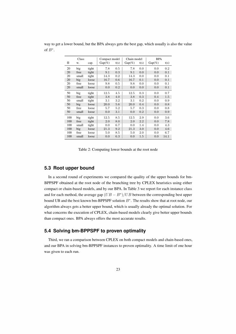
way to get a lower bound, but the BPA always gets the best gap, which usually is also the valueof B∗.

Class Compact model Chain model BPA|I| w. cap. Gap(%) t(s) Gap(%) t(s) Gap(%) t(s)

20 big tight 7.8 0.5 7.8 0.0 0.0 0.220 free tight 9.1 0.3 9.1 0.0 0.0 0.120 small tight 14.3 0.2 14.3 0.0 0.0 0.120 big loose 16.7 0.6 16.7 0.1 0.0 0.120 free loose 9.8 0.5 9.8 0.0 0.0 0.120 small loose 0.0 0.2 0.0 0.0 0.0 0.1



Table 2: Computing lower bounds at the root node

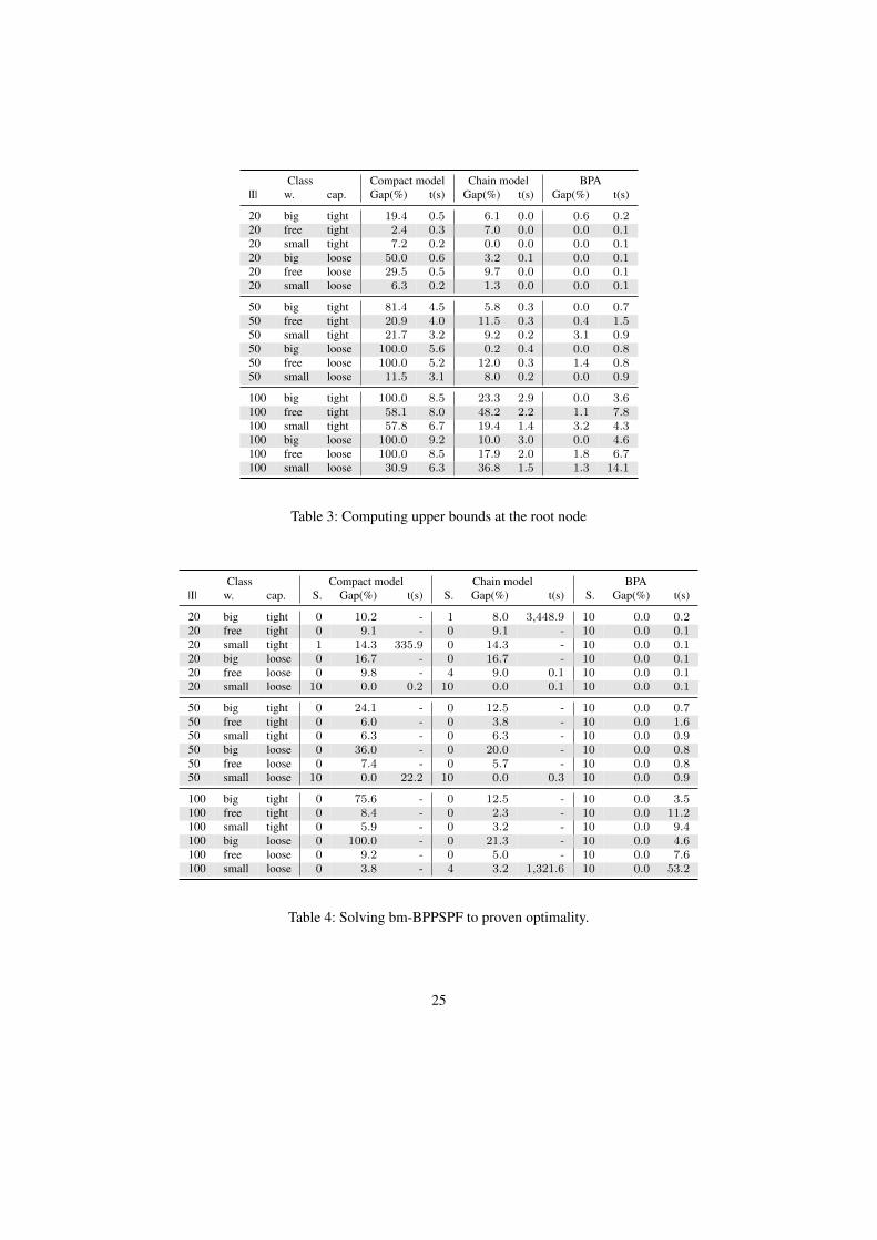
5.3 Root upper bound

In a second round of experiments we compared the quality of the upper bounds for bm-BPPSPF obtained at the root node of the branching tree by CPLEX heuristics using eithercompact or chain-based models, and by our BPA. In Table 3 we report for each instance classand for each method, the average gap (UB −B∗)/UB between the corresponding best upperbound UB and the best known bm-BPPSPF solution B∗. The results show that at root node, ouralgorithm always gets a better upper bound, which is usually already the optimal solution. Forwhat concerns the execution of CPLEX, chain-based models clearly give better upper boundsthan compact ones. BPA always offers the most accurate results.

5.4 Solving bm-BPPSPF to proven optimality

Third, we ran a comparison between CPLEX on both compact models and chain-based ones,and our BPA in solving bm-BPPSPF instances to proven optimality. A time limit of one hourwas given to each run.

23

In Table 4 we report for each solving method the number of instances solved to provenoptimality within the time limit (S), the average duality gap on the remaining ones computed as(UB − LB)/UB (Gap), and the average computing time (t).

Our BPA solves all the 180 instances, while CPLEX solves only 21 and 29 of them, usingthe compact and the chain-based models, respectively. This test confirms the results of [4] onthe hardness of BPPIF for generic solvers. Chain-based models perform better than compactones, always yielding a smaller duality gap.

5.5 Solving Size-Increasing variants

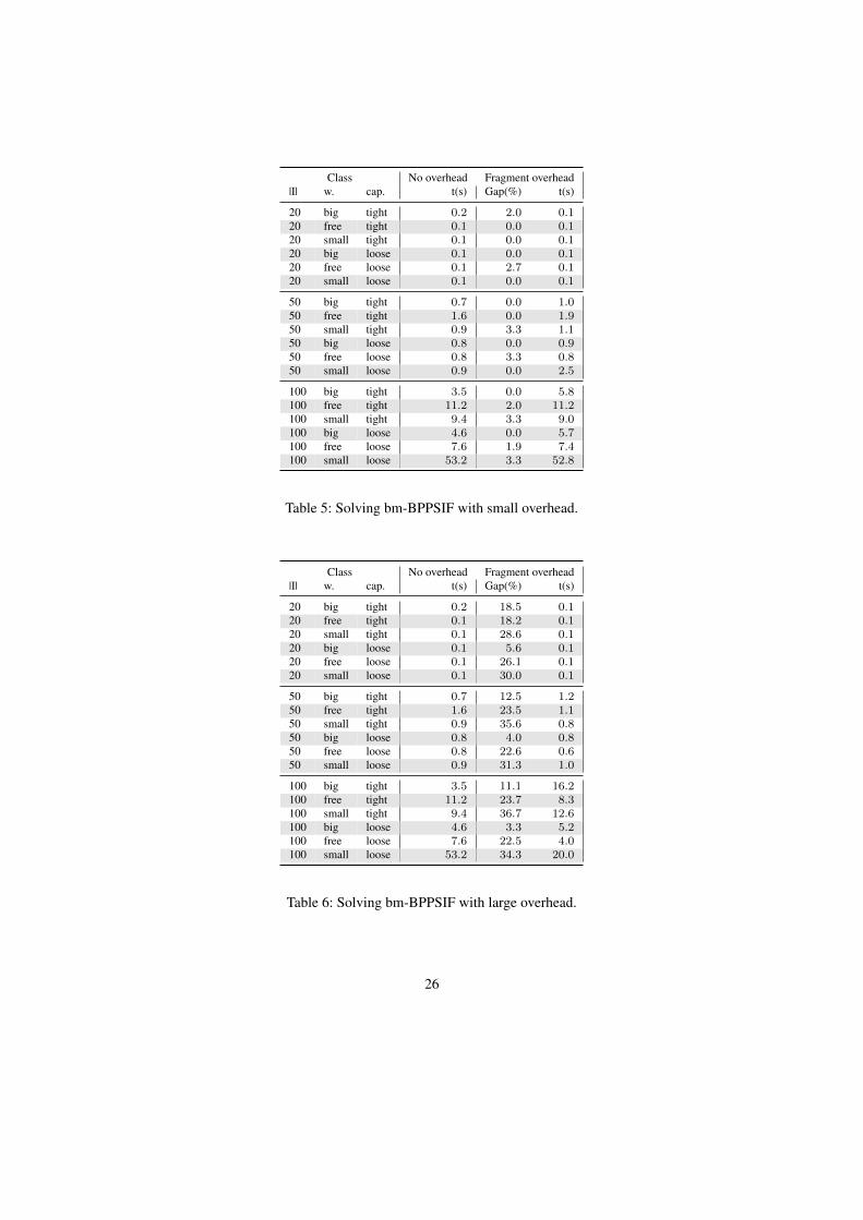
In the last round of experiments we assessed the impact of size-increasing features both onthe computational behavior of our algorithms and on the final solution costs. The analysis hasbeen performed using BPA. No time limit was given to these test, in order to always obtain aglobal optimal solution. Nevertheless, no test exceeded one hour of computation. The overheadε was set to be 1% of the bin capacity.

In Table 5 we report the average gap between the optimal solutions values obtained on thebm-BPPIF with the size preserving model (SP) and the ones obtained with the size-increasingvariant (SI), computed as (SI - SP)/SP.

From the results we observe that overhead mildly worsens the quality of the solutions, whilethe execution times are actually insensitive of the overhead management policy.

As a computational stress test, we repeated the experiment by increasing the overhead ε to10% of the bin capacity, although in practical applications such a large overhead would not bemeaningful. In Table 6 we report our results.

Still, no optimization required more than one hour of computing time. It is first interesting tonote that more aggressive overhead settings do not necessarily result in more difficult problemsfrom the computing time point of view. The solutions quality, instead, is highly penalized bythe large overhead: solutions are in a few cases more than 30% worse than their size-preservingcounterpart. We also observed that the impact of high overhead increases as the average itemsize decrease. In fact, for small items, an overhead of ε = 0.1 · C means an average growth ofone third of each item.

We finally performed the same test on the fm-BPPIF. When setting large overhead (ε =

0.1 · C), the fraction of infeasible instances was too large to provide any meaningful result,since for most instances the sum of the items weight plus the overhead of each item wasalready greater than the available capacity. Therefore, in Table 7 we report the results for smalloverhead (ε = 0.01 · C) only.

All instances having tight capacity resulted infeasible by design: it is however interesting to

24

Class Compact model Chain model BPA|I| w. cap. Gap(%) t(s) Gap(%) t(s) Gap(%) t(s)




Table 3: Computing upper bounds at the root node

Class Compact model Chain model BPA|I| w. cap. S. Gap(%) t(s) S. Gap(%) t(s) S. Gap(%) t(s)

20 big tight 0 10.2 - 1 8.0 3,448.9 10 0.0 0.220 free tight 0 9.1 - 0 9.1 - 10 0.0 0.120 small tight 1 14.3 335.9 0 14.3 - 10 0.0 0.120 big loose 0 16.7 - 0 16.7 - 10 0.0 0.120 free loose 0 9.8 - 4 9.0 0.1 10 0.0 0.120 small loose 10 0.0 0.2 10 0.0 0.1 10 0.0 0.1

50 big tight 0 24.1 - 0 12.5 - 10 0.0 0.750 free tight 0 6.0 - 0 3.8 - 10 0.0 1.650 small tight 0 6.3 - 0 6.3 - 10 0.0 0.950 big loose 0 36.0 - 0 20.0 - 10 0.0 0.850 free loose 0 7.4 - 0 5.7 - 10 0.0 0.850 small loose 10 0.0 22.2 10 0.0 0.3 10 0.0 0.9

100 big tight 0 75.6 - 0 12.5 - 10 0.0 3.5100 free tight 0 8.4 - 0 2.3 - 10 0.0 11.2100 small tight 0 5.9 - 0 3.2 - 10 0.0 9.4100 big loose 0 100.0 - 0 21.3 - 10 0.0 4.6100 free loose 0 9.2 - 0 5.0 - 10 0.0 7.6100 small loose 0 3.8 - 4 3.2 1,321.6 10 0.0 53.2

Table 4: Solving bm-BPPSPF to proven optimality.

25

Class No overhead Fragment overhead|I| w. cap. t(s) Gap(%) t(s)

20 big tight 0.2 2.0 0.120 free tight 0.1 0.0 0.120 small tight 0.1 0.0 0.120 big loose 0.1 0.0 0.120 free loose 0.1 2.7 0.120 small loose 0.1 0.0 0.1



Table 5: Solving bm-BPPSIF with small overhead.





Table 6: Solving bm-BPPSIF with large overhead.

26

note that infeasibility is detected quickly by our algorithms. In the remaining instances, thepenalties are in a few cases very high, confirming the behavior on bm-BPPSPF. The computingtime showed to be not an issue: all instances were solved within five minutes, even if byintroducing overhead the required CPU time slightly increased.


20 big tight 0.2 - 0.120 free tight 0.1 - 0.120 small tight 0.1 - 0.020 big loose 0.1 5.0 0.120 free loose 0.1 40.0 0.120 small loose 0.0 0.0 0.0



Table 7: Solving fm-BPPSIF with small overhead.

6 Conclusions

In this paper we tackled several variants of BPPIF with a unified approach: after collectingand deriving some properties of BPPIF solutions, we proposed new mathematical programmingmodels that avoid the use of fractional variables. Then, by using Dantzig-Wolfe decompositionwe also introduced an extended formulation and exploited column generation with ad-hocpricing algorithms, dual cuts, heuristics and implicit enumeration to design a new exact branch-and-price algorithm.

That algorithm proved to be first of all flexible, as minor or no modifications are needed toadapt it to bin-minimization or fragmentations-minimization, and to size preserving or sizeincreasing overhead management policies.

Our experimental campaign revealed that state-of-art general purpose solvers like CPLEXfind it beneficial to use our new models, but still fail in optimizing even instances of very small

27

size, regardless on the BPPIF variant considered. Instead, our algorithms proved to be veryeffective, being able to solve to proven optimality all the instances in our datasets in minutes ofcomputation for any BPPIF variant, thus outperforming both CPLEX and previous approachesfrom the literature.

Finally, having such an effective tool, we could perform an experimental comparison onoverhead handling, showing that overhead can be tackled explicitly without additional comput-ing effort, and with limited increase in solution costs, unless its amount becomes a substantialshare of the overall available capacity.

Of course, other BPPIF variants might be pertinent in practice, as the minimization of binsincluding fragmented items, the minimization of fragmented items, or more involved overheadmanagement schemes. We are currently investigating on how far our theoretical results andalgorithms might be extended.

References

[1] T. Achterberg. Scip: solving constraint integer programs. Mathematical Programming

Computation, 1(1):1 – 41, 2009.

[2] C. Archetti, N. Bianchessi, and M.G. Speranza. Branch-and-cut algorithms for the splitdelivery vehicle routing problem. European Journal of Operational Research, 238(3):685–698, 2014.

[3] M. Casazza and A. Ceselli. Improved algorithms for bin packing problems with itemfragmentation. In Contribution at EURO XXVI, Rome – July 2013, 2013.

[4] M. Casazza and A. Ceselli. Mathematical programming algorithms for bin packingproblems with item fragmentation. Computers & Operations Research, 46(0):1 – 11,2014.

[5] F. Chung, R. Graham, J. Mao, and G. Varghese. Parallelism versus memory allocationin pipelined router forwarding engines. Theory of Computer Systems, 39(6):829 – 849,2006.

[6] J.F. Cordeau, G. Laporte, M.W.P. Savelsbergh, and D. Vigo. Vehicle Routing, volume 14 ofHandbooks in Operations Research and Management Science, pages 367 – 428. Elsevier,2007.

[7] G.B. Dantzig and P. Wolfe. Decomposition principle for linear programs. Operations

research, 8:101–111, 1960.

28

[8] J.M.V. de Carvalho. Lp models for bin packing and cutting stock problems. European

Journal of Operational Research, 141(2):253 – 273, 2002.

[9] M. Dell’Amico, J. C. Díaz Díaz, and M. Iori. The bin packing problem with precedenceconstraints. Operations Research, 60:1491–1504, 2012.

[10] CPLEX development team. Ibm ilog cplex optimization studio: Cplex user’s manual -version 12 release 4. Technical report, IBM corp., 2011.

[11] L. Epstein, A. Levin, and R. van Stee. Approximation schemes for packing splittableitems with cardinality constraints. Algorithmica, 62(1 – 2):102 – 129, 2012.

[12] L. Epstein and R. van Stee. Improved results for a memory allocation problem. Theory of

Computing Systems, 48(1):79 – 92, 2011.

[13] P. C. Gilmore and R. E. Gomory. A linear programming approach to the cutting-stockproblem. Operations Research, 9:849–859, 1961.

[14] T. Gschwind and S. Irnich. Dual inequalities for stabilized column generation revis-ited. Technical Report Working Paper n. 1407, Gutenberg School of Management andEconomics, Mainz Univ., 2014.

[15] S. C. Ho and W. Y. Szeto. Solving a static repositioning problem in bike-sharing systemsusing iterated tabu search. Transportation Research Part E: Logistics and Transportation

Review, 69:180–198, 2014.

[16] C.A. Mandal, P.P. Chakrabarti, and S. Ghose. Complexity of fragmentable object binpacking and an application. Computers and Mathematics with Applications, 35(11):91––97, 1998.

[17] S. Martello and P. Toth. Knapsack problems: algorithms and computer implementations.John Wiley & Sons, Inc., New York, NY, USA, 1990.

[18] M. A. Alba Martínez, F. Clautiaux, M. Dell’Amico, and M. Iori. Exact algorithms for thebin packing problem with fragile objects. Discrete Optimization, 10(3):210–223, 2013.

[19] N. Menakerman and R. Rom. Bin packing with item fragmentation. In Proceedings of

the 7th International Workshop on Algorithms and Data Structures, in: Lecture Notes in

Computer Science, pages 313–324, 2001.

[20] M. Schneider, A. Stenger, and D. Goeke. The electric vehicle-routing problem with timewindows and recharging stations. Transportation Science, 48(4):500–520, 2014.

29

[21] S. Secci, A. Ceselli, F. Malucelli, A. Pattavina, and B. Sansò. Direct optimal design of aquasi-regular composite-star core network. In IEEE Proc. of DRCN, pages 7–10, 2007.

[22] H. Shachnai, T. Tamir, and O. Yehezkely. Approximation schemes for packing with itemfragmentation. In Thomas Erlebach and Giuseppe Persinao, editors, Approximation and

Online Algorithms, volume 3879 of Lecture Notes in Computer Science, pages 334–347.Springer Berlin / Heidelberg, 2006.

[23] N. Skorin-Kapov. Routing and wavelength assignment in optical networks using binpacking based algorithms. European Journal of Operational Research, 177(2):1167–1179,2007.

[24] José M. Valério de Carvalho. Using extra dual cuts to accelerate column generation.INFORMS Journal on Computing, 17(2):175–182, 2005.

30

exactly solving packing problems with fragmentation

Documents