Exact Spectral - Like Gradient Method forDistributed Optimization

Dusan Jakovetic ∗ Natasa Krejic ∗

Natasa Krklec Jerinkic ∗

August 18, 2019Abstract

Since the initial proposal in the late 80s, spectral gradient methodscontinue to receive significant attention, especially due to their excel-lent numerical performance on various large scale applications. How-ever, to date, they have not been sufficiently explored in the contextof distributed optimization. In this paper, we consider unconstraineddistributed optimization problems where n nodes constitute an arbi-trary connected network and collaboratively minimize the sum of theirlocal convex cost functions. In this setting, building from existing ex-act distributed gradient methods, we propose a novel exact distributedgradient method wherein nodes’ step-sizes are designed according tothe novel rules akin to those in spectral gradient methods. We re-fer to the proposed method as Distributed Spectral Gradient method(DSG). The method exhibits R-linear convergence under standard as-sumptions for the nodes’ local costs and safeguarding on the algorithmstep-sizes. We illustrate the method’s performance through simulationexamples.

Keywords: Distributed optimization, spectral gradient, R-linear con-vergence.

AMS subject classification. 90C25, 90C53, 65K05

∗Department of Mathematics and Informatics, Faculty of Sciences, University of NoviSad, Trg Dositeja Obradovica 4, 21000 Novi Sad, Serbia. e-mail: {djakovet@uns.ac.rs,natasak@uns.ac.rs, natasa.krklec@dmi.uns.ac.rs}. Research supported by the SerbianMinistry of Education, Science, and Technological Development, Grant no. 174030. Thework was also supported in part by the European Union (EU) Horizon 2020 project I-BiDaaS, project number 780787.

1

1 Introduction

We consider a connected network with n nodes, each of which has access toa local cost function fi : Rd → R, i = 1, . . . , n. The objective for all nodes isto minimize the aggregate cost function f : Rd → R, defined by

f(y) =n∑i=1

fi(y). (1)

Problems of this form attract a lot of scientific interest as they arisein many emerging applications like distributed inference in sensor networks[29, 16, 18, 8], distributed control, [22], distributed learning, e.g., [7], etc.

For example, with distributed supervised learning, a training data set ispartitioned into n blocks which correspond to distinct nodes in the network(e.g., servers, nodes in a computer cluster, etc.) The goal is then to train amachine learning model based on the data by all nodes without transferringdata to a single location, due to, e.g., storage limitations or privacy concerns.In this context, function fi(·) is the empirical loss with respect to the dataavailable at node i:

fi(x) =∑j∈Ji

`i (x, Di,j) +Ri(x),

where Di,j is a data sample at node i, j ∈ Ji, Ji is the indices set ofnode i’s data samples, `i(·, ·) is the loss function at node i (e.g., logistic,quadratic, hinge, etc.), and Ri(·) is the regularization function at node i(e.g., the quadratic regularization). More concretely, with L2-regularizedlogistic losses, we have:

`i (x, Di,j) = ln(1 + exp(−bi(a>i x))

), Ri(x) =

c

2‖x‖2.

Here, ‖ · ‖ stands for the 2-norm, Di,j = (ai,j, bi,j), where ai,j ∈ Rd is afeature vector, bi,j ∈ {−1,+1} is the corresponding class label, and c > 0 isthe regularization tuning parameter; see, e.g., [7].

To solve this and related problems several distributed first order methods,e.g., [25, 8, 13], and second order methods, e.g., [19, 20, 15], have beenproposed. The methods of this type converge to an approximate solutionof problem (1) if a constant (non-diminishing) step size is used; they can beinterpreted through a penalty-like reformulation of (1); see [14, 19] for details.

2

Convergence to an exact solution can be achieved by using diminishing step-sizes, but this comes at a price of slower convergence.

More recently, exact distributed first order methods, e.g., [31, 12, 30, 26,11], and second order methods, e.g., [21, 20], have been proposed, that con-verge to the exact solution under constant step sizes. The method in [30] usestwo different weight matrices, differently from the standard distributed gra-dient method that utilizes a single weight matrix. The methods in [26, 23, 24]implement tracking of the network-wide average gradient and correct the dy-namics of the standard distributed method [25] by replacing the nodes’ localgradients with the tracked global average gradient estimates. A unification ofa class of exact first order methods and some further improvements are pre-sented in [11]. References [31, 23] study exact methods with uncoordinatedstep-sizes, while reference [12] proposes exact methods for non-convex prob-lems. An exact distributed second order method has been developed in [21].We refer to [11] for a detailed review of other works on exact distributedmethods.

Spectral gradient methods are a popular class of methods in centralized op-timization due to their simplicity and efficiency. The class originated with theproposal of the Barzilei-Borwein method [1] and its analysis therein for two-dimensional convex quadratic functions, while the method has been subse-quently extended to more general optimization problems, both unconstrainedand constrained, [27, 28, 6]. Spectral gradient methods can be viewed as amean to incorporate second-order information in a computationally efficientmanner into gradient descent methods. In practice, they achieve significantlyfaster convergence with respect to standard gradient methods while the addi-tional computational overhead per iteration is very small. Roughly speaking,the main idea of spectral gradient methods is to approximate the Hessian ateach iteration with a scalar matrix (the leading scalar of the matrix is calledthe spectral coefficient) that approximately fits the secant equation. Calcu-lating the spectral gradient’s scalar matrix is much cheaper than evaluationof the Newton direction while the convergence speed is usually much betterthan that of the gradient method. Spectral methods are characterized bya non-monotone behaviour which makes them suitable for combination withnon-monotone line search methods, [28]. It was demonstrated in [28] that thespectral gradient method can be more efficient than the conjugate gradientmethod for certain classes of optimization problems. The R-linear conver-gence rate was established in [9], while extensions to constrained optimizationin the form of Spectral Projected Gradient (SPG) methods are developed in

3

[3, 4, 5]. A vast number of applications is available in the literature, and acomprehensive overview is presented in [6].

The principal aim of this paper is to provide a generalization of spectralgradient methods to distributed optimization and give preliminary numericaltests of its efficiency. Extension of spectral gradient methods to a distributedsetting is a highly nontrivial task. We develop an exact method (converg-ing to the exact solution) that we refer to as Distributed Spectral Gradientmethod (DSG). The method utilizes step-sizes that are akin to those of cen-tralized spectral methods. The spectral-like step-sizes are embedded into theexact distributed first order method in [26]; see also [23, 24]. We utilize theprimal-dual interpretation of the method in [26] – as provided in [11] (seealso [24]) – and the corresponding form of the error recursion equation. Ananalogy with the error recursion of the conventional spectral method statedin [27] is exploited to define the time-varying, node dependent, algorithmstep-sizes. This analogy also allows for an intuitive interpretation of theproposed method.

We show that the proposed DSG method exhibits R-linear convergencerate under appropriate assumptions on the nodes’ local objectives, static,undirected networks, and appropriate safeguarding of the step-sizes.

The proposed DSG method has several favorable features. Namely, sim-ulations suggest that DSG converges under a significantly wider range ofadmissible step-sizes than existing exact first order methods like [26, 23]. In-deed, existing methods require for convergence that step-sizes be sufficientlysmall, both in theory and in practical implementations. We show by simu-lation examples that DS converges for step-size ranges which are orders ofmagnitude broader than the admissible step-size ranges of [23]. We furthershow analytically on a consensus problem-special case, under a special struc-ture of the underlying weight matrix W , that DSG converges without any apriory upper bound on the step-sizes and with a lower bound on the step-sizes, while the method in [26] diverges on the same example for the step-sizelarger than two.

Another important feature of the DSG method is that it adaptivelyadjusts the step-sizes over iterations such that good convergence speed isachieved. This eliminates the need to hand-optimize and/or align before-hand the step-size values across nodes, as it is the case with existing meth-ods like [26]. This beforehand tuning may be expensive, resource-consuming,and tedious process, in many scenarios. In contrast, the proposed methodrequires only a coarse estimate (to within a factor of 10-100, for example) of

4

the nodes’ gradients’ Lipschitz constant beforehand. We compare the per-formance of DSG by simulation with [26] under a hand-optimized step-size.While the latter method with hand-optimized step-size may converge fasterthan DSG, it may also converge worse than DSG, when the step-size of [26]is chosen poorly. Therefore, when aligning and hand-tuning of step-sizes isnot feasible beforehand, the proposed method represents a valuable choice.

The paper is organized as follows. Some preliminary considerations andassumptions are presented in Section 2. The proposed distributed spectralmethod (DSG) is introduced in Section 3, while the convergence theory isdeveloped in Section 4. Initial numerical tests are presented in Section 5, andsome conclusions are drawn in Section 6. Some auxiliary proofs are relegatedto the Appendix.

2 Model and preliminaries

The network and optimization models that we assume are described in Sub-section 2.1. The proposed method is based on the distributed gradientmethod developed in [26] and the centralized spectral gradient method [27]which are briefly reviewed in Subsection 2.2 and 2.3. The convergence anal-ysis is based on the Small Gain Theorem which is stated in Subsection 2.4.

2.1 Optimization and network models

We impose a set of standard assumptions on the functions fi in (1) and onthe underlying network.Assumption A1. Assume that each local function fi : Rd → R, i = 1, . . . , nis twice continuously differentiable and for all i = 1, . . . , n and all y ∈ Rp,there holds

µiI � ∇2fi(y) � liI (2)

where li ≥ µi ≥ 0 and µ :=∑n

i=1 µi > 0.Here, notation Γ � Υ means that matrix (Υ−Γ) is positive semi-definite.

This implies that the gradients of the fi’s are Lipschitz continuous with con-stants li and that the full gradient ∇f is Lipschitz continuous with constant

L :=n∑i=1

li. (3)

5

Moreover, under the Assumption A1, the objective function f is µ-stronglyconvex and problem (1) is solvable and has a unique solution, denoted by y∗.For future reference, let us introduce the function F : Rnd → R, defined by:

F (x) =n∑i=1

fi(xi), (4)

where x ∈ Rnd consists of n blocks xi ∈ Rd, i.e., x = ((x1)T , ..., (xn)T )T .Assumption A1 clearly implies that ∇F is Lipschitz continuous, where aLipschitz constant can be taken as maxi=1,...,n li. For the sake of simplicity,we retain the same Lipschitz constant as for ∇f , i.e., for any y, z ∈ Rnd,there holds:

‖∇F (y)−∇F (z)‖ ≤ L‖y − z‖, (5)

where L is defined by (3).We assume that the network of nodes is an undirected network G = (V , E),

where V is the set of nodes and E is the set of edges, i.e., all pairs {i, j}of nodes which can exchange information through a communication link.Assumption A2. The network G = (V , E) is connected, undirected andsimple (no self-loops nor multiple links).

Let us denote by Oi the set of nodes that are connected with node ithrough a direct link (neighborhood set), and let Oi = Oi

⋃{i}. Associate

with G a symmetric, doubly stochastic n × n matrix W. The elements ofW are all nonnegative and both rows and columns sum up to one. Moreprecisely, the following is assumed.Assumption A3. The matrix W = W T ∈ Rn×n is doubly stochastic, withelements wij such that

wij > 0 if {i, j} ∈ E , wij = 0 if {i, j} /∈ E , i 6= j, and wii = 1−∑j∈Oi

wij

and there exist constants wmin and wmax such that for i = 1, . . . , n

0 < wmin ≤ wii ≤ wmax < 1.

Denote by λ1 ≥ . . . ≥ λn the eigenvalues of W. It can be shown thatλ1 = 1, and |λi| < 1, i = 2, ..., n.

For future reference, define the n × n matrix J that has all the entriesequal 1/n. We refer to J as the ideal consensus matrix; see, e.g., [17]. Also,

6

introduce the (nd)×(nd) matrixW = W⊗I, where ⊗ denotes the Kroneckerproduct and I is the identity matrix from Rd×d. It can be seen that d×d blockon the (i, j)-th position of the matrixW equals to wij I. By properties of theKronecker product, the eigenvalues of W are λ1, ..., λn, each one occurringwith the multiplicity d. We also introduce the (nd)× (nd) matrix J = J⊗I,where, as before, J is the n × n ideal consensus matrix, and I is the d × didentity matrix. Also, we denote by I the (nd)× (nd) identity matrix.

2.2 Exact Distributed first order method

Let us now briefly review the distributed first order method in [26]; seealso [23, 24]. These methods serve as a basis for the development of theproposed distributed spectral gradient method. The method in [26] maintainsover iterations k = 0, 1, ..., at each node i, the solution estimate xki ∈ Rd andan auxiliary variable zki ∈ Rd. Specifically, the update rule is as follows

xk+1i =

∑j∈Oi

wij x(k)j − α zki (6)

zk+1i =

∑j∈Oi

wij z(k)j +

(∇fi(xk+1

i )−∇fi(xki )), k = 0, 1, ... (7)

Here, α > 0 is a constant step-size; the initialization x0i , i = 1, ..., n, is

arbitrary, while z0i = ∇fi(x0

i ), i = 1, ..., n. Equation (6) shows that eachnode i, as with standard distributed gradient method [25], makes two-foldprogress: 1) by weight-averaging its solution estimate with its’ neighbors;and 2) by taking a step opposite to the estimated gradient direction. Thestandard distributed gradient method in [25] takes a negative step in thedirection of ∇fi(xki ), while the method in [26] makes a step in direction ofzki . This vector serves as a tracker of the network-wide gradient

∑ni=1∇fi(xki ).

This modification in the update rule enables convergence to the exact solutionunder a constant step-size [26].

It is useful to represent method (6)–(7) in vector format. Let xk ∈ Rnd,zk ∈ Rnd, and recall function F in (4) and matrix W = W ⊗ I. Then, themethod (6)–(7) in the vector form becomes

xk+1 = W x(k) − α zk (8)

zk+1 = W z(k) +(∇F (xk+1)−∇F (xk)

), k = 0, 1, ..., (9)

with arbitrary x0 and z0 = ∇F (x0).

7

The method (8)–(9) allows for a primal-dual interpretation; see [11] andalso [24] for a similar interpretation. The primal-dual interpretation will beimportant for the development of the proposed distributed spectral gradientmethod. Namely, it is demonstrated in [11] that (8)–(9) is equivalent to thefollowing update rule

xk+1 = Wxk − α(∇F (xk) + uk) (10)

uk+1 = Wuk + (W − I)∇F (xk), (11)

with variable u0 = 0 ∈ Rdn and arbitrary x0. It can be shown that, under ap-propriately chosen step-size α, the sequence {xk} converges to x∗ := 1⊗y∗ =( (y∗)T , ..., (y∗)T )T , and uk converges to−∇F (1⊗y∗) = −(∇f1(y∗)T , ...,∇fn(y∗)T )T .Here, 1 ∈ Rn is the vector with all components equal to one.

2.3 Centralized spectral gradient method

Let us briefly review the spectral gradient (SG) method in centralized opti-mization. Consider the unconstrained minimization problem with a genericobjective function φ : Rd → R which is continuously differentiable. Let theinitial solution estimate be arbitrary x0 ∈ Rd. The SG method generates thesequence of iterates {xk} as follows

xk+1 = xk − σ−1k ∇φ(xk), k = 0, 1, . . . , (12)

where the initial spectral coefficient σ0 > 0 is arbitrary and σk, k = 1, 2, ...,is given by

σk = P[σmin,σmax ](σ′k), σ′k =

(sk−1)Tyk−1

(sk−1)T sk−1. (13)

Here, 0 < σmin < σmax < +∞ are given constants, sk−1 = xk − xk−1, yk−1 =∇φ(xk)−∇φ(xk−1), and P[a,b] stands for the projection of a scalar onto theinterval [a, b]. The projection onto the interval [σmin, σmax] is the safeguardingthat is necessary for convergence. The spectral coefficient σ′k is derived asfollows. Assume that the Hessian approximation in the form Bk = σkI. Thenthe approximate secant equation

Bksk−1 ≈ yk−1 (14)

can be solved in the least square sense. It is easy to show that least squaressolution of (14) yields exactly (13). For future reference, we briefly review the

8

result on the evolution of error for the SG method stated in [27]. Considerthe special case of a strongly convex quadratic function φ(x) = 1

2xTAx+ bTx

for a symmetric positive definite matrix A, and denote by ek := x∗ − xk theerror at iteration k, where x? is the minimizer of φ. Then, it can be shownthat the error evolution can be expressed as [27]:

ek+1 = (I − σ−1k A)ek. (15)

The above relation will play a key role in the intuitive explanation of thedistributed spectral gradient method proposed in this paper.

2.4 Small gain theorem

Convergence analysis of the proposed method will be based upon the SmallGain Theorem, e.g. [10]. This technique has been previously used and provedsuccessful for the analysis of exact distributed gradient methods in, e.g., [23,24]. We briefly introduce the concept here, while more details are availablein [10, 23].

Denote by a := a1, a2, . . . an infinite sequence of vectors, ak ∈ Rd, k =0, 1, . . . . For a fixed δ ∈ (0, 1), define

‖a‖δ,K = maxk=0,1,...,K

{ 1

δk‖ak‖}

‖a‖δ = supk≥0{ 1

δk‖ak‖}.

Obviously, for any K ′ ≥ K ≥ 0 we have ‖a‖δ,K ≤ ‖a‖δ,K′ ≤ ‖a‖δ. Also,if ‖a‖δ is finite for some δ ∈ (0, 1) than the sequence a converges to zeroR-linearly. We present the Small Gain Theorem in a simplified form thatinvolves only two sequences, as this will suffice for our considerations; formore general forms of the result see [10, 23].

Theorem 2.1. [10, 23]. Consider two infinite sequences a = a0, a1, . . . , b =b0, b1, . . . , with ak, bk ∈ Rd, k = 0, 1, . . . . Suppose that for some δ ∈ (0, 1)and for all K = 0, 1, . . . , there holds

‖a‖δ,K ≤ γ1‖b‖δ,K + w1

‖b‖δ,K ≤ γ2‖a‖δ,K + w2,

9

where γ1 · γ2 ∈ [0, 1). Then

‖a‖δ ≤ 1

1− γ1γ2

(w1γ2 + w2).

Furthermore, limk→∞ ak = 0 R-linearly.

Following, for example, the proof of Lemma 6 in [11] (see also [23]), it iseasy to derive the result below.

Lemma 2.1. Consider three infinite sequence a = a0, a1, . . . , b = b0, b1, . . . , c =c0, c1, . . . with ak, bk, ck ∈ Rd, k = 0, 1, . . . . Suppose that there holds

‖ak+1‖ ≤ c1‖ak‖+ c2‖bk‖+ c3‖ck‖, k = 0, 1, . . .

where c1, c2, c3 ≥ 0. Then, for all K = 0, 1, . . . and 0 ≤ c1 < δ < 1,

‖a‖δ,K ≤ c2

δ − c1

‖b‖δ,K +c3

δ − c1

‖c‖δ,K +δ

δ − c1

‖a0‖.

3 Spectral gradient method for distributed

optimization

3.1 The algorithm

Let us now present the proposed Distributed Spectral Gradient, DSG, method.The method incorporates spectral-like step size policy into (8)–(9). The step-sizes are locally computed and vary both across nodes and across iterations.As (8)–(9), the DSG method maintains the sequence of solution estimatesxk ∈ Rnd and an auxiliary sequence zk ∈ Rnd. Specifically, the update ruleis as follows

xk+1 = W xk − Σ−1k zk (16)

zk+1 = W zk +(∇F (xk+1)−∇F (xk)

), k = 0, 1, ... (17)

The initial solution estimate x0 is arbitrary, while z0 = ∇F (x0). Here,

Σk = diag(σk1 I, . . . , σ

kn I),

10

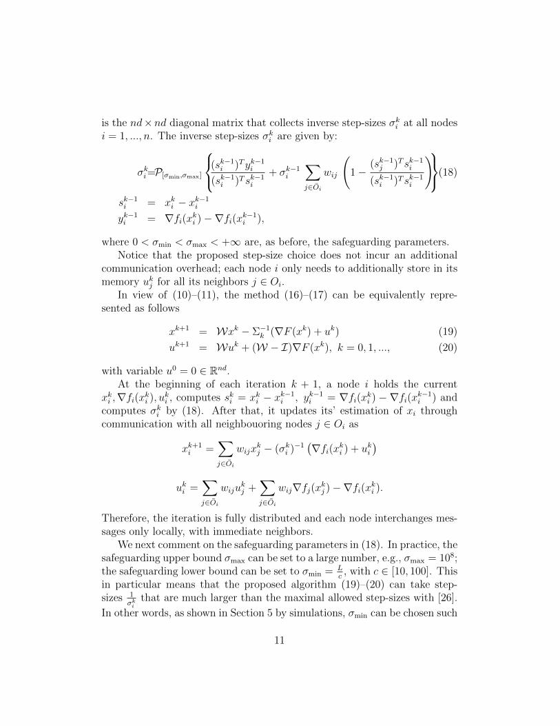
is the nd×nd diagonal matrix that collects inverse step-sizes σki at all nodesi = 1, ..., n. The inverse step-sizes σki are given by:

σki=P[σmin,σmax]

(sk−1i )Tyk−1

i

(sk−1i )T sk−1

i

+ σk−1i

∑j∈Oi

wij

(1−

(sk−1j )T sk−1

i

(sk−1i )T sk−1

i

)(18)

sk−1i = xki − xk−1

i

yk−1i = ∇fi(xki )−∇fi(xk−1

i ),

where 0 < σmin < σmax < +∞ are, as before, the safeguarding parameters.Notice that the proposed step-size choice does not incur an additional

communication overhead; each node i only needs to additionally store in itsmemory ukj for all its neighbors j ∈ Oi.

In view of (10)–(11), the method (16)–(17) can be equivalently repre-sented as follows

xk+1 = Wxk − Σ−1k (∇F (xk) + uk) (19)

uk+1 = Wuk + (W − I)∇F (xk), k = 0, 1, ..., (20)

with variable u0 = 0 ∈ Rnd.At the beginning of each iteration k + 1, a node i holds the current

xki ,∇fi(xki ), uki , computes ski = xki − xk−1i , yk−1

i = ∇fi(xki ) − ∇fi(xk−1i ) and

computes σki by (18). After that, it updates its’ estimation of xi throughcommunication with all neighbouoring nodes j ∈ Oi as

xk+1i =

∑j∈Oi

wijxkj − (σki )−1

(∇fi(xki ) + uki

)uki =

∑j∈Oi

wijukj +

∑j∈Oi

wij∇fj(xkj )−∇fi(xki ).

Therefore, the iteration is fully distributed and each node interchanges mes-sages only locally, with immediate neighbors.

We next comment on the safeguarding parameters in (18). In practice, thesafeguarding upper bound σmax can be set to a large number, e.g., σmax = 108;the safeguarding lower bound can be set to σmin = L

c, with c ∈ [10, 100]. This

in particular means that the proposed algorithm (19)–(20) can take step-sizes 1

σki

that are much larger than the maximal allowed step-sizes with [26].

In other words, as shown in Section 5 by simulations, σmin can be chosen such

11

that the method in [26] with step-size α = 1/σmin diverges, while the novelmethod (19)–(20) with time-varying step sizes and the safeguard lower boundσmin (hence potentially taking step-size values close or equal to 1/σmin) stillconverges.

3.2 Step-size derivation

We now provide a derivation and a justification of the step-size choice (18).For notational simplicity, assume for the rest of this Subsection that d = 1and thus W = W and J = J . Let each fi be a strongly convex quadraticfunction, i.e.,

fi(xi) =1

2hi(xi − bi)2,

and H = diag(h1, . . . , hn), hi > 0, for all i. Then, for the primal errorek := xk − x∗ and the dual error uk := uk +∇F (x∗), one can show that thefollowing recursion holds:[

ek+1

uk+1

]=

[W − Σ−1

k H −Σ−1k

(W − I)H W − J

]·[ek

uk

](21)

We now make a parallel identification between the error dynamics of the cen-tralized SG method for a strongly convex quadratic cost with leading matrixA given in (15) and the error dynamics of the proposed distributed methodin (21). Consider first the centralized SG method. The error dynamics matrixis given by I−σ−1

k A, while the (new) spectral coefficient is sought to fit the se-cant equation with least mean square deviation: σk(x

k−xk−1) = A(xk−xk−1).That is, the error dynamics matrix I − σ−1

k A is made small by letting σk Ibe a scalar matrix approximation for matrix A, i.e., solving

minσ>0‖σsk − yk‖2 = min

σ>0‖σsk − Ask‖2.

Now, consider the error dynamics of the proposed distributed method in (21),and specifically focus on the update for the primal error:

ek+1 =(W − Σ−1

k H)ek + Σ−1

k uk

=(I − Σ−1

k [Σk (I −W ) +H])ek + Σ−1

k uk. (22)

Notice that the second error equation in (21) does not depend on Σk. Com-paring (15) with (22), we first see that both the primal and the dual error

12

play a role in (22). The effect of the dual error uk can be controlled by mak-ing Σ−1

k small enough. This motivates the safeguarding of Σk from belowby σmin. Regarding the effect of the primal error ek, one can see that it influ-ences the error through the matrix I − Σ−1

k [Σk (I −W ) +H]. Analogouslyto the centralized SG case, this matrix can be made small by the followingidentification

A ≡ Σk (I −W ) +H, and σk ≡ Σk.

Therefore, we seek Σk+1 as the least mean squares error fit to the followingequation

Σk+1

(xk+1 − xk

)= (Σk(I −W ) +H)

(xk+1 − xk

). (23)

For generic (non-quadratic) cost functions, this translates into the following:

Σk+1

(xk+1 − xk

)= ( Σk(I −W ) )

(xk+1 − xk

)+(∇F (xk+1)−∇F (xk)

).

(24)The rationale behind the generalization from (23) to (24) is as follows.For quadratic functions, the term

(∇F (xk+1)−∇F (xk)

)equals precisely

H(xk+1 − xk

). Therefore, for quadratic functions, equations (23) and (24)

are identical. This motivates the argument that (24) can be viewed as a gen-eralization of (23). It is worth noting that a similar argument is used in [27]for motivating the spectral step-size choice for centralized gradient methods.

The (intermediate) inverse step-size matrix Σ′k+1 is now obtained by min-imizing∥∥Σk+1

(xk+1 − xk

)− ( Σk(I −W ) )

(xk+1 − xk

)−(∇F (xk+1)−∇F (xk)

)∥∥2.

(25)This leads to the step-size choice in (18). Finally, to ensure strictly positivestep-sizes on the one hand, and a bounded effect of the dual error on theother hand, Σ′k+1 is projected entry-wise onto the interval [σmin, σmax ].

4 Convergence analysis

In Subsection 4.1, we prove that the proposed DSG method, (19)-(20), con-verges to the solution of problem (1) provided that the spectral coefficients σkiare uniformly bounded with properly chosen constants. In Subsection 4.2,we then prove that the method converges without any a priori upper boundon the step-sizes and with a lower bound on the step-sizes, for a special caseof the assumed setting.

13

4.1 Analysis for the generic case in the presence ofsafeguarding

For the sake of simplicity, we will restrict our attention to one dimensionalcase, i.e., d = 1, while the general case is proved analogously. Hence, we haveW = W and J = J in this Section. The following notation and relationsare used. Recall that x∗ = 1 ⊗ y∗ where y∗ is the solution of (1). Definexk = xk − Jxk and xk = 1Txk/n. Then

xk = xk − 1

n11Txk = xk − 1⊗ xk.

Also, for ek = xk − x∗,

(I − J)ek = (I − J)xk − (I − J)x∗ = xk − x∗ + 1⊗ y∗ = xk.

Moreover, notice that J2 = J and therefore J(I − J) = 0, which furtherimplies Jxk = 0. Now, for W = W − J we obtain

W xk = (W − J)(I − J)xk = Wxk − Jxk = Wxk

and(I − J)Wek = W (I − J)ek = Wxk = W xk. (26)

Define ek = xk − y∗. So, the following equalities hold

ek = xk − 1⊗ xk + 1⊗ xk − 1⊗ y∗ = xk + 1⊗ ek. (27)

Given that W is doubly stochastic, there follows Wx∗ = x∗, 1TW = 1T

and 1T (W − I) = 0. So, multiplying (20) from the left with 1T , we obtainuk+1 = uk, where uk = 1Tuk/n. Since uk = 0, we conclude that

uk = 0, k = 0, 1, ... (28)

See Lemma 8 in [11] that applies here as well, since the update (20) is aspecial case of update (16) in [11], with B = 0 defined therein. Moreover,define uk = ∇F (x∗) + uk. Using the fact that 1T∇F (x∗) = 0 we obtain

Juk =1

n1⊗ (1Tuk + 1T∇F (x∗)) = Juk = 1⊗ uk = 0 (29)

Now, Assumption A1 together with the Mean value theorem implies that forall i = 1, 2, ..., n and k = 1, 2, ..., there exists θki such that

∇fi(xki )−∇fi(y∗) = ∇2fi(θki )(x

ki − y∗).

14

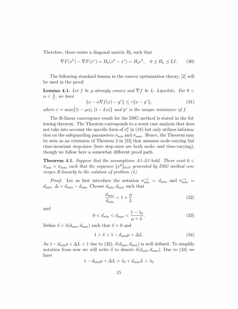
Therefore, there exists a diagonal matrix Hk such that

∇F (xk)−∇F (x∗) = Hk(xk − x∗) = Hke

k, 0 � Hk � LI. (30)

The following standard lemma in the convex optimization theory, [2] willbe used in the proof.

Lemma 4.1. Let f be µ-strongly convex and ∇f be L- Lipschitz. For 0 <α < 2

L, we have

‖x− α∇f(x)− y∗‖ ≤ τ‖x− y∗‖, (31)

where τ = max{|1− µα|, |1− Lα|} and y∗ is the unique minimizer of f .

The R-linear convergence result for the DSG method is stated in the fol-lowing theorem. The Theorem corresponds to a worst case analysis that doesnot take into account the specific form of σki in (18) but only utilizes informa-tion on the safeguarding parameters σmin and σmax. Hence, the Theorem maybe seen as an extension of Theorem 2 in [23] that assumes node-varying buttime-invariant step-sizes (here step-sizes are both node- and time-varying),though we follow here a somewhat different proof path.

Theorem 4.1. Suppose that the assumptions A1-A3 hold. There exist 0 <σmin < σmax such that the sequence {xk}k∈N generated by DSG method con-verges R-linearly to the solution of problem (1).

Proof. Let us first introduce the notation σ−1min = dmax and σ−1

max =dmin, ∆ = dmax − dmin. Choose dmin, dmax such that

dmax

dmin

< 1 +µ

L(32)

and

0 < dmin < dmax <1− λ2

µ+ L. (33)

Define δ = δ(dmin, dmax) such that δ > 0 and

1 > δ > 1− dminµ+ ∆L. (34)

As 1− dminµ+ ∆L < 1 due to (32), δ(dmin, dmax) is well defined. To simplifynotation from now we will write δ to denote δ(dmin, dmax). Due to (33) wehave

1− dminµ+ ∆L > λ2 + dmaxL > λ2

15

and hence

0 < δ − (1− dminµ+ ∆L) < δ − (λ2 + dmaxL) < δ − λ2. (35)

Notice further that δ− (1− dminµ+ ∆L) is a decreasing function of dmax and∆ and therefore decreasing dmax,∆ if needed does not violate 35 if (32-33) aresatisfied. In fact one can take dmax,∆ arbitrary small with the correspondingdmin without violating (32)-(35).

Denote Dk = Σ−1k and dki = (σki )−1 and notice that dki ≥ dmin. Subtracting

x∗ from both sides of (19) and using the fact that Wx∗ = x∗ we obtain

ek+1 = Wek−Dk(∇F (xk)+uk±∇F (x∗)) = Wek−Dk(∇F (xk)−∇F (x∗))−Dkuk.

From (30) we obtain

ek+1 = (W −DkHk)ek −Dku

k. (36)

Now, adding ∇F (x∗) on both sides of (20) we obtain

uk+1 = Wuk + (W − I)∇F (xk) +∇F (x∗)±W∇F (x∗)

= Wuk + (W − I)(∇F (xk)−∇F (x∗)). (37)

Using (29) and (30) we get

uk+1 = (W − J)uk + (W − I)Hkek. (38)

Taking the norm and using (27), we obtain

‖uk+1‖ ≤ λ2‖uk‖+ (1− λn)L(‖xk‖+√n|ek|). (39)

Lemma 2.1 with c1 = λ2, c2 = c3 = (1− λn)L yields

‖u‖δ,K ≤ c2

δ − c1

(‖x‖δ,K + |√ne|δ,K) +

δ

δ − c1

‖u0‖, (40)

with δ − c1 > 0 due to (35). Define γ1 := c2/(δ − c1).

16

Multiplying both sides of (19) from the left with 1n1T and using 1TW =

1T , (28) and 1T∇F (x∗) = 0 we obtain

xk+1 = xk − 1

n

n∑i=1

dki∇fi(xki )−1

n

n∑i=1

dki uki ±

1

n

n∑i=1

dmin∇fi(xk) +1

n

n∑i=1

dminuki

= xk − dmin

n

n∑i=1

∇fi(xk) +dmin

n

n∑i=1

∇fi(xk)−1

n

n∑i=1

dki∇fi(xki )

+1

n

n∑i=1

(dmin − dki )uki

(41)

So, after subtracting y∗ from both sides, we obtain

ek+1 = ek − dmin

n

n∑i=1

∇fi(xk) +1

n

n∑i=1

dmin∇fi(xk)−1

n

n∑i=1

dki∇fi(xki )

+1

n

n∑i=1

(dmin − dki )uki

= ek − dmin

n

n∑i=1

∇fi(xk) +1

n

n∑i=1

dmin(∇fi(xk)−∇fi(xki ))

− 1

n

n∑i=1

(dki − dmin)∇fi(xki ) +1

n

n∑i=1

(dmin − dki )uki ±1

n

n∑i=1

(dki − dmin)∇fi(y∗)

= ek − dmin

n

n∑i=1

∇fi(xk) +1

ndmin

n∑i=1

(∇fi(xk)−∇fi(xki ))

− 1

n

n∑i=1

(dki − dmin)(∇fi(xki )−∇fi(y∗))

+1

n

n∑i=1

(dmin − dki )uki +1

n

n∑i=1

(dmin − dki )∇fi(y∗). (42)

Given that uk = ∇F (x∗) + uk, we have uki = uki + ∇fi(y∗) and the above

17

inequalities imply

ek+1 = ek − dmin

n

n∑i=1

∇fi(xk) +dmin

n

n∑i=1

(∇fi(xk)−∇fi(xki ))

− 1

n

n∑i=1

(dki − dmin)(∇fi(xki )−∇fi(y∗))

+1

n

n∑i=1

(dmin − dki )uki . (43)

Assumption A1 implies that

‖∇fi(xki )−∇fi(xk)‖ ≤ li|xki |. (44)

which further implies

|dmin

n

n∑i=1

(∇fi(xk)−∇fi(xki ))| ≤ ‖xk‖1dmin

n

n∑i=1

li = ‖xk‖1dmin

nL. (45)

Similarly we obtain

| 1n

n∑i=1

(dki − dmin)(∇fi(xki )−∇fi(y∗))| ≤ ‖ek‖1∆

nL (46)

and

| 1n

n∑i=1

(dmin − dki )uki | ≤ ‖uk‖1∆

n(47)

Furthermore, Lemma 4.1 implies

|ek − dmin

n

n∑i=1

∇fi(xk)| ≤ τ |ek|

with τ = max{|1− µdmin|, |1− Ldmin|}. Since (32) implies that dmin < 1/L,we obtain that τ = 1− µdmin. Putting all together we obtain

|ek+1| ≤ (1− dminµ)|ek|+ dmin

nL‖xk‖1 +

∆

n(L‖ek‖1 + ‖uk‖1).

18

Using the norm equivalence ‖ · ‖1 ≤√n‖ · ‖2, and multiplying both sides of

the previous inequality with√n, we get

√n|ek+1| ≤ (1− dminµ)

√n|ek|+ dminL‖xk‖+ ∆(L‖ek‖+ ‖uk‖).

Furthermore, taking (27) into account, the previous inequality becomes

√n|ek+1| ≤ (1− dminµ+ ∆L)

√n|ek|+ (dmin + ∆)L‖xk‖+ ∆‖uk‖. (48)

Lemma 2.1 with c1 = 1− dminµ+ ∆L, c2 = dmaxL, c3 = ∆ implies

|√ne|δ,K ≤ 1

δ − c1

(c2‖x‖δ,K + c3‖u‖δ,K + δ|√ne0|), (49)

for δ ∈ (c1, 1). Notice that (35) implies that δ − c1 > 0. Define

θ2 =c3

δ − c1

, γ2 =c2

δ − c1

.

Incorporating (40) into (49) and rearranging, we obtain

|√ne|δ,K ≤ γ2 + θ2γ1

1− θ2γ1

‖x‖δ,K +θ2δ‖u0‖

(δ − c1)(1− θ2γ1)+

δ|√ne0|

(δ − c1)(1− θ2γ1), (50)

provided that θ2γ1 < 1. This condition reads

∆

δ − (1− dminµ+ ∆L)

(1− λn)L

δ − λ2

< 1. (51)

Clearly, there exists δ, dmin, dmax such that for dmax,∆ small enough (51) holdsas the left-hand side expression in (51) is increasing function of dmax,∆ andthe corresponding dmin satisfies (33).

Now, multiplying (36) from the left with I − J and using (4.1) and (26),we have

xk+1 = W xk − (I − J)DkHkek − (I − J)Dku

k.

Furthermore, (27) implies

xk+1 = (W − (I − J)DkHk)xk − (I − J)DkHk(1⊗ ek)− (I − J)Dku

k.

The inequality ‖W‖ ≤ λ2 yields

‖xk+1‖ ≤ (λ2 + dmaxL)‖xk‖+ dmaxL√n|ek|+ dmax‖uk‖.

19

Again, Lemma 2.1 with c1 = λ2 + dmaxL, c2 = dmaxL, c3 = dmax, implies

‖x‖δ,K ≤ c2

δ − c1

|√ne|δ,K +

c3

δ − c1

‖u‖δ,K +δ

δ − c1

‖x0‖,

with δ − c1 > 0 due to (35). Define γ3 = c2/(δ − c1) and θ3 = c3/(δ − c1).Using (40) and rearranging, we obtain

‖x‖δ,K ≤ γ3 + θ3

1− θ3γ1

|√ne|δ,K+

θ3δ

(δ − c1)(1− θ3γ1)‖u0‖+ δ

(δ − c1)(1− θ3γ1)‖x0‖,

(52)with θ3γ1 < 1 for dmax small enough, due to the fact that

θ3γ1 =dmax

δ − (λ2 + dmaxL)

(1− λn)L

δ − λ2

is an increasing function of dmax.Finally, considering (50), (52) and Theorem 2.1, we conclude that xk and

ek tend to zero R-linearly if

γ2 + θ2γ1

1− θ2γ1

γ3 + θ3

1− θ3γ1

< 1. (53)

The definition of γ2 implies that it can be arbitrary small if dmax is smallenough. As already stated, θ2γ1/(1−θ2γ1) is increasing function of ∆ There-fore, taking ∆ small enough, with the proper choice of dmin, one can makethe first term in (53) arbitrary small. On the other hand,

θ3 + γ3 =dmax(L+ 1)

δ − (λ2 + dmaxL)

is again increasing function of dmax as is the function (1 − θ3γ1)−1. So, fordmax,∆ small enough and dmin such that (32-33) hold, the inequality (52)holds and the statement is proved. 2

4.2 Analysis for a special case without step-size upperbounds

Establishing convergence for generic costs in the absence of safeguardingor under a less restrictive safeguarding is very challenging. We show here that

20

DSG achieves convergence without any a priori safeguarding upper bound onthe step-sizes and under an assumed safeguarding lower bound on the step-sizes, for a special case of the consensus problem and for a special structureof weight matrix W .

Specifically, we consider fi : R→ R, with:

fi(y) =1

2(y − ai)2, (54)

for some a = (a1, . . . , an) ∈ Rn. Note that here the solution to (1) equalsy? = 1

n1Ta. Denote as before, for future reference, x? = y?1, the n×1 vector

whose entries equal the solution to (1).Let us further assume that the network is fully connected and that the

matrix W is given byW = (1− θ)I + θJ, (55)

for some θ ∈ (0, 1), where we recall the n × n ideal consensus matrix J =(1/n)11T . Note that, while the network is fully connected, the weight matrixdoes not equal the ideal consensus matrix J . This example hence correspondsto a non-trivial distributed optimization scenario where algorithms of type(7)-(8) or (15)-(17) require an iterative process to correctly diffuse informa-tion for convergence.

We first need the following Lemma on the method in (7)-(8), proved inthe Appendix. The Lemma shows that, for the special case of consensus,the admissible size of the step-size α with algorithm (7)-(8), under whichthe algorithm is convergent, can be made larger than what standard analysisfor generic costs says [26]. On the other hand, for a sufficiently large α,algorithm (7)-(8) is divergent.

Lemma 4.2. Consider optimization problem (1) with the fi’s as in (54).Let the underlying network and weight matrix W satisfy assumptions A2and A3, and moreover assume that W is positive definite. Consider al-gorithm (7)-(8) with step-size α > 0, and let the initial iterates satisfy:1Tx0 = 1Ta,1T z0 = 0.Then, the sequence xk generated by (8)–(9) convergesR-linearly to the solution x? = 1

n(1Ta)1 if α ≤ 1/2, and it diverges, in the

sense that ‖xk‖ → ∞, when α > 2.We now state our result on the DSG method.Proposition 4.3. Consider optimization problem (1) with the fi’s as

in (54) and the weight matrix W as in (55), with θ ∈ [3/4, 1). Further, letthe initial iterates of the DSG method in (15)-(17) be such that: 1Tx0 =

21

1Ta,1T z0 = 0. Assume next that σmax ∈ [2, 3], and σmin = 0. Assumefurther that the initial step sizes 1/σ0

i are equal across all nodes i = 1, ..., n,with σ0

i = σ ∈ [σmin, σmax]. Then, the sequence xk generated by the DSGmethod (15)-(17) converges R-linearly to the solution x? = 1

n(1> a)1.

We now prove Proposition 4.3.Proof. Consider the DSG algorithm in (16)–(18) under the setting of

Proposition 4.3. Note that ∇F (x) = x− a.Also, the inverse-step size at node i and iteration k becomes:

σk+1i = P[0,σmax]

1 + σk−1i

∑j∈Oi

wij(1−sk−1j

sk−1i

)

. (56)

The update rule (16)–(17) simplifies to the following:

xk+1 = Wxk − Σ−1k zk,

zk+1 = Wzk + xk+1 − xk.

In view of the assumed initialization, we have

x1 = Wx0 − (1/σ)z0, 1T (x1 − x0) = 1T (Wx0 − x0) = 0

and therefore 1T s0 = 0, i.e.,∑n

i=1 s0i = 0. This also means that:

1T z1 = 1TWz0 + 1T (x1 − x0) = 1T z0 + 1T s0 = 0.

We next analyze the step-sizes of the nodes at iteration k = 1. Denoteby σ ∈ [0, σmax] the initial step-size assumed equal at all nodes, and considerthe step-size at node 1 at the next iteration:

σ11 = P[0,σmax]

1 + σ01

∑j∈O1

w1j(1−s0j

s01

)

= P[0,σmax]

(1 + θσ(

n− 1

n− 1

n

∑j 6=1

s0j

s01

)

)= P[0,σmax](1 + σθ)

= min{1 + σθ, σmax}.

22

Here, we used the fact that∑n

i=1 s0i = 0, and so s0

1 = −∑

j 6=1 s0j . It is easy

to see now, due to symmetry, that we also have σ1j = σ1

1, j = 2, . . . , n, and so

σ11 = σ1

2 = . . . = σ1n = σ1 := min{1 + σθ, σmax}.

Consider now the second algorithm iteration. Because σ1i = σ1, for all i =

1, ..., n, and 1T z1 = 0, we have: x2 = Wx1 − 1/(σ1)s1, and 1T (x2 − x1) =1T (Wx1−σ−1

1 s1−x1) = 1T (x1−x1) = 0, i.e., 1T s1 = 0. This further impliesthat 1T z2 = 0, and

σ21 = σ2

2 = . . . = σ2n = min{1 + σ1θ, σmax} = min{1 + θ + σθ2, σmax}.

Now, by induction, it follows that, across all iterations k, all nodes employthe same step-size 1/σk, where

σk = σk1 = . . . σkn = min{1 + θ + . . .+ θk−1 + σθk, σmax}.

Next, because σmax ≤ 3, and θ ≥ 3/4 (as it is assumed in Proposition 4.3),we can see that, at a certain iteration k = k′, we have that:

1 + θ + . . .+ θk−1 + σθk′ ≥ σmax,

and so at all nodes i = 1, ..., n, we have:

σk′:= σk

′

1 = . . . σk′

n = σmax.

Furthermore, in view of (56) and the fact that σmax ≤ 3, and θ ≥ 3/4, wealso have that, for all k ≥ k′, there holds:

σk := σk1 = . . . σkn = σmax.

However, this means that, starting from a finite iteration k′ onwards, thealgorithm utilizes a constant step-size α = 1/σmax equal across all nodesand hence reduces to (8)–(9). Furthermore, because σmax ≥ 2, we havethat α ≤ 1/2, and hence, applying Lemma 4.2, we conclude that the DSGalgorithm converges R-linearly to the solution x?. The proof is complete.

Proposition 4.3 sets the safeguarding lower bound on the step-size 1/σmax ∈[1/3, 1/2], and the safeguarding step-size upper bound on 1/σmin = +∞. Theproposition hence shows that, under the considered setting, DSG convergeswithout any a priori upper bound on the step-sizes and with a lower bound

23

on the step-sizes. Proposition 4.3 hence provides an example where DSG issignificantly more robust in terms of the step-sizes admissible range than (8)–(9). The proposition also helps in providing insights as to why DSG convergesunder a wider admissible step-sizes range in simulations for more generic andmore practical scenarios (see Section 5).

5 Numerical experiments

This section provides a numerical example to illustrate the performance ofthe proposed distributed spectral method.

We consider the problem with strongly convex local quadratic costs; thatis, for each i = 1, ..., n, let fi : Rd → R, fi(x) = 1

2(x − bi)

TAi(x − bi),d = 10, where bi ∈ Rd and Ai ∈ Rd×d is a symmetric positive definite matrix.The data pairs Ai, bi are generated at random, independently across nodes,as follows. Each bi’s entry is generated mutually independently from theuniform distribution on [1, 31]. Each Bi is generated as Bi = QiDiQ

Ti ; here,

Qi is the matrix of orthonormal eigenvectors of 12(Bi + BT

i ), and Bi is amatrix with independent, identically distributed (i.i.d.) standard Gaussianentries; Di is a diagonal matrix with the diagonal entries drawn in an i.i.d.fashion from the uniform distribution on [1, 101].

The network is a n = 30-node instance of the random geometric graph

model with the communication radius r =√

ln(n)n

, and it is connected. The

weight matrix W is set as follows: for {i, j} ∈ E, i 6= j, wij = 12(1+max{di,dj}) ,

where di is the node i’s degree; for {i, j} /∈ E, i 6= j, wij = 0; and wii =1−

∑j 6=iwij, for all i = 1, ..., n.

The proposed DSG method is compared with the method in [26]. This is ameaningful comparison as the method in [26] is a state-of-the-art distributedfirst order method, and the proposed method is based upon it. The compari-son thus allows to assess the benefits of incorporating spectral-like step-sizesinto distributed first order methods. As an error metric, the relative erroraveraged across nodes

1

n

n∑i=1

‖xi − y∗‖‖y∗‖

, y∗ 6= 0.

is used.All parameters for both algorithms are set in the same way, except for

step-sizes. With the method in [26], the step-size is α = 1/(3L), where

24

L = maxi=1,...,n µi, and µi is the maximal eigenvalue of Ai. This step-sizecorresponds to the maximal possible step-size for the method in [26] as em-pirically evaluated in [26]. It is worth noting that, with [26], the maximalpossible step-size may not necessarily correspond to the best possible choice.However, the optimal step-size is dependent on the cost functions’ and net-work parameters, and it may be very resource-consuming in many applica-tions. (See ahead Figure 2 for the hand-optimized step-size case.) With theDSG method, at all nodes the initial step-size value is set to 1/(3L). Thesafeguard parameters on the step-sizes are set to 10−8 (lower threshold forsafeguarding), and 10 × 1

3L(upper threshold for safeguarding). Hence, the

step-sizes in DSG are allowed to reach up to 10 times larger values than themaximal possible value with the method from [26].

Figure 1 (top) plots the relative error versus number of iterations with thetwo methods. One can see that the DSG method significantly improves theconvergence speed. For example, to reach the relative error 0.01, the DSGmethod requires about 340 iterations, while the method in [26] takes about560 iterations for the same target accuracy; this corresponds to savings ofabout 40%.

Figure 1 (bottom) repeats the experiment for a n = 100-node connectedrandom geometric graph, with the remaining data and network parametersas before. We can see that the DSG method achieves similar gains. Forexample, for the 0.01 accuracy, the DSG method needs about 650 iterations,while the method in [26] needs about 1150, corresponding to decrease ofabout 43% in computational costs. We also report that the method in [26]and step-size equal to 1/σmin = 10/(3L) diverges. This demonstrates that,on the considered example, DSG exhibits convergence under a significantlywider set of step-sizes than [26].

Figure 2 plots the error versus iteration number for the DSG methodand the method in [26] with various values of the step-size α. Specifically,α = 1/(2L) was the maximal possible choice for which the method in [26]is convergent on the considered example. On the other hand, decreasingstep-size below α = 1/(100L) yields poorer convergence than for the caseα = 1/(100L). We can see that there exist choices of α for which [26]converges faster than DSG; an optimal value of α is close to 1/(20L) forthe considered example. However, for other choices of α, DSG is faster; thishappens, e.g., for α = 1/(3L) or α = 1/(100L). We can see that DSGachieves good performance without the need for aligning or hand-tuning ofstep-sizes.

25

Figure 1: Relative error versus iteration number for the method in [26] (“har-nessing”, solid line) and the proposed method (dotted line).

26

Figure 2: Error versus iteration number for the method in [26] with variousstep-size values, and for the proposed DSG method.

6 Conclusion

The method proposed in this paper, DSG, is a distributed version of theSpectral Gradient method for unconstrained optimization problems. Follow-ing the approach of exact distributed gradient methods in [23] and [26], ateach iteration the nodes update two quantities – the local approximation ofthe solution and the local approximation of the average gradient. The keynovelty developed here is the step size selection which is defined in a spectral-like manner. Each node approximates the local Hessian by a scalar matrixthereby incorporating a degree of second order information in the gradientmethod. The spectral-like step-size coefficients are derived by exploiting ananalogy with the error dynamics of the classical spectral method for quadraticfunctions and embedding this dynamics into a primal-dual framework. Thisstep-size calculation is computationally cheap and does not incur additionalcommunication overhead. Under a set of standard assumptions regarding theobjective functions and assuming a connected communication network, theDSG method generates a sequence of iterates which converges R-linearly tothe exact solution of the aggregate objective function. A distinctive propertyof DSG is that it works under a broader range (and hence possibly larger)

27

step-sizes than existing exact first order methods like [26]. Moreover, DSGprovides a good automatic tuning of the nodes’ local step sizes, despite theabsence of global coordination and beforehand tuning. The spectral gradientmethod is well known for its efficiency in classical, centralized optimization.Preliminary numerical tests demonstrate similar gains of incorporating spec-tral step-sizes in the distributed setting as well.

Appendix

Proof of Lemma 4.2. Consider algorithm (8)–(9). For the special case con-sidered here, the update rule (7)-(8) becomes:

xk+1 = Wxk − α zk, (57)

zk+1 = Wzk + xk+1 − xk. (58)

Denote by ξk the (2n)×1 vector defined by ξk =(ek , zk

), where ek = xk−x?.

Then, it is easy to show that ξk obeys the following recursion:

ξk+1 = E ξk,

where E is the (2n)× (2n) matrix with the following n× n blocks:1

E11 = W − J, E12 = −α I, E21 = W − I, E22 = W − α I.

Consider the eigenvalue decomposition of matrix W = QΛQT , where Q isthe matrix of orthonormal eigenvectors, and Λ is the matrix of eigenvaluesordered in a descending order. We have that λ1 = 1, and λi ∈ (0, 1), i 6= 1.Note that the matrix E can now be decomposed as follows:

E = Q P Λ P T QT .

Here, Q is the (2n) × (2n) orthonormal matrix with the n × n blocks atpositions (1,1) and (2,2) equal to Q, and zero-off diagonal n× n blocks; and

1Lemma 4.3 can be proved similarly, if we work with representation (9)-(10) insteadof (7)-(8). The corresponding error recursion matrix then becomes as in (20), with Σ−1

k =α I and H = I. The matrix has the same blocks as E up to a permutation, and the resultsthrough the alternative analysis will be equivalent.

28

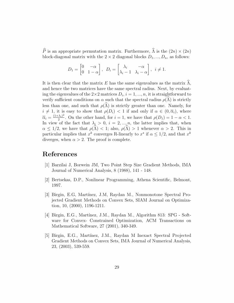
P is an appropriate permutation matrix. Furthermore, Λ is the (2n)× (2n)block-diagonal matrix with the 2× 2 diagonal blocks D1, ..., Dn, as follows:

D1 =

[0 −α0 1− α

], Di =

[λi −α

λi − 1 λi − α

], i 6= 1.

It is then clear that the matrix E has the same eigenvalues as the matrix Λ,and hence the two matrices have the same spectral radius. Next, by evaluat-ing the eigenvalues of the 2×2 matrices Di, i = 1, ..., n, it is straightforward toverify sufficient conditions on α such that the spectral radius ρ(Λ) is strictly

less than one, and such that ρ(Λ) is strictly greater than one. Namely, fori 6= 1, it is easy to show that ρ(Di) < 1 if and only if α ∈ (0, αi), where

αi = (1+λi)2

2. On the other hand, for i = 1, we have that ρ(D1) = 1− α < 1.

In view of the fact that λi > 0, i = 2, ..., n, the latter implies that, whenα ≤ 1/2, we have that ρ(Λ) < 1; also, ρ(Λ) > 1 whenever α > 2. This inparticular implies that xk converges R-linearly to x? if α ≤ 1/2, and that xk

diverges, when α > 2. The proof is complete.

References

[1] Barzilai J, Borwein JM, Two Point Step Size Gradient Methods, IMAJournal of Numerical Analysis, 8 (1988), 141 - 148.

[2] Bertsekas, D.P., Nonlinear Programming, Athena Scientific, Belmont,1997.

[3] Birgin, E.G, Martınez, J.M, Raydan M., Nonmonotone Spectral Pro-jected Gradient Methods on Convex Sets, SIAM Journal on Optimiza-tion, 10, (2000), 1196-1211.

[4] Birgin, E.G., Martınez, J.M., Raydan M., Algorithm 813: SPG - Soft-ware for Convex- Constrained Optimization, ACM Transactions onMathematical Software, 27 (2001), 340-349.

[5] Birgin, E.G., Martınez, J.M., Raydan M Inexact Spectral ProjectedGradient Methods on Convex Sets, IMA Journal of Numerical Analysis,23, (2003), 539-559.

29

[6] Birgin, E.G., Martınez, J.M., Raydan M Spectral Projected Gradi-ent Methods: Review and Perspectives, Journal of Statistical Software60(3), (2014), 1-21.

[7] Boyd, S., Parikh, N., Chu, E., Peleato, B., Eckstein, J., Distributed op-timization and statistical learning via the alternating direction methodof multipliers, Foundations and Trends in Machine Learning, Volume 3,Issue 1, (2011) pp. 1-122.

[8] Cattivelli, F., Sayed, A. H., Diffusion LMS strategies for distributed es-timation, IEEE Transactions on Signal Processing, vol. 58, no. 3, (2010)pp. 1035–1048.

[9] Dai, Y.H., Liao, L.Z., R-Linear Convergence of the Barzilai and BorweinGradient Method, IMA Journal on Numerical Analysis, 22 (2002), 1-10.

[10] Desoer, C., Vidyasagar, M., Feedback Systems: Input-Output Proper-ties, SIAM 2009.

[11] Jakovetic, D., A Unification and Generalization of Exact DistributedFirst Order Methods, arxiv preprint, arXiv:1709.01317, 2017.

[12] P. Di Lorenzo and G. Scutari, Distributed nonconvex optimization overnetworks, in IEEE International Conference on Computational Ad-vances in Multi-Sensor Adaptive Processing (CAMSAP), 2015, pp. 229-232.

[13] Jakovetic, D., Xavier, J., Moura, J. M. F., Fast distributed gradientmethods, IEEE Transactions on Automatic Control, vol. 59, no. 5,(2014) pp. 1131–1146.

[14] Jakovetic, D., Moura, J. M. F., Xavier, J., Distributed Nesterov-likegradient algorithms, in CDC’12, 51st IEEE Conference on Decision andControl, Maui, Hawaii, December 2012, pp. 5459–5464.

[15] Jakovetic, D., Bajovic, D., Krejic, N., Krklec Jerinkic, N., Newton-likeMethod with Diagonal Correction for Distributed Optimization, SIAMJ. Optimization, 27 (2), (2017), 1171-1203.

30

[16] Kar, S., Moura, J. M. F., Ramanan, K., Distributed parameter esti-mation in sensor networks: Nonlinear observation models and imper-fect communication, IEEE Transactions on Information Theory, vol. 58,no. 6, (2012) pp. 3575–3605.

[17] Kar, S., Moura, J. M. F., Distributed Consensus Algorithms in SensorNetworks With Imperfect Communication: Link Failures and ChannelNoise, IEEE Transactions on Signal Processing, vol. 57, no. 1, (2009)pp. 355–369.

[18] Lopes, C., Sayed, A. H., Adaptive estimation algorithms over distributednetworks, in 21st IEICE Signal Processing Symposium, Kyoto, Japan,Nov. 2006.

[19] Mokhtari, A., Ling, Q., Ribeiro, A., Network Newton–Part I: Algorithmand Convergence, 2015, available at: http://arxiv.org/abs/1504.06017

[20] A. Mokhtari, W. Shi, Q. Ling, and A. Ribeiro, DQM: Decentral-ized Quadratically Approximated Alternating Direction Method ofMultipliers, to appear in IEEE Trans. Sig. Process., 2016, DOI:10.1109/TSP.2016.2548989

[21] A. Mokhtari, W. Shi, Q. Ling, and A. Ribeiro, A Decentralized Sec-ond Order Method with Exact Linear Convergence Rate for ConsensusOptimization, 2016, available at: http://arxiv.org/abs/1602.00596

[22] Mota, J., Xavier, J., Aguiar, P., Puschel, M., Distributed optimizationwith local domains: Applications in MPC and network flows, to appearin IEEE Transactions on Automatic Control, 2015.

[23] Nedic, A., Olshevsky, A., Shi, W., Uribe, C.A., Geometrically con-vergent distributed optimization with uncoordinated step-sizes, arXivpreprint, arXiv:1609.05877, 2016.

[24] Nedic, A., Olshevsky, A., Shi, W., Achieving Geometric Convergencefor Distributed Optimization over Time-Varying Graphs, arxiv preprint,arXiv:1607.03218, 2016.

[25] Nedic, A., Ozdaglar, A., Distributed subgradient methods for multi-agent optimization, IEEE Transactions on Automatic Control, vol. 54,no. 1, (2009) pp. 48–61.

31

[26] Qu, G., Li, N., Harnessing smoothness to accelerate distributed opti-mization, IEEE Transactions on Control of Network Systems (to ap-pear)

[27] Raydan, M., On the Barzilai and Borwein Choice of Steplength for theGradient Method, IMA Journal of Numerical Analysis, 13 (1993), 321-326.

[28] Raydan M, Barzilai and Borwein Gradient Method for the Large ScaleUnconstrained Minimization Problem, SIAM Journal on Optimization7 (1997), 26 - 33.

[29] Schizas, I. D. , Ribeiro, A., Giannakis, G. B., Consensus in ad hocWSNs with noisy links – Part I: Distributed estimation of deterministicsignals, IEEE Transactions on Signal Processing, vol. 56, no. 1, (2009)pp. 350–364.

[30] Shi, W., Ling, Q., Wu, G., Yin, W., EXTRA: an Exact First-OrderAlgorithm for Decentralized Consensus Optimization, SIAM Journal onOptimization, No. 25 vol. 2, (2015) pp. 944-966.

[31] J. Xu, S. Zhu, Y. C. Soh, and L. Xie, Augmented distributed gradi-ent methods for multi-agent optimization under uncoordinated constantstep- sizes, in IEEE Conference on Deci- sion and Control (CDC), 2015,pp. 2055-2060.

32