HAL Id: hal-01254856https://hal.archives-ouvertes.fr/hal-01254856

Submitted on 12 Jan 2016

HAL is a multi-disciplinary open accessarchive for the deposit and dissemination of sci-entific research documents, whether they are pub-lished or not. The documents may come fromteaching and research institutions in France orabroad, or from public or private research centers.

L’archive ouverte pluridisciplinaire HAL, estdestinée au dépôt et à la diffusion de documentsscientifiques de niveau recherche, publiés ou non,émanant des établissements d’enseignement et derecherche français ou étrangers, des laboratoirespublics ou privés.

Exact Sparse Approximation Problems viaMixed-Integer Programming: Formulations and

Computational PerformanceSébastien Bourguignon, Jordan Ninin, Hervé Carfantan, Marcel Mongeau

To cite this version:Sébastien Bourguignon, Jordan Ninin, Hervé Carfantan, Marcel Mongeau. Exact Sparse Approxi-mation Problems via Mixed-Integer Programming: Formulations and Computational Performance.IEEE Transactions on Signal Processing, Institute of Electrical and Electronics Engineers, 2016, 64(6), pp.1405-1419. �10.1109/TSP.2015.2496367�. �hal-01254856�

1

Exact Sparse Approximation Problems viaMixed-Integer Programming: Formulations and

Computational PerformanceSebastien Bourguignon, Jordan Ninin, Herve Carfantan, and Marcel Mongeau, Member, IEEE

Abstract—Sparse approximation addresses the problem ofapproximately fitting a linear model with a solution having as fewnon-zero components as possible. While most sparse estimationalgorithms rely on suboptimal formulations, this work studies theperformance of exact optimization of `0-norm-based problemsthrough Mixed-Integer Programs (MIPs). Nine different sparseoptimization problems are formulated based on `1, `2 or `∞data misfit measures, and involving whether constrained orpenalized formulations. For each problem, MIP reformulationsallow exact optimization, with optimality proof, for moderate-sizeyet difficult sparse estimation problems. Algorithmic efficiency ofall formulations is evaluated on sparse deconvolution problems.This study promotes error-constrained minimization of the `0norm as the most efficient choice when associated with `1 and`∞ misfits, while the `2 misfit is more efficiently optimizedwith sparsity-constrained and sparsity-penalized problems. Then,exact `0-norm optimization is shown to outperform classicalmethods in terms of solution quality, both for over- and under-determined problems. Finally, numerical simulations emphasizethe relevance of the different `p fitting possibilities as a functionof the noise statistical distribution. Such exact approaches areshown to be an efficient alternative, in moderate dimension,to classical (suboptimal) sparse approximation algorithms with`2 data misfit. They also provide an algorithmic solution toless common sparse optimization problems based on `1 and`∞ misfits. For each formulation, simulated test problems areproposed where optima have been successfully computed. Dataand optimal solutions are made available as potential benchmarksfor evaluating other sparse approximation methods.

Index Terms—sparse approximation, `0-norm-based problems,optimization, mixed-integer programming, deconvolution

I. INTRODUCTION

A. Sparse estimation for inverse problems

The problem of sparse representation of data y ∈ RN ina dictionary H ∈ RN × RQ consists in finding a solutionx ∈ RQ to the system y = Hx with the fewest non-zerocomponents, i.e., with the lowest sparsity level. In sparseapproximation, in order to account for noise and model errors,the equality constraint is relaxed through the minimizationof the data misfit measure ‖y −Hx‖, where ‖·‖ generallystands for the standard Euclidean norm in RN . Such sparsestrepresentation and approximation problems are essentiallycombinatorial. Finding the best K-sparse solution (the so-lution with K non-zero components) is usually considered

This work was partially supported by the French Groupement de RechercheISIS (Information, Signal, Image, viSion) through its “young researchers”program. One of the authors of this work has been supported by FrenchNational Research Agency (ANR) through JCJC program (project ATOMICn◦ANR 12-JS02-009-01).

too difficult in practical large-scale instances. Indeed, thebrute-force approach that amounts to exploring all the

(QK

)possible combinations, is computationally prohibitive. In theabundant literature on sparse approximation, much work hasbeen dedicated to the relaxation approach that replaces the `0-“norm” sparsity measure, ‖x‖0 := Card{i |xi 6= 0}, with the`1 norm ‖x‖1 :=

∑i |xi|. Many specific convex optimization

algorithms have been proposed in the past decade, see forexample [1], [2]. In addition, conditions were establishedfor which both the `0 and the relaxed `1 problems yieldthe same solution support (the set of non-zero components).These mostly rely on a low sparsity level assumption andon structural hypotheses on the matrix H, such as lowcorrelation of its columns (see [1] and references therein).Alternatively, greedy algorithms build a sparse solution byiteratively adding non-zero components to an initially empty-support solution [3], [4], [5]. More complex forward-backwardmethods [6], [7] may show better performance in practice butwith higher computation time. Tree-search-based methods alsotry to improve the classical greedy algorithms using heuristicsto reduce the complexity of exhaustive combinatorial explo-ration (see e.g., [8] and references therein). Other supportexploration strategies maintain the desired sparsity level ateach iteration, and perform local combinatorial explorationsteps [9]. Optimality proofs for all such strategies also relyon very restrictive hypotheses [10], [11]. More “`0-oriented”approaches were proposed, e.g., by successive continuousapproximations of the `0 norm [12], by descent-based IterativeHard Thresholding (IHT) [13], [14] and by penalty decompo-sition methods [15]. However, without additional assumptionson H, one can only prove that the solution found is a localminimum of the optimization problem. Moreover, for IHT,optimality conditions suffer from the same restrictions as theaforementioned greedy methods [13], [14].

In many inverse problems, the model y ' Hx resultsfrom the discretization of an intrinsically continuous physicalmodel. A typical example is sparse deconvolution, where Hxmodels the convolution of a spike train (in one-dimensionalsignals) or of point sources (in imaging problems) by theimpulse response of the acquisition device [7], [16], [17]. Asimilar problem concerns nonlinear parameter identification,where parameters are discretized on arbitrarily thin grids [7],[18], [19] and estimation amounts to finding a sparse solutionto a linear problem of high dimension. In such cases, thecolumns of H can be highly correlated, so no optimality guar-anty can be obtained for greedy and `1-norm-based methods.

2

Similar problems also arise for variable selection in machinelearning and statistics [6], where the set of features (thecolumns of H) is not designed to satisfy any recovery property.

The aforementioned problems essentially focus on the cor-rect estimation of the support of x. In deconvolution, forexample, support identification corresponds to detection andlocalization of the sources. Since the true sparsity measureis indeed the `0 norm, a global optimum of `0-based for-mulations is more likely to yield exact support identificationthan approximate solutions. Consequently, our interest focuseson optimization methods for `0-norm-based criteria provid-ing optimality guarantees. Such exact approaches are usuallydiscarded, based on the argument that sparse optimizationproblems are NP hard [20]. It is also commonly consideredthat exact optimization amounts to combinatorial explorationof all possible supports, which is nothing but a worst-case-scenario argument. Note however that, in order to reduce thenumber of explored supports, Tropp and Wright [1] mentionedthe possible use of cutting-plane methods, which are one ofthe basic elements of resolution of the mixed-integer programsexplored in the present paper.

Here, we focus on sparse optimization occurring in certaininverse problems with moderate size yet with a complexity suf-ficient to make the usual methods fail in estimating the sparsestsolutions. Examples include spike-train deconvolution in ultra-sonic nondestructive testing (NDT) [16] or Geophysics [17],sparse hyperspectral unmixing [21], and spectral analysis withshort data sets [22]. A first objective of this contribution isto show the viability of exact resolution approaches for suchproblems.

B. Global optimization via Mixed-Integer Programming

We focus on Mixed-Integer Programs (MIP), that is, op-timization problems involving both continuous and integervariables. Such problems are well suited to `0-norm-basedoptimization, since the `0 norm naturally introduces a binarydecision variable for each component (zero or non-zero?).In this paper, MIP refers to the minimization of linear orquadratic criteria subject to linear or quadratic inequalityconstraints. It is commonly claimed that, in the past fifteenyears, a factor 109 was gained in the required computing timefor solving such problems. This gain is due in (roughly) equalparts to (i) hardware improvement, (ii) progress in the resolu-tion of linear programs, and (iii) implementation efficiency ofadvanced mathematical techniques [23]. Therefore, as it willbe shown in this paper, some exact approaches can now beadvantageously used to address the moderate-size, yet difficult,applications enumerated at the end of Section I-A.

To our knowledge, the first MIP reformulation of a sparseoptimization problem is proposed in [24]. However, the au-thors argue that the assumption that |x| is upper bounded,which is required for the MIP reformulation, leads to com-putational inefficiency. Therefore, they choose to consideronly a related problem: the maximum feasible subsystemproblem, for which exact solutions can be found only forvery small instances (N = 16, Q = 32) and no result isgiven concerning the MIP approach. A similar formulation

with binary variables appears in [25], but binary variables arereplaced by continuous variables in [0, 1] in order to yielda convex problem, which is obviously not equivalent to theoriginal one. In [26], some exact and approximate reformula-tions of `0-based problems are surveyed. The authors deplorethe inherent combinatorial difficulty of such MIP problemsbut no practical result is provided. Finally, in [27], noise-free sparse representation problems are formulated as MIP.Here, we address the noisy case, which opens perspectives todifferent possible formulations of the optimization problem.Establishing MIP reformulations for such problems, studyingtheir computational efficiency, investigating properties of opti-mal solutions and comparing them with the results of standardmethods are the core of this paper.

C. Objectives of the paper

This paper shows that different possible reformulationsof sparse approximation problems can be tackled by MIPsolvers. Sparse approximation is intrinsically a bi-objectiveoptimization problem, where both the sparsity measure andthe data misfit measure are optimized. In inverse problems, itis usually formulated through the optimization of a weightedsum of the two terms. However, constrained formulations(involving one criterion to be minimized and the other subjectto a constraint) may also be well suited to MIP reformulations,which are constrained programs by nature. Therefore, westudy the efficiency of MIP solving techniques applied to thefollowing three formulations:

• minimize the `0 norm under a bounded-data-misfit con-straint,

• minimize the data misfit under an `0-boundedness con-straint,

• minimize a weighted sum of the two criteria.

Additionally, we also consider non-quadratic data misfit mea-sures, which may be appropriate if the error term y −Hx isnon-Gaussian. Moreover, piecewise-linear alternatives to the`2 norm ‖x‖2 :=

√∑i |xi|2, may also prove to be more

attractive computationally, because MIPs essentially rely onthe resolution of linear subproblems. In particular, the `1and `∞ (‖x‖∞ := maxi |xi|) norms are easily linearized;formulations based on those norms naturally boil down tooptimization problems involving linear inequality constraintsor linear objective functions. Therefore, we also considerformulations involving `1 and `∞ misfits, for which muchfewer algorithms have been proposed.

Our work establishes MIP reformulations of nine differentsparse approximation problems, which are all evaluated interms of computational efficiency, depending on the sparsitylevel and on the noise level. Then, these formulations arecompared in their ability to identify the exact support inthe presence of noise, depending on the noise statisticaldistribution. Our experimental results additionally show thatthe classical methods are far from reaching acceptable resultsin such cases, whereas the `0-norm formulations do yield moresatisfactory solutions—but with much higher computing time.Note that experiments in both [24] and [27] involve random

3

matrices, which are more likely to satisfy the conditions ensur-ing the optimality of `1-norm-based and greedy approaches. Inmost ill-posed inverse problems, the columns of H are highlycorrelated, so that such conditions certainly do not hold.

The remainder of the paper is organized as follows. Sec-tion II introduces nine optimization formulations of the sparseapproximation problem, and discusses their statistical inter-pretation and the structure of the solution sets. MIP refor-mulations are then established in Section III. Then, basicelements concerning the resolution of MIP problems are givenin Section IV. Experimental results in Section V are dedicatedto the evaluation of computational costs. Section VI comparesthe solutions obtained through MIP optimization with thoseof classical sparse approximation algorithms, on both overde-termined and underdetermined sparse deconvolution problems.Simulations in Section VII evaluate the support identificationperformance of `p-misfit-constrained formulations as a func-tion of p and of the noise statistical distribution. Finally, adiscussion is given in Section VIII.

II. SPARSE OPTIMIZATION PROBLEMS

In sparse approximation, both the sparsity of the solutionand the fidelity of its corresponding data approximation areoptimized. Therefore, the generic sparse approximation prob-lem, which we are interested in, is the following unconstrainedbi-objective optimization problem:

minx

(‖x‖0 , ‖y −Hx‖p), (1)

where p is either 1, 2 or ∞. This section presents nineformulations of this problem and discusses their statisticalinterpretation and the structure of the sets of solutions.

A. Taxonomy

Various mono-objective optimization problems can be for-mulated to address the bi-criterion problem (1). For p ∈{1, 2,∞}, the bounded-error problems read

P0/p : minx‖x‖0 s.t. ‖y −Hx‖p ≤ αp,

and the sparsity-constrained problems read

Pp/0 : minx‖y −Hx‖p s.t. ‖x‖0 ≤ Kp,

where αp and Kp are user-defined threshold parameters.Finally, the penalized problems read

P0+p : minx

µp ‖x‖0 + ‖y −Hx‖pp , for p ∈ {1, 2},and P0+∞ : min

xµ∞ ‖x‖0 + ‖y −Hx‖∞ ,

where µp and µ∞ are user-defined penalty parameters.In this paper, we propose a reformulation of each of these

problems as MIPs. To the best of our knowledge, P0/∞ is theonly sparse approximation problem for which a MIP reformu-lation is mentioned [24]. Remark that the sparse representationcase (noise-free data), which was recently tackled via MIPsin [27] with equality constraint y = Hx, is the special caseof P0/p with αp set to 0, for which P0/1, P0/2, and P0/∞are obviously equivalent. Recall that the sparsity-based inverse

problems considered here are sparse approximation problems:data are always contaminated by measurement noise and themodel may be inexact, so that αp 6= 0.

Choosing one of the nine formulations and the values ofthe parameters (αp, Kp or µp) amounts to selecting someparticular solutions among the wide variety of Pareto-optimalsolutions of problem (1). Note that, for a given `p misfit, noequivalence between the three problems P0/p, Pp/0 and P0+p

can be obtained because the `0 norm is not convex. In par-ticular, solutions in the non-convex part of the Pareto frontiercannot be reached by solving the penalized formulation [28].

B. Statistical interpretations and parameter tuningIn practice, one has to choose one among the nine opti-

mization problems and must set a value for the correspondingparameter. Such choices can be based on statistical arguments.

The `p data-misfit measures, with p ∈ {1, 2,∞}, can beinterpreted in terms of likelihood functions. Let pε be thestatistical distribution of the additive noise term ε = y−Hx.The likelihood function is defined as: L(y;x) := pε(y−Hx).If noise samples εn, n = 1, . . . , N are independent andidentically distributed (i.i.d.) according to a centered Gaussiandistribution, then − logL(y;x) is proportional to ‖y −Hx‖22up to an additive constant. Similarly, − logL(y;x) is pro-portional to ‖y −Hx‖1 (up to an additive constant) if εnare i.i.d. according to a centered Laplace distribution. Sucha heavy-tailed distribution assumption may be appropriate inthe presence of impulsive noise [29], [16]. The `∞ misfit isconnected to an i.i.d. uniform noise distribution assumption.Suppose that ε is uniformly distributed on [−a, a]N , for somegiven a > 0. Then, the likelihood function is constant forany x such that ‖y −Hx‖∞ ≤ a, otherwise it is zero.Consequently, x = argminx ‖y −Hx‖∞ is a maximum-likelihood estimator if noise samples are uniformly distributedon [−a, a], for any a > ‖y −Hx‖∞ [30, Ch. 7.1]. In this case,which arises for example when accounting for quantizationnoise, `∞ data fitting may be a relevant choice—see [31] forboth theoretical and numerical arguments.

Consequently, Pp/0 is a sparsity-constrained maximum like-lihood estimation problem with the aforementioned corre-sponding noise distribution assumption. In a Bayesian setting,P0+p defines a Maximum A Posteriori (MAP) estimate, wherethe `0 term results from a Bernoulli-Gaussian prior modelwith infinite variance Gaussian distribution [7]. Note that,within such a MAP interpretation, solving P0+∞ reducesto solving P0/∞. Indeed, since − logL(y;x) is constant if‖y −Hx‖∞ ≤ a and equals +∞ otherwise, minimizingµ∞ ‖x‖0−logL(y;x) amounts to minimizing ‖x‖0 subject to‖y −Hx‖∞ ≤ a. Finally, P0/p considers a maximal toleranceon the approximation error and cannot be interpreted as amaximum likelihood or MAP estimation problem.

The choice of the formulation also depends on availableprior information about the considered practical problem. Ifreasonable bounds on the acceptable approximation error canbe inferred, e.g., from the knowledge of the signal-to-noiseratio or from a desired approximation quality, then P0/p maybe preferred. In particular, the parameter αp can be fixed ac-cording to the statistics of ‖ε‖p, which can be obtained for any

4

noise distribution (analytically or numerically). If the sparsitylevel is fixed or can be upper bounded, e.g., in a compressioncontext, then Pp/0 may be appropriate. In P0+p, the parameterµp trades off between the noise level and the sparsity level.With the previous MAP interpretation, for p ∈ {1, 2}, it isan explicit function of the noise variance and of the rate ofnon-zero values in the Bernoulli process. Therefore, tuningµp requires more information than tuning the parameters ofthe two other formulations. When too little prior informationis available, a practical solution consists in computing opti-mal solutions corresponding to different parameter tunings—whatever the considered formulation—and then selecting aposteriori the most appropriate one, according to some expertsupervision or to model order selection criteria [32].

C. Structure of the solution sets

We investigate hereafter the structure of the solution sets ofthe different problems, for fixed values of the correspondingparameters αp, Kp and µp. In the following, an optimalsupport refers to a set of indices which supports at least oneoptimal solution. The `0 norm is a piecewise constant function,where each value is attained on a finite number of supports.Hence, for any problem P defined in Section II-A, the setof minimizers can be defined as the finite union of sets ofminimizers on each optimal support: if S denotes the set ofoptimal supports, then:

Arg P =⋃s∈S

Arg Ps,

where Ps denotes the restriction of problem P to the support s.Let us characterize the solution set of Ps. We assume that

the sparsity level of all solutions is lower than N and thatthe matrix H satisfies the Unique Representation Property(URP) [33], that is, any N columns of H are linearly indepen-dent. For any x supported by s, ‖x‖0 is constant, hence Ps

p/0

and Ps0+p are solved by minimizing ‖y −Hsxs‖p, where

xs (respectively, Hs) collects the non-zero components in x(respectively, the corresponding columns of H). Thanks to theURP, Hs has full column rank and, for p = 2, Ps admitsa unique solution (the least-squares solution). Consequently,the solution sets of P2/0 and P0+2 are both (finite) unionsof singletons. The `p norms for p = 1 and p = ∞are not strictly convex, therefore one can only claim thatminxs

‖y −Hsxs‖p is attained on a convex set, such thatHsxs lies in an `p-sphere in dimension Ks − 1, centeredat y. Consequently, for p = 1 and p = ∞, the solutionsets of Pp/0 and P0+p are (finite) unions of convex setsof the form

{‖y −Hsxs‖p = constant

}. Now, consider

the solution set of Ps0/p, which is formed by all vectors

xs such that ‖y −Hsxs‖p ≤ αp. In the particular casewhere minxs

‖y −Hsxs‖p = αp, it comes from the previousarguments that the solution set is a singleton for p = 2,and a convex set for p = 1 and p = ∞. But, in the mostfrequent case where minxs

‖y −Hsxs‖p < αp, the solution

set{xs

∣∣ ‖y −Hsxs‖p ≤ αp

}is such that Hsxs lies in an

`p-ball of dimension Ks, centered at y, and the solution set ofP0/p is a finite union of such sets. Consequently, for a given p,

the solution set of P0/p is generally “larger” than the solutionsets of Pp/0 and P0+p. In particular, the minimizers of theselast two problems may be unique. For example, with someadditional assumptions on the data y and on the matrix H, thesolution of P0+2 is unique [34]. On the contrary, the minimizerof P0/p is certainly not unique, except in very specific cases.

III. MIXED-INTEGER REFORMULATIONS

In this section, we establish the reformulations of opti-mization problems P0/p, Pp/0 and P0+p for p ∈ {1, 2,∞},as Mixed-Integer Linear Programs (MILPs), Mixed-IntegerQuadratic Programs (MIQPs) or Mixed-Integer QuadraticallyConstrained (linear) Programs (MIQCPs).

A. Definitions of MILP, MIQP and MIQCP

The general form of an MILP is

minvcᵀv, subject to (s.t.)

Ainv ≤ bin,

Aeqv = beq,

lb ≤ v ≤ ub,

vj ∈ Z,∀j ∈ I,where v ∈ RJ is the vector of optimization variables; c ∈ RJ

defines the linear objective function; bin ∈ RPin , beq ∈ RPeq ,Ain ∈ RPin × RJ and Aeq ∈ RPeq × RJ define the inequalityand equality constraints; lb and ub ∈ RJ are respectivelythe vectors of lower and upper bounds of the optimizationvariables; I is the index set corresponding to the componentsof v that are constrained to be integer-valued.

An MIQP has the general form:

minv

1

2vᵀFv + cᵀv, s.t.

Ainv ≤ bin,

Aeqv = beq,

lb ≤ v ≤ ub,

vj ∈ Z,∀j ∈ I,where F is a J × J matrix.

Finally, the form of an MIQCP that is of interest in thispaper is:

minvcᵀv, s.t.

1

2vᵀBv + dᵀv ≤ e,

Ainv ≤ bin,

Aeqv = beq,

lb ≤ v ≤ ub,

vj ∈ Z,∀j ∈ I,where B is a J × J matrix, d ∈ RJ and e ∈ R.

B. Equivalent reformulation techniques

We now present standard reformulation techniques thatenables to express each of the nine optimization problemsintroduced in Section II-A as an MILP, an MIQP or an MIQCP,without any approximation.

5

1) Boundedness assumption and “big-M” reformulation ofthe `0 norm: For each q = 1, 2, . . . , Q, let us introduce anadditional binary optimization variable bq, such that

bq = 0⇔ xq = 0. (2)

Then, the non-linear sparsity measure ‖x‖0 is equal to the lin-ear term 1ᵀ

Qb (=∑

q bq), where 1Q is the Q-dimensional all-ones column vector. The logical constraint (2) must howeverbe translated into (in)equality constraints compatible with MIP,ideally through linear constraints. One standard way to achievethis (see e.g. [24], [27]) is to assume that a solution x of theproblem under consideration satisfies the following constraintsfor some sufficiently large pre-defined value M > 0:

−M1Q < x < M1Q. (3)

This assumption supposes that the problem admits boundedoptimal solutions, which is not restrictive in our practicalapplications. The parameter M has to be large enough so that‖x‖∞ < M at any desirable optimal solution x. On the otherhand, the bound M must be as tight as possible in order toimprove computational efficiency; therefore tuning the valueof parameter M may be a critical issue [24]. In the problemsaddressed in this paper, satisfactory results are obtained witha rather simple empirical rule discussed in Section V-B. Notethat specific lower and upper bounds for each component xqcould also be advantageously considered [27] if correspondingprior information is available.

The reformulations of `0-norm-based constraints and objec-tive functions are obtained through the two following respec-tive lemmas.

Lemma 1: Considering the boundedness assumption (3),

‖x‖0 ≤ K ⇔

∃b ∈ {0; 1}Q such that

Q∑q=1

bq ≤ K, (i)

−Mb ≤ x ≤Mb. (ii)

Proof: The ⇒ implication is straightforward by consid-ering b defined by Equation (2). Now, let b ∈ {0; 1}Q satisfy(i) and (ii), and suppose ‖x‖0 > K. From (ii), one has(bq = 0) ⇒ (xq = 0), that is, (xq 6= 0) ⇒ (bq = 1). Hencebq = 1 for at least K + 1 indices q, which contradicts (i).Consequently, ‖x‖0 ≤ K.

Lemma 2: Considering the boundedness assumption (3),

minx∈F‖x‖0 ⇔ min

x∈Fb∈{0,1}Q

Q∑q=1

bq s.t. −Mb ≤ x ≤Mb,

where F represents the feasible domain of the problem underconsideration.

Proof: Similar to that of Lemma 1.Such a reformulation technique is commonly referred to as“big-M” reformulation. Remark finally that another reformu-lation of the cumbersome logical constraint (2) consists inintroducing the equality constraint xq(bq − 1) = 0. However,the latter is a bi-linear constraint, typically less interesting interms of computation time for off-the-self MIP solvers than

linear constraints [35].

2) Reformulation of the `1 data misfit measure: The `1misfit term can be written linearly as ‖y −Hx‖1 =

∑n wn,

with additional constraints wn = |yn − hrnx|, n = 1, . . . , N ,

where hrn denotes the nth row of H. Then, these con-

straints can be relaxed (exactly) by the linear inequalities:−w ≤ y−Hx ≤ w, with column vector w = [w1, . . . , wN ]ᵀ,thanks to the two following lemmas.

Lemma 3: minx∈F‖y −Hx‖1

⇔ minx∈F,w∈RN

∑n

wn s.t. −w ≤ y −Hx ≤ w.

Proof: Let fn(x) = yn − hrnx. The following optimiza-

tion problems are equivalent:

Pa : minx∈F

∑n

|fn(x)|

Pb : minx∈F,w∈RN

∑n

wn s.t. |fn(x)| = wn,∀n

Pc : minx∈F,w∈RN

∑n

wn s.t. |fn(x)| ≤ wn,∀n.

Indeed, Pa ⇔ Pb is trivial. In order to show that Pb ⇔ Pc,one can simply remark that if an optimal solution (x?,w?)of Pc is such that |fn0

(x?)| < w?n0

for some index n0, thenone can straightforwardly construct a better feasible solutionfor Pc, which yields a contradiction.

Lemma 3 will be used to obtain a MIP reformulationof P1/0 and P0+1, which involve the `1-misfit term in theobjective function. For P0/1, which involves the `1-misfit termas a constraint, we use the following lemma:

Lemma 4: Let (x?,w?) solve the optimization problem:

Pd : minx∈RQ,w∈RN

‖x‖0 s.t.

∑n

wn ≤ α1

−w ≤ y −Hx ≤ w.Then, x? is a solution of P0/1.

Proof: Suppose that (x?,w?) solves (Pd) and let w′n :=|y − hr

nx?|, ∀n. Then,

∑n w′n ≤

∑n w

?n ≤ α1 and (x?,w′)

is a solution of:

Pe : minx∈RQ,w∈RN

‖x‖0 s.t.

∑n

wn ≤ α1

|yn − hrnx| = wn,∀n.

Indeed, since Pd is a relaxation of Pe—the feasible set of Pe

is a subset of that of Pd—, its optimal value, ‖x?‖0, is a lowerbound for the optimal value of Pe. The solution (x?,w′) isclearly feasible for Pe and it attains the lower bound ‖x?‖0.Hence, it is optimal for Pe. Finally, Pe is clearly equivalentto P0/1.Let us remark finally that problems Pd and Pe are not strictlyequivalent because they are not minimized by the same coupleof vectors (x,w), but they share the same solution set for x.

3) Reformulation of the `∞ data misfit measure: P0/∞naturally brings linear inequality constraints as

‖y −Hx‖∞ ≤ α∞ ⇔ − α∞1N ≤ y −Hx ≤ α∞1N .

6

For both P∞/0 and P0+∞, involving the `∞ norm in theobjective function, one can simply introduce an additionalscalar variable z such that minimizing ‖y −Hx‖∞ amountsto minimizing z under the constraints

−z1N ≤ y −Hx ≤ z1N .

Here again, one can easily show that an optimal solution ofthe original problem will necessarily satisfy ‖y −Hx‖∞ = z.

C. Mixed-integer programming reformulations

Given the reformulation techniques of Section III-B, thenine problem reformulations proposed in Table I are straight-forward.

IV. MIP RESOLUTION: BASIC ELEMENTS

Mixed-integer programming problems are not easy prob-lems. MILP problems are already NP-hard [36]. As a con-sequence, reducing sparse approximation problems to MILP,MIQP or MIQCP problems does not per se reduce thecomplexity. Nevertheless, such MIP reformulations not onlyopen up possibilities to prove the optimality (or quantify thesub-optimality) of solutions, but also allows one to benefitfrom decades of exponential progress in terms of requiredcomputing time to solve a given MIP problem. This progressdoes not simply reflect the doubling of computing powerevery 18 months, it is also a consequence of fast progress inboth the theory and practice of linear programming and dis-crete optimization (duality, numerical linear algebra, interior-point methods, semi-definite positive relaxations, branch andbound/cut/price methods, decomposition approaches, globaloptimization, etc.) Once the sparse approximation problemis recast as a MIP problem, then state-of-the-art off-the-shelf software can be used, such as BARON, COUENNE,CPLEX, GloMIQO, GUROBI, MOSEK or Xpress-MP—seefor example [35] and references therein. We chose to useCPLEX [23] because it is unanimously considered among thebest MIP solvers. CPLEX has been developed over the lastthirty years and includes the best strategies developed by theMIP community. Moreover, it is freely available for researchand teaching purposes.

The main method behind the CPLEX MIP solver is abranch-and-cut algorithm. Globally, it implements a branch-and-bound strategy (i.e., a tree-structured implicit enumerationalgorithm) based on successive continuous relaxations of theinteger variables [37]. Each branch generates a subproblemby fixing some integer (in our case, binary) variables, and aset of branches is constructed corresponding to the differentpossible configurations of such variables. Then, the aim is todiscard (huge) parts of the remaining combinatorial tree bylower bounding the objective function on the correspondingsubproblems. To obtain such lower bounds, a continuousrelaxation of each subproblem is formed by relaxing theinteger variables. Linear constraints, such as Gomory cuttingplanes [38], are added to each generated (continuous relax-ation) subproblem, so that the continuous solution convergesto an integer solution. Such cutting planes remove part ofthe feasible domain of the subproblem that does not contain

any integer solution. This approach amounts to attemptingto construct the convex hull of the set of integer feasiblesolutions of each subproblem. CPLEX incorporates severaltechniques in order to improve performance, such as constraintpropagation techniques [39], linear algebra techniques [23] andheuristic techniques to find rapidly a good integer solution.Doing so, parts of the research space are eliminated only if itis proved that they do not contain the global minimum.

The best current integer solution provides an upper bound ofthe global minimum of the entire problem. The solution of thecurrent relaxed (continuous) subproblem gives a lower boundof the global minimum of the current subproblem with integerconstraints under consideration. The worst solution of allrelaxed subproblems—the one that achieves the lowest lowerbound—gives a certified lower bound of the global minimumof the entire problem. If such a lower bound is attained bythe best current integer solution, then a global minimizer isfound and optimality is proved. Otherwise, the entire processis iterated by creating new branches. The algorithm convergestowards such a certified optimum in a finite number of steps.If the solver reaches the time limit, the duality gap (thedifference between the best solution found and the certifiedlower bound of the global minimum) provides a measure ofsub-optimality of the solution found. Note that tree-searchbased greedy algorithms such as in [8] also rely on tree-based (local) exploration and on lower-bounding the objectivefunction on sets of solutions, which is used inside a greedyprocedure. Therefore, they do not come with any optimalityguarantee.

Remark that in most sparsity-inspired signal processingproblems, the matrix H satisfies specific properties that areexploited for efficient computations. In particular, if H rep-resents a redundant set of transforms based on multi-scalerepresentations such as wavelets [40], matrix-vector productsHv and Hᵀv (where v is some given vector of an appropriatedimension) can be computed by fast algorithms using FastFourier Transforms (FFT). In 1D (respectively, 2D) deconvo-lution problems, H is a Toeplitz (respectively, Toeplitz-block-Toeplitz) matrix, so that matrix-vector products can also becomputed by FFT. No such matrix structure is exploited withinthe standard mixed-integer optimization algorithms, as they areimplemented as general-purpose MIP solvers. The only matrixproperty that is exploited here is the possible sparsity of thematrix H to compute fast vector products. This is particularlythe case for the finite impulse response (FIR) deconvolutionproblems that are considered hereafter.

V. EXPERIMENTAL RESULTS: OPTIMIZATIONPERFORMANCE

This section presents the test problems and the computa-tional framework. Then, the computational efficiency of thenine MIP reformulations is studied.

A. Definition of test problems

The different MIP reformulations are evaluated on one-dimensional sparse deconvolution problems. Such problemsare typically encountered for example in ultrasonic NDT [16]

7

Problem Equivalent MIP reformulation MIP classBounded-misfit formulations (parameters: α2, α1 and α∞)

P0/2 minx∈RQ,b∈{0,1}Q

1ᵀQb s.t.

{xᵀHᵀHx− 2yᵀHx ≤ α2

2 − yᵀy

−Mb ≤ x ≤Mb MIQCP

P0/1 minx∈RQ,b∈{0,1}Q,w∈RN

1ᵀQb s.t.

1ᵀNw ≤ α1

−w ≤ y −Hx ≤ w−Mb ≤ x ≤Mb

MILP

P0/∞ minx∈RQ,b∈{0,1}Q

1ᵀQb s.t.

{−α∞1N ≤ y −Hx ≤ α∞1N

−Mb ≤ x ≤Mb MILP

Sparsity-constrained formulations (parameters: K2, K1 and K∞)

P2/0 minx∈RQ,b∈{0,1}Q

xᵀHᵀHx− 2yᵀHx s.t.

{1ᵀQb ≤ K2

−Mb ≤ x ≤MbMIQP

P1/0 minx∈RQ,b∈{0,1}Q,w∈RN

1ᵀNw s.t.

1ᵀQb ≤ K1

−w ≤ y −Hx ≤ w−Mb ≤ x ≤Mb

MILP

P∞/0 minx∈RQ,b∈{0,1}Q,z∈R

z s.t.

1ᵀQb ≤ K∞

−z1N ≤ y −Hx ≤ z1N

−Mb ≤ x ≤MbMILP

Penalized formulations (parameters: µ2, µ1 and µ∞)P0+2 min

x∈RQ,b∈{0,1}Qµ21

ᵀQb+ x

ᵀHᵀHx− 2yᵀHx s.t.{−Mb ≤ x ≤Mb MIQP

P0+1 minx∈RQ,b∈{0,1}Q,w∈RN

µ11ᵀQb+ 1N

ᵀw s.t.

{−w ≤ y −Hx ≤ w−Mb ≤ x ≤Mb MILP

P0+∞ minx∈RQ,b∈{0,1}Q,z∈R

µ∞1ᵀQb+ z s.t.

{−z1N ≤ y −Hx ≤ z1N

−Mb ≤ x ≤Mb MILP

TABLE IMIXED-INTEGER PROGRAMMING REFORMULATIONS OF NINE SPARSE APPROXIMATION PROBLEMS.

and in seismic reflection in Geophysics [17]. In the following,x is a K-sparse sequence in R100 (i.e., Q = 100), withuniformly distributed spike locations, where the sparsity level,K, is varying. In order to avoid arbitrary small spike values,each non-zero amplitude is drawn as sign(u) + u, whereu is a centered Gaussian sample with unit variance. Thematrix H is the discrete convolution matrix correspondingto the 21-sample impulse response shown in Fig. 1 (left).With the boundary assumption that x is zero outside itsdomain, y is a 120-sample signal (i.e., N = 120). Whitenoise is added with variable signal-to-noise ratio (SNR). In thissection, noise samples are generated according to a centerednormal distribution N (0, σ2), with σ such that SNRdB =

10 log10

(‖Hx‖22/(Nσ2)

). We name such problems SASNR

K .Note that they are slightly overdetermined (Q < N ), whereastypical sparse approximation problems deal with largely under-determined systems. However, trivial inversion is not satisfac-

tory here, because of the presence of noise and of the ill-conditioned nature of H (cond(H) ' 103).

We consider problems SASNRK with K varying between 5

and 11, and SNR varying from +∞ (noise-free data) downto10 dB. One example of data is given in Fig. 1 (right) for K = 7and SNR = 20 dB. It illustrates the difficulty of sparse decon-volution problems arising for example in ultrasonic NDT [16].The oscillating impulse response and the proximity of thespikes produce overlapping echoes in the available data. As theechoes cannot be distinguished visually, numerical techniquesare required. All data and optimization results of this sectionare available online as supplementary multimedia material.

B. Machine configuration and implementation details

Optimization is run with IBM ILOG CPLEX V12.6.0 from aMatlab interface on a computer with eight Intel Xeon X5472processors with Central Processing Units (CPU) clocked at

8

−10 0 10

−0.5

0

0.5

1

0 20 40 60 80 100 120

−2

0

2

Fig. 1. Example of sparse deconvolution data. Left: impulse response. Right:7-sparse sequence x (circles) and noisy convolved data y, with SNR = 20 dB.

3 GHz. The maximum time allowed for each resolution isset to Tmax = 1000s. The other CPLEX parameters are setto their default value. For each problem, the “big-M” con-stant is set to M = 1.1x1max, where x1max := ‖Hᵀy‖∞/‖h‖

22

corresponds to the maximum amplitude of 1-sparse solutionsestimated by least-squares. If the boundedness assumption (3)is saturated—i.e., one component in the solution x reaches thevalue −M or M—then the optimization is successively runagain with M replaced with 1.1M , until the obtained solutionsatisfies ‖x‖∞ < M . The CPU times given below includesuch restarts. With this heuristic strategy, in our simulations,only few cases led to such saturation: no restart was necessaryin 90 % of the cases, and the average number of restarts inthe other cases was approximately 1.6.

C. Evaluation of computational costs

Each of the nine MIP reformulations of Table I is runfor fifty random instances (for both spike distributions andnoise realizations) of each SASNR

K problem. In this section, inorder to ensure a fair comparison (in terms of computationalefficiency), the parameters Kp are set to the true sparsitylevel K, and parameters αp and µp are set by trial and error,until the sparsity level of each solution equals K. Note thatin our case, the matrix H has full column rank, hence `0inequality constraints in Pp/0 will yield the same results asif they were equality constraints. That is, when imposing‖x‖0 ≤ K, all the K columns of matrix H contributeto the reduction of the data misfit. However, formulationswith inequality constraints yielded lower computing times.Sparse representation problems (noise-free data, SNR = ∞)are addressed through P0/p for p ∈ {1, 2,∞}, with thresholdαp = 10−8. Remark that in the noise-free case, no sparsity-enhancing algorithm is indeed necessary, since the solutioncan simply be computed by least squares.

Average CPU times obtained for MIP reformulations aregiven in Table II. The figures on the left-hand side of eachcolumn is the time required to prove the global optimality ofthe solution found. The figures on the right-hand side indicatethe time after which the support of the solution was found,which is generally much lower. The figures in parenthesesindicate the number of instances for which optimality was notproved within 1000s.

All CPU times increase with the sparsity level K, but alsowith the noise level. In particular, for SNR = 10 dB andK = 11, for each formulation, optimality of the solutionswas obtained in less than 1000s only on a fraction of the fiftyinstances. In order to explain such behavior, let us remark thatthe sparsity level (respectively, the noise level) increases thesize of the feasible domain of Pp/0 (respectively, of P0/p).

More generally, for all problems, if either the sparsity level orthe noise level increases, then the branch-and-bound strategybecomes less efficient in discriminating between concurrentcandidates and in eliminating some of them.

With SNR = 30 dB, the lowest CPU times are achievedby solving P0+2—although optimization did not terminatewithin 1000s for one instance of SA30

11. When the noiselevel increases, solving P0/1 and P0/∞ problems becomesmore efficient computationally, and their superiority over otherproblems increases with both the sparsity level and the noiselevel. In particular, P0/1 problems were always solved exactlyin less than 1000s, except for (SNR = 20 dB, K = 11). Resultsare slightly not as good for P0/∞, where optimization did notterminate within 1000s for three more instances with SNR =20 dB and K = 11. Note that even a small amount of noiseseverely degrades the resolution performance of problemsP0/p. Optimization of P0/2, the only problem with a quadraticconstraint, is the most time-consuming among all proposedformulations. Non-linear constraints are known to make theMIP really difficult to solve [35]. An element of explanationcan be found by comparing the Lagrangians of formulationsinvolving `2 misfits. Indeed, the Lagrangian of P0/2 containstrilinear terms. On the contrary, the Lagrangians of P2/0 andof P0+2 are quadratic functions. Therefore, optimizing a linearfunction under quadratic constraints is more complex thanoptimizing a quadratic function under linear constraints.

For any p ∈ {1, 2,∞}, solving problems P0+p generallyperforms better than solving problems Pp/0 at high SNR. Onthe contrary, as the noise level increases, sparsity-constrainedformulations outperform penalized versions. For both formu-lations, which involve the data misfit in the objective function,using an `2 misfit measure is the most efficient choice, andboth `1- and `∞-misfit optimizations behave similarly.

We also note a high dispersion of the required CPU timesamong the fifty realizations of each problem. For example,the average time for the resolution of P0+1 on SA20

9 prob-lems was approximately 11s on forty-eight instances, whereasoptimization did not terminate after 1000s on the two otherinstances. We also remark that, for P0/2, optimality was notproved within 1000s for two instances of the simplest testproblem SA+∞

5 . Two other instances of SA+∞5 also required

a much higher CPU time than the others, which leads to anatypically high average time of 53s, reflecting once again thedifficulty of the quadratically-constrained problem P0/2.

Finally, let us evaluate the CPU time of exhaustive com-binatorial exploration for P2/0. Using notations introducedin Section II-C, for a given support s with K components,the minimizer of Ps

2/0 has the closed-form expression xs =

(HsᵀHs)

−1Hs

ᵀy. Then, the least-squares misfit value iscomputed by: ‖y −Hsxs‖2 = ‖y‖2 − ‖Hsxs‖2. In practice,xs can be computed by performing Cholesky decompositionof Hs

ᵀHs, so that one computation of the objective functionmainly amounts to two K × K triangular inversions. TheCPU time, denoted cK , of one such computation is estimatedby averaging over 105 inversions. Then, neglecting the costof Cholesky factorizations, the cost for testing all K-sparsesolutions is extrapolated as

(QK

)cK . It yields approximately

9

Error-constrained problems Sparsity-constrained problems Penalized problemsP0/2 P0/1 P0/∞ P2/0 P1/0 P∞/0 P0+2 P0+1 P0+∞

SNR = ∞K = 5 53 |50 (2) 0.07|0.03 0.06|0.03K = 7 3.8 |3.6 0.09|0.03 0.08|0.03K = 9 4.4 |4.2 0.12|0.03 0.10|0.03

K = 11 5.2 |5.0 0.14|0.03 0.13|0.03SNR = 30 dB

K = 5 13 |7.2 0.3 | 0.2 0.1 | 0.1 0.3 |0.2 0.5 |0.4 0.5 |0.4 0.2 |0.1 0.4 |0.2 0.4 |0.2K = 7 17 |6.7 1.4 | 0.4 0.3 | 0.1 0.5 |0.3 1.4 |0.8 1.4 |1.0 0.4 |0.2 1.0 |0.6 0.8 |0.4K = 9 132|37 3.1 | 1.0 1.7 | 0.5 3.0 |1.0 9.3 |3.0 25 |7.5 1.9 |0.8(1) 19 |2.7 17 |2.7

K = 11 399|96 (18) 18 | 4.1 19 | 2.1 29 |4.0(1) 72 |11 (2) 78 | 17 (9) 11 |2.7(1) 60 |13 (1) 48 | 14 (4)

SNR = 20 dBK = 5 13 |8.6 0.3 | 0.2 0.1 | 0.1 0.3 |0.2 0.6 |0.3 0.5 |0.4 0.3 |0.2 0.6 |0.3 0.4 |0.2K = 7 48 |11 (1) 1.0 | 0.4 0.5 | 0.1 1.3 |0.6 4.0 |1.8 4.2 |3.5 6.6 |0.9 14 |1.5(1) 29 | 14K = 9 285|82 (9) 6.6 | 2.7 3.7 | 0.4 18 |3.4(1) 30 |6.4(1) 72 | 64 (2) 28 |13 (2) 11 |2.8(2) 87 | 18 (2)

K = 11 - | - (50) 67 | 16 65 | 11 (3) 166|21 (6) 244|22 (11) 355|260(20) 104|16 (5) 179|58 (13) 299| 38 (17)

SNR = 10 dBK = 5 20 |4.9 0.5 | 0.2 0.2 | 0.1 0.4 |0.2 1.3 |0.6 1.7 |1.4 1.9 |1.7 2.0 |0.5(2) 15 |0.8K = 7 195|27 (2) 2.3 | 0.6 1.4 | 0.2 3.5 |0.7 11 |3.0 40 | 39 42 |2.4 73 |4.0(3) 66 | 15 (6)

K = 9 485|63 (34) 24 | 3.9 26 | 1.2 54 |12 (1) 189|28 (4) 220|218(11) 96 |25 (11) 230|11 (18) 215| 32 (16)

K = 11 - | - (50) 287 | 44 (12) 211 | 9.0 (9) 358|26 (24) 670|75 (42) 600|598(39) 340|34 (32) 300|13 (43) 508|101(44)

TABLE IICPU TIMES (IN SECONDS) OBTAINED BY THE NINE MIP REFORMULATIONS, AS A FUNCTION OF THE SIGNAL-TO-NOISE RATIO (SNR) AND OF THE

SPARSITY LEVEL (K), AVERAGED OVER 50 INSTANCES OF EACH PROBLEM. THE FIRST NUMBER INDICATES THE CPU TIME FOR ESTABLISHINGOPTIMALITY OF THE SOLUTION. THE SECOND NUMBER GIVES THE CPU TIME AT WHICH THE CORRESPONDING OPTIMUM WAS FOUND. NUMBERS IN

PARENTHESES COUNT THE INSTANCES FOR WHICH OPTIMALITY WAS NOT PROVEN IN LESS THAN 1000S. FOR REFERENCE, THE COMPUTATION TIME OFCLASSICAL SPARSE APPROXIMATION ALGORITHMS ON OUR HARDWARE CAN BE FOUND IN FIG. 2.

1500s for K = 5, 4 days for K = 7, and more thanone year for K = 9. Problems based on both `1 and`∞ misfits require the resolution of a linear program foreach support, therefore the corresponding exhaustive searchyields still higher computational costs than in the `2 case.Consequently, exhaustive search cannot be considered as apractical solution, even for such moderate-size problems. Inorder to emphasize the ability of the MIP solver to removeimportant parts of the full combinatorial tree search, we givea last indicator. For P2/0 with SNR = 30 dB and K = 9,for which all instances were successfully solved, the averagenumber of combinations that were explicitly considered in thebranch-and-bound procedure is about 4.5 105, to be comparedwith the total number of

(1009

)' 1.9 1012 combinations.

VI. EXPERIMENTAL RESULTS: EVALUATION OF SOLUTIONS

We now compare the solutions obtained via MIP optimiza-tion with those of classical sparse approximation methods:Orthogonal Matching Pursuit (OMP) [5], Single Best Re-placement (SBR) [7], Iterative Hard Thresholding (IHT)1 [13],[14] and the minimization of the `1-norm-penalized least-squares criterion (`1-relax) using homotopy continuation [41].All algorithms are tuned so that all solutions have the correctnumber of spikes. Therefore, all methods are put in a favorablesetting for evaluating their ability to retrieve the correct supportof the solution.

Recall that for sparse deconvolution, none of the clas-sical methods are theoretically guaranteed to solve the `0-norm problem. As seen in the previous section, the MIP

1We used T. Blumensath’s implementation of IHT (program AIHT.m)available at: http://www.personal.soton.ac.uk/tb1m08/sparsify/sparsify.html

approach can compute an exact solution, but requires a largercomputation time. In order to evaluate intermediate solutionsfound by the MIP solver, we consider several values of themaximum time allowed for each MIP resolution: Tmax =1s,10s, 100s and 1000s. If the maximum time is reached, thenthe current solution is considered—which is the best solutionfound, without any optimality guarantee. The parameter M istuned as explained in Section V-B when running optimizationwith Tmax = 1000s. Then, this value is also used for lowervalues of Tmax.

In this section, we consider two types of sparse deconvo-lution problems. The first problems are similar to those ofSection V-A, with N = 120 and Q = 100, and are thereforeslightly overdetermined. The second ones are underdeterminedproblems, the most frequent case in sparse approximation.Such problems may arise in high resolution sparse deconvolu-tion. Indeed, the true spike locations are generally continuous-valued (e.g., representing times of flight of reflected waves),and the model Hx is a discrete approximation of a continuousintegral equation. The discretization step is usually chosenequal to the sampling period of the data, thus H is a discreteconvolution matrix. Such a choice may be too rough and canlead to erroneous spike locations [42]. In order to improve themodel, one may consider an upsampled convolution model,where both the impulse response and the sparse sequence areupsampled by an integer factor, UF. Then, H can be viewed asthe concatenation of UF discrete convolution matrices. Detailabout the corresponding matrix structure can be found in [42].In the following, we consider UF = 2, so that N = 120and Q = 200. Recall however that the intrinsic difficultyof sparse deconvolution is mostly due to the ill-conditioned

10

nature of matrix H and to the presence of noise, even in theoverdetermined case.

Fifty random instances are run with UF = 1 and UF = 2,SNR = ∞ and SNR = 20 dB, and sparsity levels K varyingbetween 5 and 11. In the noise-free case, for the MIP ap-proach, only P0/p problems are relevant. Therefore, solutionsare computed via the optimization of P0/∞ (with thresholdα∞ = 10−8), which was the most efficient computationally(see Section V-C). All data and MIP optimization results ofthis section are available online as supplementary multimediamaterial.

In the noisy case, we consider P2/0, since the classicalmethods rely on `2 data misfit measures. Two quality indicesare computed for each simulated data set:• the exact recovery rate, which is the average number of

simulations for which a given algorithm correctly locatesthe support of the true sequence;

• the average spike distance between the estimated and thetrue sequences. To this aim, a distance similar to thatused in neuroscience [43] is defined: both estimated andtrue spike trains are convolved with a continuous-domainGaussian kernel (with standard deviation chosen equalto the discretization step of the spikes). Then, the `2-norm error between both signals is computed. Such acriterion is less severe than the exact recovery rate if theestimated spikes are slightly shifted with respect to thetrue ones, and also gives more importance to spikes withhigh amplitudes.

Note that with SNR = ∞, the true sequence is a minimizerof P0/p, with p = 1, 2,∞. Hence the expected exact recoveryrate for the MIP approach is 100%. On the other hand, in thenoisy case, the minimizer of P2/0 may not be obtained on thetrue support. Therefore, successful global optimization doesnot always produce exact recovery.

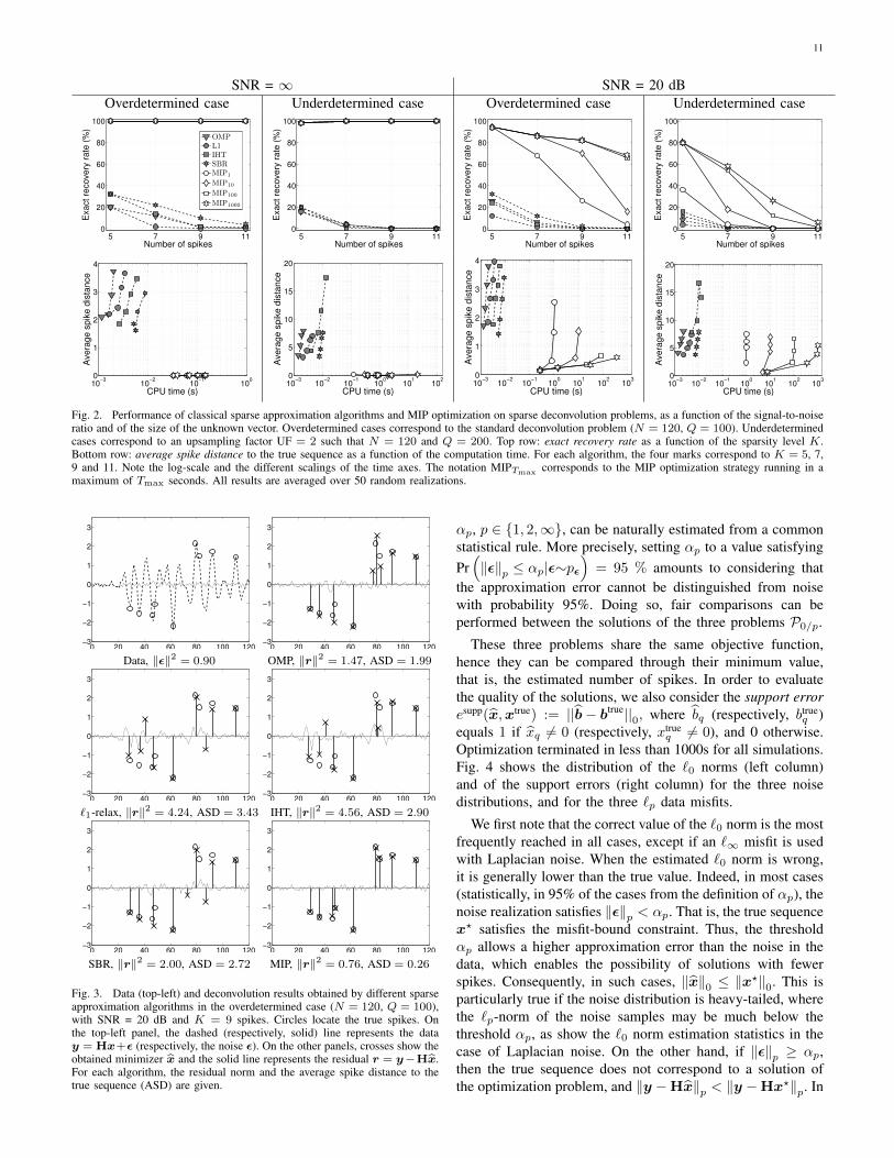
Results are summarized in Fig. 2. The top row shows theaverage exact recovery rate as a function of the number ofspikes, and the bottom row plots the average spike distance tothe true sequence as a function of the CPU time.

Let us first focus on the noise-free case (left columns).Recall that, in the overdetermined noise-free case, the solutioncan simply be computed by least squares. Simulations are stillof interest, however, in order to compare the algorithms inan ideal and simple context. For all classical algorithms, theexact recovery rate is lower than 40% in the overdeterminedcase, and decreases as the sparsity level increases (top row).Their performance is still worse in the underdetermined case,where the exact recovery rate is close to zero, except for thesimplest problems (K=5). Their average spike distance to thetrue sequence (bottom row) is logically lower for algorithmsrequiring more computation time. We note in particular thebad results obtained by IHT in the underdetermined case. Suchbad performance of IHT was already attested when theoreticaloptimality conditions do not hold [14]. This is particularlytrue in the underdetermined case, where the columns of Hare strongly correlated. On the contrary, the MIP strategycorrectly retrieves the support in nearly 100% of the noise-free instances, even with the computation time limited to1s. Actually, only one instance led to erroneous support

identification (for UF = 2 and K = 5), meaning that thesolution was not found, even within 1000s. The MIP approachalso gives an average spike distance close to zero, which meansthat both the supports and the amplitudes of the solutions havebeen correctly recovered, even in the underdetermined case,but with a larger computation time (from 0.03s to 0.2s forUF = 1, and from 0.1s to 20s for UF = 2). Note however thatall classical algorithms are still much faster on such relativelysmall problems (between 10−3s and 10−2s).

In the more realistic noisy case (SNR = 20 dB), the resultsof the classical algorithms are very similar to those obtainedin the noise-free case, both in terms of exact recovery rate,average spike distance and CPU time. In contrast, the MIPperformance deteriorates, and the exact recovery rate quicklydecreases as the number of spikes increases. Recall howeverthat, in the presence of noise, the minimizer of P2/0 maynot retrieve the correct support: in the overdetermined case,for example, the MIP solver returns the optimal solution inless than 1000s in 94% of the instances, whereas the averageexact recovery rate is much lower. However, it is still betterthan that of the classical methods with Tmax = 1s, andeven much better if Tmax is increased to 100s or 1000s. TheMIP approach also outperforms classical methods in terms ofaverage spike distance, in particular if Tmax is high enough. Inthe overdetermined case, the average computing time rangesfrom 0.25s (for K = 5) to 350s (for K = 11) and, asmentioned earlier, global optimality was obtained in less than1000s for most simulations. In the underdetermined case,however, an optimum was not proved to be found within 1000sin 51 % of the instances, that mostly correspond to the caseswhere K = 9 and K = 11. This analysis corroborates theresults in Section V-C: the presence of noise strongly impactsthe computing time of the MIP solver, and therefore the qualityof the solutions obtained by early stopping.

A typical data set and estimated sparse sequences are shownin Fig. 3. It corresponds to the overdetermined case, the truesequence is 9-sparse and SNR = 20 dB. In this example, theMIP approach is the only algorithm that correctly identifies thesupport. Note that the resulting `2 misfit at the MIP solutionis lower than the `2 norm of the noise.

VII. EXPERIMENTAL RESULTS: RELEVANCE OF `1-, `2-AND `∞-NORM DATA MISFITS

In this section, the impact of the data misfit measure(through `1, `2 and `∞ norms) on the quality of the solu-tion is studied, as a function of the noise distribution—asmotivated by the discussion in Section II-B. To this aim,data are simulated in a manner similar to Section V-A andFig. 1. The 7-sparse spike sequence xtrue is fixed, and 200noise realizations are drawn, where noise samples are i.i.d.according to Gaussian, Laplacian and uniform distributions,successively. The SNR here is set to 15 dB. The three error-constrained problems P0/p are considered here. We focuson these formulations because, in practical cases, tuning theparameter αp requires less prior information than tuningthe parameter Kp for Pp/0 or the parameter µp for P0+p.Indeed, for any given noise distribution pε, the parameters

11

SNR = ∞ SNR = 20 dBOverdetermined case Underdetermined case Overdetermined case Underdetermined case

5 7 9 110

20

40

60

80

100

Number of spikes

Exa

ct

reco

ve

ry r

ate

(%

)

OMPL1IHTSBRMIP1

MIP10

MIP100

MIP1000

5 7 9 110

20

40

60

80

100

Number of spikes

Exa

ct

reco

ve

ry r

ate

(%

)

5 7 9 110

20

40

60

80

100

Number of spikes

Exa

ct

reco

ve

ry r

ate

(%

)

5 7 9 110

20

40

60

80

100

Number of spikes

Exa

ct

reco

ve

ry r

ate

(%

)

10−3

10−2

10−1

100

0

1

2

3

4

CPU time (s)

Avera

ge s

pik

e d

ista

nce

10−3

10−2

10−1

100

101

102

0

5

10

15

20

CPU time (s)

Avera

ge s

pik

e d

ista

nce

10−3

10−2

10−1

100

101

102

103

0

1

2

3

4

CPU time (s)

Avera

ge s

pik

e d

ista

nce

10−3

10−2

10−1

100

101

102

103

0

5

10

15

20

CPU time (s)

Ave

rag

e s

pik

e d

ista

nce

Fig. 2. Performance of classical sparse approximation algorithms and MIP optimization on sparse deconvolution problems, as a function of the signal-to-noiseratio and of the size of the unknown vector. Overdetermined cases correspond to the standard deconvolution problem (N = 120, Q = 100). Underdeterminedcases correspond to an upsampling factor UF = 2 such that N = 120 and Q = 200. Top row: exact recovery rate as a function of the sparsity level K.Bottom row: average spike distance to the true sequence as a function of the computation time. For each algorithm, the four marks correspond to K = 5, 7,9 and 11. Note the log-scale and the different scalings of the time axes. The notation MIPTmax corresponds to the MIP optimization strategy running in amaximum of Tmax seconds. All results are averaged over 50 random realizations.

0 20 40 60 80 100 120−3

−2

−1

0

1

2

3

0 20 40 60 80 100 120−3

−2

−1

0

1

2

3

Data, ‖ε‖2 = 0.90 OMP, ‖r‖2 = 1.47, ASD = 1.99

0 20 40 60 80 100 120−3

−2

−1

0

1

2

3

0 20 40 60 80 100 120−3

−2

−1

0

1

2

3

`1-relax, ‖r‖2 = 4.24, ASD = 3.43 IHT, ‖r‖2 = 4.56, ASD = 2.90

0 20 40 60 80 100 120−3

−2

−1

0

1

2

3

0 20 40 60 80 100 120−3

−2

−1

0

1

2

3

SBR, ‖r‖2 = 2.00, ASD = 2.72 MIP, ‖r‖2 = 0.76, ASD = 0.26

Fig. 3. Data (top-left) and deconvolution results obtained by different sparseapproximation algorithms in the overdetermined case (N = 120, Q = 100),with SNR = 20 dB and K = 9 spikes. Circles locate the true spikes. Onthe top-left panel, the dashed (respectively, solid) line represents the datay = Hx+ε (respectively, the noise ε). On the other panels, crosses show theobtained minimizer x and the solid line represents the residual r = y−Hx.For each algorithm, the residual norm and the average spike distance to thetrue sequence (ASD) are given.

αp, p ∈ {1, 2,∞}, can be naturally estimated from a commonstatistical rule. More precisely, setting αp to a value satisfyingPr(‖ε‖p ≤ αp|ε∼pε

)= 95 % amounts to considering that

the approximation error cannot be distinguished from noisewith probability 95%. Doing so, fair comparisons can beperformed between the solutions of the three problems P0/p.

These three problems share the same objective function,hence they can be compared through their minimum value,that is, the estimated number of spikes. In order to evaluatethe quality of the solutions, we also consider the support erroresupp(x,xtrue) := ||b− btrue||0, where bq (respectively, btrue

q )equals 1 if xq 6= 0 (respectively, xtrue

q 6= 0), and 0 otherwise.Optimization terminated in less than 1000s for all simulations.Fig. 4 shows the distribution of the `0 norms (left column)and of the support errors (right column) for the three noisedistributions, and for the three `p data misfits.

We first note that the correct value of the `0 norm is the mostfrequently reached in all cases, except if an `∞ misfit is usedwith Laplacian noise. When the estimated `0 norm is wrong,it is generally lower than the true value. Indeed, in most cases(statistically, in 95% of the cases from the definition of αp), thenoise realization satisfies ‖ε‖p < αp. That is, the true sequencex? satisfies the misfit-bound constraint. Thus, the thresholdαp allows a higher approximation error than the noise in thedata, which enables the possibility of solutions with fewerspikes. Consequently, in such cases, ‖x‖0 ≤ ‖x?‖0. This isparticularly true if the noise distribution is heavy-tailed, wherethe `p-norm of the noise samples may be much below thethreshold αp, as show the `0 norm estimation statistics in thecase of Laplacian noise. On the other hand, if ‖ε‖p ≥ αp,then the true sequence does not correspond to a solution ofthe optimization problem, and ‖y −Hx‖p < ‖y −Hx?‖p. In

12

Gaussian noiseO

ccur

renc

es(%

)

6 7 80

10

20

30

40

50

60

70

80

90

100

P0/2 : K = 6.92

P0/1 : K = 6.57

P0/∞ : K = 6.69

Occ

urre

nces

(%)

0 1 2 3 4 5 6 7 80

5

10

15

20

25

30

35

40

45

P0/2 : e = 3.17P0/1 : e = 3.39P0/∞ : e = 4.24

‖x‖0 Support error esupp(x,xtrue)

Laplacian noise

Occ

urre

nces

(%)

4 5 6 7 80

10

20

30

40

50

60

70

80

90

100

P0/2 : K = 6.7

P0/1 : K = 6.58

P0/∞ : K = 5.17

Occ

urre

nces

(%)

0 2 4 6 8 100

5

10

15

20

25

30

35

40

45

P0/2 : e = 3.98P0/1 : e = 3.04P0/∞ : e = 5.75

‖x‖0 Support error esupp(x,xtrue)

Uniform noise

Occ

urre

nces

(%)

6 7 80

10

20

30

40

50

60

70

80

90

100

P0/2 : K = 7.01

P0/1 : K = 6.55

P0/∞ : K = 7.01

Occ

urre

nces

(%)

0 1 2 3 4 5 6 7 80

10

20

30

40

50

60

70

80

90

P0/2 : e = 2.97P0/1 : e = 3.69P0/∞ : e = 0.43

‖x‖0 Support error esupp(x,xtrue)

Fig. 4. Estimation results obtained for the deconvolution of a 7-sparsesequence with SNR = 15 dB, averaged over 200 noise realizations, inthe case of Gaussian (top), Laplacian (center), and uniform (bottom) noisedistributions. Error-constrained problems P0/p are considered, with p = 2(white), p = 1 (gray) and p =∞ (black). Left: distributions of the `0 normof the solutions for the three `p misfits. For each problem, K indicates theaverage estimated `0 norm value. Right: distributions of the support errors.For each problem, e indicates the average support error between the estimatedand the true sequences.

such cases, one may have ‖x‖0 > ‖x?‖0. In our simulations,only very few instances led to such an overestimation of the`0 norm.

As it could be expected, the lowest support errors areachieved by using the `2 (respectively, `1 and `∞) misfit in thecase of Gaussian (respectively, Laplacian and uniform) noise.For each noise distribution, the corresponding misfit yields thesmallest average support error, and more frequently achievescorrect support identification—even if, for Gaussian or Lapla-cian noise, it is only obtained in a few cases (respectively,15% and 11%). We also remark that switching from `2 to `1misfits with Gaussian noise only slightly degrades the supportidentification performance, whereas optimization is computa-tionally more efficient in the `1 case—see Section V-C. Muchbetter support identification is achieved with uniform noisecombined with the `∞ misfit, which yields exact identificationin 90 % of the cases, whereas `1 and `2 data fitting achievemuch worse results. Note that with both `∞ and `2 misfits, the`0 norm is correctly estimated in 98% of the cases. However,

support recovery performance is much worse in the `2 case, assome spikes are misplaced. Such superiority of `∞ data fittingfor uniform noise was already attested in [31] in a non-sparsecontext.

Fig. 5 displays typical results obtained for one particularrealization of the noise process. For Gaussian (respectively,Laplacian and uniform) noise distributions, one example isshown such that `2 (respectively, `1 and `∞) data fitting yieldsa solution with the most frequent support error obtained amongthe 200 realizations. Note that, in each case, the solution showncorresponds to one solution of the considered optimizationproblem, that is, with the lowest `0 norm that satisfies thebounded-`p-misfit constraint. Recall indeed that, for mostvalues of threshold parameters αp, problems P0/p feature aninfinite number of solutions—see Section II-C. Consequently,the presented solution is almost certainly not the solution withminimal `p misfit. With Gaussian noise, the minimizer of P0/2

has the correct `0 norm, but with two misplaced spikes, thatleads to a support error equal to 4. With the minimizer ofP0/1, two spikes are slightly misplaced, and a third one isnot detected. The minimizer of P0/∞ also has the correct `0norm, but its spikes are very badly located. For Laplaciannoise, the most frequent support error for the minimizer ofP0/1 is 3, which corresponds to one misplaced spike andthe non-detection of one spike. Note that on the presentedexample, both minimizers of P0/1 and of P0/2 identify thesame support, whereas the solution of P0/∞ features only fourspikes (among which one is erroneous). In the case of uniformnoise, the solution of P0/∞ correctly locates all spikes. Thesolution of P0/1 misplaces one spike and misses another one,and the solution of P0/2 is still worse, with three misplacedspikes—although with the correct sparsity level.

VIII. DISCUSSION

In this paper, nine sparse approximation problems involvingthe `0 norm were considered and reformulated as mixed-integer programs (MIP). Bounded-error, sparsity-constrainedand penalized formulations were studied, involving `p-normdata misfit measures, for p ∈ {1, 2,∞}. Thanks to efficientdedicated MIP solvers, we demonstrated that moderate-sizesparse approximation problems can be solved exactly, whereasexhaustive search remains computationally prohibitive for suchinstances. In particular, the use of a branch-and-bound strategy,coupled with efficient cutting planes methods, allows mostcombinations to be discarded without being evaluated.

Computational costs were evaluated on simulated difficultsparse deconvolution problems. Simulated data and corre-sponding optimal solutions are made available as poten-tial benchmarks for evaluating other (potentially suboptimal)sparse approximation algorithms2. Our experiments show thatmisfit-constrained minimization of the `0 norm is the mostefficient optimization formulation when associated with `1and `∞ misfit measure. Conversely, the `2 misfit measureis advantageously used as an objective function, not as a

2Matlab implementations of the nine formulations are available athttp://www.irccyn.ec-nantes.fr/∼bourguignon

13

Gaussian noise

0 20 40 60 80 100 120−3

−2

−1

0

1

2

3

0 20 40 60 80 100 120−3

−2

−1

0

1

2

3

0 20 40 60 80 100 120−3

−2

−1

0

1

2

3

0 20 40 60 80 100 120−3

−2

−1

0

1

2

3

Data and truth Solution of P0/2 Solution of P0/1 Solution of P0/∞Laplacian noise

0 20 40 60 80 100 120−3

−2

−1

0

1

2

3

0 20 40 60 80 100 120−3

−2

−1

0

1

2

3

0 20 40 60 80 100 120−3

−2

−1

0

1

2

3

0 20 40 60 80 100 120−3

−2

−1

0

1

2

3

Data and truth Solution of P0/2 Solution of P0/1 Solution of P0/∞Uniform noise

0 20 40 60 80 100 120−3

−2

−1

0

1

2

3

0 20 40 60 80 100 120−3

−2

−1

0

1

2

3

0 20 40 60 80 100 120−3

−2

−1

0

1

2

3

0 20 40 60 80 100 120−3

−2

−1

0

1

2

3

Data and truth Solution of P0/2 Solution of P0/1 Solution of P0/∞Fig. 5. Solutions of deconvolution problems P0/p with Gaussian (top), Laplacian (center) and uniform (bottom) noises, for one particular noise realization,with SNR = 15 dB. Circles locate the true spikes. On the left column, the dashed (respectively, solid) line represents the data y (respectively, the noise ε).On the three other columns, crosses show the obtained minimizer x and the solid line represents the residual y −Hx.

constraint. All CPU times increase with the number of non-zero components in the true solution, and also with the amountof noise in the data. Our encouraging numerical results tendto indicate however that such optimization formulations maybe appropriate for tackling sparse approximation problemswith several hundreds of unknowns, as long as the solutionis highly sparse and/or the noise level is low. In particular,they do represent an alternative to `1-norm-based and greedymethods for difficult estimation problems with highly corre-lated dictionaries, both of which are likely to fail. Simulationsrevealed, in particular, that exact solutions of `0 problemsalmost always achieve perfect support recovery for underdeter-mined noise-free problems, whereas classical methods performrelatively badly. In the presence of noise, the MIP solutionsstill outperform that of classical methods (in both over- andunderdetermined cases), although the required computing timefor obtaining exact solutions dramatically increases.

The `0 sparse approximation problem with `2 data misfitmeasure has been used in a huge quantity of works in signalprocessing, statistics, machine learning, etc. To the best of ourknowledge, the methods presented in this paper are the onlyguaranteed-optimality alternatives to exhaustive search that donot rely on any strong assumption on the dictionary structure.

With the introduced MIP reformulations, we also proposedto solve exactly less common sparse optimization problemsbased on `1 and `∞ misfits. Such problems may be of interestfrom an informational point of view. Simulations illustratedthis point, and confirmed a rather intuitive fact: choosing an `pmisfit with p = 2 (respectively, p = 1 and p =∞) is relevantif the noise distribution is Gaussian (respectively, Laplacianand uniform) as far as support identification is concerned.In particular, with uniformly distributed noise, introducingan `∞ misfit constraint frequently achieves correct supportidentification, which is not the case for any other combinationof data misfit and noise distribution.

Several points in the MIP reformulations could be consid-ered in order to improve computational efficiency. First, asacknowledged in previous works on MIP reformulations ofsparsity-based problems [24], [27], tuning the value, M , in the“big-M” reformulation impacts algorithmic performance. Fora given problem, statistical rules may be used in order to inferreasonable M values. Then, new constraints in the optimiza-tion formulations may be added in order to reduce the feasibledomain. For example, in [27], an upper bound on the `0 normof the solution sought is considered. Furthermore, many signalprocessing problems naturally involve linear constraints such

14

as positivity or sum-to-one requirements. The proposed MIP-based approaches can easily be adapted to such cases, forwhich exact solutions can still be obtained. Adding such extraconstraints may also contribute to reducing the computationaltime, whereas it generally penalizes the efficiency of classical(convex or greedy) sparse approximation algorithms. One mayalso consider directly the bi-objective optimization problemwith multi-criterion optimization methods [44] in order topropose a whole range of trade-off (sparsity vs. data fitting)solutions.

Global optimization of criteria involving structured sparsitywould also be worth being studied, where (possibly over-lapping) subsets of coefficients are jointly zero or non-zero.Such problems are generally tackled by convex optimizationapproaches involving mixed norms [45] or by extensions ofgreedy algorithms [46]. Both suffer from similar limitationsthan their scalar `1-norm relaxation and greedy counterparts,as far as optimality with respect to the `0-based problemis concerned. We believe that exact optimization of suchproblems through MIP should also be possible for moderate-size problems. For example, MIP-like formulations of somestructured sparsity problems are shown in [25]—although theauthors finally resort to (inexact) continuous relaxation ofthe binary variables—and in [47], where specific structuredsparsity problems defined through totally unimodular systemsallow exact optimization in polynomial time.

REFERENCES

[1] J. A. Tropp and S. J. Wright, “Computational methods for sparse solutionof linear inverse problems,” Proc. IEEE, vol. 98, no. 6, pp. 948–958, Jun.2010.

[2] A. M. Bruckstein, D. L. Donoho, and M. Elad, “From sparse solutionsof systems of equations to sparse modeling of signals and images,”SIAM Rev., vol. 51, no. 1, pp. 34–81, Feb. 2009.

[3] S. Chen, S. Billings, and W. Luo, “Orthogonal least squares methodsand their application to non-linear system identification,” Int. J. Control,vol. 50, no. 5, pp. 1873–1896, Nov. 1989.

[4] S. Mallat and Z. Zhang, “Matching pursuits with time-frequency dic-tionaries,” IEEE Trans. Signal Process., vol. 41, no. 12, pp. 3397–3415,Dec. 1993.

[5] Y. Pati, R. Rezaiifar, and P. S. Krishnaprasad, “Orthogonal matchingpursuit: recursive function approximation with applications to waveletdecomposition,” in Proc. Asilomar Conf. Signals, Syst., Comput., 1993,pp. 40–44 vol.1.

[6] A. J. Miller, Subset Selection in Regression, 2nd ed. London, UK:Chapman and Hall, 2002.

[7] C. Soussen, J. Idier, D. Brie, and J. Duan, “From Bernoulli-Gaussian de-convolution to sparse signal restoration,” IEEE Trans. Signal Process.,vol. 59, no. 10, pp. 4572–4584, Oct. 2011.

[8] N. Karahanoglu and H. Erdogan, “A* orthogonal matching pur-suit: Best-first search for compressed sensing signal recovery,”Digit. Signal. Process., vol. 22, no. 4, pp. 555–568, Jul. 2012.

[9] D. Needell and J. A. Tropp, “CoSaMP: Iterative signal recovery from in-complete and inaccurate samples,” Appl. Comput. Harmon. A., vol. 26,no. 3, pp. 301–321, May 2009.

[10] J. A. Tropp, “Greed is good: Algorithmic results for sparse approxi-mation,” IEEE Trans. Inf. Theory, vol. 50, no. 10, pp. 2231–2242, Oct.2004.

[11] C. Soussen, R. Gribonval, J. Idier, and C. Herzet, “Joint k-step anal-ysis of orthogonal matching pursuit and orthogonal least squares,”IEEE Trans. Inf. Theory, vol. 59, pp. 3158–3174, May 2013.

[12] H. Mohimani, M. Babaie-Zadeh, and C. Jutten, “A fast approachfor overcomplete sparse decomposition based on smoothed `0 norm,”IEEE Trans. Signal Process., vol. 57, no. 1, pp. 289–301, Jan. 2009.

[13] K. Herrity, A. Gilbert, and J. Tropp, “Sparse approximation via iterativethresholding,” in Proc. IEEE ICASSP, vol. 3, 2006, pp. 624–627.

[14] T. Blumensath and M. Davies, “Normalized iterativehard thresholding: Guaranteed stability and performance,”IEEE J. Sel. Topics Signal Process., vol. 4, no. 2, pp. 298–309,Apr. 2010.

[15] Z. Lu and Y. Zhang, “Sparse approximation via penalty decompositionmethods,” SIAM J. Optimization, vol. 23, no. 4, pp. 2448–2478, 2013.

[16] M. S. O’Brien, A. N. Sinclair, and S. M. Kramer, “Recov-ery of a sparse spike time series by `1 norm deconvolution,”IEEE Trans. Signal Process., vol. 42, no. 12, pp. 3353–3365, Dec. 1994.

[17] J. Mendel, “Some modeling problems in reflection seismology,” ASSPMagazine, IEEE, vol. 3, no. 2, pp. 4–17, Apr. 1986.

[18] S. Bourguignon, H. Carfantan, and J. Idier, “A sparsity-based methodfor the estimation of spectral lines from irregularly sampled data,”IEEE J. Sel. Topics Signal Process., vol. 1, no. 4, pp. 575–585, Dec.2007.

[19] G. Tang, B. Bhaskar, and B. Recht, “Sparse recov-ery over continuous dictionaries - just discretize,” inProc. Asilomar Conf. Signals, Syst., Comput., 2013, pp. 1043–1047.

[20] B. Natarajan, “Sparse approximate solutions to linear systems,”SIAM J. Comp., vol. 2, no. 24, pp. 227–234, Apr. 1995.

[21] M.-D. Iordache, J. Bioucas-Dias, and A. Plaza, “Sparse unmixing ofhyperspectral data,” IEEE Trans. Geosci. Remote Sens., vol. 49, no. 6,pp. 2014–2039, Jun. 2011.

[22] A. Klein, H. Carfantan, D. Testa, A. Fasoli, J. Snipes, and JET EFDAContributors, “A sparsity-based method for the analysis of magneticfluctuations in unevenly-spaced Mirnov coils,” Plasma Phys. Contr. F.,vol. 50, no. 12, p. 125005, 2008.

[23] R. Bixby, “A brief history of linear and mixed-integer programmingcomputation,” Doc. Math., vol. Optimization Stories, pp. 107–121, 2012.

[24] S. Jokar and M. Pfetsch, “Exact and approximate sparse solutions ofunderdetermined linear equations,” SIAM J. Sci. Comp., vol. 31, no. 1,pp. 23–44, 2008.

[25] I. Tosic and S. Drewes, “Learning joint intensity-depth sparse represen-tations,” IEEE Trans. Image Process., vol. 23, no. 5, May 2014.

[26] X. Sun, X. Zheng, and D. Li, “Recent advances in mathematicalprogramming with semi-continuous variables and cardinality constraint,”J. Oper. Res. Soc. China, vol. 1, no. 1, pp. 55–77, Mar. 2013.

[27] N. B. Karahanoglu, H. Erdogan, and S. I. Birbil, “A mixed integer linearprogramming formulation for the sparse recovery problem in compressedsensing,” in Proc. IEEE ICASSP, 2013, pp. 5870–5874.

[28] I. Das and J. Dennis, “A closer look at drawbacks of minimizingweighted sums of objectives for Pareto set generation in multicriteriaoptimization problems,” Struct. Optimization, vol. 14, no. 1, pp. 63–69,Aug. 1997.

[29] R. J. Marks, G. L. Wise, D. S. Haldeman, and J. L. Whited, “Detection inLaplace noise,” IEEE Trans. Aerospace Electronic Syst., vol. 14, no. 6,pp. 866–872, Nov. 1978.

[30] S. Boyd and L. Vandenberghe, Convex Optimization. New York, USA:Cambridge University Press, 2004.

[31] C. Clason, “L∞ fitting for inverse problems with uniform noise,”Inverse Probl., vol. 28, no. 10, p. 104007, Oct. 2012.

[32] P. Stoica and Y. Selen, “Model-order selection: A review of informationcriterion rules,” IEEE Sig. Proc. Mag., vol. 21, no. 4, pp. 36–47, Jul.2004.

[33] I. F. Gorodnitsky and B. D. Rao, “Sparse signal reconstruction fromlimited data using FOCUSS: a re-weighted minimum norm algorithm,”IEEE Trans. Signal Process., vol. 45, no. 3, pp. 600–616, Mar. 1997.

[34] M. Nikolova, “Description of the minimizers of least squaresregularized with `0-norm. Uniqueness of the global minimizer,”SIAM J. Imaging Sciences, vol. 6, no. 2, pp. 904–937, 2013.

[35] P. Belotti, C. Kirches, S. Leyffer, J. Linderoth, J. Luedtke, and A. Maha-jan, “Mixed-integer nonlinear optimization,” Acta Numer., vol. 22, pp.1–131, May 2013.

[36] M. R. Garey and D. S. Johnson, Computers and Intractability: A Guideto the Theory of NP-Completeness. New York, USA: W. H. Freeman& Co., 1979.

[37] A. Lodi, “Mixed integer programming computation,” in 50 Years ofInteger Programming 1958-2008, M. Junger et al., Ed. Springer BerlinHeidelberg, 2010, pp. 619–645.

[38] R. Gomory, “Outline of an algorithm for integer solutions to linearprograms,” Bull. Amer. Math. Soc., vol. 64, no. 5, pp. 275–278, 1958.

[39] F. Benhamou, F. Goualard, L. Granvilliers, and J.-F. Puget, “Revisinghull and box consistency,” in Proc. ICLP, 1999, pp. 230–244.

[40] S. Mallat, A wavelet tour of signal processing: The sparse way. Elsevier,Academic Press, 2009.

15

[41] D. M. Malioutov, M. Cetin, and A. S. Willsky, “Homotopy continua-tion for sparse signal representation,” in Proc. IEEE ICASSP, vol. 5,Philadelphia, USA, Mar. 2005, pp. 733–736.

[42] E. Carcreff, S. Bourguignon, J. Idier, and L. Simon, “Resolution en-hancement of ultrasonic signals by up-sampled sparse deconvolution,”in Proc. IEEE ICASSP, Vancouver, Canada, May 2013, pp. 6511–6515.

[43] M. C. W. Van Rossum, “A novel spike distance,” Neural Computation,vol. 13, no. 4, pp. 751–763, April 2001.

[44] M. Ehrgott, Multicriteria optimization, 2nd ed. Springer, 2005.[45] R. Jenatton, J.-Y. Audibert, and F. Bach, “Structured variable selection

with sparsity-inducing norms,” J. Mach. Learn. Res., vol. 12, pp. 2777–2824, Nov. 2011.

[46] J. Huang, T. Zhang, and D. Metaxas, “Learning with structured sparsity,”in Proc. ICML, New York, USA, 2009, pp. 417–424.

[47] L. Baldassarre, N. Bhan, V. Cevher, and A. Kyrillidis, “Group-sparsemodel selection: Hardness and relaxation,” IEEE Trans. Inf. Theory, toappear. arXiv preprint arXiv:1303.3207v4.