exact solution methodologies for the p-center …

HAL Id: tel-01913661https://hal.archives-ouvertes.fr/tel-01913661

Submitted on 6 Nov 2018

HAL is a multi-disciplinary open accessarchive for the deposit and dissemination of sci-entific research documents, whether they are pub-lished or not. The documents may come fromteaching and research institutions in France orabroad, or from public or private research centers.

L’archive ouverte pluridisciplinaire HAL, estdestinée au dépôt et à la diffusion de documentsscientifiques de niveau recherche, publiés ou non,émanant des établissements d’enseignement et derecherche français ou étrangers, des laboratoirespublics ou privés.

EXACT SOLUTION METHODOLOGIES FOR THEP-CENTER PROBLEM UNDER SINGLE AND

MULTIPLE ALLOCATION STRATEGIESHatice Calik, Hatice Çalık

To cite this version:Hatice Calik, Hatice Çalık. EXACT SOLUTION METHODOLOGIES FOR THE P-CENTERPROBLEM UNDER SINGLE AND MULTIPLE ALLOCATION STRATEGIES. Operations Re-search [cs.RO]. Bilkent University, 2013. English. tel-01913661

https://hal.archives-ouvertes.fr/tel-01913661

https://hal.archives-ouvertes.fr

EXACT SOLUTION METHODOLOGIES FORTHE P-CENTER PROBLEM UNDER SINGLE

AND MULTIPLE ALLOCATIONSTRATEGIES

a dissertation submitted to

the department of industrial engineering

and the graduate school of engineering and science

of bilkent university

in partial fulfillment of the requirements

for the degree of

doctor of philosophy

By

Hatice Calık

December, 2013

I certify that I have read this thesis and that in my opinion it is fully adequate,

in scope and in quality, as a dissertation for the degree of Doctor of Philosophy.

Assoc. Prof. Dr. Oya Karasan(Advisor)



Assoc. Prof. Dr. Bahar Yetis Kara(Co-Advisor)



Prof. Dr. M. Selim Akturk



Asst. Prof. Dr. Sibel Alumur Alev

ii



Assoc. Prof. Dr. Ibrahim Korpeoglu



Assoc. Prof. Dr. Hande Yaman

Approved for the Graduate School of Engineering and Science:

Prof. Dr. Levent OnuralDirector of the Graduate School

iii

ABSTRACT

EXACT SOLUTION METHODOLOGIES FOR THEP-CENTER PROBLEM UNDER SINGLE AND

MULTIPLE ALLOCATION STRATEGIES

Hatice Calık

Ph.D. in Industrial Engineering

Supervisor: Assoc. Prof. Dr. Oya Karasan

Co-supervisor: Assoc. Prof. Dr. Bahar Yetis Kara

December, 2013

The p-center problem is a relatively well known facility location problem that

involves locating p identical facilities on a network to minimize the maximum

distance between demand nodes and their closest facilities. The focus of the

problem is on the minimization of the worst case service time. This sort of

objective is more meaningful than total cost objectives for problems with a time

sensitive service structure. A majority of applications arises in emergency service

locations such as determining optimal locations of ambulances, fire stations and

police stations where the human life is at stake. There is also an increased

interest in p-center location and related location covering problems in the contexts

of terror fighting, natural disasters and human-caused disasters. The p-center

problem is NP-hard even if the network is planar with unit vertex weights, unit

edge lengths and with the maximum vertex degree of 3. If the locations of the

facilities are restricted to the vertices of the network, the problem is called the

vertex restricted p-center problem; if the facilities can be placed anywhere on the

network, it is called the absolute p-center problem. The p-center problem with

capacity restrictions on the facilities is referred to as the capacitated p-center

problem and in this problem, the demand nodes can be assigned to facilities with

single or multiple allocation strategies. In this thesis, the capacitated p-center

problem under the multiple allocation strategy is studied for the first time in the

literature.

The main focus of this thesis is a modelling and algorithmic perspective in

the exact solution of absolute, vertex restricted and capacitated p-center prob-

lems. The existing literature is enhanced by the development of mathematical

formulations that can solve typical dimensions through the use of off the-shelf

iv

v

commercial solvers. By using the structural properties of the proposed formula-

tions, exact algorithms are developed. In order to increase the efficiency of the

proposed formulations and algorithms in solving higher dimensional problems,

new lower and upper bounds are provided and these bounds are utilized during

the experimental studies. The dimensions of problems solved in this thesis are

the highest reported in the literature.

Keywords: p-center problem, absolute p-center problem, capacitated p-center

problem, multiple allocation, branch and cut algorithm, Benders Decomposition,

network design.

OZET

TEKLI VE COKLU ATAMA STRATEJILERI ALTINDAP-MERKEZ PROBLEMI ICIN KESIN COZUM

YONTEMLERI

Hatice Calık

Endustri Muhendisligi, Doktora

Tez Yoneticisi: Doc. Dr. Oya Karasan

Es Tez Yoneticisi: Doc. Dr. Bahar Yetis Kara

Aralık, 2013

Literaturde yaygın olarak bilinen p-merkez problemi, verilen bir serim uzerine

p adet merkez yerlestirilmesini, serimdeki talep noktalarının bu merkezlerden

hizmet alacak sekilde atamalarının yapılmasını ve bu atama mesafelerinin en

buyugunun en kucuklenmesini amaclar. Problem duzlemsel serimlerde dahi NP-

Zor sınıfında bir problemdir. Ancak agac serimlerde polinom zamanlı algoritmalar

mevcuttur. Problemin temel uygulama alanlarından bazıları ambulans, itfaiye

gibi acil servis unitelerinin yerlestirilmesi ve dogal afet sonrası arama kurtarma

ekiplerinin afet bolgelerine atanmasıdır. Problem aday merkezlerin kumesine gore

ikiye ayrılır. Serim uzerindeki her noktanın bir aday merkez oldugu problem

mutlak p-merkez problemi, sadece dugumlerin aday merkez olabildigi problem

ise dugum kısıtlı p-merkez problemi olarak adlandırılır. Merkezlerin hizmet ka-

pasitesinin sınırlı oldugu problemlere kapasite kısıtlı p-merkez problemi adı ver-

ilir. Kapasite kısıtlı p-merkez probleminde talep noktalarının merkezlere atan-

masında tekli ya da coklu atama stratejileri gudulebilir. Coklu atama stratejisinin

guduldugu kapasite kısıtlı p-merkez problemi uzerine ilk kez bu tezde odaklanılmıs

ve bu problemin cozumune yonelik yeni algoritmalar gelistirilmistir.

Bu tezde mutlak ve dugum kısıtlı p-merkez problemi ile tekli ve coklu atama

stratejileri altındaki kapasite kısıtlı p-merkez problemlerinin cozumune yonelik

modelleme ve algoritma tabanlı yontemler gelistirilmesi amaclanmıstır. Bu

dogrultuda oncelikle bu problemler uzerine literaturde yapılan calısmaların genis

caplı taraması yapılmıstır. Bu problemler icin oncelikli olarak cesitli matem-

atiksel modeller olusturulmus, bu modellerin yapısal ozellikleri kullanılarak op-

timal cozum veren algoritmalar gelistirilmistir. Bu tezde gelistirilen algorit-

maları ve matematiksel modelleri daha hızlı cozebilmek amacıyla, yeni alt ve ust

vi

vii

sınırlar elde edilmesini saglayan yontemler sunulmus, bu alt ve ust sınırlar kul-

lanılarak genis olcekli problemler uzerinde testler gerceklestirilmis ve daha once

cozulemeyen buyuklukteki problemler cozulmustur.

Anahtar sozcukler : p-merkez problemi, mutlak p-merkez problemi, kapasite

kısıtlı p-merkez problemi, coklu atama, dal kesi algoritması, Benders cozunurluk

yontemi, ag tasarımı.

To my dear Professor Barbaros Tansel. . .

viii

Acknowledgement

First and foremost, I would like to express my deep and sincere gratitude to my

supervisors Assoc. Prof. Oya Karasan and Assoc. Prof. Bahar Yetis Kara. They

were magnificent mentors and it was a great pleasure to work with them. They

have always been supporting and encouraging during my PhD studies and career

decisions. I would like to thank both of them for their everlasting patience and

invaluable guidance.

I keep my special thanks for Assoc. Prof. Hande Yaman and Asst. Prof.

Sibel Alumur Alev. They read meticulously each part of my work and provided

precious suggestions and support. Honestly, I feel very lucky to have such a great

thesis committee.

I am also grateful to Prof. Selim Akturk and Assoc. Prof. Ibrahim Korpeoglu

for accepting to be a member of my examination committee and devoting their

valuable time for reading this thesis. Their suggestions and comments are of great

value to the quality of this thesis. I also want to thank to Assoc. Prof. Alper

Sen and Asst. Prof. Aysegul Altın Kayhan for accepting to be the additional

members of my examination committee.

It was a great pleasure to meet each member of the Industrial Engineering

Department of Bilkent University. I want to send my special thanks to Yesim

Karadeniz, Prof. Ulku Gurler, Prof. Nesim Erkip, Asst. Prof. Yigit Karpat,

Asst. Prof. Kagan Gokbayrak, Assoc. Prof. Osman Oguz, Figen Eren Vardal

and Prof. Ihsan Sabuncuoglu for their moral support during my PhD studies.

My warm thanks go to the great friends I met in Bilkent University during my

graduate study. I would like to thank to Ece Demirci, with whom I shared not only

my office but also my happiness and sorrow for more than five years, my house-

mate Dr. Basak Renklioglu for her everlasting support and invaluable friendship,

Esra Koca and Burak Pac for being such wonderful friends, Gizem Ozbaygın

for her special friendship and for the Turkish coffee sessions, Ramez Kian and

Sinan Bayraktar for being such amazing colleagues. I also thank to Basak Yazar,

ix

x

Bengisu Sert, Bilgesu Cetinkaya, Dilek Keyf, Halenur Sahin, Huseyin Gurkan, Ir-

fan Mahmutogulları, Meltem Peker, Merve Meraklı, Murat Tinic, Nihal Berktas,

Oguz Cetin, Okan Dukkancı, Ozge Safak, and Ozum Korkmaz. I would like to

thank to also my special friends Pelin Damcı Kurt, Mehmet Can Kurt, Gokce

Akın Aras, Korhan Aras, Can Oz, Gulsah Hancerliogulları, Fatma Sutcu, Nesli-

han Arslanbaba and another part of the thanks is due to Barıs Cem Sal, Vedat

Bayram, Okan Arslan, Barıs Yıldız, Haluk Elis, Utku Koc, Yahya Saleh, Fırat

Kılcı, Feyza Guliz Sahinyazan, and Gorkem Ozdemir.

My mother Suna Calık and my father Mustafa Calık deserve my deepest

gratitude. I am grateful to them for their love, support, and trust at all stages of

my life. I also thank to my sisters Zeliha, Meral and my brother Servet.

I would like to acknowledge that this research was supported by grant

111M520 of Program 1001 of TUBITAK, The Scientific and Technological Re-

search Council of Turkey.

I dedicate my thesis to Prof. Barbaros Tansel who was my PhD advisor until

the very beginning of 2013. I am indebted to him for his magnificent guidance and

encouragement. I feel very lucky and privileged to work under his supervision.

May his soul rest in peace.

Contents

1 Introduction 1

2 Notation and Definitions 7

3 Literature Review 10

3.1 Absolute and Vertex Restricted p-Center Problems . . . . . . . . 10

3.2 Capacitated p-Center Problem . . . . . . . . . . . . . . . . . . . . 18

3.3 Contribution of the Thesis Work . . . . . . . . . . . . . . . . . . . 20

4 The Vertex Restricted p-Center Problem 22

4.1 Mathematical Formulations Existing in the Literature . . . . . . . 23

4.2 Proposed Formulations . . . . . . . . . . . . . . . . . . . . . . . . 24

4.3 Relaxation and Heuristic Bounds . . . . . . . . . . . . . . . . . . 26

4.3.1 LP Relaxations . . . . . . . . . . . . . . . . . . . . . . . . 26

4.3.2 Semi Relaxations . . . . . . . . . . . . . . . . . . . . . . . 27

4.3.3 Attaining Quick Lower and Upper Bounds . . . . . . . . . 29

xi

CONTENTS xii

4.4 Double Bound Algorithms . . . . . . . . . . . . . . . . . . . . . . 32

4.5 Computational Experiments . . . . . . . . . . . . . . . . . . . . . 37

4.5.1 Unweighted Problems . . . . . . . . . . . . . . . . . . . . . 38

4.5.2 Weighted Problems . . . . . . . . . . . . . . . . . . . . . . 44

4.6 Conclusion . . . . . . . . . . . . . . . . . . . . . . . . . . . . . . . 46

5 Absolute p-Center Problem 50

5.1 Generation of the Intersection Points . . . . . . . . . . . . . . . . 51

5.2 Improved Lower and Upper Bounds . . . . . . . . . . . . . . . . . 53


6 Single Allocation Capacitated p-Center Problem 59


6.2 Successive p-Center-Allocation Algorithm . . . . . . . . . . . . . . 63


6.4 Conclusion . . . . . . . . . . . . . . . . . . . . . . . . . . . . . . . 70

7 A Branch and Cut Algorithm for Solving the Multiple Allocation

Capacitated p-Center Problem 72


7.2 A Branch and Cut Algorithm . . . . . . . . . . . . . . . . . . . . 74


CONTENTS xiii

8 Conclusions and Future Research Directions 83

8.1 Preliminary Results of a Benders Decomposition Algorithm for

Solving the p-Center Problem . . . . . . . . . . . . . . . . . . . . 83

8.2 Contribution Summary . . . . . . . . . . . . . . . . . . . . . . . . 86

8.3 Future Research Directions . . . . . . . . . . . . . . . . . . . . . . 88

List of Figures

1.1 Illustration of absolute and vertex restricted 2-center problems on

a sample network . . . . . . . . . . . . . . . . . . . . . . . . . . . 3

4.1 General scheme of the double bound algorithm . . . . . . . . . . . 36

5.1 Illustration of intersection points on edge k,m for node pair i, j. 51

xiv

List of Tables

3.1 Exact solution methodologies for the p-center problem on general

networks . . . . . . . . . . . . . . . . . . . . . . . . . . . . . . . . 14

3.2 Exact solution methodologies for the p-center problem on tree net-

works . . . . . . . . . . . . . . . . . . . . . . . . . . . . . . . . . . 15

3.3 Heuristic methodologies for the p-center problem . . . . . . . . . . 18

3.4 Related works on the capacitated p-center problem . . . . . . . . 20

4.1 The lower bounds val(RP3) and solution times of RP3 for OR-

Library instances . . . . . . . . . . . . . . . . . . . . . . . . . . . 30

4.2 Values, gaps, and calculation times (seconds) of UB1 and UB2 for

OR-Library instances . . . . . . . . . . . . . . . . . . . . . . . . . 33

4.3 Values, gaps, and calculation times (seconds) of LB1 and LB2 for


4.4 Selection of radius values for the double bound algorithm . . . . . 36

4.5 Solution times (seconds) of IP models . . . . . . . . . . . . . . . . 40

4.6 Times (seconds) required to solve P3 with DB and DBR algorithms

on 40 p-median instances . . . . . . . . . . . . . . . . . . . . . . . 41

xv

LIST OF TABLES xvi

4.7 Results of DBR algorithms for solving P3 or P4 for TSPLIB in-

stances with n=1817 . . . . . . . . . . . . . . . . . . . . . . . . . 42

4.8 Results of algorithm DBR2 for solving problem P3 or P4 for

TSPLIB instances with n ∈ 1817, 2500, 3038 . . . . . . . . . . . 45

4.9 Results with utilization of the reduction rules . . . . . . . . . . . 46

4.10 Results for solving P3 or P4 with DBR2 algorithm on weighted



TSPLIB instances with n = 1817 . . . . . . . . . . . . . . . . . . 48


TSPLIB instances with n = 3038 . . . . . . . . . . . . . . . . . . 48

5.1 Results for solving absolute p-center problem via DBR2 on OR-

Library instances . . . . . . . . . . . . . . . . . . . . . . . . . . . 58

6.1 Solution times (seconds) of binary search and successive p-center-

allocation algorithms on D1 instances for the single allocation ca-

pacitated p-center problem . . . . . . . . . . . . . . . . . . . . . . 68







7.1 Solution times (seconds) of our algorithms on D3 instances for the

multiple allocation capacitated p-center problem . . . . . . . . . . 81

LIST OF TABLES xvii

7.2 Solution times (seconds) of our Branch and Cut Algorithm on D4

instances for the multiple allocation capacitated p-center problem 81

Chapter 1

Introduction

The p-center problem is a well known facility location problem that involves

locating p identical facilities on a network to minimize the maximum distance

between demand nodes and their closest facilities. The main concern of this

problem is to keep the worst case service level as high as possible. This sort of

objective is more meaningful than total cost objectives for problems with a time

sensitive service structure. A majority of applications arises in emergency service

locations such as determining optimal locations of ambulances, fire stations, and

police stations where the human life is at stake. In these problems, the service

level is higher if the time spent on the way in providing service (which is generally

proportional to the distance traveled) is lower.

There is also an increased interest in p-center location and related location

covering problems in the contexts of terror fighting, natural disasters and human-

caused disasters. During an earthquake or float, the time for individuals to stay

alive is restricted due to lack of clean water and food or injury. Therefore, mini-

mization of the worst case service time plays a key role in planning of evacuation

and rescue services. Another recent application of the p-center problem is in the

context of evacuation from buildings and location of safe rooms.

The p-center problem can be applied to non-emergency service systems as well.

One example is the location of family physicians. In many countries, individuals

1

are assigned to certain family physicians and they are expected to consult pri-

marily to their physicians. The location and allocation phase of this system can

be arranged by solving a p-center problem since everybody wants to be close to

his/her doctor. Other examples would be the location of public service facilities

such as bank offices, libraries, school bus stops, and public school districting.

The p-center problem can be classified into two categories as absolute and

vertex restricted according to the placement of the facilities over the physical

infrastructure that is considered as a network. In the absolute p-center problem

the facilities can be placed on vertices (nodes) or anywhere on the edges while

in the vertex restricted p-center problem the facilities have to be placed on the

vertices of the network. The restriction in the latter problem might be due to

unavailability or nonconformity of the service on the edges of the network or it

might be a managerial choice depending on the nature of the underlying real

life problem. We provide an illustration of the sample optimal solutions of the

absolute and vertex restricted p-center problems for p = 2 on a Euclidean network

in Figure 1.1. In this figure, circles represent the demand nodes and triangles

represent the facilities. In some applications of the p-center problem, the vertices

of the network might have non-identical weight values. These weight values might

correspond to a priority criterion or a constant factor to multiply by the distance

for obtaining the travel time. This problem is referred to as the weighted p-center

problem or the p-center problem on (vertex) weighted networks.

In many of the real life applications listed above, either the facilities have

limited service capacities or imposing capacities on the facilities prevents possible

overloads, delays and ultimately increases the quality of the service. The p-

center problem with capacity restriction of facilities is called the capacitated

p-center problem. In the general setting of the capacitated p-center problem,

both demands of nodes and capacities of the facilities can be non-identical. If

the capacity is equal to the maximum number of nodes that a single facility can

serve and this number is identical for each facility, this problem is referred to

as the balanced p-center problem. When the facilities have limited capacities, it

is worth to discuss different strategies for the allocation of demand nodes. One

may require that the demand of each node has to be satisfied by a single facility.

2

Figure 1.1: Illustration of absolute and vertex restricted 2-center problems on asample network

3

Such a requirement results in the single allocation capacitated p-center problem.

Another strategy might be to allow that different fractions of the demand of

a node can be satisfied by multiple facilities. This problem is referred as the

multiple allocation capacitated p-center problem.

Our primary interest in the p-center problem is from a modeling and algo-

rithmic perspective. We focus on both absolute and vertex restricted versions of

the p-center problem. We analyze the problem on both weighted and unweighted

networks. In addition to the p-center problem, we examine the generalized capac-

itated p-center problem with non-identical demand and non-identical capacities.

We investigate the problem with both single and multiple allocation strategies.

We propose a new formulation and a new method based on this formulation

for solving the absolute and vertex restricted p-center problems. We obtain a

new integer programming model with better linear programming (LP) bounds

by tightening one set of constraints in our model. A semi relaxation of our

proposed model gives the tightest lower bound obtained earlier by [1]. We give

a polynomial time algorithm to compute the lower bound by solving a finite

number of linear programming problems of polynomial size. Additionally, we

provide new lower and upper bounds with constant approximation factors and

utilize these bounds effectively in our solution methods. The method we propose

for solving the p-center problem uses restrictions of the proposed formulation

to converge to an optimal solution. While the restriction approach is general

enough to allow many variations as dependent on how one chooses restrictions

during the process, we focus on a particularly simple restriction which we refer

to as the double bound method. One can interpret the double bound method

as a generalization of the binary search algorithm. By using the double bound

method, we are able to solve some large problems that are reported unsolved

in the previous literature. We provide additional larger sized test problems that

have not been attempted previously. In addition to the double bound method, we

develop a Benders Decomposition algorithm for solving the p-center problem and

conduct an experimental study for assessing the performance of this algorithm.

4

We start our studies on the capacitated p-center problem by developing math-

ematical formulations. We initially focus on the single allocation case and pro-

pose three new mathematical formulations and an exact algorithm that we call

as ‘successive p-center-allocation’ algorithm. We conduct computational exper-

iments on different data sets which contain problems with loose or tight and

identical or non-identical capacities. We are able to solve problems with up to

900 nodes while the largest problem solved in the literature has 402 nodes. To

our knowledge, there are no studies in the literature that focus on the multiple

allocation capacitated p-center problem. We adapt all of our methods that we

propose for the single allocation capacitated p-center problem to the multiple

allocation case. Additionally, using a non-compact formulation attained through

projection, we develop a branch and cut algorithm for the multiple allocation

capacitated p-center problem. We are able to solve problems with up to 1291

nodes by using our branch and cut algorithm.

The rest of this thesis is organized as follows. In the next chapter we give the

notations and definitions used throughout the thesis. In Chapter 3, we present a

detailed review of the related works in the literature. In Chapter 4, we present

our mathematical formulations and algorithms for solving the p-center problem.

We analyze several relaxations of our mathematical formulations and provide ad-

ditional lower and upper bounds. Then, we provide a large scale experimental

study on our methods for solving the vertex restricted p-center problem on both

weighted and unweighted networks. In Chapter 5, we introduce our methods for

obtaining new lower and upper bounds for the absolute p-center problem and for

generation of intersection points. We present the computational results of the

algorithm that we propose in Chapter 4 for solving the absolute p-center prob-

lem. In Chapter 6, we introduce our methods for solving the single allocation

capacitated p-center problem and provide computational results. In Chapter 7,

we give a detailed description of our projected model and the branch and cut al-

gorithm to solve the multiple allocation capacitated p-center problem along with

the computational results regarding this problem. We also present the mathemat-

ical formulations that we propose for the multiple allocation capacitated p-center

5

problem. Finally, in Chapter 8, we provide the details of our Benders Decompo-

sition algorithm and conclude with a brief discussion followed by future research

directions.

6

Chapter 2

Notation and Definitions

Let G = (N,E) be a given network with vertex set N = 1, . . . , n and edge set

E. An edge i, j ∈ E can be considered as a set of infinite number of points. A

point on an edge i, j ∈ E is identified by its distance to the endpoints i, j ∈ N .

We can think of G as union of its vertices (nodes) and set of all points of all of

its edges. Below we present the notation and the definitions that we use in the

thesis.

• lij > 0 is the length assigned to each edge i, j ∈ E.

• d(x, y) = dxy is the length of a shortest path from a point x ∈ G to another

point y ∈ G in the given network.

• D(X, i) = minx∈X

dxi for any point set X ⊂ G.

• f(X) = maxi∈N

D(X, i) for any point set X ⊂ G.

Vertex restricted p-center problem :

• The problem is to find a set X∗ ⊆ N of p vertices so that f(X∗) ≤ f(X)

for any X ⊆ N of p vertices.

• r∗V = f(X∗) = minX⊂N :|X|=p

f(X) is the optimal value of the vertex restricted

p-center problem.

7

Absolute p-center problem :

• The problem is to find set X∗ ⊂ G of p points so that f(X∗) ≤ f(X) for

any X ⊂ G of p points.

• r∗A = f(X∗) = minX⊂G:|X|=p

f(X) is the optimal value of the absolute p-center

problem.

• Intersection point: A point x on edge k,m ∈ E qualifies as an intersection

point if there exist two distinct vertices i and j such that x is the unique

point on k,m for which d(i, x) = d(x, j). Note that dix = dxj can be

achieved with one of the cases dik+dkx = dxm+dmj or djk+dkx = dxm+dmi

and d(i, x) is the relative radius of x. See Figure 5.1 for an illustration of

intersection point.

• P is the set of intersection points in G.

[2] reveals that there exists an optimal solution, say X∗, for the absolute p-center

problem such that X∗ ⊂ (P ∪ N). There are at most O(n2) intersection points

on any given edge and O(n2|E|) points on the entire network. Therefore, we can

assume that the potential facilities in the absolute p-center come from a finite

set.

• J = 1, . . . ,m is the set of potential facilities in G. J ⊆ N for the vertex

restricted p-center problem; J ⊆ (P ∪N) for the absolute p-center problem.

• D = [dij] is the n×m distance matrix with i ∈ N, j ∈ J .

• ρ1 < ρ2 < . . . < ρM is an ordering of the distinct distance values of D.

• R = ρ1, ρ2, . . . , ρM.

• T = 1, . . . ,M is an index set associated with R.

• Nr(i) = j ∈ J : dij ≤ r is the set of accessible nodes from node i ∈ Nwithin radius r.

8

Capacitated p-center problem:

• hi : The demand of node i ∈ N .

• Kj : The capacity of node j ∈ J .

• Krj = minKj,

∑j∈Nr(i)

hj : The effective capacity [3] of node j ∈ J for radius

r.

Weighted p-center problem:

• wi : The positive weight associated with each vertex i ∈ N .

• fw(X) = maxi∈N

wiD(X, i) for any point set X ⊂ G.

• Intersection point: A point x ∈ G qualifies as an intersection point if

there exist two distinct vertices i and j such that wid(i, x) = wjd(x, j) and

there exists a positive real number ε such that maxwid(i, x′), wjd(j, x′) >wid(i, x) for all points x′ for which 0 < d(x, x′) < ε.

Finally, we define the set covering problem, which is closely related to the unca-

pacitated p-center problem. Given a zero-one matrix A = [aij], the set covering

problem is to find a set of columns at minimal cost that cover the rows of the

A. In order to minimize the number of facilities required to serve all demand

nodes within a given radius value r, one can solve a set covering problem SC(r)

by constructing A as follows:

aij =

1, if dij ≤ r, (widij ≤ r for the weighted case)

0, otherwise∀i ∈ N, j ∈ J

for all i ∈ N, j ∈ J . If the optimal value of SC(r) is greater than p, then this

means that the optimal value of the p-center problem is greater than r; if it is

less than or equal to p, then this means that the optimal value of the p-center

problem is less than or equal to r.

9

Chapter 3

Literature Review

In this chapter, we list the related works in the literature for the p-center problem

and the capacitated p-center problem. Section 3.1 consists of the absolute and

vertex restricted p-center problem studies and Section 3.2 is reserved for the

capacitated p-center problem studies. In Section 3.3, we provide a brief summary

of our contribution to the literature with this thesis work.

3.1 Absolute and Vertex Restricted p-Center

Problems

The absolute 1-center problem is initially defined by Hakimi [4] and solved using

graphical methods by taking advantage of the piecewise linearity of the function

f(X) on any edge k,m ∈ E, that is, X is a subset of the points on edge

k,m ∈ E. Piecewise linearity for the absolute 1-center problem has important

consequences for p > 1 as it leads to the existence of a finite point set P ⊂ G

such that there exists an absolute p-center in (P ∪N). This is initially observed

by Minieka [2] and extended to the weighted case by Kariv and Hakimi [5]. This

property is generalized later by Hooker et al. [6] to a more general setting.

10

Existing solution methods are either based on solving a sequence of set cover-

ing problems or enumerating p-element subsets of J . The first set-covering based

approach is proposed by Minieka [2] for the absolute p-center problem. Minieka

[2] presents a systematic method to update the set covering matrix to converge

to an optimal solution in a finite number of steps. At each step the set covering

problem is solved for the updated matrix corresponding to a smaller distance

value selected from the distinct distance values set R and the algorithm is ter-

minated when the optimal value of the set covering problem is greater than p.

Christofides and Viola [7] solve the weighted absolute p-center problem by first

generating regions in the network. A region is a set of points (a single point or

an edge segment) that can reach the same set of vertices within radius r. Then,

a bipartite graph is constructed in the following form. The original nodes are put

on one side, the regions are put on the other side, and there is an edge between

a node and a region if the node is reachable by that region. Finally, they find

a minimal covering of the constructed bipartite graph. This approach does not

make use of the finite distance set R, instead it proposes increasing the radius

value by a small increment at each iteration. Toregas et al. [8] solve the vertex

restricted p-center problem by solving a linear programming relaxation of the

associated set covering problem and adding a cut in case of fractional solutions.

Garfinkel et al. [9] solve the absolute p-center problem by solving a sequence of

set covering problems but they first reduce the search space by finding a heuris-

tic solution X and eliminating from J all those points whose relative radii are

greater than f(X). They apply two types of tests to eliminate some of the inter-

section points and standard matrix reductions and heuristic techniques to reduce

the number of rows and columns of the set covering matrix. Their method can

be extended to the weighted p-center problem as well. Sac [10] implements a

new set covering based algorithm for solving the absolute p-center problem. In

this algorithm, both the construction of the set covering problems used and the

generation of the intersection points differ from the traditional methods in the

literature. The new algorithm is compared with the classical set covering based

binary search algorithm on problems with up to 900 nodes and better solution

times are observed with the new method.

11

Daskin [11] gives the first IP formulation of the vertex restricted p-center

problem but prefers to use a set covering based bisection search over an interval

defined by pre-computed lower and upper bounds on r∗V . Daskin [12] improves

this algorithm by solving, via Lagrangean relaxation, a maximal covering location

problem in which the total number of vertices that are covered within r is maxi-

mized while the number of open facilities is restricted to p. Ilhan and Pinar [13]

propose a two phase extension of Daskin’s [11] algorithm for the vertex restricted

problem. In the first phase, several LP relaxations of the set covering problem

are solved as feasibility problems by forcing the objective value to be less than

or equal to p to find an appropriate lower bound on r∗V . In the second phase,

several set covering problems with the same restriction on the objective value are

solved by systematically changing the radius value starting from this lower bound.

Al-khedhairi and Salhi [14] propose some modifications to the algorithms in [11]

and [13]. Elloumi et al. [1] propose a different IP formulation for the p-center

problem. They give a lower bound which is tighter than the LP relaxations of

both models in the literature and a polynomial time method to compute it via

solving a sequence of LPs. They solve the p-center problem by performing a bi-

nary search over the ordered list of distinct values of distances that are between

their proposed lower and upper bounds. A set covering problem is solved for

each selected distance value between the bounds. They solve problems from the

OR-Library [15] and TSPLIB [16] with up to 1817 nodes using binary search. To

our knowledge, this is the largest network size solved in the literature.

We note here that the term “bisection search” refers to successively halving a

real interval and discarding either the lower or the upper half in each step until

its size is smaller than a predetermined positive real number whereas the term

“binary search” refers to performing essentially the same operation on a finite list

of numbers using a median element of the list.

Kariv and Hakimi [5] prove that the weighted p-center problem is NP-Hard

even if the network G is planar with unit vertex weights, unit edge lengths and

with the maximum vertex degree of 3. They provide enumeration based algo-

rithms for the weighted and unweighted p-center problem for p = 1 and p > 1 on

general and tree networks. The computational complexities of these algorithms

12

are O(|E|n log n) for the weighted absolute 1-center, O(|E|n + n2 log n) for the

unweighted absolute 1-center, O(|E|p(n2p−1)/(p − 1)! log n) for the weighted ab-

solute p-center, and O(|E|p(n2p−1)/(p− 1)!) for the unweighted absolute p-center

problems on general networks. Moreno [17] provides another enumeration based

algorithm for the weighted p-center problem with better computational complex-

ity of O(|E|pnp+1 log n). Later, Tamir [18] provides improved complexity bounds

for the weighted and unweighted p-center problems by combining the algorithms

of [5] and [17]. The improved bounds are O(np|E|p log2 n) and O(np−1|E|p log3 n)

for the weighted and unweighted problems, respectively.

There are several studies that focus on solving special cases of the p-center

problem such as 1-center problem and p-center problem on tree networks. Gold-

man [19] comes up with a localization theorem for the absolute 1-center problem.

This theorem results in a very efficient polynomial algorithm for the tree net-

works and after this pioneering study, tree networks have received considerable

attention. Handler [20] proves that the absolute center of a tree is the midpoint

of a longest path in the tree when all nodes have unit weight and provides a poly-

nomial algorithm for finding the absolute center of a tree. Halfin [21] proposes a

modification for the algorithm of [19]. Dearing and Francis [22] study weighted

absolute 1-center problem on both tree and general networks. Hakimi et al. [23]

study weighted cases of absolute 1-center and absolute p-center problems on tree

networks. Low order polynomial time algorithms for solving the p-center problem

on tree networks are provided by [5], [24], [25], [26], [27], [28]. Another study on

the absolute 1-center problem by [29] proposes an improvement on the algorithm

of [4]. The improvement is proposed on finding the best candidate point on an

edge. The proposed method finds the best candidate point by using only the

shortest path distance values between node pairs and does not require the knowl-

edge of point-vertex distance function. Recently, Dvir and Handler [30] propose

a new algorithm for solving absolute 1-center problem on general networks.

Handler and Mirchandani [31] come up with a relaxation method for solving

the p-center problem. Chen and Chen [32] propose new algorithms based on the

relaxation method provided by [31] for solving the p-center problem. Caruso et

13

Table 3.1: Exact solution methodologies for the p-center problem on generalnetworks

Author(s) Notesp = 1 Hakimi [4] Vertex and absolute 1-center, graphical method

Dearing and Francis [22] Weighted absolute 1-centerHakimi et al. [23] Weighted absolute 1-centerKariv and Hakimi [5] Complexity result, enumeration algorithmMinieka [29] Improvement for [4]Dvir and Handler [30] Improvement algorithm

p > 1 Minieka [2] Finite set of potential facilitiesChristofides and Viola [7] Regions and reachable nodesToregas et al. [8] Set covering based LP relaxationsGarfinkel et al. [9] Improvement for [2]Kariv and Hakimi [5] Complexity result, enumeration algorithmHandler and Mirchandani [31] Relaxation methodMoreno [17] Improved enumeration algorithmTamir [18] Combination of [5] and [17]Daskin [11] First MIP model, set covering based bisection algorithmDaskin [12] Improvement for [11]Ilhan and Pinar [13] Improvement for [11]Caruso et al. [33] Vertex restricted p-center problemElloumi et al. [1] IP model, set covering based binary search algorithmAl-khedhairi and Salhi [14] Improvement for [11] and [13]Chen and Chen [32] Relaxation based algorithmSac [10] Improvement algorithm

al. [33] propose an algorithm, named Dominant, for the unweighted vertex p-

center problem. They provide four versions of this algorithm (QuickDominant

(QD), RandomDominant (RD), ExactDominant (ED), BestDominant (BD)) and

two of them (ED and BD) can solve the problem optimally. They compare the

performance of their algorithms with a software package developed by Daskin

[11]. This package can solve the p-center problems up to 150 nodes to optimality.

The comparison shows that ED and BD outperform the package by Daskin [11]

in terms of computational time in all cases.

Tables 3.1 and 3.2 summarizes the exact solution methodologies for the p-

center problem on general networks and tree networks, respectively.

Other than the exact solution methodologies presented above there are a cer-

tain number of heuristic algorithms proposed for solving the p-center problem.

14

Table 3.2: Exact solution methodologies for the p-center problem on tree networks

Author(s) Notesp = 1 Dearing and Francis [22] Weighted absolute 1-center

Goldman [19] Localization theorem for absolute 1-centerHandler [20] Absolute center of a treeHalfin [21] Modification of [19]Hakimi et al. [23] Weighted absolute 1-center

p > 1 Hakimi et al. [23] Weighted absolute p-centerKariv and Hakimi [5] Polynomial time algorithmMegiddo et al.[24] Polynomial time algorithmTansel et al. [25] Polynomial time algorithmMegiddo and Tamir [26] Polynomial time algorithmJaeger and Kariv [27] Polynomial time algorithmShaw [28] Polynomial time algorithm

Gonzalez [34] proposes a 2-approximation algorithm for the vertex restricted p-

center problem. The computational complexity of this algorithm is O(pn) and

it works under the triangular inequality assumption. Another 2-approximation

algorithm with O(|E|log|E|) complexity for the unweighted vertex p-center prob-

lem is constructed by Hochbaum and Shmoys [35]. The algorithm works under

the triangular inequality and complete graph assumptions. Since [36] and [37]

reveal that p-center problem with triangle inequality is NP-complete and any δ-

approximation for δ < 2 is NP-hard, this algorithm is a best possible heuristic,

that is, it produces solutions within the best approximation factor. Plesnik [38]

generalizes the study in [35] and introduces a polynomial time algorithm for the

p-center problem on vertex-weighted networks. This algorithm achieves a worst-

case error ratio of 2. By slightly modifying this algorithm, another algorithm

with the worst-case error ratio of 2 for the absolute p-center problem is obtained.

Shmoys [39] introduces a relaxed version of the algorithm proposed in [35]. This

algorithm considers the following decision problem: does there exist a set of p

vertices that will cover all demand points within the radius value of r. It either

identifies that there is no feasible solution for the specified radius value, r, or if

there exist one, it generates a solution of p centers within the radius value of 2r.

The algorithm produces solutions whose objective values are at most two times

the optimal by employing a bisection search on the radius values.

15

The first metaheuristic approach for the p-center problem is due to Mlade-

novic et al. [40]. They develop a vertex substitution local search, a chain sub-

stitution Tabu Search (TS), and a variable neigborhood search (VNS) for solv-

ing unweighted p-center problem without the triangular inequality assumption.

The computational experiments show that when compared with the heuristic

algorithm of [35], all heuristics proposed in [40] perform better. Salhi and Al-

Khedhairi [41] provide a tree-level metaheuristic, which is a combination of vari-

able neighborhood search and perturbation schemes and produces tight upper

and lower bounds, to solve the unweighted vertex restricted p-center problem.

By utilizing these bounds on Daskin’s [11] algorithm, they improve the compu-

tational time of the algorithm. The heuristic starts with generation of initial

feasible solutions. The authors employ two types of neighborhood structures and

use them consecutively until no better solution can be obtained (they allow move-

ments to infeasible solutions). Then a perturbation mechanism is introduced and

if a new solution is obtained, the algorithm repeats the earlier steps of visiting

the neighborhoods. Pullan [42] puts forward a population based heuristic (PBS)

for the vertex p-center problem. This algorithm incorporates a population based

metaheuristic (a genetic algorithm) with an iterative improvement local search

methodology. The genetic algorithm produces several qualified starting points

for the improvement heuristic and the local search explores the neighborhoods

of these initial solutions effectively. The computational study on the benchmark

instances show that this algorithm performs quite satisfactorily in terms of ro-

bustness, quality and computational effort required. Its comparison with [40]’s

algorithm show that PBS performs much better. Recently, Davidovic et al. [43]

apply a bee colony optimization method to the vertex restricted p-center problem.

A vertex closing approach for the p-center problem on complete networks

with distance values that satisfy the triangular inequality is put forward by Mar-

tinich [44]. Initially all vertices in the network are considered as centers and they

need to be closed until p of them remain. The main idea behind the strategy to

close the vertices is to select the ones that are close to the open centers. The

optimal set of vertices to close is characterized by the embedded sub-graphs of

the original graph. The author analyzes the properties of these sub-graphs and

16

obtains initial lower and upper bounds. As a byproduct of this analysis, two

polynomial time algorithms are constructed. For some special cases it is proven

that these algorithms converge to optimal solution. The computational studies

indicate satisfactory performance of the algorithms. When compared with the

2-approximation algorithm in [35], the proposed algorithms outperform in terms

of the number of instances solved optimally even though they do not guarantee

a 2-optimal solution. Bozkaya and Tansel [45] show that there exists a span-

ning tree of any connected network such that the optimal p-center of this tree

is optimal also for the network under consideration. They conduct experiments

on two classes of spanning trees to observe how often these trees provide the

optimal solution. They conclude that these two classes of spanning trees do not

always include the optimizing tree, but they do in most of the problems. Mihelic

and Robic [46] focus on the vertex restricted p-center problem and propose a

heuristic algorithm based on solving a sequence of dominating set problems. The

experimental comparison with a pure greedy heuristic of O(n2p) and the heuris-

tic algorithms of [34], [39], and [35] reveals that their algorithm performs better

than the previously implemented ones. A polynomial time heuristic algorithm

for the minimum dominating set problem, which is commonly utilized in solving

the p-center problems is introduced by Robic and Mihelic [47]. By applying this

algorithm, they obtain a polynomial time heuristic for solving the vertex p-center

problem (complete networks with triangular inequality). The computational ex-

periments performed on 40 standard test problems indicate that their algorithm

performs much better than the other heuristics in the literature and competes

with the best known algorithms.

Table 3.3 provides a brief summary of the heuristic methods for the p-center

problem.

A review of the early theory and algorithms for network location problems,

including the p-center problem, is given in [48] and [49] (see also [31], [11], [50],

and [51]). Various theoretical and algorithmic aspects of the p-center problem for

general and tree networks are discussed in [52].

17

Table 3.3: Heuristic methodologies for the p-center problem

Author(s) NotesApproximation Gonzalez [34] 2-app. for vertex p-centeralgorithms Hochbaum and Shmoys [35] 2-app. for vertex p-center

Plesnik [38] 2-app. for weighted vertex and absolutep-center problems

Shmoys [39] Improvement for [35]Meta-heuristic Mladenovic et al. [40] Local Search, TS, VNSalgorithms Salhi and Al-Khedhairi [41] Three-level meta-heuristic

Pullan [42] Incorporates a genetic algorithm andlocal search

Davidovic et al. [43] Bee colony optimizationOther Martinich [44] Vertex closing approachmethods Bozkaya and Tansel [45] Spanning trees

Mihelic and Robic [46] Dominating set problemsCaruso et al. [33] Set covering problemsRobic and Mihelic [47] Minimum dominating set problem

3.2 Capacitated p-Center Problem

The first study on the capacitated p-center problem is by Bar-Ilan et al. [53].

They study the the p-center problem where a facility can serve at most L demand

nodes. They refer to this problem as the balanced p-center problem and this is a

special case of the problem that we study where each node has a demand of one

unit and each facility has a capacity of L units. They provide an approximation

algorithm with an approximation factor of 10. Khuller and Sussmann [54] study

the same problem and provide an approximation algorithm with an approxima-

tion factor of 6. They also study a simplified version of this problem, in which

more than one center can be placed on a node. They call this problem as the

capacitated multi-p-center problem and propose a 5-approximation algorithm for

it. Cygan et al. [55] focus on the same problem but with non-identical capac-

ities, that is, the capacities of the facilities are not identical. They prove that

there exits a constant factor approximation algorithm for this problem; they do

not give the exact constant, but state that it is in the order of hundreds. They

also provide an 11-approximation algorithm for the capacitated p-center problem

with non-uniform capacities when more than one center can be placed on a node.

18

Their algorithm uses an LP rounding technique. Jaeger and Goldberg [56] pro-

vide a polynomial time algorithm for the capacitated p-center problem on trees

with identical capacities. Scaparra et al. [57] present a large-scale neighborhood

search heuristic for the capacitated p-center problem. Although they also present

a mixed integer programming (MIP) formulation for the problem, they focus on

their heuristic algorithm and solve problems with up to 402 nodes by using this

algorithm.

In addition to the mathematical model in [57] there are only two studies

that attempt to solve the capacitated p-center problem optimally. The first one

is due to Ozsoy and Pınar [58]. They provide an exact algorithm, which is a

modification and adaption to the capacitated case of the 2-Phase algorithm in

[13] proposed for the uncapacitated p-center problem. In this algorithm, the

capacitated concentrator location problem and the bin-packing problem are used

as sub-problems. In the first phase of the algorithm, the LP relaxation of the

capacitated concentrator location problem is solved for different radius values

iteratively and a lower bound for the optimal value of the capacitated p-center

problem is obtained. In the second phase of the algorithm either the capacitated

concentrator location problem or the bin-packing problem is solved initially for

the smallest distance value which is greater than or equal to the lower bound.

The objective value of the sub-problem gives the number of facilities to be opened

to satisfy capacities for the given radius value. Therefore, if the optimal value

obtained from the sub-problem is greater than p, the sub-problem is solved for

the next smallest distance value which is larger than the current distance value.

This procedure is repeated until the smallest distance value that provides an

optimal value that is less than or equal to p is achieved. They solve problems

with up to 402 nodes optimally. They also present a MIP formulation for the

capacitated p-center problem, but they do not provide any computational study

on this model.

The second exact algorithm is provided by Albareda-Sambola et al. [59]. They

obtain lower bounds from the Lagrangean duals based on two auxiliary problems:

The maximum demand coverage within fixed radius problem and the minimum

required centers within fixed radius problem. Their exact algorithm solves the

19

Table 3.4: Related works on the capacitated p-center problem

Author(s) NotesBar-Ilan et al. [53] 10-app. for balanced p-centerJaeger and Goldberg [56] Identical capacities on tree networks,

polynomial time algorithmKhuller and Sussmann [54] 6-app. for balanced p-center,

5-app for balanced p-center with multi centersScaparra et al. [57] MIP model, neighborhood search heuristic

Ozsoy and Pınar [58] MIP model, modification and adaptation of [13]Albareda-Sambola et al. [59] Lagrangean duals based bounds,

Binary search algorithm based on an auxiliary problemCygan et al. [55] Finite app. factor for non-identical capacities,

11-app. for the problem with multi centers

second auxiliary problem and selects the radius value to solve this problem from

the set of possible radius values by using a binary search strategy. The set of

radius values is restricted by the lower and upper bounds they obtain. They

solve problems with up to 402 nodes optimally.

Table 3.4 provides a list of the related works on the capacitated p-center

problem in the literature.

3.3 Contribution of the Thesis Work

In this thesis, we initially focus on the vertex restricted p-center problem. We

provide a new mathematical formulation and a new method based on successive

restrictions of the new formulation. We obtain a new integer programming model

with better linear programming (LP) bounds by tightening one set of constraints

in our model. A semi relaxation of our proposed model gives the tightest known

lower bound, which is obtained earlier by Elloumi et al. [1], and we present a

polynomial time algorithm to compute this bound. Additionally, we propose new

lower and upper bounds, which are within a constant multiple of the optimal

value of the problem and can be obtained via polynomial time algorithms. We

conduct experiments on weighted and unweighted benchmark problems from OR-

Library [15] and TSPLIB [16] with up to 3038 nodes by using a specialization of

20

our method, referred to as double bound algorithm. We solve the problems that

require large amount of time by integrating the reduction rules to our algorithm

and observe significant improvements in utilization of the reduction rules. As our

methods are applicable to both vertex restricted and absolute p-center problems,

we focus on solving the absolute p-center problem by using the double bound

method. We devise new theoretical results for the absolute p-center problem and

use these results to develop a new method for generating the intersection points.

We solve problems from OR-Library [15] with up to 900 nodes and 16056 edges.

In addition to the double bound method, we develop another exact algorithm

based on the Benders Decomposition method to solve the p-center problem. We

compare the performances of the Benders algorithm and the double bound al-

gorithm on problems from OR-Library [15]. In addition to the uncapacitated

p-center problem, we focus on the capacitated p-center problem. For the single

allocation capacitated p-center problem, we propose new mathematical formula-

tions and a new exact algorithm that solves the uncapacitated p-center problem

and an allocation problem successively. We refer to this algorithm as “successive

p-center-allocation algorithm” and this algorithm differs from the approaches in

the literature since we decompose the problem into two different and relatively

easier problems and solve them iteratively to obtain the optimal solution for the

capacitated p-center problem. Moreover, this thesis focuses on the multiple al-

location capacitated p-center problem for the first time in the literature. The

formulations and the successive p-center-allocation algorithm that we propose

for the single allocation capacitated p-center problem are readily applicable to

the multiple allocation capacitated p-center problem. Additionally, we propose a

branch and cut algorithm based on a non-compact formulation obtained through

projection for solving the multiple allocation capacitated p-center problem. We

conduct large scale experiments by using our algorithms and solve problems with

up to 900 nodes and 1291 nodes for single and multiple allocation capacitated p-

center problems, respectively. The dimensions of problems we solve in this thesis

are significantly higher than the ones reported in the literature.

21

Chapter 4

The Vertex Restricted p-Center

Problem

In this chapter, we first present the existing mathematical formulations in Sec-

tion 4.1. Then, we propose a new mathematical formulation and a tightened

version of our formulation in Section 4.2. In Section 4.3, we make a comparison

between the LP relaxations of our formulations and the previous formulations.

We present a lower bound that we obtain from our IP formulation by relaxing the

binary restriction on one set of variables. We prove that this bound is equivalent

to the tightest known lower bound in the literature and provide a polynomial

time algorithm to obtain this bound. In addition to the relaxation bounds, we

provide new lower and upper bounds which can be obtained very quickly. In

Section 4.4, we first give the underlying idea of our method, and then we give

the general structure of our double bound algorithm as the solution methodology.

We introduce six variations of the double bound algorithm. In Section 4.5, we

provide the experimental results obtained from the mathematical formulations

and our algorithms. We solve problems from OR-Library [15] and TSPLIB [16]

in these experiments. Finally, we provide concluding remarks in Section 4.6. A

version of this chapter has appeared in [60].

22

4.1 Mathematical Formulations Existing in the

Literature

The first model for the p-center problem in the literature is proposed by Daskin

[11]. Define a binary variable yj with yj = 1 if a center is placed at vertex j ∈ Jand 0 otherwise. Define binary variables xij to be 1 if i ∈ N assigns to a center

placed at j ∈ J and 0 otherwise. This formulation referred to as P1 in the sequel,

is as follows:

(P1) : min z (4.1)

s.t.∑j∈N

dijxij ≤ z ∀i ∈ N, (4.2)

∑j∈J

xij = 1 ∀i ∈ N, (4.3)

xij ≤ yj ∀i ∈ N, j ∈ J, (4.4)∑j∈J

yj ≤ p, (4.5)

yj ∈ 0, 1 ∀j ∈ J, (4.6)

xij ∈ 0, 1, ∀i ∈ N, j ∈ J. (4.7)

Constraints (4.3) assign each vertex to exactly one center and (4.1) and (4.2)

ensure that the objective value is no less than the maximum vertex-to-center

distance. Constraints (4.4) ensure that no vertex assigns to j unless there is a

center at j. Constraint (4.5) restricts the number of centers to p. Constraints

(4.6) and (4.7) are the binary restrictions.

The second IP formulation is due to Elloumi et al. [1]. Their formulation is

similar to a canonical representation of the simple plant location problems given

earlier by [61]. Define yj to be the same as in P1 and the additional binary

variables uk, k = 2, . . . ,M , with uk = 0 only if all vertices can be covered within

a radius value of ρk−1 and uk = 1 otherwise. Denote by P2 the formulation of [1]

23

given below:

(P2) : min ρ1 +M∑k=2

(ρk − ρk−1)uk (4.8)

s.t.∑j∈J

yj ≥ 1 (4.9)

uk +∑

j:dij<ρk

yj ≥ 1 ∀i ∈ N, k = 2, . . . ,M (4.10)

uk ∈ 0, 1 k = 2, . . . ,M. (4.11)

(4.5), (4.6)

Constraint (4.9) is required to eliminate null solutions (with no center). Con-

straints (4.10) and the objective function (4.8) ensure that all vertices are covered

by their closest centers.

4.2 Proposed Formulations

We now propose a new formulation of the p-center problem. Exactly one of the

radius values inR determines the optimal value of the p-center problem. Associate

a binary variable zk with ρk, k ∈ T ≡ 1, . . . ,M with zk = 1 if ρk is selected

as the optimal value and 0 if not. For i ∈ N = 1, . . . , n, j ∈ J = 1, . . . ,mand k ∈ T , define Nρk(i) = j ∈ J : dij ≤ ρk. We use the variables yj as before;

that is, yj = 1 if a center is placed at site j and 0 otherwise. The proposed

formulation, referred to as P3, is as follows:

(P3) : min∑k∈T

ρkzk (4.12)

s.t.∑

j∈Nρk (i)

yj ≥ zk ∀i ∈ N,∀k ∈ T (4.13)

∑k∈T

zk = 1 (4.14)

zk ∈ 0, 1 ∀k ∈ T. (4.15)

(4.5), (4.6)

24

Constraint (4.14) ensures that exactly one of the variables zk is selected as 1 and

the objective function (4.12) determines the optimal value as the corresponding

value ρk. Constraints (4.13) ensure that each vertex is covered within the selected

radius by at least one center. Constraints (4.15) are binary restrictions.

For any feasible solution (y, z) of P3, we can obtain a feasible solution (y, u)

for P2, which provides exactly the same objective value, by setting

uk =M∑q=k

zq, k = 2, . . . ,M. (4.16)

The reverse can also be achieved by using

zk = uk − uk+1, k = 2, . . . ,M − 1,

zM = uM , (4.17)

z1 = 1− u2.

By using this relationship, we can obtain a tighter constraint for (4.13). When

we consider all distinct distance values in the increasing order, (4.10) implies

uk +∑

j:dij≤ρk−1

yj ≥ 1,∀i ∈ N, k = 2, . . . ,M . Replacing uk withM∑q=k

zq and the

right hand side withM∑q=1

zq we obtain∑

j:dij≤ρkyj ≥

k∑q=1

zq,∀i ∈ N, k = 1, . . . ,M −1.

For k = M,∑

j:dij≤ρkyj =

∑j∈J

yj ≥ 1 =k∑q=1

zq. Then we can replace (4.13) with

∑j∈Nρk (i)

yj ≥k∑q=1

zq,∀i ∈ N,∀k ∈ T. (4.18)

The new formulation, referred to as (P4), with the tightened constraints is basi-

cally as follows:

(P4) : min(4.12)

s.t. (4.5), (4.6), (4.14), (4.15), and (4.18).

P3 and P4 has m+M binary variables and nM+2 constraints. P2 has m+M−1

binary variables and n(M − 1) + 2 constraints. On the other hand, P1 has one

real variable, m+mn binary variables and 2n+mn+1 constraints. Since M is at

25

most mn, P2, P3 and P4 have O(mn) binary variables and O(mn2) constraints,

which is O(n) times more than the number of constraints of P1. We compare the

computational performance of our formulations with P1 and P2 in Section 4.5.

4.3 Relaxation and Heuristic Bounds

Before solving P3, if we know that there exists a set S ⊂ R such that the optimal

value of the p-center problem is different from any ρj ∈ S, we can effectively use

this information: we remove these values from R and drop associated zj variables

from the model, thus, decrease the size of the problem to be solved. For example,

if we have a lower bound LB on the optimal objective value, then we may remove

any ρj < LB from R; similarly, if we have an upper bound UB, then we may

remove any ρj > UB and solve the model with the restricted R and obtain an

optimal solution. In this section, we first analyze the LP relaxation bounds of the

four models discussed in this chapter. Then, we propose a tighter bound obtained

from a partial relaxation of our formulation P3. In addition to the lower bounds

that we obtain from relaxations, we propose new lower and upper bounds that

can be obtained efficiently.

4.3.1 LP Relaxations

Let LP1, LP2, LP3 and LP4 denote the LP relaxations of P1, P2, P3 and P4,

respectively and val(LP1), val(LP2), val(LP3) and val(LP4) denote their opti-

mal values. Elloumi et al.[1] showed that the LP bound of P2 is as good as the

LP bound of P1. From (4.16) and (4.17) we know that there is a one-to-one cor-

respondence between the feasible solutions of P2 and P4. Obviously, this is valid

for also the LP relaxations of P2 and P4, that is, for any feasible solution (y, u) of

P2, there is a corresponding feasible solution (y, z) of P4 with the same objective

value and vice versa. Therefore, the LP bounds of P2 and P4 are equivalent and

they are as good as the LP bound of P1. Since any feasible solution to the LP4 is

also feasible for the LP3, val(LP3) ≤ val(LP4). However, the reverse might not

26

be true and we are able to find problems that support otherwise. On the other

hand, the LP bounds of P1 and P3 are not comparable.

4.3.2 Semi Relaxations

Lower bounds based on LP relaxations of the set covering problem are generated

for various values of r and used in a bisection search by the algorithm of Ilhan and

Pinar [13]. Elloumi et al. [1] propose a lower bound LB* which is tighter than

the LP relaxation bounds of P1 and P2. LB* is obtained from P2 by relaxing

the integrality restrictions on the variables yj, j ∈ J , while retaining all other

constraints of P2. LB* requires solving a mixed integer program, but Elloumi

et al. [1] additionally give a method to compute LB* that requires solving a

polynomial number of linear programming problems of polynomial size.

We now propose a relaxation bound based on P3 and prove that this bound

is equal to the tightest known bound (the bound LB* in [1]). Let RP2, RP3 and

RP4 be the relaxations that retain the objective function and all constraints of

P2, P3 and P4, respectively, except that the constraints yj ∈ 0, 1, j ∈ J , are

replaced with the constraints yj ≥ 0, j ∈ J . LB* is the optimal value of RP2.

Let val(RP3) and val(RP4) be the optimal values of RP3 and RP4, respectively.

The equivalence of LB* and val(RP4) is obvious. Moreover, one can directly see

that val(RP3) ≤ val(RP4) since any (y, z) that satisfies (4.18) satisfies (4.13) as

well. To prove that val(RP4) ≤ val(RP3), let us consider an optimal solution

(y, z) for RP3 with val(RP3) = ρk′ . Then zk′ = 1 and zk = 0 for k 6= k′. In

this case,k∑q=1

zq = 0 for k < k′ andk∑q=1

zq = 1 for k ≥ k′. Since∑

j∈Nρk (i)

yj ≥∑j∈Nρ′

k(i)

yj ≥ 1,∀i ∈ N, k > k′, (y, z) is feasible for RP4 and this implies that

val(RP4) ≤ val(RP3). Thus, we can conclude that val(RP3) = val(RP4) =

LB*.

A direct computation of the proposed lower bound requires solving a mixed

integer linear program, RP3, with M binary variables. We now give an alterna-

tive method which works in polynomial time. For fixed h ∈ T , add the single

27

constraint zh = 1 to problems P3 and RP3 and call the resulting problems Ph

and RPh, respectively. Let val(Ph) and val(RPh) be the optimal values of Ph and

RPh, respectively. In case of infeasibility, val(.) is taken to be ∞.

Proposition 1. val(RP3) = minh∈T

val(RPh).

Proof. We have val(RP3) ≤ val(RPh),∀h ∈ T since RPh is a restriction of RP3.

Now, we show that equality is achieved by some h ∈ T . Let val(RP3) be ρa for

some a ∈ T . Then there is an optimal solution (y′, z′) to RP3 such that z′k = 1 for

k = a and z′k = 0 for k ∈ T \ a. This implies that (y′, z′) is a feasible solution

to RPa and its objective value is ρa. Hence, val(RPa) ≤ ρa due to the feasibility

of (y′, z′) to RPa. We also have ρa = val(RP3) ≤ val(RPa) from the first line in

the proof. Hence, val(RP3) = val(RPa) = minh∈T

val(RPh).

A closer examination of RPh shows that it is a linear program in recognition

form. To justify this, consider first the problem Ph. Since Ph has all constraints

of P3 plus the new constraint zh = 1, constraint (4.14) and zh = 1 imply that

zk = 0,∀k ∈ T \ h in every feasible solution. With zh = 1 and zk = 0

for k ∈ T \ h, constraints (4.14) and (4.15) become redundant and can be

dropped. Substituting the values of the z-variables in (4.12) results in a constant

objective value of ρh. Substituting zk = 0 for k ∈ T \ h in constraints (4.13)

makes all constraints in (4.13) redundant except those corresponding to i ∈ N

and k = h. It follows that Ph is the following integer program in recognition

form: Find y ∈ 0, 1m, such that∑j∈Nρh (i)

yj ≥ 1 ∀i ∈ N, (4.19)

∑j∈J

yj ≤ p. (4.20)

RPh is obtained from Ph by relaxing the binary restriction on y and replacing

it with yj ≥ 0, j ∈ J . Hence, RPh is the following LP in recognition form: Find

y ∈ Rm, if it exists, such that y ≥ 0 and y satisfies (4.19) and (4.20).

To compute val(RP3), it suffices to compute minh∈T

val(RPh). This is achieved

28

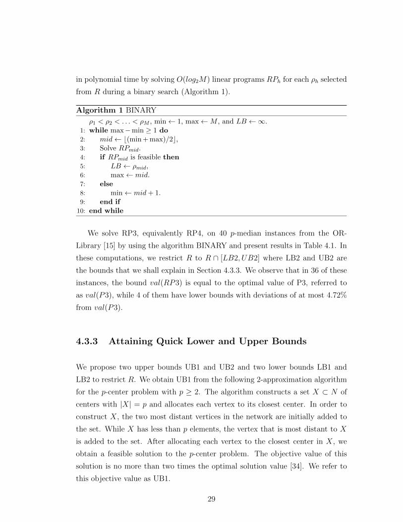
in polynomial time by solving O(log2M) linear programs RPh for each ρh selected

from R during a binary search (Algorithm 1).

Algorithm 1 BINARY

ρ1 < ρ2 < . . . < ρM , min← 1, max←M , and LB ←∞.1: while max−min ≥ 1 do2: mid← b(min + max)/2c,3: Solve RPmid.4: if RPmid is feasible then5: LB ← ρmid,6: max← mid.7: else8: min← mid+ 1.9: end if

10: end while

We solve RP3, equivalently RP4, on 40 p-median instances from the OR-

Library [15] by using the algorithm BINARY and present results in Table 4.1. In

these computations, we restrict R to R ∩ [LB2, UB2] where LB2 and UB2 are

the bounds that we shall explain in Section 4.3.3. We observe that in 36 of these

instances, the bound val(RP3) is equal to the optimal value of P3, referred to

as val(P3), while 4 of them have lower bounds with deviations of at most 4.72%

from val(P3).

4.3.3 Attaining Quick Lower and Upper Bounds

We propose two upper bounds UB1 and UB2 and two lower bounds LB1 and

LB2 to restrict R. We obtain UB1 from the following 2-approximation algorithm

for the p-center problem with p ≥ 2. The algorithm constructs a set X ⊂ N of

centers with |X| = p and allocates each vertex to its closest center. In order to

construct X, the two most distant vertices in the network are initially added to

the set. While X has less than p elements, the vertex that is most distant to X

is added to the set. After allocating each vertex to the closest center in X, we

obtain a feasible solution to the p-center problem. The objective value of this

solution is no more than two times the optimal solution value [34]. We refer to

this objective value as UB1.

29

Table 4.1: The lower bounds val(RP3) and solution times of RP3 for OR-Libraryinstances

Instance n p val(P3) val(RP3) Gap (%) Time (sec)pmed1 100 5 127 121 4.72 0.19pmed2 100 10 98 98 0 0.04pmed3 100 10 93 93 0 0.03pmed4 100 20 74 74 0 0.02pmed5 100 33 48 48 0 0.02pmed6 200 5 84 83 1.19 0.07pmed7 200 10 64 64 0 0.09pmed8 200 20 55 55 0 0.05pmed9 200 40 37 37 0 0.04pmed10 200 67 20 20 0 0.03pmed11 300 5 59 59 0 0.10pmed12 300 10 51 51 0 0.12pmed13 300 30 36 36 0 0.06pmed14 300 60 26 26 0 0.08pmed15 300 100 18 18 0 0.02pmed16 400 5 47 47 0 0.14pmed17 400 10 39 39 0 0.17pmed18 400 40 28 28 0 0.10pmed19 400 80 18 18 0 0.06pmed20 400 133 13 13 0 0.04pmed21 500 5 40 40 0 0.20pmed22 500 10 38 38 0 0.33pmed23 500 50 22 22 0 0.16pmed24 500 100 15 15 0 0.09pmed25 500 167 11 11 0 0.05pmed26 600 5 38 37 2.63 0.38pmed27 600 10 32 32 0 0.34pmed28 600 60 18 18 0 0.2pmed29 600 120 13 13 0 0.14pmed30 600 200 9 9 0 0.09pmed31 700 5 30 30 0 0.31pmed32 700 10 29 28 3.45 0.50pmed33 700 70 15 15 0 0.28pmed34 700 140 11 11 0 0.13pmed35 800 5 30 30 0 0.46pmed36 800 10 27 27 0 0.57pmed37 800 80 15 15 0 0.44pmed38 900 5 29 29 0 0.68pmed39 900 10 23 23 0 0.93pmed40 900 90 13 13 0 0.38Average: 0.20

30

We obtain UB2 by making an improvement on the above algorithm. Let

x1, . . . , xp be the set of centers selected. We divide the network into p clusters

I1, . . . , Ip where Ij is the set of vertices allocated to center xi (break ties arbi-

trarily). Let Ti = maxd(xi, j) : j ∈ Ii for i ∈ 1, . . . , p. Then, the objective

value of the current solution is Tmax = maxi=1,...,p

Ti. In order to improve the ob-

tained solution, we solve a 1-center problem in each of these clusters by using the

method proposed in [4]. We start with cluster Ii, where Ti = Tmax and obtain

a new radius value T i ≤ Ti. If T i = Ti, we stop the algorithm. If T i < Ti, we

set Tmax = T i. Then we solve a 1-center problem for each remaining cluster Ik if

Tk > Tmax and set Tmax = T k if = T k > Tmax. Obviously, we will have a solution

which is no worse than the initial one after this improvement procedure. Thus,

we can conclude that our algorithm is a 2-approximation algorithm. We refer to

this solution value as UB2.

LB1 is obtained as follows: Suppose we sort positive distance values in non-

decreasing order as β1 ≤ β2 ≤ . . . ≤ βn×(n−1) (ties are allowed in the sequence)

and let X = x1, x2, . . . , xp ⊂ N be an optimal p-center. Then the remaining

n − p vertices need to be served by these centers. Even if we assume that each

vertex is served by its closest center, the maximum of the closest distance values

cannot be smaller than βn−p since val(P3) = maxi∈N\X

minxj∈X

dixj ≥ βn−p. We refer to

this lower bound as LB1.

LB2 is obtained from UB1: Since UB1 is less than or equal to two times

the optimal value, (UB1)/2 provides a lower bound on the optimal value. We

improve this lower bound one more step and select the smallest distance value

in R, which is greater than or equal to (UB1)/2, as a lower bound (LB2) for the

p-center problem.

We compute the LB1, LB2, UB1 and UB2 values for the 40 p-median in-

stances and give the results obtained in Table 4.2 and Table 4.3. The gap values

reported in Table 4.2 and Table 4.3 are equal to (Value−val(P3))/val(P3) and

(val(P3)−Value)/val(P3), respectively, where ‘Value’ represents the correspond-

ing bound value. When we compare the values of UB1 and UB2, we see that

in 23 of these instances, UB2 value is smaller than UB1 value. This means that

31

the improvement stage is helpful in obtaining a solution with better objective

in these instances. In the other instances, the improvement stage is not able to

find a solution with a smaller objective value; thus, UB2 value equals UB1 value.

When the values of LB1 and LB2 are compared, we observe that LB2 value is

larger than LB1 value for each instance. Each of these lower and upper bounds is

obtained in at most 0.06 seconds, which is much faster than the calculation times

of any relaxation bound discussed. When we compare LB2 with val(LP4) and

val(RP3), we see that LB2 and val(LP4) values are quite close to each other and

val(RP3) is greater than both of them for each instance. Since we can obtain

LB2 values very quickly, we decided to use LB2 and UB2 values to restrict the

set R when we make experiments with the proposed model P3 and double bound

algorithms. For any problem tested in this chapter, LB2 and UB2 values can be

obtained in less than 1 second. Therefore, we do not add the calculation times

of these bounds to the solution times reported in the tables of the remaining

sections of this chapter.

4.4 Double Bound Algorithms

Let S be any nonempty subset of T = 1, . . . ,M and define P (S) to be the

problem which is exactly the same as P3 except that all variables zk, k ∈ T \ S,

are dropped from P3. This amounts to replacing the index set T in (4.12)-(4.15)

with the index set S. Let val(P (S)) be the optimal value of P (S) with P (S) =∞if P (S) is infeasible.

Proposition 2. Suppose |S| > 2. Let a and b be the smallest and largest indices

in S, respectively.

(a) If val(P (S)) = ρa, then r∗V ∈ ρ1, . . . , ρa.

(b) If val(P (S)) = ρk for some k with a < k ≤ b, then r∗V ∈ ρk′+1, . . . , ρkwhere k′ is the largest index in S which is smaller than k.

(c) If val(P (S)) =∞, then r∗V ∈ ρb+1, . . . , ρM.

32

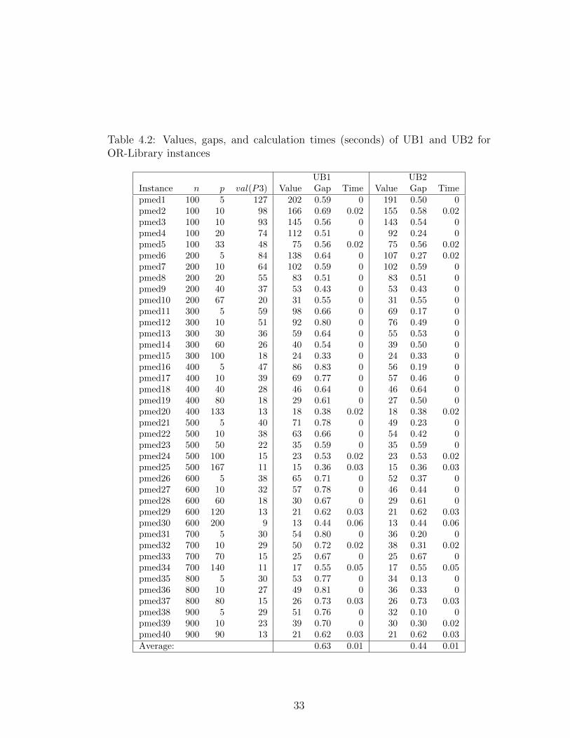
Table 4.2: Values, gaps, and calculation times (seconds) of UB1 and UB2 forOR-Library instances

UB1 UB2Instance n p val(P3) Value Gap Time Value Gap Timepmed1 100 5 127 202 0.59 0 191 0.50 0pmed2 100 10 98 166 0.69 0.02 155 0.58 0.02pmed3 100 10 93 145 0.56 0 143 0.54 0pmed4 100 20 74 112 0.51 0 92 0.24 0pmed5 100 33 48 75 0.56 0.02 75 0.56 0.02pmed6 200 5 84 138 0.64 0 107 0.27 0.02pmed7 200 10 64 102 0.59 0 102 0.59 0pmed8 200 20 55 83 0.51 0 83 0.51 0pmed9 200 40 37 53 0.43 0 53 0.43 0pmed10 200 67 20 31 0.55 0 31 0.55 0pmed11 300 5 59 98 0.66 0 69 0.17 0pmed12 300 10 51 92 0.80 0 76 0.49 0pmed13 300 30 36 59 0.64 0 55 0.53 0pmed14 300 60 26 40 0.54 0 39 0.50 0pmed15 300 100 18 24 0.33 0 24 0.33 0pmed16 400 5 47 86 0.83 0 56 0.19 0pmed17 400 10 39 69 0.77 0 57 0.46 0pmed18 400 40 28 46 0.64 0 46 0.64 0pmed19 400 80 18 29 0.61 0 27 0.50 0pmed20 400 133 13 18 0.38 0.02 18 0.38 0.02pmed21 500 5 40 71 0.78 0 49 0.23 0pmed22 500 10 38 63 0.66 0 54 0.42 0pmed23 500 50 22 35 0.59 0 35 0.59 0pmed24 500 100 15 23 0.53 0.02 23 0.53 0.02pmed25 500 167 11 15 0.36 0.03 15 0.36 0.03pmed26 600 5 38 65 0.71 0 52 0.37 0pmed27 600 10 32 57 0.78 0 46 0.44 0pmed28 600 60 18 30 0.67 0 29 0.61 0pmed29 600 120 13 21 0.62 0.03 21 0.62 0.03pmed30 600 200 9 13 0.44 0.06 13 0.44 0.06pmed31 700 5 30 54 0.80 0 36 0.20 0pmed32 700 10 29 50 0.72 0.02 38 0.31 0.02pmed33 700 70 15 25 0.67 0 25 0.67 0pmed34 700 140 11 17 0.55 0.05 17 0.55 0.05pmed35 800 5 30 53 0.77 0 34 0.13 0pmed36 800 10 27 49 0.81 0 36 0.33 0pmed37 800 80 15 26 0.73 0.03 26 0.73 0.03pmed38 900 5 29 51 0.76 0 32 0.10 0pmed39 900 10 23 39 0.70 0 30 0.30 0.02pmed40 900 90 13 21 0.62 0.03 21 0.62 0.03Average: 0.63 0.01 0.44 0.01

33

Table 4.3: Values, gaps, and calculation times (seconds) of LB1 and LB2 forOR-Library instances

LB1 LB2Instance n p val(P3) Value Gap Time Value Gap Timepmed1 100 5 127 59 0.54 0 101 0.20 0pmed2 100 10 98 56 0.43 0 83 0.15 0.02pmed3 100 10 93 55 0.41 0 73 0.22 0pmed4 100 20 74 41 0.45 0 56 0.24 0pmed5 100 33 48 23 0.52 0 38 0.21 0.02pmed6 200 5 84 38 0.55 0 69 0.18 0pmed7 200 10 64 34 0.47 0 51 0.20 0pmed8 200 20 55 30 0.45 0 42 0.24 0pmed9 200 40 37 22 0.41 0 27 0.27 0pmed10 200 67 20 11 0.45 0 16 0.20 0pmed11 300 5 59 34 0.42 0 49 0.17 0pmed12 300 10 51 30 0.41 0 46 0.10 0pmed13 300 30 36 20 0.44 0.02 30 0.17 0pmed14 300 60 26 14 0.46 0 20 0.23 0pmed15 300 100 18 10 0.44 0 12 0.33 0pmed16 400 5 47 26 0.45 0 43 0.09 0pmed17 400 10 39 21 0.46 0 35 0.10 0pmed18 400 40 28 16 0.43 0 23 0.18 0pmed19 400 80 18 10 0.44 0 15 0.17 0pmed20 400 133 13 7 0.46 0 9 0.31 0.02pmed21 500 5 40 23 0.43 0.02 36 0.10 0pmed22 500 10 38 21 0.45 0 32 0.16 0pmed23 500 50 22 13 0.41 0 18 0.18 0pmed24 500 100 15 9 0.40 0 12 0.20 0.02pmed25 500 167 11 6 0.45 0 8 0.27 0.03pmed26 600 5 38 21 0.45 0 33 0.13 0pmed27 600 10 32 18 0.44 0 29 0.09 0pmed28 600 60 18 10 0.44 0.02 15 0.17 0pmed29 600 120 13 7 0.46 0 11 0.15 0.03pmed30 600 200 9 5 0.44 0 7 0.22 0.06pmed31 700 5 30 16 0.47 0 27 0.10 0pmed32 700 10 29 16 0.45 0.02 25 0.14 0.02pmed33 700 70 15 9 0.40 0.02 13 0.13 0pmed34 700 140 11 6 0.45 0.02 9 0.18 0.05pmed35 800 5 30 16 0.47 0.02 27 0.10 0pmed36 800 10 27 16 0.41 0 25 0.07 0pmed37 800 80 15 8 0.47 0.02 13 0.13 0.03pmed38 900 5 29 15 0.48 0.02 26 0.10 0pmed39 900 10 23 13 0.43 0.02 20 0.13 0pmed40 900 90 13 7 0.46 0.02 11 0.15 0.03Average: 0.45 0.01 0.17 0.01

34

Proof. Since S is a subset of T , P (S) is a restriction of P3. Hence, val(P3) ≤val(P (S)). We have r∗V = val(P3) from Proposition 1 implying that r∗V ≤ ρa if

(a) holds. This proves (a). To prove (b), observe that val(P (S)) = ρk and k > a

imply that Pk is feasible while Pk′ is infeasible. Accordingly, ρk′ < r∗V ≤ ρk which

gives r∗V ∈ ρk′+1, . . . , ρk. To prove (c), observe that val(P (S)) = ∞ implies

that Pb is infeasible. Hence, r∗V ∈ ρb+1, . . . , ρM.

This proposition allows devising a search strategy based on restrictions of P3

or P4. The main idea is the following: Select a nonempty subset S of T and solve

P (S). Depending on which of (a), (b) or (c) occurs in Proposition 2, delete from

T the set of indices k such that ρk cannot equal r∗V . Select a new subset S of

T after deletions and repeat the procedure. Termination occurs when T reduces

to a singleton. The computational success of such a procedure depends on how

efficiently we solve each subproblem, P (S), as well as how many times we have

to solve a new problem. We give below a specialized way of doing this with sets

S containing two elements. The method is called the double bound method. Six

variations are discussed.

The double bound algorithm solves P (S) for S = a, b where a, b ∈ T with

a < b. Let T1 = 1, . . . , a, T2 = a + 1, . . . , b and T3 = b + 1, . . . ,M. We

may solve P (S) directly or solve Pa and Pb separately. The former problem

involves m + 2 binary variables while each of the latter problems involves m

binary variables. After solving P (S), we know which one of the subsets T1, T2

and T3 contains the optimal value of the p-center problem. Since we do not need

to consider two of these subsets anymore, we repeat the procedure with the subset

that contains the optimal value until we have a single element subset on hand. We

propose three ways to choose a and b in Table 4.4. For each choice, we give two

types of algorithms, one type solving P (S) directly (referred to as DB algorithms)

and the other solving Pa and Pb separately to obtain a solution to P (S) (referred

to as DBR algorithms). The initial steps and the terminations of the algorithms

are the same. The algorithms work with the ordered list R = ρ1, . . . , ρM. We

provide a general scheme of the double bound algorithm in Figure 1. Note that

the DBR algorithms are identical for solving P3 and P4.

35

Table 4.4: Selection of radius values for the double bound algorithm

(a, b) Together Separatelya = b(max + min)/2c

DB1 DBR1b = maxa = b(max + min)/2c

DB2 DBR2b = max−1a = min +b(max−min)/3c

DB3 DBR3b = min +2b(max−min)/3c

Figure 4.1: General scheme of the double bound algorithm

36

In the worst case, DB1, DBR1, DB2 and DBR2 algorithms terminate in

O(log2M) iterations and DB3, DBR3 algorithms terminate in O(log3M) itera-

tions. Suppose we are at the beginning of some iteration of our DB2 algorithm and

we have an a value and a max value. Then we solve P (S) for S = a,max−1.If r∗V equals ρmax of this iteration, then P (S) becomes infeasible and we terminate

the algorithm at the end of this iteration. This quick termination is also available

in DBR2 algorithm. In DB1 algorithm, we solve P (S) for S = a,max. If r∗V

equals ρmax of the current iteration, we cannot know this until we solve P (S) for

S = max−1,max and this takes O(log2(max−a)) iterations. This is also valid

for DBR1 algorithm. In the same case, DB3 and DBR3 algorithms terminate

after O(log3(max−b)) iterations.

4.5 Computational Experiments

In the computational experiments of this chapter, we follow the general trend

in the literature and take J = N . The input data used for the computations

consists of the p-median data from OR-Library [15] for 40 instances with n varying

between 100 and 900 and p varying between 5 and (n/3) and some instances from

TSPLIB [16]. The original data in OR-Library [15] consists of a listing of edges

and their lengths. By using the all-pairs shortest path algorithm due to Floyd

[62] on this data, we obtain the distance matrix D. In TSPLIB [16] instances,

the coordinates of the vertices are provided. We calculate the Euclidean distance

for each vertex pair and round it to the nearest integer. Note that rounding

might destroy the triangular inequality, but we are safe since we do not require

this property in our methods. We solve problems from u1817 with n = 1817,

from d15112 with n = 2500 and from pcb3038 with n = 3038. During our

computations we use JCreator LE 4.50 [63] and IBM ILOG CPLEX 12.4 [64] with

concert technology. In all mathematical models that we solve in this chapter, we

set MIPEmphasis option of CPLEX to 1. For the algorithms DBR1, DBR2 and

DBR3, we additionally set IntSolLim to 1.

In all tables of this section, the first three columns give the characteristics

37

of the instances and the column labeled “Opt” gives the optimal p-radii. The

reported solution times in tables are in seconds. We provide the results of the ex-

periments on the unweighted problems in Section 4.5.1 and the weighted problems

in Section 4.5.2.

4.5.1 Unweighted Problems

While P1 is a more compact formulation of the p-center problem than P2, P3 and

P4, the computational performances of P2, P3 and P4 are far better than that of

P1 when all four formulations are directly solved by a commercial solver. Table 4.5

gives a comparison of solution times and optimal or best-found objective values

for P1, P2, P3 and P4 for the vertex restricted case using 40 p-median instances

taken from the OR-Library [15]. The possible values of r∗V in R that are needed

in P2, P3 and P4 are restricted to a subset R′ ≡ R ∩ [LB2, UB2]. In this table,

columns 5, 6, 7 and 8 give the solution times in seconds taken by the solver for

the IP models P4, P3, P2 and P1, respectively. While solving the four IP models,

we put a time restriction of three hours. P2, P3 and P4 can solve each problem

optimally within the three hour limit while P1 cannot solve 17 of these problems

optimally. Of the 17 unsolved instances, 5 of them are instances for which no

feasible integer solution can be found by P1 within the three hour limit. These are

indicated by NFS (No Feasible Solution) in the middle column under P1 in the

table. For the 12 instances that are solved sub-optimally by P1, the last column

under P1 gives the percent gap reported by CPLEX. When we compare P2, P3

and P4 with each other, we see that the largest time required is 772.68 seconds

for P4 (instance pmed39) while it is 1232.92 seconds for P3 (instance pmed39)

and 1428.94 seconds for P2 (instance pmed8). The average time required to solve

40 instances with P4 is 82.25 seconds while it is 99.80 seconds for P3 and 155.25

seconds for P2. The differences in computational times are more significant in

some instances. For example, P3 solves pmed8 in 10.31 seconds and P4 solves

the same instance in 12.74 seconds while P2 solves it in 1428.94 seconds, which is

more than 138 times that of P3 and 112 times that of P4. Among 40 instances,

for 7 of them P2 achieves the smallest solving time while P3 is the successor for

38

22 of them and P4 is the successor for 11 of them. We may conclude from these

observations that the proposed model P3 and its tightened version P4 perform

noticeably better than P2 on the 40 p-median instances taken from OR-Library

[15] and that P2, P3 and P4 perform significantly better than P1. While direct

solution times are reasonable for P2, P3 and P4, the double bound algorithms

lead to much shorter solution times than direct solution times available in this

table.

We compare the performance of our algorithms on 40 p-median instances in

Table 4.6. The first observation from this table is that the double bound al-

gorithms perform much better than solving P3 or P4 directly (See Table 4.5.).

The solution times of the double bound algorithms are much better for all in-

stances than direct solution times. When we compare the double bound algo-

rithms among themselves, we see that they all show similar performance in terms

of time requirements for the instances with n =100 or 200. As n goes up from

200 to 900, the DBR algorithms take considerably less time to terminate than

DB algorithms. This is also reflected in the average time requirements of the

algorithms. Each instance in this table is solved in less than 3 seconds by DBR

algorithms and in less than 27 seconds by DB algorithms.

To see the computational performance of the proposed algorithms on larger

problems, we conducted experiments on u1817 data from TSPLIB [16]. This

problem has 1817 nodes and is solved with 18 different p values. We observed

in the tests that the DB algorithms require significantly more time to arrive at

optimal solutions than DBR algorithms. For this reason, we give the results only

for the DBR algorithms.

Table 4.7 gives the solution times for the DBR algorithms on 20 instances

from TSP-Library with n=1817. We again restrict R by using LB2 and UB2

values in these experiments and these values are given in the fifth and sixth

columns, respectively. The solution times of the algorithms are given in the last

three columns. For the highlighted instances in this table, the optimal values are

provided for the first time in the literature. Elloumi et al. [1] conduct experiments

on the first 15 instances of this table, but they are not able to solve optimally

39

Table 4.5: Solution times (seconds) of IP models

P4 P3 P2 P1Instance n p Opt Time Time Time Time Obj Gap%pmed1 100 5 127 11.33 4.38 52.78 188.81 127pmed2 100 10 98 7.0 2.00 12.94 73.34 98pmed3 100 10 93 5.26 1.90 7.72 37.89 93pmed4 100 20 74 1.30 0.21 8.35 0.90 74pmed5 100 33 48 1.08 0.26 1.45 0.39 48pmed6 200 5 84 11.50 15.81 33.50 2797.12 84pmed7 200 10 64 26.89 16.67 96.79 4476.78 64pmed8 200 20 55 12.74 10.31 1428.94 776.21 55pmed9 200 40 37 4.71 0.68 3.57 6.40 37pmed10 200 67 20 0.62 0.13 0.34 1.40 20pmed11 300 5 59 9.09 15.08 14.01 537.31 59pmed12 300 10 51 34.74 38.42 28.93 7115.81 51pmed13 300 30 36 16.05 19.83 42.15 3188.15 36pmed14 300 60 26 5.60 2.19 4.92 281.05 26pmed15 300 100 18 1.33 0.29 0.81 3.82 18pmed16 400 5 47 5.76 4.18 33.91 10800.00 47 6.78pmed17 400 10 39 45.21 50.32 38.33 10800.00 41 14.63pmed18 400 40 28 71.64 48.98 55.39 10539.49 28pmed19 400 80 18 4.91 2.24 5.43 33.34 18pmed20 400 133 13 1.33 0.28 0.75 3.79 13pmed21 500 5 40 12.36 17.95 35.65 10800.00 43 16.28pmed22 500 10 38 239.84 373.73 1223.58 10800.00 41 18.37pmed23 500 50 22 185.59 54.86 129.87 10800.00 24 16.67pmed24 500 100 15 10.33 3.46 4.78 439.70 15pmed25 500 167 11 1.61 0.26 0.73 17.13 11pmed26 600 5 38 32.64 72.78 57.96 10800.00 39 10.26pmed27 600 10 32 95.41 295.62 201.31 10800.00 40 25.00pmed28 600 60 18 180.21 75.00 46.47 10800.00 20 19.72pmed29 600 120 13 19.19 7.24 12.28 1976.99 13pmed30 600 200 9 1.25 0.31 0.70 5.29 9pmed31 700 5 30 19.75 15.70 34.13 10800.00 NFSpmed32 700 10 29 351.59 407.49 949.57 10800.00 38 32.89pmed33 700 70 15 177.61 180.43 213.66 10800.00 17 17.46pmed34 700 140 11 22.98 6.91 7.59 3159.30 11pmed35 800 5 30 18.38 14.53 14.25 10800.00 NFSpmed36 800 10 27 358.30 414.04 227.85 10800.00 NFSpmed37 800 80 15 186.11 268.12 154.61 10800.00 25 47.64pmed38 900 5 29 17.64 20.63 19.53 10800.00 NFSpmed39 900 10 23 772.68 1232.82 837.51 10800.00 NFSpmed40 900 90 13 308.41 295.98 167.11 10800.00 20 40.00Average: 82.25 99.80 155.25 5481.51

40

Table 4.6: Times (seconds) required to solve P3 with DB and DBR algorithmson 40 p-median instances

Instance n p DB1 DB2 DB3 DBR1 DBR2 DBR3pmed1 100 5 0.41 0.58 0.55 0.46 0.54 0.54pmed2 100 10 0.17 0.15 0.31 0.19 0.23 0.23pmed3 100 10 0.19 0.13 0.18 0.20 0.21 0.12pmed4 100 20 0.19 0.18 0.41 0.11 0.13 0.21pmed5 100 33 0.13 0.18 0.11 0.10 0.12 0.09pmed6 200 5 0.68 0.80 0.60 0.29 0.32 0.23pmed7 200 10 0.38 0.32 0.48 0.18 0.18 0.20pmed8 200 20 0.26 0.37 0.49 0.14 0.19 0.17pmed9 200 40 0.16 0.27 0.23 0.12 0.20 0.20pmed10 200 67 0.10 0.06 0.27 0.09 0.10 0.06pmed11 300 5 0.63 0.65 0.50 0.43 0.54 0.31pmed12 300 10 0.79 0.71 0.96 0.28 0.32 0.30pmed13 300 30 0.44 0.45 0.66 0.26 0.30 0.27pmed14 300 60 0.30 0.30 0.37 0.12 0.15 0.13pmed15 300 100 0.11 0.11 0.30 0.05 0.07 0.09pmed16 400 5 1.12 0.91 1.00 0.44 0.55 0.50pmed17 400 10 1.43 0.78 1.12 0.43 0.33 0.38pmed18 400 40 0.93 0.82 0.87 0.15 0.17 0.14pmed19 400 80 0.39 0.38 0.37 0.11 0.11 0.09pmed20 400 133 0.17 0.13 0.13 0.05 0.05 0.06pmed21 500 5 1.99 1.66 1.49 0.81 0.95 0.92pmed22 500 10 3.07 3.26 3.43 1.06 1.08 0.99pmed23 500 50 1.42 1.41 1.67 0.22 0.31 0.29pmed24 500 100 0.58 0.42 0.24 0.14 0.14 0.09pmed25 500 167 0.26 0.18 0.17 0.07 0.07 0.07pmed26 600 5 5.68 6.25 4.31 1.62 1.61 1.15pmed27 600 10 4.23 3.56 3.29 0.98 0.94 0.89pmed28 600 60 2.34 2.05 1.73 0.27 0.29 0.24pmed29 600 120 0.76 0.87 0.45 0.14 0.18 0.14pmed30 600 200 0.32 0.24 0.28 0.09 0.08 0.13pmed31 700 5 4.20 5.22 2.51 1.32 2.03 1.22pmed32 700 10 6.62 5.52 7.39 1.91 2.35 2.12pmed33 700 70 3.55 2.69 1.60 0.37 0.33 0.28pmed34 700 140 0.90 0.50 0.70 0.16 0.15 0.22pmed35 800 5 6.88 4.42 5.29 1.72 1.69 1.72pmed36 800 10 12.86 7.30 9.82 2.14 2.71 1.96pmed37 800 80 6.38 4.02 3.01 0.46 0.40 0.31pmed38 900 5 11.44 6.63 6.67 2.53 2.55 2.61pmed39 900 10 12.00 26.50 23.56 2.69 2.59 1.57pmed40 900 90 7.59 6.29 3.37 0.47 0.61 0.44Average: 2.55 2.43 2.27 0.58 0.65 0.54

41

Table 4.7: Results of DBR algorithms for solving P3 or P4 for TSPLIB instanceswith n=1817

Instance n p Opt LB2 UB2 DBR1 DBR2 DBR3

u1817 1817 10 458 301 585 27.92 22.11 25.45u1817 1817 20 309 191 357 305.45 278.49 452.52u1817 1817 30 241 166 331 274.13 344.59 147.97u1817 1817 40 209 155 307 789.89 1221.86 896.55u1817 1817 50 185 127 229 332.89 330.09 643.78u1817 1817 60 163 105 209 16.38 17.52 13.14u1817 1817 70 148 99 194 6.02 6.04 9.93u1817 1817 80 137 93 185 26.79 35.12 24.95u1817 1817 90 129 90 180 8619.10 7519.04 9545.52u1817 1817 100 127 86 170 7.26 10.22 12.6u1817 1817 110 110 81 161 4.87 5.32 5.33u1817 1817 120 107 74 148 3.16 3.99 2.99u1817 1817 130 105 71 137 337.57 335.03 373.23u1817 1817 140 102 68 129 7.73 4.62 9.11u1817 1817 150 92 64 127 6.52 6.61 6.73u1817 1817 200 80 56 105 2.1 2.56 2.37u1817 1817 250 76 46 92 1.26 2.17 1.42u1817 1817 300 63 46 80 0.87 2.01 0.89

Average: 598.33 563.74 676.36

the highlighted instances. The algorithms spend an excessive amount of time for

solving the problem with p=90. DBR2 shows the best performance and DBR3

shows the worst performance for this instance. Another instance that results

in a considerable difference between the performances of the algorithms is the

problem with p=40. DBR1 performs the best and DBR2 performs the worst for

this instance. For the other instances, the time requirements of the algorithms

are very close to each other. On the average, DBR2 spends the least amount of

time and DBR3 spends the largest amount of time.

We select DBR2 as the winner of the six DB and DBR algorithms and solve

larger problems with n ∈ 1817, 2500, 3008 from the TSPLIB [16] by using

the lower bound val(RP3). We compute this bound by solving O(log2M) LP

problems RPh using Algorithm 1 with R restricted to R ∩ [LB2, UB2]. The

bounds val(RP3) are generally computed in a matter of seconds. The minimum,

average and maximum computing times for 33 instances are 0.59, 33.16 and 166

42

seconds, respectively. We also note that the lower bound val(RP3) is equal

to the optimal value of P3 for 8 instances of the TSPLIB [16] problems with

n ∈ 1817, 2500, 3008 while the gap between them is at most 0.053 for the

remaining instances.

Table 4.8 gives the relevant statistics for solving P3 via the algorithm DBR2

by restricting R to R ∩ [val(RP3), UB2]. For the 33 instances reported in Table

4.8, a time limit of three hours is imposed for each problem Ph ∈ Pmid, Pmax−1attempted in main steps of the algorithm DBR2. At the end of three hours,

either a solution is found for Ph or the infeasibility of Ph is detected or the fea-

sibility/infeasibility status of Ph remains unknown. If the status of Ph remains

unknown, we solve the problems Ph+1, Ph+2, etc. with successively increasing

radius values until a feasible solution is found within three hours for some prob-

lem Ph+k. This gives us an upper bound ρh+k on r∗V that is the best (smallest)

bound that can be confirmed within the time limit. Similarly, we solve problems

Ph−1, Ph−2, etc. with successively decreasing radius values until we detect infeasi-

bility of some Ph−k′ within the time limit. This gives us a lower bound ρh−k′+1 on

r∗V that is the largest possible that can be confirmed within the time limit. Thus,

r∗V ∈ ρh−k′+1, . . . , ρh+k. The values ρh−k′+1 and ρh+k are reported as the “Best

LB” and “Best UB” in the table in columns 5 and 6, respectively. Column 7

gives the gap between the “Best UB” and “Best LB” values while column 4 gives

the optimal values for P3. If the optimal solution is found for a problem within

three hours, the values in columns 4, 5 and 6 are equal. For such problems, the

gaps in column 7 are zero. Column 8 gives the solution times obtained by the

algorithm DBR2. For all of the instances with n = 1817, we obtain the optimal

solution. The most time consuming instance among them is the one with p = 40.

This instance is solved in 1225 seconds. For the problems with n = 2500, we

obtain the optimal solution for all instances except the one with p = 100. The

gap between the best upper bound and the best lower bound we obtain for this

instance is 0.008. The optimal solutions for the six instances with n = 3038 are

obtained. For the remaining instances the gap between the best bounds is at

most 0.027. For any of the reported network sizes, all instances with p = 5 and

10 are solved in less than three minutes and all instances with p = 400 and 500

43

are solved in less than 12 seconds.

Before solving the individual problem Pk for some k ∈ T in the main steps of

DBR2 algorithm, it is possible to eliminate some of the variables and constraints

by applying the reduction rules which are well known for the set covering problem

[65]. These rules not only detect any infeasibility immediately, but also reveal

the optimal value of some decision variables and the dominance relation between

the constraints. We utilized these reduction rules in our algorithm to solve the

instances that require large amount of time (more than one hour) and provided

the results in Table 4.9. One of the instances in this table is taken from Table 4.7

and the others are taken from Table 4.8. Table 4.9 consists of the same columns as

in Table 4.8 except that it has an additional column “PP Time” which represents

the total time consumed for the reduction procedure. Among the 13 instances

in this table, for 11 of them reduction makes an improvement in terms of either

the best LB, the best UB or in the total time and those improved parameters

are depicted in bold. We observe that the maximum gap between the best LB

and the best UB decreases from 0.027 to 0.022 and we are able to obtain the

optimal solution for the instance with n = 3038 and p = 30. For some instances

the total time consumption decreases significantly. For instance, the total time

consumed decreases around 85% for the first instance and 84% for the second

instance in Table 4.9. The average decrease in total time is 61% for the instances

with decrease in time and 38% for all instances. When we subtract the reduction

time from the total time, we can observe how much reduction helps CPLEX to

solve the problems. The average of this improvement is 60% for the improved

instances and 49% for all instances. These experiments reveal that the reduction

rules are quite helpful in solving both individual problems Pk for k ∈ T and P3

via DBR2 algorithm.

4.5.2 Weighted Problems

In this section, we solve weighted problems by using the DBR2 algorithm. We

generate the weights of the nodes uniformly between 1 and 10. Table 4.10 presents

the results we obtain from 40 OR-Library [15] instances. The average solution

44

Table 4.8: Results of algorithm DBR2 for solving problem P3 or P4 for TSPLIBinstances with n ∈ 1817, 2500, 3038

Instance n p val(P3) Best LB BestUB Gap Time (sec)

u1817 1817 5 715 715 715 0 14.10u1817 1817 10 458 458 458 0 20.31u1817 1817 20 309 309 309 0 257.68u1817 1817 30 241 241 241 0 204.77u1817 1817 40 209 209 209 0 1225.00u1817 1817 50 185 185 185 0 314.46u1817 1817 100 127 127 127 0 7.43u1817 1817 200 80 80 80 0 2.57u1817 1817 300 63 63 63 0 1.19u1817 1817 400 51 51 51 0 0.84u1817 1817 500 51 51 51 0 0.23

d15112 2500 5 5856 5856 5856 0 95.91d15112 2500 10 3705 3705 3705 0 84.85d15112 2500 20 2573 2573 2573 0 288.12d15112 2500 30 2029 2029 2029 0 5293.59d15112 2500 40 1723 1723 1723 0 21899.83d15112 2500 50 1524 1524 1524 0 5782.76d15112 2500 100 1049 1057 0.008 94245.98d15112 2500 200 723 723 723 0 28371.08d15112 2500 300 571 571 571 0 38.39d15112 2500 400 481 481 481 0 4.99d15112 2500 500 424 424 424 0 4.84

pcb3038 3038 5 1064 1064 1064 0 116.74pcb3038 3038 10 729 729 729 0 176.28pcb3038 3038 20 493 493 493 0 22740.76pcb3038 3038 30 391 397 0.015 76923.67pcb3038 3038 40 331 337 0.018 72364.56pcb3038 3038 50 292 300 0.027 91029.77pcb3038 3038 100 207 209 0.010 27292.39pcb3038 3038 200 138 141 0.022 33929.91pcb3038 3038 300 115 115 115 0 6185.96pcb3038 3038 400 97 97 97 0 11.48pcb3038 3038 500 85 85 85 0 5.23

45

Table 4.9: Results with utilization of the reduction rules

PP Time Total TimeInstance n p val(P3) Best LB Best UB Gap (sec) (sec)u1817 1817 90 129 129 129 0 578.59 1225.76d15112 2500 30 2029 2029 2029 0 108.25 865.63d15112 2500 40 1723 1723 1723 0 132.37 6831.56d15112 2500 50 1524 1524 1524 0 158.75 1645.55d15112 2500 100 1050 1059 0.009 416.46 104013.04d15112 2500 200 723 723 723 0 482.84 5293.26pcb3038 3038 20 493 493 493 0 3102.33 6800.68pcb3038 3038 30 393 393 393 0 4063.66 52285.79pcb3038 3038 40 332 337 0.015 4920.76 75702.72pcb3038 3038 50 293 299 0.020 6199.33 80313.04pcb3038 3038 100 207 208 0.005 4483.28 15717.50pcb3038 3038 200 138 141 0.022 6060.09 42621.69pcb3038 3038 300 115 115 115 0 3701.42 6569.00

time in this table is slightly larger than the average solution time obtained from

solving the unweighted problems in Table 4.6. However, when we look at Tables

4.11 and 4.12, we can observe that the weighted problems are solved faster when

compared to the solution times of the unweighted problems in Tables 4.7 and 4.8.

This is an expected result since breaking symmetry typically eases a problem.

4.6 Conclusion

In this chapter, we proposed a new IP formulation for the p-center problem. By

tightening one set of constraints in our model, we obtained a modified model

with much better LP bounds. When compared with the two models from the

literature, both of our models performed better in terms of the time requirement.

The LP bounds of our tightened model are equivalent to the LP bounds of the

model proposed by [1] and they are the strongest LP bounds among those of the

four models. We obtained a stronger lower bound from our models by relaxing

one set of binary variables and this lower bound is equivalent to the best known

lower bound in the literature. We also provided a polynomial time algorithm

to obtain this lower bound. In addition to the relaxation bounds, we proposed

new lower and upper bounds which can be computed very quickly and we used

46

Table 4.10: Results for solving P3 or P4 with DBR2 algorithm on weighted OR-Library instances

Instance n p Opt Time (sec)pmed1 100 5 2292 0.44pmed2 100 10 1605 0.60pmed3 100 10 1539 0.28pmed4 100 20 1176 0.40pmed5 100 33 664 0.05pmed6 200 5 1410 0.52pmed7 200 10 1156 0.44pmed8 200 20 882 0.35pmed9 200 40 602 0.28pmed10 200 67 242 0.14pmed11 300 5 1025 0.42pmed12 300 10 928 0.41pmed13 300 30 553 0.33pmed14 300 60 369 0.25pmed15 300 100 201 0.24pmed16 400 5 817 0.61pmed17 400 10 704 0.90pmed18 400 40 465 0.29pmed19 400 80 279 0.27pmed20 400 133 171 0.22pmed21 500 5 737 0.95pmed22 500 10 686 1.28pmed23 500 50 363 0.53pmed24 500 100 228 0.39pmed25 500 167 152 0.27pmed26 600 5 722 1.31pmed27 600 10 551 1.33pmed28 600 60 295 0.53pmed29 600 120 200 0.35pmed30 600 200 118 0.24pmed31 700 5 602 2.34pmed32 700 10 552 1.73pmed33 700 70 252 0.53pmed34 700 140 168 0.36pmed35 800 5 555 2.86pmed36 800 10 516 3.12pmed37 800 80 253 0.70pmed38 900 5 527 3.26pmed39 900 10 442 2.81pmed40 900 90 221 0.96Average 1.16

47

Table 4.11: Results for solving P3 or P4 with DBR2 algorithm on weightedTSPLIB instances with n = 1817

Instance n p Opt Time (sec)u1817 1817 10 4161 14.85u1817 1817 20 2701 9.02u1817 1817 30 2051 21.51u1817 1817 40 1781 14.16u1817 1817 50 1521 16.69u1817 1817 60 1301 5.60u1817 1817 70 1234 7.21u1817 1817 80 1141 5.56u1817 1817 90 1011 5.63u1817 1817 100 921 5.18u1817 1817 110 890 5.30u1817 1817 120 820 5.36u1817 1817 130 761 3.90u1817 1817 140 761 3.37u1817 1817 150 737 3.29u1817 1817 200 640 2.48u1817 1817 250 511 2.26u1817 1817 300 460 2.31Average: 7.43

Table 4.12: Results for solving P3 or P4 with DBR2 algorithm on weightedTSPLIB instances with n = 3038

instance n p Opt Time (sec)pcb3038 3038 5 9964 350.21pcb3038 3038 10 6671 52.94pcb3038 3038 20 4321 35.13pcb3038 3038 30 3461 125.20pcb3038 3038 40 2911 365.40pcb3038 3038 50 2521 94.33pcb3038 3038 100 1666 1181.89pcb3038 3038 200 1081 5.07pcb3038 3038 300 834 5.43pcb3038 3038 400 694 6.22pcb3038 3038 500 601 7.96Average: 202.71

48

them effectively in our models and algorithms. We proposed a new method

that solves successive restrictions of our model and we computationally tested

a specialization of this algorithm, referred to as double bound algorithm, using

benchmark problems from OR-Library [15] and TSPLIB [16]. We were able to

solve problems with n=2500 and 3038 from the TSPLIB [16] using this algorithm

while the largest problem solved in the literature had 1817 nodes. We solved the

problems that require large amount of time by integrating the reduction rules

to our algorithm. We observed significant improvements in utilization of the

reduction rules. We conducted experiments on the weighted problems as well

and we observed that especially larger weighted problems can be solved much

faster when compared to the unweighted problems. 1

1In this chapter, Figure 4.1, Tables 4.4, 4.5, 4.8, 4.9 and the related texts are reprinted fromComputers & Operations Research, 40, H. Calik and B.C. Tansel, Double bound method forsolving the p-center location problem, pp. 2991-2999, Copyright c© 2013, with permission fromElsevier.

49

Chapter 5

Absolute p-Center Problem

In Chapter 4, we proposed new mathematical formulations and an algorithmic

method to solve the p-center problem. However, the experimental studies we

conducted in Chapter 4 were based on the vertex restricted problem. In this

chapter, we focus on the absolute p-center problem on general networks. We

implement the DBR2 algorithm proposed in Chapter 4.2 for solving the abso-

lute p-center problem. In order to apply this method to the absolute p-center

problem, construction of the finite set of potential facilities and distinct radius

values is essential. We provide new upper and lower bounds for the problem and

propose a method for generation of the set of potential facilities by utilizing the

proposed lower and upper bounds. We make use of several theoretical results to

decrease the number of potential facilities as much as possible so that we can

solve the individual mathematical models in our method as quickly as possible.

We solve problems with 900 demand nodes and 16056 edges in less than 509 sec-

onds. Although the methods, discussions, and experiments are provided based on

the unweighted version of the problem, they can be easily extended to weighted

version of the problem as well.

This chapter is designed as follows: In Section 5.1, we present the details of

our method to generate the finite set of potential facilities. In Section 5.2, we give

improved lower and upper bounds for the absolute p-center problem. In Section

5.3, we provide the computational results of our experiments .

50

Figure 5.1: Illustration of intersection points on edge k,m for node pair i, j.

5.1 Generation of the Intersection Points

The method we implement utilizes the fact that the set of potential facilities,

which is denoted by J , in the absolute p-center problem can be restricted to

P ∪N , where P is the set of intersection points. For this purpose, we develop a

method for the generation of the intersection points.

In our method, we search the intersection points on each edge of the network.

Let k,m be an arbitrary edge in E. Now, we select a node pair i, j ∈ N : i 6= j.

Then, we calculate the distance values d1 = dik + lkm + djm and d2 = dim + lkm +

dkj. Let λ and µ denote the midpoints of the paths associated with d1 and d2,

respectively. In order to have an intersection point associated with node pair

i, j on edge k,m, either λ or µ should fall on k,m. If both λ and µ are

on edge k,m and they are distinct points, then we select the midpoint of the

path with smaller length as an intersection point, that is, if d1 < d2, we select

λ; if d2 < d1 we select µ; if d1 = d2, we select neither of them [9]. If λ and µ

are not distinct points, then we select λ ≡ µ as an intersection point. Therefore,

we select at most one of λ or µ as an intersection point. See Figure 5.1 for an

illustration of λ and µ on edge k,m for node pair i, j. In this figure, λ is the

unique point that satisfies dik + dkλ = dλm + dmj, and µ is the unique point that

satisfies djk + dkµ = dµm + dmi.

51

The following properties, which are earlier used by Garfinkel et al. [9] as well,

are effective in decreasing the number of intersections points and we integrate

them to our method.

1. If lkm > dkm for any k,m ∈ E, then we can disregard this edge for further

considerations.

2. For an edge k,m ∈ E and node pair i, j ∈ N , we have at most one

intersection point in P .

In addition to the above properties, we reveal new properties to utilize in our

method below: Suppose we have an upper bound value UB and a lower bound

value LB for r∗A.

Theorem 1. Let k,m ∈ E with lkm > 2UB. Then, any point on this edge,

except the endpoints, can be excluded from J .

Proof. Since lkm > 2UB, either dkx >UB or dxm >UB for any point x on edge

k,m. Suppose to the contrary that we place a facility at point x such that

0 < dxk <UB. In this case, dxm >UB meaning that x cannot serve m within

UB. Then, we can remove the facility from x and put it on k since we can still

serve the same set of nodes and possibly some additional nodes. Therefore, any

intersection point on this edge can be excluded from J , but J should contain the

endpoints since they are in N .

Theorem 2. Let k,m ∈ E and i, j ∈ N : i 6= j. If dik + lkm + dmj > 2UB

and djk + lkm + dmi > 2UB, then, we do not need to look for an intersection point

associated with node pair i, j on edge k,m.

Proof. Let x (if exists) be the unique point on edge k,m that satisfies dik+dkx =

dxm + dmj and y (if exists) be the unique point on edge k,m that satisfies

djk + dky = dym + dmi. Obviously, neither x nor y can serve i and j within UB.

Then, either i and j are served by different points on edge k,m, which can be

the endpoints k, m, or the intersection points associated with some other node

52

pair on edge k,m, or by some other points on another edge. Therefore, we do

not need to consider the intersection point associated with node pair i, j on edge

k,m.

Note that a point on some edge can suffice as an intersection point for different

pairs of nodes, that is, some point x on edge k,m can be an intersection point

associated with both node pairs i, j ∈ N and r, s ∈ N . Thus, any point x excluded

from J for pair i, j ∈ N , can be included for another node pair r, s ∈ N .

Theorem 3. If dik + lkm + djm <LB or dim + lkm + djk <LB, we do not need to

add any intersection point to P for node pair i, j ∈ N on edge k,m.

Proof. If dik + lkm+djm <LB, then for any point θ on edge k,m, dik +dkθ <LB

and dθm +djm <LB, which implies that θ can serve both i and j within the lower

bound. Similarly, if dim+ lkm+dkj <LB, then dθk +dkj <LB and dim+dmθ <LB,

which implies that θ can serve both i and j within the lower bound. Since

i, j can be served by any point on edge k,m, it can be served by either the

intersection point of some other node pair on k,m or the endpoints k,m. Since

the endpoints k,m will be included in J , we guarantee that there is a point in J

that can serve both i and j on this edge within the lower bound .

We give the details of our method for generating the intersection points in

Algorithm 2. See also Figure 5.1 for an illustration of intersection points on some

edge k,m for some node pair i, j.

In the next section, we present improved lower and upper bounds to use in

our computational experiments.

5.2 Improved Lower and Upper Bounds

In order to restrict the set of distinct radius values we devise new lower and up-

per bounds by using the relationship between the optimal values of the absolute

53

Algorithm 2 Generation of Intersection Points

E = e1, . . . , eΩ, P ← ∅, R← ∅, LB,UB.1: for s = 1 to Ω do2: Let k,m be the endpoints of es.3: if lkm ≤ 2UB and lkm ≤ dkm then4: for i = 1 to n do5: for j = i+ 1 to n do6: d1 = dik + djm + lkm, d2 = dim + djk + lkm7: if d1 < d2 then8: if d1 ≤ 2UB and d1 ≥ LB then9: if d1/2 ≥ dik and d1/2 ≥ djm then

10: Define λ on es and d1/2− dik units away from k.11: if λ /∈ P then12: P ← P ∪ λ13: end if14: else15: if d2 ≤ 2UB and d2 ≥ LB then16: if d2/2 ≥ dim and d2/2 ≥ djk then17: Define λ on es and d2/2− djk units away from k.18: if λ /∈ P then19: P ← P ∪ λ20: end if21: end if22: end if23: end if24: end if25: else if d2 < d1 then26: if d2 ≤ 2UB and d2 ≥ LB then27: if d2/2 ≥ dim and d2/2 ≥ djk then28: Define λ on es and d2/2− djk units away from k.29: if λ /∈ P then30: P ← P ∪ λ31: end if32: else33: if d1 ≤ 2UB and d1 ≥ LB then34: if d1/2 ≥ dik and d1/2 ≥ djm then35: Define λ on es and d1/2− dik units away from k.36: if λ /∈ P then37: P ← P ∪ λ38: end if39: end if40: end if41: end if42: end if43: else if d1 = d2 then44: if d1/2− dik = d2/2− djk then45: if d1 ≤ 2UB and d1 ≥ LB then46: if d1/2 ≥ dik and d1/2 ≥ djm then47: Define λ on es and d1/2− dik units away from k.48: if λ /∈ P then49: P ← P ∪ λ50: end if51: end if52: end if53: end if54: end if55: end for56: end for57: end if58: end for

54

and vertex restricted p-center problems. Recall that r∗V and r∗A denote optimal

values of the vertex restricted and the absolute p-center problems, respectively.

Since any feasible solution to the vertex restricted p-center problem is feasible

for also the absolute p-center problem, we have r∗V ≥ r∗A. Therefore, the optimal

solution of the vertex restricted p-center problem is an upper bound for the ab-

solute p-center problem. In order to obtain a better upper bound, we make an

improvement on the optimal solution that we obtained from the vertex restricted

p-center problem. The improvement procedure is as follows:

We obtain an optimal solution for the vertex restricted p-center problem with

centers x1, ..., xp and assign each demand point to its closest center. For each

center xj, j = 1, ..., p we can construct an assignment tree by connecting xj to its

demand points. If we find an absolute 1-center on each of these trees, we obtain

a new solution for the absolute p-center problem. Since the absolute center of

a tree is placed in the middle of its longest path [20], we find the longest path

length Tj of tree associated with each center xj, j = 1, ..., p. The objective value of

the obtained solution is equal to maxj=1,...,p

Tj/2. Therefore, maxj=1,...,p

Tj/2 is an upper

bound for the absolute p-center problem. This improved upper bound will be

referred to as UBA in the rest of this chapter.

Now, we show that the optimal value of the absolute p-center problem cannot

be less than half of the optimal value of the vertex restricted p-center problem if

the distance matrix satisfies the triangular inequality.

Theorem 4. 12r∗V ≤ r∗A if the triangular inequality is satisfied.

Proof. Suppose that r∗A < (r∗V /2) and x1, ..., xp are the centers in an optimal

solution for the absolute p-center problem. Let N1, ..., Np be the sets of demand

points that can be served by x1, ..., xp, respectively. In this case, for any Nj, j =

1, ..., p we have dixj ≤ r∗A,∀i ∈ Nj. Then, by selecting an arbitrary vertex ij

from each Nj, j = 1, ..., p we can construct a set Y = i1, ..., ip. Note that

dkij ≤ dkxj + dxjij ≤ 2r∗A < r∗V ,∀k ∈ Nj, j = 1, ..., p and this implies that there

exists a vertex restricted p-center Y with solution value strictly less than r∗V ,

which is a contradiction. Thus, we can conclude that r∗V ≤ 2r∗A.

55

We use r∗V /2 as a lower bound and call this lower bound as LBA.


In our computational experiments, we use the uncapacitated p-median data from

OR-Library [15]. The original data consists of a listing of edges and their lengths.

In some of the instances, there are more than one edge with different lengths

between same pair of nodes; in other words, the same edge has multiple lengths.

In these situations, we keep only the last length of the corresponding edge as

suggested in [15]. We calculate the shortest path distances between the vertices

by using Floyd’s [62] algorithm.

We obtain P by using Algorithm 2. During this algorithm we utilize UBA and

LBA to reduce P without changing the optimal value of the problem. We define

each intersection point with its distance to the endpoints of its edge (steps 10,

20, 34, and 44 of Algorithm 2). More specifically, suppose we find an intersection

point x on edge k,m that satisfies dik + dkx = dxm + dmj. We store dkx value

and use it in construction of the distance matrix D = [dij] : i ∈ N, j ∈ J after

completing Algorithm 2. Once we have D, we construct R = ρ1, . . . , ρM from

the distinct entries of D, which are between UBA and LBA, and apply DBR2

algorithm to solve the absolute p-center problem.

Table 5.1 shows the results for solving the absolute p-center problem on 40

p-median instances. In this table, the first four columns give the characteristics

of the problem instances. The numbers reported in the fourth column are the

numbers of edges remaining after the elimination of repeated length values of the

edges. In the fifth column, we provide the optimal value of the vertex restricted

p-center problem solved with DBR2 for the same data. In the sixth column, we

give the improved upper bound value calculated by the algorithm discussed in

Section 5.2 and in the seventh column, we give the optimal value of the absolute

p-center problem. The numbers given in Columns 8 and 9 represent the number

of intersection points generated in the preprocessing phase of our method and

56

the number of distinct distance values between the vertices and the potential

facilities, respectively. In the last two columns, “PP Time” is the sum of time

spent for solving the vertex restricted p-center problem, obtaining the improved

upper bound, and generating the intersection points while “Total Time” is the

sum of “PP Time” and the time required to solve the absolute p-center problem

after the preprocessing procedure. We observe from Table 5.1 that the largest

preprocessing time is 60.68 seconds for the instance with n = 900, p = 5. The

total time spent for solving the same instance is 508.70 seconds and it is the largest

total time requirement among the 40 instances. The average preprocessing time

and total time is 9.59 seconds and 73.61 seconds, respectively. With the method

discussed in this chapter, we are able to solve problems with n up to 900, |E| up

to 16056, and |J | up to 92501 (91701+800), each in less than 509 seconds. The

average and worst case solution times reported in [10] are 1781 seconds and 5928

seconds, respectively. Although it is not straightforward to compare the solution

times on different machines, our algorithm is expected to work more efficiently

since the problem sizes are decreased with the utilization of the lower and upper

bounds effectively.

Another result that we observe from this table is that UBA is smaller than r∗V

in 13 instances and these improvements in the upper bounds improve the solution

times for some of the instances. When the lower bound is set to zero instead of

r∗V /2, the solution time of pmed22 goes up to 220.5 seconds. Similarly, if instance

pmed38 is solved with upper bound r∗V = 29 instead of UBA = 28.5, the solution

time goes up to 486 seconds. Therefore, we see that even a slight decrease in

the upper bound value or increase in the lower bound value may result in a

considerable amount of decrease in the solution time. These observations reveal

the importance of obtaining quality bounds for the absolute p-center problem.

57

Table 5.1: Results for solving absolute p-center problem via DBR2 on OR-Libraryinstances

PP TotalInstance n p |E| r∗V UBA r∗A |P | |R| Time (Sec) Time (sec)pmed1 100 5 200 127 119 115.5 12308 112 0.17 3.51pmed2 100 10 196 98 98 91.5 7571 99 0.48 2.99pmed3 100 10 199 93 92 86 6369 92 0.05 1.81pmed4 100 20 199 74 73.5 63.5 2408 74 0.02 0.30pmed5 100 33 197 48 44 36.5 983 41 0.02 0.27pmed6 200 5 793 84 82 81.5 43794 81 1.00 22.48pmed7 200 10 791 64 63.5 60.5 26814 64 0.44 11.88pmed8 200 20 797 55 55 47.5 21041 56 0.33 2.83pmed9 200 40 791 37 36.5 31 7057 37 0.16 0.94pmed10 200 67 790 20 20 16.5 1975 21 0.06 0.33pmed11 300 5 1789 59 59 56 47623 60 2.56 56.27pmed12 300 10 1779 51 50.5 49.5 43041 51 2.46 34.94pmed13 300 30 1779 36 36 32 22933 37 0.81 9.89pmed14 300 60 1780 26 26 21.5 10548 27 0.53 2.15pmed15 300 100 1775 18 18 13.5 4143 19 0.36 1.00pmed16 400 5 3177 47 46 46 52603 46 4.73 24.99pmed17 400 10 3178 39 38.5 37.5 50382 39 3.38 58.93pmed18 400 40 3164 28 28 25.5 29068 29 2.04 21.96pmed19 400 80 3166 18 17.5 15.5 9305 18 1.14 3.15pmed20 400 133 3161 13 13 10.5 3888 14 0.86 2.01pmed21 500 5 4954 40 40 38.5 67584 41 9.70 158.82pmed22 500 10 4948 38 38 36 69609 39 7.71 175.07pmed23 500 50 4949 22 22 20 29836 23 3.82 19.08pmed24 500 100 4957 15 15 12.5 11333 16 2.65 6.50pmed25 500 167 4941 11 11 8.5 5036 12 1.72 3.76pmed26 600 5 7139 38 37.5 36.5 74472 38 17.41 202.74pmed27 600 10 7138 32 32 30.5 67352 33 12.31 135.66pmed28 600 60 7133 18 18 16 30293 19 6.58 26.03pmed29 600 120 7126 13 13 11 14372 14 4.96 12.14pmed30 600 200 7122 9 9 7.5 4842 10 3.28 6.96pmed31 700 5 9713 30 30 29.5 77514 31 23.31 130.34pmed32 700 10 9694 29 29 28 78410 30 19.94 207.02pmed33 700 70 9703 15 15 14 30671 16 10.39 125.41pmed34 700 140 9678 11 11 9.5 14585 12 7.58 17.06pmed35 800 5 12670 30 30 29 81867 31 47.60 248.18pmed36 800 10 12673 27 27 27 91701 28 32.82 172.03pmed37 800 80 12674 15 15 13.5 41467 16 19.10 49.54pmed38 900 5 16053 29 28.5 28 90859 29 60.68 394.30pmed39 900 10 16056 23 23 23 83817 24 43.20 508.70pmed40 900 90 16046 13 13 12 38793 14 27.30 82.28Average: 9.59 73.61

58

Chapter 6

Single Allocation Capacitated

p-Center Problem

In this chapter, we focus on the generalized capacitated p-center problem with

single allocation. In this problem, each demand point has a positive demand

that is not necessarily the same amount for each demand point, and each facility

has a service capacity, which can also be different for distinct facilities and the

objective is to locate p facilities on a given network so that the maximum distance

between a demand point and the facility, to which it is assigned, is minimized

and the capacity restrictions are obeyed. We propose two new mathematical

formulations, and one of these formulations can be tightened as done in Chapter

4 for P3. In addition to the mathematical models, we develop an exact algorithm

that we call as ‘successive p-center-allocation’ algorithm. The main idea of this

algorithm is to solve the problem by dividing it into smaller problems. We conduct

computational experiments to see the performance of our algorithm by using three

different data sets which contain problems with loose as well as tight and identical

as well as non-identical capacities.

In the next section we give the mathematical formulations that we propose

for the single allocation capacitated p-center problem. We provide a tightened

constraint and some valid inequalities for one of our formulations. In Section

59

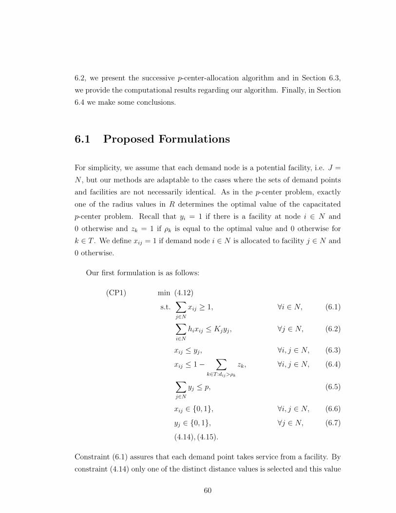
6.2, we present the successive p-center-allocation algorithm and in Section 6.3,

we provide the computational results regarding our algorithm. Finally, in Section

6.4 we make some conclusions.


For simplicity, we assume that each demand node is a potential facility, i.e. J =

N , but our methods are adaptable to the cases where the sets of demand points

and facilities are not necessarily identical. As in the p-center problem, exactly

one of the radius values in R determines the optimal value of the capacitated

p-center problem. Recall that yi = 1 if there is a facility at node i ∈ N and

0 otherwise and zk = 1 if ρk is equal to the optimal value and 0 otherwise for

k ∈ T . We define xij = 1 if demand node i ∈ N is allocated to facility j ∈ N and

0 otherwise.

Our first formulation is as follows:

(CP1) min (4.12)

s.t.∑j∈N

xij ≥ 1, ∀i ∈ N, (6.1)

∑i∈N

hixij ≤ Kjyj, ∀j ∈ N, (6.2)

xij ≤ yj, ∀i, j ∈ N, (6.3)

xij ≤ 1−∑

k∈T :dij>ρk

zk, ∀i, j ∈ N, (6.4)

∑j∈N

yj ≤ p, (6.5)

xij ∈ 0, 1, ∀i, j ∈ N, (6.6)

yj ∈ 0, 1, ∀j ∈ N, (6.7)

(4.14), (4.15).

Constraint (6.1) assures that each demand point takes service from a facility. By

constraint (4.14) only one of the distinct distance values is selected and this value

60

becomes the optimal objective value by objective function (4.12). Constraints

(6.2) ensure that the total demand assigned to any facility does not exceed its

capacity. Constraints (6.3) force that there is a facility at node j ∈ N if any

node is assigned to node j. Constraint (6.4) eliminates the assignments with

distance values greater than the selected optimal distance value and constraint

(6.5) restricts the number of facilities to p.

Our second formulation is as follows:

(CP2) min (4.12)

s.t.∑

j∈Nρk (i)

xij ≥ zk, ∀i ∈ N, k ∈ T, (6.8)

∑i∈Nρk (j)

hixij ≤ Kρkj yj, ∀j ∈ N, k ∈ T, (6.9)

(4.14), (4.15), (6.3), (6.5), (6.6), and (6.7)

Constraints (6.8) ensure that each demand node is assigned to a facility

within the selected radius value. One may question the validity of constraints

(6.9) in this model, we clear out this question as follows: since Kρkj =

minKj,∑

i∈Nρk (j) hi, constraints (6.9) can be expressed as∑

i∈Nρk (j) hixij ≤minKj,

∑i∈Nρk (j) hiyj,∀j ∈ N, k ∈ T . Then, we must have

∑i∈Nρk (j) hixij ≤

Kjyj and∑

i∈Nρk (j) hixij ≤∑

i∈Nρk (j) hiyj,∀j ∈ N, k ∈ T . The first expression

is valid since∑

i∈Nρk (j) hixij ≤∑

i∈N hixij ≤ Kjyj,∀j ∈ N, k ∈ T and the latter

one is valid due to constraints (6.3).

In this model, we can use constraints (6.2) of CP1 instead of constraints

(6.9), but we aim to have stronger inequalities by utilizing the effective ca-

pacities. For k = M , constraints (6.9) are equivalent to∑

i∈N hixij ≤(minKj,

∑i∈N hi)yj,∀j ∈ N and these constraints are stronger than constraints

(6.2) if∑

i∈N hi < Kj. Moreover, if we solve CP2 for a single radius value r, we

obtain much stronger constraints∑

i∈N hixij ≤ Krj yj, ∀j ∈ N by using the effec-

tive capacities. Therefore, we prefer presenting CP2 with constraints (6.9).

Constraints (6.8) in CP2 can be tightened as done in Chapter 4 and a new

mathematical formulation can be obtained by replacing constraints (6.8) with the

61

tightened ones given below:∑j∈Nρk (i)

xij ≥k∑l=1

zl, ∀j ∈ N, k ∈ T. (6.10)

The new formulation that we refer to as CP2T can be summarized as follows:

min (4.12)

s.t. (4.14), (4.15), (6.3), (6.5), (6.6), (6.7), (6.9), and (6.10).

We solve our models on the capacitated p-median data from OR-Library [15]. We

observe that CP2 performs better in terms of the average solution times and the

LP relaxation bounds of CP2T is larger.

By replacing constraints (6.6) with xij ≥ 0, ∀i, j ∈ N in CP1, CP2, or CP2T,

we can obtain mathematical formulations for solving the multiple allocation ca-

pacitated p-center problem that we focus on in Chapter 7. Note that the math-

ematical models in [57] and [58] cannot be adapted to the multiple allocation

p-center problem with the relaxation of x variables. Thus, our formulations have

an advantage in that sense.

The inequality∑i∈N

Kiyi ≥∑j∈N

hj is a valid inequality for our models. We can

replace this inequality with the following set of stronger inequalities:∑i∈N

Kρki yi ≥∑

j∈Nhjzk,∀k ∈ T .

In the capacitated p-center problems, the following issue needs attention. In

the general case of the problem, we assume that a facility which is also a demand

point can be assigned to a different facility. Because this allocation might provide

a better solution in terms of the optimal value and the restriction of allocating

each facility to itself might result in sub-optimal solutions. However, in some

applications of the problem, self-assignment might be compulsory for the facilities;

in such cases the addition of the constraint xii = yi, i ∈ N to our models handles

this requirement.

In the next section, we propose a new algorithm which is based on decompos-

ing the problem into two subproblems and solving them sequentially and repeat-

edly as needed.

62

6.2 Successive p-Center-Allocation Algorithm

This algorithm can be considered as a method that decomposes the capacitated

p-center problem into two subproblems and solves the subproblems iteratively

to obtain the optimal value of the original problem. Since this method can be

applied for both allocation strategies, we will refer to both problems when we

say capacitated p-center problem in this section unless it is stated explicitly.

The main method of the algorithm consists of two levels. In the first level, the

uncapacitated p-center problem is solved optimally and in the second level the

feasibility of this optimal solution in terms of viable allocations for the capacitated

p-center problem is checked. If the capacitated p-center problem is feasible, then

the current solution is an optimal solution for the capacitated p-center problem

as well; otherwise, the current solution is removed from the feasible region and

the uncapacitated p-center problem is solved for the updated feasible region. The

procedure is repeated until either a feasible solution is found for the capacitated p-

center problem or the uncapacitated p-center problem becomes infeasible implying

that the capacitated p-center problem is infeasible as well. Several versions for

the implementation of this algorithm can be discussed, but here we provide only

one version, of which we give the details below.

For an arbitrary k ∈ T with ρk = r, we solve the following model.

(UPk) min 0

s.t.∑

j∈Nr(i)

yj ≥ 1 ∀i ∈ N, (6.11)

∑j∈N

yj = p (6.12)

yj ∈ 0, 1 ∀j ∈ N

Decision variables and parameters in UPk are defined as in CP1 and CP2. If UPk

is infeasible, then we need to select a larger v ∈ T : v > k; otherwise, solving UPk

provides a feasible solution y and we check if the following allocation problem is

feasible for y and r.

63

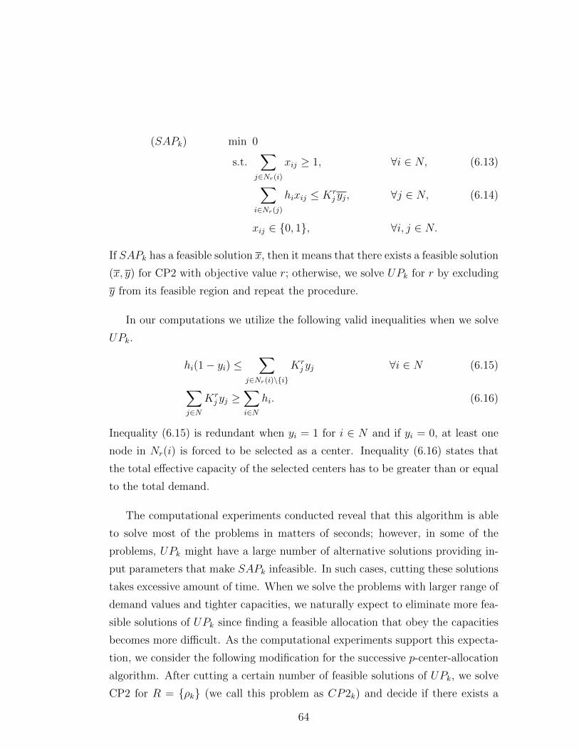
(SAPk) min 0

s.t.∑

j∈Nr(i)

xij ≥ 1, ∀i ∈ N, (6.13)

∑i∈Nr(j)

hixij ≤ Krj yj, ∀j ∈ N, (6.14)

xij ∈ 0, 1, ∀i, j ∈ N.

If SAPk has a feasible solution x, then it means that there exists a feasible solution

(x, y) for CP2 with objective value r; otherwise, we solve UPk for r by excluding

y from its feasible region and repeat the procedure.

In our computations we utilize the following valid inequalities when we solve

UPk.

hi(1− yi) ≤∑

j∈Nr(i)\i

Krj yj ∀i ∈ N (6.15)

∑j∈N

Krj yj ≥

∑i∈N

hi. (6.16)

Inequality (6.15) is redundant when yi = 1 for i ∈ N and if yi = 0, at least one

node in Nr(i) is forced to be selected as a center. Inequality (6.16) states that

the total effective capacity of the selected centers has to be greater than or equal

to the total demand.

The computational experiments conducted reveal that this algorithm is able

to solve most of the problems in matters of seconds; however, in some of the

problems, UPk might have a large number of alternative solutions providing in-

put parameters that make SAPk infeasible. In such cases, cutting these solutions

takes excessive amount of time. When we solve the problems with larger range of

demand values and tighter capacities, we naturally expect to eliminate more fea-

sible solutions of UPk since finding a feasible allocation that obey the capacities

becomes more difficult. As the computational experiments support this expecta-

tion, we consider the following modification for the successive p-center-allocation

algorithm. After cutting a certain number of feasible solutions of UPk, we solve

CP2 for R = ρk (we call this problem as CP2k) and decide if there exists a

64

feasible solution for the capacitated p-center problem for the current radius value

ρk. Then we select a larger radius value if CP2k is infeasible or a smaller radius

value if it is feasible. The details of our successive p-center-allocation algorithm

with the modifications mentioned above are provided in Algorithm 3.

Algorithm 3 Successive p-center-allocation Algorithm(BL)

ρ1 < ρ2 < . . . < ρM , min← 1, max←M , stop← false, OptV al←∞.1: while max−min ≥ 1 do2: mid← b(min + max)/2c,3: Create an empty cut set Q.4: while stop = false do5: if |Q| ≤MaxCutNumber then6: Solve UPmid with cuts in Q.7: if UPmid has a feasible solution y then8: Solve SAPmid for y.9: if SAPmid is feasible then

10: OptV al = ρmid,11: max← mid,12: stop← true.13: else14: Q← Q ∪ (

∑j∈N :yj=1

yj ≤ p− 1).

15: end if16: else17: min← mid+ 1,18: stop← true.19: end if20: else21: Solve CP2mid with cuts in Q.22: if CP2mid is feasible then23: max← mid,24: OptV al = ρmid.25: else26: min← mid+ 1,27: end if28: end if29: end while30: end while

65


We conduct experiments on three different data sets. The first data set is the

capacitated p-median data from OR-Library [15] and it consists of 10 instances

with n = 50, p = 5 and 10 instances with n = 100, p = 10. In this data, the

demand, capacity, and the location coordinates of each node is provided. The

capacity is identical for all nodes. From the coordinate locations, we calculate

the Euclidean distance between each node pair and round it down to the nearest

integer. Although the triangular inequality is ruined by rounding, we remain safe

since we do not require this property in our methods. In the rest of this section,

we call this data as D1. The second data set is taken from [66] and it is a real

data corresponding to the central area of Sao Jose dos Campos city. In this data,

n varies from 100 to 402 and p varies from 10 to 40. We refer to this data as D2.

In D2, the capacities of the facilities are identical in each single problem instance.

We create a third data set, D3, by using pmed21, pmed26, pmed31, pmed35, and

pmed38 networks of the uncapacitated p-median data set from OR-Library [15].

In D3, we construct three instances for each network with p = 5, 10, and n/10.

We generate demand values uniformly between 1 and 500 and capacity values

uniformly between 1 and 2d∑

j∈N hj108pe.

When we solve the capacitated p-center problem with any of the methods

we propose, we utilize the optimal value of the uncapacitated p-center problem

as the lower bound for the optimal value. To obtain an upper bound value for

the single allocation capacitated p-center problem, we define two methods; one

of them is for the problems with identical capacities and the other one works for

the ones with non-identical capacities.

• General capacities: Let Fmax be the set of p facilities with largest capacities

and F (i) = j ∈ Fmax : hi ≤ Kj. Then, maxj∈N maxj∈F (i) dij is an upper

bound for the single allocation capacitated p-center problem.

• Equal capacities: Let Ti = maxj∈N dij, i ∈ N and Ti1 ≤ Ti2 ≤ . . . ≤ Tin .

Then, Tin−p+1 is an upper bound for the single allocation capacitated p-

center problem. This upper bound can be improved by comparing Ti values

66

with the second largest distance values to i ∈ N .

The times spent to obtain these lower and upper bounds are included in the

solution times reported in the tables throughout this chapter. We compare the

computational performance of our algorithm with the binary search algorithm

given in Algorithm 4. In this binary search algorithm, we solve our formulation

CP2k.

Algorithm 4 Binary Search Algorithm(BS)

ρ1 < ρ2 < . . . < ρM , min← 1, max←M , OptV al←∞.1: while max−min ≥ 1 do2: mid← b(min + max)/2c,3: Solve CP2mid.4: if CP2mid is feasible then5: OptV al = ρmid,6: max← mid.7: else8: min← mid+ 1.9: end if

10: end while

Tables 6.1-6.3 give the results for solving the single allocation capacitated p-

center problem by using the binary search and the successive p-center-allocation

algorithms on data sets D1, D2, and D3, respectively. In these tables, the columns

under n, p, and Opt gives the numbers of nodes, number of facilities to be placed,

and the optimal values of the problems, respectively. The columns under LB

and UB show the lower and upper bound values introduced to the algorithms

while solving the problems and the last two columns give the total solution times

including the times needed to obtain the lower and upper bounds for the two

algorithms.

From Table 6.1, we observe that in terms of the solution times, the two algo-

rithms are not much different from each other, but binary search performs slightly

better than the successive p-center-allocation algorithm not only on the average

but also on the worst case.

Table 6.2 gives the results for solving the single allocation capacitated p-center

67

Table 6.1: Solution times (seconds) of binary search and successive p-center-allocation algorithms on D1 instances for the single allocation capacitated p-center problem

Binary Search Successive p-center-allocationn p LB UB Opt Times Times

50 5 29 82 29 0.95 0.7650 5 31 77 33 0.76 0.6250 5 26 72 26 0.64 0.3650 5 31 70 32 0.92 1.0950 5 27 66 29 0.64 1.0250 5 28 76 31 1.28 4.0250 5 30 70 30 1.04 0.7550 5 29 81 31 0.80 1.4850 5 27 70 28 0.87 1.7850 5 29 76 32 0.88 0.65

100 10 19 69 19 3.94 3.94100 10 19 75 20 3.48 6.33100 10 19 80 20 5.08 3.39100 10 20 76 20 5.10 2.15100 10 20 79 21 4.96 3.64100 10 19 70 20 6.29 8.12100 10 20 74 22 21.57 31.35100 10 19 76 21 6.88 6.00100 10 20 75 21 4.35 13.73100 10 18 84 21 8.32 19.52

Avg.: 3.94 5.54

68


Binary Search Successive p-center-allocationn p LB UB Opt Times Times

100 10 316 1488 364 18.02 54.46100 15 301 1631 304 18.69 30.66300 25 276 1995 278 113.97 69.41300 30 245 2034 253 78.13 59.62402 30 277 2150 284 465.32 309.85402 40 238 2214 239 373.34 350.63

Avg.: 177.91 145.77

problem on D2 instances by using the successive p-center-allocation algorithm and

the binary search algorithm. In this table, the solution times of the successive

p-center-allocation algorithm are smaller than the solution times of the binary

search algorithm for all instances except the first instance. Another observation

on this table is that the average and the worst solution times of the successive

p-center-allocation algorithm are better than those of the binary search algorithm

on this data. The worst solution time of the successive p-center-allocation algo-

rithm is 350.63 seconds while it is 465.32 seconds for the binary search algorithm.

The average solution time of the binary search algorithm is 177.91 seconds and

it is 145.77 seconds for the successive p-center-allocation algorithm.

Table 6.3 presents the results that we obtain from solving the single allocation

capacitated p-center problem by the binary search and the successive p-center-

allocation algorithms on D3 instances. In this table, we observe that all problems,

except for one, are solved much faster by the successive p-center-allocation algo-

rithm. Only the problem with n = 600 and p = 60 is solved around three times

faster by the binary search algorithm. For two of the instances in this table, no

solution can be found within 10 hours by using the binary search algorithm (so,

the algorithm is interrupted after 10 hours); the average and the worst solution

times of the remaining instances are 9934.03 seconds and 38376.68 seconds, re-

spectively. The average and the worst solution times of all instances are 327.82

seconds and 3314.96 seconds, respectively, for the successive p-center-allocation

69


Binary Search Successive p-center-allocationn p LB Opt Times Times

500 5 40 40 8979.08 9.24500 10 34 34 2253.20 7.13500 50 22 22 209.67 73.45600 5 38 38 14257.20 19.25600 10 32 32 9891.35 11.04600 60 19 19 380.14 1183.39700 5 30 30 9692.34 11.63700 10 27 27 19939.28 9.89700 70 15 19 472.21 77.22800 5 30 30 38376.68 22.19800 10 26 26 11152.76 19.78800 80 14 21 2922.31 115.74900 5 29 29 NA 19.60900 10 24 24 NA 22.84900 90 12 24 10616.13 3314.96

Avg.: 9934.03 327.82

algorithm. Another observation that we obtain from this table is that, the binary

search algorithm solves the instances with p = n/10 faster while the successive

p-center-allocation algorithm solves problems with p = 5 or p = 10 faster for the

same n values with the same network. In this table, the upper bound values are

equal to the largest distance value; therefore, we do not give them explicitly.

6.4 Conclusion

In this chapter, we presented new mathematical formulations and a successive

p-center-allocation algorithm to solve the single allocation capacitated p-center

problem. We conducted large scale experiments on three different data sets;

two of them were available in the literature for solving the capacitated p-median

data and used for solving the capacitated p-center problem in previous studies.

70

We created the other one by using the uncapacitated p-median data from OR-

Library [15]. We compared the performance of our successive p-center-allocation

algorithm with a binary search algorithm over distinct radius values that solves

one of our mathematical models for the selected fixed radius value at each step.

We observed that the successive p-center-allocation algorithm performs better in

terms of the solution times especially in larger problems when compared to the

binary search algorithm. We were able to solve problems with up to 900 nodes

by using our successive p-center-allocation algorithm.

The methods we proposed in this chapter are readily adaptable to the multiple

allocation capacitated p-center problem. We leave the details of this adaptation

to Chapter 7.

71

Chapter 7

A Branch and Cut Algorithm for

Solving the Multiple Allocation

Capacitated p-Center Problem

The multiple allocation capacitated p-center problem did not receive any atten-

tion in the literature. When we consider the school districting problem or medical

units location problem, allocating the demand of a district to distinct facilities

is meaningful and this type of allocation provides solutions as good as the ones

obtained from the single allocation version in terms of the worst case service

level. Therefore, it is worth to study the multiple allocation capacitated p-center

problem. The mathematical models and the successive p-center-allocation algo-

rithm that we propose for the single allocation capacitated p-center problem solve

the multiple allocation capacitated p-center problem when the binary restriction

of the x variables in these methods is removed. By changing x variables with

ω : ωij = hixij,∀i, j ∈ N variables, we can obtain three additional formulations

for the multiple allocation capacitated p-center problem. In the next section,

we explicitly present a formulation called MCP2, which is the relaxed version of

CP2, and another formulation called MCPW2, which is obtained from MCP2 by

changing x variables with ω variables. Other than these methods, we propose

a new branch and cut algorithm for the multiple allocation capacitated p center

72

problem. We give the details of our branch and cut algorithm in Section 7.2 and

the experimental results that we obtained by using our branch and cut algorithm

in Section 7.3.


The parameters that are used in this section and the decision variable y is as

defined in Chapter 6. Let xij be the fraction of demand of node i ∈ N satisfied

by facility j ∈ N .

(MCP2) min (4.12)

s.t. (4.14), (4.15), (6.3), (6.5), (6.6), (6.7), (6.8), (6.9),

xij ≥ 0,∀i, j ∈ N. (7.1)

If we place ωij instead of hixij in MCP2, we obtain the following formulation:

(MCPW2) min (4.12)

s.t.∑

j∈Nρk (i)

ωij ≥ hizk, ∀i ∈ N, k ∈ T, (7.2)

∑i∈Nρk (j)

ωij ≤ Kρkj yj, ∀j ∈ N, k ∈ T, (7.3)

ωij ≤ hiyj, ∀i, j ∈ N, (7.4)

ωij ≥ 0, ∀i, j ∈ N, (7.5)

(4.14), (4.15), (6.5), and (6.7).

We can make this type of change in other models that are relaxations of CP1

and CP2T as well. The computational experiments we conducted on problems

with small sizes revealed that among six models, MCP2 provides the best perfor-

mance in terms of the solutions times.

73

7.2 A Branch and Cut Algorithm

When we consider the mathematical formulation MCP2 for a fixed radius value

r, the model turns into a feasibility problem. Then, we can use∑

j∈N yj or any

constant (say 0) as the objective function. Below we give an appropriate formu-

lation of this problem. As pointed out in Section 6.1, we disregard constraints

(6.3) of CP2 without effecting the feasible region of the problem.

(FMCP) min 0 (7.6)

s.t.∑

j∈Nr(i)

xij ≥ 1, ∀i ∈ N (7.7)

∑i∈Nr(j)

hixij ≤ Krj yj ∀j ∈ N (7.8)

(6.5), (6.7), and (7.1).

By projecting out the nonnegative x variables in FMCP, we obtain a new formu-

lation with an exponential number of constraints and we develop a branch and

cut algorithm to solve this new formulation by adding the constraints iteratively

as they are needed. For the projection, we consider the locations of the facilities

as fixed and take the dual. Let πi, i ∈ N be the dual variables associated with

constraints (7.7) and uj, j ∈ N be the dual variables associated with constraints

(7.8), then the dual problem can be expressed as follows:

(DP) max∑i∈N

πi −∑j∈N

Krj yjuj (7.9)

s.t. πi − hiuj ≤ 0, ∀i, j ∈ N : dij ≤ r (7.10)

πi ≥ 0, ∀i ∈ N (7.11)

uj ≥ 0, ∀j ∈ N. (7.12)

Then, we analyze the extreme rays of the feasible region of the dual problem. Let

us denote the feasible region of DP with W and define Nr(S) =⋃i∈S

Nr(i) for any

set S ⊆ N . The following proposition reveals the characterization of the extreme

rays of W .

Proposition 3. Let (π, u) 6= 0 be a solution to W , then it is an extreme ray of

W if and only if it satisfies the following conditions:

74

1. ui ∈ 0, 1,∀i ∈ N and πi = hi or 0, ∀i ∈ N .

2. Let S = i ∈ N : ui > 0 and S∗ = i ∈ N : πi > 0. Either |S| = 1 or

∀i ∈ S Nr(i) ∩ S∗ 6= ∅.

3. For any S∗1 ⊂ S∗, Nr(S∗1) ∩Nr(S

∗ \ S∗1) 6= ∅.

Proof. (Sufficiency:) Suppose (π, u) ∈ W is not an extreme ray of W . Then,

there exist two rays (π, u)1 and (π, u)2 that satisfies

(i) (π, u)1, (π, u)2 ∈ W ;

(ii) neither (π, u)1 nor (π, u)2 is equivalent to (π, u); and

(iii) 12(π, u)1 + 1

2(π, u)2 = (π, u).

Note that (π, u)1, (π, u)2 ≥ 0 due to (i); thus, (πi)1 = (πi)

2 = 0 for i ∈ N : πi = 0

and (uj)1 = (uj)

2 = 0 for j ∈ N : uj = 0 from (iii).

Now, suppose (π, u) satisfies 1, 2, and 3. Since (π, u)1 is not equivalent to

(π, u), there exits i ∈ N such that either (πi)1 6= πi or (ui)

1 6= ui. In order

to avoid complication, let us assume that (π1)1 6= π1 (note that we can do this

without loss of generality). Then, either (π1)1 = π1− ε or (π1)1 = π1 + ε for some

sufficiently small ε > 0.

Let us consider the case where (π1)1 = π1− ε, note that the case with (π1)1 =

π1 + ε follows similarly. From (i), we have h1− ε ≤ h1(uj)1 and h1 + ε ≤ h1(uj)

2,

∀j ∈ Nr(1) ⇒ h1 − ε ≤ h1 minj∈Nr(1)(uj)1 and h1 + ε ≤ h1 minj∈Nr(1)(uj)

2.

Using (iii), we have 1 + εh1≤ minj∈Nr(1)2 − (uj)

1 or equivalently 1 + εh1≤

2−maxj∈Nr(1)(uj)1. Since 1− ε

h1≤ minj∈Nr(1)(uj)

1 and 1− εh1≥ maxj∈Nr(1)(uj)

1,

(uj)1 = 1 − ε

h1and (uj)

2 = 1 + εh1, ∀j ∈ Nr(1). Then by (i) and (iii), (πj)

1 =

hj(1− εh1

) and (πj)2 = hj(1 + ε

h1),∀j ∈ Nr(1).

Now, if S∗\(Nr(1)∩S∗) = ∅, then every positive entry of (π, u)1 and (π, u)2 is

multiplied by (1− εh1

) and (1+ εh1

), respectively, since S∗ ⊆ Nr(1) and S ⊆ Nr(S∗)

by 2 and this implies that (π, u) is an extreme ray of W .

75

If S∗\(Nr(1)∩S∗) 6= ∅, then ∃k ∈ S∗\(Nr(1)∩S∗). Due to 3, Nr(1)∩Nr(S∗\

1) 6= ∅, so, Nr(1) ∩ Nr(k) 6= ∅. Then, by (i) and (iii), (πk)1 = hk(1 − ε

h1),

(πk)2 = hk(1 + ε

h1), (uk)

1 = 1 − εh1

, and (uk)2 = 1 + ε

h1. This implies that

(πi)1 = hi(1− ε

h1), (πi)

2 = hi(1+ εh1

), (ui)1 = 1− ε

h1, and (ui)

2 = 1+ εh1,∀i ∈ Nr(k).

Now, if S∗\((Nr(1)∪Nr(k))∩S∗) = ∅, then every positive entry of (π, u)1 and

(π, u)2 is multiplied by (1− εh1

) and (1 + εh1

), respectively, and this implies that

(π, u) is an extreme ray of W otherwise, we consider the partition S∗1 = 1, kand S∗ \ S∗1 and repeat arguments. At each iteration we multiply at least one

πi and one ui entry of (π, u)1 and (π, u)2 by (1 − εh1

) and (1 + εh1

), respectively.

Finally, we end up with S∗ \ (⋃i∈S∗1

Nr(i) ∩ S∗) = ∅ and conclude that (π, u) is an

extreme ray of W .

Now, suppose (π)1 = (π)2 = π but (u1)1 6= u1. Then, either 0 ≤ (u1)1 < 1

or (u1)1 > 1. If (u1)1 < 1, then, (πj)1 ≤ hj(u1)1 < hj = πj for some j ∈ S∗

by (i), which contradicts with (π)1 = (π)2 = π. If (u1)1 > 1, then (u1)2 < 1

and (πj)2 ≤ hj(u1)2 < hj = πj for some j ∈ S∗ by (i) which contradicts with

(π)1 = (π)2 = π.

Thus, we can conclude that (π, u) is an extreme ray of W if it satisfies prop-

erties 1, 2, and 3.

(Necessity:)

1. Suppose that 1 = ui1 = ui2 = . . . = uik < uik+1= 1 + δ ≤ . . . ≤ uin . In this

case, there exist solutions (π, u)1, (π, u)2 ∈ W such that

(ui1)1 = . . . = (uik)1 = 1− δ/2,

(ui1)2 = . . . = (uik)2 = 1 + δ/2,

(πj)1 = (1− δ/2)πj,

(πj)2 = (1 + δ/2)πj, ∀j ∈

⋃q=1,...,k

Nr(iq),

(πj)1 = (πj)

2 = πj, ∀j /∈⋃

q=1,...,k

Nr(iq),

(uj)1 = (uj)

2 = uj, j = ik+1, . . . , in.

76

Then, we have 12(π, u)1 + 1

2(π, u)2 = (π, u) implying that (π, u) is not

an extreme ray of W . Therefore, we must have uj = 1,∀j ∈ S and

uj = 0, ∀j ∈ N \ S for some nonempty S ⊂ N .

Moreover, note that πi = 0, ∀i ∈ N \ S∗ is required for feasibility of (π, u).

Now, suppose to the contrary that πk = hk − γ for sufficiently small γ > 0

for some k ∈ N . Then, there exist (π, u)1, (π, u)2 ∈ W such that

(πk)1 = πk − γ/2,

(πk)2 = πk + γ/2,

(πj)1 = (πj)

2 = πj, j 6= k,

u1 = u2 = u.

Then, (π, u)1 6= (π, u), (π, u)2 6= (π, u), and 12(π, u)1 + 1

2(π, u)2 = (π, u)

which implies that (π, u) cannot be an extreme ray.

2. Suppose Nr(κ) ∩ S∗ = ∅ for some κ ∈ S : |S| ≥ 2. We can construct

(π, u)1, (π, u)2 ∈ W such that

(uκ)1 = uκ(1− ε),

(uκ)2 = uκ(1 + ε),

(ui)1 = (ui)

2 = ui, ∀i ∈ N \ κ, and

(π)1 = (π)2 = π.

Since |S| ≥, (π, u)1 6= (π, u) and (π, u)2 6= (π, u). Since 12(π, u)1 + 1

2(π, u)2 =

(π, u), (π, u) cannot be an extreme ray.

3. Suppose ∃S∗1 ⊂ S∗ such that Nr(S∗1) ∩Nr(S

∗ \ S∗1) = ∅. Now, consider the

77

following setting of (π, u)1 and (π, u)2:

(πi)1 = hi(1− ε)ui,

(πi)2 = hi(1 + ε)ui,

(ui)1 = (1− ε)ui, and,

(ui)2 = (1 + ε)ui, 0 < ε < 1, ∀i ∈ Nr(S

∗1),

(πj)1 = (πj)

2 = πj, ∀j ∈ Nr(S∗ \ S∗1),

(uj)1 = (uj)

2 = uj, ∀j ∈ Nr(S∗ \ S∗1).

Obviously, (π, u)1 6= (π, u) and (π, u)2 6= (π, u). Since 12(π, u)1 + 1

2(π, u)2 =

(π, u), (π, u) cannot be an extreme ray.

We proved that any (π, u) ∈ W is an extreme ray of W if and only if it satisfies

properties 1, 2, and 3.

By projecting out the x variables from FMCP, we obtain the following equiv-

alent model for fixed radius value:

(MP) min 0 (7.13)

s.t.∑i∈S

Kri yi ≥

∑i∈S∗

hi ∀S∗, S ⊆ N with properties in Proposition 3

(7.14)

(6.5) and (6.7)

In this model, constraints (7.14) ensure that the total capacity of the nodes in S

is no less than the total demand of the nodes in S∗. In other words, the demand

of the nodes which have no connection with outside of S has to be served by the

nodes in S. In our computations, we choose minimizing∑

j∈N yj in the objective

function and utilize the valid inequalities (6.15) and (6.16).

hi(1− yi) ≤∑

j∈Nr(i)\i

Krj yj ∀i ∈ N (6.15)

∑j∈N

Krj yj ≥

∑i∈N

hi. (6.16)

78

In our branch and cut algorithm, we solve the following strengthened LP for

the separation of inequalities (7.14).

(SP) max (7.9)

s.t. (7.10), (7.11), (7.12),

uj ≤∑

i∈Nr(j)

πi, ∀j ∈ N (7.15)

uj ≤ 1, ∀j ∈ N (7.16)

In this separation model, we aim to obtain solutions that provide positive objec-

tive values. Constraints (7.15) eliminate the extreme rays with S∗ = ∅, |S| = 1.

Since the objective values of this sort of extreme rays are non-positive, we do not

lose generality with the addition of constraints (7.15) to our separation model.

Let (π, u) be the optimal solution obtained from SP. If the optimal value of this

solution is 0, then it means that all of constraints (7.14) in the master problem

are satisfied. If the optimal value is positive, then we find a violated constraint

associated with S, S∗ pair where S = i ∈ N : ui = 1 and S∗ = i ∈ N : πihiand add this constraint to MP.

In order to decide on the optimal value of the multiple allocation capacitated

p-center problem, we need to solve the master problem for a finite series of radius

values. For this purpose, we use the binary search strategy as in the successive

p-center-allocation algorithm.


We conduct experiments on two different data sets. The first one is D3 of Chapter

6 and the second one, which we call as D4, is from d1291 data of TSPLIB [16].

In D4, we have 5 instances with p = 5, 10, 100, 129, and 500. In d1291, the

location coordinates of each node is given. We calculate the Euclidean distance

between each node pair and round it down to the nearest integer. As in D3,

we generate demand values uniformly between 1 and 500 and capacity values

uniformly between 1 and 2d∑

j∈N hj108pe.

79

We can obtain an upper bound for the multiple allocation p-center problem

as follows: We solve FMCP for any radius value by setting yj = 1, ∀j ∈ Fmax,

where Fmax is the set of p facilities with largest capacities, and decide if there

exists a feasible solution for that radius value. By using a search strategy, such as

binary search or the ones given in Chapter 4, we are able to decide on the smallest

radius value that provides a feasible solution with facility set Fmax in polynomial

time. This smallest radius value is an upper bound for the multiple allocation

capacitated p-center problem. We utilize this upper bound in our computations

for solving the multiple allocation capacitated p-center problem. As in the single

allocation case, we utilize the optimal value of the uncapacitated p-center problem

as the lower bound. The times spent on obtaining the lower and upper bounds

are included in the solution times reported in the tables.

In Table 7.1, we compare the performance of our successive p-center-allocation

and branch and cut algorithms for solving the multiple allocation capacitated p-

center problem on D3 instances. From this table, we observe that the successive

p-center-allocation algorithm performs better in terms of the solution times on

the instances with p = 5 and p = 10 while the branch and algorithm performs

better on the instances with p = n/10. When we look at the average solution

times of these algorithms, we see that it is 118.13 seconds for the successive p-

center-allocation algorithm and 28.84 seconds for the branch and cut algorithm.

Moreover, the worst solution time of the successive p-center-allocation algorithm

is 1226.16 seconds while it is 65.94 seconds for the branch and cut algorithm.

Therefore, we can conclude that the branch and cut algorithm performs much

better both on the average and worst case on this data set.

We solve problems in D4 by using our branch and cut algorithm and give the

results in Table 7.2. We are able to solve problems with p = 5 and 10 optimally

in less than 2 minutes. However, we are not able to solve the problems with

p = 100, 129 and 500 optimally within the 1 hour limitation. The gap between

the best upper and lower bounds we obtained for these problems are greater than

100%. The average time to solve the first two instances is 99.45 seconds.

From our experiments on D4, we observe that in our branch and cut algorithm

80

Table 7.1: Solution times (seconds) of our algorithms on D3 instances for themultiple allocation capacitated p-center problem

Successive p-center-allocation Branch and Cutn p LB UB Opt Times Times

500 5 40 54 40 8.80 16.88500 10 34 50 34 6.64 16.42500 50 22 41 22 47.58 32.74600 5 38 53 38 19.87 27.77600 10 32 53 32 9.84 19.31600 60 19 41 19 64.66 25.15700 5 30 44 30 11.20 26.77700 10 27 38 27 9.84 19.39700 70 15 31 19 98.89 45.37800 5 30 40 30 22.15 23.29800 10 26 36 26 16.93 36.96800 80 14 31 21 177.93 13.10900 5 29 59 29 23.03 37.79900 10 24 56 24 28.45 65.94900 90 12 44 24 1226.16 25.79

Avg.: 118.13 28.84

Table 7.2: Solution times (seconds) of our Branch and Cut Algorithm on D4instances for the multiple allocation capacitated p-center problem

n p LB UB Opt Time

1291 5 1007 1805 1010 82.991291 10 594 1487 594 115.911291 100 127 1390 NA NA1291 129 114 1510 126 NA1291 500 50 216 NA NA

Avg.: 99.45

81

MP model is solved faster for larger radius values, but it might take large amount

of time to solve MP for small radius values. If we try to solve MP with branch

and cut for large radius values and CP2k instead of MP for smaller radius values,

we are able to obtain the optimal value for problem with p = 129 in less than

half an hour by limiting the branch and cut time with 2 minutes; but, we are not

able to solve problem with p = 100 within a reasonable time limit since CP2k

takes more than 3 hours to solve for some radius values.

82

Chapter 8

Conclusions and Future Research

Directions

8.1 Preliminary Results of a Benders Decom-

position Algorithm for Solving the p-Center

Problem

In order to handle difficult problems more easily, several decomposition methods

are available in the literature. In this section, we focus on solving the p-center

problem by using the Benders Decomposition method [67]. This method can be

applied to the models that have a certain structure and we are able to formulate

the p-center problem in such a way. We initially give the details of our mathe-

matical formulation and then, go into the details of our Benders Decomposition

algorithm. We present our method for the vertex restricted p-center problem,

but, it can easily be adapted to the absolute p-center problem. Let xij be the

amount of flow going from node i ∈ N to facility j ∈ J . Define y and z variables

as in Chapter 4. Then, the following mathematical model solves the p-center

problem optimally.

83

(BP) min (4.12)

s.t.∑

j∈Nρk (i)

xij ≥ zk, ∀i ∈ N, k ∈ T, (8.1)

xij ≥ 0 ∀i ∈ N, j ∈ J, (8.2)

(4.4), (4.5), (4.6), (4.14), and (4.15).

We can solve this model by decomposing into smaller problems as we discuss

in Chapter 4. Therefore, we can initially focus on solving BP for a single r ∈ R.

In this restrictive model, we make a simple modification by removing constraint

(4.5) and minimizing∑

j∈N yj in the objective. The modified restriction is as

follows:

(FBP) : min∑j∈J

yj (8.3)

s.t.∑

j∈Nr(i)

xij ≥ 1, ∀i ∈ N, (8.4)

(4.4), (4.6), and (8.2).

When the y variables are fixed to y in this model, we obtain a linear pro-

gramming problem. The dual problem of this linear programming problem can

be expressed as follows. We define α to be the set of dual variables associated

with constraints (8.4) and β to be the set of variables associated with constraints

(4.4).

(DF) : max∑j∈J

αi −∑i∈N

∑j∈Nr(i)

βijyj, (8.5)

s.t. αi − βij ≤ 0, ∀i ∈ N, j ∈ J : dij ≤ r, (8.6)

αi ≥ 0, ∀i ∈ N, (8.7)

βij ≥ 0, ∀i ∈ N, j ∈ J : dij ≤ r. (8.8)

This dual problem DF always has a feasible solution (α, β) = (0, 0) and this

solution is an extreme point of DF. Let (α, β)1 6= (0, 0) be any feasible solution for

84

DF, then, (α, β)2 = 2(α, β)1) is also feasible for DF and since 12(0, 0) + 1

2(α, β)2 =

(α, β)1, (α, β)1 cannot be an extreme point of DF. Thus, (0, 0) is the unique

extreme point of DF. Let (α, β)1, . . . , (α, β)K be the set of extreme rays of of

DF. The Benders reformulation for FBP can be expressed as follows:

(BR) : min z (8.9)

s.t. z ≥∑j∈J

yj, (8.10)

∑i∈N

αki −∑i∈N

∑j∈Nr(i)

βkijyj ≤ 0, k = 1, . . . , K, (8.11)

yj ∈ 0, 1 ∀j ∈ J.

Since the number of extreme rays of DF can be excessive, we develop a cutting

plane algorithm to solve the Benders reformulation. A typical repetitive step of

our algorithm can be described as follows: We solve DF by using the known y

values. If the problem is unbounded, we solve a modified dual problem MDF,

which has the same feasible region with DF but a constant objective function,

say ‘1’ and obtain an (α, β)1 solution, which is an extreme ray of DF. We solve

BR by adding the constraint associated with this extreme ray and obtain a new

(y)1 solution. We solve DF by using (y)1 values and repeat previous steps if DF is

unbounded. We terminate the algorithm when DF is bounded. The last solution

we obtained from BR is an optimal solution for FBP. If the optimal value of the

BR algorithm is greater than p, we can conclude that there exists no feasible

solution to FBP for the current radius value. Then, we choose a larger radius

value to solve FBP with the Benders algorithm.

Recall that the optimal value of the p-center problem is equal to one of the

distinct distance values R = ρ1, . . . , ρM. Therefore, we can solve the p-center

problem by using the binary search algorithm given in Chapter 4 except that we

solve BR for the corresponding element of R at each step instead.

We solve 40 instances of the uncapacitated p-median data from OR-Library

[15] by using our Benders Decomposition algorithm and compare with the double

85

bound algorithm. We observe that the Benders algorithm does not perform as

good as the double bound algorithm in terms of the solution times. On the other

hand, we observe that the solution times of the individual problems DF, MDF,

and BR of the Benders algorithm are quite small (less than 1 second). Therefore,

we try to solve some of the larger problems that cannot be solved by the double

bound algorithm within the time limit. For example, we know that the optimal

value of the problem with n = 2500 and p = 100 is between 1050 and 1059 from

Table 4.9. We try to solve FBP for r = 1054 by using the Benders algorithm.

During this experiment, the algorithm terminates due to memory overflow after

135 iterations and the last BR solved in this experiment provides an optimal value

of 64. Since each of the problems DF, MDF, and BR can be solved in less than

2 seconds, we believe that this memory overflow occurs not due to the size of

the models but due to programming related issues. Therefore, Benders algorithm

might be developed into a promising method for solving large problems in the

future.

8.2 Contribution Summary

In this thesis, we studied the p-center problem and the capacitated p-center prob-

lem on general networks with generalized settings. We approached these problems

from a modeling and algorithmic perspective. We concentrated on both absolute

and vertex restricted p-center problems on weighted and unweighted networks.

We investigated the capacitated p-center problem with both single and multiple

allocation strategies. Our studies on the multiple allocation capacitated p-center

problem are the first ones in the literature.

We developed new mathematical formulations and algorithms that solve both

absolute and vertex restricted p-center problems optimally. We obtained the

tightest lower bound from a semi-relaxation of our mathematical formulations.

One of our formulations provided the largest LP relaxation bound among the

existing formulations in the literature. In the experimentation phase, we ini-

tially focused on the vertex restricted p-center problem. For the vertex restricted

86

problem, we provided new upper and lower bounds that can be obtained via a

polynomial algorithm in no matter of time. These bounds are within a constant

multiple of the optimal value of the problem. We conducted large scale experi-

ments on both weighted and unweighted problems and solved problems with up to

3038 nodes. We observed that the weighted problems can be solved much faster

when compared to the unweighted problems. Since the symmetry of the distance

matrix is lost in the weighted version of the problem, the number of non-zero

coefficients decreases for a significant number of radius values. Therefore, solving

weighted problems in smaller computation times was in fact an expected result.

In order to solve the absolute p-center problem on the same networks, we needed

to generate the intersection points. For this purpose, we developed a method

for generation of the intersection points. In this method, we utilized the new

lower and upper bounds that we proposed specifically for the absolute p-center

problem. We were able to solve problems with up to 900 nodes and 16056 edges.

The largest solution time required was less than 509 seconds in our experiments.

As in our studies for the p-center problem, we initially focused on the mod-

eling approaches in solving the capacitated p-center problem. Then we directed

our attention to developing more effective algorithms that solve the problem op-

timally. We proposed several new mathematical formulations and a successive

p-center-allocation algorithm to solve both the single and multiple allocation ca-

pacitated p-center problems. The first set of our experiments were on the single

allocation version of the problem and we were able to solve problems with up to

900 nodes. Later, we developed a branch and cut algorithm to solve the multiple

allocation capacitated p-center problem and conducted experiments on relatively

larger sized problems with tight and loose, identical and non-identical capaci-

ties. We were able to solve problems with up to 1291 nodes by using our branch

and cut algorithm. In our experimentations, we utilized the optimal value of

the (uncapacitated) p-center problem as a lower bound for the optimal value of

the single and multiple allocation capacitated p-center problems. We also used

distinct upper bounds for solving the single and multiple allocation versions of

the problem.

87

8.3 Future Research Directions

One future improvement for our study on the capacitated p-center problem might

be to try to solve larger problems by utilizing the reduction rules that we used for

solving the p-center problem. Applying these rules improved the solution times

and best bounds obtained for several problems in Chapter 4. One may also think

of applying these rules for solving the absolute p-center problem. In this case,

since the allocation matrix of the absolute p-center problem is larger compared to

the one in the vertex restricted p-center problem, it is expected to come up with

larger reduction times. However, it might be worthy if CPLEX solution times

can be decreased enormously with the help of reduction process.

Another future research direction is to extend our methods for the p-center

problem to the fault tolerant p-center problem. The fault tolerant p-center prob-

lem is a generalization of the p-center problem, where each demand node must

have at least α centers close to it. The main motivation of this problem is to

establish a back-up option in case of failure of a center in providing service. Fault

tolerance can be studied in the capacitated p-center problem as well. In ad-

dition, one may wish to add some stochastic parameters to represent the fault

probabilities and minimize the maximum expected service time of demand nodes.

As revealed in the literature review, there are several studies of the p-center

problem on tree networks. However, the studies that focus on the capacitated p-

center problem on tree networks is restricted to a unique study on the balanced p-

center problem. Therefore, analyzing the structural properties of the generalized

capacitated p-center problem on special networks is an open research area.

Recent natural disasters attracted the attention of the researchers for focusing

on the evacuation planning problems. One of the main concerns of the evacuation

process is that people get stuck at the roads due to overloads and either it causes

a big chaos or evacuation cannot be achieved on time. These overloads can be

avoided if the capacities of the roads can be successfully utilized in the evacuation

plan. The affected population can be directed to the safe regions that will be

decided by solving a p-center problem with arc capacities.

88

Bibliography

[1] S. Elloumi, M. Labbe, and Y. Pochet, “A new formulation and resolution

method for the p-center problem,” INFORMS Journal on Computing, vol. 16,

no. 1, pp. 84–94, 2004.

[2] E. Minieka, “The m-center problem,” SIAM Review, vol. 12, no. 1, pp. 138–

139, 1970.

[3] K. Aardal, Y. Pochet, and L. A. Wolsey, “Capacitated facility location: valid

inequalities and facets,” Mathematics of Operations Research, vol. 20, no. 3,

pp. 562–582, 1995.

[4] S. L. Hakimi, “Optimum locations of switching centers and the absolute

centers and medians of a graph,” Operations Research, vol. 12, no. 3, pp. 450–

459, 1964.

[5] O. Kariv and S. L. Hakimi, “An algorithmic approach to network location

problems. Part I: The p-centers,” SIAM Journal on Applied Mathematics,

vol. 37, no. 3, pp. 513–538, 1979.

[6] J. Hooker, R. Garfinkel, and C. Chen, “Finite dominating sets for network

location problems,” Operations Research, vol. 39, no. 1, pp. 100–118, 1991.

[7] N. Christofides and P. Viola, “The optimum location of multi-centres on a

graph,” Operational Research Quarterly, pp. 145–154, 1971.

[8] C. Toregas, R. Swain, C. ReVelle, and L. Bergman, “The location of emer-

gency service facilities,” Operations Research, vol. 19, no. 6, pp. 1363–1373,

1971.

89

[9] R. Garfinkel, A. Neebe, and M. Rao, “The m-center problem: Minimax

facility location,” Management Science, vol. 23, no. 10, pp. 1133–1142, 1977.

[10] Y. Sac, “Implementation of new and classical set covering based algorithms

for solving the absolute p-center problem,” Master’s thesis, Bilkent Univer-

sity, 2011.

[11] M. S. Daskin, Network and discrete location: Models, Algorithms, and Ap-

plications. New York: Wiley, 1995.

[12] M. S. Daskin, “A new approach to solving the vertex p-center problem to

optimality: Algorithm and computational results,” Communications of the

Operations Research Society of Japan, vol. 45, no. 9, pp. 428–436, 2000.

[13] T. Ilhan and M. Pinar, “An efficient exact algorithm for the vertex p-center

problem,” Preprint.[Online]. Available: http://www. ie. bilkent. edu. tr/∼mustafap/pubs, 2001.

[14] A. Al-khedhairi and S. Salhi, “Enhancements to two exact algorithms for

solving the vertex p-center problem,” Journal of Mathematical Modelling

and Algorithms, vol. 4, no. 2, pp. 129–147, 2005.

[15] J. E. Beasley, “OR-LIBRARY,” http://people.brunel.ac.uk/∼mastjjb/jeb/info.html,

2012.

[16] G. Reinelt, “TSPLIB - A traveling salesman problem library,” ORSA journal

on computing, vol. 3, no. 4, pp. 376–384, 1991.

[17] J. Moreno, “A new result on the complexity of the p-center problem,” tech.

rep., Technical Report, Universidad Complutense, Madrid, Spain, 1986.

[18] A. Tamir, “Improved complexity bounds for center location problems on

networks by using dynamic data structures,” SIAM Journal on Discrete

Mathematics, vol. 1, no. 3, pp. 377–396, 1988.

[19] A. Goldman, “Minimax location of a facility in a network,” Transportation

Science, vol. 6, no. 4, pp. 407–418, 1972.

90

[20] G. Y. Handler, “Minimax location of a facility in an undirected tree graph,”

Transportation Science, vol. 7, no. 3, pp. 287–293, 1973.

[21] S. Halfin, “Letter to the editor−on finding the absolute and vertex centers

of a tree with distances,” Transportation Science, vol. 8, no. 1, pp. 75–77,

1974.

[22] P. M. Dearing and R. L. Francis, “A minimax location problem on a net-

work,” Transportation Science, vol. 8, no. 4, pp. 333–343, 1974.

[23] S. L. Hakimi, E. F. Schmeichel, and J. Pierce, “On p-centers in networks,”

Transportation Science, vol. 12, no. 1, pp. 1–15, 1978.

[24] N. Megiddo, A. Tamir, E. Zemel, and R. Chandrasekaran, “An O(nlog2n)

Algorithm for the k-th Longest Path in a Tree with Applications to Location

Problems,” SIAM Journal on Computing, vol. 10, no. 2, pp. 328–337, 1981.

[25] B. Tansel, R. Francis, T. Lowe, and M. Chen, “Duality and distance con-

straints for the nonlinear p-center problem and covering problem on a tree

network,” Operations Research, vol. 30, no. 4, pp. 725–744, 1982.

[26] N. Megiddo and A. Tamir, “New results on the complexity of p-centre prob-

lems,” SIAM Journal on Computing, vol. 12, no. 4, pp. 751–758, 1983.

[27] M. Jaeger and O. Kariv, “Algorithms for finding p-centers on a weighted

tree (for relatively small p),” Networks, vol. 15, no. 3, pp. 381–389, 1985.

[28] D. X. Shaw, “A unified limited column generation approach for facility loca-

tion problems on trees,” Annals of Operations Research, vol. 87, pp. 363–382,

1999.

[29] E. Minieka, “A polynomial time algorithm for finding the absolute center of

a network,” Networks, vol. 11, no. 4, pp. 351–355, 1981.

[30] D. Dvir and G. Y. Handler, “The absolute center of a network,” Networks,

vol. 43, no. 2, pp. 109–118, 2004.

[31] G. Y. Handler and P. B. Mirchandani, Location on networks: theory and

algorithms, vol. 979. MIT press Cambridge, MA, 1979.

91

[32] D. Chen and R. Chen, “New relaxation-based algorithms for the optimal

solution of the continuous and discrete p-center problems,” Computers &

Operations Research, vol. 36, no. 5, pp. 1646–1655, 2009.

[33] C. Caruso, A. Colorni, and L. Aloi, “Dominant, an algorithm for the p-

center problem,” European Journal of Operational Research, vol. 149, no. 1,

pp. 53–64, 2003.

[34] T. F. Gonzalez, “Clustering to minimize the maximum intercluster distance,”

Theoretical Computer Science, vol. 38, pp. 293–306, 1985.

[35] D. S. Hochbaum and D. B. Shmoys, “A best possible heuristic for the k-center

problem,” Mathematics of operations research, vol. 10, no. 2, pp. 180–184,

1985.

[36] D. S. Hochbaum, “When are NP-hard location problems easy?,” Annals of

Operations Research, vol. 1, no. 3, pp. 201–214, 1984.

[37] W.-L. Hsu and G. L. Nemhauser, “Easy and hard bottleneck location prob-

lems,” Discrete Applied Mathematics, vol. 1, no. 3, pp. 209–215, 1979.

[38] J. Plesnık, “A heuristic for the p-center problems in graphs,” Discrete Applied

Mathematics, vol. 17, no. 3, pp. 263–268, 1987.

[39] D. B. Shmoys, “Computing near-optimal solutions to combinatorial opti-

mization problems,” Combinatorial Optimization, vol. 20, pp. 355–397, 1995.

[40] N. Mladenovic, M. Labbe, and P. Hansen, “Solving the p-center problem

with tabu search and variable neighborhood search,” Networks, vol. 42, no. 1,

pp. 48–64, 2003.

[41] S. Salhi and A. Al-Khedhairi, “Integrating heuristic information into exact

methods: The case of the vertex p-centre problem,” Journal of the Opera-

tional Research Society, vol. 61, no. 11, pp. 1619–1631, 2009.

[42] W. Pullan, “A memetic genetic algorithm for the vertex p-center problem,”

Evolutionary Computation, vol. 16, no. 3, pp. 417–436, 2008.

92

[43] T. Davidovic, D. Ramljak, M. Selmic, and D. Teodorovic, “Bee colony op-

timization for the p-center problem,” Computers & Operations Research,

vol. 38, no. 10, pp. 1367–1376, 2011.

[44] J. S. Martinich, “A vertex-closing approach to the p-center problem,” Naval

Research Logistics (NRL), vol. 35, no. 2, pp. 185–201, 1988.

[45] B. Bozkaya and B. Tansel, “A spanning tree approach to the absolute p-

center problem,” Location Science, vol. 6, no. 1, pp. 83–107, 1998.

[46] J. Mihelic and B. Robic, Approximation algorithms for the k-center problem:

an experimental evaluation. Springer, 2003.

[47] B. Robic and J. Mihelic, “Solving the k-center problem efficiently with a

dominating set algorithm,” Journal of Computing and Information Technol-

ogy, vol. 13, no. 3, pp. 225–234, 2005.

[48] B. C. Tansel, R. L. Francis, and T. J. Lowe, “State of the Art − Location

on Networks: A Survey. Part I: The p-Center and p-Median Problems,”

Management Science, vol. 29, no. 4, pp. 482–497, 1983.

[49] B. C. Tansel, R. L. Francis, and T. J. Lowe, “State of the Art − Loca-

tion on Networks: A Survey. Part II: Exploiting Tree Network Structure,”

Management Science, vol. 29, no. 4, pp. 498–511, 1983.

[50] T. S. Hale and C. R. Moberg, “Location science research: a review,” Annals

of Operations Research, vol. 123, no. 1-4, pp. 21–35, 2003.

[51] C. S. ReVelle and H. A. Eiselt, “Location analysis: A synthesis and survey,”

European Journal of Operational Research, vol. 165, no. 1, pp. 1–19, 2005.

[52] B. C. Tansel, “Discrete center problems,” in Foundations of location analysis

(H. A. Eiselt and V. Marianov, eds.), ch. 5, pp. 79–106, New York: Springer,

2011.

[53] J. Bar-Ilan, G. Kortsarz, and D. Peleg, “How to allocate network centers,”

J. Algorithms, vol. 15, no. 3, pp. 385–415, 1993.

93

[54] S. Khuller and Y. J. Sussmann, “The capacitated k-center problem,” SIAM

Journal on Discrete Mathematics, vol. 13, no. 3, pp. 403–418, 2000.

[55] M. Cygan, M. Hajiaghayi, and S. Khuller, “LP rounding for k-centers with

non-uniform hard capacities,” in Foundations of Computer Science (FOCS),

2012 IEEE 53rd Annual Symposium on, pp. 273–282, IEEE, 2012.

[56] M. Jaeger and J. Goldberg, “Technical Note - A Polynomial Algorithm for

the Equal Capacity p-Center Problem on Trees,” Transportation Science,

vol. 28, no. 2, pp. 167–175, 1994.

[57] M. P. Scaparra, S. Pallottino, and M. G. Scutella, “Large-scale local search

heuristics for the capacitated vertex p-center problem,” Networks, vol. 43,

no. 4, pp. 241–255, 2004.

[58] A. F. Ozsoy and M. C. Pınar, “An exact algorithm for the capacitated ver-

tex p-center problem,” Computers & Operations Research, vol. 33, no. 5,

pp. 1420–1436, 2006.

[59] M. Albareda-Sambola, J. A. Dıaz, and E. Fernandez, “Lagrangean duals

and exact solution to the capacitated p-center problem,” European Journal

of Operational Research, vol. 201, no. 1, pp. 71–81, 2010.

[60] H. Calik and B. C. Tansel, “Double bound method for solving the p-

center location problem,” Computers & Operations Research, vol. 40, no. 12,

pp. 2991–2999, 2013.

[61] G. Cornuejols, G. L. Nemhauser, and L. A. Wolsey, “A canonical representa-

tion of simple plant location problems and its applications,” SIAM Journal

on Algebraic Discrete Methods, vol. 1, no. 3, pp. 261–272, 1980.

[62] R. W. Floyd, “Algorithm 97: Shortest path,” Communications of ACM,

vol. 5, no. 6, pp. 345–345, 1962.

[63] XINOX Software, “JCreator - Java IDE,” http://www.jcreator.com/, 2012.

[64] IBM, “IBM ILOG CPLEX Optimization Studio,” www.ibm.com/software

/products/en/ibmilogcpleoptistud/, 2013.

94

[65] R. L. Francis, J. Leon F. McGinnis, and J. A. White, Facility Layout and

Location: An Analytical Approach. Upper Saddle River, NJ 07458: PREN-

TICE HALL, 1992.

[66] L. A. Lorena and E. L. Senne, “A column generation approach to capaci-

tated p-median problems,” Computers & Operations Research, vol. 31, no. 6,

pp. 863–876, 2004.

[67] J. F. Benders, “Partitioning procedures for solving mixed-variables program-

ming problems,” Numerische mathematik, vol. 4, no. 1, pp. 238–252, 1962.

95

exact solution methodologies for the p-center …

Documents