exact approaches for higher-dimensional orthogonal packing
TRANSCRIPT

Exact Approaches for Higher-DimensionalOrthogonal Packing and Related Problems
D I S S E R T A T I O N
zur Erlangung des akademischen Grades
Doctor of Philosophy(Ph.D.)
vorgelegt
der Fakultät Mathematik und Naturwissenschaftender Technischen Universität Dresden
von
Diplom-Mathematiker, Marat A. Mesyagutov
geboren am 16. Februar 1985 in Ufa
Eingereicht am 23. September 2013.
Die Dissertation wurde in der Zeit von 02/2010 bis 08/2013
im Institut für Numerische Mathematik angefertigt.


Exact Approaches for Higher-Dimensional
Orthogonal Packing and Related Problems
by
Marat A. Mesyagutov
Diploma in Mathematics
Submitted to the Faculty of Mathematics and
Natural Sciences in partial fulfillment of therequirements for the degree of
Doctor of Philosophy in Mathematics
at the
Dresden University of Technology
September 23, 2013


Exact Approaches for Higher-DimensionalOrthogonal Packing and Related Problems
by
Marat A. Mesyagutov
Submitted to the Faculty of Mathematics andNatural Sciences at the Dresden University
of Technology on September 23, 2013in partial fulfillment of the requirements for theDegree of Doctor of Philosophy in Mathematics
ABSTRACT
NP-hard problems of higher-dimensional orthogonal packing are considered. We lookcloser at their logical structure and show that they can be decomposed into problems ofa smaller dimension with a special contiguous structure. This decomposition influencesthe modeling of the packing process, which results in three new solution approaches.
Keeping this decomposition in mind, we model the smaller-dimensional problems in asingle position-indexed formulation with non-overlapping inequalities serving as bindingconstraints. Thus, we come up with a new integer linear programming model, whichwe subject to polyhedral analysis. Furthermore, we establish general non-overlappingand density inequalities and prove under appropriate assumptions their facet-definingproperty for the convex hull of the integer solutions. Based on the proposed model andthe strong inequalities, we develop a new branch-and-cut algorithm.
Being a relaxation of the higher-dimensional problem, each of the smaller-dimensionalproblems is also relevant for different areas, e.g. for scheduling. To tackle any of thesesmaller-dimensional problems, we use a Gilmore-Gomory model, which is a Dantzig-Wolfe decomposition of the position-indexed formulation. In order to obtain a con-tiguous structure for the optimal solution, its basis matrix must have a consecutive1’s property. For construction of such matrices, we develop new branch-and-price al-gorithms which are distinguished by various strategies for the enumeration of partialsolutions. We also prove some characteristics of partial solutions, which tighten theslave problem of column generation.
For a nonlinear modeling of the higher-dimensional packing problems, we investigatestate-of-the-art constraint programming approaches, modify them, and propose newdichotomy and intersection branching strategies. To tighten the constraint propaga-tion, we introduce new pruning rules. For that, we apply 1D relaxation with intervalsand forbidden pairs, an advanced bar relaxation, 2D slice relaxation, and 1D slice-barrelaxation with forbidden pairs. The new rules are based on the relaxation by thesmaller-dimensional problems which, in turn, are replaced by a linear programmingrelaxation of the Gilmore-Gomory model.
We conclude with a discussion of implementation issues and numerical studies of allproposed approaches.
Thesis Supervisors:Dr. rer. nat. Guntram ScheithauerProf. Dr. rer. nat. Andreas Fischer
i


Zugänge für die exakte Lösung höherdimensionalerorthogonaler Packungsprobleme und verwandter Aufgaben
von
Marat A. Mesyagutov
Eingereicht an der Fakultät Mathematik undNaturwissenschaften an der Technischen
Universität Dresden am 23. September 2013zur Erlangung des akademischen GradesDoctor of Philosophy in der Mathematik
ABSTRAKT
Es werdenNP-schwere höherdimensionale orthogonale Packungsprobleme betrachtet. Wiruntersuchen ihre logische Struktur genauer und zeigen, dass sie sich in Probleme kleinererDimension mit einer speziellen Nachbarschaftsstruktur zerlegen lassen. Dies beeinflusstdie Modellierung des Packungsprozesses, die ihreseits zu drei neuen Lösungsansätzenführt.
Unter Beachtung dieser Zerlegung modellieren wir die Probleme kleinerer Dimension ineiner einzigen positionsindizierten Formulierung mit Nichtüberlappungsungleichungen, dieals Bindungsbedingungen dienen. Damit entwickeln wir ein neues Modell der ganzzahli-gen linearen Optimierung und unterziehen dies einer Polyederanalyse. Weiterhin gebenwir allgemeine Nichtüberlappungs- und Dichtheitsungleichungen an und beweisen untergeeigneten Annahmen ihre facettendefinierende Eigenschaft für die konvexe Hülle derganzzahligen Lösungen. Basierend auf dem vorgeschlagenen Modell und den starken Un-gleichungen entwickeln wir einen neuen Branch-and-Cut-Algorithmus.
Jedes Problem kleinerer Dimension ist eine Relaxation des höherdimensionalen Problems.Darüber hinaus besitzt es Anwendungen in verschiedenen Bereichen, wie zum Beispiel imScheduling. Für die Behandlung der Probleme kleinerer Dimension setzen wir das Gilmore-Gomory-Modell ein, das eine Dantzig-Wolfe-Dekomposition der positionsindizierten For-mulierung ist. Um eine Nachbarschaftsstruktur zu erhalten, muss die Basismatrix deroptimalen Lösung die consecutive-1’s-Eigenschaft erfüllen. Für die Konstruktion solcherMatrizen entwickeln wir neue Branch-and-Price-Algorithmen, die sich durch Strategien zurEnumeration von partiellen Lösungen unterscheiden. Wir beweisen auch einige Charakter-istiken von partiellen Lösungen, die das Hilfsproblem der Spaltengenerierung verschärfen.
Für die nichtlineare Modellierung der höherdimensionalen Packungsprobleme untersuchenwir moderne Ansätze des Constraint Programming, modifizieren diese und schlagen neueDichotomie- und Überschneidungsstrategien für die Verzweigung vor. Für die Verstärkungder Constraint Propagation stellen wir neue Ablehnungskriterien vor. Wir nutzen dabei1D Relaxationen mit Intervallen und verbotenen Paaren, erweiterte Streifen-Relaxation,2D Scheiben-Relaxation und 1D Scheiben-Streifen-Relaxation mit verbotenen Paaren. Allevorgestellten Kriterien basieren auf Relaxationen durch Probleme kleinerer Dimension, diewir weiter durch die LP-Relaxation des Gilmore-Gomory-Modells abschwächen.
Wir schließen mit Umsetzungsfragen und numerischen Experimenten aller vorgeschlage-nen Ansätze.
Betreuer:Dr. rer. nat. Guntram ScheithauerProf. Dr. rer. nat. Andreas Fischer
iii


Some parts of the research work presented in this thesis have been published orsubmitted and is currently under the reviewing process in the following:
1. Peer-reviewed publications:
[MMBS11] M. Mesyagutov, E. Mukhacheva, G. Belov, and G. Scheithauer. Pack-ing of one-dimensional bins with contiguous selection of identicalitems: An exact method of optimal solution. Automation and Re-mote Control, 72:141–159, 2011.[Chapter 1]
[MSB12a] M. Mesyagutov, G. Scheithauer, and G. Belov. LP bounds in variousconstraint programming approaches for orthogonal packing. Comput-ers and Operations Research, 39(10):2425–2438, 2012.[Chapter 3]
2. Research papers (preprints):
[MSB12b] M. Mesyagutov, G. Scheithauer, and G. Belov. New constraint pro-gramming approaches for the 3D orthogonal packing. Technical re-port, Preprint MATH-NM-01-2012, Technische Universität Dresden,2012.To be submitted.[Chapter 4]
[MSB13a] M. Mesyagutov, G. Scheithauer, and G. Belov. A new branch-and-cut method for the strip packing problem. Technical report, PreprintMATH-NM-04-2013, Technische Universität Dresden, 2013.To be submitted.[Chapter 1]
[MSB13b] M. Mesyagutov, G. Scheithauer, and G. Belov. New branch-and-pricemethods for the 1D contiguous bin packing problem. Technical report,Preprint MATH-NM-06-2013, Technische Universität Dresden, 2013.To be submitted.[Chapter 2]
v


Acknowledgments
My first thanks go to my advisor, Guntram Scheithauer, for the support, motivation,and kindness. I met him firstly while I did my first internship within the universitystudies at the Dresden University of Technology at the well-known scientific school ofcutting and packing. After the internship, I realized that I really want to learn theknow-how’s and gain the experience here – that was my motivation for the continuation.Our sometimes daily meetings always inspired me to work twice, thrice more effective.His scientific experience and intuition have always guided to a right direction. I valuevery much those numerous soft skills which I learned from him as, e.g. to be extremelyprecise in details and that not only in math and science.
I would like to thank my advisor, Andreas Fischer. The last phase of the work inparticular could not be possible without his support. The project which I am gratefulto be a part of helped me a lot and broadened my experience and outlook. I amthankful to him for the fruitful and valuable discussions. Being a type of persons whodig into details, he carries also about generality – the values I learned.
I am very thankful to my friend and scientific mentor, Gleb Belov. I still do notknow a person who has so much practical and implementation experience in cuttingand packing. Literally, it was sometimes like: "Hey, Gleb, I have a brilliant idea whichcan crack this problem". But after explaining him my idea, I found out that he alreadytried it and the idea did not work. Gleb is a hard working person. He taught me howto be goal focused. I would like to thank him for introducing me to the world of hiking.We spent a lot of time hiking across the beautiful country Germany. I still rememberthe great hike experience to the top of the Zugspitze and the Pico del Teide (Spain).
I want particularly thank Elita Mukhacheva, my first teacher and deliberate lifementor, who played a big role in my life. She introduced me to the problems of cuttingand packing. While I studied at the university, she organized weekly seminars oncombinatorial problems, which I attended with a great interest. At the same time,I became involved in an effective implementation of some algorithms where I gainedthe first experience in this area. Later on, I improved these algorithms and studiednew ones. My first publication with her co-authorship she reiterated multiple times, Ibelieve this number was between five and ten. She was always supportive and full ofenergy. I learned how to be absolutely devoted to any work I do, as she was. The factthat she was correcting the master thesis of a student of hers just a few hours beforeshe passed away after a long-lasting illness, says a lot about her.
I am very grateful to Nafisa Yusupova. Being a dean of the faculty at the university,she held an exciting lecture on the information theory where I firstly met her. Later on,she initiated that internship where the relationship to the Dresden school has started.She is an intelligent and very energetic person. I value very much all efforts from herside to connect the scientists from Russia with other countries. She is one of the fewerpeople who do a real work in this direction.
I would like to thank Vadim Kartak for productive talks we had at numerousmeetings. My special thanks go to François Clautiaux for fruitful discussions andexperience sharing at many conferences.
I would like express my appreciation to the colleagues from the Institute of Numer-ical Mathematics at the university. They were always supportive and kind to me.
vii

I would not be where I am without my smart, interesting and inspiring friends andthose who cares about me and played an important role. I am thankful to everyonewho supported me. Special thanks go to my best friend, Igor, who is always supportive,understanding and willing to help.
Most importantly, I would like truly to thank my beloved family for their love andunlimited support. My mother, Fatima, is a wonderful person, whom I love. Shecares about all members of the family and works as a doctor. She has an amazingmerit of treating and wining people’s favour, which I have been learning from herso far. My grandfather, Buljak, is as my father. His is an example of a person forme who follows his line. Being a director of a small factory, he taught me how toachieve results. Despite his non-emotionality, he does everything for the family. Mygrandmother, Farida, has selflessly devoted herself to the family. She is a wise andvery kind person. My beloved girlfriend, Liliya, is a marvelous person. She has anextraordinary combination of intelligence, wisdom, and beauty. I know that I canalways rely on her. I feel lucky to have such an amazing family. I love every one ofthem very much and hope that I will always make them proud.
Finally, I would like to acknowledge all the sources of funding that made my re-search possible (in the order of granting): German Academic Exchange Service (DAADresearch grant1); the Saxon State Ministry of Science and the Arts (Georgius-Agricolascholarship2); the European Union (Erasmus-Mundus doctoral scholarship3); GermanResearch Foundation (DFG4).
Marat A. MesyagutovDresden, Aug. 8, 2013
1325 A/06/927342518-VO3EM ECW-L04 TUD 08-1344Collaborative Research Center 912 "Highly Adaptive Energy-Efficient Computing"
viii

Contents
Introduction 1
1 A Branch-and-Cut Method for the Strip Packing Problem 51.1 Introduction . . . . . . . . . . . . . . . . . . . . . . . . . . . . . . . . . 51.2 Strong valid inequalities and facets . . . . . . . . . . . . . . . . . . . . 91.3 The branch-and-cut algorithm . . . . . . . . . . . . . . . . . . . . . . . 281.4 Valid linear inequalities . . . . . . . . . . . . . . . . . . . . . . . . . . . 311.5 Valid nonlinear inequalities and linearization . . . . . . . . . . . . . . . 341.6 Numerical study . . . . . . . . . . . . . . . . . . . . . . . . . . . . . . . 371.7 Conclusions . . . . . . . . . . . . . . . . . . . . . . . . . . . . . . . . . 371.8 Acknowledgments . . . . . . . . . . . . . . . . . . . . . . . . . . . . . . 38
2 Branch-and-Price Methods for the 1D Contiguous Bin Packing Prob-lem 412.1 Introduction . . . . . . . . . . . . . . . . . . . . . . . . . . . . . . . . . 412.2 The branch-and-price algorithms . . . . . . . . . . . . . . . . . . . . . 462.3 Subcolumns breaking the C1P . . . . . . . . . . . . . . . . . . . . . . . 502.4 Subcolumns potentially breaking the C1P . . . . . . . . . . . . . . . . 572.5 Numerical study . . . . . . . . . . . . . . . . . . . . . . . . . . . . . . . 612.6 Conclusions . . . . . . . . . . . . . . . . . . . . . . . . . . . . . . . . . 622.7 Acknowledgments . . . . . . . . . . . . . . . . . . . . . . . . . . . . . . 62
3 Constraint Programming Approaches for Orthogonal Packing 653.1 Introduction . . . . . . . . . . . . . . . . . . . . . . . . . . . . . . . . . 653.2 An overview of the algorithm of Clautiaux et al. . . . . . . . . . . . . . 683.3 Minor modifications . . . . . . . . . . . . . . . . . . . . . . . . . . . . . 703.4 New branching strategies . . . . . . . . . . . . . . . . . . . . . . . . . . 723.5 Advanced constraint propagation . . . . . . . . . . . . . . . . . . . . . 833.6 Numerical study . . . . . . . . . . . . . . . . . . . . . . . . . . . . . . . 973.7 Conclusions . . . . . . . . . . . . . . . . . . . . . . . . . . . . . . . . . 1033.8 Acknowledgments . . . . . . . . . . . . . . . . . . . . . . . . . . . . . . 103
4 Constraint Programming Approaches for 3D Orthogonal Packing 1074.1 Introduction . . . . . . . . . . . . . . . . . . . . . . . . . . . . . . . . . 1074.2 Modification of the basic algorithm . . . . . . . . . . . . . . . . . . . . 1104.3 Minor modifications . . . . . . . . . . . . . . . . . . . . . . . . . . . . . 110
ix

4.4 New branching strategies . . . . . . . . . . . . . . . . . . . . . . . . . . 1124.5 Advanced constraint propagation . . . . . . . . . . . . . . . . . . . . . 1164.6 Numerical study . . . . . . . . . . . . . . . . . . . . . . . . . . . . . . . 1234.7 Conclusions . . . . . . . . . . . . . . . . . . . . . . . . . . . . . . . . . 1244.8 Acknowledgments . . . . . . . . . . . . . . . . . . . . . . . . . . . . . . 125
Summary and Outlook 131
Bibliography 133
List of Tables 139
List of Figures 141
x

Introduction
Cutting and packing problems are NP-hard combinatorial optimization problems,which arise in context of many real-world applications in industry as well as in service.Simple in verbal formulation and very hard to solve, cutting and packing problemshave many interdisciplinary contributions from mathematics, management science, op-erations research, engineering, and computer science. All having a similar logical struc-ture – large objects must be cut optimally into smaller pieces for cutting, and smallitems must be allocated optimally in larger objects for packing, they find their applica-tions in supply chain management, finance, investment, and transportation. Cuttingand packing problems are also of interest from the theoretical side, since the questionP 6= NP remains still open.
The central problems in the thesis are of two types, optimization and decision. Theformer is formulated in a way of finding an optimal configuration. The latter onlyasks whether a configuration exists satisfying all given requirements. More specifically,we consider the following decision and optimization problems. For d-dimensions, d =2, 3, . . ., consider a set of m d-dimensional items with sizes (w1
i , . . . , wdi ), i ∈ I :=
{1, . . . , m}:
1. The d-dimensional orthogonal packing feasibility problem (OPP-d) asks whetherall the items can be orthogonally packed into a given container (W 1, . . . ,W d) ∈Zd
+ where wki ∈ {1, . . . ,W
k} for i ∈ I and k ∈ {1, . . . , d}.
2. The d-dimensional strip packing problem (SPP-d) asks for a packing of all theitems into a d-dimensional semi-infinite strip (W 1, . . . ,W d−1) ∈ Zd−1
+ which oc-cupies the minimal length in W d where wk
i ∈ {1, . . . ,Wk}, wd
i ∈ Z+ for i ∈ I andk ∈ {1, . . . , d− 1}.
3. The 1-dimensional contiguous bin packing problem (CBPP-1) asks for a packingof m types of 1D items with a length w1
i and a quantity w2i , i ∈ I := {1, . . . , m}
into 1D bins with a length W 1 ∈ Z+ in a fixed order which uses the minimalnumber of the bins satisfying the following restrictions: 1) Each item of one typeis packed at most once into a bin; 2) Each item of one type is packed contiguouslyinto a sequence of the bins; where w1
i ∈ {1, . . . ,W1} for i ∈ I.
For the decision version of the optimization problems the suitable answer would be"no" if no configuration exists satisfying all the requirements or "yes" with the itemspositions in the container which fulfill all the requirements. The answer for the opti-mization problems would be items positions in the container which realize the optimalconfiguration.
1

With the "higher-dimensional" packing in the title of the theses we refer to theproblems with d ≥ 2. Note, the CBBP-1 is not purely 1-dimensional, since the "conti-guity" constraint and a fixed order of the bins can be interpreted using an additionaldimension.
The thesis consists of four chapters. Each chapter is a separate paper and representsan independent method for the problem to solve.
Chapter 1 deals with SPP-2. We develop an Integer Linear Programming (ILP)model and subject it to polyhedral analysis. We determine non-overlapping and densityconstraints and prove under appropriate assumptions their facet-defining property forthe convex hull of the integer solutions. We also consider some valid linear and non-linear inequalities. For the non-linear ones we develop a proper linearization if possible.Based on the proposed formulation and strong inequalities, we develop a new branch-and-cut algorithm and study it numerically.
Chapter 2 deals with CBPP-1. We use a Gilmore-Gomory model for the 1D binpacking problem and use the known fact that, if a column set has a consecutive 1’sproperty (C1P), then the corresponding matrix is total unimodular, and thus all thecorners of the polyhedron of its linear programming (LP)-relaxation are integral for theinteger input data. For the construction of such column sets, we develop branch-and-price algorithms with two strategies: column-, and subcolumn-based enumerations. Wealso prove propositions about some characteristics of a specific or an arbitrary columnwhich breaks the C1P of a given column set. For each of these characteristics, wedevelop an algorithm, the output data of which is used in the slave problem of thecolumn generation thus tightening the bound. Concluding the chapter, we report theresults of a numerical study of the proposed algorithms.
Chapter 3 deals with OPP-2 and SPP-2. We investigate the state-of-the-art con-straint programming (CP) approaches for OPP-2, in particular the basic fixation strat-egy (fix at the lower bound or increase the lower bound for the variable domain, alsoknown as "schedule or postpone") and disjunctive branching strategy, and propose newdichotomy and intersection strategies. We also propose new pruning rules based ontightened 1D relaxations of various kinds, e.g. intervals, forbidden pairs, and advancedbar relaxations. The new pruning rules are adapted into the constraint propagationprocess of the CP. Using the dichotomic search procedure, the developed methods forOPP-2 are transformed for SPP-2. The input data for the bar relaxation is obtainedfrom the local partial solution, the information from the constraint propagation proce-dure, and the relative positions of the items in the container. The numerical resultsdemonstrate the efficiency of the proposed strategies and of the combination of the CPand the LP-based pruning rules.
Chapter 4 deals with OPP-3 and SPP-3. Inspired by the results from Chapter 3,we investigate, modify and transform them into solution methods for the 3D case. Wediscuss basics of the algorithm and propose some minor modifications as preprocessingand consideration of raster points. We compare the basic branching strategy with themost successful according to the one from Chapter 3, disjunctive strategy. We alsopropose new pruning rules based on the geometrical and LP-relaxations of four types:a simple 1D bar relaxation with different stock lengths, a 1D bar relaxation, a 2D slicerelaxation and a 1D slice-bar relaxation with forbidden item pairs. The performed
2

numerical study shows high efficiency of the propagated on 3D approach and of thegeometrical and further relaxed by LP pruning rules.
The summery and outlook follow and conclude the thesis.
3


Chapter 1
A Branch-and-Cut Method for theStrip Packing Problem
We consider the 2D strip packing problem (SPP-2). Given a set of rect-angular items, SPP-2 is to find a packing of all items occupying the min-imal height of the given semi-infinite strip. We develop an Integer LinearProgramming (ILP) model and subject it to polyhedral analysis. We deter-mine non-overlapping and density constraints and prove under appropriateassumptions their facet-defining property for the convex hull of the integersolutions. We also consider some valid linear and non-linear inequalities.For the non-linear ones we develop a proper linearization if possible. Basedon the proposed formulation and facets we develop a new branch-and-cutalgorithm. Numerical results are presented.Keywords: linear programming, branch-and-cut, facet-defining inequali-ties
1.1 Introduction
Let us consider a set of m rectangular items (wi, hi), with i ∈ I := {1, . . . , m}. The2-dimensional orthogonal strip packing problem (SPP-2) [LMV02] asks for a packingof items (wi, hi) with i ∈ I without rotations into the semi-infinite strip with width Wwhich occupies the minimal height. The guillotine constraint [MAVdC10, CJM08] isnot considered. All input data are positive integers, i.e., W ∈ Z+, and wi ∈ {1, . . . ,W}for i ∈ I, h := {h1, . . . , hm} ∈ Zm
+ . The problem can be formulated also for the 3D case.If dimension of a problem is not relevant then it will be referenced as SPP further inthis paper.
1.1.1 Modeling and notations
Let H be a feasible upper bound on the optimal value of the height of the strip in SPP-2. In order to formulate a model we consider the following solution representation.To the strip we apply a 2-dimensional grid with step 1, each point of which (u, v),u ∈ U := {1, . . . , H}, v ∈ V := {1, . . . ,W} can be covered by an item i ∈ I.
5

Chapter 1. A Branch-and-Cut Method for the Strip Packing Problem1.1. Introduction
Let us introduce binary variables αui , i ∈ I, u ∈ U which indicate in the case
of αui = 1 the minimal coordinate u of item i in the packing over the (0, H)-axis.
Analogously, we introduce variables βvi , i ∈ I, v ∈ V for the packing over the (0,W )-
axis. That means, if αui = βv
i = 1 then item i covers the rectangular region {(x, y) : u−1 < x ≤ u− 1 + hi, v − 1 < y ≤ v − 1 + wi}, and (u, v) is called the allocation pointof item i or coordinates of item i. If one of the variables αj
i , j = u − hi + 1, . . . , u isnot 0, then item i ∈ I intersects the coordinate u ∈ U . To simplify the description weintroduce the following sets:
Hi(u) := {max{1, u− hi + 1}, . . . ,min{u,H − hi + 1}}, u ∈ U ;
Wi(v) := {max{1, v − wi + 1}, . . . ,min{v,W − wi + 1}}, v ∈ V.
Thus, if αui = 1 then item i intersects all coordinates k ∈ {u, . . . , u+ hi − 1}. Let
αui =
∑
k∈Hi(u)
αki ; βv
i =∑
k∈Wi(v)
βki ; u ∈ U, v ∈ V.
The set of item pairs which fit together in both directions is denoted by
P := {(p, q) ∈ I × I : p < q ∧ wp + wq ≤W ∧ hp + hq ≤ H}.
Let H =∑
i∈I hi and f be the value (height) of a solution. We obtain the followingInteger Linear Programming (ILP) model of SPP-2:
f → min; s.t. (1.1)∑
u∈U
αui = 1, i ∈ I; (1.2)
∑
v∈V
βvi = 1, i ∈ I; (1.3)
∑
i∈I
wiαui −W ≤ 0, u ∈ U ; (1.4)
∑
i∈I
hiβvi − f ≤ 0, v ∈ V ; (1.5)
αup + αu
q + βvp + βv
q ≤ 3, u ∈ U, v ∈ V, (p, q) ∈ P; (1.6)
αui , β
vi ∈ {0, 1}, i ∈ I, u ∈ U, v ∈ V. (1.7)
The above formulation has O(m(W +H)) variables and O(m2WH) constraints. Notethe formulation (1.1)-(1.7) can be referred as to a position-indexed formulation of SPP-2, since we define 0-1 decision variables for every placement position. Such kind ofmodels were firstly proposed by L.V. Kantorovich for different problems in production[Kan39].
Lemma 1.1. Model (1.1)-(1.7) is an exact formulation of SPP-2.
Proof. In both directions has to be proven: one-one mapping of a feasible solution andvariable values; one-one mapping of variable values and a feasible solution.
6

Chapter 1. A Branch-and-Cut Method for the Strip Packing Problem1.1. Introduction
From one hand, from a feasible packing, i.e., {(xi, yi) : i ∈ I}, where the xi- andyi-coordinates are minimal, we obtain the corresponding values of variables:
αji =
1, j = xi + 1;
0, otherwise;βj
i =
1, j = yi + 1;
0, otherwise.
From the other hand, based on variables we can build two graphs Gd = (I, Ed),d = 1, 2, where
E1 = {(i, j) ∈ I × I : i 6= j, ∃u ∈ U, αui = αu
j = 1};
E2 = {(i, j) ∈ I × I : i 6= j, ∃v ∈ V, βvi = βv
j = 1}.
Each of these graphs have the following three properties:
1. G1 and G2 are interval graphs.
2. Each stable set of G1 and G2 are y and x-feasible, respectively.
3. E1 ∩ E2 = ∅.
The first property holds by construction of graphs. The second holds because vari-ables satisfy constraints (1.4)-(1.5). The last property holds because variables satisfyconstraints (1.6). Since all properties hold then from the Theorem 1 [FSvdV07] followsthe lemma.
Modeling with rotations
We do not allow the rotation of items by 90◦. But it is possible to model the rotationsby introducing additional variables which duplicate αu
i and βvi , variables au
i and bvi .
Variables aui , i ∈ I, u ∈ U , in contrast to αu
i , indicate in case of aui = 1 the minimal
coordinate u of rotated by 90◦ item i in the packing over the (0, H)-axis. Analogously,we introduce variables bv
i , i ∈ I, v ∈ V for the packing of rotated by 90◦ item i overthe (0,W )-axis. Similarly to Hi(u) and Wi(v) we introduce the following sets:
Hi(u) := {max{1, u− wi + 1}, . . . ,min{u,H − wi + 1}}, u ∈ U ;
W i(v) := {max{1, v − hi + 1}, . . . ,min{v,W − hi + 1}}, v ∈ V.
Thus, if aki = 1 then item i intersects all coordinates k ∈ {u, . . . , u+ wi − 1}. Let
aui =
∑
k∈Hi(u)
aki ; bv
i =∑
k∈W i(v)
bki ; u ∈ U, v ∈ V.
Assigning a value to variables αui , au
i , βvi , bu
i and f , we obtain the following ILP
7

Chapter 1. A Branch-and-Cut Method for the Strip Packing Problem1.1. Introduction
model of SPP-2 with rotations by 90◦:
f → min; s.t. (1.8)∑
u∈U
{αui + au
i } = 1, i ∈ I; (1.9)
∑
v∈V
{βvi + bu
i } = 1, i ∈ I; (1.10)
∑
i∈I
{wiαui + hia
ui } −W ≤ 0, u ∈ U ; (1.11)
∑
i∈I
{hiβvi + wib
vi } − f ≤ 0, v ∈ V ; (1.12)
∑
i∈{p,q}
{αui + au
i + βvi + bv
i } ≤ 3, (u, v) ∈ U × V, (p, q) ∈ P; (1.13)
f ≥ 0; (1.14)
αui , β
vi , a
ui , b
vi ∈ {0, 1}, i ∈ I, u ∈ U, v ∈ V. (1.15)
Further in this paper we consider SPP-2 without rotations.
1.1.2 Overview of solution methods
There exist ILP models [Bea85, Pad00, BB07, BKRS09] for SPP-2 or similar problemsbased on different representations of a feasible solution. For some of them, the exactsolution is difficult because of the weak LP bounds, i.e., [Pad00], quadratic number ofintersection variables and/or pseudo-polynomial number of position-indexed variables,i.e., [Bea85, BB07].
In [HNS08], the problem is considered in the 1D case without connecting inequalities(1.6). The resulting facet-defining inequalities are subject to study in the 2D case, butthis is not the aim of this paper. In [MMBS11], the 1D case is also considered andhandled by a branch-and-bound with lower bounds based on the LP relaxation of thedecomposed model of the 1D bin packing problem which is solved by column generationmethod.
The proposing formulation (1.1)-(1.7) has some of the discussed drawbacks but inthe subsequent we consider some approaches in order to tackle them, see 1.1.4.
1.1.3 Polyhedra, faces and facets
Here we define briefly some notations which are used in the subsequent sections.Thereby we follow the terminology given in [NW88].
Let γ ∈ Rk. A set of points x1, . . . , xk ∈ Rn is affinely independent if the uniquesolution of γT (x1, . . . , xk)T = 0, γT 1 = 0 is γ = 0.
A polyhedron P ⊂ Rn is the set of points that satisfy a finite number of linearinequalities, that is, P = {x ∈ Rn : Ax ≤ b} with an m × n-matrix A. A polyhedronP ⊂ Rn is bounded if there exists a constant K such that |xi| < K ∀x ∈ P , i = 1, . . . , n.A bounded polyhedron is called a polytope.
A polyhedron P is of dimension k, denoted by dim(P ) = k, if the maximum numberof affinely independent points in P is k + 1.
8

Chapter 1. A Branch-and-Cut Method for the Strip Packing Problem1.2. Strong valid inequalities and facets
The set {x ∈ Rn : πTx = π0} is called a hyperplane. The set {x ∈ Rn : πTx ≤ π0}is called a half-space. The inequality πTx ≤ π0 is called a valid inequality for P if it issatisfied by all points in P , i.e. πTx ≤ π0 ∀x ∈ P .
Let πTx ≤ π0 be a valid inequality for P and let F = {x ∈ P : πTx = π0}. Fis called a face of P , and we say that πTx ≤ π0 represents F . A face F is said to beproper if F 6= 0 and F 6= P .
A face F of P with dim(F ) = dim(P ) − 1 is called a facet of P . If πTx ≤ π0
represents a facet of P then πTx ≤ π0 is called a facet-defining inequality.A set S ⊆ Rn is convex if ∀x, y ∈ S, γ ∈ [0, 1], we have γx + (1 − γ)y ∈ S. Let
x1, . . . , xk ∈ Rn and γ ∈ Rk be given such that γT 1 = 1 then the vector∑k
i=1 γixi is
said to be a convex combination of x1, . . . , xk; the convex hull of x1, . . . , xk is the setof all convex combinations of these vectors.
If πx ≤ π0 and µx ≤ µ0 are two valid inequalities for P ⊆ Rn+, πx ≤ π0 dominates
µx ≤ µ0 if there exists s > 0 such that π ≥ sµ and π0 ≤ sµ0, and (π, π0) 6= (sµ, sµ0).
1.1.4 Our contribution
In order to solve SPP-2 we investigate the ILP model which is proposed in Section 1.1.In Section 1.2 we look closer at the non-overlapping constraints, propose general non-overlapping and density inequalities and prove under appropriate assumptions theirfacet-defining property. Based on the proposed formulation and constraints we de-velop a new branch-and-cut algorithm, Section 1.3. In section 1.4 we consider validinequalities which can be applied within the formulation in order to reduce the size ofthe branching tree and exclude equivalent solutions. In section 1.5 we consider feasi-ble constraints which are nonlinear, but in some cases can be approximated by extravariables and linear constraints. The final part of the paper reports numerical resultsand conclusion.
1.2 Strong valid inequalities and facets
In this section we consider four classes of facet-defining inequalities: non-overlapping,cover and density inequalities. For some classes we show the proof of their facet-definingproperty.
Now we give some notations and preliminary information. For the case of SPP-2in formulation (1.1)-(1.7) let in the following
P := {(α, β) ∈ Rm(W +H)+ : (1.2)− (1.6) hold}
denote the polyhedron of the continuous relaxation of SPP-2. Furthermore, let
S := {(α, β) ∈ {0, 1}m(W +H) : (1.2)− (1.6) hold}
be the set of feasible solutions, and let conv(S) be the convex hull of S.In order to get a full description of conv(S) by linear inequalities it is sufficient to
use the facet-defining inequalities. In the following we develop some classes of suchinequalities.
9

Chapter 1. A Branch-and-Cut Method for the Strip Packing Problem1.2. Strong valid inequalities and facets
In order to simplify the following description we introduce the following sets:
Ui := {H − hi + 2, . . . , H}, Vi := {W − wi + 2, . . . ,W}. (1.16)
where Ui and Vi contain the coordinates of an item i where it cannot be allocated.
Lemma 1.2. Let H := 2H0 + hmax − 1 where H0 is the value of an optimal solution.In case of SPP-2 in formulation (1.1)-(1.7) we have
dim(conv(S)) = m(W +H)−∑
i∈I
[wi + hi].
Proof. Any solution (α, β) ∈ {0, 1}m(W +H) fulfills the 2m equalities (1.2)-(1.3). Thatmeans, dim(conv(S)) ≤ m(W + H) − 2m. Last allocation points for an item i areW −wi + 1 and H − hi + 1, respectively, which equivalent to equations αu
i = 0, u ∈ Ui,and βv
i = 0, v ∈ Vi in the formulation. Herewith, dim(conv(S)) ≤ m(W +H)− 2m−∑i∈I [|Ui| + |Vi|] or dim(conv(S)) ≤ m(W + H) − 2m −
∑i∈I [hi − 1 + wi − 1], hence
dim(conv(S)) ≤ m(W +H)−∑
i∈I [wi + hi].Further we construct 1 + m(W + H) −
∑i∈I [wi + hi] affinely independent points.
Let (α, β)0 := (α11, . . . , α
H1 , . . . , α
1m, . . . , α
Hm, β
11 , . . . , β
W1 , . . . , β1
m, . . . , βWm ) be an optimal
solution with f := H0 and αki
i := 1, βlii := 1, and αk
i := 0 for k ∈ U\{ki}, βli := 0 for
l ∈ V \{li}, where ki and li are the positions of items in the optimal solution in (0, H)and (0,W ), respectively. For the graphical representation, please refer to Fig. 1.1a.
Let k := H0 +hmax−1. Now we construct the first mH−∑
i∈I hi points by shiftingof each item over the (0, H)-axis. The shifting is divided into two phases: the first, weshift an item i along coordinates 1 up to H0 skipping its original ki; the second, weshift it along coordinates H0 +1 up to H−hi +1. For the first phase we put the rest ofthe items after the coordinate k, and at the origin for the second phase, Fig. 1.1c-1.1d.For each s ∈ I:
f := 2H0 + hmax − 1,
αki :=
1, i = s, k ∈ {1, . . . , H0} \ {ki};
1, i ∈ I\{s}, k = k + ki;
0, otherwise;
βli :=
1, l = li;
0, otherwise.(1.17)
For each s ∈ I:
f := 2H0 + hmax − 1,
αki :=
1, i = s, k ∈ {H0 + 1, . . . , H} \ Ui;
1, i ∈ I\{s}, k = ki;
0, otherwise;
βli :=
1, l = li;
0, otherwise.(1.18)
where Ui is defined as (1.16). The number of points (1.17) is∑
i∈I [H0−1] = m(H0−1).The number of points (1.18) is
∑i∈I [H − H0 − |Ui|] =
∑i∈I [H − H0 − (hi − 1)] =
m(H −H0 + 1)−∑
i∈I hi. So, the number of points which arise from shifting of itemsover the (0, H)-axis is mH −
∑i∈I hi.
10

Chapter 1. A Branch-and-Cut Method for the Strip Packing Problem1.2. Strong valid inequalities and facets
0 1 2 3 4 5 6 7 8 9 10 11 120
1
2
3
4
5
6
7
8
9
10
p
q
r
H0 k H
(a)
0 1 2 3 4 5 6 7 8 9 10 11 120
1
2
3
4
5
6
7
8
9
10
p
q
r
H0 k H
(b)
0 1 2 3 4 5 6 7 8 9 10 11 120
1
2
3
4
5
6
7
8
9
10
p
q
r
H0 k H
(c)
0 1 2 3 4 5 6 7 8 9 10 11 120
1
2
3
4
5
6
7
8
9
10
p
q
r
H0 k H
(d)
Figure 1.1: Feasible shifting of items for construction of affinely independent pointsin conv(S): (a) – An optimal solution; (b) – Shifting of item p over the (0,W )-axis;(c)-(d) – Shifting of item p over the (0, H)-axis. Note for all figures here and furtherwe draw the strip rotated by 90◦ clockwise.
Now we construct the last mW −∑
i∈I wi points by shifting of each item over the(0,W )-axis. While we shift an item i along coordinates 1 up to W −wi +1 skipping theorigin li, we put the rest of the items after the coordinate k over (0, H)-axis, Fig. 1.1b.For each s ∈ I:
f := 2H0 + hmax − 1,
αki :=
1, i = s, k = ki;
1, i ∈ I\{s}, k = k + ki;
0, otherwise;
βli :=
1, i = s, k ∈ V \(Vi ∪ {li});
1, i ∈ I\{s}, l = li;
0, otherwise.
(1.19)
where Vi is defined as (1.16). The number of points (1.19) is∑
i∈I [W − 1 − |Vi|] =∑i∈I [W − 1− (wi − 1)] = mW −
∑i∈I wi.
Now we show the affinely independence of the introduced points. Firstly, we simplifythe notation. Let ık ∈ {0, 1}H and l ∈ {0, 1}W be the k- and l-th unit vectors, respec-tively. Hence, we can rewrite each subvector in the initial solution, (α1
i , . . . , αHi ) as ıki
and (β1i , . . . , β
Wi ) as li. So the initial solution (α, β)0 is equal to (ık1, . . . , ıkm, l1 , . . . , lm)
and the introduced points are as follows, Table 1.1 (note the vectors are written rowby row).
The last mW −∑
i∈I wi of points are linearly independent from the other points,since there is only a single l with l ∈ V \{li} in each column. The second part of thepoints are linearly independent from the other points, since there is only a single ık
11

Chapter 1. A Branch-and-Cut Method for the Strip Packing Problem1.2. Strong valid inequalities and facets
Table 1.1: m(W + H)−∑
i∈I [wi + hi]+1 affinely independent points in conv(S): Thetable consist of four vertical parts: the first points; the points from consecutivelyshifting the values of α variables, (1.17), (1.18); the points from consecutively shiftingthe values of β variables. The first part has one point. The second and the third parthas mH −
∑i∈I hi points. The fourth part has mW −
∑i∈I wi. The points are written
row by row.
α11...αH
1
α12...αH
2
· · ·
α1m...αH
m
β11...βW
1
β12...βW
2
· · ·
β1m...βW
m
ık1 ık2 · · · ıkm l1 l2 · · · lm
ık ık2+k · · · ıkm+k l1 l2 · · · lm k ∈ {1, . . . , H0}\{k1}
ık1+k ık · · · ıkm+k l1 l2 · · · lm k ∈ {1, . . . , H0}\{k2}...
.... . .
......
.... . .
...
ık1+k ık2+k · · · ık l1 l2 · · · lm k ∈ {1, . . . , H0}\{km}
ık ık2 · · · ıkm l1 l2 · · · lm k ∈ {H0 + 1, . . . , H}\U1
ık1 ık · · · ıkm l1 l2 · · · lm k ∈ {H0 + 1, . . . , H}\U2...
.... . .
......
.... . .
...ık1 ık2 · · · ık l1 l2 · · · lm k ∈ {H0 + 1, . . . , H}\Um
ık1 ık2+k · · · ıkm+k l l2 · · · lm l ∈ V \(V1 ∪ {l1})
ık1+k ık2 · · · ıkm+k l1 l · · · lm+k l ∈ V \(V2 ∪ {l2})...
.... . .
......
.... . .
...
ık1+k ık2+k · · · ıkm l1 l2 · · · l l ∈ V \(Vm ∪ {lm})
with k ∈ {1, . . . , H0}\{ki} in each column. For elements from the third part, in eachcolumn there is only a single ık with k ∈ {H0 + 1, . . . , H}\Ui or it is equal at most toone element from the second part and/or at most to one element from the fourth part,which are linearly independent from all points. Thus, the points from the third partare linearly independent. Thus, the points are linearly and hence affinely independent.
Because constraints (1.2)-(1.6) hold for all points, we have (αki , . . . , β
li, . . .) ∈ conv(S).
Since the number of points in total is m(W + H)−∑
i∈I [wi + hi] + 1, the lemma fol-lows.
1.2.1 Non-overlapping inequalities
Constraint (1.6) handles the case of two items. Generally speaking the case of twoitems can be trivially extended on more items. Suppose we have three items p, q, r ∈I : p 6= q 6= r, which fit into the strip in W -direction. Let us consider some allocationsof these items against each other, see Fig. 1.2.
Obviously if projections of these three items overlap in one direction then theyshould not overlap in the other direction, otherwise there is an overlapping of items.Thus, for u ∈ U , up ∈ Hp(u), uq ∈ Hq(u), ur ∈ Hr(u): αup
p + αuqq + αur
r = 3 ⇒ βvpp +
12

Chapter 1. A Branch-and-Cut Method for the Strip Packing Problem1.2. Strong valid inequalities and facets
0 1 2 3 4 5 6 7 8 9 10 11 12 13 14 150
1
2
3
4
5
6
7
8
9
10
p q r
u
v
(a)0 1 2 3 4 5 6 7 8 9 10
0
1
2
3
4
5
6
7
8
9
10
p q
r
u
v
(b)
Figure 1.2: Allocations of three items p, q, r: (a) – Projections of {p, q, r} overlapin (0,W ), but do not in H-direction; (b) – Projections of {p, q} overlap in (0,W ),projections of {p, r} and {q, r} overlap in (0, H).
βvqq + βvr
r ≤ 1, ∀v ∈ V, vp ∈Wp(v), vq ∈Wq(v), vr ∈Wr(v). So, that follows
αup
p + αuq
q + αur
r + βvp
p + βvq
q + βvr
r ≤ 4, u ∈ U, v ∈ V.
0 1 2 3 4 5 6 7 8 9 10 11 12 13 14 15 16 170
1
2
3
4
5
6
7
8
9
p q r s
u
v
(a)0 1 2 3 4 5 6 7 8 9 10 11 12
0
1
2
3
4
5
6
7
8
9
p q r
s
u
v
(b)
0 1 2 3 4 5 6 7 8 9 10 11 120
1
2
3
4
5
6
7
8
9
pq
rs
u
v
(c)0 1 2 3 4 5 6 7 8 9 10 11 12
0
1
2
3
4
5
6
7
8
9
pq
r
s
u
v
(d)
Figure 1.3: Allocations of four items p, q, r, s: (a) – Projections of {p, q, r, s} overlap in(0,W ), but do not in (0, H); (b) – Projections of {p, q, r} overlap in (0,W ), projectionsof {p, s} and {q, s} overlap in (0, H); (c) – Projections of {s, r}, {q, r}, {p, q} overlapin (0,W ), projections of {q, s} and {p, r} overlap in (0, H); (d) – Projections of {p, q}overlap in (0,W ), projections of {r, s, p} and {r, s, q} overlap in (0, H).
Analogously for 4 items, see Fig. 1.3. So,
αup
p + αuq
q + αur
r + αus
s + βvp
p + βvq
q + βvr
r + βvs
s ≤ 5, u ∈ U, v ∈ V,
where us ∈ Hs(u) and vs ∈Ws(v).The above idea can be extended for an arbitrary number of items. Let µW and µH
be the maximal numbers of items, which fit in the W -, H-directions, respectively. It
13

Chapter 1. A Branch-and-Cut Method for the Strip Packing Problem1.2. Strong valid inequalities and facets
means that for µ = min{µW , µH} overlapping items’ projections we should apply theoverlapping constraints type (1.6). Let
C := {S ⊆ I :∑
i∈S
wi ≤W,∑
i∈S
hi ≤ H}
be the set of subsets of I whose items fit into W - and H-directions. If for an u ∈ Uand M ∈ C
∑
i∈M
αui = |M | ⇒
∑
i∈M
βvi ≤ 1, v ∈ V,
which leads to∑
i∈M
[αui + βv
i ] ≤ |M | + 1, u ∈ U, v ∈ V, M ∈ C. (1.20)
In the same manner we get the similar inequality for α and β:∑
i∈M
[αui + βv
i ] ≤ |M | + 1, u ∈ U, v ∈ V, M ∈ C. (1.21)
Remark 1.1. The number of (1.20) and (1.21) constraints is O(WH(2m −m)).
Theorem 1.3. Inequalities (1.20) and (1.21) are valid for S.
Proof. We prove the theorem using a contradiction. Let for an u ∈ U , v ∈ V , M ∈ Cthe inequality (1.20) does not hold, i.e.:
∑
i∈M
[αui + βv
i ] ≥ |M | + 2.
It means that there exist at most 2|M | − (|M | + 2) elements αu and βv that are zero.Therefore, there are at most |M |−2 pairs of αu
k and βvk , k ∈M where αu
k = 0 or βvk = 0.
Thus, there exist |M | − (|M | − 2) = 2 pairs where both αu and βv are non-zero. Letp, q ∈ M , so that p 6= q and αu
p = βvp = αu
q = βvq = 1. But this contradicts (1.6) by
αup + βv
p + αuq + βv
q = 4. Therefore, the assumption is incorrect.Inequality (1.21) is proven in the similar manner.
Lemma 1.4. Let Hi(u) := Hi(u) \ {u} and Wi(v) := Wi(v) \ {v}. Inequality (1.21)dominates (1.20), if
∑
i∈M
[∑
k∈Hi(u)
αki +
∑
k∈Wi(v)
βki ] > 0.
Proof. Let us reformulate the inequality (1.21) as:∑
i∈M
[αui + βv
i ] ≤ |M | + 1−∑
i∈M
[∑
k∈Hi(u)
αki +
∑
k∈Wi(v)
βki ].
If Γ :=∑
i∈M [∑
k∈Hi(u) αki +
∑k∈Wi(v) β
ki ] = 0 then inequalities (1.21) and (1.20) are
equal. If Γ > 0 then we have |M |+ 1− Γ ≤ u(|M |+ 1). Let s := 1− Γ|M |+1
. According
to the definition of a dominating inequality, (1, . . . , 1)T ≥ s(1, . . . , 1)T should hold.Hence, Γ > 0 follows.
14

Chapter 1. A Branch-and-Cut Method for the Strip Packing Problem1.2. Strong valid inequalities and facets
Remark 1.2. Let us look closer at the (1.20) constraints and discuss their facet-defining property. Let m = 2, W = H := 20, wi = hi := 5, u = v := 10, and let(1.20) be satisfied at equality, i.e., α10
1 +β101 +α10
2 +β102 = 3. But this means that items
1 and 2 will never be allocated at positions 11,. . . ,14 in both (0, H) and (0,W ). Thelatter means equations in the formulation αu
1 = 0, βv1 = 0 for u, v = 11, . . . , 14 which
reduces the dimension of the face {(α, β) ∈ conv(S) : α101 + β10
1 + α102 + β10
2 = 3}.Hence, inequality (1.20) is not a facet-defining unless wi = hi := 1, i ∈ I.
Since (1.21) dominates (1.20) and the latter is not a facet defining inequality in thegeneral case, further we consider only (1.21) and prove that (1.21) is a facet-defininginequality for conv(S).
Theorem 1.5. Let u ∈ U, v ∈ V, M ⊆ I, H := u + 2(H0 +∑
i∈M hi) + 3hmax − 3,where H0 is the value of an optimal solution of a problem with items I\M and:
1. ∃p, q ∈M, p 6= q:
hp ≤ u, hq ≤ u, wp ≤ v, wq ≤ v, v +wp − 1 ≤W, v +wq − 1 ≤W. (1.22)
2. ∀i ∈M \ {p, q}:
v − 1 ≥ wi, W − v ≥ wi. (1.23)
3. ∀i ∈ I \M :
wi ≤ v − 1 or wi ≤W − v. (1.24)
Inequality (1.21) is facet-defining for conv(S), i.e., F := {(α, β) ∈ conv(S) :∑
i∈M [αui +
βvi ] = |M | + 1} is a facet of conv(S).
Proof. The proof is done by constructing of m(W + H)−∑
i∈I [wi + hi] affinely inde-pendent points of conv(S) which fulfill the condition
∑i∈M [αu
i + βvi ] = |M | + 1.
Without loss of generality we assume p := 1, q := 2, and M := {1, 2, . . . , |M |}. Letus split H at three points:
k := u+∑
i∈M
hi + hmax − 1;
k := k +∑
i∈M
hi + hmax − 1;
k := k +H0 + hmax − 1.
Note that term hmax in the expressions for k, k, and k is needed for the feasibility ofstep 11 (see below). Let H1 :=
∑i∈M hi.
Further we construct points from a feasible solution which fulfills∑
i∈M [αui + βv
i ] =|M | + 1. This feasible solution we construct as follows, see Fig. 1.4. Firstly, weallocate item 1 at position k1 := u − h1 + 1, l1 = v − w1 + 1. The other itemsi ∈ M \ {1} we allocate at position v in (0,W ) and one after another in (0, H): ki =u+h1+
∑2≤j<i hj +1, li = v. Items from I\M we allocate optimally after k at positions
15

Chapter 1. A Branch-and-Cut Method for the Strip Packing Problem1.2. Strong valid inequalities and facets
0 1 2 3 4 5 6 7 8 9 10 11 12 13 14 15 16 17 18 19 20 21 22 23 24 25 260
1
2
3
4
5
6
7
8
9
10
12 3 4 5
6 7
u
v
k k k H
Figure 1.4: Feasible initial solution for the construction of linear independent pointsin {(α, β) ∈ conv(S) :
∑i∈M [αu
i + βvi ] = |M |+ 1}. M = {1, 2, 3}, I = M ∪ {4, . . . , 7},
u = v = 3.
k + ki and li where ki and li are their positions in the optimal solution. Let (α, β)0 :=(α1
1, . . . , αH1 , . . . , α
1m, . . . , α
Hm, β
11 , . . . , β
W1 , . . . , β1
m, . . . , βWm ) be this feasible solution with
f := H and αki
i := 1, βlii := 1, and αk
i := 0 for k ∈ U\{ki}, βli := 0 for l ∈ V \{li}.
Now we construct m(W + H)−∑
i∈I [wi + hi] points by shifting of items over the(0, H)- and (0,W )-axis, respectively, always avoiding their original location. Everyshifting should be processed while
∑i∈M [αu
i + βvi ] = |M | + 1 holds. Shiftings over the
(0, H)-axis are divided in five phases as H is divided in five parts by u, k, k, k. Shiftingsover the (0,W )-axis are divided into two phases, since W is divided in two parts by v.Here are the following fourteen steps:
1. Shift the items i ∈ M \ {1} over the (0, H)-axis after the coordinate u skippingthe origin for every i, see Fig. 1.5.
Let αu−h1+11 := 1, βv−w1+1
1 := 1, f := H , and:
βli :=
1, i ∈M \ {1}, l = v;
1, i ∈ I \M, l = li;
0, otherwise.
This shifting is divided into four phases, see Fig. 1.5a-1.5d:
(a) For each s ∈M \ {1}:
αki :=
1, i = s, k ∈ {u+ 1, . . . , k − hi + 1} \ {u+ ki};
1, i ∈M\{1, s}, k = k + ki;
1, i ∈ I\M, k = k + ki;
0, otherwise;
(1.25)
(b) For each s ∈M \ {1}:
αki :=
1, i = s, k ∈ {k − hi + 2, . . . , k − hi + 1};
1, i ∈M\{1, s}, k = u+ ki;
1, i ∈ I\M, k = k + ki;
0, otherwise;
(1.26)
16

Chapter 1. A Branch-and-Cut Method for the Strip Packing Problem1.2. Strong valid inequalities and facets
0 1 2 3 4 5 6 7 8 9 10 11 12 13 14 15 16 17 18 19 20 21 22 23 24 25 260
1
2
3
4
5
6
7
8
9
10
12 3 4 5
6 7
u
v
k k k H
(a)
0 1 2 3 4 5 6 7 8 9 10 11 12 13 14 15 16 17 18 19 20 21 22 23 24 25 260
1
2
3
4
5
6
7
8
9
10
123 4 5
6 7
u
v
k k k H
(b)
0 1 2 3 4 5 6 7 8 9 10 11 12 13 14 15 16 17 18 19 20 21 22 23 24 25 260
1
2
3
4
5
6
7
8
9
10
123 4 5
6 7
u
v
k k k H
(c)
0 1 2 3 4 5 6 7 8 9 10 11 12 13 14 15 16 17 18 19 20 21 22 23 24 25 260
1
2
3
4
5
6
7
8
9
10
123 4 5
6 7
u
v
k k k H
(d)
Figure 1.5: Feasible shifting of items from M \{1} over the (0, H)-axis while∑
i∈M [αui +
βvi ] = |M | + 1 holds. M = {1, 2, 3}, I = M ∪ {4, . . . , 7}, u = v = 3. The shifting
of item 2 after u is divided in four parts: (a) – First part, item 3 is allocated after k;(b) – Second part, item 3 is allocated at its origin; (c) – Third part, items 4,. . . ,7 are
allocated after k; (d) – Fourth part, items 4,. . . ,7 are allocated at their origin.
(c) For each s ∈M \ {1}:
αki :=
1, i = s, k ∈ {k − hi + 2, . . . , k − hi + 1};
1, i ∈ M\{1, s}, k = u+ ki;
1, i ∈ I\M, k = k + ki;
0, otherwise;
(1.27)
(d) For each s ∈M \ {1}:
αki :=
1, i = s, k ∈ {k − hi + 2, . . . , H} \ Ui;
1, i ∈ M\{1, s}, k = u+ ki;
1, i ∈ I\M, k = k + ki;
0, otherwise;
(1.28)
The number of points which arise through the shiftings (1.25)-(1.28) is∑
i∈M\{1}[H−
u− 1− |Ui|] =∑
i∈M\{1}[H − u− 1− (hi − 1)] = (|M | − 1)(H − u)−∑
i∈M\{1} hi.
2. Shift the items i ∈ M \ {1} over the (0, H)-axis before the coordinate u, seeFig. 1.6.
17

Chapter 1. A Branch-and-Cut Method for the Strip Packing Problem1.2. Strong valid inequalities and facets
0 1 2 3 4 5 6 7 8 9 10 11 12 13 14 15 16 17 18 19 20 21 22 23 24 25 260
1
2
3
4
5
6
7
8
9
10
12 3 4 5
6 7
u
v
k k k H
Figure 1.6: Feasible shifting of items from M \ {1} over the (0, H)-axis before u while∑i∈M [αu
i + βvi ] = |M |+ 1 holds. M = {1, 2, 3}, I = M ∪ {4, . . . , 7}, u = v = 3.
Note that here we change the position of item 1 in (0, H). Let αu1 := 1, βv−w1+1
1 :=1, f := H , and for each s ∈M \ {1}:
αki :=
1, i = s, k ∈ {1, . . . , u− hi};
1, i ∈M\{1, s}, k = u+ ki;
1, i ∈ I\M, k = k + ki;
0, otherwise;
βli :=
1, i ∈ M \ {1}, l = v;
1, i ∈ I \M, l = li;
0, otherwise.
(1.29)
The number of points which arise through the shifting (1.29) is∑
i∈M\{1}[u−hi] =(|M | − 1)u−
∑i∈M\{1} hi.
3. Shift the items i ∈ M \ {1} over the (0,W )-axis after the coordinate v, seeFig. 1.7a.
Let αu−h1+11 := 1, βv−w1+1
1 := 1, f := H , and for each s ∈M \ {1}:
αki :=
1, i = s, k = u;
1, i ∈M\{1, s}, k = k + ki;
1, i ∈ I\M, k = k + ki;
0, otherwise;
βli :=
1, i = s, l ∈ {v + 1, . . . ,W − wi + 1}
1, i ∈M \ {1}, l = v;
1, i ∈ I \M, l = li;
0, otherwise.
(1.30)
The number of points which arise through the shifting (1.30) is∑
i∈M\{1}[W −
v − |Vi|] =∑
i∈M\{1}[W − v − (wi − 1)] = (|M | − 1)(W − v + 1)−∑
i∈M\{1} wi.
4. Shift the items i ∈ M \ {1} over the (0,W )-axis before the coordinate v, seeFig. 1.7b.
Note that here we change the position of item 1 in (0,W ). Let αu−h1+11 := 1,
βv1 := 1, f := H , and for each s ∈M \ {1}:
αki :=
1, i = s, k = u;
1, i ∈M\{1, s}, k = k + ki;
1, i ∈ I\M, k = k + ki;
0, otherwise;
βli :=
1, i = s, l ∈ {1, . . . , v − wi}
1, i ∈ M \ {1}, l = v;
1, i ∈ I \M, l = li;
0, otherwise.
18

Chapter 1. A Branch-and-Cut Method for the Strip Packing Problem1.2. Strong valid inequalities and facets
0 1 2 3 4 5 6 7 8 9 10 11 12 13 14 15 16 17 18 19 20 21 22 23 24 25 260
1
2
3
4
5
6
7
8
9
10
1
23 4 5
6 7
u
v
k k k H
(a)
0 1 2 3 4 5 6 7 8 9 10 11 12 13 14 15 16 17 18 19 20 21 22 23 24 25 260
1
2
3
4
5
6
7
8
9
10
1
2
3 4 5
6 7
u
v
k k k H
(b)
Figure 1.7: Feasible shifting of items from M \{1} over the (0,W )-axis while∑
i∈M [αui +
βvi ] = |M | + 1 holds. M = {1, 2, 3}. I = M ∪ {4, 5}. u = v = 3. Description: (a) –
Shifting of item 2 after v; (b) – Shifting of item 2 before v.
(1.31)
The number of points which arise through the shifting (1.31) is∑
i∈M\{1}[v−wi] =(|M | − 1)v −
∑i∈M\{1} wi.
5. Shift the item 1 over the (0, H)-axis after the coordinate u.
In this case item 2 covers position u and v. Let αu−h2+12 := 1, βv−w2+1
2 := 1,f := H , and:
βli :=
1, i ∈M \ {2}, l = v;
1, i ∈ I \M, l = li;
0, otherwise.
This shifting is divided into four phases:
(a)
αki :=
1, i = 1, k ∈ {u+ 1, . . . , k − h1 + 1};
1, i ∈ M\{1, 2}, k = k + ki;
1, i ∈ I\M, k = k + ki;
0, otherwise;
(1.32)
(b)
αki :=
1, i = 1, k ∈ {k − h1 + 2, . . . , k − h1 + 1};
1, i ∈ M\{1, 2}, k = u+ ki;
1, i ∈ I\M, k = k + ki;
0, otherwise;
(1.33)
19

Chapter 1. A Branch-and-Cut Method for the Strip Packing Problem1.2. Strong valid inequalities and facets
(c)
αki :=
1, i = 1, k ∈ {k − h1 + 2, . . . , k − h1 + 1};
1, i ∈M\{1, 2}, k = u+ ki;
1, i ∈ I\M, k = k + ki;
0, otherwise;
(1.34)
(d)
αki :=
1, i = 1, k ∈ {k − h1 + 2, . . . , H} \ U1;
1, i ∈M\{1, 2}, k = u+ ki;
1, i ∈ I\M, k = k + ki;
0, otherwise;
(1.35)
The number of points which arise through the shifting (1.32)-(1.35) is H − u −|U1| = H − u− (h1 − 1) = H − u+ 1− h1.
6. Shift the item 1 over the (0, H)-axis before the coordinate u:
Let αu2 := 1, βv−w2+1
2 := 1, f := H , and:
αki :=
1, i = 1, k ∈ {1, . . . , u− h1};
1, i ∈M\{1, 2}, k = k + ki;
1, i ∈ I\M, k = k + ki;
0, otherwise;
βli :=
1, i ∈ M \ {2}, l = v;
1, i ∈ I \M, l = li;
0, otherwise.
(1.36)
The number of points which arise through the shifting (1.36) is u− h1.
7. Shift the item 1 over the (0,W )-axis after the coordinate v.
Let αu−h2+12 := 1, βv−w2+1
2 := 1, f := H , and:
αki :=
1, i = 1, k = u;
1, i ∈M\{1, 2}, k = k + ki;
1, i ∈ I\M, k = k + ki;
0, otherwise;
βli :=
1, i = 1, l ∈ {v + 1, . . . ,W − wi + 1}
1, i ∈M \ {1, 2}, l = v;
1, i ∈ I \M, l = li;
0, otherwise.
(1.37)
The number of points which arise through the shifting (1.37) is W − v − |V1| =W − v − (w1 − 1) = W − v + 1− w1.
8. Shift the item 1 over the (0,W )-axis before the coordinate v.
Let αu−h2+12 := 1, βv
2 := 1, f := H , and:
αki :=
1, i = 1, k = u;
1, i ∈M\{1, 2}, k = k + ki;
1, i ∈ I\M, k = k + ki;
0, otherwise;
βli :=
1, i = 1, l ∈ {1, . . . , v − w1}
1, i ∈M \ {1, 2}, l = v;
1, i ∈ I \M, l = li;
0, otherwise.
20

Chapter 1. A Branch-and-Cut Method for the Strip Packing Problem1.2. Strong valid inequalities and facets
(1.38)
The number of points which arise through the shifting (1.38) is v − w1.
9. Shift item 1 over the (0, H)-axis within coordinates H1(u) skipping its origin inthe initial solution (α, β)0.
Let f := H , and:
αki :=
1, i = 1, k ∈ H1(u) \ {u− h1 + 1};
1, i ∈M\{1}, k = k + ki;
1, i ∈ I\M, k = k + ki;
0, otherwise;
βli :=
1, i = 1, l = v − w1 + 1;
1, i ∈M \ {1}, l = v;
1, i ∈ I \M, l = li;
0, otherwise.
(1.39)
The number of points which arise through the shifting (1.29) is |H1(u)| − 1 =h1 − 1.
10. Shift item 1 over the (0,W )-axis within coordinates W1(v) skipping its origin inthe initial solution (α, β)0.
Let f := H , and:
αki :=
1, i = 1, k = u− h1 + 1;
1, i ∈M\{1}, k = k + ki;
1, i ∈ I\M, k = k + ki;
0, otherwise;
βli :=
1, i = 1, l ∈W1(v) \ {v − w1 + 1};
1, i ∈ M \ {1}, l = v;
1, i ∈ I \M, l = li;
0, otherwise.
(1.40)
The number of points which arise through the shifting (1.40) is |W1(v)| − 1 =w1 − 1.
11. Shift every item i ∈ M \ {1} over the (0, H)-axis within coordinates Hi(u). Thisdiffers from the previous step, since items M \ {1} have never been allocated atpositions Hi(u).
Let f := H then for each s ∈M \ {1}:
αki :=
1, i = 1, k = k + 1;
1, i = s, k ∈ Hi(u);
1, i ∈ M\{1, s}, k = k + ki;
1, i ∈ I\M, k = k + ki;
0, otherwise;
βli :=
1, i = 1, l = v − w1 + 1;
1, i ∈M \ {1}, l = v;
1, i ∈ I \M, l = li;
0, otherwise.
(1.41)
The number of points which arise through the shifting (1.41) is∑
i∈M\{1} |Hi(u)| =∑i∈M\{1} hi.
21

Chapter 1. A Branch-and-Cut Method for the Strip Packing Problem1.2. Strong valid inequalities and facets
12. Shift every item i ∈M \ {1} over the (0,W )-axis within coordinates Wi(v) skip-ping its origin v. This differs from the step prior to the previous, since itemsM \ {1} have already been allocated at position v in the initial solution (α, β)0.
Let f := H then for each s ∈M \ {1}:
αki :=
1, i = 1, k = k + 1;
1, i = s, k = u− hi + 1;
1, i ∈ M\{1, s}, k = k + ki;
1, i ∈ I\M, k = k + ki;
0, otherwise;
βli :=
1, i = 1, l = v;
1, i = s, l ∈Wi(v) \ {v};
1, i ∈M \ {1, s}, l = v;
1, i ∈ I \M, l = li;
0, otherwise.
(1.42)
The number of points which arise through the shifting (1.42) is∑
i∈M\{1} |Wi(v)|−1 = −(|M | − 1) +
∑i∈M\{1} wi.
13. Shift items from I \M over the (0, H)-axis skipping their origin in the initialsolution (α, β)0.
Depending on which part of the condition (1.23) is fulfilled, we let βv−w1+1i := 1
or βvi := 1 for i ∈ I \M . Suppose wi ≤ v− 1 for i ∈ I \M , so βv
i := 1 for i ∈M .Let αu−h1+1
1 := 1, and βv1 := 1 and αk
1 = βl1 := 0, otherwise; f := H :
βli :=
1, i ∈M\{1}, l = v;
1, i ∈ I\M, l = li;
0, otherwise;
(1.43)
We divide the shifting into five phases as in steps 1-2:
(a) For each s ∈ I \M :
αki :=
1, i = s, k ∈ {1, . . . , u− hi + 1};
1, i ∈M\{1}, k = u+ ki;
1, i ∈ I\M, k = k + ki;
0, otherwise;
(1.44)
This shifting is valid since we require (1.22)-(1.23).
(b) For each s ∈ I \M :
αki :=
1, i = s, k ∈ {u− hi + 2, . . . , k − hi + 1};
1, i ∈M\{1}, k = k + ki;
1, i ∈ I\M, k = k + ki;
0, otherwise.
(1.45)
22

Chapter 1. A Branch-and-Cut Method for the Strip Packing Problem1.2. Strong valid inequalities and facets
(c) For each s ∈M \ {1}:
αki :=
1, i = s, k ∈ {k − hi + 1, . . . , k − hi + 1};
1, i ∈ M\{1, s}, k = u+ ki;
1, i ∈ I\M, k = k + ki;
0, otherwise.
(1.46)
(d) For each s ∈M \ {1}:
αki :=
1, i = s, k ∈ {k − hi + 2, . . . , k − hi + 1};
1, i ∈ M\{1, s}, k = u+ ki;
1, i ∈ I\M, k = k + ki;
0, otherwise.
(1.47)
(e) For each s ∈M \ {1}:
αki :=
1, i = s, k ∈ {k − hi + 2, . . . , H} \ Ui;
1, i ∈ M\{1, s}, k = u+ ki;
1, i ∈ I\M, k = k + ki;
0, otherwise.
(1.48)
The number of points which arise through the shiftings (1.44)-(1.48) is∑
i∈I\M [H−
1− |Ui|] =∑
i∈I\M [H − 1− (hi − 1)] = |I \M |H −∑
i∈I\M hi.
14. Shift items from I \M over the (0,W )-axis skipping their origin in the initialsolution (α, β)0.
Let αu−h1+11 := 1, βv−w1+1
1 := 1, f := H , and for each s ∈ I \M :
αki :=
1, i = s, k = k + ki;
1, i ∈ (I\M) \ {s}, k = k + ki;
1, i ∈M, k = u+ ki;
0, otherwise;
βli :=
1, i = s, l ∈ ({1, . . . ,W} \ Vi(v)) \ {v};
1, i ∈ I \M, l = li;
1, i ∈M, l = v; 0, otherwise.
(1.49)
The number of points which arise through the shifting (1.49) is∑
i∈I\M [W − 1−
Vi(v)] =∑
i∈I\M [W − 1− (wi − 1)] = |I \M |W −∑
i∈I\M wi.
23

Chapter 1. A Branch-and-Cut Method for the Strip Packing Problem1.2. Strong valid inequalities and facets
Now we calculate the number of points from steps 1-12:
{(|M | − 1)(H − u)−∑
i∈|M |\{1}
hi}+ {(|M | − 1)u−∑
i∈M\{1}
hi}+ {(|M | − 1)(W −
v + 1)−∑
i∈M\{1}
wi}+ {(m− 1)v −∑
i∈M\{1}
wi}+ {H − u+ 1− h1}+ {u− h1}+
{W − v + 1− w1}+ {v − w1}+ {h1 − 1}+ {w1 − 1}+∑
i∈M\{1}
hi − {(|M | − 1)−
∑
i∈M\{1}
wi} =
|M |(H +W ) + |M | − 1− 2∑
i∈I\{1}
[wi + hi]− w1 − h1 − |M |+ 1 +∑
i∈M\{1}
[wi + hi] =
|M |(W +H)−∑
i∈M
[wi + hi].
Herewith, that gives together with steps 13-14 the number of points:
|M |(W+H)−∑
i∈M
[wi+hi]+|I \M |(W+H)−∑
i∈I\M
[wi+hi] = m(W+H)−∑
i∈I
[wi+hi].
The points are affinely independent for the same reason as the points in the proofof Lemma 1.2.
Because constraints (1.2)-(1.6) hold for all points, we have (αki , . . . , β
li, . . .) ∈ conv(S).
Since the number of points in total is m(W+H)−∑
i∈I [wi+hi], the theorem follows.
1.2.2 Cover inequalities
This section is partially based on [NW88]. In the following we consider cover inequali-ties and a lifting procedure for their strengthening. We also prove that the lifted coverinequalities are facet-defining for conv(S).
Definition 1.1. A set C ⊆ I for u ∈ U is a cover if∑
i∈C wi −W > 0. A cover isminimal if C\{i} is not a cover for any i ∈ C.
Lemma 1.6. If C ⊆ I is a cover, the cover inequality
∑
i∈C
αui ≤ |C| − 1 (1.50)
is valid for S for any u ∈ U .
Proof. The proof is similar to Proposition 2.1 in [NW88], p.265.
By Proposition 2.3 in [NW88], p.266, the cases are shown where the cover inequali-ties are facet-defining for the polyhedron of the 0-1 knapsack problem. For the generalcase, a lifting procedure is considered [NW88], p.269, and [Wol98], p.149, which tightensthe cover inequalities so they become facet-defining for general case.
24

Chapter 1. A Branch-and-Cut Method for the Strip Packing Problem1.2. Strong valid inequalities and facets
Strengthening cover inequalities
The idea of strengthening the cover inequalities is to add to the left-hand side of(1.50) as much as possible items from I\C which are not in the cover with the propercoefficient πi, i ∈ I\C, while the right-hand side of the inequality remains the same,i.e.:
∑
i∈C
αui +
∑
i∈I\C
πiαui ≤ |C| − 1 (1.51)
is valid for S.Now we describe the lifting procedure which returns in case of a minimal cover C
a set of πi values.
Algorithm 1.1 (Lifting). Determination of a lifted cover inequality for a minimalcover C.Input data: Minimal cover C.Output data: (1.51).
(1 ) Set k = 0. Let R = I\C =: {r1, . . . , r|R|}.(2 ) Set k = k+1. Calculate the largest value for πrk
for which the following inequalityis valid:
πrkαu
rk+
k−1∑
i=1
πriαu
ri+
∑
i∈C
αui ≤ |C| − 1,
through the solution of the following 0-1 integer program:
λk = maxk−1∑
i=1
πriαu
ri+
∑
i∈C
αui ; s.t. (1.52)
k−1∑
i=1
πriαu
ri+
∑
i∈C
αui ≤W − wrk
; (1.53)
αui = 0, i = rk, . . . , r|R|; (1.54)
αui ∈ {0, 1}, i ∈ I, u ∈ U. (1.55)
(3 ) Set πrk= |C| − 1− λk.
(4 ) If k = |R| then exit, else go to 1.
1.2.3 Density inequalities
Here we consider only solutions which are in some sense dense. That means that for asolution which is feasible there exists no item which does not contact from the left-handside neither another item nor (0,W ) side of the strip.
Let Iu = {i ∈ I : u − hi ≥ 1} for u ∈ U denote the set of items which can endright before position u and µW be the maximal number of items which fit in W . The
25

Chapter 1. A Branch-and-Cut Method for the Strip Packing Problem1.2. Strong valid inequalities and facets
following inequality prevents allocation of items at a coordinate u if there does notexist at least one item i which allocation was at the coordinate u− hi, if m > µW :
∑
i∈I
αui ≤ µW
∑
i∈Iu
αu−hi
i , u ∈ {2, . . . , H −mini∈I{hi}+ 1}. (1.56)
The same holds for the other direction. Let denote Iv = {i ∈ I : v − wi ≥ 1},v ∈ V , the set of items which can end right before position v and µH be the maximalnumber of items which fit in H , if m > µH :
∑
i∈I
βvi ≤ µH
∑
i∈Iv
βv−wi
i , v ∈ {2, . . . ,W −mini∈I{wi}+ 1}. (1.57)
Remark 1.3. Note if m = µW then inequalities (1.56) are incorrect, since from∑i∈I α
ui = m should follow
∑i∈I α
u−hi
i = 0 but it follows∑
i∈I αu−hi
i ≥ 1.
Remark 1.4. Note the factors µW and µH before the second sum in (1.56) and (1.57),respectively, are not reducible in the general case.
Theorem 1.7. Let m ≥ µW + 2. For an u ∈ U , if ∃(α, β) ∈ S:∑
i∈K(j)
αui = µW , j ∈ Iu, K(j) ⊆ I \ {j}, (1.58)
then (1.56) for an u ∈ {2, . . . , H − hmin + 1} is a facet-defining inequality for conv(S),i.e.,
F := {(α, β) ∈ conv(S) :∑
i∈I
αui = µW
∑
i∈Iu
αu−hi
i }
is a facet of conv(S).
Proof. Let us consider the following equation:∑
i∈I
αui = µW
∑
i∈Iu
αu−hi
i . (1.59)
Since the left-hand side of the equation∑
i∈I αui ≤ µW due to the definition then there
exist only two types of solutions, namely:∑
i∈I
αui = 0,
∑
i∈Iu
αu−hi
i = 0; (1.60)
∑
i∈I
αui = µW ,
∑
i∈Iu
αu−hi
i = 1. (1.61)
The case (1.60) leads to the considerable reduction of the dimension. The caseof (1.61) means that there exists a subset of µW items which are allocated at thecoordinate u and at least one item i which is allocated at the coordinate u−hi. So thenumber of the fixed items is µW + 1 and the other items are free to fix. According tothe condition of the theorem we can go through all combinations of items so that everyitem becomes free. Hence, analogues to the proof of Lemma 1.2 and Theorem 1.5 weconstruct m(W +H)−
∑i∈I [wi + hi] points under the condition (1.59).
26

Chapter 1. A Branch-and-Cut Method for the Strip Packing Problem1.2. Strong valid inequalities and facets
Remark 1.5. If m := µW + 1 then obviously (1.56) is not a facet-defining inequality,unless (1.58) holds and hi = 1, H = 2.
Remark 1.6. Note the inequality (1.57) is not facet-defining, since while minimizationof the (1.1) the maximal value of the sum
∑i∈I β
vi will be smaller then µH , and the
equation∑
i∈I βvi = µH ∑
i∈Ivβv−wi
i will have only one single solution, namely βvi =
βv−wi
i = 0. This is equivalent to additional equation constrains in the formulationand hense reduction of the dimension of the face {(α, β) ∈ conv(S) :
∑i∈I β
vi =
µH ∑i∈Iv
βv−wi
i }.
Finally for this section, we propose the following theorem.
Theorem 1.8. The proposed in this paper facet-defining inequalities are not the fulldescription of conv(S).
Proof. We prove the theorem numerically. For the test we took the instance ngcut04from [MMV03] with the following data:
W = 10, H = 20, m = 7, w = (3, 3, 2, 2, 2, 2, 1), h = (8, 7, 15, 15, 12, 12, 9).
Then we generate all facet-defining inequalities from this section and them to theformulation of the problem (1.1)-(1.7). Then we have solved the root LP relaxation ofthe problem with the primal simplex method and get the following results:
1. The value of the optimal solution of the LP relaxation: 16.2.
2. The values of the variables αui :
❅❅❅iu
1 2 3 4 5 6 7 8 9 10 11 12 13 14 15 16 17 18 19 20
1 0.67 0.332 0.44 0.563 14 15 0.33 0.676 17 1
αui values:
❅❅❅iu
1 2 3 4 5 6 7 8 9 10 11 12 13 14 15 16 17 18 19 20
1 0.7 0.7 0.7 0.7 0.7 0.7 0.7 0.7 0.3 0.3 0.3 0.3 0.3 0.3 0.3 0.32 0.4 0.4 0.4 0.4 0.4 0.4 0.4 0.6 0.6 0.6 0.6 0.6 0.6 0.63 1 1 1 1 1 1 1 1 1 1 1 1 1 1 14 1 1 1 1 1 1 1 1 1 1 1 1 1 1 15 0.3 0.3 0.3 0.3 0.3 0.3 0.3 0.3 1 1 1 1 0.7 0.7 0.7 0.7 0.7 0.7 0.7 0.76 1 1 1 1 1 1 1 1 1 1 1 17 1 1 1 1 1 1 1 1 1
27

Chapter 1. A Branch-and-Cut Method for the Strip Packing Problem1.3. The branch-and-cut algorithm
3. The values of the variables βvi :
❅❅❅iv
1 2 3 4 5 6 7 8 9 10
1 0.29 0.712 0.40 0.21 0.393 0.54 0.464 0.35 0.16 0.495 0.46 0.01 0.50 0.036 0.38 0.15 0.477 0.46 0.03 0.50
βvi values:
❅❅❅iv
1 2 3 4 5 6 7 8 9 10
1 0.3 0.3 0.3 0.7 0.7 0.72 0.4 0.4 0.4 0.2 0.2 0.2 0.4 0.4 0.43 0.5 0.5 0.5 0.54 0.4 0.4 0.2 0.2 0.5 0.55 0.5 0.5 0.5 0.56 0.4 0.4 0.2 0.6 0.57 0.5 0.5
The optimal solution of the LP relaxation in the root node is not integer within themargin of rounding error. Hence, the theorem follows.
1.3 The branch-and-cut algorithm
Here we describe the overall algorithm of finding an optimum of SPP-2. The algorithmis branch-and-cut which is branch-and-bound in which cutting planes are generatedthroughout the branching tree. The idea is the same as in branch-and-bound, wecalculate lower bounds for each node and use it as a pruning criteria. In comparisonto the branch-and-bound, in branch-and-cut we invest as much efforts as possible untilthe limits allow in order to strengthen the dual bound for the node.
In practice we search for a balance between the number of nodes to process andthe number of cutting planes which are added at each node. From one hand, if weadd to many cutting planes at each node, the optimization becomes slower. From theother hand, if we add proper cutting planes, we increase the dual lower bound hencereduce the number of descendant nodes. The other issue is the management of thebranching tree. For the branch-and-bound we store only the bounds for each variableand processed to the descendants by adding one bound-constraint. For the branch-and-cut we use a cut-pool in which all generated cuts are stored. So, in addition to keepingthe bounds and the indexes of variables in the basis it is also necessary to indicatewhich constraints are needed to reconstruct the formulation at the given node.
28

Chapter 1. A Branch-and-Cut Method for the Strip Packing Problem1.3. The branch-and-cut algorithm
Algorithm 1.2 (Branch-and-cut). The overall optimization algorithm.Input data: W , m, w = (w1, . . . , wm), h = (h1, . . . , hm).Output data: optimal solution (α, β)∗ and its value φ.
(1 ) Initialization:
• node j0 with formulation F j0 := {(1.2)− (1.6)};
• φ = min{f : (α, β) ∈ Rm(W +H)+ , F j0 holds}, φ =∞;
• incumbent (α, β)∗ = ∅;
• node list N := {j0}.
(2 ) Node: If N = ∅, go to Exit. Else choose j ∈ N , set N := N\{j} and go toRestore.
(3 ) Restore the formulation F j. Set k := 1 and F j,1 = F j.(4 ) LP relaxation: Iteration k. Solve
φj,k = min{f : (α, β) ∈ Rm(W +H)+ , F j,k holds}.
If infeasible, prune and go to Node. Else solution (α, β)j,k and go to Cut.(5 ) Cut: Iteration k. In order to cut off (α, β)j,k solve separation problems:
(5.1 ) NOV-Separation. If found a cut then add the cut to F j,k:
F j,k+1 := F j,k1 ∪ {∑
i∈M
[αui + βv
i ] ≤ |M |+ 1}.
(5.2 ) CO-Separation. If found a cut then apply Lifting. Add the cut to F j,k:
F j,k+1 := F j,k1 ∪ {∑
i∈C(u)
αui +
∑
i∈I\C(u)
πiαui ≤ |C(u)| − 1}.
If φj,k ≥ φ, go to Node. If no cuts found OR k > kmax then go to Prune. Elseset k := k + 1 and go to LP relaxation.
(6 ) Prune: If (α, β)j,k ∈ S, set φ = φj,k, update the incumbent (α, β)∗ := (α, β)j,k
and go to Node, else go to Branching.(7 ) Branching: Select a variable αu
i : ǫ < αui < 1 − ǫ OR βv
i : ǫ < βvi< 1 − ǫ in
(α, β)j,k and create two descendants:
(7.1 ) node j1 with formulation F j1 := F j,k ∪ {αui = 0 OR βv
i = 0},(7.2 ) node j2 with formulation F j2 := F j,k ∪ {αu
i = 1 OR βvi = 1}.
Set N := N ∪ {j1, j2}. Go to Node.(8 ) Exit: Return the incumbent (α, β)∗ and the optimal value φ.
In Branch-and-cut for the case when there is no improvement of the LP boundafter addition of cuts within kmax iterations, the algorithm proceeds to the prune andthe branching procedures.
29

Chapter 1. A Branch-and-Cut Method for the Strip Packing Problem1.3. The branch-and-cut algorithm
1.3.1 Separation for non-overlapping inequalities
Now let F be the family of non-overlapping inequalities (1.21) for S, and let us examinethe non-overlapping separation problem for F. Explicitly we are given a nonintegralpoint (α, β), i.e., ∃i ∈ I, ∃u ∈ U or ∃v ∈ V :
ǫ < αui < 1− ǫ or ǫ < βv
i< 1− ǫ, (1.62)
for a sufficient small ǫ > 0. And now we wish to know whether this point satisfies allthe non-overlapping inequalities (1.21) which we rewrite in the following form:
∑
i∈M
(αui + βv
i − 1) ≤ 1.
In order to answer the question we check whether there exists a set M ⊆ I for which∑i∈M(αu
i + βv
i− 1) ≥ 1 + ǫ. Since the set M in this case is unknown, we formulate the
following problem:
M(u, v) := {i ∈ I : αui + β
v
i− 1 ≥ ǫ}, δ(u, v) =
∑
i∈M(u,v)
[αui + β
v
i− 1]. (1.63)
Theorem 1.9. (a) If ∀(u, v) ∈ U × V δ(u, v) ≤ 1, then (α, β) satisfies all the non-overlapping inequalities.(b) If ∃(u, v) ∈ U ×V δ(u, v) ≥ 1 + ǫ then the inequality
∑i∈M(αu
i + βvi ) ≤ |M |+ 1 cuts
off (α, β) by an amount δ(u, v)− 1.
Proof. [Wol98].
Algorithm 1.3 (NOV-Separation). Determination of the most violated inequalityof type (1.21).Input data: (α, β).Output data: Most violated inequality of type (1.21).
(1 ) For u ∈ U if αu 6= αu−1 (α1 6= α0):
(1.1 ) For v ∈ V if βv6= β
v−1(β
16= β
0): Solve (1.63) and select (u, v) with the
maximal δ(u, v).
(2 ) If δ(u, v) ≥ 1 + ǫ then return:
∑
i∈M
(αui + βv
i ) ≤ |M | + 1,
else return ∅.
Remark 1.7. The complexity of NOV-Separation is O(mWH).
30

Chapter 1. A Branch-and-Cut Method for the Strip Packing Problem1.4. Valid linear inequalities
1.3.2 Separation for cover inequalities
Now let G be the family of cover inequalities (1.50) for S, and let us examine the coverseparation problem for F. Suppose we are given a nonintegral point (α, β) with (1.62)and we wish to know whether this point satisfies all the cover inequalities (1.50) whichwe rewrite in the following form:
∑
i∈C(u)
(1− αui ) ≥ 1.
In order to answer the question we check whether there exists a set C(u) ⊆ I with∑i∈C(u) wi > W for which
∑i∈C(u)(1 − α
ui ) ≤ 1 − ǫ. Since the set C(u) in this case is
unknown, we formulate the following 0-1 integer program where the variable γi = 1 ifi ∈ C(u) and γi = 0 otherwise:
ρ(u) = min∑
i∈I
(1− αui )γi; s.t. (1.64)
∑
i∈I
wiγi > W ; (1.65)
γi ∈ {0, 1}, i ∈ I. (1.66)
Theorem 1.10. (a) If ∀u ∈ U ρ(u) ≥ 1 then (α, β) satisfies all the cover inequalities.(b) If ∃u ∈ U ρ(u) ≤ 1− ǫ with optimal solution γ then C = {i ∈ I : γi = 1} is a coverand the cover inequality
∑i∈C α
ui ≤ |C| − 1 cuts off (α, β) by an amount ρ(u)− 1.
Proof. [Wol98].
Algorithm 1.4 (CO-Separation). Determination of the most violated cover inequal-ity.Input data: (α, β).Output data: Most violated cover inequality.
(1 ) For u ∈ U solve (1.64)-(1.66) and select the cover C = {i ∈ I : γ = 1} for themaximal ρ(u).
(2 ) If ρ(u) ≤ 1− ǫ return:∑
i∈C
αui ≤ |C| − 1,
else return ∅.
Remark 1.8. The complexity of CO-Separation is O(mW 2).
1.4 Valid linear inequalities
Here we describe three classes of valid linear inequalities which are valid for conv(S).They are not as strong as facet-defining inequalities but they can remove some equiv-alent solutions in terms of SPP-2. Eventually, when we explore the branching tree we
31

Chapter 1. A Branch-and-Cut Method for the Strip Packing Problem1.4. Valid linear inequalities
want to find one optimal solution and prevent exploring all others which are in somesense equivalent.
All equations and inequalities are considered as preprocessing and applied in the rootnode of the branching tree, i.e., this is equivalent to the extension of the formulation(1.1)-(1.7) of SPP-2 with these constraints.
1.4.1 Raster points equations
Sometimes there is no use considering all values of U and V for possible allocationof items. The values which are of interest are called raster points [Sch08]. They arecalculated as follows:
Rwi := {0 ≤ k ≤W : k =
∑
i∈I\{i}
wiγi, γi ∈ {0, 1}, i ∈ I\{i}}, i ∈ I,
Rhi := {0 ≤ k ≤ H : k =
∑
i∈I\{i}
hiγi, γi ∈ {0, 1}, i ∈ I\{i}}, i ∈ I.
In the mentioned book, the author proposes an approach of a reduction of thenumber of raster points based on a fixed upper bound for the points by considerationof a reduced set of raster points. Since we minimize f -variable in the formulation (1.1)-(1.7) and possible allocation points over the (0, H)-axis depend on f then we can applythe reduction only for Rw
i :
Rwi := {max{k ∈ Rw
i : k ≤ W − r} : r ∈ Rwi }.
In order to exclude the non-raster points from the consideration we extend theformulation (1.1)-(1.7) by the following equations:
αui = 0, i ∈ I, u ∈ U\Rh
i , (1.67)
βvi = 0, i ∈ I, v ∈ V \Rw
i . (1.68)
Remark 1.9. Since we extend the formulation by equality constraints we reduce thedimension of conv(S). It is easy to show using points (1.17)-(1.19) that
dim(conv(S)) = m(W +H)−∑
i∈I
[wi + hi]−∑
i∈I
[|V \ Rwi |+ |H \R
hi |].
1.4.2 Symmetry elimination equations
The idea of this elimination is the following. Let (α, β)0 = (α11, . . . , α
H1 , . . . , α
1m, . . . , α
Hm, β
11 ,
. . . , βW1 , . . . , β1
m, . . . , βWm ) be an optimal solution with value f := H0 and αki
i := 1,βli
i := 1, and αki := 0 for k ∈ U\{ki}, βl
i := 0 for l ∈ V \{li}, i ∈ I. Let us introducethe following two operations which transform (α, β)0:
1. (0, H)-symmetrical mapping:
αki :=
1, k = H0 − ki;
0, otherwise;βl
i :=
1, l = li;
0, otherwise,∀i ∈ I.
32

Chapter 1. A Branch-and-Cut Method for the Strip Packing Problem1.4. Valid linear inequalities
2. (0,W )-symmetrical mapping:
αki :=
1, k = ki;
0, otherwise;βl
i :=
1, l = W − li;
0, otherwise,∀i ∈ I.
Both of the transformations yield solutions with the same f = H0. Since it is enoughto find at least one of them we are interested in forbidding the three others. This canbe done by requiring of an item to be allocated in the first half of the packing over the(0, H)-, and (0,W )-axes, respectively. Numerically it is more effective to apply this forthe largest item.
Let Iw = {i ∈ I : wi = maxk∈I{wk}} be the set of items with the largest width andIh = {i ∈ Iw : hi = maxk∈Iw{hk}} be the set of those from Iw with the largest height.Then for i∗ := argmin{Ih} the following constraints are applied for the formulation:
∑
u∈U∗
αui∗ = 1, U∗ := {1, . . . ,min{⌊
H − hi∗
2⌋+ 1, H − hi∗ + 1}}; (1.69)
∑
v∈V ∗
βvi∗ = 1, V ∗ := {1, . . . ,min{⌊
W − wi∗
2⌋+ 1,W − wi∗ + 1}. (1.70)
Remark 1.10. Constraints (1.69)-(1.70) are equivalent to:
αui∗ = 0, u = min{⌊
H − hi∗
2⌋+ 1, H − hi∗ + 1}+ 1, . . . , H − hi∗ + 1; (1.71)
βvi∗ = 0, v = min{⌊
W − wi∗
2⌋+ 1,W − wi∗ + 1}+ 1, . . . ,W − wi∗ + 1, (1.72)
the formulation (1.1)-(1.7) extended with. It is easy to show that the face F := {(α, β) ∈conv(S) : (1.71)− (1.72) hold} has dimension:
dim(conv(F )) = m(W +H)−∑
i∈I
[wi + hi]− |U \ U∗| − |V \ V ∗|.
1.4.3 Combination inequalities
Here we use some basic facts for the allocation of items: items with the width layingin interval (W
2,W ] can not be allocated together at one position in (0, H); at most
two items with the width laying in interval (W3, W
2] can be allocated at one position in
(0, H).Let for p ∈ V :
Iwp := {i ∈ I :
W
p+ 1< wi ≤
W
p}
be the set of items which sizes are the fractions of p. The following inequalities hold:∑
i∈Iwp
αui ≤ p, u ∈ U, p ∈ V, Iw
p 6= ∅; (1.73)
From the other hand, the following inequalities are also valid:
∑
i∈I∗
p
αui ≤ p, I∗
p :=p⋃
j=1
Iwj , u ∈ U, p ∈ V, I
wp 6= ∅. (1.74)
33

Chapter 1. A Branch-and-Cut Method for the Strip Packing Problem1.5. Valid nonlinear inequalities and linearization
Remark 1.11. Let us discuss now the dimension of the face F := {(α, β) ∈ conv(S):∑i∈Iw
1αu
i = 1} based on the combination inequality (1.73) for p = 1, Iw1 6= ∅, and
an u ∈ U . Equation∑
i∈Iw1αu
i = 1 means that the following constraints hold in theformulation:
1. i∗ := argmini∈Iw
1
hi and i ∈ (Iw1 \ {i
∗}) ∪ {i ∈ I \ Iw1 : wi > W −min
i∈Iw1
wi}:
αki = 0, k ∈ {max{1, u−hi}, . . . , u−1, u+1, . . . ,min{u+hi∗ , H−hi∗ +1}}.
2. For i∗ := argmini∈Iw
1 \{i∗}hi and i∗:
αki∗ = 0, k ∈ {max{1, u−hi∗}, . . . , u−1, u+1, . . . ,min{u+hi∗, H−hi∗ +1}}.
So, in general case F is not a facet.
1.4.4 Dominating knapsack inequalities
Here we tighten the inequalities (1.4). Let us consider the following question: what isthe maximal occupation of a knapsack with capacity W , if an item i ∈ I is present? Inorder to answer to this question we formulate the following 0-1 integer program whichis also known as a subset sum problem, W j := max{
∑i∈I wiγi :
∑i∈I wiγi ≤ W, γj =
1, γi ∈ {0, 1}} where W j is maximal occupation.If the maximal occupation W j is less than W then we can tighten the knapsack
condition by following inequality:
∑
i∈I\{j}
wiαui + (W −W j)αu
j ≤W, u ∈ U. (1.75)
Lemma 1.11. Inequality (1.75) dominates (1.4) if W j < W − wj.
Proof. If αuj = 0 then inequalities (1.75) and (1.4) are equal. If αu
j = 1 then we
have W j ≤ u(W − wj). Let s := W j
W −wj. According to the definition of a dominating
inequality, (w1, . . . , wj−1, wj+1, . . . , wm)T ≥ s(w1, . . . , wj−1, wj+1, . . . , wm)T should hold.Hence, W j < W − wj follows.
1.5 Valid nonlinear inequalities and linearization
In this section we give some notes for the nonlinear modeling of constraints for SPP-2.We linearize and apply some of the them within the formulation (1.1)-(1.7).
1.5.1 Non-overlapping inequalities
Here we consider different approaches for the non-overlapping constraints. These con-straints are similar to (1.20).
34

Chapter 1. A Branch-and-Cut Method for the Strip Packing Problem1.5. Valid nonlinear inequalities and linearization
Let Iα(u) := {i ∈ I : αui > 0} and Iβ(v) := {i ∈ I : βv
i > 0} be the sets of itemswhich are allocated at u ∈ U and v ∈ V , respectively. The following inequalities arevalid:
|Iα(u) ∩ Iβ(v)| ≤ 1, u ∈ U, v ∈ V,
which leads to∑
i∈I
[αui β
vi ] ≤ 1, u ∈ U, v ∈ V. (1.76)
Non-overlapping inequalities in a rectangular area with minimal sizes
Based on the idea which was before constraints (1.20), the following inequalities hold:∑
i∈Iβ(v)
αui ≤ 1,
∑
i∈Iα(u)
βvi ≤ 1, u ∈ U, v ∈ V. (1.77)
0 1 2 3 4 5 6 7 8 9 10 11 120
1
2
3
4
5
6
7
8
9
hmin
wmin
(a)0 1 2 3 4 5 6 7 8 9 10 11 12
0
1
2
3
4
5
6
7
8
9
hmin + 1
wmin + 1
(b)
hmin + 1
wmin + 1
(c)
Figure 1.8: Rectangular areas with sizes: (a) – wmin×hmin; (b) – (wmin +1)×(hmin +1).(c) – Items which fit into the area with sizes (wmin + 1)× (hmin + 1).
In order to simplify the following description let us define the following sets:
Iα(u) = {i ∈ I :∑
k∈Hi(u)
αki > 0}, Iβ(v) = {i ∈ I :
∑
k∈Wi(v)
βki > 0},
where
Hi(u) = {max{1, u− hmin − hi + 1}, . . . ,min{u,H − hi + 1}},
Wi(v) = {max{1, v − wmin − wi + 1}, . . . ,min{v,W − wi + 1}}.
Suppose we distinguish a rectangular area with sizes (wmin × hmin), see Fig. 1.8a.Obviously at most 4 items can fit into this area, see Fig. 1.8c. The same holds for rect-angular area with sizes increased by 1, see Fig. 1.8b. Hereby the following constraintshold:
∑
i∈Iα(u)
∑
k∈Wi(v)
βki ≤ 4,
∑
i∈Iβ(v)
∑
k∈Hi(u)
αki ≤ 4, u ∈ U, v ∈ V. (1.78)
Here is a another formulation of the above observation:
|Iα(u) ∩ Iβ(v)| ≤ 4. (1.79)
35

Chapter 1. A Branch-and-Cut Method for the Strip Packing Problem1.5. Valid nonlinear inequalities and linearization
Non-overlapping constraints in a rectangular area
Let w := mini∈I{wi : hi = hmin} and kw := max{∑
i∈I ai :∑
i∈I wiai ≤ w − 2, ai ∈{0, 1}}. To simplyfy the following description let us introduce the following sets:
Ui(u) := {max{1, u− hmin − hi + 2}, . . . ,min{u,H − hi + 1}};
Vi(v) := {max{1, v − w − wi + 2}, . . . ,min{v,W − wi + 1}};
IW (v) = {i ∈ I :∑
v∈Vi(v)
βvi = 1}.
For each rectangular area {(x, y) : u− hmin + 1 ≤ x ≤ u, v − w+ 1 ≤ y ≤ v} withu ∈ U , v ∈ V the following inequality holds:
∑
i∈IW (v)
∑
u∈Ui(u)
αui ≤ 2kw + 4. (1.80)
Remark 1.12. Note if hmin = 1 then the right-hand side of (1.80) can be replaced bykw + 2.
Remark 1.13. Note that the idea can be generalized for any rectangular area. In thiscase the inequality would be weaker. If for w1 < w2 ≤ wi with i ∈ I then w1 canbe replaced by w1 + 1 in the rectangular area; h1 can be replaced with h∗ ≥ h1 withh∗ = max{h : µH = k
h}+ 2.
1.5.2 Left-lowest allocation equation
Here without loss of generality we assume that one of the items is allocated at theleft-lowest position. This results in α1
iβ1i = 1 for an i ∈ I:
∑
i∈I
α1iβ
1i = 1. (1.81)
Since (1.81) is nonlinear, we consider the following linear approximation. Obviously(1.81) can be approximated by
∑i∈I min{α1
i , β1i } = 1. In order to linearize it we
introduce new variables γi = min{α1i , β
1i }. Herewith we get the following linearization
for (1.81):
∑
i∈I
γi = 1;
0 ≤γi ≤ α1i ;
0 ≤γi ≤ β1i ;
γi ≥ α1i + β1
i − 1.
γi ∈ {0, 1}, i ∈ I.
36

Chapter 1. A Branch-and-Cut Method for the Strip Packing Problem1.6. Numerical study
1.5.3 Lowest allocation
Here without loss of generality we require that when an item has no bottom neighborthen it is adjacent to the bottom side of the strip.
Let µ(w) := max{|K| : K ⊆ I,∑
i∈K wi ≤ w−1} be the maximal number of itemswhich fit in w − 1. The following inequality holds:
∑
i∈I
[hmin∑
u=1
αui
w∑
v=1
βvi ] ≤ µ(w) + 1, w ∈ V. (1.82)
1.6 Numerical study
In this section we discuss numerical experiments for SPP-2 instances from differentsources.
The algorithm was implemented as a multi-threaded application in C++ based ongcc 4.1.2, on an Intel Xeon X5670 (2.93 GHz) CPU. IBM ILOG CPLEX 12.5 was usedas an LP solver. The test instances, detailed results and source code are available onthe CaPaD website1.
Separation problem CO-Separation from Section 1.3 is solved by the dynamicprogramming approach with strong bounds [MPT99], implementation of which wastaken from the personal website2 of D. Pisinger.
In Tables 1.2-1.3 the number of nodes and time are the mean values over the solvedinstances. From a rational number we take only the integer part without rounding.
Here are the following implementation issues to consider:
1. Time limit for each instance and method was set to 1800 seconds.
2. Per one iteration we add only one cut which is at most violated. Then theresolution of the LP relaxation follows.
3. The generated cuts are never deleted from the formulation, even when movingfrom one part of the branching tree to a completely other part.
4. We do not consider any methods of stabilization or optimization of the cuts’generation, since this is not a subject of the research of this paper. Consideringof these steps may result in a better computational behavior of the branch-and-cut method.
1.7 Conclusions
Here we have proposed and studied a new formulation of the 2D strip packing problemand a new branch-and-bound method.
The main theoretical and experimental observations of the paper are the following:
1http://www.math.tu-dresden.de/∼capad2http://www.diku.dk/∼pisinger
37

Chapter 1. A Branch-and-Cut Method for the Strip Packing Problem1.8. Acknowledgments
1. Under appropriate assumptions we proposed two classes of facet-defining inequal-ities: general non-overlapping and density.
2. Numerical testes show the better stability of the branch-and-cut algorithm. Nu-merical tests also show the numerical effectiveness of the found inequalities: thepercentage of optimally solved instances from [CJM08] has increased from 85%to 95%, the solution time has declined by the factor 10. For the instances from[MMV03] and [Hop00, HT00], the number of optimally solved instances increasedand solution time has declined by the factor 1,9.
3. The found facet-defining inequalities are still not enough to described the convexhull of feasible integer solutions.
4. The following issues are subject to further study: what is the best cuts’ additionstrategy; further valid and facet-defining inequalities; possibility of extension ofthe facet-defining inequalities from [HNS08] for the 2D strip packing problem;decomposition approach?
1.8 Acknowledgments
We thank David Pisinger for the provided code for the solution of 0-1 knapsack prob-lems. We appreciate the Academic Initiative of IBM which enables many researchersall over the world to compare their methods using state-of-the-art IBM ILOG Opti-mization Software.
38

Chapter 1. A Branch-and-Cut Method for the Strip Packing Problem1.8. Acknowledgments
Table 1.2: Results of the 2D instances from [CJM08]: f – value of the goal function; n1
– number of nodes for the incumbent; t1 – time for the incumbent; n2 – total number ofnodes; t2 – total time; cuts – is the number of added cuts. * The problem 00X23 wassolved optimally by the branch-and-cut method with maxM⊆I |M | ≤ 10, n2 = 5407303,t2 = 231.
CPLEX, pure (1.1)-(1.7) branch-and-cutinst opt f n1 t1 n2 t2 opt f n1 t1 n2 t2 cutsInfeasible instances00N10 1 22 0 1 415 2 1 22 735 0 6304 0 40200N15 1 21 388 49 466 53 1 21 10084 5 23611 6 7300N23 0 21 973 865 - - 0 21 35499 116 - - -00X23 0 21 2732 1053 - - 0 21 42222 154 -* -* -02N20 0 22 0 98 - - 1 22 5572 26 18988 22 28403N10 1 21 0 1 0 1 1 21 215 0 216 0 3603N15 1 21 494 72 8510 1752 1 21 7076 5 80592 10 59903N16 0 21 936 117 - - 1 21 56435 12 90487 17 196303N17 1 21 22 57 166 98 1 21 2318 7 101953 17 20504N15 1 22 0 11 7648 493 1 22 8620 2 52069 5 3604N17 0 21 981 116 - - 1 21 7232 6 15214 9 3904N18 0 21 900 160 - - 1 21 1858 5 257619 23 17305N15 1 21 409 92 4786 496 1 21 25470 6 293635 82 236305N17 1 21 288 209 10568 1231 1 21 300 4 17020 5 7605X15 1 21 810 201 18430 1186 1 21 11492 10 82506 20 3107N10 1 22 0 1 106 6 1 22 4582 1 17400 2 5407N15 1 21 0 7 977 57 1 21 3423 1 8100 2 218407X15 1 21 558 103 987 158 1 21 8924 6 11964 7 7508N15 1 21 0 6 41 14 1 21 1538 2 2135 2 210310N10 1 21 0 1 97 1 1 21 269 0 1835 0 24710N15 1 22 0 3 6086 51 1 22 1379 1 485540 31 17210X15 1 21 239 22 291 32 1 21 9108 2 10182 3 813N10 1 21 0 3 160 6 1 21 871 1 3820 1 131313N15 1 22 0 3 133 11 1 22 703 1 60417 6 28213X15 1 22 19 13 10931 816 1 22 2757 3 10803 5 6815N10 1 21 23 4 279 5 1 21 2407 1 5532 1 118815N15 1 22 0 4 894 28 1 22 698 1 14266 2 4mean 21 362 121 3427 309 25 9325 14 66888 11 559Feasible instances02F17 1 20 9745 1721 9745 1720 1 20 32846 9 32846 7 79902F20 1 20 3828 747 3828 747 1 20 698383 353 949132 675 763102F22 1 20 1809 539 1809 539 1 20 7992 50 7992 14 540903X18 1 20 2103 232 2103 232 1 20 73488 21 73488 17 125304F15 1 20 9579 1798 9579 1797 1 20 25223 9 25223 8 70904F17 1 20 1085 90 1085 90 1 20 51443 30 56412 39 610604F19 1 20 3046 1410 3046 1410 1 20 17222 30 773969 287 353504F20 1 20 590 294 590 294 1 20 183342 52 340128 156 506205F15 1 19 2350 114 2350 114 1 19 12670 8 12670 6 75305F18 1 20 1860 343 1965 790 1 20 105855 31 105855 27 473405F20 1 20 0 14 3 116 1 20 2756 21 2756 6 360407F15 1 20 697 106 697 106 1 20 3644 2 3644 1 236208F15 1 20 1427 351 4769 1333 1 20 24580 8 28231 7 132720F15 1 17 592 63 613 92 1 17 7169 4 7766 2 194220X15 1 20 0 8 0 8 1 20 2036 4 2036 2 1727mean 15 2581 522 2812 626 15 83243 42 161477 83 3130
39

Chapter 1. A Branch-and-Cut Method for the Strip Packing Problem1.8. Acknowledgments
Table 1.3: Results of the 2D instances from [MMV03] and [Hop00, HT00]: f – value ofthe goal function; n1 – number of nodes for the incumbent; t1 – time for the incumbent;n2 – total number of nodes; t2 – total time; cuts – is the number of added cuts.
CPLEX, pure (1.1)-(1.7) branch-and-cut
inst m W opt f n1 t1 n2 t2 opt f n1 t1 n2 t2 cuts
ht01 16 20 1 20 184 60 184 60 1 20 5127 4 5127 2 1610ht02 17 20 1 20 839 321 839 320 1 20 10966 5 10966 2 95ht03 16 20 1 20 270 132 270 132 1 20 2613 4 2613 2 686
cgcut01 16 10 1 23 381 22 381 22 1 23 7720 2 11560 4 3
ngcut01 10 10 1 23 0 0 0 0 1 23 0 0 1364 1 28ngcut02 17 10 1 30 0 4 66 15 1 30 1268 2 2497 1 327ngcut03 21 10 - - - - - - 0 28 771072 88 - - -ngcut04 7 10 1 20 0 0 0 0 1 20 0 0 422 0 3ngcut05 14 10 1 36 0 2 0 2 1 36 2991 2 30684 8 142ngcut06 15 10 1 31 608 40 790 45 1 31 4760 1 6538 1 621ngcut07 8 20 1 20 0 0 0 0 1 20 0 0 0 0 0ngcut08 13 20 0 33 838 146 - - 1 33 49010 6 56893 6 1209ngcut09 18 20 - - - - - - 0 50 491526 66 - - -ngcut10 13 30 1 80 0 36 1582 137 1 80 2364 2 31212 3 2ngcut11 15 30 - - - - - - 1 52 743638 299 1080259 602 5823ngcut12 22 30 - - - - - - 1 87 18828 83 2105293 681 3135
C1_1 16 20 1 20 184 238 184 238 1 20 5127 4 5127 2 1610C1_2 17 20 1 20 839 882 839 882 1 20 10966 4 10966 2 95C1_3 16 20 1 20 270 448 270 448 1 20 2613 4 2613 1 686
mean 14 0 294 155 386 164 17 0 112136 30 197890 78 946
40

Chapter 2
Branch-and-Price Methods for the1D Contiguous Bin PackingProblem
We consider the 1D contiguous bin packing problem (CBPP-1). Givena set of 1D items, CBPP-1 is to find a packing of all items into the 1Dbins in a fixed order which uses the minimal number of the bins satisfyingrestrictions of heterogeneity (each item of one type is packed at most onesinto a bin) and contiguity (each item of one type is packed contiguouslyinto a sequence of bins). We use a Gilmore-Gomory model for the 1D binpacking problem and expose additional restrictions due to contiguity. To bea feasible model, the basis matrix of the solution must have a consecutive1’s property (C1P). We use the known results of A. Tucker on matrices withthe C1P and develop new branch-and-price algorithms for construction ofsuch matrices. The algorithms are distinguished by various strategies forthe enumeration of partial solutions. We also prove some characteristics ofpartial solutions, which tightens the slave problem of the column generation.We conclude with the discussion of the numerical results.Keywords: column generation, branch-and-price, consecutive 1’s property
2.1 Introduction
The 1-dimensional contiguous bin packing problem (CBPP-1) asks for a packing of mtype of 1D items with a length wi and a quantity hi, i ∈ I := {1, . . . , m} into 1D binswith a length W ∈ Z+ in a fixed order which uses the minimal number of the binssatisfying the following restrictions:
1. Each item of one type is packed at most once into a bin.
2. Each item of one type is packed contiguously into a sequence of the bins.
All data is integer, i.e., wi ∈ {1, . . . ,W}, hi ∈ Z+ for i ∈ I.
41

Chapter 2. Branch-and-Price Methods for the 1D Contiguous Bin Packing Problem2.1. Introduction
Let us reinterpret CBPP-1. Suppose we have a computational resource with acapacity of W units; m jobs which consume wi units of the resource for hi units oftime. We require that the jobs have to be calculated on the computational resourcewithout interruption of the job execution. Herewith with obtain the non-preemptivescheduling problem [CMM03]. This problem is equivalent to CBPP-1.
2.1.1 Modeling and notations
Let us firstly consider the problem of 1D bin packing. A feasible packing of the itemsinto a bin is represented by the following binary vector:
a := (a1, . . . , am)T ∈ {0, 1}m, (2.1)
where ai = 1 indicates the case when the item i is packed into the bin. Thus we do notconsider a concrete position of each item i in a bin packing as we did in [MSB13a] forthe 1D problems. To keep track of different packing variants of a bin we introduce anindex j and a set J which describe all packings aj := (aj
1, . . . , ajm)T ∈ {0, 1}m, j ∈ J .
Note a vector aj represents a feasible packing if:
∑
i∈I
wiaji ≤W. (2.2)
For each packing variant aj let us introduce a non-negative integer variable xj whichindicates how often aj is applied. Herewith we obtain according to the [GG61, GG63]the following Gilmore-Gomory model of the 1D bin packing problem:
∑
j∈J
xj → min; s.t. (2.3)
∑
j∈J
ajixj = hi, i ∈ I; (2.4)
xj ∈ Z+, j ∈ J. (2.5)
Through the constraints (2.4) we ensure that each type i of the items is packed exactlyhi times.
The linear programming (LP) relaxation of the problem (2.3)-(2.5) is defined asfollows:
∑
j∈J
yj → min; s.t. (2.6)
∑
j∈J
ajiyj = hi, i ∈ I; (2.7)
yj ≥ 0, j ∈ J. (2.8)
Since |J | can be very large we use the Dantzig-Wolfe decomposition and solve theproblem by the revised simplex method [DW60].
In [GG63] the solution method for (2.6)-(2.8) is referred as to a column-generationtechnique. The problem is split into two: the master and the slave problems. Themaster problem is the original problem (2.6)-(2.8) with only a subset of the variables
42
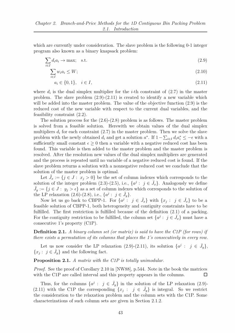
Chapter 2. Branch-and-Price Methods for the 1D Contiguous Bin Packing Problem2.1. Introduction
which are currently under consideration. The slave problem is the following 0-1 integerprogram also known as a binary knapsack problem:
∑
i∈I
diai → max; s.t. (2.9)
∑
i∈I
wiai ≤W ; (2.10)
ai ∈ {0, 1}, i ∈ I, (2.11)
where di is the dual simplex multiplier for the i-th constraint of (2.7) in the masterproblem. The slave problem (2.9)-(2.11) is created to identify a new variable whichwill be added into the master problem. The value of the objective function (2.9) is thereduced cost of the new variable with respect to the current dual variables, and thefeasibility constraint (2.2).
The solution process for the (2.6)-(2.8) problem is as follows. The master problemis solved from a feasible solution. Herewith we obtain values of the dual simplexmultipliers di for each constraint (2.7) in the master problem. Then we solve the slaveproblem with the newly obtained di and get a solution a∗. If 1−
∑i∈I dia
∗i ≤ −ǫ with a
sufficiently small constant ǫ ≥ 0 then a variable with a negative reduced cost has beenfound. This variable is then added to the master problem and the master problem isresolved. After the resolution new values of the dual simplex multipliers are generatedand the process is repeated until no variable of a negative reduced cost is found. If theslave problem returns a solution with a nonnegative reduced cost we conclude that thesolution of the master problem is optimal.
Let Jx := {j ∈ J : xj > 0} be the set of column indexes which corresponds to thesolution of the integer problem (2.3)-(2.5), i.e., {aj : j ∈ Jx}. Analogously we defineJy := {j ∈ J : yj > ǫ} as a set of column indexes which corresponds to the solution ofthe LP relaxation (2.6)-(2.8), i.e., {aj : j ∈ Jy}.
Now let us go back to CBPP-1. For {aj : j ∈ Jx} with {xj : j ∈ Jx} to be afeasible solution of CBPP-1, both heterogeneity and contiguity constraints have to befulfilled. The first restriction is fulfilled because of the definition (2.1) of a packing.For the contiguity restriction to be fulfilled, the column set {aj : j ∈ Jx} must have aconsecutive 1’s property (C1P).
Definition 2.1. A binary column set (or matrix) is said to have the C1P (for rows) ifthere exists a permutation of its columns that places the 1’s consecutively in every row.
Let us now consider the LP relaxation (2.9)-(2.11), its solution {aj : j ∈ Jy},{xj : j ∈ Jy} and the following fact.
Proposition 2.1. A matrix with the C1P is totally unimodular.
Proof. See the proof of Corollary 2.10 in [NW88], p.544. Note in the book the matriceswith the C1P are called interval and this property appears in the columns.
Thus, for the columns {aj : j ∈ Jy} in the solution of the LP relaxation (2.9)-(2.11) with the C1P the corresponding {xj : j ∈ Jy} is integral. So we restrictthe consideration to the relaxation problem and the column sets with the C1P. Somecharacterizations of such column sets are given in Section 2.1.2.
43

Chapter 2. Branch-and-Price Methods for the 1D Contiguous Bin Packing Problem2.1. Introduction
2.1.2 Column sets and bipartite graphs
Let C := {cj ∈ {0, 1}m : j ∈ JC} be a column set for an JC := {1, . . . , n}. Thebipartite graph BC := (V C
1 , VC
2 , EC) associated to the column set C is defined byV C
1 := I, V C2 := JC , and EC := {(i, j) ∈ V C
1 × V C2 : cj
i = 1}, see Fig. 2.1. Abipartite graph is convex if its half adjacency matrix1 has the C1P. For the column seton Fig. 2.1a the corresponding bipartite graph, see Fig. 2.1b, is non-convex.
Let (p→ q) for p, q ∈ V C2 be the set of vertexes from V C
1 ∪VC
2 , which are in a pathfrom p to q. Hence, if there does not exist a path from p to q with p, q ∈ V C
2 in BC
then (p→ q) = ∅.Let N(k) := {i ∈ V C
1 : cki = 1} be the closed neighborhood of a node k ∈ V C
2 , seeFig. 2.1.
A B C D
a 1 1 0 1b 0 1 1 0c 0 0 1 1d 0 0 0 0e 0 1 1 1
(a)
a
b
c
d
e
A
B
C
D
(b)
Figure 2.1: Column set without the C1P: (a) – A column set; (b) – The correspondingbipartite graph. The property is broken in the subcolumns of the columns B, C, Dwhich are marked by the dashed box. Thus, the corresponding bipartite graph is non-convex. The closed neighborhoods of each vertex is N(A) := {a}, N(B) := {a, b, e},N(C) := {b, c, e}, and N(D) := {a, c, e}. The bipartite graph has a single asteroidaltriple, namely (B,C,D) because only for these vertexes there exist the paths (B →C)D := {B, b, C}, (C → D)B := {C, c,D}, and (B → D)C := {B, c,D}.
A characterization of the graphs corresponding to the column sets with the C1Pwas given by A. Tucker. The characterization in given in terms of so-called asteroidaltriples (A-triples) [Tuc72] defined as follows.
Definition 2.2. Let BC := (V C1 , V
C2 , EC) be a bipartite graph. Vertexes p, q, r ∈ V C
2
with p 6= q, q 6= r, and p 6= r form an A-triple, if (p → q) 6= ∅, (p → r) 6= ∅,(q → r) 6= ∅, and:
(p→ q) ∩N(r) = ∅ ∧ (p→ r) ∩N(q) = ∅ ∧ (q → r) ∩N(p) = ∅.
On Fig. 2.1b there is only one A-triple, namely (B,C,D). Note in [Tuc72] a commongraph is considered not the bipartite one. We deal with bipartite graphs, so we defineA-triples only for them.
Let (p → q)r be a path from p to q without the closed neighborhood of r: (p →q)r ∩N(r) = ∅.
The following theorem characterizes convex bipartite graphs.
1We deal with undirected bipartite graphs, therefore only one part of the adjacency matrix isenough to define the corresponding graph.
44

Chapter 2. Branch-and-Price Methods for the 1D Contiguous Bin Packing Problem2.1. Introduction
Theorem 2.2 ([Tuc72, Theorem 6, p.156]). Let BC := (V C1 , V
C2 , EC) be the bipartite
graph associated to a column set C. The set C has the C1P if and only if V C2 contains
no A-triple of BC .
The roles of V1 and V2 are interchanged here compared to [Tuc72]. A direct consequenceof Theorem 2.2 are the following corollaries.
Corollary 2.3. A column set C := {cj ∈ {0, 1}m : j ∈ JC} has the C1P if and onlyif the associated bipartite graph BC := (V C
1 , VC
2 , EC) with V C1 := I, V C
2 := JC containsno A-triple.
Corollary 2.4. A column set C := {cj ∈ {0, 1}m : j ∈ JC} does not have the C1P ifand only if the associated bipartite graph BC := (V C
1 , VC
2 , EC) with V C1 := I, V C
2 := JC
contains at least one A-triple.
Another Tucker’s characterization of graphs having no A-triple is given in the fol-lowing theorem.
Theorem 2.5 ([Tuc72, Theorem 7, p.157]). In a bipartite graph BC := (V C1 , V
C2 , EC)
the vertex set V C2 contains no A-triple if and only if BC contains none of the graphs
G1k, G2
k, G3k (with k ≥ 1), G4, and G5 as shown in Fig. 2.2.
A direct consequence of Theorem 2.5 is the following corollary.
Corollary 2.6. A bipartite graph BC := (V C1 , V
C2 , EC) has at least one A-triple if and
only if BC contains one or more graphs G1k, G2
k, G3k, G4, and G5 as a subgraph.
2.1.3 Overview of solution methods
A position-indexed formulation for CBPP-1 is considered in [HNS08] where a branch-and-cut algorithm based on some facet-defining inequalities is proposed. However,the proposed model has different drawbacks, the most crucial of which is the pseudo-polynomial number of position-indexed variables.
In [MMBS11], CBPP-1 is handled by branch-and-bound methods with the lowerbounds based on the LP relaxation of the Dantzig-Wolfe decomposed of the 1D binpacking problem which is solved by the column generation method. The approachwith the decomposed model is similar to those which are considered in this paper. Themain difference is that here we propose branch-and-price algorithms in contrast to thecombinatorial enumeration algorithms in [MMBS11]. Here we also tighten the columngeneration.
2.1.4 Our contribution
In order to solve CBPP-1 we use a Gilmore-Gomory model for the 1D bin packingproblem which was discussed in Section 2.1. In this section we use the know fact thatif a column set has the C1P then the corresponding matrix is total unimodular andthus all the corners of the polyhedron of its LP relaxation are integer for the integer
45

Chapter 2. Branch-and-Price Methods for the 1D Contiguous Bin Packing Problem2.2. The branch-and-price algorithms
...
k
(a) G1k
ω
µ
υ
a
b
...
k + 1
(b) G2k
ω
µ
υa
...
k + 1
(c) G3k
υ
µ
ω
(d) G4
υ
A
Bω
µ
ab
c
d
(e) G5
Figure 2.2: Forbidden subgraphs. The vertex set V C2 of a bipartite graph BC :=
(V C1 , V
C2 , EC) contains an A-triple if and only if BC contains one of the displayed
graphs as an induced subgraph where black vertexes correspond to vertexes in V C2 .
Numbers k and k+ 1 refer to the numbers of white vertexes in the right-hand parts ofthe first three graphs. In the case of the graph G1
k, any three different black vertexesbuild an A-triple. In other cases there is only a single A-triple, namely (υ, µ, ω).
input data. For the construction of such column sets, in Section 2.2 we develop branch-and-price algorithms with two strategies: column-, and subcolumn-based enumerations.In Sections 2.3, 2.4 we prove propositions about some characteristics of a specific oran arbitrary column which breaks the C1P of a given column set. For each of thesecharacteristics we develop an algorithm the output data of which is used in the slaveproblem of the column generation thus tightening the bound. The final part of thepaper reports numerical results and conclusion.
2.2 The branch-and-price algorithms
Here we describe the overall algorithm of finding an optimum of CBPP-1. The algo-rithm is a hybrid of the branch-and-bound and the column generation methods, i.e.,throughout the branching tree the column generation is applied for solving the LPrelaxation. The idea is the same as in branch-and-bound, we calculate lower boundsfor each node and use it as a pruning criteria.
In practice, for the branching-and-price, we store the columns which we generatethroughout the optimization process in a column pool. Processing from one node tothe descendants is done by adding a box-constraint for the corresponding variable. Sostoring the column indexes for each node is enough to reconstruct the formulation.
46

Chapter 2. Branch-and-Price Methods for the 1D Contiguous Bin Packing Problem2.2. The branch-and-price algorithms
As we have shown in Section 2.1.1, the solution of the LP relaxation (2.9)-(2.11)with the C1P is integral. Thus, our goal now is to enumerate column sets with theC1P.
The idea of branchings consist in an enumeration of feasible 1D partial packingshaving the C1P. On each step all columns with indexes J+ ⊆ J , i.e., {aj : j ∈ J+},are fixed to appear in the packing while all columns with indexes J− ⊆ J must notappear, i.e., {aj : j ∈ J−}. The column set {aj : j ∈ J+} is constructed such thatthe C1P arise.
Let V be the set of nodes of the branching tree T := (V,E), which are connectedby the edges from the set E. Hereby the sets J+(u) and J−(u) are associated witheach node u ∈ V .
Given a node u ∈ V of the branching tree and having the sets J+(u) and J−(u)in mind, the master problem of the column-generation method becomes the followingform:
LP(u) : φ(u) =∑
j∈J
yj → min; s.t. (2.12)
∑
j∈J
ajiyj = hi, i ∈ I; (2.13)
yj ≥ 1, j ∈ J+(u); (2.14)
yj = 0, j ∈ J−(u); (2.15)
yj ≥ 0, j ∈ (J \ J+(u)) \ J−(u), (2.16)
and the slave problem:
CG(u) :∑
i∈I
diai → max; s.t. (2.17)
∑
i∈I
wiai ≤W ; (2.18)
∑
i∈I
[ai(1− aji ) + aj
i (1− ai)] > 0, j ∈ J−(u); (2.19)
ai ∈ {0, 1}, i ∈ I. (2.20)
where the constraints (2.19) exclude the solutions from J−(u) from the feasible set ofsolutions.
Let J(u) := {j ∈ J : yj > ǫ} be the set of column indexes which are in the solutionof LP(u). Some of the columns {aj : j ∈ J(u)} build together with the columnswith indexes from J+(u) a column set having the C1P. Let J+(u) ⊆ J(u) be such that∀j ∈ J+(u), J+(u)∪{aj} has the C1P, and J−(u) := J(u)\ J+(u). For testing whethera column set has the C1P we use the PQ-tree algorithm [BL76].
In the following we introduce two branch-and-price algorithms which are distin-guished by the branching strategies.
2.2.1 A column-based branching strategy
Here we introduce a column-based branching strategy. The main idea is to constructthe solution having the C1P from the columns of the LP relaxation.
47

Chapter 2. Branch-and-Price Methods for the 1D Contiguous Bin Packing Problem2.2. The branch-and-price algorithms
Having the J+(u) and J−(u) sets we solve the LP relaxation and test the columnswhether they build with the columns {aj : j ∈ J+(u)} a column set with the C1P. Ifthere exists one then we branch on this column. If it does not exist then we tightenthe formulation of the LP relaxation and resolve until a column to branch is found, thenode is pruned considering the bound or it is proven that no column to branch exists.
Algorithm 2.1 (Branch-and-price-cols). A branch-and-price algorithm with thecolumn-based branching strategy.Input data: W , m, w = (w1, . . . , wm), h = (h1, . . . , hm).Output data: optimal solution (A, Y ) and its value H.
(1 ) Initialization:
• node u0, J+(u0) = J−(u0) := ∅.
• incumbent A := ∅, Y := ∅, H :=∞.
• node list N := {u0}.
(2 ) Node: If N = ∅, go to Exit. Else choose u ∈ N , set N := N\{u} and go toRestore.
(3 ) Restore the sets J+(u) and J−(u).(4 ) LP relaxation: Solve LP(u) considering J+(u) and J−(u) and obtain the solution
and hence the set J(u). For all j ∈ J(u) \ J+(u) test by the PQ-tree algorithm,if J+(u) ∪ {aj} has the C1P. If yes then set J+(u) := J+(u) ∪ {j}, else setJ−(u) := J−(u) ∪ {j}.
(5 ) Prune: If φ(u) ≥ H, go to Node. If the solution {yj : j ∈ J(u)} is integralthen set H := φ(u), update the incumbent (A, Y ) with A := {aj : j ∈ J(u)},Y := {yj : j ∈ J(u)} and go to Node, else go to Branching.
(6 ) Branching: Having J+(u) and J+(u) do:
(6.1 ) If J+(u) \ J+(u) = ∅ then create one node v with:
• J+(v) := J+(u).
• J−(v) := J−(u) ∪ J−(u).
Set N := N ∪ {v}. Go to Node.(6.2 ) If J+(u) \ J+(u) 6= ∅ then set j∗ := argmax{yj : j ∈ J+(u) \ J+(u)},
and create node v1:
• J+(v1) := J+(u) ∪ {j∗},
• J−(v1) := J−(u) ∪ J−(u),
and create node v2:
• J+(v2) := J+(u),
• J−(v2) := J−(u) ∪ J−(u) ∪ {j∗}.
Set N := N ∪ {v1, v2}. Go to Node.
(7 ) Exit: Return the incumbent (A, Y ) and its value H.
As we can see the main drawback of the described strategy is that we may createa lot of descendants while J+(u) \ J+(u) = ∅, see step 6.1 in Algorithm 2.1. For
48

Chapter 2. Branch-and-Price Methods for the 1D Contiguous Bin Packing Problem2.2. The branch-and-price algorithms
eliminating this drawback we tighten the column generation by forbidding not only thecolumns but subcolumns.
Let us consider the column set on Fig. 2.1 where four columns A, . . . , D, and fiverows a, . . . , e exist. Columns A, B, C together have the C1P. If we join them with thecolumn D then the obtained column set will not have the C1P. The property is brokennot in the whole matrix, but only in the part marked by the dashed box. Note if thereis a such combination a = 1, b = 0, c = 1 of rows in a column D, the C1P would notarise despite the values of d and e. So, if we now consider only columns were there isno such a combination of rows, we reduce the columns which break a priori the C1P.
Let a subcolumn dk be given by an index set Ik ⊂ I and coefficients dki , i ∈ Ik. For
a given node u ∈ V of the branching tree we consider a set of subcolumns D(u) :={dk : k ∈ K(u)} which breaks the C1P of the column set {aj : j ∈ J+(u)}. Hereby,if for some j ∈ J and k ∈ K(u): aj
i = dki , ∀i ∈ Ik then yj = 0 has to follow which is
realized in the master problem of the column generation by:
∑
i∈Ik
|aji − d
ki | = 0 ⇒ yj = 0, j ∈ (J\J+(u))\J−(u), k ∈ K(u).
The above constraint is nonlinear. For its tackling we remove it from the master prob-lem and add it to the slave problem CG(u) of the column generation in the followingform:
∑
i∈Ik
[ai(1− dki ) + dk
i (1− ai)] > 0, k ∈ K(u), (2.21)
which is herewith tightened.For construction of subcolumns for a given set of columns having the C1P we
propose two approaches. Suppose for a given u ∈ V we have J+(u) and the columnset {aj : j ∈ J+(u)}. The first approach uses the latter columns having the C1Pand construct the subcolumns which can potentially break the C1P. This approach isconsidered in Section 2.4.
Based on u, J+(u) and due to Algorithm 2.1, we solve LP(u) and obtain the setJ(u). Afterward we apply the PQ-tree algorithm for each j ∈ J(u) \ J+(u) and defineJ−(u). Now from the columns {aj : j ∈ J−(u)} we find the subcolumns which breakthe C1P. This is the second approach which is considered in Section 2.3.
2.2.2 A subcolumn-based branching strategy
Here we introduce a subcolumn-based branching strategy. This branching strategy wasfirstly discussed in [Bel10]. The main idea of the branching strategy is to branch on thesubcolumns which break the C1P of the current basis solution of the LP relaxation.
Having a basis solution of the LP relaxation we test it for the C1P by the PQ-tree algorithm [BL76]. If it does not have the C1P then the basis solution containedone or more submatrices of the types MI , . . . ,MV in [Tuc72], Fig. 3, p.161. Note thecorresponding matrix will contain one or more of the graphs from Fig. 2.2 as a subgraph.The submatrices of the types MI , . . . ,MV can be found by the algorithms described in[Dom09], Chapter 3, p.63–78.
49

Chapter 2. Branch-and-Price Methods for the 1D Contiguous Bin Packing Problem2.3. Subcolumns breaking the C1P
Algorithm 2.2 (Branch-and-price-subcols). A branch-and-price algorithm withthe subcolumn-based branching strategy.Input data: W , m, w = (w1, . . . , wm), h = (h1, . . . , hm).Output data: optimal solution (A, Y ) and its value H.
(1 ) Initialization:
• node u0, D(u0) := ∅.
• incumbent A := ∅, Y := ∅, H :=∞.
• node list N := {u0}.
(2 ) Node: If N = ∅, go to Exit. Else choose u ∈ N , set N := N\{u} and go toRestore.
(3 ) Restore the set D(u).(4 ) LP relaxation: Let J(u) be the set of columns from the column pool and let
Jd(u) := {j ∈ J(u) : aji (1 − dk
i ) + dki (1 − aj
i ) = 0, dk ∈ D(u)} be the set ofindexes of columns from J(u) which contain a forbidden subcolumn from D(u).Solve the following LP relaxation considering D(u) and Jd(u):
LP’(u) : φ(u) =∑
j∈J
yj → min; s.t. (2.22)
∑
j∈J
ajiyj = hi, i ∈ I; (2.23)
yj = 0, j ∈ Jd(u); (2.24)
yj ≥ 0, j ∈ J \ Jd(u), (2.25)
and obtain the solution and hence the set J(u). By the PQ-tree algorithm testif {aj : j ∈ J(u)} has the C1P. If yes then goto Prune, else find a submatrixF (u) := {f1, . . . , fσ(u)} of the types MI , . . . ,MV in {aj : j ∈ J(u)}.
(5 ) Prune: If φ(u) ≥ H, go to Node. If the solution {yj : j ∈ J(u)} is integralthen set H := φ(u), update the incumbent (A, Y ) with A := {aj : j ∈ J(u)},Y := {yj : j ∈ J(u)} and go to Node, else go to Branching.
(6 ) Branching: Create nodes vk with k = 1, . . . , σ(u): D(vi) := D(u) ∪ {fk}, setN := N ∪ {vk}. Go to Node.
(7 ) Exit: Return the incumbent (A, Y ) and its value H.
2.3 Subcolumns breaking the C1P
Here we consider an approach of finding the subcolumns of a given column which breaksthe C1P of a given set of columns having the C1P.
Now going back to a node u ∈ V of the branching tree T we can conclude usingCorollary 2.3 that since {aj : j ∈ J+(u)} has the C1P then the corresponding bipartitegraph has no A-triple. The following statement is true.
50

Chapter 2. Branch-and-Price Methods for the 1D Contiguous Bin Packing Problem2.3. Subcolumns breaking the C1P
Statement 2.7. Let u ∈ V be a node of the branching tree T and let aγ with γ ∈J \ J+(u). The column set C := {aγ}∪{aj : j ∈ J+(u)} does not have the C1P if andonly if the associated bipartite graph BC := (I, {1, . . . , |C|}, EC) contains at least oneA-triple.
Remark 2.1. An A-triple which exists in BC may contain the vertex γ and may notcontain it as well.
Hereby, if we join the columns {aj : j ∈ J+(u)} with a column aj with j ∈J−(u), the resulting set will not have the C1P and according to Statement 2.7 thecorresponding bipartite graph will have at least one A-triple.
Let JC ⊆ J and C := {aj : j ∈ JC} be a set of columns and let C(Ir, Ic) :={aj
i : i ∈ Ir, j ∈ Ic} be the set of the columns from Ic ⊂ JC and the rows from Ir ⊂ I.The following lemma is true.
Lemma 2.8. If a column set C has the C1P then the set C(Ir, Ic) will also have theC1P for any Ir ⊂ I and Ic ⊂ JC.
Proof. Let us prove the lemma for elements k ∈ I\Ir and d ∈ JC\Ic. Let C be a sethaving the C1P. Due to Theorem 2.2, the corresponding bipartite graph BC has noA-triple. Let us consider the set C(I\{k}, JC\{d}) and assume that it does not havethe C1P. Due to Corollary 2.4, the corresponding bipartite graph BC(I\{k},JC\{d}) hasat least one A-triple, e.g., (υ, µ, ω) with υ 6= µ, µ 6= ω, and υ 6= ω. It means that{k, d} ∩ [(υ → µ)ω ∪ (υ → ω)µ ∪ (µ → ω)υ] = ∅, while (υ → µ)ω 6= ∅, (υ → ω)µ 6= ∅,and (µ → ω)υ 6= ∅. The latter follows that the paths (υ → µ)ω, (υ → ω)µ, (µ → ω)υ
must exist also in the graph BC . Hence, (υ, µ, ω) is an A-triple in BC and due toCorollary 2.4 the set C does not have the C1P which contradicts the condition that Chas the C1P. Hereby we set I := I\{k}, JC := JC\{d} and repeat the above procedureuntil I = Ir and JC = Ic.
Let d∗ be a subcolumn which breaks the C1P of {aj : j ∈ J+(u)} and be givenby an index set I∗ ⊂ I and coefficients d∗
i with i ∈ I∗. If C(I∗, JC) ∪ {d∗} does nothave the C1P then d∗ is called ineligible. An ineligible subcolumn is called minimal if∄i∗ ∈ I∗:
d∗ =
1− di, i = i∗,
di, i ∈ I∗\{i∗},
so that C(I∗, JC) ∪ {d∗} does not have the C1P.
Theorem 2.9. If d∗ is a minimal ineligible subcolumn then 1 ≤∑
i∈I∗d∗
i ≤ 3 is true.
Proof. Since C(I∗, JC) ∪ {d∗} does not have the C1P then due to Corollary 2.4 thecorresponding bipartite graph contains at least one A-triple. Therefore, due to Corol-lary 2.6 the bipartite graph contains one or more graphs G1
k, G2k, G3
k, G4, and G5 as asubgraph. Since d∗ corresponds to a vertex of the set V2, the number of 1’s in d∗ is adegree of the corresponding vertex which can be any of V2. Let us calculate minimaland maximal degrees of vertexes from V2 of G1
k, G2k, G3
k, G4, and G5, respectively.
51

Chapter 2. Branch-and-Price Methods for the 1D Contiguous Bin Packing Problem2.3. Subcolumns breaking the C1P
Let us consider the graph G1k. If we take any υ, µ, ω ∈ V
G1k
2 with υ 6= µ, υ 6= ω, andµ 6= ω then there would exist nonempty paths (υ → µ)ω, (υ → ω)µ, and (µ → ω)υ
which means that (υ, µ, ω) is an A-triple. Note if we delete one of the edges which
is incident to a vertex from VG1
k2 in the graph then one of the three paths would not
exist and hence no A-triple. So, the minimal and the maximal vertex degree for G1k
are equal to 2.
Let us consider the graph G2k. It has such a construction, so that there exists only
one A-triple, namely (υ, µ, ω). Moreover the path (µ → ω)υ must not contain thevertexes a and b due to the definition of A-triples. So the single path which satisfiesthis condition goes through the white and the black vertexes except υ, a, and b. Let d∗
correspond to a black vertex except υ, µ, and ω. The above described path containsnecessarily this vertex. Every such vertex has the degree equal to 4. Actually, if wedelete two edges which make this vertex incident to a and b then the path (µ → ω)υ
would still exist and the A-triple as well. It means that these two edges are excessiveand are not necessary to build the A-triple. It is also obvious that both of the twoedges which outcome from the vertexes υ, µ, and ω are necessary to build the A-triple.So, the minimal and the maximal vertex degree for G2
k are equal to 2 in order to buildthe A-triple (υ, µ, ω).
Let us consider the graph G3k. The A-triple is constructed only by the vertexes υ,
µ, and ω. We have the same path between µ and ω as in the case of G2k, the path goes
only through the white and the black vertexes except υ, and a. Let d∗ correspond toa black vertex except υ, µ, and ω. The edge which makes the vertex incident to a isactually excessive because the path (µ→ ω)υ does not contain the vertex a. But theremust be at least one black vertex which is incident to a for the existence of the paths(υ → µ)ω and (υ → ω)µ. It is also obvious that the edge outcomming from υ, µ, and ωis necessary to build the A-triple. So, the vertex degree for G3
k lies in the interval from1 to 3 in order to build the A-triple (υ, µ, ω).
Let us consider the graph G4. It obvious that the deletion of an edge in the graphG4 will break the coherence of the graph G4 which leads to the graph with no A-triple.So, the vertex degree for G4 lies in the interval from 1 to 2 in order to build the A-triple(υ, µ, ω).
Let us consider the graph G5. The vertexes υ, µ, and ω create the single A-triple,so that the paths (υ → µ)ω, (υ → ω)µ, and (µ→ ω)υ are not empty. Let d∗ correspondto µ or ω. In this case the edges (µ, b) and (ω, b) are excessive because the abovedescribed paths are not empty without these edges, i.e., (υ → µ)ω = {υ,A, c, µ},(υ → ω)µ = {υ,B, d, ω}, and (µ → ω)υ = {µ, c, A, b, B, d, ω}, so the one outcommingegde (µ, c) and (ω, d) for µ and ω is sufficient. Let d∗ correspond to A or B. Then theedges (b, B), and (b, A) are excessive for the same reason, i.e., (υ → µ)ω and (υ → ω)µ
are the same, but (µ → ω)υ = {µ, b, ω}. It is also obvious that there must exist theedge (υ, a). Therefore, the vertex degree for G5 lies in the interval from 1 to 2 in orderto build the A-triple (υ, µ, ω).
The above implies the validity of 1 ≤∑
i∈I∗d∗
i ≤ 3.
Lemma 2.10. If∑
i∈I∗d∗
i = 1 then the vertex corresponding to d∗ is contained in oneof the A-triples.
52

Chapter 2. Branch-and-Price Methods for the 1D Contiguous Bin Packing Problem2.3. Subcolumns breaking the C1P
Proof. Since C(I∗, JC) ∪ {d∗} does not have the C1P then due to Corollary 2.4 thecorresponding bipartite graph contains at least one A-triple. Therefore, due to Corol-lary 2.6 the bipartite graph contains one or more graphs G1
k, G2k, G3
k, G4, and G5 asa subgraph. Since
∑i∈I∗
d∗ = 1 is minimal then the corresponding vertex is terminal.In the above described graph all terminal vertexes correspond to the vertexes of theA-triple.
Theorem 2.11. If a subcolumn d∗ is minimal then the corresponding bipartite graphcontain one of the graphs G1
k, G2, G3, and G4.
...
k
(a) G1k
υ
µ
ω
(b) G2
υ
µ
ω
(c) G3
υ
A
Bω
µ
ab
c
d
(d) G4
Figure 2.3: Forbidden subgraphs G1k, G
2, G4, G4.
Proof. Since C(I∗, JC) ∪ {d∗} does not have the C1P then due to Corollary 2.4 thecorresponding bipartite graph contains at least one A-triple. Therefore, due to Corol-lary 2.6 the bipartite graph contains one or more graphs G1
k, G2k, G3
k, G4 and G5 as asubgraph.
Let us consider the situation before we add the vertex corresponding to d∗ to thebipartite graph. In the case of G1
k the graph lacks one of the black vertexes. It isobvious that connecting of two white vertexes with the vertex degree equal to 1 withthe new vertex will create an A-triple. Moreover, this is the single connection with theminimal number of edges in order to get an A-triple. Other connections will containthe mentioned edges. The same is with the graph G4, see Fig. 2.3c.
Let us consider the graphs G2k and G3
k. There exist only a single A-triple (υ, µ, ω). Itmeans that there exist the paths (µ→ ω)υ, (υ → µ)ω, and (υ → ω)µ. The second andthe third paths do not contain the edges (b, ω) and (a, µ), and the first path goes onlythrough the right-hand white vertexes. So, the edges (b, ω) and (a, µ) can be removed.Hence the graphs G2
k and G3k are equivalent in the sense of the mentioned paths. So,
let us consider the graph G3k before we add the vertex corresponding to d∗. The cases
where the graph lacks υ, µ, and ω are obvious. In other case it is enough to add theedges starting from the white vertexes with the degree equal to 1, see the graph G2
in Fig. 2.3b. All other possible constructions building an A-triple will contain theseedges.
Let us consider the graph G5. There exists a single A-triple (υ, µ, ω) with the twodifferent existing paths, see Fig. 2.4. It is obvious that the path (a,B, d, ω) in thegraph G5′
is excessive, so that the graph is equivalent to the graph G2. Let us consider
53

Chapter 2. Branch-and-Price Methods for the 1D Contiguous Bin Packing Problem2.3. Subcolumns breaking the C1P
υ
A
Bω
µ
ab
c
d
(a) G5′
υ
A
Bω
µ
ab
c
d
(b) G5′′
Figure 2.4: Forbidden subgraph G5: different paths.
the graph G5′′
and the situation before we add the vertex corresponding to d∗. In thecase where υ do not exist, any three vertexes of {A,B, µ, ω} can build an A-triple.That contradicts the assumption that before we add a vertex to the graph it containsno A-triple. So, υ should be in the graph. In the case of µ or ω there exist only onepossibility to build an A-triple, namely to add the edges (µ, c), (µ, b) or (ω, d), (ω, b),respectively. In the case of the vertex A, there exist two possibilities. The first one isto add the edge (A, d), so that an A-triple as in G1
k arises. The second one is to addthe edge (A, a). The same is with the vertex B.
Lemma 2.12. Let d∗ be a minimal ineligible subcolumn. If there exists an A-triplecontaining the vertex corresponding to d∗ then 1 ≤
∑i∈I∗
d∗i ≤ 2 is true.
For the proof refer to the next lemma.
Lemma 2.13. If d∗ is a minimal ineligible subcolumn then 1 ≤∑
i∈I∗d∗
i ≤ 3 is true.
Proof. Before we add a vertex to the graph the latter does not contain any A-triples.Since we add the vertex corresponding to the minimal d∗ then due to Theorem 2.11there arise one or more graphs G1
k, G2, G3, and G4. Both Lemmas 2.12 2.13 are easyto prove considering the above mentioned graphs. Correctness of Lemma 2.12 followsfrom the fact that the maximal degree of the black vertexes which are contained inan A-triple is equal to 2. Correctness of Lemma 2.13 follows from the fact that themaximal degree of a black vertex in all graphs is equal to 3, see Fig. 2.3b.
Let us go back to the column aγ with γ ∈ J−(u) and the subcolumn dk witha minimal size. As noted in Remark 2.1 there exist two possibilities of how an A-triple arise due to Statement 2.7 in the bipartite graph corresponding to {aj : j ∈J+(u)} ∪ {aγ}. In the first one, the obtained A-triple contains γ. In the other one,the obtained A-triple contains only vertexes from V C
2 with C := {aj : j ∈ J+(u)}where aγ serves only as a connection for the arising paths. In the first case, e.g., whenthe terms of Lemma 2.10 are satisfied, it is enough to find A-triples which starts withγ. For that purpose we use the characterization given in Lamma 2.12. This case isconsidered further in Algorithm 2.3. In the second case we apply Algorithm 2.4 whichuses the characterization given in Lemma 2.13.
54

Chapter 2. Branch-and-Price Methods for the 1D Contiguous Bin Packing Problem2.3. Subcolumns breaking the C1P
Let us consider the case where A-triples contain γ. Based on a set C := {aj : j ∈J+(u)} we build the corresponding convex bipartite graph Bγ without vertexes andedges which could be incident to γ, if we would add it to V C
2 . The resulting columnset has the C1P due to Lemma 2.8 and the corresponding graph Bγ has no A-triplesdue to Corollary 2.3.
We search for all shortest paths between all two different vertexes of V γ2 in Bγ, refer
to Algorithm 2.3. Those pairs of vertexes for which there exist a path we consideras candidates entering to an A-triple together with the vertex γ due to Statement 2.7and the assumption that the obtained A-triple contains γ. Now we test whether thereexists a path between vertexes of these pairs and γ every time avoiding the closedneighborhood of the third vertex, respectively. If all three paths exist then (γ, p, q)builds an A-triple. All vertexes from I which are in these paths correspond to thedesired subcolumn.
Algorithm 2.3 (Subcol-of-a-col-A). Determination of forbidden subcolumns of agiven column in the case when A-triples start with the vertex corresponding to the givencolumn.Input data: A node u, the column aγ with γ ∈ J−(u).Output data: D(u).
(1 ) For each pair of vertexes p, q ∈ V2 with p < q find a shortest path (p → q) fromp to q in
Bγ := (V γ1 := I\N(γ), V γ
2 := J+(u), Eγ := {(i, j) ∈ V γ1 × V
γ2 : aj
i = 1}).
If (p→ q) 6= ∅ then add (p, q) to P0.(2 ) For each p, q ∈ V2 with p < q find a shortest path from γ to q without nodes in
the closed neighborhood of p, i.e., find (γ → q)p in
Bp := (V p1 := I\N(p), V p
2 := J+(u)∪{γ}\{p}, Ep := {(i, j) ∈ V p1 ×V
p2 : aj
i = 1}).
If (γ → q)p 6= ∅ then add (γ, q) to Pp.(3 ) For each (p, q) ∈ P0:
If (γ, p) ∈ Pq and (γ, q) ∈ Pp then (γ, p, q) forms an A-triple, hence forma subcolumn d∗ of aγ:d∗
i = aγi , ∀i ∈ Ik with Ik := [(p→ q) ∪ (γ → q)p ∪ (γ → p)q] ∩ I,
add d∗ to D(u), if d∗ /∈ D(u).
Lemma 2.14. Let u ∈ V be a node of the branching tree T , and aγ with γ ∈ J−(u).The algorithm Subcol-of-a-col-A is correct and returns in O(m2(M + logm)) timea subcolumn of aγ which breaks the C1P, if in the corresponding bipartite graph thereexists any A-triple containing γ.
Proof. The proof of the lemma consists of two parts. Let C+u := {aj : j ∈ J+(u)} and
C := C+u ∪{a
γ}. Since C does not have the C1P and due to Statement 2.7 there existsan A-triple, we should prove that the algorithm finds this A-triple. Secondly, the timecomplexity should be calculated.
55

Chapter 2. Branch-and-Price Methods for the 1D Contiguous Bin Packing Problem2.3. Subcolumns breaking the C1P
So, due to Corollary 2.6, the graph BC
:= (V C1 , V
C2 , EC
) has at least one of thegraphs G1
k, G2k, G3
k, G4, and G5 as a subgraph. Let G1k be such a graph. Due to
Corollary 2.3, the bipartite graph BC+u
has no A-triple. Since the sets V C2 and V C+
u2
differ only in one element, namely γ, it means that γ builds an A-triple together with
two other vertexes p, q with p 6= q from V C+u
2 which are in the vertex set of G1k. Note
there always exists a path (p → q) in BC+u
which is found on step 1 of the algorithm.Fig. 2.2a indicates also that there exist the paths (γ → p)q and (γ → q)p which arefound on step 2 of the algorithm. Since all three paths (p→ q), (γ → p)q, and (γ → q)p
exist then (γ, p, q) is found on step 3 of the algorithm. The same can be proved for G2k,
G3k, G4, and G5, see Fig. 2.2.
The time complexity is calculated as follows. It performs m2 operations to con-struct a bipartite graph using a matrix. So, graph Bγ is build in O(m2) time (step 1).The rest can be done by one run of the Dijkstra’s algorithm or the Floyd-Warshall’salgorithm (WFI) [CLR90]. The complexity of the Dijkstra’s algorithm is O(|EC | +(|V1 + V2|) log(|V1 + V2|)) where |EC | is the number of edges and |V1 + V2| = 2mis the number of vertexes in the graph. Concerning that the maximal number ofitems fitting into a bin is M := max{
∑i∈I ai :
∑i∈I wiai ≤ W, ai ∈ {0, 1}}, so
the number of 1’s in the whole matrix, thus number of edges is |E| = mM . Hence,O(|EC|+ (|V1 + V2|) log(|V1 + V2|)) = O(mM + 2m log 2m) and the complexity of step1 is O(m2(M + logm)). Therefore, the complexity of step 2 is also the same becausethe graph Bp can be obtained by a linear modification of Bγ . Since the cardinalityof the set P0 is m
2(m − 1), and we need a constant time to test whether a path is in
Pp (step 3), the complexity of this step is O(m2). Therefore, Subcol-of-a-col-A’scomplexity is O(m2(M + logm)).
Remark 2.2. M in the formula of Subcol-of-a-col-A’s complexity tends to beconstant, but large. Hence, Subcol-of-a-col-A’s complexity is O(m2 logm).
Let us consider the case, where A-triples do not contain γ. Based on C := C+u ∪{a
γ}
we build bipartite graph B = (V C1 , V
C2 , EC
), which due to Statement 2.7 contains anA-triple. In order to find this A-triple we compute all shortest paths between two
different vertexes p and q not equal to γ from V C2 in BC each time avoiding the direct
neighborhood of the third vertex r. Herewith, we obtain the set Prpq for all p, q and r.
Due to the assumption the obtained A-triple does not contain γ, so for all different p,q, r and not equal to γ we test whether paths (p → q)r ∈ Pr
pq, (p → r)q ∈ Pqpr, and
(q → r)p ∈ Ppqr. If so then p, q, and r build an A-triple. Algorithm 2.4 contains details
of the above algorithm.
Algorithm 2.4 (Subcol-of-a-col-B). Determination of forbidden subcolumns of agiven column in the case when A-triples do not contain γ.Input data: A node u, the column aγ with γ ∈ J−(u).Output data: D(u).
(1 ) For each vertex p, q, r ∈ J+(u) with p < q, r 6= p and r 6= q, find a shortest path(p→ q)r from p to q without the closed neighborhood of γ in
Br := (V r1 := I\N(r), V r
2 := (J+(u)\{r})∪{γ}, Er := {(i, j) ∈ V r1 ×V
r2 : aj
i = 1}).
56

Chapter 2. Branch-and-Price Methods for the 1D Contiguous Bin Packing Problem2.4. Subcolumns potentially breaking the C1P
If (p→ q)r 6= ∅ then add (p, q)r to Prpq.
(2 ) For each p, q, r ∈ J+(u) with p 6= q, q 6= r, and p 6= r:If (p, q)r ∈ Pr
pq and (q, r)p ∈ Ppqr and (p, r)q ∈ Pq
pr then (p, q, r) forms anA-triple, hence form the subcolumn d∗ of aγ:d∗
i = aγi , ∀i ∈ Ik with
Ik := [N(γ) ∩ (p→ q)r] ∪ [N(γ) ∩ (p→ r)q] ∪ [N(γ) ∩ (q → r)p],add d∗ to D(u), if d∗ /∈ D(u).
Lemma 2.15. Let u ∈ V be a node of the branching tree T , and aγ with γ ∈ J−(u).The algorithm Subcol-of-a-col-B is correct and returns in O(m3(M + logm)) timea subcolumn of aγ which breaks the C1P, if in the corresponding bipartite graph thereexists any A-triple which does not contain γ.
Proof. The time complexity can be calculated as follows. It performs m2 operationsto construct a bipartite graph using a matrix. So, the graph Br is build in O(m2)time (step 1). The rest can be done by one run of the Dijkstra’s algorithm or theFloyd-Warshall’s algorithm (WFI) [CLR90]. As it was shown, it takes O(|EC |+ (|V1 +V2|) log(|V1 + V2|)) = O(mM + 2m log 2m) operations, so the total complexity of step1 is O(m3(M + logm)). Since the test whether (p, q)r ∈ Pr
pq for any p, q, r is constant,and we perform this test for each p, q, and r then the complexity of step 2 is O(m3).Therefore, Subcol-of-a-col-B’s complexity is O(m3(M+logm)+m3) = O(m3(M+logm)).
Remark 2.3. M in the formula of Subcol-of-a-col-B’s complexity tends to beconstant, but large. Hence, Subcol-of-a-col-B’s complexity is O(m3 logm).
2.4 Subcolumns potentially breaking the C1P
Let u ∈ V be a node of the branching tree T . Let us now answer the following question:what combinations of elements of a column will break the C1P of C+
u := {aj : j ∈J+(u)} being joint with a column? In order to solve this problem we perform thefollowing steps. Firstly, we use the associated bipartite graph B0 := (V1, V2, E0) basedon C+
u and search for every vertex all vertex-disjoint paths to any other vertex. GraphB0 has no A-triples due to Corollary 2.3.
Definition 2.3. Let (p → q)1 := {t11, . . . , t1l }, . . . , (p → q)χ := {tχ1 , . . . , t
χl } be paths
from p to q with (p → q)1 = . . . = (p → q)χ. Path (p → q)φ with φ ∈ {1, . . . , χ} isexclusive if tφj ≤ tfj , f ∈ {1, . . . , χ}\{φ}, j = 1, . . . , l.
So, only exclusive paths are considered.Let us consider an imaginary column sγ ∈ {0, 1}m represented by a vertex γ when
added to B0. γ is incident to every vertex of V1. We suppose that now γ induces anA-triple together with the vertexes from V2. Due to Statement 2.7 the set C+
u ∪ {sγ}
does not have the C1P. Now for every initial and final vertex p, q of the above pathswe determine whether there exist paths (γ → p) and (γ → q) each time avoiding adirect vertex and edge neighbors of q and p, respectively, and avoiding vertexes from
57

Chapter 2. Branch-and-Price Methods for the 1D Contiguous Bin Packing Problem2.4. Subcolumns potentially breaking the C1P
V1, which are in the path (p → q). If all three paths exist then (γ, p, q) is an A-triple.In such a way all A-triples are searched which can result when an additional columnis added to C+
u .Now going back to subcolumns we can conclude that items from V1 which were in
the paths (γ → p)q, (γ → q)p, and (p→ q) should correspond to the desired subcolumn.Moreover, the vertexes from V1 which are in (p → q) correspond to rows with 0 andvertexes which are in (γ → p)q, (γ → q)p and not in (p → q) correspond to rows with1 in the subcolumn. Algorithm 2.5 contains details of the above algorithm.
Algorithm 2.5 (Subcols). Determination of forbidden subcolumns.Input data: A node u, the column set {aj : j ∈ J+(u)}.Output data: D(u).
(1 ) Set B0 := (V1 := I, V2 := J+(u), E0 := {(i, j) ∈ V1 × V2 : aji = 1}).
(1.1 ) For each pair of vertexes p, q ∈ V2 with p < q find all exclusive paths from pto q, i.e., (p → q) in B0. So, we obtain the set Ppq of paths from p to q inB0.
(1.2 ) If two paths (p→ q)1 ∈ Ppq, (p→ q)2 ∈ Ppq satisfy V1(p→ q)1 & V1(p→ q)2
then delete (p→ q)2 from Ppq (where V1(p→ q) = {i ∈ V1 : i ∈ (p→ q)}).
(2 ) Set Bp := (V p1 := I\N(p), V p
2 := V2\{p}, Ep := {(i, j) ∈ V p1 × V
p2 : aj
i = 1}).
(2.1 ) For all p ∈ V2 and all i /∈ N(p) find for all q ∈ V2\{p} all exclusive pathsfrom i to q in Bp. So, we obtain set Pp
iq of paths from i to q without theclosed neighborhood of vertex p in Bp.
(2.2 ) If two paths (i→ q)p1 ∈ P
piq, (i→ q)p
2 ∈ Ppiq satisfy V1(i→ q)p
1 & V1(i→ q)p2
then delete (i→ q)p2 from Pp
iq.
(3 ) For each nonempty path (p→ q) ∈ Ppq,for all i1 /∈ V1(p→ q) such that a path (i1 → q)p ∈ Pp
i1q exists,for all i2 /∈ V1(p→ q) such that a path (i2 → p)q ∈ Pp
i1q exists,set k = k + 1,
dki =
1, i ∈ (V1(i1 → q)p ∩ V1(i2 → p)q)\V1(p→ q);
0, i ∈ V1(p→ q);
with Ik = V1(p→ q) ∪ V1(i1 → q)p ∪ V1(i2 → p)q.
Lemma 2.16. Let u ∈ V be a node of the branching tree T . The algorithm Subcolsis correct. The time complexity tends to be exponential.
Let us consider the following example which uses the algorithm Subcols.
Example 2.1. Let us consider a column set on Fig. 2.5a which has the C1P. Basedon this matrix we build the corresponding bipartite graph, see Fig. 2.5b.
1. Find all exclusive paths between all pairs of the vertexes from V2:(A→ ∗): (AaB), (AdB), (AaC), (AeC), (AdBaC);(B → ∗): (BaA), (BdA), (BaC), (BdAeC);(C → ∗): (CaA), (CeA), (CaBdA), (CaB), (CeAdB), (CaAdB);
58
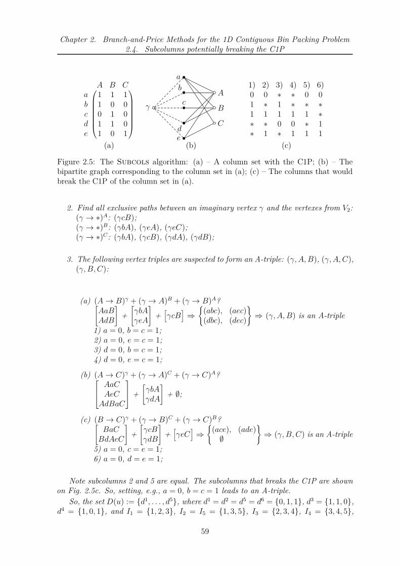
Chapter 2. Branch-and-Price Methods for the 1D Contiguous Bin Packing Problem2.4. Subcolumns potentially breaking the C1P
A B C1 1 11 0 00 1 01 1 01 0 1
abcde
(a)
a
b
c
de
A
B
C
γ
(b)
1) 2) 3) 4) 5) 6)0 0 ∗ ∗ 0 01 ∗ 1 ∗ ∗ ∗1 1 1 1 1 ∗∗ ∗ 0 0 ∗ 1∗ 1 ∗ 1 1 1
(c)
Figure 2.5: The Subcols algorithm: (a) – A column set with the C1P; (b) – Thebipartite graph corresponding to the column set in (a); (c) – The columns that wouldbreak the C1P of the column set in (a).
2. Find all exclusive paths between an imaginary vertex γ and the vertexes from V2:(γ → ∗)A: (γcB);(γ → ∗)B: (γbA), (γeA), (γeC);(γ → ∗)C: (γbA), (γcB), (γdA), (γdB);
3. The following vertex triples are suspected to form an A-triple: (γ, A,B), (γ, A, C),(γ,B, C):
(a) (A→ B)γ + (γ → A)B + (γ → B)A?[AaBAdB
]+
[γbAγeA
]+
[γcB
]⇒
{(abc), (aec)(dbc), (dec)
}⇒ (γ, A,B) is an A-triple
1) a = 0, b = c = 1;2) a = 0, e = c = 1;3) d = 0, b = c = 1;4) d = 0, e = c = 1;
(b) (A→ C)γ + (γ → A)C + (γ → C)A?AaCAeC
AdBaC
+
[γbAγdA
]+ ∅;
(c) (B → C)γ + (γ → B)C + (γ → C)B?[BaCBdAeC
]+
[γcBγdB
]+
[γeC
]⇒
{(ace), (ade)∅
}⇒ (γ,B, C) is an A-triple
5) a = 0, c = e = 1;6) a = 0, d = e = 1;
Note subcolumns 2 and 5 are equal. The subcolumns that breaks the C1P are shownon Fig. 2.5c. So, setting, e.g., a = 0, b = c = 1 leads to an A-triple.
So, the set D(u) := {d1, . . . , d5}, where d1 = d2 = d5 = d6 = {0, 1, 1}, d3 = {1, 1, 0},d4 = {1, 0, 1}, and I1 = {1, 2, 3}, I2 = I5 = {1, 3, 5}, I3 = {2, 3, 4}, I4 = {3, 4, 5},
59

Chapter 2. Branch-and-Price Methods for the 1D Contiguous Bin Packing Problem2.4. Subcolumns potentially breaking the C1P
I6 = {1, 4, 5}. Thus, the constraints to be added into CG(u) are:
a1 + (1− a2) + (1− a3) > 0
a1 + (1− a3) + (1− a5) > 0
(1− a2) + (1− a3) + a4 > 0
(1− a3) + a4 + (1− a5) > 0
a1 + (1− a3) + (1− a5) > 0
a1 + (1− a4) + (1− a5) > 0
If the cardinality of the set Ppq is acceptable then we can improve the algorithm Sub-cols by using less calls of the "all exclusive paths" procedure, refer to Algorithm 2.6.
Algorithm 2.6 (Subcols’). Determination of forbidden subcolumns.Input data: A node u, the column set {aj : j ∈ J+(u)}.Output data: D(u).
(1 ) Construct the bipartite graph B0 := (V1 := I, V2 := {1, . . . , |J+(u)|}, E0 :={(i, j) : j ∈ V2, i ∈ N(j)}).
(2 ) For each pair of vertexes p ∈ V2, q ∈ V2\{p}: p < q in B0 find all exclusive pathsAllPaths(B0, p→ q) and save these in Ppq.
(3 ) V1 := I\[(p→ q) ∩ I], V2 := {1, . . . , |J+(u)|, γ},Eγ := E0 ∪ {(i, γ) : i ∈ I}\{(γ, o), (o, r) : o ∈ (p→ q) ∩ I, r ∈ V2}.For each pair of vertexes (p→ q) ∈ Ppq build the following two graphs:Bp := (V1\N(p), V2\{p}, Eγ\{(γ, o), (o, r) : o ∈ N(p), r ∈ V2});Bq := (V1\N(q), V2\{q}, Eγ\{(γ, o), (o, r) : o ∈ N(q), r ∈ V2});If there exists a path (γ → p) in Bq and (γ → q) in Bp then (γ, p, q) builds anA-triple. Then D(u) := D(u) ∪ {d∗} withd∗
i := 0, i ∈ (p→ q) ∩ I;
d∗i := 1, i ∈ [(γ → p) ∪ (γ → q)]\[(p→ q) ∩ I];
Algorithm 2.7 (AllPaths). The all paths algorithm: the algorithm is a modificationof the depth-first search (DFS) which stores at every step a list of the traversed vertexesand the modified incidence matrix.Input data: Start S, E, and the incident matrix M .Output data: Set W of all exclusive ways between S and E.
(1 ) Push node S and matrix M to the stack, Push(S, M).(2 ) Restore the current node o and the matrix M from the stack, (o,M)← Pop(). If
o 6= ∅ then all paths from S to E are investigated and goto Exit.(3 ) If node o is equal to E then a new path from S to E is found, otherwise restore
the next node: If o = E then store this path W := W ∪ {(S → E)} and goto2. Else find each node which is incident to o, delete the incidence record betweenthem in M and push them into the stack: For all j with mj
o = 1 set mjo = mo
j = 0and Push(j, M). Goto 2.
60

Chapter 2. Branch-and-Price Methods for the 1D Contiguous Bin Packing Problem2.5. Numerical study
Note Algorithm 2.7 has an exponential time complexity and dm2 space complexitywhere d is the maximal depth of the tree.
Example 2.2. On Fig. 2.6a there is a bipartite graph which corresponds to a columnset. On Fig. 2.6b a search tree is shown which is build according to the AllPathsalgorithm for finding the all exclusive paths between nodes A and C. So, we have foundthe following paths: AaC, AaBbC, AbC, AbBaC. The dashed edges of the tree markthe cycles.
a
b
c
d
A
B
C
D
(a)
A
ba
BC
B
C
D
cb
ca
C D C
(b)
Figure 2.6: The AllPaths algorithm: (a) – A bipartite graph; (b) – A search treewhich is build for finding all exclusive paths between nodes A and C.
2.5 Numerical study
In this section we discuss numerical experiments for the CBPP-1 instances which areobtained from SPP-2 from different sources.
The algorithm was implemented as a single-threaded application in C++ basedon Visual Studio 2008, compiler version 9.0.30729, on an AMD Athlon 64 Dual Core4200+ (2.2 GHz) CPU. IBM ILOG CPLEX 12.5 was used as an LP solver. The testinstances, detailed results and source code are available on the CaPaD website2 and in[MSB13b].
In Table 2.1 the number of nodes and time are the mean values over the solvedinstances. From a rational number we take only the integer part without rounding.
Here are the following implementation issues to consider:
1. The time limit for each instance and method was set to 900 seconds.
2. For obtaining a good performance of the branch-and-price algorithms we limitthe iterations for the algorithms from Sections 2.3, 2.4 by 1000.
3. We do not consider any methods of stabilization or optimization of the columngeneration process, since this is not a subject of the research of this paper. Con-sidering of these steps may result in a better computational behavior of thebranch-and-price method.
2http://www.math.tu-dresden.de/∼capad
61

Chapter 2. Branch-and-Price Methods for the 1D Contiguous Bin Packing Problem2.6. Conclusions
4. In Table 2.1 the results for the decision problem of CBPP-1 are shown. Thedecision problem asks whether a set of items can be packed into the bins feasibly,so that the number of used bins does not exceed 20. If so then the instance iscalled feasible, otherwise infeasible.
2.6 Conclusions
Here we have proposed and studied news branch-and-price methods for the 1D con-tiguous bin packing problem.
The main theoretical and experimental observations of the paper are the following:
1. Given a column set with the consecutive 1’s property and a column which breaksthis property it is computationally not very consuming to find all the subcolumnsof the column which break the property. If we the column breaking the consecu-tive 1’s property is not given, the problem becomes computationally hard.
2. The branching strategy based on the enumeration of the columns behaves on thewhole better on feasible instances where we have to find a solution. On the otherhand the branching strategy based on the enumeration of the subcolumns is of abeneficial use for the infeasible instances where the infeasibility has to be provenby increasing the bound.
3. The following issues are subject to further study: can we model (possibly remain-ing in the linear programming) the 2D strip packing problem using two modelsof the 1D contiguous bin packing in a single formulation as we did in [MSB13a]?
2.7 Acknowledgments
We appreciate the Academic Initiative of IBM which enables many researchers all overthe world to compare their methods using state-of-the-art IBM ILOG OptimizationSoftware.
62

Chapter 2. Branch-and-Price Methods for the 1D Contiguous Bin Packing Problem2.7. Acknowledgments
Table 2.1: Results of the decision version of CBPP-1 on the 2D instances from [CJM08]:A – Branch-and-price-cols; B – Branch-and-price-subcols; n – total numberof nodes; t – total time.
A Binst opt n t opt n t
Infeasible instances00N10 1 1 0 1 1 000N15 1 1 0 1 1 000N23 1 1 0 1 1 000X23 0 - - 0 - -02N20 1 1 0 1 1 003N10 1 84 1 1 27 103N15 1 1 0 1 1 003N16 1 461 4 1 324 403N17 1 1 0 1 1 004N15 1 1 0 1 1 004N17 1 1 0 1 1 004N18 1 1 0 1 1 005N15 1 1 0 1 1 005N17 1 215 4 1 101 305X15 1 1 0 1 1 007N10 1 1 0 1 1 007N15 1 1 0 1 1 007X15 1 80 2 1 79 208N15 1 3 0 1 3 010N10 1 1 0 1 1 010N15 1 1 0 1 1 010X15 1 1 0 1 1 013N10 1 466 1 1 420 113N15 1 1 0 1 1 013X15 1 1 0 1 1 015N10 1 60 1 1 57 015N15 1 1 0 1 1 0mean 26 53 1 26 40 0Feasible instances02F17 1 10371 14 1 17415 2402F20 1 2350 5 1 7203 1502F22 1 3201 9 1 8011 2003X18 1 1280 6 1 1407 704F15 1 633 3 1 914 304F17 1 131 1 1 135 104F19 1 965 4 1 1134 504F20 1 318 7 1 510 805F15 1 382 2 1 479 205F18 1 101 1 1 108 105F20 1 415 2 1 813 407F15 1 544 2 1 1437 408F15 1 54 1 1 60 120F15 1 49 1 1 78 120X15 1 39 0 1 40 0mean 15 1389 4 15 2650 6
63


Chapter 3
Constraint ProgrammingApproaches for Orthogonal Packing
We consider the 2D orthogonal feasibility problem (OPP-2) and the 2Dstrip packing problem (SPP-2). Given a set of rectangular items, OPP-2is to decide whether all items can be orthogonally packed into the givenrectangular container; SPP-2 is to find a packing of all items occupying theminimal height of the given semi-infinite strip. We investigate the knownConstraint Programming (CP) approaches for OPP-2, in particular thedichotomy and disjunctive branching strategies and adapt 1D relaxationbounds based on linear programming (LP) into the constraint propagationprocess of the CP. Using the dichotomic search procedure the developedmethods for OPP-2 are transformed for the case of SPP-2. Numericalresults demonstrate the efficiency of the proposed strategies and of thecombination of CP and LP-based pruning rules.
3.1 Introduction
Let us consider a set of m rectangular items (wi, hi), with i ∈ I := {1, . . . , m}. The2-dimensional orthogonal packing feasibility problem (OPP-2) [FS04a, CJCM08] askswhether all the items (wi, hi) with i ∈ I can be orthogonally packed into the givencontainer (W,H) without rotations. The guillotine constraint [MAVdC10, CJM08]is not considered. All input data are positive integers, i.e., W,H ∈ Z+, and wi ∈{1, . . . ,W}, hi ∈ {1, . . . , H} for i ∈ I. All problems which are introduced in this papercan be easily generalized for higher dimensions, so sometimes they will be mentionedwithout an indication of the dimension.
In the case when the items cannot be packed into the container, it is enough todeclare a negative response, otherwise the solution is a feasible packing layout withthe items allocated orthogonally and non-overlapped within the container. OPP is asubproblem in solution methods for orthogonal bin packing (BPP) and knapsack prob-lems (OKP) [FS04a, BB07, PS07]. OPP is polynomially equivalent to the orthogonalstrip-packing problem (SPP) [Hif98, AVPT09, KIN+09]. The latter problem can besolved by the dichotomic search, see Section 3.4.8.
65

Chapter 3. Constraint Programming Approaches for Orthogonal Packing3.1. Introduction
3.1.1 Formulation of OPP and overview of solution methods
Suppose we have a coordinate system with origin (0, 0) matched with the left bottompoint of the container whose x, y-axis are associated with its W,H-sides, respectively.
Let us introduce sets of variables X := {xi : i ∈ I} and Y := {yi : i ∈ I} whichrepresent the allocation points for the items in the (0, x)-, (0, y)-directions, respectively.An assignment of certain values to the variables is feasible in the sense of OPP-2, ifthe following constraints are satisfied:
xi + wi ≤ xj ∨ xj + wj ≤ xi∨
yi + hi ≤ yj ∨ yj + hj ≤ yi, (i, j) ∈ I × I : i < j; (3.1)
0 ≤ xi ≤W − wi, i ∈ I; (3.2)
0 ≤ yi ≤ H − hi, i ∈ I; (3.3)
xi, yi ∈ Z+, i ∈ I. (3.4)
It is assured that the items do not overlap, the constraints (3.1), and lie within thecontainer, the constraints (3.2), (3.3). If there exist values of the variables so thatthe constraints (3.1)-(3.4) are satisfied then the instance is called feasible, otherwiseinfeasible.
So, the above tiny formulation [CJM08, PS07] is a valid non-linear integer modelof OPP-2. In order to solve OPP-2 in this formulation, some constraint programmingmethods are successfully applied, which leads to the best results today [CJM08, SO08,Sim08, BCDP11, PS07, KMP10]. The approaches can be divided into two groups, thefirst one fixes the coordinates of the items [CJM08, SO08, Sim08], the other fixes themutual position of the items [PS07, SO08, Sim08, BCDP11].
One of the reasons of the success of the constraint programming paradigm is theefficient constraint propagation technique. In every node of the search tree it tries todecide whether the set of the constraints (3.1)-(3.4) is consistent. In other words, ittries to prove the infeasibility of the current partial solution when certain values areassigned to some variables or domains of possible values of the variables are restricted.If an inconsistency of the set of constraints cannot be proven then the procedure triesto reduce the domain of possible values for the variables.
There exist many ILP models [Bea85, Pad00, BB07, BKRS09] for OPP-2 basedon different representations of a feasible solution. Exact solution of OPP-2 in theabove ILP formulations is difficult because of the weak LP bounds of some models[Pad00], quadratic number of intersection variables, and/or pseudo-polynomial numberof position-indexed variables [Bea85, BB07] in some models.
Modeling with rotations
Rotation of items by 90◦ withing (3.1)-(3.4) can by modeled by an introduction ofbinary variables ri, i ∈ I which indicate in case of ri = 1 that item i is rotated by 90◦.
66

Chapter 3. Constraint Programming Approaches for Orthogonal Packing3.1. Introduction
The resulting model is:
xi + wi(1− ri) + hiri ≤ xj∨
yi + hi(1− ri) + wiri ≤ yj (i, j) ∈ I × I : i 6= j; (3.5)
0 ≤ xi ≤ W − wi(1− ri)− hiri, i ∈ I; (3.6)
0 ≤ yi ≤ H − hi(1− ri)− wiri, i ∈ I; (3.7)
xi, yi ∈ Z+, i ∈ I. (3.8)
ri ∈ {0, 1}, i ∈ I. (3.9)
Further in this paper we consider OPP without rotations.
3.1.2 Relaxations and bounds for OPP
In order to decide whether an instance of OPP is infeasible sometimes it is enoughto solve a relaxation. These are of different kinds, i.e., volume bounds, dual-feasiblefunctions (DFF) [CAVdC10a], conservative scales (CS) [FS04b, BKRS13], 1D bar re-laxations [Sch99, BKRS09], and relaxations of ILP models. All of the mentioned boundsare discussed in [BKRS13].
Conservative scales (CS) are modified items sizes such that if the OPP instance isfeasible then it is also feasible with the modified sizes. Thus, the volume bound for themodified instances is valid for the original instance. In fact, CS are valid inequalitiesfor a certain 0-1 knapsack polyhedron.
Dual feasible functions (DFFs) produce a subset of CS [BKRS13]. The concept ofDFF has been firstly used to obtain algorithmic lower bounds for bin packing problems[Lue83]. Most of the methods proposed for computing DFFs are polynomial and rely onknown families of functions [CAVdC10a, CCM07, FS01, FS04b, CAVdC10b]. For the2D problems, DFFs are rather weak [BKRS13] in contrast to 3D problems. So-calledmaximal CS cannot always be obtained by DFFs; corresponding methods are proposedin [BKRS13].
The 1D bar relaxation [Sch99, BKRS09] is a double relaxation of OPP-2. Firstly, wedivide the container and items into 1D bars with unit thickness. Further we formulatethe minimization problem over the number of used 1D bars which are needed to packall the split items without repetition in a single bar. Secondly, we formulate a set-partitioning model of the above 1D problem, continuously relax it, and solve it by thecolumn generation method [KZ51, GG61, GG63]. The 1D bar relaxation bound canbe further strengthened [BKRS09] by the additional information, i.e., from a probingprocedure which restricts the set of items combined in the bars.
Up to know, there were only few efforts to use the bar relaxation in an algorithm forOPP. In [BR13] the 1D bar relaxation bounds were integrated into a modified interval-graph algorithm from [FS04a]. The bound was also tightened in each dimension usingthe overlapping information from the graphs. This extended information was usedin the column generation. The tightened bound was applied in every node of thebranching tree.
67

Chapter 3. Constraint Programming Approaches for Orthogonal Packing3.2. An overview of the algorithm of Clautiaux et al.
3.1.3 Our contributions
In order to solve OPP we investigate and modify the state-of-the-art constraint pro-gramming approaches [CJM08, SO08, Sim08]. We compare some known branchingstrategies, e.g., contour, interval, disjunctive, and propose new dichotomy and inter-section strategies, in Section 3.4. In Section 3.5 we propose new pruning rules basedon the tightened 1D bar relaxations [Sch99, BKRS09] of various kinds, e.g., intervals,forbidden pairs, and an advanced bar relaxation. The input data for the bar relaxationis obtained from the local partial solution, the information from the constraint prop-agation procedure, and the relative positions of the items in the container. The finalpart of the paper reports numerical results and conclusion.
3.2 An overview of the algorithm of Clautiaux et
al.
In this section we consider the algorithm of Clautiaux et al. [CJM08] and give somenecessary definitions.
3.2.1 Basic definitions
Clautiaux et al. [CJM08] proposed an algorithm for OPP-2 which solves it as twoscheduling problems. Let be given sets AW := {AW
1 , . . . , AWm } andAH := {AH
1 , . . . , AHm}
of activities and two types of resources of H and W units. Each of the activities Adi
with d ∈ {W,H} and i ∈ {1, . . . , m} has its time interval [startdi , enddi ) where the
activity Adi can occur. startdi designates the earliest point of time where activity Ad
i
can start, and enddi is the latest point of time where activity Ad
i can end. Each activityAW
i ∈ AW , AHi ∈ AH has its level of consumption hi of the resource H , wi of the
resource W , and durations wi, hi, respectively. A schedule is called continuous, if inthe schedule each activity is not interrupted during the execution, and cumulative, ifall activities are consuming the same resource. At every discrete point of time theresource capacity is limited by a certain value and must not be exceeded.
Let us now superpose each feasible start time point of the activity AWi with the
variables fromX, and AHi with the variables from Y then xi ∈ [startWi , end
Wi −wi]∩Z =
[xi, xi] ∩ Z and yi ∈ [startHi , endHi − hi] ∩ Z = [y
i, yi] ∩ Z, i.e., [xi, xi] and [y
i, yi] are
feasible domains for the variables. If we now assume that xi = yi
:= 0, xi := W − wi,yi := H − hi with i ∈ I, both schedules are cumulative and continuous, and if theconstraints (3.1) for the variables from X and Y are satisfied then the model based ontwo scheduling problems connected through the constraints (3.1) is a feasible model ofOPP [CJM08].
The formulation of OPP-2 modeled by two scheduling problems is solved by thebranch-and-bound method, i.e., a branching tree T := (V,E) is built. Two nodesu, v ∈ V differ by the local set of branching restrictions. Based on the kind of branchingrestrictions, various branching strategies are possible.
68

Chapter 3. Constraint Programming Approaches for Orthogonal Packing3.2. An overview of the algorithm of Clautiaux et al.
3.2.2 Branching strategy
Let u ∈ V be a node of the branching tree T . Node u is also called a subproblem. If avalue is assigned to a variable then the variable is called fixed. Let
Iux := {i ∈ I : xi 6= xi}, Iu
y := {i ∈ I : yi6= yi},
be the index sets of the unfixed variables from X and Y , respectively. Herewith,Iu
x := I\Iux and Iu
y := I\Iuy are the index sets of fixed variables.
The original branching strategy [CJM08] is a two-step approach where the variablesfrom X are fixed first, and the variables from Y are fixed next, see Algorithm 3.1. Thatmeans, if only Iu
x = ∅ then we start to branch on the variables from Y .An important issue is the selection of a branching variable from the unfixed ones,
steps 1 and 2. It is based on the following observation. If we pack all the large items atfirst instead of packing all the items in an arbitrary order then we can rapidly obtainthe inconsistency of the system (3.1)-(3.4), if any, because we do not lose much effortduring the allocation of the small items.
As soon as a variable for branching is selected, it is fixed to the value which is equalto its lower bound (the first branch) or the lower bound for its domain is increased (thesecond branch), see step 4.
For describing the algorithm in a simpler way let us introduce the order of thevariables, so xi ≺ xj ⇔ i < j and yi ≺ yj ⇔ i < j for i, j = 1, . . . , m.
Algorithm 3.1 (FixMin). Creation of two descendants of a node u ∈ V according tothe original branching strategy [CJM08].Input data: A node u ∈ V .Output data: Descendant nodes v1, v2.
(1 ) If Iux 6= ∅ then set:
P := {xi ∈ X : i ∈ Iux , wihi = max{wihi : i ∈ Iu
x}},
and goto step 3.(2 ) If Iu
y 6= ∅ then set:
P := {yi ∈ Y : i ∈ Iuy , wihi = max{wihi : i ∈ Iu
y }},
and goto step 3, else goto Exit.(3 ) Select the variable with the smallest lower bound for its domain and then with the
lowest index:
p := min≺{p ∈ argmin{p : p ∈ P}}.
(4 ) Definition of the descendant nodes:
v1: p := p (fixation of the variable);v2: p := p + 1 (p is fixed later).
69

Chapter 3. Constraint Programming Approaches for Orthogonal Packing3.3. Minor modifications
The following statement is true.
Lemma 3.1. The depth of the branching tree by FixMin is O(m(W +H)).
Proof. Each item is tried to be fixed in each feasible position in the (0, x)-direction,mW possible variants, and in the (0, y)-direction, mH possible variants. Since foreach feasible position we have one branch then the depth of the branching tree isO(m(W +H)).
3.3 Minor modifications
In this section we consider minor modifications of the original algorithm which areused either in each node of the branching tree as raster points and local preprocessingor only in the root node as an initial preprocessing. Let E := (m,W,H,w, h) be anOPP-2 instance.
3.3.1 Raster points
It is often excessive to consider for a variable p each point from its domain [p, p]∩Z. Forinstance, if we have only three activities with the durations 4, 7, 9 then a schedule withthe starting point 5 has never to be considered. The points which are of interest arecalled raster points [Sch08] and are calculated, e.g., for the (0, x)-direction as follows:
Rx(N) := {0 ≤ x ≤ N : x =∑
i∈I
wiai, ai ∈ {0, 1}, i ∈ I}.
In the mentioned book, the author proposes an approach for a reduction of thenumber of raster points by the consideration of reduced set of raster points.
Rx(N) := {max{k ∈ Rx(N) : k ≤ N − r} : r ∈ Rx(N)}.
In order to obtain raster points which are situated to the left and right of a pointα, let us consider the following definitions:
Rx(α,N) := max{β ∈ Rx(N) : β ≤ α}, Rx(α,N) := min{β ∈ Rx(N) : β ≥ α}
Similarly, we define Ry(α,N) and Ry(α,N) for the (0, y)-direction. Let designateRx(α) := Rx(α,W ) and Ry(β) := Ry(β,H).
Further we propose some branching strategies and pruning approaches which useraster points and a reduced set of raster points, see Sections 3.4.1, 3.4.2, 3.4.3, 3.4.8.
3.3.2 Initial preprocessing
The procedure of an initial preprocessing is performed only once for the root node.The idea of the procedure is to eliminate some symmetrical and equivalent solutionswhich satisfy the constraints (3.1)-(3.4). The results of the procedure are additional
70

Chapter 3. Constraint Programming Approaches for Orthogonal Packing3.3. Minor modifications
constraints which are appended to the model (3.1)-(3.4) or replace some of its con-straints. A similar procedure was proposed in [MMBS11] for the 1D contiguous binpacking problem (CBPP-1). For further restrictions refer to papers [BM03, CCM07].
In order to eliminate the solutions which are obtained through the symmetry overthe vertical and horizontal lines going over the geometrical center of the container weapply:
xi∗ ≤⌊W − wi∗
2
⌋+ 1, yi∗ ≤
⌊H − hi∗
2
⌋+ 1, i∗ := min{i ∈ Q},
where Q := {i ∈ I : wihi = max{wkhk : k ∈ I}} is the set of the item indexes withthe largest area. Herewith, according to the FixMin strategy the item i∗ is fixed first,see steps 1 and 3 of Algorithm 3.1. This fact will be used in Section 3.5.3.
Let
Fx := {(i, j) ∈ I × I : i < j, wi + wj > W},
Fy := {(i, j) ∈ I × I : i < j, hi + hj > H}
be the sets of item pairs which do not fit together over the (0, x)-, and (0, y)-directions,respectively. Then instead of (3.1), the following constraints are applied:
xi + wi ≤ xj ∨ xj + wj ≤ xi, (i, j) ∈ Fy; (3.10)
yi + hi ≤ yj ∨ yj + hj ≤ yi, (i, j) ∈ Fx; (3.11)
xi + wi ≤ xj ∨ xj + wj ≤ xi∨
yi + hi ≤ yj ∨ yj + hj ≤ yi, (i, j) ∈ (I × I)\(Fx ∪ Fy) : i < j. (3.12)
If two items i and j are identical, i.e., wi = wj and hi = hj then we apply thefollowing constraints:
xi < xj∨
xi = xj∧yi + hi ≤ yj, (i, j) ∈ I × I : i < j, wi = wj, hi = hj.
Instead of (3.2) and (3.3), the following constraints are applied:
0 ≤ xi ≤ Rx(W − wi), i ∈ I; (3.13)
0 ≤ yi ≤ Ry(H − hi), i ∈ I. (3.14)
3.3.3 Local preprocessing
This type of the preprocessing is performed for each node of the branching tree. Themain idea is to reduce the domain of the variables to a possibly small size. In terms ofthe constraint programming paradigm the local preprocessing is called constraint prop-agation [Apt03]. Since for the solution of our model we use ILOG CP (see Section 3.6for further details), the local preprocessing is done automatically for each node of thebranching tree after its creation.
71

Chapter 3. Constraint Programming Approaches for Orthogonal Packing3.4. New branching strategies
3.4 New branching strategies
In this section we review some known and propose new strategies which are based ondifferent principles. First group of the branching strategies fixes coordinates of theitems or divides the domain of the variables. The other group branches on the mutualpositions of the items, e.g., overlapping relations. The description of the new strategiesuses notations from Sections 3.1, 3.2. For a numerical study of the strategies, refer toSection 3.6.
Strategies FixMin, FixMinR and Contour from this section fix a variable orincrease the lower bound of its domain in each branch. In that case we will use thenotation of a contour and a block-structure. The related but different notions of thecontour were proposed in [Sch95] for 2D packing layouts. Let u ∈ V be a node of thebranching tree and Iu
x (t) := {i ∈ Iux : t ∈ [xi, xi + wi)} be the item set with the fixed
x-coordinate whose x-projection intersects a given point t ∈ [0,W ).
Definition 3.1. The X-contour Cux corresponding to a node u ∈ V is the graph of the
function:
Cux (t) :=
∑
i∈Iux (t)
hi, t ∈ [0,W ).
Cux (t) is a step function with, in general, some discontinuity points in (0,W ). Let
the ordered sequence {χuk}
qux +1
k=1 contain exactly all the discontinuity points and theborder values, such that 0 = χu
1 ≤ χu2 ≤ . . . ≤ χu
qux +1 = W , i.e.,
limt→χx
k−0Cu
x (t) 6= limt→χx
k+0Cu
x (t) = Cux (χx
k), k ∈ {2, . . . , qux},
where qux + 1 is the number of jump discontinuity points in (0,W ) plus two border
points. For convenience, let
Cux (W ) := lim
t→W −0Cu
x (t).
Definition 3.2. If C(χxk) > C(χx
k+1), ∀k ∈ Qux := {1, . . . , qu
x} then the X-contour iscalled monotonically decreasing or monotone.
Remark 3.1. Similarly, we define the Y -contour Cuy corresponding to a node u ∈ V .
Assigned to an interval [χuk , χ
uk+1) with k ∈ Qu
x we define a vertical block as therectangle [χu
k , χuk+1)× [0, H) lying above Cu
x , see Figure 3.7.
Definition 3.3. The k-th block corresponding to a contour Cux is the rectangle [χx
k, χxk+1)×
[Cux(χu
k), H), denoted by (χxk, λ
xk, ρ
xk) where λx
k = H − Cux (χx
k), and ρxk = χx
k+1 − χxk.
In terms of scheduling, the k-th block represents the non-used resource duringthe period [χx
k, χxk+1). Papers [BSM08, MMBS11] define a related notion of a slice
describing the complete layout in the period [χxk, χ
xk+1). Here a block is a part of a
slice.
72

Chapter 3. Constraint Programming Approaches for Orthogonal Packing3.4. New branching strategies
Definition 3.4. The sequence of the vertical blocks {(χxk, λ
xk, ρ
xk)}qu
x
k=1 is called the ver-tical block-structure corresponding to a contour Cu
x and is denoted by S‖(u).
Remark 3.2. Similarly, we define the horizontal block-structure S=(u) consisting ofthe horizontal blocks {(χy
k, λyk, ρ
yk)}qu
x
k=1 corresponding to a contour Cuy .
In the strategies Dichotomy and Interval we change the lower and the upperbounds for the domain of a variable to branch. A principally different strategy isDisjunctive. In every branch we fix a mutual item position.
3.4.1 Original branching strategy with raster points
Here we try to heuristically reduce the large branching depth of the FixMin strategycaused by choosing individual values for the variables. For that purpose we bring thereduced set of raster points from Section 3.3.1 into FixMin.
In the proposed strategy we change step 4 of Algorithm 3.2 as follows. While anode u ∈ V of the branching tree is processed, two descendant nodes are created wherein the second descendant v2 we set the lower bound for the variable domain to the nextraster point, see Algorithm 3.2.
Let the type of a variable p ∈ X ∪ Y be determined in the following algorithms by
d(p) :=
x, if p ∈ X;
y, if p ∈ Y.
Algorithm 3.2 (FixMinR). Creation of two descendants of a node u ∈ V accordingto the improved FixMin.Input data: A node u ∈ V .Output data: Descendant nodes v1, v2.
(1-3) Same as in Algorithm 3.1.(4) Definition of the descendant nodes:
v1: Same as in Algorithm 3.1;v2: p := Rd(p)(p+ 1) (p is fixed later).
The worst case depth of the branching tree by FixMinR remains the same as byFixMin.
Remark 3.3. The X-contour generated by FixMin and FixMinR is, in general,non-monotonic.
3.4.2 Contour branching strategy
Here we propose a branching strategy which is a modification of the contour concept[Sch95, MMV03] for the 1D case. This approach is a classical branching strategy, amodification of which was used in the algorithm [MMBS11] for the solution of CBPP-1.
73

Chapter 3. Constraint Programming Approaches for Orthogonal Packing3.4. New branching strategies
Similarly to FixMin and FixMinR, the approach starts to fix the variables fromX. After all variables from X are fixed, the approach omits the information concerningthe fixed variables from X, and fixes the variables from Y , see Algorithm 3.3.
The strategy sequentially builds a contour. On each step we select the earliest blockin which at least one item from the unfixed ones can be fixed. Further we decide whichitem is fixed within the block (one node for each choice). Additionally, we create anode in which we demand that none of the unfixed items is fixed within the selectedblock, see step 3 of Algorithm 3.3.
Algorithm 3.3 (Contour). Creation of descendants of a node u ∈ V according tothe contour principle.Input data: A node u ∈ V , block-structures Sx
‖ (u), Sy‖ (u).
Output data: Descendant nodes v0, . . . , vn.
(1 ) If Iux 6= ∅ then set:
k∗ := argmin{χxk : ∃i ∈ Iu
x , hi ≤ λxk}, P := {xi ∈ X : hi ≤ λx
k}.
goto step 3.(2 ) If Iu
y 6= ∅ then set:
k∗ := argmin{χyk : ∃i ∈ Iu
y , wi ≤ λyk}, P := {yi ∈ Y : wi ≤ λy
k}.
goto step 3, else Exit.(3 ) Definition of the descendant nodes:
v0: ∀p ∈ P set p := Rd(p)(χd(p)k∗ + 1).
For j = 1, . . . , |P|:
vj: p = p := χd(p)k∗ .
Some papers [Sch95, MMBS11] discuss anti-symmetry rules for Contour in orderto eliminate vertical and horizontal equivalent solutions, also with respect to identicalitems, etc. Here we do not use them.
Lemma 3.2. The depth of the branching tree by Contour is O(m).
Proof. On each depth one item is fixed. Thus, the depth of the tree is O(m).
Remark 3.4. The contour generated by Contour is monotone.
3.4.3 Dichotomy
Here we propose a new branching strategy. The idea is to obtain a well balanced and asmall branching tree. Now, instead of checking each coordinate value from the domainas by FixMin we try to divide the domain of a branching variable into two intervals.
First of all, on each step we select a variable to branch. Here we either select thevariable as by FixMin or select the variable with the biggest domain over the unfixedones which results in two different approaches, see step 3 of Algorithm 3.4. If a variableg is selected, two branches are created where g is restricted to the first half or to thesecond half of the interval [g, g], see step 4.
74

Chapter 3. Constraint Programming Approaches for Orthogonal Packing3.4. New branching strategies
Algorithm 3.4 (Dichotomy). Creation of two descendants of a node u ∈ V accordingto the dichotomy principle.Input data: A node u ∈ V .Output data: Descendant nodes v1, v2.
(1-2) Same as in Algorithm 3.1.(3) Dichotomy(coordinate): Step 3 of Algorithm 3.1.
Dichotomy(interval): Select the variable with the biggest domain and then withthe lowest index:
p := min≺{p ∈ argmax{p− p : p ∈ P}}.
(4) Definition of the descendant nodes:
v1 : p := Rd(p)(⌊p+ p
2⌋); v2 : p := Rd(p)(⌊
p + p
2⌋+ 1).
Lemma 3.3. The depth of the branching tree by Dichotomy is O(m(logW +logH)).
Proof. Each item is tried to be fixed in every interval after division in half. The depthof the branching subtree for an item i ∈ I is equal to the number of divisions in the(0, x)-direction of the interval xi − xi which is equal in the worst case to W , and H inthe (0, y)-direction. Since the number of divisions of W is logW (for H is logH) andthese divisions are done for each item i ∈ I then the depth is O(m(logW +logH)).
3.4.4 Interval
In [SO08, Sim08] different strategies are discussed. The combination of the naive andthe xtheny strategies from the paper yields the FixMin strategy. The most successfulapproach according to that paper is the interval strategy. It was firstly proposed in[BCDP11] for the perfect square packing problem.
The interval strategy consists in splitting of the domain of the variables from Xinto intervals then fixing the values for them, followed by splitting the domain of thevariables from Y , and finally fixing the values for them. The splitting of the domainfor a variable depends on the size of the corresponding item. It should be chosensmall enough so that a mandatory part of the item occurs in each interval. In theoriginal interval strategy, one third of the item size occurring obligatory in one ofthe split intervals, yields the best results [Sim08]. In comparison to interval, here weuse Dichotomy when the intervals are too small to be split, see steps 1 and 2 ofAlgorithm 3.5.
Algorithm 3.5 (Interval). Creation of descendants of a node u ∈ V according tointerval principle [Sim08].Input data: A node u ∈ V , a ratio r (here and further r = 0.3).Output data: Descendant nodes v0, . . . , vn.
75

Chapter 3. Constraint Programming Approaches for Orthogonal Packing3.4. New branching strategies
(1 ) If Iux 6= ∅ then:
Q := {i ∈ Iux : xi−xi ≥ ⌈rwi⌉}, P := {xi ∈ X : i ∈ Q, wihi = max
i∈Q{wihi}}
else goto 2. If Q 6= ∅ then goto step 3, else Dichotomy.(2 ) If Iu
y 6= ∅ then:
Q := {i ∈ Iuy : yi−yi
≥ ⌈rhi⌉}, P := {yi ∈ Y : i ∈ Q, wihi = maxi∈Q{wihi}}
else goto Exit. If Q 6= ∅ then goto step 3, else Dichotomy.(3 ) Select the variable with the greatest domain and then with the lowest index:
p := min≺{p ∈ argmax{p− p : p ∈ P}}.
(4 ) Definition of the descendant nodes:If d(p) = x then set s := ⌈rwi⌉ with i ∈ Iu
x ∧ xi = p, else set s := ⌈rhi⌉ with
i ∈ Iuy ∧ yi = p. For j = 1, . . . , ⌈
p−p
s⌉ create:
vj : p := p+ (j − 1)s; p := min{p+ js− 1, p}.
Lemma 3.4. The depth of the branching tree by Interval is O(m +m∑
i=1(log rwi +
log rhi)).
Proof. In the worst case we divide the interval for each item, O(m), and then fix theitems within the intervals according to Dichotomy which are equal in this case torwi and rhi, respectively, hence O(m+
∑mi=1(log rwi + log rhi)).
3.4.5 Disjunctive
This strategy is based neither on the coordinate interval division nor on the assignmentof coordinate variables as before. It is principally another strategy which iterativelyfixes the set of all possible mutual positions for a pair of items.
Let l, r, b, t ∈ N be such l < r < b < t and Rij ⊆ {l, r, b, t} be the set whichrepresents the possible mutual locations of items i, j ∈ I with i < j, i.e.,
Rij = {l} ⇔ xi + wi ≤ xj , Rij = {r} ⇔ xj + wj ≤ xi,
Rij = {b} ⇔
xi + wi > xj ,
xj + wj > xi,
yi + hi ≤ yj,
Rij = {t} ⇔
xi + wi > xj ,
xj + wj > xi,
yj + hj ≤ yi.
In Figure 3.1a we see the dimensions of an item j. Figures 3.1b-3.1e show by the hatchedareas the feasible locations of the left-bottom corner of the item j for Rij = l, r, b, t,respectively. Now, we associate with each node u ∈ V the set R(u) := {Rij : i <j, i, j ∈ I} of relations for the item pairs.
76

Chapter 3. Constraint Programming Approaches for Orthogonal Packing3.4. New branching strategies
j
(a) Item j
i
W − wj
H−h
j
(b) Rij = {l}
i
xi − wj
H−h
j
(c) Rij = {r}
i
xi − wj
H−h
j
(d) Rij = {b}
i
xi − wj
y i−h
j
(e) Rij = {t}
Figure 3.1: Mutual locations of the items i and j. The areas where the left-bottomarrangement point of the item j can be allocated are marked by hatching.
In order to prioritize item pairs selected for branching let us introduce a pair or-dering denoted by the symbol ⊐. Suppose (p, q), (r, k) ∈ I × I: p < q and r < k. So,(p, q) ⊐ (r, k), iff wphp > wrhr∨ (wphp = wrhr∧wqhq > wkhk)∨ (wphp = wrhr∧wqhq =wkhk ∧ p < r).
The main idea of the disjunctive strategy [Sim08] is to fix a relation for every itempair, see Algorithm 3.6. After a pair is selected, see steps 1 and 2, we select a relationto fix for this pair, step 3. At last, when every item pair got a relation, a packing layout(item coordinates) can be computed. If the items lie within the container bounds thenthe layout is feasible.
Algorithm 3.6 (Disjunctive). Creation of two descendants of a node u ∈ V accord-ing to the disjunctive principle.Input data: A node u ∈ V .Output data: Descendant nodes v1, v2.
(1 ) If ∃Rij ∈ R(u) : |Rij| > 1 then set:
P := {(i, j) ∈ I × I : i < j, |Rij| > 1},
else goto Exit.(2 ) Select the pair to branch:
(i, j) := min⊐
{(i, j) : (i, j) ∈ P}.
(3 ) Definition of the descendant nodes:Set f := min{k : k ∈ Rij , Rij ∈ R(u)} (note that we assume the orderingl < r < b < t). Create:
v1 : R(v1) := R(u) ∧Rij = {f}; v2 : R(v2) := R(u) ∧ Rij = Rij\{f}.
Once we have fixed all mutual locations of the items, the domain of variables fromX, Y can still contain not just a single value. It depends on the quality of the localpreprocessing procedure, see Section 3.3.3. Note that the local preprocessing procedureis preformed for every node after its creation. Several values of a variable from X, Ycan also be feasible for the model. In our case after all relations are fixed we do notbranch variables X, Y to a single value.
The following statement is true.
77

Chapter 3. Constraint Programming Approaches for Orthogonal Packing3.4. New branching strategies
Rij = {l, r, b, t}
Rij = {l}Rij = {r, b, t}
Rij = {r}Rij = {b, t}
Rij = {b} Rij = {t}le
ft
¬left
right
¬rig
ht
bott
om to
p
Figure 3.2: Binary branching tree corresponding to Disjunctive.
Theorem 3.5. If ∀i, j ∈ I : i < j, |Rij | = 1 and the system (3.1)-(3.4) holds then thecorresponding OPP-2 instance is feasible.
Lemma 3.6. The depth of the branching tree by Disjunctive is O(m2).
Proof. On each depth of the branching tree we fix one of the constant number ofrelations for a pair of items. Herewith, the depth of the tree is not larger than thenumber of pairs, O(m2).
3.4.6 Partition
As we can see at the Disjunctive strategy the decision that the projections of twoitems are partitioned over the (0, x)-, or over the (0, y)-direction is made only in thedepth of the branches. In some cases it would be better to assert the disjoint state ofthe items over one of the axis at first steps. The decision that projections of the itemsare disjoint can help, e.g., to strength some of the pruning rules as, i.e., LP-pair (forthe pruning rules refer to Section 3.5).
Let px, py, l, r, b, t ∈ N and Rij ⊆ {px, py, l, r, b, t} be the set which represents thepossible mutual locations of items i, j ∈ I with i < j, i.e.,
Rij = {px} ⇔
[xi + wi ≤ xj ,xj + wj ≤ xi,
Rij = {py} ⇔
[yi + hi ≤ yj,yj + hj ≤ yi,
Rij = {l} ⇔ xi + wi ≤ xj , Rij = {r} ⇔ xj + wj ≤ xi,
Rij = {b} ⇔ yi + hi ≤ yj, Rij = {t} ⇔ yj + hj ≤ yi.
In Figure 3.3 we show by the hatched areas the feasible locations of the left-bottomarrangement point of the item j for Rij = px, py, l, r, b, t, respectively. Now we associatewith each node u ∈ V the set R(u) := {Rij : i < j, i, j ∈ I} of relations for the itempairs. The item pairs have an ordering relation defined by ⊐ as in Section 3.4.5.
Let R := {R ⊆ {px, py, l, r, b, t} : |R| > 1 ∨R = {px} ∨R = {py}} be the set of allitem sets with no or px−py fixed relations. The main idea of the partition strategy is todecide at first steps that projections of two items without a fixed relation are disjointover one of the axis, see Algorithm 3.7. After a pair is selected, see steps 1 and 2,we assert that the projections of the item pair do not overlap over the (0, x)-direction,
78

Chapter 3. Constraint Programming Approaches for Orthogonal Packing3.4. New branching strategies
i
W − wj
H−h
j
(a) Rij = {px}
i
xi − wj
y i−h
j
(b) Rij = {py}
i
xi − wj
H−h
j
(c) Rij = {b}
i
xi − wj
y i−h
j
(d) Rij = {t}
Figure 3.3: Possible mutual locations of the items i and j according to Partition.The areas where the left-bottom arrangement point of the item j can be allocated aremarked by hatching. The size of the item j is depicted in Figure 3.1a. Rij = {l} andRij = {r} are depicted in Figure 3.1b and 3.1c.
the first branch, or over the (0, y)-direction, the second branch. When this decision ismade, the further partition is followed in the leafs, see step 3.
Algorithm 3.7 (Partition). Creation of two descendants of a node u ∈ V accordingto the partition principle.Input data: A node u ∈ V .Output data: Descendant nodes v1, v2.
(1 ) If ∃Rij ∈ R(u) : Rij ∈ R then set:
P := {(i, j) ∈ I × I : i < j, Rij ∈ R},
else goto Exit.(2 ) Selection of the pair to branch:
(i, j) := min⊐
{(i, j) ∈ P}.
(3 ) Definition of the descendant nodes:If {px, py} ⊂ Rij then
v1 : R(v1) := R(u) ∧Rij = {px}; v2 : R(v2) := R(u) ∧Rij = {py}.
If Rij = {px} then:
v1 : R(v1) := R(u) ∧Rij = {l}; v2 : R(v2) := R(u) ∧Rij = {r}.
If Rij = {py} then:
v1 : R(v1) := R(u) ∧Rij = {b}; v2 : R(v2) := R(u) ∧ Rij = {t}.
For the binary branching tree of the Partition refer to Figure 3.4. The followingstatement is true.
Theorem 3.7. If ∀i, j ∈ I : i < j, |Rij | = 1 and the system (3.1)-(3.4) holds then thecorresponding OPP-2 instance is feasible.
Lemma 3.8. The depth of the branching tree by Partition is O(m2).
Proof. We fix at most six relations for every pair which make in sum 6m2 branches.Herewith the depth of the tree is O(m2).
79

Chapter 3. Constraint Programming Approaches for Orthogonal Packing3.4. New branching strategies
Rij = {px, py, l, r, b, t}
Rij = {px} Rij = {py}
{l} {r} {b} {t}
left
right
bott
om to
p
Figure 3.4: Binary branching tree corresponding to Partition.
3.4.7 Intersection
In contrast to Partition here we propose a branching strategy where we decidewhether an item pair projection intersects one of the axis.
Let ix, ix, iy, iy, l, r, b, t ∈ N and Rij ⊆ {ix, ix, iy, iy, l, r, b, t} be the set which repre-sents the possible mutual locations of items i, j ∈ I with i < j, i.e.,
Rij = {ix} ⇔
xi < xj + wj,
xj < xi + wi.Rij = {ix} ⇔
[xi + wi ≤ xj ,xj + wj ≤ xi,
Rij = {iy} ⇔
yi < yj + hj ,
yj < yi + hi.Rij = {iy} ⇔
[yi + hi ≤ yj,yj + hj ≤ yi,
The other mutual positions of the items corresponding to Rij = {l}, {r}, {b}, {t} is thesame as in Partition, see Section 3.4.6.
Figure 3.5 shows by the hatched areas the feasible locations of the left-bottomarrangement point of the item j for Rij = {ix}, {ix}, {iy}, {iy}, respectively. For theother values of Rij refer to Figure 3.3. Now we associate with each node u ∈ V the setR(u) = {Rij : i < j, i, j ∈ I} of relations for the item pairs. The item pairs have anordering relation defined by ⊐ as in Section 3.4.5.
i
xi − wj
H−h
j
(a) Rij = {ix}
i
W − wj
H−h
j
(b) Rij = {ix}
i
W − wj
H−h
j
(c) Rij = {iy}
i
xi − wj
y i−h
j
(d) Rij = {iy}
Figure 3.5: Possible mutual locations of items i and j according to Intersection.The areas where the left-bottom arrangement point of item j can be allocated aremarked by hatching. Item j size is depicted in Figure 3.1a. Rij = {l}, Rij = {r} aredepicted in Figure 3.1b and 3.1c, Rij = {b}, Rij = {t} are depicted in Figure 3.3c and3.3d
.
80

Chapter 3. Constraint Programming Approaches for Orthogonal Packing3.4. New branching strategies
Let
R = {R ⊆ {ix, ix, iy, iy, l, r, b, t} : |R| > 1∨R = {ix}∨R = {ix}∨R = {iy}∨R = {iy}}
be the set of all item sets with no or one of ix, ix, iy or iy fixed relations. The mainidea of the partition strategy is to decide at first steps that projections of two itemswithout fixed relations overlap over one of the axis, see Algorithm 3.8.
Algorithm 3.8 (Intersection). Creation of two descendants of a node u ∈ V ac-cording to the partition principle.Input data: A node u ∈ V .Output data: Descendant nodes v1, v2.
(1 ) If ∃Rij ∈ R(u) : Rij ∈ R then set:
P := {(i, j) ∈ I × I : i < j, Rij ∈ R},
else goto Exit.(2 ) Selection of the pair to branch:
(i, j) := min⊐
{(i, j) : (i, j) ∈ P}.
(3 ) Definition of the descendant nodes:If {ix, ix} ⊂ Rij then:
v1 : R(v1) := R(u) ∧Rij = {ix}; v2 : R(v2) := R(u) ∧Rij = {ix}.
If Rij = {ix} then:
v1 : R(v1) := R(u) ∧Rij = {b}; v2 : R(v2) := R(u) ∧ Rij = {t}.
If Rij = {ix} then:
v1 : R(v1) := R(u) ∧Rij = {iy}; v2 : R(v2) := R(u) ∧ Rij = {iy}.
If Rij = {iy} then:
v1 : R(v1) := R(u) ∧Rij = {l}; v2 : R(v2) := R(u) ∧Rij = {r}.
For the binary branching tree of the Intersection refer to Figure 3.6. The fol-lowing statement is true.
Theorem 3.9. If ∀i, j ∈ I : i < j ∧ |Rij| = 1 and the system (3.1)-(3.4) holds thenthe corresponding OPP-2 instance is feasible.
Lemma 3.10. The depth of the branching tree by Partition is O(m2).
Proof. We fix at most six relations for every pair which make in sum 6m2 branches.Herewith the depth of the tree is O(m2).
81

Chapter 3. Constraint Programming Approaches for Orthogonal Packing3.4. New branching strategies
Rij = {ix, ix, iy, iy, l, r, b, t}
Rij = {ix} Rij = {ix}
Rij = {b}
Rij = {t}
{iy} Rij = {iy}
Rij = {l}
Rij = {r}
bott
om to
p
left
righ
t
Figure 3.6: Binary branching tree corresponding to Intersection.
3.4.8 Solution search of SPP-2
An SPP-2 instance is solved using the corresponding OPP-2 instances. We fix the widthof the OPP-2 container and vary its height. The OPP-2 instance with the containerheight equal to a known upper bound is feasible. Once an OPP-2 instance with thecontainer height h is feasible and the OPP-2 instance with the next possible smallercontainer height is not then h is the optimal value.
Since Disjunctive brings very good results for feasible instances, see Section 3.6.1and 3.6.2 then it is better to have a strategy which searches for an optimum from anupper bound downwards. So each of instances (W, γ,m,w, h) with γ = H, . . . , Hopt isfeasible except the last one with the height equal to max{r ∈ Ry(H) : r ≤ Hopt − 1}which is infeasible, see Algorithm 3.9.
Algorithm 3.9 (OptDownwards). Solution search of SPP-2 based on OPP-2 down-wards from an upper bound.Input data: An SPP-2 instance (W,m,w, h), upper bound H.Output data: optimal value Hopt.
(1 ) Set β := H.(2 ) Set γ := max{r ∈ Ry(H) : r ≤ β − 1}. If the OPP-2 instance (W, γ,m,w, h) is
feasible then set β := γ and goto 2, else set Hopt := β and goto Exit.
For the other branching strategies which work equally for the feasible and unfeasibleOPP-2 instances as well, we apply the dichotomy principle in order to increase theefficiency of the search. The idea is similar to that from Section 3.4.5.
The approach works as follows. We have the interval from a lower to an upperbound for the optimal height of the container. We divide this interval in two andobtain a new value of the height by that. Further we test whether the items fit intothe container with the new height. If so then the value of the current height of thecontainer is the new upper bound, otherwise the new lower bound. The process isperformed until the difference between the lower and the upper bounds becomes 1, see
82

Chapter 3. Constraint Programming Approaches for Orthogonal Packing3.5. Advanced constraint propagation
Algorithm 3.10. For the solution of the OPP-2 instances (W, γ,m,w, h) we can use oneof the described approaches from Section 3.4.
Algorithm 3.10 (OptDichotomy). Solution search of SPP-2 based on OPP-2 usingdichotomy principle.Input data: An SPP-2 instance (W,m,w, h), a lower H and an upper H bounds.Output data: optimal value Hopt.
(1 ) Set α := H − 1, β := H.(2 ) If β−α = 1 then Hopt := β and goto Exit. Set γ := max{r ∈ Ry(H) : r ≤ ⌈α+β
2⌉}.
If the OPP-2 instance (W, γ,m,w, h) is feasible then set β := γ, else α := γ, andgoto 2.
Remark 3.5. If we stop the optimization process considering, i.e., the time limit, thenthe value of β will be an improved upper bound.
3.5 Advanced constraint propagation
In this section we consider different LP-based approaches for the nodes of the branchingtree in order to reduce the search process. Every LP-based approach constructs arelaxation by the 1D bin packing problem and then its Dantzig-Wolfe decomposition.
One group of the approaches from this section, LP1a and LP1b, uses only infor-mation concerning the x-coordinates of the fixed items from Iu
x . The second group,LP-int, is tightened by the information concerning the domain of the coordinate vari-ables which results from the constraint propagation procedure. The third group, LP1c,LP-pair, LP-int-pair, uses the information concerning the overlapping of item projec-tions on the axes. The fourth group, LP-advanced, improves the first group throughextra connecting constraints.
3.5.1 Vertical bar relaxation (LP1a)
Here we propose a pruning rule which uses the information concerning the coordinatesof the fixed items. Herewith, it can be used especially with the branching strategieswhich produce a contour, i.e., FixMin, FixMinR, Contour.
Let us consider the partial solution in Figure 3.7 which corresponds to a node u ∈ V .Items from Iu
x with the fixed x-coordinates give us the information concerning the X-contour. Based on the X-contour we build the corresponding block-structure Sx
‖ (u)
which was defined in Section 3.4. The items Iux are not fixed but we know the intervals
in which they can be fixed. For the LP1a approach we omit the latter information.The input information for the 1D bar relaxation is constructed as follows. Each
block (χxk, λ
xk, ρ
xk) with k ∈ Qu
x is considered as a set of bins with length λxk and quantity
ρxk. In addition to the obtained bins, we also consider one extra type 0 of bins withχx
0 := W , λx0 := H , ρx
0 := ∞. In the 2D case each 2D item has a certain geometricallocation. Here we relax this condition and consider instead of 2D items 1D items withlengths hi and quantities wi where i ∈ Iu
x and Iux is the index set of the unfixed items.
83

Chapter 3. Constraint Programming Approaches for Orthogonal Packing3.5. Advanced constraint propagation
12
3
0
H
W
(a) Feasible 2D packing
λx1
λx2
λx3
λx4
ρx1 ρx
2 ρx3 ρx
4
xi xi
χx4χx
3χx2
χx1
0
H
W
(b) X-contour
Figure 3.7: Vertical bar relaxation of the partial solution in the (0, x)-direction corre-sponding to a node u ∈ V . Items from Iu
x = {1, 2, 3} are marked by hatching. Thereexist blocks {(χx
k, λxk, ρ
xk)} with k = 1, . . . , 4.
The 1D vertical bar relaxation can be described as follows. In order to describe apacking of the bins with the obtained items let us introduce vertical packing patternsin the following manner. For each 1D bin of type k ∈ Qu
x ∪{0} let Jxk denote the index
set of all binary vectors ajk := (ajk1 , . . . , a
jkm ) ∈ {0, 1}m with
ajki = 0, ∀i ∈ Iu
x ,∑
i∈Iux
hiajki ≤ λx
k, j ∈ Jxk , (3.15)
where the i-th component ajki of the vector ajk in the case of ajk
i = 1 indicates thej-th pattern of type k which contains one 1D item of type i ∈ I. Whether item i’sx-coordinate is fixed, is indicated in the following model by
δi =
0, if i ∈ Iux ;
1, if i ∈ Iux .
The main idea of the approach consists in minimizing the number of used bins oftype 0. If at least a small part of that type of the bins is used then there exists nopacking of the residual items Iu
x which fit into the container.
Let us formulate the following continuous relaxation of the set-partitioning model[KZ51, GG61, GG63] of the 1D multiple-capacity bin packing problem1 (MCBPP-1)on vectors (3.15) and variables xjk with j ∈ Jx
k and k ∈ Qux ∪ {0} which indicate the
1Usually, the 1D multiple stock size cutting stock problem (MSSCSP-1) [WHS07, AV08] is consid-ered.
84

Chapter 3. Constraint Programming Approaches for Orthogonal Packing3.5. Advanced constraint propagation
intensity of usage of vertical packing patterns.
z∗a = min
∑
j∈Jx0
xj,0, s.t. (3.16)
qux∑
k=0
∑
j∈Jxk
ajki x
jk = wiδi, i ∈ I; (3.17)
∑
j∈Jxk
xjk ≤ ρxk, k ∈ Qu
x; (3.18)
xjk ≥ 0, k ∈ Qux ∪ {0}, j ∈ J
xk . (3.19)
This problem is called the vertical the bar relaxation. In the subsequent sections wedefine several other types of bar relaxation.
The formulation (3.16)-(3.19) is an LP problem which is solved by the columngeneration method [KZ51, GG63, GG63, AV08]. The solution process is started froma initial set of variables (columns) which contains m variables with a large coefficientin the objective function for each constraint (3.17), and initial dual simplex multipliersd := (d1, . . . , dm+qu
x) which are obtained by the execution of the simplex method on the
initial set of variables.
The restricted master problem of (3.16)-(3.19) contains variable pools for eachtype of columns. Each iteration consists of the generation of a column (slave problem)for each pool, its addition into the corresponding pool, and execution of the simplexmethod on the restricted master problem.
The generation of a column is aimed to maximize the sum of the dual simplexmultipliers which is done by the solution of the following 0-1 linear programs:
cx0 = 1−max{
∑
i∈Iux
diai :∑
i∈Iux
hiai ≤ λx0, ai ∈ {0, 1}}; (3.20)
cxk = −max{dm+k +
∑
i∈Iux
diai :∑
i∈Iux
hiai ≤ λxk, ai ∈ {0, 1}}, k ∈ Qu
x. (3.21)
Thus, on each step qux + 1 slave 0-1 linear programs are solved and the column with
argmin{cx0 , c
xk : k ∈ Qu
x} is considered as a candidate to be appended to the correspond-ing pool. The variables which correspond to type 0 of bins have the coefficient in theobjective function equal to 1, in contrast to the obtained ones. The column generationprocess is performed as long as there exists a column which can improve the value ofthe objective function. That means −cx
k > ǫ for some k ∈ Qux ∪ {0} where ǫ > 0 is a
small enough constant.
Remark 3.6. If problem (3.21) is solved by the dynamic programming method, theobtained dynamic programming table (DPT) can be used to get the solution of (3.20)without construction of a second DPT. So, problems (3.20), (3.21) can be solved atonce.
For the coefficient matrix of the formulation (3.16)-(3.19) refer to Table 3.1. Thereexist qu
x + 1 pools of variables.
85

Chapter 3. Constraint Programming Approaches for Orthogonal Packing3.5. Advanced constraint propagation
Table 3.1: Coefficient matrix of the formulation (3.16)-(3.19).
k = 1 k = 2 · · · k = qux k = 0
x11 · · · x|Jx1 |,1 x12 · · · x|Jx
2 |,2 · · · x1,qux · · · x
|Jxqu
x|,qu
x x1,0 · · · x|Jx0 |,0
a111 · · · a
|Jx1 |,1
1 a121 · · · a
|Jx2 |,2
1 a1,qu
x1 · · · a
|Jxqu
x|,qu
x
1 a1,01 · · · a
|Jx0 |,0
1 = w1δ1...
. . ....
.... . .
... · · ·...
. . ....
.... . .
......
a11m · · · a
|Jx1 |,1
m a12m · · · a
|Jx2 |,2
m a1,qux
m · · · a|Jx
qux
|,qux
m a1,0m · · · a
|Jx0 |,0
m = wmδm
1 · · · 1 ≤ ρx1
1 · · · 1 ≤ ρx2
. . ....
1 · · · 1 ≤ ρxqu
x
3.5.2 Horizontal bar relaxation with a monotone contour (LP1b)
Similarly to LP1a, we propose here a pruning rule which uses the information concern-ing the fixed items which build a monotone X-contour. Herewith, it can be used withthe Contour branching strategy.
Suppose we have a monotone X-contour. Assigned to an interval [χxk, χ
xk+1) with
k = 1, . . . , qxu−1, we define a horizontal block as the rectangle [0,W )×[H−λx
k, H−λxk−1),
see Figure 3.8.
Definition 3.5. The k-th horizontal block corresponding to a contour Cux is the rect-
angle [λxk,W )× [H − λx
k, H − λk−1), denoted by (χxk, ω
xk , σ
xk) where ωx
k := W − χxk, and
σxk := λx
k − λxk−1 if k > 1, and σx
1 := λx1 if k = 1.
Definition 3.6. The sequence of horizontal blocks {(χxk, ω
xk , σ
xk)}qu
x
k=1 is called the hori-zontal block-structure corresponding to a contour Cu
x and denoted by Sx=(u).
The input information for the 1D bar relaxation is constructed as follows. Eachobtained block (χx
k, ωxk , σ
xk) with k ∈ Qu
x is considered as a set of bins with length ωxk
and quantity σxk . In addition to the obtained bins, we also consider one extra type 0 of
bins with χx0 := 0, ωx
0 := W , σx0 := ∞. As it was done before in Section 3.5.1 here we
consider instead of 2D items 1D items with lengths wi and quantities hi where i ∈ Iux
is the set of the indexes of the unfixed items.The 1D horizontal bar relaxation can be described as follows. In order to describe
a packing of bins with obtained items let us introduce horizontal packing patterns inthe following manner. For each horizontal bin of type k ∈ Qu
x ∪ {0} let Jyk denote the
index set of all binary vectors bjk := (bjk1 , . . . , b
jkm ) ∈ {0, 1}m with
bjki = 0, ∀i ∈ Iu
x ,∑
i∈Iux
wibjki ≤ ωx
k , j ∈ Jyk , (3.22)
where i-th component bjki of the vector bjk in the case of bjk
i = 1 indicates the j-thpattern of type k which contains one 1D items of type i ∈ I.
The similar idea to that from Section 3.5.1 underlies the 1D horizontal bar re-laxation. Let us formulate the following continuous relaxation of the set-partitioning
86

Chapter 3. Constraint Programming Approaches for Orthogonal Packing3.5. Advanced constraint propagation
12
3
0
H
W
(a) Feasible 2D packing
ωx4
ωx3
ωx2
ωx1
σx4
σx3
σx2
σx1
χx4χx
3χx2
χx1
xi xi
0
H
W
(b) Monotone X-contour
Figure 3.8: Horizontal bar relaxation of the partial solution in the (0, x)-directioncorresponding to a node u ∈ V with a monotone contour. Items from Iu
x = {1, 2, 3}are marked by hatching. There exist blocks {(χx
k, ωxk , σ
xk)} with k = 1, . . . , 4.
model of MCBPP-1 on vectors (3.22) and variables yjk with j ∈ Jyk and k ∈ Qu
x ∪ {0}which indicate the intensity of usage of horizontal packing patterns:
z∗b = min
∑
j∈Jy0
yj,0, s.t. (3.23)
qux∑
k=0
∑
j∈Jy
k
bjki y
jk = hiδi, i ∈ I; (3.24)
∑
j∈Jy
k
yjk ≤ σxk , k ∈ Qu
x; (3.25)
yjk ≥ 0, k ∈ Qux ∪ {0}, j ∈ J
yk . (3.26)
This problem is called the horizontal bar relaxation. It is an LP problem which issolved by the column generation method. In order to solve the relaxation problem thefollowing slave 0-1 linear programs are solved:
cy0 = 1−max{
∑
i∈Iux
diai :∑
i∈Iux
wiai ≤ ωx0 ∧ ai ∈ {0, 1}}; (3.27)
cyk = −max{dm+k +
∑
i∈Iux
diai :∑
i∈Iux
wiai ≤ ωxk ∧ ai ∈ {0, 1}}, k ∈ Qu
x, (3.28)
where d := (d1, . . . , dm+qux) is the vector of the simplex multipliers. Thus, on each step
qux +1 slave 0-1 linear programs are solved and the column with argmin{cy
0, cyk : k ∈ Qu
x}is considered as a candidate to be appended to the corresponding pool of variables.Remark 3.6 is also valid here.
The following statement is true.
Lemma 3.11. If z∗a + z∗
b > ǫ, ǫ > 0 then there exists no feasible packing of items Iux
into container (W,H) with fixed items Iux .
87

Chapter 3. Constraint Programming Approaches for Orthogonal Packing3.5. Advanced constraint propagation
Proof. Let us assume the opposite, z∗a > ǫ and there exists a feasible packing. The
latter means that∑
i∈Jxqu
0
aj,qu
0
i xj,qu0 > 0 for an i ∈ I. Since the left side of the expression
is positive then from (3.17) follows that wiδi −∑qu
x
k=1
∑j∈Jx
kajk
i xjk > 0 for an i ∈ I
which means that not all items are packed into the bins obtained from the containerthrough the bar relaxation. Hence, the packing is not feasible.
Remark 3.7. Both LP-based pruning rules LP1a and LP1b can be applied separately.Then it is enough that at least one of the inequalities z∗
a > ǫ, z∗b > ǫ is valid in order to
prune the current node.
Remark 3.8. Pruning rule LP1b can be applied only for a monotone contour as byContour.
In order to demonstrate Remark 3.8 let us consider the 2D packing of items 1, . . . , 7,where items 6, 7 with w6 = w7 := 4, h6 := 2, h7 := 4 are not allocated, see Figure 3.9a.The corresponding X-contour of the packing is depicted in Figure 3.9b. Based on theX-contour we build the corresponding block-structure Sx
=(u) := {(2, 6, 2); (4, 4, 2); (4, 2, 2)}.According to the above, in order to formulate the horizontal relaxation problem, weconsider these blocks as 1D bins together with bins type 0: χx
0 := 0, ωx0 := W , σx
0 :=∞.
1
2
3
4
7
6
5
0
H
W
(a) 2D packing
1 4 5
1 4 5
1 2 5
1 2 5
2 3
2 3
3
3
ωx3
ωx2
ωx1
χx1 χx
2 = χx3
0
H
W
(b) X-contour
Figure 3.9: Horizontal bar relaxation of the partial solution in the (0, x)-directioncorresponding to a node u ∈ V . Non-monotone X-contour. Iu
x := {1, . . . , 5}, Iux :=
{6, 7}.
With accordance to Lemma 3.11, items with length 4 and quantity 6 must be packedinto bins of the first three types so that a packing exists. The number of bins with thelength greater than or equal to 4 is 4 but we need 6. Herewith, z∗
b > ǫ. So, in the caseof non-monotone contour the current node will be pruned despite the fact that thereexists the corresponding 2D packing which fits into the container.
3.5.3 Horizontal bar relaxation with any contour (LP1c)
In order to apply the horizontal bar relaxation as in LP1b also in the case when nomonotone X-contour is given we consider another approach. This approach can be
88

Chapter 3. Constraint Programming Approaches for Orthogonal Packing3.5. Advanced constraint propagation
applied with FixMin and FixMinR. In this approach we use both the informationconcerning the x-coordinate of the fixed items Iu
x and the information concerning thedomain of the variables which are not fixed.
In FixMin and FixMinR, item i∗ ∈ argmin{wihi : i ∈ I} is fixed foremost.Herewith, i∗ ∈ Iu
x for any node u ∈ V where at least one item is fixed. The informationconcerning x-coordinate of i∗ is used in order to define a horizontal bar relaxation.Here we consider only a reduced contour which consist of item i∗. If 0 < xi∗ < W −wi∗
then at most three blocks result, see Figure 3.10b. So, let {(χxk, ω
xk , σ
xk)}3
k=1 be theresulting horizontal blocks where χx
1 = χx2 := 0, χx
3 := xi∗ + wi∗ , ωx1 := W , ωx
2 := xi∗ ,ωx
3 := W − xi∗ − wi∗ , σx1 := H − hi∗ , σx
2 := σx3 = hi∗ .
We obtain the input information for the 1D bar relaxation as follows. Each block kis considered as a set of bins with length ωx
k and quantity σxk together with extra type
4 of bins of length W and unlimited quantity, i.e., χx4 = 0, ωx
4 = W , σx4 =∞. Instead
of 2D items we consider 1D items of lengths wi and quantities hi where i ∈ Iux .
1i∗
2
3
0
H
W
(a) 2D packing
i∗
i∗
i∗
i∗
ωx2 ωx
3
ωx1
σx2 = σx
3
σx1
χx1 = χx
2 χx3
xi xi
0
H
W
(b) Partial X-contour
Figure 3.10: Horizontal bar relaxation of the partial solution corresponding to a nodeu ∈ V with a non-monotone contour. There exist horizontal blocks {(χx
k, ωxk , σ
xk)}3
k=1.
Principally, the proposed approach is similar to LP1b but it is tightened by thefollowing observation. Since the allocation of items from Ix
u is restricted by intervals[xi, xi], the approach can be tightened by generalization of the meaning of constraints(3.1): If two items i 6= j overlap in their x-projections then their y-projections mustnot overlap. It is true for fixed items and unfixed items with obligatory overlappingparts as well. For that reason let θx
i and θyi with i ∈ I be defined by
θxi :=
1, if xi + wi − xi > 0;
0, otherwise,θy
i :=
1, if yi+ hi − yi > 0;
0, otherwise.
θyi we define here but we will use it later in Section 3.5.5. Let
P ux := {(i, j) ∈ I × I : i < j, θx
i = 1, xi < xj + wj, xj < xi + wi}
be the set of item pairs which overlap in the (0, x)-direction. Then projections of anypair from P u
x must not overlap in the (0, y)-direction.
89

Chapter 3. Constraint Programming Approaches for Orthogonal Packing3.5. Advanced constraint propagation
The 1D horizontal bar relaxation of another type can be described as follows. Inorder to describe horizontal packing patterns with P u
x taken into account let us redefinebinary vectors (3.22) in the following manner. For each horizontal bin of type k =1, . . . , 4, let Jy
k denote the index set of all binary vectors bjk = (bjk1 , . . . , b
jkm ) ∈ {0, 1}m
with
bjki∗ = 0, bjk
i = 0, ∀i ∈ I : (min{i∗, i},max{i∗, i}) ∈ P ux , k = 2, 3,
∑
i∈I\{i∗}
wibjki ≤ ωx
k , bjkf + bjk
g ≤ 1, (f, g) ∈ P ux , j ∈ Jy
k , (3.29)
where i-th component bjki of vector bjk in the case of bjk
i = 1 indicates the j-th patternof type k which contains one 1D item of type i ∈ I. Note that we also exclude itemsfrom the patterns type 2 and 3 whose x-projections overlap with the x-projection ofitem i∗.
The main idea of the approach is the same as in LP1a and LP1b. Let us formulatethe following relaxation problem of MCBPP-1 on vectors (3.29) and variables yjk withj ∈ Jx
k and k = 0, . . . , 3:
z∗c = min
∑
j∈Jy0
yj,0, s.t. (3.30)
3∑
k=0
∑
j∈Jy
k
bj,ki yj,k = hi, i ∈ I\{i∗}; (3.31)
∑
j∈Jy
k
yjk ≤ σxk , k = 1, . . . , 3; (3.32)
yjk ≥ 0, k = 0, . . . , 3, j ∈ Jyk . (3.33)
The formulation (3.30)-(3.33) is an LP problem which is solved by the columngeneration method. In order to solve the relaxation problem the following slave 0-1linear programs are solved:
cy0 = 1−max{
∑
i∈I\{i∗}
diai :∑
i∈I\{i∗}
wiai ≤ W, ai ∈ {0, 1}}, (3.34)
cy1 = −max{dm +
∑
i∈I\{i∗}
diai :∑
i∈I\{i∗}
wiai ≤ ωxk , af + ag ≤ 1,
(f, g) ∈ P ux , ai ∈ {0, 1}}; (3.35)
cyk = −max{dm−1+k +
∑
i∈(I\{i∗})\P
diai :∑
i∈(I\{i∗})\P
wiai ≤ ωxk , af + ag ≤ 1,
(f, g) ∈ P ux , ai ∈ {0, 1}}, k = 2, 3; (3.36)
where P := {i ∈ I : (min{i∗, i},max{i∗, i}) ∈ P ux } is the set of items whose x-
projections overlap with the x-projection of item i∗.
Lemma 3.12. If z∗c > ǫ, ǫ > 0 then there exists no feasible packing of the items Iu
x
into container (W,H) with the fixed items Iux .
Lemma 3.13. LP-based pruning rule LP1c can be applied for any X-contour.
Remark 3.9. Pruning rules LP1a-LP1c can be defined also for Y -contour.
90

Chapter 3. Constraint Programming Approaches for Orthogonal Packing3.5. Advanced constraint propagation
3.5.4 Intervals (LP-int)
In pruning rules LP1a and LP1b we did not exploit the information about the domain ofvariables. In the case of LP1c the domains of variables were used in order to obtain theset of forbidden pairs P u
x which was used in the slave problems. Here we propose furtherimprovements of the proposed pruning rules which exploit the domain of variables, i.e.,the results of the constraint propagation procedure.
Let us consider the vertical bar relaxation from Section 3.5.1. The improvementsare the following. Since each variable g ∈ X can be fixed only within its domain[g, g] ∩ Z then not every item from Iu
x can be packed in an arbitrary block. So, for ablock we obtain the set of items which can be packed into the block. Let us define theset of items which can be packed into bins of type k by
Ixk := {i ∈ Iu
x : xi + wi > χxk ∧ xi < χx
k + ρxk}, k ∈ Qu
x,
so, that Ix0 := Iu
x , i.e., items from Iux can be packed into bins of type 0.
Let ajki = 0, ∀i ∈ Iu
x\Ixk with j ∈ Jx
k , k ∈ Qux, hold for vectors (3.15). Then
we tighten LP-based pruning rule LP1a by introducing the following slave 0-1 linearprograms:
cxk = −max{dm+k +
∑
i∈Ixk
diai :∑
i∈Ixk
hiai ≤ λxk, ai ∈ {0, 1}}, k ∈ Qu
x. (3.37)
The difference to (3.20) lies in the set of items over which the 0-1 linear programs aredefined, Iu
x for (3.20) and Ixk for (3.37).
Remark 3.10. Pruning rule LP1a for the Y -contour can be tighten in a similar waybased on the domain of variables from Y .
Another improvement can be obtained through the further division of blocks. Forinstance, in the case of vertical bar relaxation, if we have for an item i ∈ Ix
k thatχx
k < xi + wi < χxk + ρx
k then it should occur in vertical bins at most xi + wi − χxk
times. Even better is to divide the k-th block into two blocks (χxk, λ
xk, xi + wi − χx
k),(xi + wi, λ
xk, χk+1 − xi − wi) with different sets Ix
k .
In this way, a more detailed information from the partial solution, correspondingto u ∈ V , is used. That leads in general to MCBPP-1 with more bin types but a moretightened pruning rule for OPP.
3.5.5 Forbidden pairs (LP-pair)
This LP-based pruning rule is a generalization of LP1a. It can be used with all strate-gies, but especially with Disjunctive. Therefore, the further description is orientedon the application with Disjunctive. The modifications for the other branchingstrategies are obvious.
The proposed pruning rule is similar to LP1c. Here we consider bar relaxations inthe (0, x)- and (0, y)-directions. Depending on the direction we forbid certain pairs to
91

Chapter 3. Constraint Programming Approaches for Orthogonal Packing3.5. Advanced constraint propagation
appear in the packing patterns. One set of pairs can be obtained from the informationconcerning the fixed mutual relations as follows:
F ux := {(i, j) ∈ I × I : i < j ∧Rij ⊆ {l, r}, Rij ∈ R(u)};
F uy := {(i, j) ∈ I × I : i < j ∧ Rij ⊆ {b, t}, Rij ∈ R(u)}.
Set F ux contains item pairs which have possible mutual relation that can be assigned to
the left or to the right, and F uy item pairs that can be assigned to the bottom or the top.
So, projections of items in a pair (i, j) ∈ F ux must not overlap over the (0, x)-direction,
and (i, j) ∈ F uy over the (0, y)-direction.
The second and the third set of pairs are obtained from the following observations.As it follows from inequalities (3.1), if two items i, j ∈ I overlap in the (0, x)-direction,i.e., (i, j) ∈ P u
x then these items must not overlap in the (0, y)-direction and vice versa.Let
P uy := {(i, j) ∈ I × I : i < j, θy
i = 1, yi < yj
+ hj , yj < yi+ hi}
be the set of item pairs which overlap in the (0, y)-direction. The definitions of P ux and
θyi were given in Section 3.5.4. From the other hand, if the domains of two items do
not overlap, i.e.,
Gux := {(i, j) ∈ I × I : i < j, (xj ≥ xi + wi ∨ xi ≥ xj + wj)},
Guy := {(i, j) ∈ I × I : i < j, (y
j≥ yi + hi ∨ yi
≥ yj + hj)},
then these items cannot overlap over the (0, x)-, (0, y)-directions, respectively.The input information for the bar relaxations is constructed as follows. Container
(W,H) is considered as a set of 1D bins with length H and quantity W . Instead of 2Ditems (wi, hi) we consider 1D items with lengths hi and quantities wi where i ∈ I is theset of item indexes. Similarly, we define the bar relaxation for the other direction, i.e.,1D bins with length W and quantity H , and 1D items with lengths wi and quantitieshi are obtained where i ∈ I.
In order to describe the bar relaxations we define vertical and horizontal packingpatterns by analogy to vectors (3.15) and (3.22) from Sections 3.5.1, 3.5.2. Let for eachvertical bin, Jx denote the index set of binary vectors aj = (aj
1, . . . , ajm) ∈ {0, 1}m with
∑
i∈I
hiaji ≤ H, aj
f + ajg ≤ 1, (f, g) ∈ F u
1 ∪ Puy ∪G
ux, j ∈ Jx, (3.38)
and let for horizontal bins, Jy denote the index set of binary vectors bj = (bj1, . . . , b
jm) ∈
{0, 1}m with
∑
i∈I
wibji ≤W, bj
f + bjg ≤ 1, (f, g) ∈ F u
2 ∪ Pux ∪G
uy , j ∈ Jy. (3.39)
The similar idea from Section 3.5.1 underlies the following bar relaxations. Let usformulate the following continuous relaxation of the set-partitioning model of MCBPP-1 on vectors (3.38), (3.39) and variables xj with j ∈ Jx and yj with j ∈ J j whichindicate the intensity of usage of vertical and horizontal packing patterns, respectively:
92

Chapter 3. Constraint Programming Approaches for Orthogonal Packing3.5. Advanced constraint propagation
z∗‖ =
∑
j∈Jx
xj → min, (3.40)
∑
j∈Jx
ajix
j = wi, i ∈ I; (3.41)
xji ≥ 0, i ∈ I, j ∈ Jx. (3.42)
z∗= =
∑
j∈Jy
yj → min, (3.43)
∑
j∈Jy
bjiy
j = hi, i ∈ I; (3.44)
yji ≥ 0, i ∈ I, j ∈ Jy. (3.45)
The formulations (3.40)-(3.42) and (3.43)-(3.45) are LP problems which are solvedby the column generation method. In order to solve the relaxation problems the fol-lowing slave 0-1 linear problems are solved:
cx = 1−max{∑
i∈I
diai :∑
i∈I
hiai ≤ H, af + ag ≤ 1,
(f, g) ∈ F u1 ∪ P
uy ∪ G
ux, ai ∈ {0, 1}}, (3.46)
cy = 1−max{∑
i∈I
dibi :∑
i∈I
wibi ≤W, bf + bg ≤ 1,
(f, g) ∈ F u2 ∪ P
ux ∪ G
uy , bi ∈ {0, 1}}, (3.47)
where d := (d1, . . . , dm) is the vector of the simplex multipliers. The following statementis true.
Lemma 3.14. If for an ǫ > 0 z∗‖ + ǫ > W ∨ z∗
= + ǫ > H then there exists no feasiblepacking of items I into container (W,H).
3.5.6 Forbidden pairs and intervals (LP-int-pair)
The constraint propagation procedure provides information concerning the domains ofthe variables. This information was indirectly used in pruning rules LP1c, LP-int, LP-pair in order to obtain the set of overlapping items or to define the sets of items, whichcan be packed into the certain blocks, or to define precisely the sizes of blocks. In theproposed approach this information is directly used in slave problems of the columngeneration method. Herewith, this approach can be considered as an improvement ofLP-pair.
Suppose we have the feasible intervals of values which can be assigned to variablesX. So, while we generate the columns through solution of slave problem (3.47), theposition of the items in the patterns is restricted by that intervals. That condition weimpose in the slave problems of the column generation method. Similar considerationsare also valid for intervals of Y and slave problem (3.46).
Let l be the vector of items sizes, i.e., l := w or l := h, respectively, L the knapsackcapacity, P the set of forbidden pairs of items, [zi, zi] the interval of feasible coordinatesof item i ∈ I, and d the vector of simplex multipliers. Let designate the following
93

Chapter 3. Constraint Programming Approaches for Orthogonal Packing3.5. Advanced constraint propagation
generalized 0-1 knapsack problem by KP (l, d, L, P, [z1, z1], . . . , [zm, zm]):∑
i∈I
diγi → max, (3.48)
∑
i∈I
liγi ≤ L, (3.49)
ziγi ≤ zi ≤ ziγi, i ∈ I; (3.50)
zi + li ≤ zj + L(1− uij), ∀i, j ∈ I : i < j; (3.51)
zj + lj ≤ zi + L(1− uji), ∀i, j ∈ I : i < j; (3.52)
uij + uji ≤ γi, i ∈ I; (3.53)
γi + γj ≤ 1 + uij + uji, ∀i, j ∈ I : i 6= j; (3.54)
γi + γj ≤ 1, (i, j) ∈ P ; (3.55)
γi, uij ∈ {0, 1}, ∀i, j ∈ I : i 6= j. (3.56)
The model (3.48)-(3.56) is a simplification for the 1D case of the Padberg model [Pad00]for orthogonal packing. (3.49) is not relevant for the feasibility of the solution butimproves the solution time for the problem.
Hereby, the LP problems (3.40)-(3.42) and (3.43)-(3.45) are solved by the col-umn generation method based not on the slave problems (3.46) and (3.47), but onKP (h, d,H , P u
y , [y1, y1], . . . , [ym
, ym]) and KP (w, d,W, P ux , [x1, x1], . . . , [xm, xm]). Let
k∗x and k∗
y designate the values of an optimal solution of the former and the latterproblems. The column generation is performed until −1 + k∗
x < ǫ and −1 + k∗y < ǫ,
respectively. Lemma 3.14 holds here.
3.5.7 Advanced bar relaxation with a monotone contour (LP-
advanced)
In this section we consider improvements of the pruning rules LP1a and LP1b. There-fore, it can be used with Contour. Let be given a monotone X-contour and corre-sponding block-structures Sx
‖ (u), Sx=(u). Based on the obtained information we con-
sider both vertical and horizontal bar relaxations as in LP1a and LP1b together as asingle problem. The single LP problem is tightened by connecting constraints whichare explained further.
Let us consider Figure 3.11 in order to describe the approach. From geometricconsiderations, the area of an item i ∈ I which is packed in the first vertical block(χx
1, λx1 , ρ
x1), i.e., hi
∑j∈Jx
1aj1
i xj1, see Figure 3.11b, is obviously less or equal to the area
of this item which is packed into horizontal block (χx1 , ω
x1 , σ
x1 ), i.e., wi
∑j∈Jy
1bj1
i yj1, see
Figure 3.11c. Furthermore, the sum of areas of an item which is packed in verticalblocks {(χx
k, λxk, ρ
xk)} with k = 1, 2 is less or equal to the area of this item which is
packed into horizontal blocks {(χxk, ω
xk , σ
xk)} with k = 1, 2, etc.
From the other hand, the area of an item which is packed into horizontal block(χx
qux, ωx
qux, σx
qux), is less or equal to the area of this item which is packed into vertical
block (χxqu
x, λx
qux, ρx
qux). Furthermore, the sum of areas of an item which is packed into
horizontal blocks {(χxk, ω
xk , σ
xk)} with k = qu
x , qux − 1 is less or equal to the area of this
item which is packed into vertical blocks {(χxk, λ
xk, ρ
xk)} with k = qu
x , qux − 1, etc.
94

Chapter 3. Constraint Programming Approaches for Orthogonal Packing3.5. Advanced constraint propagation
12
3
0
H
W
(a) Feasible 2D packing
λx1
λx2
λx3
λx4
χx1 χx
2 χx3 χx
4
xi xi
0
H
W
(b) Monotone X-contour: Verticalblocks
ωx4
ωx3
ωx2
ωx1
χx4χx
3χx2
χx1
xi xi
0
H
W
(c) Monotone X-contour: Horizon-tal blocks
Figure 3.11: Advanced bar relaxation of the partial solution in the (0, x)-directioncorresponding to a node u ∈ V with a monotone contour. Items from Iu
x := {1, 2, 3} aremarked by hatching. There exist vertical {(χx
k, λxk, ρ
xk)} and horizontal {(χx
k, ωxk , σ
xk)}
blocks with k = 1, . . . , 4.
Based on the above geometric observations we can tighten the relaxation problemby addition of the connection constraints. Let us formulate the following relaxationproblem of MCBPP-1 on vectors (3.15), (3.22) and variables xjk with j ∈ Jx
k , yjk withj ∈ Jy
k , k ∈ Qux ∪ {0}.
95

Chapter 3. Constraint Programming Approaches for Orthogonal Packing3.5. Advanced constraint propagation
z∗d = min
∑
j∈Jx0
xj,0 +∑
j∈Jy0
yj,0, s.t. (3.57)
qux∑
k=0
∑
j∈Jxk
ajki x
jk = wiδi, i ∈ I; (3.58)
qux∑
k=0
∑
j∈Jy
k
bjki y
jk = hiδi, i ∈ I; (3.59)
∑
j∈Jxk
xjk ≤ ρxk , k ∈ Qu
x; (3.60)
∑
j∈Jy
k
yjk ≤ σxk , k ∈ Qu
x; (3.61)
hi
s∑
k=1
∑
j∈Jxk
ajki x
jk ≤ wi
s∑
k=1
∑
j∈Jy
k
bjki y
jk, i ∈s⋃
k=1
Ixk , s ∈ {1, . . . , s}; (3.62)
hi
qux∑
k=s
∑
j∈Jxk
ajki x
jk ≥ wi
qux∑
k=s
∑
j∈Jy
k
bjki y
jk, i ∈qu
x⋃
k=s
Ixk , s ∈ {1, . . . , s}; (3.63)
xjk ≥ 0, j ∈ Jxk , k ∈ Q
ux ∪ {0}; (3.64)
yjk ≥ 0, j ∈ Jyk , k ∈ Q
ux ∪ {0}; (3.65)
The formulation (3.57)-(3.65) is an LP problem which is solved by the columngeneration method. Let ψi
k and φik be defined by
ψk1 :=
1, if i ≥ k;
0, if i < k;φi
k :=
1, if i ≥ k − qux +m;
0, if i < k − qux +m.
In order to solve the relaxation problem the following slave 0-1 linear programs aresolved:
cx0 = 1−max{
∑
i∈Iux
diai :∑
i∈Iux
hiai ≤ λx0, ai ∈ {0, 1}}, (3.66)
cy0 = 1−max{
∑
i∈Iux
dm+iai :∑
i∈Iux
wiai ≤ ωx0 , ai ∈ {0, 1}}, (3.67)
cxk = −max{d2m+k +
∑
i∈Ixk
(di + ψikdi+2m+2qu
x+ φi
kdi+3m+2qux)ai :
∑
i∈Ixk
hiai ≤ λxk, ai ∈ {0, 1}}, k ∈ Q
ux, (3.68)
cyk = −max{d2m+qu
x+k +∑
i∈Iy
k
(di+m + ψikdi+2m+qu
x+ φi
kdi+3m+2qux)ai :
∑
i∈Iy
k
wiai ≤ ωxk , ai ∈ {0, 1}}, k ∈ Q
ux. (3.69)
96

Chapter 3. Constraint Programming Approaches for Orthogonal Packing3.6. Numerical study
where d := (d1, . . . , d4m+2qux) is the vector of the simplex multipliers. Thus, on each
step 2(qux + 1) slave 0-1 linear problems are solved and the column with argmin{cx
0 ,cy
0, cxk, cy
k: k ∈ Qux} is considered as a candidate to be appended to the corresponding
variable pool.Herewith, there are 2(qu
x + 1) pools of variables which corresponds to each type ofvertical and horizontal bins, see Table 3.2.
Table 3.2: Coefficient matrix of the formulation (3.57)-(3.65).
k = 1 · · · k = qux k = 0 k = 1 · · · k = qu
x k = 0xj1 · · · xj,qu
x xj,0 yj1 · · · yj,qux yj,0
aj11 · · · a
j,qux
1 aj,01 = w1δ1
.... . .
......
...aj1
m · · · aj,qux
m aj,0m = wmδm
bj11 · · · b
j,qux
1 bj,01 = h1δ1
.... . .
......
...bj1
m · · · bj,qux
m bj,0m = hmδm
1 ≤ ρx1
. . ....
1 ≤ ρxqu
x
1 ≤ σx1
. . ....
1 ≤ σxqu
x
h1ψ11a
j11 · · · h1ψ
qux
1 aj,qu
x1 -w1ψ
11b
j11 · · · -w1ψ
qux
1 bj,qu
x1 ≤ 0
.... . .
......
. . ....
...hmψ
1ma
j1m · · · hmψ
qux
m aj,qu
xm -wmψ
1mb
j1m · · · -wmψ
qux
m bj,qu
xm ≤ 0
h1φ11a
j11 · · · h1φ
qux
1 aj,qu
x1 -w1φ
11b
j11 · · · -w1φ
qux
1 bj,qu
x1 ≥ 0
.... . .
......
. . ....
...hmφ
1ma
j1m · · · hmφ
qux
m aj,qu
xm -wmφ
1mb
j1m · · · -wmφ
qux
m bj,qu
xm ≥ 0
The following statement is true.
Lemma 3.15. If z∗d ≥ ǫ, ǫ > 0 then there exists no feasible packing of items Iu
x intocontainer (W,H) with fixed items Iu
x .
Remark 3.11. Pruning rule LP-advanced can be tightened by the LP-int approach.
3.6 Numerical study
In this section we discuss numerical experiments for both pure OPP-2 instances fromdifferent sources and SPP-2 instances.
The algorithm was implemented as a single-threaded application in C++ based onVisual Studio 2008, compiler version 9.0.30729, on an AMD Athlon 64 Dual Core 4200+
97

Chapter 3. Constraint Programming Approaches for Orthogonal Packing3.6. Numerical study
(2.2 GHz) CPU. IBM ILOG CPLEX 12.1 was used as an LP and ILP solver. ILOG CP1.6 with ILOG Scheduler 6.8 was used as a constraint programming framework. Thetest instances, detailed results and source code are available on the CaPaD website2.
The slave problems (3.20)-(3.21), (3.27)-(3.28), and (3.37) were solved by the dy-namic programming approach with strong bounds [MPT99], implementation of whichwas taken from the personal website3 of D. Pisinger. Slave problems (3.34)-(3.36),(3.46)-(3.47) were solved as the 0-1 knapsack problem with forbidden pairs of items byour own implementation of a branch-and-bound approach. Slave problem (3.48)-(3.56)was solved as an ILP problem by the CPLEX software.
Time limit for each instance and method was set to 900 seconds. Here we considerresults for all described branching strategies and the interval graph algorithm from[BR13]. Note, that we can compare the number of nodes only for the algorithms froma common group, i.e., FixMin, FixMinR, Contour, Dichotomy, and Interval.The latter algorithms, interval graph algorithm [BR13], and Disjunctive can be com-pared with each other on the percentage of the solved instances and solution time. InTables 3.3–3.7 the number of nodes and time are the mean values over solved instances.From a rational number we take only the integer part without rounding.
3.6.1 OPP-2 instances of Clautiaux et al.
The set of 42 instances [CJM08] of OPP-2 is divided into 15 feasible (F) and 27 infeasi-ble (N) instances. For each instance, the container is a square 20× 20 and the numberof items 10 ≤ m ≤ 23. The name of instances has form wwSm, where ww is thepercentage of waste, S ∈ {F,N,X}, X is a designation of an instance with unknownsolution for the time, when the instances were published.
The problems were generated as follows. Four parameters W,H,m ∈ Z+, ww ∈{0, 1} are initialized. Then numbers n1, . . . , nm ∈ Z+ are generated so that
∑mi=1 ni =
WH(1− ww) ∈ Z+. From the obtained numbers, items (wi, hi) are generated so, thatwi is random and hi is determined by wi. All mentioned distributions are uniform.The generation process for an instance is performed until an "interesting" instance isgenerated. An instance is of interest, if a simple heuristic and a DFF-based lowerbound are not able to determine whether the problem is feasible or not.
Columns A, B of Table 3.3 report results of the original and transposed instancesfrom [CJM08] divided into feasible and infeasible ones. Column s.% indicates thepercentage of solved instances; n indicates the number of nodes which were used inorder to obtain the solution; t indicates the total time for the solution (in seconds).
Obviously, the number of nodes for solution in the case with raster points must beless or equal than without them. For the infeasible instances of this set, the numberof nodes for both FixMin and FixMinR is equal, since each coordinate t = 0, . . . , 19:r ∈ Ry(20). If we transpose the instances (swap width and height) then the numberof nodes for solution changes. Herewith, the selection of the dimension, for whichthe assignment is performed firstly is essential. The selection criteria for the primaldirection is not yet clear. We have tested also the efficiency of the branching strategies
2http://www.math.tu-dresden.de/∼capad3http://www.diku.dk/∼pisinger
98

Chapter 3. Constraint Programming Approaches for Orthogonal Packing3.6. Numerical study
Table 3.3: Instances from [CJM08]: Comparison of the efficiency of the branchingstrategies with LP-based pruning rules. The numbers marked by a star are the meanvalues over instances which were solved by FixMin, FixMinR, Dichotomy(c), andDichotomy(i) branching strategies. Instances: A–original; B–transposed.
A BAlgorithm Infeasible Feasible Infeasible Feasible
s.% n t s.% n t s.% n t s.% n t
FixMin 100 804 1 100 714 0 100 81642 57 100 1446 0*34679 *27
FixMin+SS3 100 545 1 100 714 0 96 30594 29 100 1440 0FixMinR 100 804 1 100 504 0 100 62528 45 100 943 0
*33707 *27FixMinR+SS3 100 545 1 100 504 0 100 56909 48 100 941 0
*29622 *28FixMinR+LP1 100 241 1 100 500 0 96 178 1 100 940 1FixMinR+LP-int 100 177 4 100 492 1 96 177 1 100 937 1Dichotomy(c) 100 704 1 100 440 0 100 49245 36 100 738 0
*30629 *24Dichotomy(c)+LP1 100 189 1 100 436 0 96 139 1 100 735 1Dichotomy(c)+LP-int 100 118 3 100 430 1 96 136 1 100 734 1Dichotomy(i) 100 708 1 100 439 0 100 38658 29 100 1041 0
*21406 *18Dichotomy(i)+LP1 100 199 1 100 435 0 96 139 1 100 1039 1Dichotomy(i)+LP-int 100 115 3 100 429 1 96 135 1 100 1037 1Contour 89 120225 34 100 4209 1 63 149147 45 100 157508 19Contour+LP1 89 13494 31 100 4089 1 67 33687 118 100 154526 43Contour+LP-int 67 675 36 100 4022 3 58 1050 171 100 153378 49Contour+LP-advanced 67 598 40 100 4001 3 58 1029 170 100 153130 51Interval 96 31466 33 100 1900 0 100 32031 24 100 17911 2Interval+LP1 96 420 1 100 1709 2 96 70 0 100 17802 8Interval+LP-int 96 305 2 100 1692 3 96 70 0 100 17798 8Disjunctive 100 471343 21 100 2790 0 93 4083 0 100 977 0Disjunctive+LP-pair 100 3029 3 100 591 0 96 57 0 100 864 0Disjunctive+LP-int-pair 96 95 36 100 401 204 96 47 63 100 849 258Partition 100 690216 30 100 2916 0 93 4758 0 100 868 0Partition+LP-pair 100 3772 3 100 620 0 96 109 0 100 758 0Partition+LP-int-pair 96 162 30 100 410 172 96 98 36 100 747 228Algorithm [BR13] 96 948 3 100 32 0 96 184 0 100 814 3
with raster points through the enlargement of the physical sizes of the container. If wemultiply a dimension of items by 211 then the original method is able to solve only thehalf of them in contrast to the branching strategies with raster points, which solves allthe enlarged instances.
On average, see Table 3.3, Dichotomy is better than FixMin or even FixMinRwith respect to the number of nodes and solution time. LP1 designates the usage ofLP1a and LP1b for Contour, and LP1a and LP1c for the other strategies. Disjunc-tive becomes especially better for infeasible instances at the cost of slightly increasedtime, if LP pruning rules are applied.
99

Chapter 3. Constraint Programming Approaches for Orthogonal Packing3.6. Numerical study
3.6.2 Self-generated OPP-2 instances
We have tested the algorithms according to two scenarios. In the first one, the test set,containing 630 instances of OPP-2, both infeasible and feasible ones as well, is dividedinto three classes with different maximal items side ratios rmax, i.e., rmax = 1, 3, 20.Each of these classes is further divided into subclasses according to the waste ratiofrom 0 to 40 with step 2. Table 3.4 reports results only for packing waste ratios from0 to 10 with step 2 and from 10 to 40 with step 10, i.e., for 270 instances. Containeris a square with side length 1000. Number of items m = 20.
In the second scenario, the test set contains 450 instances and is divided into fiveclasses with different number of items for an instance from 10 to 30 with step 5. Herewe present the results for the instances with at least 15 items. For the complete resultsrefer to the CaPaD website4. Each class is divided into subclasses as in the first scenario,see Table 3.6. For each of the 450 instances, the ratio of item sides is at most 2.
Every instance was generated [BR13, BKRS13] as follows. The total volume of theitems 109(1−e), where e is the waste volume (%), is separated into m intervals by m−1uniformly distributed numbers z1, . . . , zm−1 in (0, 109(1−e)). The numbers z1, . . . , zm−1
are sorted and item volumes are set as follows: v1 = z1, vm = 109(1 − e) − zm−1 andvi = zi − zi−1 for i = 2, . . . , m − 1. If ratio vi/vj of the volumes of some two itemsi, j ∈ I was greater than 8000 then the generation procedure restarted. To obtain bothsides of an item, its volume vi, i = 1, . . . , m is factorized with the help of two randomnumbers a1 and a2, whose sum is 2. These numbers are calculated in the same way asthe volumes. The sides of item i are set wi = ⌊va1/2
i ⌋ and hi = ⌊va2/2i ⌋. If item i is in
one dimension larger than 1000 or rmax times the length of another side then volumevi is factorized again.
The second part of Table 3.4 reports results for the original method [CJM08],but equipped with raster points, i.e., FixMinR branching strategy, and Dichotomybranching strategy. Both have almost the same effectiveness, Dichotomy solves 38%(105) of instances FixMinR solves 38% (103). Moreover Dichotomy solves the men-tioned instances and needs thereby on 20% less nodes and time than FixMinR. Fromthe set of 630 instances 310 (49%) were solved by FixMinR, 24 were proven as infea-sible, and 286 were proven as feasible. Dichotomy has solved 328 instances (52%),where 24 were proven as infeasible, and 304 as feasible. For the results on the restrictedset of instances refer to Table 3.4.
The last part of the table reports results for Disjunctive branching strategyand that with the LP bounds LP-pair. Both have the same effectiveness about 91%(Disjunctive – 247, Disjunctive+LP-Pair – 247) which is clearly higher than ofthose of FixMinR and Dichotomy. The application of LP bounds in Disjunc-tive, i.e., Disjunctive+LP-pair, reduces the number of processed nodes and solu-tion time by almost 12%. From the set of 630 instances 607 (96%) were solved byDisjunctive+LP-pair, 58 were proven as infeasible, and 549 as feasible in contrast toDisjunctive which has solved on 1 instance less.
All instances with smaller waste ratio were very hard to solve for all strategies.The most difficult were instances with the maximal side ratio 1. Only a half of such
4http://www.math.tu-dresden.de/∼capad
100

Chapter 3. Constraint Programming Approaches for Orthogonal Packing3.6. Numerical study
Table 3.4: Self-generated instances: Comparison of the efficiency of the branchingstrategies. Number of instances is 630, W = H = 1000, m=20, maximal side ratiormax = 1, 3, 20. The column w.% is the waste ratio (%), s.% is the amount of solvedinstances (%). The column n indicates the number of nodes which were used in orderto obtain the solution, t indicates the total time for the solution (in seconds). Al-gorithms: A–algorithm from [BR13]; B–FixMinR; C–Dichotomy; D–Disjunctive;E–Disjunctive+LP-pair.
A B C D Ermax w.% s.% n t s.% n t s.% n t s.% n t s.% n t
1 0 90 1855 4 0 - - 0 - - 50 3623133 289 50 3568171 3142 20 1 0 0 - - 0 - - 30 5701880 411 30 5455373 4694 0 - - 0 - - 0 - - 90 2522761 171 90 2504440 1836 60 29255 105 40 165192 13 40 74343 6 80 609380 39 80 608416 438 100 5583 16 40 1206280 113 40 429878 43 100 41719 3 100 41719 3
10 100 2306 7 30 279 0 30 8449 1 100 168 0 100 168 120 100 214 2 60 92101 7 60 23124 3 100 176 0 100 176 130 100 172 2 60 212355 21 60 138020 16 100 194 0 100 194 140 100 116 2 50 3398 0 50 305 1 100 180 0 100 180 1
74 4937 17 31 279934 25 31 - - 83 1388843 101 83 1353204 1123 0 100 1 0 0 - - 0 - - 60 2176138 171 70 237328 22
2 0 - - 0 - - 0 - - 60 448942 33 60 446017 394 30 35169 110 10 184 1 10 116 1 100 704760 52 100 703702 576 80 31970 103 0 - - 0 - - 100 861460 53 100 859324 638 100 3225 9 40 1107017 65 50 2591289 101 100 32874 2 100 32819 3
10 100 1300 5 80 1206821 78 80 258292 45 100 187 0 100 187 120 100 246 2 80 629079 26 80 68125 4 100 175 0 100 175 130 100 127 2 80 128507 5 80 22565 1 100 169 1 100 169 140 100 136 2 70 1971 0 80 1940345 112 100 189 1 100 189 1
78 9021 29 40 512262 28 42 813455 43 91 469432 34 92 253323 2020 0 100 1 0 30 1 0 30 1 0 100 15204 2 100 11371 2
2 60 9052 23 20 1 0 20 1 0 90 61291 8 90 61006 94 60 23814 65 40 1 0 50 17619 91 100 630827 56 100 630738 606 100 15080 40 30 1105395 142 30 25955 12 100 1495 1 100 1495 18 100 6145 16 30 11756 1 20 11 0 100 264 1 100 264 1
10 100 519 3 50 908657 57 50 269729 25 100 1712 1 100 1712 120 100 182 1 80 207698 10 80 45322 3 100 323 1 100 322 130 100 120 1 40 134203 7 40 27043 3 100 142 1 100 142 140 100 131 2 70 450004 29 70 59623 5 100 164 1 100 164 1
91 6116 16 43 313079 27 43 49478 15 98 79046 7 98 78579 8Mean: 81 6668 20 38 360518 27 38 285721 22 91 645774 48 91 561702 47
instances were solved by Disjunctive and Disjunctive+LP-pair, and none of themby FixMinR and Dichotomy. The same tendency we observe for the second set oftest instances, see Table 3.6.
The effectiveness of Disjunctive and Disjunctive+LP-pair increases while thewaste and maximal side ratio rise. The strategies FixMin, FixMinR and Dichotomybehave contrarily, namely their effectiveness decreases while the waste ratio rises. Fromwaste ratio 8% Disjunctive and Disjunctive+LP-pair could solve all instances. For
101

Chapter 3. Constraint Programming Approaches for Orthogonal Packing3.6. Numerical study
Table 3.5: Self-generated instances. Algorithms: A–algorithm from [BR13]; B–Partition; C–Partition+LP-pair.
A B Crmax w.% s.% n t s.% n t s.% n t
1 0 90 1855 4 40 4041145 281 40 3974547 2902 20 1 0 30 5667442 327 30 5419262 3744 0 - - 90 2354947 135 90 2337868 1416 60 29255 105 80 572515 32 80 571459 348 100 5583 16 100 39225 2 100 39225 2
10 100 2306 7 100 122 0 100 122 120 100 214 2 100 127 0 100 127 130 100 172 2 100 137 0 100 137 140 100 116 2 100 122 0 100 122 1
74 4937 17 82 1408420 86 82 1371429 933 0 100 1 0 60 2239589 151 70 219305 17
2 0 - - 60 470315 29 60 467245 324 30 35169 110 100 691403 43 100 690351 456 80 31970 103 100 822701 39 100 820701 448 100 3225 9 100 27621 2 100 27570 2
10 100 1300 5 100 139 0 100 139 120 100 246 2 100 123 0 100 123 130 100 127 2 100 115 1 100 115 140 100 136 2 100 126 1 100 126 1
78 9021 29 91 472458 29 92 247296 1620 0 100 1 0 100 17283 2 100 12171 2
2 60 9052 23 100 1182913 91 100 1182583 924 60 23814 65 100 662122 51 100 662032 526 100 15080 40 100 1519 1 100 1519 18 100 6145 16 100 244 1 100 244 1
10 100 519 3 100 1816 1 100 1816 120 100 182 1 100 298 1 100 296 130 100 120 1 100 109 1 100 109 140 100 131 2 100 116 1 100 116 1
91 6116 16 100 207380 16 100 206765 16Mean: 81 6668 20 91 696086 44 91 608497 42
these instances the effectiveness of FixMinR and Dichotomy remained on the aver-age level. For the instances with the bigger waste ratio, Disjunctive and Disjunc-tive+LP-pair could even solve them using almost constant number of nodes and time.Thus, Dichotomy is stronger than the original method [CJM08], and Disjunctiveand its combination with LP bounds is even stronger.
3.6.3 OPP-2 instances of Hopper & Turton
Here we consider the waste-free instances from [Hop00, HT00]. These instances aredivided into three classes C, N, T, each having 21, 35, and 35 instances, respectively.In Table 3.8 we present only results for the original and transposed instances whichwere solved by at least one of the algorithms. The first mean value is given only over
102

Chapter 3. Constraint Programming Approaches for Orthogonal Packing3.7. Conclusions
instance which were solved by all algorithms. The second one is given over all instances.In column A we present the results of the slightly improved algorithm from [BR13],which was kindly provided by the author.
3.7 Conclusions
Here we investigated and modified the state-of-the-art CP approaches for orthogonalpacking problems and adapted LP-based pruning rules of different types into the con-straint propagation process of the CP.
The main theoretical and experimental observations of the paper are the following:
• The "fix or postpone" strategy is good, if one successfully chooses the "proper"branching direction. There exist no obvious criteria for the selection of the"proper" direction.
• The dichotomy branching strategy reduces the number of nodes and time incomparison to the "fix or postpone" strategy.
• All strategies solve infeasible instances usually slower than feasible ones. It isexplained by the fact that for a feasible instance we only need to find a feasiblesolution. In the case of an infeasible instance we have to enumerate much of thesolution space.
• LP-based pruning rules significantly reduce the number of nodes and time for thesolution of infeasible instances.
• In contrast to the conclusions in [SO08, Sim08], the disjunctive branching strategybrings the best results on average for both infeasible and feasible instances as well.However, usually it solves feasible instances extremely faster than infeasible ones.Combination of the disjunctive strategy with LP-based pruning rules improvesthe results.
3.8 Acknowledgments
We thank François Clautiaux for the kindly provided code of the original algorithm;David Pisinger for the provided code for the solution of 0-1 knapsack problems. Weappreciate the Academic Initiative of IBM which enables many researchers all overthe world to compare their methods using state-of-the-art IBM ILOG OptimizationSoftware.
103

Chapter 3. Constraint Programming Approaches for Orthogonal Packing3.8. Acknowledgments
Table 3.6: Self-generated instances: Comparison of the efficiency of the branchingstrategies. Number of instances is 450, W = H = 1000, rmax = 2. The column w.% isthe waste ratio (%), s.% is the amount of solved instances (%). The column n indicatesthe number of nodes for the CP algorithms, which were used in order to obtain the solu-tion, t indicates the total time for the solution (in seconds). Algorithms: A–algorithmfrom [BR13]; B–FixMinR; C–Dichotomy; D–Disjunctive; E–Disjunctive+LP-pair.
A B C D Em w.% s.% n t s.% n t s.% n t s.% n t s.% n t
15 0 70 30944 34 20 52228 111 30 92590 219 100 405957 17 100 388411 222 100 4040 4 80 473691 96 80 321576 67 100 25984 1 100 24952 34 100 1014 2 100 14065 31 100 4072 9 100 4265 0 100 4199 16 100 620 1 100 3824 7 100 1867 4 100 281 0 100 281 08 100 162 1 100 882515 71 100 464850 45 100 124 0 100 124 0
10 100 90 1 100 47 0 100 24 0 100 98 0 100 98 020 100 86 1 100 27 0 100 15 0 100 101 0 100 101 030 100 64 1 100 32 0 100 18 0 100 96 0 100 96 040 100 60 1 100 127 0 100 107 0 100 93 0 100 93 0
96 4120 5 88 158506 35 90 98346 38 100 48555 2 100 46483 220 0 70 47649 157 30 51 0 50 668702 201 100 2177629 110 90 748190 135
2 100 9646 30 90 642493 77 90 344971 40 100 420320 17 100 417688 814 100 4454 12 90 2242836 106 90 622734 34 100 240 0 100 240 06 100 839 3 80 50 0 80 34 0 100 1426 0 100 1426 08 100 808 3 100 1222948 87 100 673449 56 100 173 0 100 173 0
10 100 624 2 90 29419 2 90 19693 1 100 175 0 100 175 020 100 293 2 70 105379 11 80 992271 91 100 171 0 100 171 030 100 136 1 70 35280 2 70 20659 2 100 173 0 100 173 040 100 183 1 100 397 0 100 318 0 100 191 0 100 191 0
96 7181 23 80 475428 31 83 371425 47 100 288944 14 98 129825 2425 0 20 12658 69 60 1843387 153 60 1018281 138 90 1913886 95 70 338401 74
2 60 8967 45 30 228 0 30 72 0 100 6281 0 100 6000 24 100 13318 88 60 227447 30 60 163268 26 100 270 0 100 270 06 100 6580 36 50 4481 0 50 904 0 100 271 0 100 271 08 100 2115 10 20 1046538 97 20 558383 70 100 279 0 100 279 0
10 100 1891 9 50 702698 48 50 591568 45 100 269 0 100 269 020 100 427 3 40 81423 7 40 54526 5 100 274 0 100 274 030 100 254 3 60 760 0 60 343 0 100 270 0 100 270 040 100 254 3 80 3669 0 90 1273222 82 100 283 0 100 283 0
86 5162 29 50 434514 37 51 406729 40 98 213564 10 96 38479 830 0 0 - - 20 504 1 30 570085 79 100 366645 21 80 155148 78
2 20 15599 182 20 9159 1 30 2137570 250 100 2601328 149 80 3920 24 50 13824 130 50 2263726 159 50 767518 72 100 392 0 100 392 16 50 7106 81 50 68162 7 50 20546 4 100 392 0 100 392 18 90 8258 87 10 96113 7 10 40529 5 100 392 0 100 392 1
10 100 10966 128 20 27837 4 20 12544 2 100 419 0 100 419 120 100 2121 20 10 1044759 79 10 475476 45 100 406 0 100 406 130 100 2673 30 40 534 0 40 225 1 100 416 0 100 416 140 100 537 6 60 2212 0 60 807 1 100 399 0 100 399 1
67 7635 82 31 390333 28 33 447255 51 100 330087 19 95 17986 9Mean: 89 4762 26 70 291849 26 71 264788 35 99 176242 9 98 46566 9
104

Chapter 3. Constraint Programming Approaches for Orthogonal Packing3.8. Acknowledgments
Table 3.7: Self-generated instances. Algorithms: A – algorithm from [BR13]; B–Partiton; C – Partition+LP-pair.
A B Cm w.% s.% n t s.% n t s.% n t
15 0 70 30944 34 100 370132 15 100 352909 192 100 4040 4 100 25248 1 100 24173 24 100 1014 2 100 3813 0 100 3752 06 100 620 1 100 235 0 100 235 08 100 162 1 100 91 0 100 91 0
10 100 90 1 100 66 0 100 66 020 100 86 1 100 70 0 100 70 030 100 64 1 100 63 0 100 63 040 100 60 1 100 58 0 100 58 0
96 4120 5 100 44419 1 100 42379 220 0 70 47649 157 100 2184825 100 90 742171 122
2 100 9646 30 100 381132 15 100 378783 734 100 4454 12 100 183 0 100 183 06 100 839 3 100 1363 0 100 1363 08 100 808 3 100 125 0 100 125 0
10 100 624 2 100 128 0 100 128 020 100 293 2 100 123 0 100 123 030 100 136 1 100 117 0 100 117 040 100 183 1 100 130 0 100 130 0
96 7181 23 100 285347 12 98 124791 2125 0 20 12658 69 90 1939020 90 70 323833 67
2 60 8967 45 100 6874 0 100 6571 24 100 13318 88 100 201 0 100 201 06 100 6580 36 100 201 0 100 201 08 100 2115 10 100 210 0 100 210 0
10 100 1891 9 100 203 0 100 203 020 100 427 3 100 192 0 100 192 030 100 254 3 100 191 0 100 191 040 100 254 3 100 191 0 100 191 0
86 5162 29 98 216364 10 96 36865 730 0 0 - - 100 348355 19 80 148984 75
2 20 15599 182 100 2714513 144 80 3594 24 50 13824 130 100 296 0 100 296 16 50 7106 81 100 298 0 100 298 18 90 8258 87 100 295 0 100 295 1
10 100 10966 128 100 324 0 100 324 120 100 2121 20 100 300 0 100 300 130 100 2673 30 100 306 0 100 306 140 100 537 6 100 278 0 100 278 1
67 7635 82 100 340551 18 95 17186 9Mean: 89 4762 26 99 177346 8 98 44253 8
105

Chapter 3. Constraint Programming Approaches for Orthogonal Packing3.8. Acknowledgments
Table 3.8: Instances from [Hop00, HT00]: Comparison of the efficiency of the branchingstrategies. W,H are the container sizes. The column n indicates the number of nodeswhich were used in order to obtain the solution. The column t indicates the total timefor the solution (in seconds). Algorithms: A–algorithm from [BR13]; B–FixMinR;C–Dichotomy; D–Disjunctive; E–Disjunctive+LP-pair.
A B C D EInst. m W H n t n t n t n t n t
C1_1 16 20 20 87 1 63 0 59 0 3529 0 232 0C1_2 17 20 20 - - 6593 9 4298 6 15393 1 9239 2C1_3 16 20 20 1590 3 17 0 25 0 1242 0 521 0C2_3 25 40 15 9528 42 31 0 68 0 36735 2 1511 2N1a 17 200 200 19 1 40493 139 4476 18 48226 3 30278 3N1b 17 200 200 11 1 - - - - 8725 0 5724 1N1c 17 200 200 12 1 - - - - 1520 0 1317 0N1d 17 200 200 23 1 543 1 403 1 4093 0 2323 0N1e 17 200 200 23 1 - - - - 34770 2 30533 3T1a 17 200 200 60 1 67958 253 16490 71 1151 0 942 0T1b 17 200 200 23 1 543 1 403 1 4093 0 2323 0T1c 17 200 200 50 1 1318 4 386 1 314 0 314 0T1d 17 200 200 13 1 81 0 67 0 931 0 931 0T1e 17 200 200 6 1 3591 12 874 3 952 0 823 0T2a 25 200 200 21090 102 - - - - 3179720 174 1915659 387
1139 5 11463 41 2325 9 10126 0 4019 0Mean C1_1-T2b: 2323 11 11021 38 2504 9 222759 12 133511 26
TC1_1 16 20 20 275 1 119 0 99 0 11564 0 1001 0TC1_2 17 20 20 - - 27 0 38 0 503461 23 428050 95TC1_3 16 20 20 184 1 26 0 39 0 301 0 253 0TC2_3 25 15 40 - - 38 0 65 0 - - - -TC3_1 28 60 30 - - 73056 9 51363 6 - - - -TC3_3 28 60 30 - - 81169 131 62066 110 341063 17 145112 141TN1a 17 200 200 8 1 - - - - 3180 0 2849 0TN1b 17 200 200 14 1 126913 440 55748 202 3371 0 1860 0TN1c 17 200 200 9 1 104379 417 14233 74 569 0 545 0TN1d 17 200 200 24 1 75129 228 40147 126 13663 1 1669 1TN1e 17 200 200 21 1 - - - - 48800 3 40894 3TT1a 17 200 200 23 1 115 0 104 0 559 0 502 0TT1b 17 200 200 24 1 75129 228 40147 126 13663 1 1669 1TT1c 17 200 200 20 1 466 1 188 1 352 0 352 0TT1d 17 200 200 9 1 64 0 45 0 283 0 283 0TT1e 17 200 200 13 1 52 0 31 0 1949 0 1704 0TT2a 25 200 200 - - - - - - 1954947 118 1699767 133TT2b 25 200 200 18987 124 - - - - 413776 25 243942 104
59 1 38239 131 15078 52 4627 0 983 0Mean TC1_1-TT2b: 1508 10 38334 103 18879 46 206968 11 160653 29
106

Chapter 4
Constraint ProgrammingApproaches for 3D OrthogonalPacking
We consider the 3D orthogonal feasibility problem (OPP-3). Given aset of rectangular items, OPP-3 is to decide whether all items can be or-thogonally packed into the given rectangular container. We propose anapproach based on the ideas of the known recent constraint programming(CP) approaches for OPP-2 and adapt 1D relaxation bounds based on lin-ear programming (LP) into the constraint propagation process of the CP.Numerical results demonstrate the efficiency of the proposed strategies andof the combination of CP and LP-based pruning rules.Keywords: constraint programming, linear programming, column genera-tion.
4.1 Introduction
The task under consideration is as follows: m 3-dimensional items with sizes (w1i , w
2i , w
3i )
are to be packed into a container (W 1,W 2,W 3). The input data are:
• container sizes W d ∈ Z+ for d ∈ D := {1, . . . , 3};
• index set of items I := {1, . . . , m};
• items sizes wdi ∈ {1, . . . ,W
d} for i ∈ I and d ∈ D.
The 3-dimensional orthogonal packing feasibility problem (OPP-3) [BR13] asks whetherall the items can be orthogonally packed into the container without rotations. Theguillotine constraint [MAVdC10, CJM08] is not considered. All input data are positiveintegers. This problem can be easily generalized for higher or reduced down to twodimensions, so sometimes it will be mentioned without an indication of the dimension.
In the case when the items cannot be packed into the container, it is enough todeclare a negative response, otherwise the solution is a feasible packing layout with
107

Chapter 4. Constraint Programming Approaches for 3D Orthogonal Packing4.1. Introduction
all items allocated orthogonally and non-overlapped within the container. OPP is asubproblem in solution methods for orthogonal bin packing (BPP) and knapsack prob-lems (OKP) [FS04a, BB07, PS07]. OPP is polynomially equivalent to the orthogonalstrip-packing problem (SPP) [Hif98, AVPT09, KIN+09].
4.1.1 Formulation of OPP-3 and overview of solution methods
Suppose we have a coordinate system with origin (0, 0, 0) and axes 1, 2, 3 which areassociated with W 1-, W 2-, W 3-sides of the container, respectively.
Let us introduce sets of variables Xd := {xdi : i ∈ I} with d ∈ D, which represent
the allocation points for the items in directions 1, 2, 3, respectively. An assignmentof certain values to the variables is feasible in the sense of OPP-3, if the followingconstraints are satisfied:
xdi + wd
i ≤ xdj ∨ x
dj + wd
j ≤ xdi , for at least one d, ∀(i, j) ∈ I × I : i < j; (4.1)
0 ≤ xdi ≤W d − wd
i , i ∈ I, d ∈ D; (4.2)
xdi ∈ Z+, i ∈ I, d ∈ D. (4.3)
It is assured that items do not overlap, constraints (4.1), and lie within the container,constraints (4.2).
Definition 4.1. If there exist values of the variables Xd with d ∈ D, so that constraints(4.1)-(4.3) are satisfied then the corresponding instance is called feasible, otherwiseinfeasible.
Formulation (4.1)-(4.3) is a valid non-linear integer model of OPP-3 which is derivedfrom that of OPP-2 proposed in [CJM08, PS07]. In order to solve OPP-2 in thatformulation, some constraint programming methods are successfully applied, whichleads to the best results today [CJM08, SO08, Sim08, BCDP11, PS07, KMP10]. Theapproaches can be divided into two groups, the first one fixes the coordinates of items[CJM08, SO08, Sim08], the other fixes the mutual position of items [PS07, SO08, Sim08,BCDP11]. All described approaches for OPP-2 are discussed in [MSB12a] also togetherwith some linear programming lower bounds.
One of the reasons of the success of the constraint programming paradigm is theefficient constraint propagation technique. In every node of the search tree it tries todecide whether the set of constraints (4.1)-(4.3) is consistent. In other words, it tries toprove the infeasibility of the current partial solution when certain values are assignedto some variables or domains of possible values of the variables are restricted. If aninconsistency of the set of constraints cannot be proven then the procedure tries toreduce the domain of possible values for the variables.
There exist many ILP models [Bea85, Pad00, BB07, BKRS09] for OPP-3 basedon different representations of feasible solutions. Exact solution of OPP-3 in ILPformulations in cited papers is difficult because of the weak LP bounds of some models[Pad00], quadratic number of intersection variables, and/or pseudo-polynomial numberof position-indexed variables [Bea85, BB07] in some models.
108

Chapter 4. Constraint Programming Approaches for 3D Orthogonal Packing4.1. Introduction
4.1.2 Relaxations and bounds for OPP
In order to decide whether an instance of OPP is infeasible, sometimes it is enough tocompute a lower bound, e.g., volume bounds, dual-feasible functions (DFF) [CAVdC10a],conservative scales (CS) [FS04b, BKRS13], or to solve a relaxation, e.g., 1D bar relax-ations [Sch99, BKRS09], and relaxations of ILP models. All of the mentioned boundsare discussed in [BKRS13].
The 1D bar relaxation [Sch99, BKRS09] is a double relaxation of OPP-2. Firstly, wedivide the container and items into 1D bars with unit thickness. Further we formulatethe minimization problem over the number of used 1D bars which are needed to packall the split items without repetition in a single bar. Secondly, we formulate a set-partitioning model of the above 1D problem, continuously relax it, and solve it bythe column generation method [KZ51, GG61, GG63]. The 1D bar relaxation boundcan be further strengthened [BKRS09] by additional information, i.e., from a probingprocedure which restricts the set of items combined in the bars.
Up to now, there were only few efforts to use the bar relaxation in an algorithm forOPP. In [BR13] the 1D bar relaxation bounds were integrated into a modified interval-graph algorithm from [FS04a]. The bound was also tightened in each dimension usingthe overlapping information from the graphs. This extended information was usedin the column generation. The tightened bound was applied in every node of thebranching tree.
In [MSB12a] the 1D bar relaxation bounds were integrated into the constraintpropagation procedure of various constraint programming approaches. The 1D bar re-laxation starting from simple ones, the 1D bar relaxation on the information obtainedfrom different types of contour, and completed by sophisticated ones, the 1D bar relax-ation with forbidden pairs and feasible item allocation intervals, was applied in everynode of the branching tree. This lead in some cases to increased solution time but inmost cases to reduced number of branching decisions, especially for infeasible instances.
4.1.3 Our contributions
Inspired by the results [MSB12a] of the state-of-the-art constraint programming ap-proaches for OPP-2, we investigate, modify and transform them into solution methodsfor OPP-3. We discuss basics of the algorithm in Section 4.2 and propose some mi-nor modifications in Section 4.3. We compare the basic branching strategy (fix at thelower bound or increase the lower bound also known as "schedule or postpone") withthe most successful according to [MSB12a] disjunctive strategy in Section 4.4. In Sec-tion 4.5 we propose new pruning rules based on relaxations [Sch99, BKRS09] of fourtypes: a simple 1D bar relaxation with different stock lengths, a 1D bar relaxation, a2D slice relaxation and a 1D slice-bar relaxation with forbidden item pairs. The inputdata for the bar relaxations is obtained from the local partial solution, the informationfrom the constraint propagation procedure, and the relative positions of the items inthe container. Section 4.6 reports numerical results and conclusions.
109

Chapter 4. Constraint Programming Approaches for 3D Orthogonal Packing4.2. Modification of the basic algorithm
4.2 Modification of the basic algorithm
In order to simplify the following description we introduce operator "⊕3" as d ⊕3 k :=(d+ k − 1) (mod 3) + 1.
Similarly to [CJM08, MSB12a] for OPP-2, here we solve the OPP-3 as three schedul-ing problems. Let be given sets Ad := {Ad
1, . . . , Adm} of activities with d ∈ D and three
types of resources of W 1W 2, W 1W 3, andW 2W 3 units. Each of activities Adi with d ∈ D
and i ∈ I has its time interval [startdi , enddi ), where activity Ad
i can occur. startdi desig-nates the earliest point of time where activity Ad
i can start, and enddi is the latest point
of time where activity Adi can end. Each activity Ad
i ∈ Ad has its level of consumption
wpiw
qi of resource W pW q with p := min{d ⊕3 1, d ⊕3 2} and q := max{d ⊕3 1, d ⊕3 2}.
Activities Adi ∈ A
d have durations wdi .
Definition 4.2. A schedule is called continuous, if in the schedule each activity is notinterrupted during the execution, and cumulative, if all activities are consuming thesame resource.
At every discrete point of time the resource capacity is limited by a certain value andmust not be exceeded.
Let us now superpose each feasible start time point of activity Adi with variables
Xd then xdi ∈ [startdi , end
di − w
di ] ∩ Z = [xd
i , xdi ] ∩ Z, i.e., [xd
i , xdi ] are feasible domains
for variables. If now we assume that xdi := 0, xd
i := W d − wdi with i ∈ I and d ∈ D,
all three schedules are cumulative and continuous, and if constraints (4.1) for variablesfrom Xd are satisfied then the model based on three scheduling problems connectedthrough constraints (4.1) is a feasible model of OPP-3.
The formulation of OPP-3 modeled by the three scheduling problems is solved bythe branch-and-bound method, i.e., a binary branching tree T := (V,E) is built. Twonodes u, v ∈ V differ by the local set of branching restrictions. Based on the kind ofbranching restrictions, various branching strategies are possible.
4.3 Minor modifications
In this section we consider minor modifications of the basic algorithm, which are appliedin each node of the branching tree as raster points and local preprocessing or only inthe root node as initial preprocessing.
4.3.1 Raster points
It is often excessive to consider for a variable p each point from its domain [p, p] ∩ Z.For instance, if we have only three activities with durations 4, 7, 9 then a schedulewith starting point 5 has never to be considered. The points which are of interest arecalled raster points [Sch08] and are calculated as follows:
Rd(N) := {0 ≤ x ≤ N : x =∑
i∈I
wdi ai, ai ∈ {0, 1}, i ∈ I}, d ∈ D.
110

Chapter 4. Constraint Programming Approaches for 3D Orthogonal Packing4.3. Minor modifications
In the book [Sch08], the author proposes an approach of a reduction of the numberof raster points by consideration of a reduced set of raster points.
Rd(N) := {max{k ∈ Rd(N) : k ≤ N − r} : r ∈ Rd(N)}, d ∈ D.
In order to obtain raster points which are situated to the left and to the right of apoint α, let us consider for each d ∈ D the following definitions:
Rd(α,N) := max{β ∈ Rd(N) : β ≤ α}, Rd(α,N) := min{β ∈ Rd(N) : β ≥ α}
Let Rd(α) := Rd(α,W d). Further we propose some preprocessing, branching strate-gies and pruning approaches which use raster points and reduced set of raster points.
4.3.2 Initial preprocessing
The procedure of initial preprocessing is performed only once for the root node. Theidea of the procedure is to eliminate some symmetrical and equivalent solutions whichcan satisfy constraints (4.1)-(4.3). The results of the procedure are additional con-straints which are appended to model (4.1)-(4.3) or replace some of its constraints.Similar procedure was proposed in [MMBS11] for the 1D contiguous bin packing prob-lem (CBPP-1). For further restrictions refer to papers [BM03, CCM07].
In order to eliminate the solutions which are obtained through the symmetry overthe vertical and horizontal lines going over the middle of the container, we apply
xdi∗ ≤
⌊W d − wd
i∗
2
⌋, d ∈ D, i∗ := min{i ∈ Q},
where Q := {i ∈ I :∏3
k=1 wki = max{
∏3k=1w
ki : i ∈ I}} is the index set of the items
with the largest volume.Let F d := {(i, j) ∈ I × I : i < j ∧ wd
i + wdj > W d} be the sets of item pairs which
do not fit together in direction d ∈ D. Then instead of (4.1), the following constraintsare applied.
xki + wk
i ≤ xkj ∨ x
kj + wk
j ≤ xki , for at least one k ∈ {d⊕3 1, d⊕3 2}, (i, j) ∈ F d;
xdi +wd
i ≤ xdj ∨ x
dj +wd
j ≤ xdi , for at least one d, (i, j) ∈ (I × I)\
3⋃
k=1
F k : i < j.
If two items i and j with i < j are identical, i.e., wdi = wd
j for all d ∈ D then weapply the following constraints:
x1i < x1
j∨
x1i = x1
j ∧ x2i < x2
j∨
x1i = x1
j ∧ x2i = x2
j ∧ x3i + w3
i ≤ x3j , (i, j) ∈ I × I : i < j, wd
i = wdj , ∀d ∈ D.
Instead of constraints (4.2), the following constraints are applied:
0 ≤ xdi ≤ Rd(W d − wd
i ), i ∈ I, d ∈ D. (4.4)
111

Chapter 4. Constraint Programming Approaches for 3D Orthogonal Packing4.4. New branching strategies
If ∃d ∈ D, i, j ∈ I × I: i < j ∧ wdi + wd
j > W d then set
(i∗, j∗) := argmax{3∏
k=1
wki +
3∏
k=1
wkj : (i, j) ∈ I × I : i < j, wd
i + wdj > W d}
and apply the following constraints only for the smallest d:
xpi∗ + wp
i∗ ≤ xpj∗ ∨ xq
i∗ + wqi∗ ≤ xq
j∗ , p := d⊕3 1, q := d⊕3 2.
4.3.3 Local preprocessing
This type of preprocessing is performed for each node of the branching tree. Themain idea is to reduce the feasible domain of variables to the smallest possible size.In terms of the constraint programming paradigm the local preprocessing is calledconstraint propagation [Apt03]. Since for the solution of our model we use ILOG CP(see Section 4.6 for further details), the local preprocessing is done automatically foreach node of the branching tree after its creation.
4.4 New branching strategies
According to [MSB12a], the branching strategies can be divided into two groups.First group of branching strategies operates with variable domains. The other groupbranches on mutual positions of items. Here we propose two branching strategies. Thefirst one, FixMin3 fixes item coordinates, the other one, Relations3, branches onmutual positions of items. Refer to Section 4.6.1 for an experimental study of thestrategies.
4.4.1 Schedule-or-postpone
Let u be a node1 of the branching tree T := (V,E). Node u is also called a subproblem.If a value is assigned to a variable then the variable is called fixed and the job isscheduled. Let Id := {i ∈ I : xd
i 6= xdi } for d ∈ D be index sets of unfixed variables
from Xd. Herewith, Id := I\Id are the index sets of fixed variables.The ideas of the approach are coming from [CJM08] and were also discussed in
[MSB12a]. The transformed strategy is a 3-step approach where the variables from X1
are fixed first, and the variables from X2, X3 are fixed next, see Algorithm 4.1.An important issue is the selection of a branching variable from unfixed ones, steps
1 and 2. It is based on the following observation. If we pack all large items at firstinstead of packing all items in an arbitrary order then we can usually faster obtainthe inconsistency of the system (4.1)-(4.3), if any, because we do not lose much effortduring the allocation of small items.
1Note that here and further we omit the subscript notion of node u in the definition of sets inorder to simplify the description. Note that all sets, which are considered here and further are definedwithin node u.
112

Chapter 4. Constraint Programming Approaches for 3D Orthogonal Packing4.4. New branching strategies
As soon as the variable for branching is selected, it is fixed to the value, whichis equal to its lower bound (the first branch) or the lower bound for its domain isincreased (the second branch), see step 3.
In order to describe the algorithm in a simpler way let us introduce an orderingrelation on the variables, so xd
i ≺ xdj ⇔ i < j for i, j = 1, . . . , m, d ∈ D.
Algorithm 4.1 (FixMin3). Adaptation of the branching rule for OPP-2 from [CJM08]to OPP-3.Input data: A node u ∈ V .Output data: Descendant nodes v1, v2.
(1 ) If ∃d ∈ D: Id 6= ∅ then set d = min{k ∈ D : Ik 6= ∅}, and:
P := {xdi ∈ X
d : i ∈ Id,3∏
k=1
wki = max{
3∏
k=1
wki : i ∈ Id}},
and goto step 2, else goto Exit.(2 ) Select the variable with the smallest lower bound for its domain and then with the
lowest index:
p := min≺{p ∈ argmin{p : p ∈ P}}.
(3 ) Definition of the descendant nodes:
v1: p := p (schedule);
v2: p := Rd(p+ 1) (postpone).
The following statement is true.
Lemma 4.1. The depth of the branching tree by FixMin3 is O(m(W 1 +W 2 +W 3)).
4.4.2 3-dimensional relations
The branching strategy is oriented on the relation of item pairs (i, j) with i, j ∈ I andi < j. Let Ri,j := Ri,j(d) ⊆ {lk, lk, rk, rk : k ∈ D} where the notions lk, lk, rk, rk implythe following inequalities:
lk ⇔ xki + wk
i ≤ xkj ,
lk ⇔ xki + wk
i ≥ xkj + 1,
rk ⇔ xkj + wk
j ≤ xki ,
rk ⇔ xkj + wk
j ≥ xki + 1,
Figures 4.1a-4.1f show by the blue colored volumes the feasible locations of an itemj, for Ri,j = {ld}, {rd} with d ∈ D, respectively. Now, we associate with each nodeu ∈ V the set R(u) := {Ri,j : (i, j) ∈ I × I ∧ i < j} of relations for the item pairs.
113

Chapter 4. Constraint Programming Approaches for 3D Orthogonal Packing4.4. New branching strategies
x1x2
x3
b
W 1W 2
W 3
i
(a) Ri,j = {l1}
x1x2
x3
b
W 1W 2
W 3
i
(b) Ri,j = {r1}
x1x2
x3
b
W 1W 2
W 3
i
(c) Ri,j = {l2}
x1x2
x3
b
W 1W 2
W 3
i
(d) Ri,j = {r2}
x1x2
x3
b
W 1W 2
W 3
i
(e) Ri,j = {l3}
x1x2
x3
b
W 1W 2
W 3
i
(f) Ri,j = {r3}
Figure 4.1: Mutual locations of the items i and j. The volumes where the item j canbe allocated are marked by the blue color.
In order to prioritize item pairs selected for branching let us introduce a pairsordering denoted by symbol ⊐. Suppose (p, q), (r, k) ∈ I × I: p < q and r < k. So,(p, q) ⊐ (r, k), iff
∏3l=1 w
lp >
∏3l=1 w
lr ∨ (
∏3l=1 w
lp =
∏3l=1 w
lr ∧
∏3l=1 w
lq >
∏3l=1 w
lk) ∨
(∏3
l=1 wlp =
∏3l=1 w
lr ∧
∏3l=1 w
lq =
∏3l=1 w
lk ∧ p < r).
The main idea of the relations strategy in the 3-dimensional case is to fix a mutualrelation for every item pair, see Algorithm 4.2. After a pair is selected, see steps 1, 2,we select a relation to fix for this pair, step 3. At last, when every item pair got arelation, a packing layout (item coordinates) can be computed. If the items lie withinthe container bounds then the layout is feasible.
In order to simplify the description of the algorithm let us define the set of all itempairs with no fixed lk or rk relations:
R := {R ⊆ {ld, rd, ld, rd : d ∈ D} : R = ∅ ∨ {ld, rd : d ∈ D} ∩R 6= ∅}.
114

Chapter 4. Constraint Programming Approaches for 3D Orthogonal Packing4.4. New branching strategies
Algorithm 4.2 (Relations3). Creation of two descendants of a node u ∈ V accordingto the relations principle.Input data: A node u ∈ V .Output data: Descendant nodes v1, v2.
(1 ) If ∃Ri,j ∈ R(u) : Ri,j ∈ R then set:
P := {(i, j) ∈ I × I : i < j ∧Ri,j ∈ R},
else goto Exit.(2 ) Selection of the pair to branch:
(i, j) := min⊐
{(i, j) ∈ P}.
(3 ) Definition of the descendant nodes:If ld /∈ Ri,j ∨ ld /∈ Ri,j:
v1 : R(v1) := R(u) ∪ {ld} ∪ {lk, rk : k = 1, . . . , d− 1}
v2 : R(v2) := R(u) ∪ {ld} ∪ {lk, rk : k = 1, . . . , d− 1}
If rd /∈ Ri,j ∨ rd /∈ Ri,j:
v1 : R(v1) := R(u) ∪
{rd} ∪ {lk, rk : k = 1, . . . , d− 2} ∪ {ld−1}, if d ≤ 2;
{ld} ∪ {lk, rk : k = 1, . . . , d− 1}, if d = 3.
v2 : R(v2) := R(u) ∪
{rd} ∪ {lk, rk : k = 1, . . . , d− 2} ∪ {ld−1}, if d ≤ 2;
{rd} ∪ {lk, rk : k = 1, . . . , d− 1}, if d = 3.
Ri,j = ∅
Ri,j = {l1}
Ri,j = {l1}
Ri,j = {r1, l1}
Ri,j = {r1, l1}
Ri,j = {l2, l1, r1}
Ri,j = {l2, l1, r1}
Ri,j = {r2, l1, r1, l2}
Ri,j = {r2, l1, r1, l2}
Ri,j = {l3, l1, r1, l2, r2} Ri,j = {r3, l1, r1, l2, r2}
Figure 4.2: Binary branching tree corresponding to Relations3.
Once we have fixed all mutual locations of items, the domain of variables from Xd
with d ∈ D can still contain not just a single value. It depends on the quality ofthe local preprocessing procedure, see Section 4.3.3. Note that the local preprocessing
115

Chapter 4. Constraint Programming Approaches for 3D Orthogonal Packing4.5. Advanced constraint propagation
procedure is performed for every node after its creation. Several values of a variablefrom Xd can also be feasible for the model. In our case after all relations are fixed wedo not branch variables Xd to a single value.
The following statement is true.
Lemma 4.2. The depth of the branching tree by Relations3 is O(m2).
4.5 Advanced constraint propagation
In this section we consider and propose different pruning rules. Some of them werediscussed in [Sch99, BKRS09]. Each of them is at least a double relaxation (LP-pairis a triple relaxation). By all of them we relax the 3-dimensionality and go to the 1Dcase, so 1D relaxation is obtained. Thereafter, we solve the continuous relaxations ofthe set-partitioning formulation [KZ51, GG61, GG63] of the obtained 1D relaxation.
Let us introduce the notation of a contour and a block-structure. Related butdifferent notions of contour were proposed in [Sch95] for 2D packing layouts. For anode u ∈ V of the branching tree we assume that items in the d-direction with d ∈ Dare fixed and there are fixed items in the p-direction, p = min{d⊕3 1, d⊕3 2}. Let Id
r bethe set of items whose projection on d-th axis contains a point r ∈ [0,W d). Herewith,we can decide whether an item projection intersects a chosen point as Id
r = {i ∈ I : r ∈[xd
i , xdi +wd
i )}. Further we introduce δdr,i which indicates whether an item i’s coordinate
contains point r as follows:
δdr,i :=
1, if i ∈ Idr ;
0, otherwise;
The items which are fixed in the d-direction and contains point t can be defined asfollows:
Idr (t) := {i ∈ Id
r ∩ Ip : t ∈ [xp
i , xpi + wp
i ), p := min{d⊕3 1, d⊕3 2}},
where set Ip is the set of fixed items over the p-direction, which was defined in Sec-tion 4.4.1.
Definition 4.3. The Xdr -contour Cd
r with d ∈ D corresponding to a node u ∈ V is thegraph of the function
Cdr (t) :=
∑
i∈Idr (t)
wqi , t ∈ [0,W p),
p := min{d⊕3 1, d⊕3 2};
q := max{d⊕3 1, d⊕3 2}.
Cdr (t) is a step function with, in general, some discontinuity points in (0,W p). Let
the sequence {χk}s+1k=1 contain exactly all the discontinuity points and the border values,
such that 0 = χ1 < χ2 < . . . < χs+1 = W p, i.e.,
limt→χk−0
Cdr (t) 6= lim
t→χk+0Cd
r (t) = Cdr (χk), k ∈ {2, . . . , s},
116

Chapter 4. Constraint Programming Approaches for 3D Orthogonal Packing4.5. Advanced constraint propagation
where s + 1 is the number of jump discontinuity points in (0,W p) plus two borderpoints. For convenience, let
Cdr (W p) := lim
t→W p−0Cd
r (t).
Assigned to an interval [χk, χk+1) with k ∈ S := {1, . . . , s} we define a block as therectangle in [χk, χk+1)× [0,W q) lying above Cd
r , see Figure 4.3.
Definition 4.4. The k-th block corresponding to a contour Cdr is the rectangle [χk, χk+1)×
[Cdr (χk),W q), denoted by (χk, λk, ρk), where λk := W q − Cd
r (χk), and ρk := χk+1 − χk.
In terms of scheduling, the k-th block represents the non-used resource of type q indirection p. Papers [BSM08, MMBS11] define a related notion of slice describing thecomplete layout in the period [χk, χk+1). Here a block is a part of a slice.
Definition 4.5. The sequence of blocks {(χk, λk, ρk)}sk=1 is called the block-structure
corresponding to a contour Cdr and is denoted by S‖.
Remark 4.1. There exists exactly one block-structure for each d ∈ D.
Further in this section we consider four types of LP-based approaches. The firstone, named LP-cont, uses the information concerning the fixed items. The LP-sliceapproach creates a 2D relaxation where we cut the container into slices. The LP-barapproach creates a 1D bar relaxation where the container is cut into 1D stitches. TheLP-pair approach is a double relaxation where at first, 3D container is cut into 2Dslices and then these slices are cut into 1D bins. All of the relaxations except LP-contare tightened with the forbidden item pair sets which are obtained from fixed mutuallocations for items in pairs. Herewith, LP-cont is applied with FixMin3 and the othersare applied with Relations3.
xp
xd
xq
b
bW p
W d
W q
rχk
χk+1
Figure 4.3: Contour of a packing in p-axis for a fixed d ∈ D and r ∈ Rd(W d).
117

Chapter 4. Constraint Programming Approaches for 3D Orthogonal Packing4.5. Advanced constraint propagation
4.5.1 1D bar relaxation from contour (LP-cont)
Here we propose a pruning rule which is applied with FixMin3. Let Id,pr := {i ∈
Idr : xp
i = xpi , p := min{d⊕3 1, d⊕3 2}} be the set of fixed items over axis p with fixed
d ∈ D. Let us consider the partial solution of a node u ∈ V . Items from Id,pr give us the
information concerning the Xdr -contour. Based on the Xd
r -contour the correspondingblock-structure S‖ is build.
The input information for the 1D bar relaxation is constructed as follows. Eachblock (χk, λk, ρk) with k ∈ S is considered as a set of bins with length λk and quantityρk. In addition to the obtained bins, we also consider one extra type 0 of bins withχ0 := W p, λ0 := W q, ρ0 :=∞. In the 2D case each 2D item has a certain geometricallocation. Here we relax this condition and consider instead of 2D items 1D items withlengths wq
i and quantities wpi with i ∈ Id,p
r , where Id,pr := Id
r \Id,pr is the index set of the
unfixed items.The 1D bar relaxation can be described as follows. In order to describe a packing of
the bins with obtained items let us introduce packing patterns in the following manner.For each 1D bin of type k ∈ S ∪ {0} let Jk denote the index set of all binary vectorsaj,k := (aj,k
1 , . . . , aj,km ) ∈ {0, 1}m with
aj,ki = 0, ∀i ∈ Id,p
r ,∑
i∈Id,pr
wqi a
j,ki ≤ λk, j ∈ Jk, (4.5)
where the i-th component aj,ki of vector aj,k in the case of aj,k
i = 1 indicates the j-th pattern of type k which contains one 1D item of type i ∈ I. Whether item i’sxp-coordinate is fixed, is indicated in the following model by
δdr,i :=
0, if i ∈ Id,pr ;
1, if i ∈ Id,pr .
The main idea of the approach consists in minimizing the number of used bins oftype 0. If at least a small part of that type of bins is used then there exists no packingof residual items Id,p
r which fit into the container, and hence, subproblem u ∈ V isinfeasible.
Let us formulate the following continuous relaxation of the set-partitioning model[KZ51, GG61, GG63] of the 1D multiple-capacity bin packing problem2 (MCBPP-1)on vectors (4.5) and variables yj,k with j ∈ Jk and k ∈ S ∪ {0} which indicate theintensity of usage of packing patterns as follows:
yd,∗r = min
∑
j∈J0
yj,0, s.t. (4.6)
s∑
k=0
∑
j∈Jk
aj,ki yj,k = wp
i δdr,i, i ∈ Id
r ; (4.7)
∑
j∈Jk
yj,k ≤ ρk, k ∈ S; (4.8)
yj,k ≥ 0, k ∈ S ∪ {0}, j ∈ Jk. (4.9)
2Usually, the 1D multiple stock size cutting stock problem (MSSCSP-1) [WHS07, AV08] is consid-ered.
118

Chapter 4. Constraint Programming Approaches for 3D Orthogonal Packing4.5. Advanced constraint propagation
This problem is called the 1D bar relaxation.The formulation (4.6)-(4.9) is an LP problem which is solved by the column gen-
eration method [KZ51, GG61, GG63, AV08]. The solution process is started from theinitial set of variables (columns), which contains m variables with a large coefficientin the objective function for each constraint (4.7), and initial dual simplex multipliersd := (d1, . . . , ds) determined by a feasible basic solution of (4.6)-(4.9).
The restricted master problem of (4.6)-(4.9) contains variable pools for each type ofcolumns. Each iteration consists of the generation of a column (slave problem) for eachpool, its addition into the corresponding pool, and execution of the simplex methodon the restricted master problem.
The generation of a column is aimed to maximize the sum of the dual simplexmultipliers which is done by the solution of the following 0-1 linear programs:
c0 = 1−max{∑
i∈Id,pr
diai :∑
i∈Id,pr
wqi ai ≤ λ0, ai ∈ {0, 1}}; (4.10)
ck = −max{dm+k +∑
i∈Id,pr
diai :∑
i∈Id,pr
wqi ai ≤ λk, ai ∈ {0, 1}}, k ∈ S. (4.11)
Coefficients c0, ck are also called reduced costs. Each column with a negative re-duced cost can improve the value of the objective function and can be added to thepool at each step. But we add only the column with the smallest reduced cost, i.e.,argmin{c0, ck : k ∈ S}, since that shows the better solution time. Thus, on each steps+ 1 slave 0-1 linear programs are solved.
The variables which correspond to type 0 of bins have the coefficient in the objectivefunction equal to 1, in contrast to the obtained ones. The column generation process isperformed as long as there exists a column which can improve the value of the objectivefunction. That means −ck > ǫ for some k ∈ S ∪ {0} where ǫ > 0 is a small enoughconstant.
Decision rule LP-cont is applied according to the following lemma.
Lemma 4.3. If ∃d ∈ D and r ∈ Rd(W d) such that yd,∗r > ǫ, ǫ > 0 then there exists no
feasible packing of items Idr into container with fixed items Ip into container with sizes
(W 1,W 2,W 3).
4.5.2 1D bar relaxation (LP-bar)
Here we consider a pruning rule which is applied with Relations3 and proposed in[Sch99].
The input information for the 1D bar relaxation is constructed as follows. Let usconsider the 3-dimensional pattern which is divided into the set of 1D bars with lengthW d in the selected direction d ∈ D. So, the projection of the W pW q bars has 1×1 unitarea on p0q planes with p := d⊕3 1 and q := d⊕3 2, see Fig. 4.4a. For the 3-dimensionalcase the 1D bars must have a fixed 3D allocation. Here we relax this condition andconsider instead of 3D items 1D items with length wd and quantity wp
iwqi , where i ∈ I.
The 1D bar relaxation can be described as follows. In order to describe a feasiblepacking of the 1D bins with the obtained items let us introduce packing patterns in the
119

Chapter 4. Constraint Programming Approaches for 3D Orthogonal Packing4.5. Advanced constraint propagation
xpxp
xd
W qW p
W d
(a) 1D bar relaxation
xpxp
xd
W qW p
W d
(b) 2D slice relaxation
Figure 4.4: 1D bar and 2D slice relaxations. We depict only one 1D bar and one 2Dslice in order to simplify the figure.
following manner. For each 1D bin of type d let Jd denote the index set of all binaryvectors ad,j := (ad,j
1 , . . . , ad,jm ) ∈ {0, 1}m with
∑
i∈I
wdi a
d,ji ≤W d, ad,j
f + ad,jg ≤ 1, (f, g) ∈ F p ∪ F q, j ∈ Jd, (4.12)
where the i-th component ad,ji of vector ad,j in the case of ad,j
i = 1 indicates the j-thpattern of type d which contains one 1D item of type i ∈ I; F d is a set of item pairswhich do not fit together in the d-direction (F d is defined in Section 4.3.2). In contrastto (4.5), here the components of the vector do not depend on the fixed items but onthe fixed mutual relations.
The main idea of the approach is to minimize the number of used 1D bins in orderto pack all the obtained 1D items from I. If this number exceeds the number W pW q ofthe available 1D bins then there exist no packing of items from I with the fixed mutualrelations which affect sets F p and F q.
Let us formulate the following continuous relaxation of the set-partitioning modelof BPP-1 on vectors (4.12) and variables yd,j with j ∈ Jd which indicate the intensityof usage of packing patterns as follows:
yd,∗ =∑
j∈Jd
yd,j → min, s.t.∑
j∈Jd
ad,ji yd,j = wp
iwqi ; yd,j
i ≥ 0, i ∈ I, j ∈ Jd, d ∈ D. (4.13)
The formulations (4.13) are LP problems which are solved by the column generationmethod. In order to solve the relaxation problems the following 0-1 linear programsare solved:
cd = 1−max{∑
i∈I
dibdi :
∑
i∈I
wdi b
di ≤W d, bd
f + bdg ≤ 1, (f, g) ∈ F p ∪ F q,
p := d ⊕3 1, q := d ⊕3 2, bdi ∈ {0, 1}}; (4.14)
Binary variables bi denote the fact that item i ∈ I, is used in the d-th pattern. If−cd ≥ ǫ then the current basis is optimal, otherwise a new column is included.
Decision rule LP-bar is applied according to the following lemma.
120

Chapter 4. Constraint Programming Approaches for 3D Orthogonal Packing4.5. Advanced constraint propagation
Lemma 4.4. If ∃d ∈ D such that yd,∗−W pW q > ǫ, ǫ > 0 with p := d⊕3 1, q := d⊕3 2then there exists no feasible packing of items I into container (W 1,W 2,W 3) with fixedrelations R(u).
4.5.3 2D slice relaxation (LP-slice)
The following pruning rule is applied with Relations3 and proposed in [Sch99]. Herewe consider the 3-dimensional pattern which is cut in selected direction d ∈ D into theset of 2D slices with thickness of 1 unit having W pW q area units where p := d⊕3 1 andq := d ⊕3 2, see Fig. 4.4b. The set of the 3D items is considered as a set of 1D itemswith length wp
iwqi and quantity wd
i , where i ∈ I.In order to describe a feasible packing of the 2D slices with the obtained 1D items
we introduce packing patterns in the following manner. For each 2D slice of type d letJd denote the index set of all binary vectors ad,j := (ad,j
1 , . . . , ad,jm ) ∈ {0, 1}m with
∑
i∈I
wpiw
qi a
d,ji ≤W pW q, ad,j
f + ad,jg ≤ 1, (f, g) ∈ F d, j ∈ Jd, (4.15)
where the i-th component ad,ji of vector ad,j in the case of ad,j
i = 1 indicates the j-thpattern of type d which contains one 1D item of type i ∈ I.
Further we omit the condition that each slice has its fixed position and try tominimize the number of used 2D bins while all the obtained from I 1D items arepacked. Let us formulate the following continuous relaxation of the set-partitioningmodel of BPP-1 on vectors (4.15) and variables yd,j with j ∈ Jd which indicate theintensity of usage of packing patterns as follows:
yd,∗ =∑
j∈Jd
yd,j → min, s.t.∑
j∈Jd
ad,ji yd,j = wd
i ; yd,ji ≥ 0, i ∈ I, j ∈ Jd, d ∈ D. (4.16)
Formulations (4.16) are LP problems which are solved by the column generationmethod. In order to solve the relaxation problems the following 0-1 linear programsare solved:
cd = 1−max{∑
i∈I
dibdi :
∑
i∈I
wpiw
qi b
di ≤W pW q, bd
f + bdg ≤ 1, (f, g) ∈ F d
p := d ⊕3 1, q := d ⊕3 2, bdi ∈ {0, 1}}, (4.17)
where d := (d1, . . . , dm) is the vector of the simplex multipliers.Decision rule LP-slice is applied according to the following lemma.
Lemma 4.5. If ∃d ∈ D such that yd,∗ −W d > ǫ, ǫ > 0 then there exists no feasiblepacking of items I into container (W 1,W 2,W 3) with fixed relations R(u).
Remark 4.2. The experiential study shows that LP-bar prunes non of the subproblemswhile the solution of the test instances.
Herewith, we do not present the results of the approaches with LP-bar in Section 4.6.
121

Chapter 4. Constraint Programming Approaches for 3D Orthogonal Packing4.5. Advanced constraint propagation
4.5.4 1D slice-bar relaxation with forbidden pairs (LP-pair)
Here we propose a pruning rule which is applied with Relations3. In the subsequentdescription we will need extra definitions of item pairs based on different observations.
Let for a fixed d ∈ D and r ∈ Rd(W d):
Gd,kr := {(i, j) ∈ Id
r×Idr : i < j, (xk
i +wki ≤ xk
j ∨xkj +wk
j ≤ xki )}, k ∈ {d⊕3 1, d⊕32},
be the set of item pairs, which do not overlap over k-th axis.Sets of item pairs which do not overlap in each direction for a fixed d ∈ D and
r ∈ Rd(W d), are defined as follows:
F d,kr := {(i, j) ∈ Id
r × Idr : i < j, Ri,j ⊆ {l
k, rk}}, d ∈ {2, 3}.
If an item i has an obligatory part which will have a projection over d-axis then itis indicated by:
θdi :=
1, if xdi + wd
i − xdi > 0;
0, otherwise,
The set of overlapping item pairs in k-th axis for a fixed d ∈ D, and r ∈ Rd(W d) isdefined as follows:
P d,kr := {(i, j) ∈ Id
r × Idr : i < j, θk
i = 1, xkj + wk
j > xki , x
ki + wk
i > xkj},
where k ∈ {d⊕3 1, d⊕3 2}.The input information for the 1D bar relaxations is constructed as follows. For every
d ∈ D and r ∈ Rd(W d) we have a 2D container (W p,W q) in the section of a plane p0qgoing through r, where p := min{d⊕3 1, d⊕3 2} and q := max{d⊕3 1, d⊕3 2}. This 2Dcontainer is considered as a set of 1D bins with length W q and quantity W p. Insteadof 3D items (wd
i , wpi , w
qi ) with i ∈ Id
r , which intersect the plane p0q going through r weconsider only 2D items (wp
i , wqi ). Instead of them we consider 1D items with lengths wq
i
and quantities wpi where i ∈ Id
r . Similarly, we define the 1D bins for the other directionq, i.e., 1D bins with length W p and quantity W q, and 1D items with lengths wp
i andquantities wq
i .In order to describe the 1D bar relaxations we define vertical and horizontal patterns.
Let for each vertical bin, Jp denote the index set of binary vectors aj := (aj1, . . . , a
jm) ∈
{0, 1}m with
∑
i∈I
wqi a
ji ≤W q, aj
f + ajg ≤ 1, (f, g) ∈ F d,p
r ∪ P p,qr ∪G
d,pr , j ∈ Jx, (4.18)
and let for horizontal bins, Jq denote the index set of binary vectors bj = (bj1, . . . , b
jm) ∈
{0, 1}m with
∑
i∈I
wpi b
ji ≤W p, bj
f + bjg ≤ 1, (f, g) ∈ F d,q
r ∪ P q,pr ∪G
d,qr , j ∈ Jy. (4.19)
122

Chapter 4. Constraint Programming Approaches for 3D Orthogonal Packing4.6. Numerical study
The similar idea from Section 4.5.1 underlies the following 1D bar relaxations. Letus formulate for d ∈ D and r ∈ Rd(W d) the following continuous relaxations of the set-partitioning model of MCBPP-1 on vectors (4.18), (4.19) and variables yj with j ∈ Jp
and zj with j ∈ Jq which indicate the intensity of usage of vertical and horizontalpacking patterns, respectively:
yd,p,∗r =
∑
j∈Jp
yj → min, s.t.∑
j∈Jp
ajiy
j = wdi δ
pr,i; y
ji ≥ 0, i ∈ I, j ∈ Jd
p . (4.20)
zd,q,∗r =
∑
j∈Jq
zj → min, s.t.∑
j∈Jq
bjiz
j = wdi δ
qr,i; z
ji ≥ 0, i ∈ I, j ∈ Jd
q . (4.21)
Formulations (4.20) and (4.21) are LP problems which are solved by the columngeneration method. In order to solve the relaxation problems the following 0-1 linearprograms are solved:
cd,pr = 1−max{
∑
i∈Ir
diai :∑
i∈Ir
wqi ai ≤W q, af + ag ≤ 1,
(f, g) ∈ F d,pr ∪ P p,q
r ∪ Gd,pr , ai ∈ {0, 1}}; (4.22)
cd,qr = 1−max{
∑
i∈Ir
dibi :∑
i∈Ir
wpi bi ≤W p, bf + bg ≤ 1,
(f, g) ∈ F d,qr ∪ P q,p
r ∪ Gd,qr , ai ∈ {0, 1}}; (4.23)
where d := (d1, . . . , dm) is the vector of the simplex multipliers.Decision rule LP-pair is applied according to the following lemma.
Lemma 4.6. If ∃d ∈ D and r ∈ Rd(W d) such that yd,p,∗r + zd,q,∗
r −W p−W q > ǫ, ǫ > 0,p := min{d ⊕3 1, d ⊕3 2} and q := max{d ⊕3 1, d ⊕3 2} then there exists no feasiblepacking of items I with fixed relations.
4.6 Numerical study
In this section we discuss numerical experiments for pure OPP-3 instances.The algorithm was implemented as a single-threaded application in C++ based on
Visual Studio 2008, compiler version 9.0.30729, on an AMD Athlon 64 Dual Core 4200+(2.2 GHz) CPU. IBM ILOG CPLEX 12.1 was used as an LP and ILP solver. ILOG CP1.6 with ILOG Scheduler 6.8 was used as a constraint programming framework. Thetest instances, detailed results and source code are available on the CaPaD website3
and in [MSB12b].The slave problems (4.10)-(4.11) were solved by the dynamic programming ap-
proach with strong bounds [MPT99], implementation of which was taken from thepersonal website4 of D. Pisinger. The slave problems (4.20)-(4.21) were solved as the
3http://www.math.tu-dresden.de/∼capad4http://www.diku.dk/∼pisinger
123

Chapter 4. Constraint Programming Approaches for 3D Orthogonal Packing4.7. Conclusions
0-1 knapsack problem with forbidden pairs of items by our own implementation of abranch-and-bound approach.
Time limit for each instance and method was set to 900 seconds. Here we considerresults for the proposed branching strategies and the interval graph algorithm from[BR13]. Note that the algorithms can be compared with respect the percentage of thesolved instances and solution time but not the number of nodes. In Tables 4.1–4.5 thenumber of nodes and time are the mean values over solved instances. From a rationalnumber we take only the integer part without rounding.
4.6.1 Self-generated OPP-3 instances
There is a lack in the literature concerning the OPP-3 instances. The OPP-3 instances[BKRS09, BR13] are to our knowledge the single open published instances. They weregenerated by similar principles as in [BR13]. Here we test the proposed algorithms onthese instances and compare the results with the interval graph algorithm from thatpaper.
The test package consists of 1260 instances of OPP-3, both infeasible and feasibleones as well. The package is divided into three classes with different maximal items sideratios rmax, i.e., rmax = 1, 3, 20. Each of these classes is further divided into subclassesaccording to the waste ratio from 0 to 40 with step 2. Container is a cube with sidelength 1000. Number of items m = 15, 20.
Tables 4.1–4.5 show the number of proven feasible, proven infeasible, and unsolvedinstances for each waste class. For the solution of the instances from [BR13], theauthors limited the time up to 1 minute but took a faster computer. We limit the timeby 5 min, so the comparison remains fair.
Since it does not make sense to compare the number of nodes, the efficiency indi-cators for the algorithms are the number (or ratio) of proven instances and the overallmean time for the solution.
4.7 Conclusions
Here we proposed constraint programming approaches for 3-dimensional orthogonalpacking problems and adapted linear programming-based pruning rules of differenttypes into the constraint propagation process of the constraint programming.
The main theoretical and experimental observations are the following.
• The relations strategy is very effective for instances with the maximal relation ofitem sides greater than 1, so not cubes.
• On average and in particular the relations strategy is stronger than the algorithmfrom [BR13] even without using LP-based pruning rules with the constraint prop-agation.
• The schedule-or-postpone strategy is very bad at finding a feasible solution, ifthere exists at least one.
124

Chapter 4. Constraint Programming Approaches for 3D Orthogonal Packing4.8. Acknowledgments
• The 1D bar relaxation from a contour increases the efficiency of the schedule-or-postpone strategy but the overall efficiency remains not sufficient.
• The 2D slice relaxation is very week relaxation, so it prunes non of the subprob-lems while the solution of the test instances.
• The 1D slice-bar relaxation with forbidden pairs effects instances with a greateritems sizes ratio.
4.8 Acknowledgments
We thank François Clautiaux for the kindly provided code of the original algorithm;David Pisinger for the provided code for the solution of 0-1 knapsack problems. Weappreciate the Academic Initiative of IBM which enables many researchers all overthe world to compare their methods using state-of-the-art IBM ILOG OptimizationSoftware.
125

Table 4.1: Self-generated instances: W = H = 1000, rmax = 1, 3, 20, numberof instances is 630 for each m = 15, 20. Column w.% indicates the waste ratio(%), fe the amount of proven feasible instances, in the amount of proven infeasibleinstances, un the amount of unsolved instances, n the number of nodes, and t thetotal time for the solution (in seconds).
Algorithm from [BR13] Relations3m = 15 m = 20 m = 15 m = 20
rmax w.% fe in un n t fe in un n t fe in un n t fe in un n t1 0 0 10 0 1 0 0 10 0 1 0 0 10 0 2 0 0 9 1 739914 21
2 0 10 0 1 0 0 10 0 1 0 0 10 0 22349 1 0 10 0 1432273 404 0 10 0 1 0 0 10 0 1 0 0 10 0 2 0 0 8 2 2 06 0 10 0 1 0 0 10 0 1 0 0 10 0 2 0 0 9 1 9720029 2578 0 10 0 1 0 0 10 0 1 0 0 10 0 364865 10 0 9 1 1505353 39
10 0 10 0 1 0 0 10 0 1 0 0 10 0 989541 25 0 7 3 4615989 12112 0 10 0 1 0 0 10 0 1 0 0 10 0 3427735 85 0 8 2 1581705 4614 0 10 0 1 0 0 10 0 1 0 0 10 0 2505817 61 0 6 4 2951354 7716 0 10 0 1 0 0 10 0 1 0 0 10 0 2 0 0 4 6 13130204 34918 0 10 0 1 0 0 9 1 1 0 0 10 0 2 0 0 5 5 7570159 19920 0 10 0 1 0 0 10 0 1 0 0 10 0 3308180 80 0 7 3 2 022 0 9 1 1 0 0 9 1 1 0 0 8 2 8096733 196 1 3 6 7807724 21624 0 10 0 1 0 0 6 4 1 0 0 8 2 2 0 2 3 5 5282384 15226 1 9 0 8256 16 0 6 4 1 0 1 8 1 3393703 83 2 0 8 2779 028 0 10 0 1 0 0 4 6 1 0 0 9 1 6880317 167 3 2 5 209 030 1 7 2 8728 16 0 8 2 1 0 1 6 3 1802348 44 0 2 8 2 032 1 7 2 4103 7 0 5 5 1 0 3 5 2 4308676 105 4 0 6 6058 034 4 4 2 24708 45 0 4 6 1 0 6 3 1 46676 1 6 2 2 614993 2136 4 5 1 35214 68 0 2 8 1 0 5 3 2 124 0 8 1 1 2686 038 4 5 1 14768 26 0 0 10 - - 5 4 1 133 0 10 0 0 373 040 6 4 0 21999 38 2 3 5 93325 63 6 4 0 124 0 6 3 1 261 0
21 180 9 5609 10 2 156 52 4667 3 27 168 15 1673683 41 42 98 70 2712593 733 0 0 10 0 1 0 0 10 0 1 0 0 10 0 1 0 0 10 0 18 0
2 0 10 0 1 0 0 10 0 1 0 0 10 0 1 0 0 10 0 38 04 0 10 0 1 0 0 10 0 1 0 0 10 0 1 0 0 10 0 712 06 0 10 0 1 0 0 10 0 1 0 0 10 0 1 0 0 10 0 3240 08 0 10 0 1 0 0 10 0 1 0 0 10 0 2 0 0 10 0 785601 22
10 0 10 0 1 0 0 8 2 1 0 0 10 0 37 0 0 10 0 339575 912 0 10 0 5504 7 0 5 5 1 0 0 10 0 43 0 0 10 0 1236393 3114 0 10 0 1 0 0 4 6 1 0 0 10 0 3 0 0 8 2 37375 116 0 10 0 1 0 0 3 7 1 0 0 10 0 8 0 1 9 0 651706 1718 0 10 0 1491 1 0 4 6 1 0 0 10 0 1622 0 2 8 0 2049036 5420 0 5 5 223 0 0 2 8 1 0 2 8 0 986320 22 6 4 0 48010 122 0 6 4 1 0 0 2 8 1 0 0 10 0 5063 0 6 3 1 295161 824 0 3 7 1 0 0 0 10 - - 3 7 0 45388 1 9 1 0 916731 2626 2 4 4 31195 50 0 0 10 - - 5 5 0 4546 0 9 1 0 1826858 5228 2 3 5 8617 12 0 0 10 - - 6 4 0 6345 0 10 0 0 2788 030 4 2 4 37616 73 0 1 9 1 0 7 3 0 2431 0 9 1 0 292 032 4 2 4 39973 70 0 1 9 1 0 8 2 0 171 0 9 1 0 1317 034 10 0 0 19298 30 0 0 10 - - 10 0 0 152 0 10 0 0 329 036 7 2 1 13635 21 0 0 10 - - 8 2 0 272 0 10 0 0 327 038 9 0 1 47905 96 0 0 10 - - 10 0 0 16708 0 10 0 0 321 040 10 0 0 12282 21 1 0 9 57122 25 10 0 0 179 0 10 0 0 330 0
48 127 35 10369 18 1 80 129 3809 2 69 141 0 50919 1 101 106 3 390293 1120 0 0 10 0 1 0 0 10 0 1 0 0 10 0 1 0 0 10 0 1 0
2 0 10 0 1 0 0 10 0 1 0 0 10 0 1 0 0 10 0 1 04 0 10 0 1 0 0 10 0 1 0 0 10 0 1 0 0 10 0 1 06 0 10 0 1 0 0 10 0 1 0 0 10 0 1 0 0 10 0 7 08 0 10 0 1 0 0 10 0 1 0 0 10 0 1 0 0 10 0 1 0
10 0 10 0 10673 13 0 10 0 1 0 0 10 0 1 0 0 10 0 8 012 0 10 0 1 0 0 8 2 1 0 0 10 0 1 0 0 10 0 88 014 0 10 0 8994 10 0 6 4 1 0 0 10 0 2 0 0 10 0 585 016 0 10 0 1090 1 0 6 4 1 0 0 10 0 8 0 0 10 0 40 018 0 8 2 12175 16 0 6 4 1 0 0 10 0 308 0 0 10 0 23 020 0 8 2 2 0 0 5 5 1 0 0 10 0 988 0 1 8 1 61612 222 0 8 2 1 0 0 4 6 1 0 0 10 0 120 0 4 6 0 47949 224 0 8 2 1 0 0 7 3 1 0 0 10 0 58 0 1 9 0 303462 926 2 4 4 13273 15 0 5 5 1 0 3 7 0 1983 0 3 7 0 46207 228 0 6 4 10 0 0 3 7 1 0 1 9 0 3775 0 6 4 0 14729 030 0 7 3 1 0 0 2 8 1 0 2 8 0 1484 0 8 2 0 77171 232 2 2 6 46266 85 0 4 6 1 0 7 3 0 619 0 5 5 0 21454 134 2 4 4 47807 68 0 2 8 1 0 6 4 0 87 0 8 1 1 671 036 7 2 1 31620 50 0 0 10 - - 8 2 0 92 0 10 0 0 4180 038 4 5 1 12613 18 0 1 9 1 0 5 5 0 1598 0 9 1 0 44280 140 5 4 1 16643 27 0 3 7 1 0 6 4 0 75 0 7 3 0 315 0
22 156 32 9580 14 0 122 88 1 0 38 172 0 534 0 62 146 2 29656 191 463 76 8519 14 3 358 269 2736 2 134 481 15 575045 14 205 350 75 1044181 28

Chapter
4.C
onstrain
tP
rogramm
ing
Approaches
for3D
Orthogon
alP
acking
4.8.A
cknow
ledgmen
ts
Table 4.2: Comparison of the approaches (m = 15), rmax = 1, 3.
Algorithm [BR13] Relations3 Relations3+LP-pair Relations3+LP-bar FixMin3 FixMin3+LP-contrmax w.% fe in un n t fe in un n t fe in un n t fe in un n t fe in un n t fe in un n t
1 0 0 10 0 1 0 0 10 0 2 0 0 10 0 1 0 0 10 0 1 0 0 10 0 1 0 0 10 0 1 02 0 10 0 1 0 0 10 0 22349 1 0 10 0 22336 12 0 10 0 1 0 0 10 0 1031 0 0 10 0 881 34 0 10 0 1 0 0 10 0 2 0 0 10 0 1 0 0 10 0 1 0 0 10 0 1 0 0 10 0 1 06 0 10 0 1 0 0 10 0 2 0 0 10 0 1 0 0 10 0 1 0 0 10 0 1 0 0 10 0 1 08 0 10 0 1 0 0 10 0 364865 10 0 9 1 18799 30 0 10 0 27740 4 0 9 1 275078 17 0 8 2 1 0
10 0 10 0 1 0 0 10 0 989541 25 0 8 2 1 0 0 10 0 989541 103 0 9 1 993848 57 0 8 2 1 012 0 10 0 1 0 0 10 0 3427735 85 0 7 3 1 0 0 8 2 754147 67 0 7 3 1 0 0 7 3 1 014 0 10 0 1 0 0 10 0 2505817 61 0 8 2 1 0 0 9 1 583396 51 0 8 2 1 0 0 8 2 1 016 0 10 0 1 0 0 10 0 2 0 0 10 0 1 0 0 10 0 2 0 0 10 0 1 0 0 10 0 1 018 0 10 0 1 0 0 10 0 2 0 0 10 0 2 0 0 10 0 2 0 0 10 0 1 0 0 10 0 1 020 0 10 0 1 0 0 10 0 3308180 80 0 8 2 1 0 0 9 1 655918 39 0 8 2 1 0 0 8 2 1 022 0 9 1 1 0 0 8 2 8096733 196 0 4 6 1 0 0 7 3 4433651 315 0 4 6 1 0 0 4 6 1 024 0 10 0 1 0 0 8 2 2 0 0 8 2 2 0 0 8 2 2 0 0 8 2 1 0 0 8 2 1 026 1 9 0 8256 16 1 8 1 3393703 83 1 6 3 33 0 1 7 2 630653 52 0 6 4 1 0 0 6 4 1 028 0 10 0 1 0 0 9 1 6880317 167 0 6 4 2 0 0 6 4 2 0 0 6 4 1 0 0 6 4 1 030 1 7 2 8728 16 1 6 3 1802348 44 1 5 4 37 0 1 5 4 37 0 0 5 5 1 0 0 5 5 1 032 1 7 2 4103 7 3 5 2 4308676 105 3 4 3 93 0 3 4 3 93 0 0 4 6 1 0 0 4 6 1 034 4 4 2 24708 45 6 3 1 46676 1 6 3 1 46676 31 6 3 1 46676 4 0 3 7 1 0 0 3 7 1 036 4 5 1 35214 68 5 3 2 124 0 5 3 2 123 0 5 3 2 124 0 0 3 7 1 0 0 3 7 1 038 4 5 1 14768 26 5 4 1 133 0 5 4 1 132 0 5 4 1 133 0 0 4 6 1 0 0 4 6 1 040 6 4 0 21999 38 6 4 0 124 0 6 4 0 124 0 6 4 0 124 0 0 4 6 1 0 0 4 6 1 0
21 180 9 5609 10 27 168 15 1673683 41 27 147 36 4208 4 27 157 26 386774 30 0 148 62 60475 4 0 146 64 43 03 0 0 10 0 1 0 0 10 0 1 0 0 10 0 1 0 0 10 0 1 0 0 10 0 1 0 0 10 0 1 0
2 0 10 0 1 0 0 10 0 1 0 0 10 0 1 0 0 10 0 1 0 0 10 0 1 0 0 10 0 1 04 0 10 0 1 0 0 10 0 1 0 0 10 0 1 0 0 10 0 1 0 0 10 0 1 0 0 10 0 1 06 0 10 0 1 0 0 10 0 1 0 0 10 0 1 0 0 10 0 1 0 0 10 0 1 0 0 10 0 1 08 0 10 0 1 0 0 10 0 2 0 0 10 0 1 0 0 10 0 2 0 0 10 0 1 0 0 10 0 1 0
10 0 10 0 1 0 0 10 0 37 0 0 10 0 35 0 0 10 0 36 0 0 9 1 700664 34 0 10 0 10523 7212 0 10 0 5504 7 0 10 0 43 0 0 10 0 18 0 0 10 0 43 0 0 8 2 1 0 0 9 1 1 014 0 10 0 1 0 0 10 0 3 0 0 10 0 1 0 0 10 0 3 0 0 7 3 2 0 0 10 0 1 016 0 10 0 1 0 0 10 0 8 0 0 10 0 2 0 0 10 0 8 0 0 7 3 10380 0 0 10 0 2 018 0 10 0 1491 1 0 10 0 1622 0 0 10 0 1618 1 0 10 0 1621 0 0 6 4 1 0 0 7 3 1 020 0 5 5 223 0 2 8 0 986320 22 1 8 1 7503 8 1 8 1 7505 1 0 5 5 2 0 0 7 3 2029 24
The table is continued on the next page.
127

Chapter
4.C
onstrain
tP
rogramm
ing
Approaches
for3D
Orthogon
alP
acking
4.8.A
cknow
ledgmen
tsTable 4.3: Comparison of the approaches (m = 15), rmax = 3, 20. Continuation.
Algorithm [BR13] Relations3 Relations3+LP-pair Relations3+LP-bar FixMin3 FixMin3+LP-contrmax w.% fe in un n t fe in un n t fe in un n t fe in un n t fe in un n t fe in un n t
22 0 6 4 1 0 0 10 0 5063 0 0 10 0 4735 9 0 10 0 5063 1 0 8 2 12063 0 0 8 2 12063 3524 0 3 7 1 0 3 7 0 45388 1 3 7 0 40067 62 3 7 0 45388 3 0 2 8 1 0 0 3 7 1 026 2 4 4 31195 50 5 5 0 4546 0 5 5 0 4482 5 5 5 0 4546 1 0 6 4 1 0 0 6 4 1 028 2 3 5 8617 12 6 4 0 6345 0 6 4 0 6335 9 6 4 0 6345 1 0 2 8 1 0 0 3 7 1 030 4 2 4 37616 73 7 3 0 2431 0 7 3 0 2430 1 7 3 0 2431 0 0 1 9 1 0 0 2 8 1 032 4 2 4 39973 70 8 2 0 171 0 8 2 0 170 0 8 2 0 171 0 0 1 9 1 0 0 2 8 1 034 10 0 0 19298 30 10 0 0 152 0 10 0 0 150 0 10 0 0 152 0 0 0 10 - - 0 0 10 - -36 7 2 1 13635 21 8 2 0 272 0 8 2 0 271 0 8 2 0 272 0 0 1 9 1 0 1 2 7 820 038 9 0 1 47905 96 10 0 0 16708 0 10 0 0 16706 58 10 0 0 16708 3 0 0 10 - - 0 0 10 - -40 10 0 0 12282 21 10 0 0 179 0 10 0 0 179 0 10 0 0 179 0 0 0 10 - - 0 0 10 - -
48 127 35 10369 18 69 141 0 50919 1 68 141 1 4034 7 68 141 1 4308 1 0 113 97 40174 2 1 129 80 1414 720 0 0 10 0 1 0 0 10 0 1 0 0 10 0 1 0 0 10 0 1 0 0 10 0 1 0 0 10 0 1 0
2 0 10 0 1 0 0 10 0 1 0 0 10 0 1 0 0 10 0 1 0 0 10 0 1 0 0 10 0 1 04 0 10 0 1 0 0 10 0 1 0 0 10 0 1 0 0 10 0 1 0 0 10 0 1 0 0 10 0 1 06 0 10 0 1 0 0 10 0 1 0 0 10 0 1 0 0 10 0 1 0 0 10 0 1 0 0 10 0 1 08 0 10 0 1 0 0 10 0 1 0 0 10 0 1 0 0 10 0 1 0 0 10 0 1 0 0 10 0 1 0
10 0 10 0 10673 13 0 10 0 1 0 0 10 0 1 0 0 10 0 1 0 0 10 0 1 0 0 10 0 1 012 0 10 0 1 0 0 10 0 1 0 0 10 0 1 0 0 10 0 1 0 0 10 0 1 0 0 10 0 1 014 0 10 0 8994 10 0 10 0 2 0 0 10 0 2 0 0 10 0 2 0 0 10 0 3 0 0 10 0 2 016 0 10 0 1090 1 0 10 0 8 0 0 10 0 7 0 0 10 0 8 0 0 9 1 3 0 0 10 0 5 018 0 8 2 12175 16 0 10 0 308 0 0 10 0 293 1 0 10 0 308 0 0 7 3 1280 0 0 9 1 997 820 0 8 2 2 0 0 10 0 988 0 0 10 0 929 2 0 10 0 988 0 0 8 2 1 0 0 9 1 26 022 0 8 2 1 0 0 10 0 120 0 0 10 0 14 0 0 10 0 120 0 0 7 3 1 0 0 8 2 5 024 0 8 2 1 0 0 10 0 58 0 0 10 0 17 0 0 10 0 58 0 0 6 4 1 0 0 9 1 1 026 2 4 4 13273 15 3 7 0 1983 0 3 7 0 1787 3 3 7 0 1983 0 0 3 7 1 0 1 4 5 46973 328 0 6 4 10 0 1 9 0 3775 0 1 9 0 3767 2 1 9 0 3775 0 0 4 6 2433 0 0 8 2 1217 630 0 7 3 1 0 2 8 0 1484 0 2 8 0 1467 3 2 8 0 1484 0 0 4 6 1 0 0 7 3 4 032 2 2 6 46266 85 7 3 0 619 0 7 3 0 585 1 7 3 0 619 0 0 2 8 1 0 0 3 7 591 634 2 4 4 47807 68 6 4 0 87 0 6 4 0 85 0 6 4 0 87 0 1 2 7 107 0 0 4 6 7 036 7 2 1 31620 50 8 2 0 92 0 8 2 0 78 1 8 2 0 92 0 0 0 10 - - 1 2 7 8063 138 4 5 1 12613 18 5 5 0 1598 0 5 5 0 60 0 5 5 0 1598 0 0 3 7 4 0 1 4 5 6160 15940 5 4 1 16643 27 6 4 0 75 0 6 4 0 63 0 6 4 0 75 0 0 2 8 1 0 0 4 6 1 0
22 156 32 9580 14 38 172 0 534 0 38 172 0 436 1 38 172 0 534 0 1 137 72 192 0 3 161 46 3050 991 463 76 8519 14 134 481 15 575045 14 133 460 37 2893 4 133 470 27 130539 10 1 398 231 33846 2 4 436 190 1507 5
128

Chapter
4.C
onstrain
tP
rogramm
ing
Approaches
for3D
Orthogon
alP
acking
4.8.A
cknow
ledgmen
ts
Table 4.4: Comparison of the approaches (m = 20), rmax = 1, 3.
Algorithm [BR13] Relations3 Relations3+LP-pair Relations3+LP-bar FixMin3 FixMin3+LP-contrmax w.% fe in un n t fe in un n t fe in un n t fe in un n t fe in un n t fe in un n t
1 0 0 10 0 1 0 0 9 1 739914 21 0 8 2 1 0 0 10 0 1 0 0 8 2 1 0 0 8 2 1 02 0 10 0 1 0 0 10 0 1432273 40 0 8 2 1 0 0 10 0 1 0 0 8 2 1 0 0 8 2 1 04 0 10 0 1 0 0 8 2 2 0 0 8 2 1 0 0 10 0 1 0 0 8 2 1 0 0 8 2 1 06 0 10 0 1 0 0 9 1 9720029 257 0 3 7 2 0 0 8 2 329235 46 0 3 7 1 0 0 3 7 1 08 0 10 0 1 0 0 9 1 1505353 39 0 8 2 2 0 0 9 1 2 0 0 8 2 1 0 0 8 2 1 0
10 0 10 0 1 0 0 7 3 4615989 121 0 6 4 2 0 0 8 2 2 0 0 6 4 1 0 0 6 4 1 012 0 10 0 1 0 0 8 2 1581705 46 0 7 3 1 0 0 7 3 2 0 0 7 3 1 0 0 7 3 1 014 0 10 0 1 0 0 6 4 2951354 77 0 5 5 2 0 0 5 5 2 0 0 5 5 1 0 0 5 5 1 016 0 10 0 1 0 0 4 6 13130204 349 0 1 9 2 0 0 2 8 1476112 77 0 1 9 1 0 0 1 9 1 018 0 9 1 1 0 0 5 5 7570159 199 0 3 7 2 0 0 3 7 2 0 0 3 7 1 0 0 3 7 1 020 0 10 0 1 0 0 7 3 2 0 0 7 3 2 0 0 7 3 2 0 0 7 3 1 0 0 7 3 1 022 0 9 1 1 0 1 3 6 7807724 216 0 2 8 2 0 1 2 7 324894 41 0 2 8 1 0 0 2 8 1 024 0 6 4 1 0 2 3 5 5282384 152 0 3 7 2 0 0 3 7 2 0 0 3 7 1 0 0 3 7 1 026 0 6 4 1 0 2 0 8 2779 0 2 0 8 2779 2 2 0 8 2779 0 0 0 10 - - 0 0 10 - -28 0 4 6 1 0 3 2 5 209 0 3 2 5 209 1 3 2 5 209 0 0 2 8 1 0 0 2 8 1 030 0 8 2 1 0 0 2 8 2 0 0 2 8 2 0 0 2 8 2 0 0 2 8 1 0 0 2 8 1 032 0 5 5 1 0 4 0 6 6058 0 4 0 6 6058 6 4 0 6 6058 1 0 0 10 - - 0 0 10 - -34 0 4 6 1 0 6 2 2 614993 21 6 2 2 614993 70 6 2 2 614993 22 0 2 8 1 0 0 2 8 1 036 0 2 8 1 0 8 1 1 2686 0 8 1 1 2686 1 8 1 1 2686 0 0 1 9 1 0 0 1 9 1 038 0 0 10 - - 10 0 0 373 0 10 0 0 373 1 10 0 0 373 0 0 0 10 - - 0 0 10 - -40 2 3 5 93325 63 6 3 1 261 0 6 3 1 261 0 6 3 1 261 0 0 3 7 1 0 0 3 7 1 0
2 156 52 4667 3 42 98 70 2712593 73 39 79 92 29875 4 40 94 76 131315 9 0 79 131 1 0 0 79 131 1 03 0 0 10 0 1 0 0 10 0 18 0 0 10 0 16 0 0 10 0 1 0 0 10 0 1515338 67 0 10 0 219 1
2 0 10 0 1 0 0 10 0 38 0 0 10 0 36 0 0 10 0 1 0 0 9 1 252579 15 0 9 1 3970 64 0 10 0 1 0 0 10 0 712 0 0 10 0 696 2 0 10 0 648 0 0 9 1 182384 15 0 8 2 2952 386 0 10 0 1 0 0 10 0 3240 0 0 10 0 2987 8 0 10 0 3223 1 0 6 4 604379 23 0 7 3 1 08 0 10 0 1 0 0 10 0 785601 22 0 9 1 1560 3 0 10 0 1566 0 0 7 3 1 0 0 7 3 1 0
10 0 8 2 1 0 0 10 0 339575 9 0 9 1 8728 32 0 10 0 338355 63 0 3 7 1 0 0 5 5 1 012 0 5 5 1 0 0 10 0 1236393 31 0 9 1 4862 15 0 9 1 4947 1 0 3 7 9734 0 0 5 5 22 114 0 4 6 1 0 0 8 2 37375 1 0 8 2 37144 91 0 8 2 37375 5 0 3 7 1 0 0 3 7 1 016 0 3 7 1 0 1 9 0 651706 17 0 6 4 11306 25 1 9 0 651706 129 0 3 7 1 0 0 4 6 2 018 0 4 6 1 0 2 8 0 2049036 54 0 5 5 6154 19 1 7 2 534886 68 0 3 7 1 0 0 5 5 727 1120 0 2 8 1 0 6 4 0 48010 1 6 4 0 91006 14 6 4 0 48010 5 0 1 9 1 0 0 2 8 589 15
The table is continued on the next page.
129

Chapter
4.C
onstrain
tP
rogramm
ing
Approaches
for3D
Orthogon
alP
acking
4.8.A
cknow
ledgmen
tsTable 4.5: Comparison of the approaches (m = 20), rmax = 3, 20. Continuation.
Algorithm [BR13] Relations3 Relations3+LP-pair Relations3+LP-bar FixMin3 FixMin3+LP-contrmax w.% fe in un n t fe in un n t fe in un n t fe in un n t fe in un n t fe in un n t
22 0 2 8 1 0 6 3 1 295161 8 4 3 3 323126 94 6 3 1 295161 27 0 2 8 1 0 0 3 7 1 024 0 0 10 - - 9 1 0 916731 26 7 1 2 17073 1 9 1 0 916731 96 0 1 9 1 0 0 1 9 1 026 0 0 10 - - 9 1 0 1826858 52 8 1 1 55229 5 8 1 1 19182 3 0 3 7 1 0 0 3 7 1 028 0 0 10 - - 10 0 0 2788 0 10 0 0 9482 1 10 0 0 2788 0 0 2 8 1 0 0 2 8 1 030 0 1 9 1 0 9 1 0 292 0 9 1 0 305 0 9 1 0 292 0 0 0 10 - - 0 1 9 1 032 0 1 9 1 0 9 1 0 1317 0 9 1 0 20022 1 9 1 0 1317 0 0 2 8 70 0 0 2 8 1 034 0 0 10 - - 10 0 0 329 0 10 0 0 334 0 10 0 0 329 0 0 0 10 - - 0 0 10 - -36 0 0 10 - - 10 0 0 327 0 10 0 0 331 0 10 0 0 327 0 0 0 10 - - 0 0 10 - -38 0 0 10 - - 10 0 0 321 0 10 0 0 328 0 10 0 0 321 0 0 0 10 - - 0 0 10 - -40 1 0 9 57122 25 10 0 0 330 0 10 0 0 336 0 10 0 0 330 0 0 0 10 - - 0 0 10 - -
1 80 129 3809 2 101 106 3 390293 11 93 97 20 28146 15 99 104 7 136071 19 0 67 143 160281 7 0 77 133 499 420 0 0 10 0 1 0 0 10 0 1 0 0 10 0 1 0 0 10 0 1 0 0 10 0 1 0 0 10 0 1 0
2 0 10 0 1 0 0 10 0 1 0 0 10 0 1 0 0 10 0 1 0 0 10 0 1 0 0 10 0 1 04 0 10 0 1 0 0 10 0 1 0 0 10 0 1 0 0 10 0 1 0 0 10 0 3 0 0 10 0 1 06 0 10 0 1 0 0 10 0 7 0 0 10 0 1 0 0 10 0 5 0 0 10 0 544 0 0 10 0 1 08 0 10 0 1 0 0 10 0 1 0 0 10 0 1 0 0 10 0 1 0 0 10 0 1 0 0 10 0 1 0
10 0 10 0 1 0 0 10 0 8 0 0 10 0 6 0 0 10 0 5 0 0 7 3 1409 0 0 8 2 1019 4812 0 8 2 1 0 0 10 0 88 0 0 10 0 99 0 0 10 0 88 0 0 10 0 44735 3 0 9 1 1 014 0 6 4 1 0 0 10 0 585 0 0 10 0 655 0 0 10 0 585 0 0 6 4 6 0 0 7 3 122 616 0 6 4 1 0 0 10 0 40 0 0 10 0 36 0 0 10 0 40 0 0 7 3 71 0 0 9 1 26 118 0 6 4 1 0 0 10 0 23 0 0 10 0 22 0 0 10 0 23 0 0 7 3 62 0 0 7 3 1 020 0 5 5 1 0 1 8 1 61612 2 1 8 1 198123 8 1 8 1 61612 5 0 2 8 1 0 0 6 4 801 6822 0 4 6 1 0 4 6 0 47949 2 4 6 0 65568 8 4 6 0 47949 5 0 4 6 4 0 0 7 3 396 1324 0 7 3 1 0 1 9 0 303462 9 0 9 1 451 0 0 9 1 409 0 0 3 7 1 0 0 5 5 1 026 0 5 5 1 0 3 7 0 46207 2 2 7 1 5445 1 3 7 0 46207 7 0 3 7 1 0 0 5 5 1 028 0 3 7 1 0 6 4 0 14729 0 6 4 0 34678 2 6 4 0 14729 1 0 2 8 1 0 0 4 6 1 030 0 2 8 1 0 8 2 0 77171 2 8 2 0 136835 6 8 2 0 77171 4 0 2 8 1 0 0 3 7 1 032 0 4 6 1 0 5 5 0 21454 1 5 5 0 29269 1 5 5 0 21454 3 0 0 10 - - 0 3 7 1 034 0 2 8 1 0 8 1 1 671 0 8 2 0 639 0 8 1 1 671 0 0 3 7 1 0 0 5 5 1 036 0 0 10 - - 10 0 0 4180 0 10 0 0 5952 1 10 0 0 4180 1 0 0 10 - - 0 0 10 - -38 0 1 9 1 0 9 1 0 44280 1 9 1 0 103436 5 9 1 0 44280 2 0 0 10 - - 0 1 9 1 040 0 3 7 1 0 7 3 0 315 0 7 3 0 304 0 7 3 0 315 0 0 1 9 1 0 0 2 8 1 0
0 122 88 1 0 62 146 2 29656 1 60 147 3 27691 2 61 146 3 15225 1 0 107 103 2602 0 0 131 79 119 73 358 269 2736 2 205 350 75 1044181 28 192 323 115 28571 7 200 344 86 94204 10 0 253 377 50218 2 0 287 343 198 4
130

Summary and Outlook
The thesis is devoted to the NP-hard problems of higher-dimensional orthogonal pack-ing and related problems. The main problems we solve here are the two- and three-dimensional strip packing and feasibility, and the one-dimensional contiguous bin pack-ing.
Given an NP-hard problem of integer linear programming, it is extremely impor-tant to find the facets of the convex hull of its integer solutions. In the unlikely case,if the full description of the convex hull is found, then the problem becomes polyno-mially solvable. Even if some facets of the convex hull are found, it helps to tightenthe linear programming relaxation, which leads to the better stability, efficiency, andperformance characteristics of the solution methods. Thus, finding the facets is sig-nificant, both from theoretical and practical perspectives. One successful attempt inthis direction of a search for facets for a particular model of the two-dimensional strippacking and hence feasibility problems is done in the thesis. We proposed a new integerlinear programming model and found two classes of facets under appropriate assump-tions. As predicted, the new branch-and-cut approach has better stability, efficiency,and performance characteristics.
In the discrete optimization the development of models with tighter linear pro-gramming bounds has a crucial significance, since it impacts the stability, efficiencyand performance characteristics of the solution methods. If possible, Dantzig-Wolfe de-composition is a classical tool to make an integer linear programming model stronger.But, it leads to a different formulation where sometimes the properties of the solvedproblem are difficult to deliver. In the thesis, we considered this decomposition for theone-dimensional contiguous bin packing problem and tackled the difficulty related tothe heterogeneity and contiguity constraints. As a result, we came up with new branch-and-price approaches, which have a very good efficiency, and have a great potential forthe further development and propagation to higher-dimensions.
Nonlinear modeling of the higher-dimensional packing process is more natural andless complicated. It requires an appropriate modeling tool. Recently, the leading roleof such a tool for discrete optimization problems has been acquiring constraint pro-gramming. Being a synergy, it inherits the results in mathematics, operations research,and computer science. One of a few weaknesses of constraint programming is a weekrelaxation bound. This we accomplished to excel in the thesis by tightening the con-straint propagation with the multilevel relaxations – smaller-dimensional relaxation ofthe solved problem first, Dantzig-Wolfe decomposition next, and linear programmingrelaxation at the end. We proposed new constraint programming approaches for thetwo- and three-dimensional strip packing and feasibility problems, which are distin-
131

guished by different solution search strategies and a tightened constraint propagation,yielding very good numerical results.
Concerning the thesis, the following research directions seem to be of great interest:
• What further facets exist? This question is of highly interest from the theoreticaland practical perspectives. However, we must admit that the number of facetclasses can be polynomially unbounded.
• The propagation of the branch-and-price approach to higher-dimensions can bepossibly done by branchings. Tackling all dimensions in one model leads tononlinearity in the constraint set.
The higher-dimensional orthogonal packing and related problems considered in thethesis remain still very hard, despite our achieved results. It is explained by the factthat they areNP-hard. Therefore, the following two issues are relevant. From practice,the effectiveness of a solution method for a problem is always a trade-off between thegenerality of the method and a deep investigation of the concrete problem structure.From theory, we still do not know whether P 6= NP, but in both resolutions of thisproblem the modeling issues and exact approaches will remain up-to-date.
132

Bibliography
[Apt03] K. Apt. Principles of Constraint Programming. Cambridge UniversityPress, 2003. 71, 112
[AV08] C. Alves and J. M. Valério de Carvalho. A stabilized branch-and-price-and-cut algorithm for the multiple length cutting stock problem. Com-puters and Operations Research, 35(4):1315–1328, 2008. 84, 85, 118, 119
[AVPT09] R. Alvarez-Valdes, F. Parreño, and J. Tamarit. A branch and boundalgorithm for the strip packing problem. OR Spectrum, 31:431–459, 2009.10.1007/s00291-008-0128-5. 65, 108
[BB07] R. Baldacci and M. Boschetti. A cutting-plane approach for the two-dimensional orthogonal non-guillotine cutting problem. European Journalof Operational Research, 183(3):1136–1149, December 2007. 8, 65, 66, 108
[BCDP11] N. Beldiceanu, M. Carlsson, S. Demassey, and E. Poder. New filteringfor the cumulative constraint in the context of non-overlapping rectan-gles. Annals of Operations Research, 184:27–50, 2011. 10.1007/s10479-010-0731-0. 66, 75, 108
[Bea85] J. Beasley. Bounds for two-dimensional cutting. Journal of the Opera-tional Research Society, 36(1):71–74, 1985. 8, 66, 108
[Bel10] G. Belov. Imposing non-preemptiveness in resource-constrained problemsusing linear programming and the consecutive-ones property. In Tagungs-band 19. Workshop für Diskrete Optimierung, pages 9–12, 2010. 49
[BKRS09] G. Belov, V. Kartak, H. Rohling, and G. Scheithauer. One-dimensionalrelaxations and LP bounds for orthogonal packing. International Trans-actions in Operational Research, 16(6):745–766, 2009. 8, 66, 67, 68, 108,109, 116, 124
[BKRS13] G. Belov, V. Kartak, H. Rohling, and G. Scheithauer. Conservative scalesin packing problems. OR Spectrum, 35(2):505–542, 2013. 67, 100, 109
[BL76] K. Booth and G. Lueker. Testing for the consecutive ones property, in-terval graphs, and graph planarity using pq-tree algorithms. Journal ofComputer and System Sciences, 13(3):335 – 379, 1976. 47, 49
133

[BM03] M. Boschetti and A. Mingozzi. The two-dimensional finite bin packingproblem. part I: New lower bounds for the oriented case. 4OR: A Quar-terly Journal of Operations Research, 1:27–42, 2003. 10.1007/s10288-002-0005-z. 71, 111
[BR13] G. Belov and H. Rohling. LP bounds in an interval-graph algorithm fororthogonal-packing feasibility. Operations Research, 61(2):483–497, 2013.67, 98, 99, 100, 101, 102, 103, 104, 105, 106, 107, 109, 124, 126, 127, 128,129, 130, 139, 140
[BSM08] G. Belov, G. Scheithauer, and E. Mukhacheva. One-dimensional heuris-tics adapted for two-dimensional rectangular strip packing. Journal ofthe Operational Research Society, 59(10):823–832(10), June 2008. 72, 117
[CAVdC10a] F. Clautiaux, C. Alves, and J. Valério de Carvalho. A survey of dual-feasible and superadditive functions. Annals of Operations Research,179:317–342, 2010. 67, 109
[CAVdC10b] F. Clautiaux, C. Alves, and J. Valério de Carvalho. A survey of dual-feasible and superadditive functions. Annals of Operations Research,179:317–342, 2010. 10.1007/s10479-008-0453-8. 67
[CCM07] J. Carlier, F. Clautiaux, and A. Moukrim. New reduction proceduresand lower bounds for the two-dimensional bin packing problem with fixedorientation. Computers and Operations Research, 34(8):2223–2250, 2007.67, 71, 111
[CJCM08] F. Clautiaux, A. Jouglet, J. Carlier, and A. Moukrim. A new constraintprogramming approach for the orthogonal packing problem. Computersand Operations Research, 35(3):944–959, 2008. 65
[CJM08] F. Clautiaux, A. Jouglet, and A. Moukrim. A new graph-theoreticalmodel for k-dimensional guillotine-cutting problems. In C. McGeoch, ed-itor, Experimental Algorithms, volume 5038 of Lecture Notes in ComputerScience, pages 43–54. Springer Berlin Heidelberg, 2008. 5, 38, 39, 63, 65,66, 68, 69, 98, 99, 100, 102, 107, 108, 110, 112, 113, 139
[CLR90] T. Cormen, C. Leiserson, and R. Rivest. Introduction to Algorithms. TheMIT Press, Mass, Cambridge, 1990. 56, 57
[CMM03] R. Conway, W. Maxwell, and L. Miller. Theory of Scheduling. DoverBooks on Computer Science Series. Dover, 2003. 42
[Dom09] M. Dom. Recognition, generation, and application of binary matrices withthe consecutive-ones property. PhD thesis, University of Jena, 2009. 49
[DW60] G. Dantzig and P. Wolfe. Decomposition principle for linear programs.Operations Research, 8(1):101–111, 1960. 42
134

[FS01] S. Fekete and J. Schepers. New classes of fast lower bounds forbin packing problems. Mathematical Programming, 91:11–31, 2001.10.1007/s101070100243. 67
[FS04a] S. Fekete and J. Schepers. A combinatorial characterization of higher-dimensional orthogonal packing. Mathematics of Operations Research,29(2):353–368, 2004. 65, 67, 108, 109
[FS04b] S. Fekete and J. Schepers. A general framework for bounds for higher-dimensional orthogonal packing problems. Mathematical Methods of Op-erations Research, 60(2):311–329, 2004. 67, 109
[FSvdV07] S. Fekete, J. Schepers, and J. van der Veen. An exact algorithm forhigher-dimensional orthogonal packing. Operations Research, 55(3):569–587, 2007. 7
[GG61] P. Gilmore and R. Gomory. A linear programming approach to thecutting-stock problem (Part I). Operations Research, 9:849–859, 1961.42, 67, 84, 109, 116, 118, 119
[GG63] P. Gilmore and R. Gomory. A linear programming approach to thecutting-stock problem (Part II). Operations Research, 11:863–888, 1963.42, 67, 84, 85, 109, 116, 118, 119
[Hif98] M. Hifi. Exact algorithms for the guillotine strip cutting/packing problem.Computers and Operations Research, 25(11):925–940, 1998. 65, 108
[HNS08] J. Hardin, G. Nemhauser, and M. Savelsbergh. Strong valid inequalitiesfor the resource-constrained scheduling problem with uniform resourcerequirements. Discrete Optimization, 5(1):19 – 35, 2008. 8, 38, 45
[Hop00] E. Hopper. Two-dimensional packing utilising evolutionary algorithmsand other meta-heuristic methods. PhD thesis, Cardiff University, 2000.38, 40, 102, 106, 139, 140
[HT00] E. Hopper and B. Turton. An empirical investigation of meta-heuristicand heuristic algorithms for a 2D packing problem. European Journal ofOperational Research, 128(1):34–57, 2000. 38, 40, 102, 106, 139, 140
[Kan39] L. Kantorovich. Mathematical methods of organizing and planning pro-duction. Management Science, 6(4):366–422, July 1960. (translation,firstly appeared in Russian in 1939). 6
[KIN+09] M. Kenmochi, T. Imamichi, K. Nonobe, M. Yagiura, and H. Nagamochi.Exact algorithms for the two-dimensional strip packing problem with andwithout rotations. European Journal of Operational Research, 198(1):73–83, 2009. 65, 108
135

[KMP10] R. Korf, M. Moffitt, and M. Pollack. Optimal rectangle packing. Annalsof Operations Research, 179:261–295, 2010. 10.1007/s10479-008-0463-6.66, 108
[KZ51] L. Kantorovich and V. Zalgaller. Calculation of rational cutting of stock(in Russian). Lenizdat, Leningrad, 1951. 67, 84, 85, 109, 116, 118, 119
[LMV02] A. Lodi, S. Martello, and D. Vigo. Recent advances on two-dimensionalbin packing problems. Discrete Applied Mathematics, 123:379–396, 2002.5
[Lue83] G. Lueker. Bin packing with items uniformly distributed over intervals[a,b]. In Foundations of Computer Science’83, pages 289–297, 1983. 67
[MAVdC10] R. Macedo, C. Alves, and J. Valério de Carvalho. Arc-flow model forthe two-dimensional guillotine cutting stock problem. Computers andOperations Research, 37:991–1001, June 2010. 5, 65, 107
[MMBS11] M. Mesyagutov, E. Mukhacheva, G. Belov, and G. Scheithauer. Pack-ing of one-dimensional bins with contiguous selection of identical items:An exact method of optimal solution. Automation and Remote Control,72:141–159, 2011. 10.1134/S0005117911010127. v, 8, 45, 71, 72, 73, 74,111, 117
[MMV03] S. Martello, M. Monaci, and D. Vigo. An exact approach to the strippacking problem. INFORMS Journal on Computing, 15(3):310–319, 2003.27, 38, 40, 73, 139
[MPT99] S. Martello, D. Pisinger, and P. Toth. Dynamic programming and strongbounds for the 0-1 knapsack problem. Management Science, 45:414–423,1999. 37, 98, 123
[MSB12a] M. Mesyagutov, G. Scheithauer, and G. Belov. LP bounds in variousconstraint programming approaches for orthogonal packing. Computersand Operations Research, 39(10):2425–2438, 2012. v, 108, 109, 110, 112
[MSB12b] M. Mesyagutov, G. Scheithauer, and G. Belov. New constraint program-ming approaches for 3D orthogonal packing. Technical report, PreprintMATH-NM-01-2012, Technische Universität Dresden, 2012. v, 123
[MSB13a] M. Mesyagutov, G. Scheithauer, and G. Belov. A new branch-and-cutmethod for the strip packing problem. Technical report, Preprint MATH-NM-04-2013, Technische Universität Dresden, 2013. v, 42, 62
[MSB13b] M. Mesyagutov, G. Scheithauer, and G. Belov. New branch-and-pricemethods for the 1D contiguous bin packing problem. Technical report,Preprint MATH-NM-06-2013, Technische Universität Dresden, 2013. v,61
136

[NW88] G. Nemhauser and L. Wolsey. Integer and Combinatorial Optimization.John Wiley and Sons, New York, 1988. 8, 24, 43
[Pad00] M. Padberg. Packing small boxes into a big box. Mathematical Methodsof Operations Research, 52(1):1–21, 2000. 8, 66, 94, 108
[PS07] D. Pisinger and M. Sigurd. Using decomposition techniques and con-straint programming for solving the two-dimensional bin-packing prob-lem. INFORMS J. on Computing, 19:36–51, January 2007. 65, 66, 108
[Sch95] G. Scheithauer. Equivalence and dominance for problems of optimal pack-ing of rectangles. Ricerca Operativa, 83(27):3–34, 1995. 72, 73, 74, 116
[Sch99] G. Scheithauer. LP-based bounds for the container and multi-containerloading problem. International Transactions in Operational Research,6(2):199–213, 1999. 67, 68, 109, 116, 119, 121
[Sch08] G. Scheithauer. Zuschnitt- und Packungsoptimierung: Problemstellungen,Modellierungstechniken, Lösungsmethoden. Teubner Verlag, Wiesbaden,2008. 32, 70, 110, 111
[Sim08] H. Simonis. Search strategies for rectangle packing. In of Lecture Notesin Computer Science, pages 52–66. Springer, 2008. 66, 68, 75, 77, 103,108
[SO08] H. Simonis and B. O’Sullivan. Search strategies for rectangle packing. InProceedings of the 14th international conference on Principles and Prac-tice of Constraint Programming, CP ’08, pages 52–66, Berlin, Heidelberg,2008. Springer-Verlag. 66, 68, 75, 103, 108
[Tuc72] A. Tucker. A structure theorem for the consecutive 1’s property. Journalof Combinatorial Theory Series B, 12:153–162, 1972. 44, 45, 49
[WHS07] G. Wäscher, H. Hausner, and H. Schumann. An improved typology ofcutting and packing problems. European Journal of Operational Research,183(3):1109–1130, December 2007. 84, 118
[Wol98] L. Wolsey. Integer Programming. Wiley Interscience Series in DiscreteMathematics and Optimization. John Wiley and Sons, Chichester, 1998.24, 30, 31
137


List of Tables
1.1 m(W + H) −∑
i∈I [wi + hi]+1 affinely independent points in conv(S):The table consist of four vertical parts: the first points; the points fromconsecutively shifting the values of α variables, (1.17), (1.18); the pointsfrom consecutively shifting the values of β variables. The first part hasone point. The second and the third part has mH−
∑i∈I hi points. The
fourth part has mW −∑
i∈I wi. The points are written row by row. . . 121.2 Results of the 2D instances from [CJM08]: f – value of the goal function;
n1 – number of nodes for the incumbent; t1 – time for the incumbent; n2
– total number of nodes; t2 – total time; cuts – is the number of addedcuts. * The problem 00X23 was solved optimally by the branch-and-cutmethod with maxM⊆I |M | ≤ 10, n2 = 5407303, t2 = 231. . . . . . . . . 39
1.3 Results of the 2D instances from [MMV03] and [Hop00, HT00]: f – valueof the goal function; n1 – number of nodes for the incumbent; t1 – timefor the incumbent; n2 – total number of nodes; t2 – total time; cuts – isthe number of added cuts. . . . . . . . . . . . . . . . . . . . . . . . . . 40
2.1 Results of the decision version of CBPP-1 on the 2D instances from[CJM08]: A – Branch-and-price-cols; B – Branch-and-price-subcols; n – total number of nodes; t – total time. . . . . . . . . . . . 63
3.1 Coefficient matrix of the formulation (3.16)-(3.19). . . . . . . . . . . . . 863.2 Coefficient matrix of the formulation (3.57)-(3.65). . . . . . . . . . . . . 973.3 Instances from [CJM08]: Comparison of the efficiency of the branch-
ing strategies with LP-based pruning rules. The numbers marked by astar are the mean values over instances which were solved by FixMin,FixMinR, Dichotomy(c), and Dichotomy(i) branching strategies.Instances: A–original; B–transposed. . . . . . . . . . . . . . . . . . . . 99
3.4 Self-generated instances: Comparison of the efficiency of the branch-ing strategies. Number of instances is 630, W = H = 1000, m=20,maximal side ratio rmax = 1, 3, 20. The column w.% is the waste ra-tio (%), s.% is the amount of solved instances (%). The column nindicates the number of nodes which were used in order to obtain thesolution, t indicates the total time for the solution (in seconds). Algo-rithms: A–algorithm from [BR13]; B–FixMinR; C–Dichotomy; D–Disjunctive; E–Disjunctive+LP-pair. . . . . . . . . . . . . . . . . . 101
3.5 Self-generated instances. Algorithms: A–algorithm from [BR13]; B–Partition; C–Partition+LP-pair. . . . . . . . . . . . . . . . . . . . 102
139

3.6 Self-generated instances: Comparison of the efficiency of the branchingstrategies. Number of instances is 450, W = H = 1000, rmax = 2. Thecolumn w.% is the waste ratio (%), s.% is the amount of solved instances(%). The column n indicates the number of nodes for the CP algorithms,which were used in order to obtain the solution, t indicates the total timefor the solution (in seconds). Algorithms: A–algorithm from [BR13]; B–FixMinR; C–Dichotomy; D–Disjunctive; E–Disjunctive+LP-pair. 104
3.7 Self-generated instances. Algorithms: A – algorithm from [BR13]; B–Partiton; C – Partition+LP-pair. . . . . . . . . . . . . . . . . . . . 105
3.8 Instances from [Hop00, HT00]: Comparison of the efficiency of thebranching strategies. W,H are the container sizes. The column n in-dicates the number of nodes which were used in order to obtain the solu-tion. The column t indicates the total time for the solution (in seconds).Algorithms: A–algorithm from [BR13]; B–FixMinR; C–Dichotomy;D–Disjunctive; E–Disjunctive+LP-pair. . . . . . . . . . . . . . . . 106
4.1 Self-generated instances: W = H = 1000, rmax = 1, 3, 20, number ofinstances is 630 for each m = 15, 20. Column w.% indicates the wasteratio (%), fe the amount of proven feasible instances, in the amount ofproven infeasible instances, un the amount of unsolved instances, n thenumber of nodes, and t the total time for the solution (in seconds). . . 126
4.2 Comparison of the approaches (m = 15), rmax = 1, 3. . . . . . . . . . . 1274.3 Comparison of the approaches (m = 15), rmax = 3, 20. Continuation. . . 1284.4 Comparison of the approaches (m = 20), rmax = 1, 3. . . . . . . . . . . 1294.5 Comparison of the approaches (m = 20), rmax = 3, 20. Continuation. . . 130
140

List of Figures
1.1 Feasible shifting of items for construction of affinely independent pointsin conv(S): (a) – An optimal solution; (b) – Shifting of item p over the(0,W )-axis; (c)-(d) – Shifting of item p over the (0, H)-axis. Note for allfigures here and further we draw the strip rotated by 90◦ clockwise. . . 11
1.2 Allocations of three items p, q, r: (a) – Projections of {p, q, r} overlapin (0,W ), but do not in H-direction; (b) – Projections of {p, q} overlapin (0,W ), projections of {p, r} and {q, r} overlap in (0, H). . . . . . . . 13
1.3 Allocations of four items p, q, r, s: (a) – Projections of {p, q, r, s} over-lap in (0,W ), but do not in (0, H); (b) – Projections of {p, q, r} overlapin (0,W ), projections of {p, s} and {q, s} overlap in (0, H); (c) – Pro-jections of {s, r}, {q, r}, {p, q} overlap in (0,W ), projections of {q, s}and {p, r} overlap in (0, H); (d) – Projections of {p, q} overlap in (0,W ),projections of {r, s, p} and {r, s, q} overlap in (0, H). . . . . . . . . . . 13
1.4 Feasible initial solution for the construction of linear independent pointsin {(α, β) ∈ conv(S) :
∑i∈M [αu
i + βvi ] = |M | + 1}. M = {1, 2, 3},
I = M ∪ {4, . . . , 7}, u = v = 3. . . . . . . . . . . . . . . . . . . . . . . . 16
1.5 Feasible shifting of items fromM\{1} over the (0, H)-axis while∑
i∈M [αui +
βvi ] = |M |+ 1 holds. M = {1, 2, 3}, I = M ∪{4, . . . , 7}, u = v = 3. The
shifting of item 2 after u is divided in four parts: (a) – First part, item3 is allocated after k; (b) – Second part, item 3 is allocated at its origin;
(c) – Third part, items 4,. . . ,7 are allocated after k; (d) – Fourth part,items 4,. . . ,7 are allocated at their origin. . . . . . . . . . . . . . . . . . 17
1.6 Feasible shifting of items from M \ {1} over the (0, H)-axis before uwhile
∑i∈M [αu
i + βvi ] = |M |+1 holds. M = {1, 2, 3}, I = M ∪{4, . . . , 7},
u = v = 3. . . . . . . . . . . . . . . . . . . . . . . . . . . . . . . . . . . 18
1.7 Feasible shifting of items fromM\{1} over the (0,W )-axis while∑
i∈M [αui +
βvi ] = |M | + 1 holds. M = {1, 2, 3}. I = M ∪ {4, 5}. u = v = 3. De-
scription: (a) – Shifting of item 2 after v; (b) – Shifting of item 2 beforev. . . . . . . . . . . . . . . . . . . . . . . . . . . . . . . . . . . . . . . . 19
1.8 Rectangular areas with sizes: (a) – wmin×hmin; (b) – (wmin+1)×(hmin+1).(c) – Items which fit into the area with sizes (wmin + 1)× (hmin + 1). . . 35
141

2.1 Column set without the C1P: (a) – A column set; (b) – The correspond-ing bipartite graph. The property is broken in the subcolumns of thecolumns B, C, D which are marked by the dashed box. Thus, the cor-responding bipartite graph is non-convex. The closed neighborhoodsof each vertex is N(A) := {a}, N(B) := {a, b, e}, N(C) := {b, c, e},and N(D) := {a, c, e}. The bipartite graph has a single asteroidaltriple, namely (B,C,D) because only for these vertexes there existthe paths (B → C)D := {B, b, C}, (C → D)B := {C, c,D}, and(B → D)C := {B, c,D}. . . . . . . . . . . . . . . . . . . . . . . . . . . 44
2.2 Forbidden subgraphs. The vertex set V C2 of a bipartite graph BC :=
(V C1 , V
C2 , EC) contains an A-triple if and only if BC contains one of the
displayed graphs as an induced subgraph where black vertexes corre-spond to vertexes in V C
2 . Numbers k and k + 1 refer to the numbers ofwhite vertexes in the right-hand parts of the first three graphs. In thecase of the graph G1
k, any three different black vertexes build an A-triple.In other cases there is only a single A-triple, namely (υ, µ, ω). . . . . . 46
2.3 Forbidden subgraphs G1k, G
2, G4, G4. . . . . . . . . . . . . . . . . . . . . 532.4 Forbidden subgraph G5: different paths. . . . . . . . . . . . . . . . . . 542.5 The Subcols algorithm: (a) – A column set with the C1P; (b) – The
bipartite graph corresponding to the column set in (a); (c) – The columnsthat would break the C1P of the column set in (a). . . . . . . . . . . . 59
2.6 The AllPaths algorithm: (a) – A bipartite graph; (b) – A search treewhich is build for finding all exclusive paths between nodes A and C. . 61
3.1 Mutual locations of the items i and j. The areas where the left-bottomarrangement point of the item j can be allocated are marked by hatching. 77
3.2 Binary branching tree corresponding to Disjunctive. . . . . . . . . . 783.3 Possible mutual locations of the items i and j according to Partition.
The areas where the left-bottom arrangement point of the item j can beallocated are marked by hatching. The size of the item j is depicted inFigure 3.1a. Rij = {l} and Rij = {r} are depicted in Figure 3.1b and3.1c. . . . . . . . . . . . . . . . . . . . . . . . . . . . . . . . . . . . . . 79
3.4 Binary branching tree corresponding to Partition. . . . . . . . . . . . 803.5 Possible mutual locations of items i and j according to Intersection.
The areas where the left-bottom arrangement point of item j can beallocated are marked by hatching. Item j size is depicted in Figure 3.1a.Rij = {l}, Rij = {r} are depicted in Figure 3.1b and 3.1c, Rij = {b},Rij = {t} are depicted in Figure 3.3c and 3.3d . . . . . . . . . . . . . . 80
3.6 Binary branching tree corresponding to Intersection. . . . . . . . . . 823.7 Vertical bar relaxation of the partial solution in the (0, x)-direction cor-
responding to a node u ∈ V . Items from Iux = {1, 2, 3} are marked by
hatching. There exist blocks {(χxk, λ
xk, ρ
xk)} with k = 1, . . . , 4. . . . . . . 84
3.8 Horizontal bar relaxation of the partial solution in the (0, x)-directioncorresponding to a node u ∈ V with a monotone contour. Items fromIu
x = {1, 2, 3} are marked by hatching. There exist blocks {(χxk, ω
xk , σ
xk)}
with k = 1, . . . , 4. . . . . . . . . . . . . . . . . . . . . . . . . . . . . . . 87
142

3.9 Horizontal bar relaxation of the partial solution in the (0, x)-directioncorresponding to a node u ∈ V . Non-monotone X-contour. Iu
x :={1, . . . , 5}, Iu
x := {6, 7}. . . . . . . . . . . . . . . . . . . . . . . . . . . . 883.10 Horizontal bar relaxation of the partial solution corresponding to a node
u ∈ V with a non-monotone contour. There exist horizontal blocks{(χx
k, ωxk , σ
xk)}3
k=1. . . . . . . . . . . . . . . . . . . . . . . . . . . . . . . 893.11 Advanced bar relaxation of the partial solution in the (0, x)-direction cor-
responding to a node u ∈ V with a monotone contour. Items from Iux :=
{1, 2, 3} are marked by hatching. There exist vertical {(χxk, λ
xk, ρ
xk)} and
horizontal {(χxk, ω
xk , σ
xk)} blocks with k = 1, . . . , 4. . . . . . . . . . . . . 95
4.1 Mutual locations of the items i and j. The volumes where the item jcan be allocated are marked by the blue color. . . . . . . . . . . . . . . 114
4.2 Binary branching tree corresponding to Relations3. . . . . . . . . . . 1154.3 Contour of a packing in p-axis for a fixed d ∈ D and r ∈ Rd(W d). . . . 1174.4 1D bar and 2D slice relaxations. We depict only one 1D bar and one 2D
slice in order to simplify the figure. . . . . . . . . . . . . . . . . . . . . 120
143


Versicherung
Hiermit versichere ich, dass ich die vorliegende Arbeit ohne unzulässige Hilfe Dritterund ohne Benutzung anderer als der angegebenen Hilfsmittel angefertigt habe; die ausfremden Quellen direkt oder indirekt ubernommenen Gedanken sind als solche kenntlichgemacht. Die Arbeit wurde bisher weder im Inland noch im Ausland in gleicher oderahnlicher Form einer anderen Prüfungsbehörde vorgelegt.
Die vorgelegte Dissertation habe ich am Institut für Numerische Mathematik derTechnischen Universitët Dresden unter der wissenschaftlichen Betreuung von HerrnProf. Dr. rer. nat. Andreas Fischer und Herrn Dr. rer. nat. Guntram Scheithauerangefertigt.
Assurance
I affirm that I have written this dissertation without any inadmissible help from anythird person and without recourse to any aids other than cited; all sources are clearlyreferenced. The dissertation has never been submitted in this or similar form before,neither in Germany nor in any foreign country.
I have written this dissertation at the Institute of Numerical Mathematics, DresdenUniversity of Technology, under the scientific supervision of Prof. Dr. rer. nat. AndreasFischer and Dr. rer. nat. Guntram Scheithauer.
Marat A. MesyagutovDresden, August 31, 2013