evolutionary tree reconstruction (chapter...

Evolutionary treereconstruction(Chapter 10)

Early Evolutionary Studies• Anatomical features were the dominant criteria

used to derive evolutionary relationshipsbetween species since Darwin till early 1960s

• The evolutionary relationships derived fromthese relatively subjective observations wereoften inconclusive. Some of them were laterproved incorrect

Evolution and DNA Analysis:the Giant Panda Riddle

• For roughly 100 years scientists were unable to figureout which family the giant panda belongs to

• Giant pandas look like bears but have features thatare unusual for bears and typical for raccoons, e.g.,they do not hibernate

• In 1985, Steven O’Brien and colleagues solved thegiant panda classification problem using DNAsequences and algorithms

Evolutionary Tree of Bears and Raccoons

Out of Africa Hypothesis

• DNA-based reconstruction of thehuman evolutionary tree led to the Outof Africa Hypothesis that claims ourmost ancient ancestor lived in Africaroughly 200,000 years ago

mtDNA analysis supports“Out of Africa” Hypothesis

• African origin of humans inferred from:– The evolutionary tree separated one

group of Africans from a groupcontaining all five populations.

– Tree was rooted on branch betweengroups of greatest difference.

Evolutionary tree

• A tree with leaves = species, and edgelengths representing evolutionary time

• Internal nodes also species: theancestral species

• Also called “phylogenetic tree”• How to construct such trees from data?

Rooted and Unrooted TreesIn the unrooted tree the position ofthe root (“oldest ancestor”) isunknown. Otherwise, they are likerooted trees

Distances in Trees• Edges may have weights reflecting:

– Number of mutations on evolutionary pathfrom one species to another

– Time estimate for evolution of one speciesinto another

• In a tree T, we often compute dij(T) - the length of a path between leaves i and j• This may be based on direct comparison of

sequence between i and j

Distance in Trees: an Example

d1,4 = 12 + 13 + 14 + 17 + 13 = 69

i

j

Fitting Distance Matrix

• Given n species, we can compute the nx n distance matrix Dij

• Evolution of these genes is describedby a tree that we don’t know.

• We need an algorithm to construct atree that best fits the distance matrix Dij

• That is, find tree T such that dij(T) = Dijfor all i,j

Reconstructing a 3 Leaved Tree

• Tree reconstruction for any 3x3 matrix isstraightforward

• We have 3 leaves i, j, k and a center vertex cObserve:

dic + djc = Dij

dic + dkc = Dik

djc + dkc = Djk

Reconstructing a 3 Leaved Tree(cont’d)

dic + djc = Dij

dic + dkc = Dik

2dic + djc + dkc = Dij + Dik

2dic + Djk = Dij + Dik

dic = (Dij + Dik – Djk)/2Similarly,

djc = (Dij + Djk – Dik)/2dkc = (Dki + Dkj – Dij)/2

Trees with > 3 Leaves

• Any tree with n leaves has 2n-3 edges

• This means fitting a given tree to a distancematrix D requires solving a system of “nchoose 2” equations with 2n-3 variables

• This is not always possible to solve for n > 3

Additive Distance Matrices

Matrix D isADDITIVE if thereexists a tree T withdij(T) = Dij

NON-ADDITIVEotherwise

Distance Based PhylogenyProblem

• Goal: Reconstruct an evolutionary tree from adistance matrix

• Input: n x n distance matrix Dij

• Output: weighted tree T with n leaves fitting D

• If D is additive, this problem has a solutionand there is a simple algorithm to solve it

Solution 1

Degenerate Triples• A degenerate triple is a set of three distinct

elements 1≤i,j,k≤n where Dij + Djk = Dik

• Element j in a degenerate triple i,j,k lies onthe evolutionary path from i to k (or isattached to this path by an edge of length0).

Looking for Degenerate Triples

• If distance matrix D has a degenerate triple i,j,kthen j can be “removed” from D thus reducingthe size of the problem.

• If distance matrix D does not have adegenerate triple i,j,k, one can “create” adegenerate triple in D by shortening all hangingedges (edge leading to a leaf) in the tree.

Shortening Hanging Edges toProduce Degenerate Triples

• Shorten all “hanging” edges (edges thatconnect leaves) until a degenerate tripleis found

Finding Degenerate Triples• If there is no degenerate triple, all hanging edges are

reduced by the same amount δ, so that all pair-wisedistances in the matrix are reduced by 2δ.

• Eventually this process collapses one of the leaves(when δ = length of shortest hanging edge), forming adegenerate triple i,j,k and reducing the size of thedistance matrix D.

• The attachment point for j can be recovered in thereverse transformations by saving Dij for eachcollapsed leaf.

Reconstructing Trees for Additive Distance Matrices

AdditivePhylogeny Algorithm1. AdditivePhylogeny(D)2. if D is a 2 x 2 matrix3. T = tree of a single edge of length D1,24. return T5. if D is non-degenerate6. δ = trimming parameter of matrix D7. for all 1 ≤ i ≠ j ≤ n8. Dij = Dij - 2δ9. else10. δ = 0

AdditivePhylogeny (cont’d)

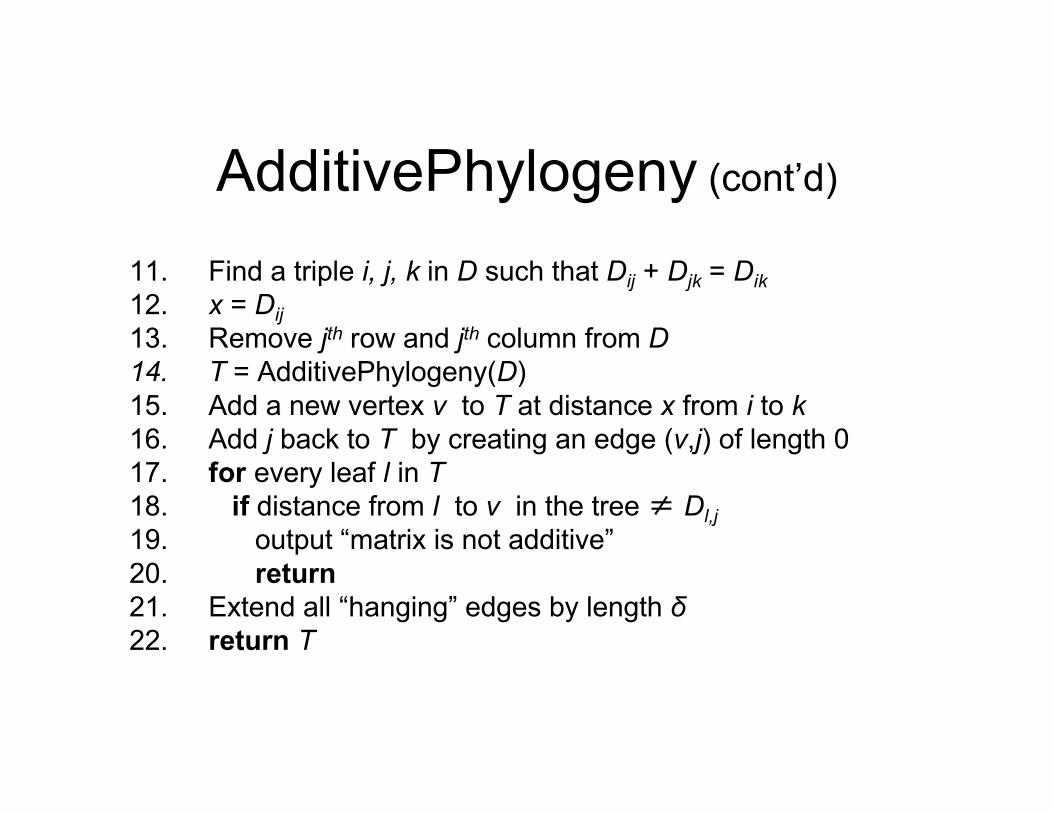
11. Find a triple i, j, k in D such that Dij + Djk = Dik12. x = Dij13. Remove jth row and jth column from D14. T = AdditivePhylogeny(D)15. Add a new vertex v to T at distance x from i to k16. Add j back to T by creating an edge (v,j) of length 017. for every leaf l in T18. if distance from l to v in the tree ≠ Dl,j19. output “matrix is not additive”20. return21. Extend all “hanging” edges by length δ22. return T

AdditivePhylogeny (Cont’d)

• This algorithm checks if the matrix D isadditive, and if so, returns the tree T.

• How to compute the trimmingparameter δ ?

• Inefficient way to check additivity• More efficient way comes from “Four

point condition”

The Four Point Condition

• Another additivity check is the “four-point condition”

• Let 1 ≤ i,j,k,l ≤ n be four distinct leavesin a tree

The Four Point Condition (cont’d)

Compute: 1. Dij + Dkl, 2. Dik + Djl, 3. Dil + Djk

1

2 32 and 3 representthe samenumber: thelength of alledges + themiddle edge (it iscounted twice)

1 represents asmallernumber: thelength of alledges – themiddle edge

The Four Point Condition:Theorem

• The four point condition for the quarteti,j,k,l is satisfied if two of these sumsare the same, with the third sum smallerthan these first two

• Theorem : An n x n matrix D is additiveif and only if the four point conditionholds for every quartet 1 ≤ i,j,k,l ≤ n

Solution 2

UPGMA: Unweighted Pair GroupMethod with Arithmetic Mean

• UPGMA is a clustering algorithm that:– computes the distance between clusters

using average pairwise distance– assigns a height to every vertex in the

tree

Clustering in UPGMA• Given two disjoint clusters Ci, Cj of

sequences, 1 dij = ––––––––– Σ{p ∈Ci, q ∈Cj}dpq

|Ci| × |Cj|

• Algorithm is a variant of the hierarchicalclustering algorithm

UPGMA AlgorithmInitialization:

Assign each xi to its own cluster CiDefine one leaf per sequence, each at height 0

Iteration:Find two clusters Ci and Cj such that dij is minLet Ck = Ci ∪ CjAdd a vertex connecting Ci, Cj and place it at height dij /2

Length of edge (Ci,Ck) = h(Ck) - h(Ci) Length of edge (Cj,Ck) = h(Ck) - h(Cj)

Delete clusters Ci and CjTermination:

When a single cluster remains

UPGMA Algorithm (cont’d)

1 4

3 2 5

1 4 2 3 5

UPGMA’s Weakness

• The algorithm produces an ultrametric tree :the distance from the root to any leaf is thesame

• UPGMA assumes a constant molecular clock:all species represented by the leaves in thetree are assumed to accumulate mutations(and thus evolve) at the same rate. This is amajor pitfall of UPGMA.

UPGMA’s Weakness:Example

2

3

41 1 4 32

Correct treeUPGMA

Solution 3

Using Neighboring Leaves to Construct the Tree

• Find neighboring leaves i and j with parent k• Remove the rows and columns of i and j• Add a new row and column corresponding to k, where

the distance from k to any other leaf m can becomputed as:

Dkm = (Dim + Djm – Dij)/2

Compress i and j intok, iterate algorithm forrest of tree

Finding Neighboring Leaves• To find neighboring leaves we simply select

a pair of closest leaves.• WRONG !

Finding Neighboring Leaves• Closest leaves aren’t necessarily neighbors• i and j are neighbors, but (dij = 13) > (djk =

12)

• Finding a pair of neighboring leaves is a nontrivial problem!

Neighbor Joining Algorithm

• In 1987 Naruya Saitou and Masatoshi Neideveloped a neighbor joining algorithm forphylogenetic tree reconstruction

• Finds a pair of leaves that are close toeach other but far from other leaves:implicitly finds a pair of neighboring leaves

Solution 4

Alignment Matrix vs. Distance Matrix

Sequence a gene of length mnucleotides in n species to generate a n x m alignment matrix

n x n distancematrix

CANNOT betransformed backinto alignmentmatrix becauseinformation waslost on the forwardtransformation

Transforminto…

Character-Based TreeReconstruction

• Better technique:– Character-based reconstruction algorithms

use the n x m alignment matrix (n = # species, m = #characters) directly instead of using distance matrix.– GOAL: determine what character strings at

internal nodes would best explain the characterstrings for the n observed species

Character-Based TreeReconstruction (cont’d)

• Characters may be nucleotides, where A, G,C, T are states of this character. Othercharacters may be the # of eyes or legs or theshape of a beak or a fin.

• By setting the length of an edge in the tree tothe Hamming distance, we may define theparsimony score of the tree as the sum ofthe lengths (weights) of the edges

Parsimony Approach toEvolutionary Tree Reconstruction

• Applies Occam’s razor principle to identifythe simplest explanation for the data

• Assumes observed character differencesresulted from the fewest possiblemutations

• Seeks the tree that yields lowest possibleparsimony score - sum of cost of allmutations found in the tree

Parsimony and TreeReconstruction

Small Parsimony Problem

• Input: Tree T with each leaf labeled by an m-character string.

• Output: Labeling of internal vertices of thetree T minimizing the parsimony score.

• We can assume that every leaf is labeled bya single character, because the characters inthe string are independent.

Weighted Small Parsimony Problem• A more general version of Small Parsimony

Problem• Input includes a k * k scoring matrix describing the

cost of transformation of each of k states intoanother one

• For Small Parsimony problem, the scoring matrix isbased on Hamming distance

dH(v, w) = 0 if v=w dH(v, w) = 1 otherwise

Scoring Matrices

0111C1011G1101T1110ACGTA

0449C4024G4203T9430ACGTA

Small Parsimony Problem Weighted Parsimony Problem

Weighted Small ParsimonyProblem: Formulation

• Input: Tree T with each leaf labeled byelements of a k-letter alphabet and a k x kscoring matrix (δij)

• Output: Labeling of internal vertices of thetree T minimizing the weighted parsimonyscore

Sankoff’s Algorithm

• Check children’severy vertex anddetermine theminimum betweenthem

• An example

Sankoff Algorithm: DynamicProgramming

• Calculate and keep track of a score forevery possible label at each vertex– st(v) = minimum parsimony score of the

subtree rooted at vertex v if v has character t• The score at each vertex is based on

scores of its children:– st(parent) = mini {si( left child ) + δi, t} + minj {sj( right child ) + δj, t}

Sankoff Algorithm (cont.)

• Begin at leaves:– If leaf has the character in question, score

is 0– Else, score is ∞


st(v) = mini {si(u) + δi, t} +minj{sj(w) + δj, t}

sA(v) = mini{si(u) + δi, A}+ minj{sj(w) + δj, A}

∞9∞C

∞4∞G

∞3∞T

000A

sumδi, Asi(u)

sA(v) = 0



sA(v) = mini{si(u) + δi, A}+ minj{sj(w) + δj, A}

990C

∞4∞G

∞3∞T

∞0∞A

sumδj, Asj(u)

+ 9 = 9sA(v) = 0



Repeat for T, G, and C


Repeat for right subtree


Repeat for root


Smallest score at root is minimum weightedparsimony score In this case, 9 –

so label with T

Sankoff Algorithm: Travelingdown the Tree

• The scores at the root vertex have beencomputed by going up the tree

• After the scores at root vertex arecomputed the Sankoff algorithm movesdown the tree and assign each vertex withoptimal character.


9 is derived from 7 + 2

So left child is T,

And right child is T


And the tree is thus labeled…

Large Parsimony Problem

• Input: An n x m matrix M describing nspecies, each represented by an m-characterstring

• Output: A tree T with n leaves labeled by then rows of matrix M, and a labeling of theinternal vertices such that the parsimonyscore is minimized over all possible trees andall possible labelings of internal vertices

Large Parsimony Problem(cont.)

• Possible search space is huge, especially asn increases– (2n – 3)!! possible rooted trees– (2n – 5)!! possible unrooted trees

• Problem is NP-complete– Exhaustive search only possible w/ small n(< 10)

• Hence, branch and bound or heuristics used

Nearest Neighbor InterchangeA Greedy Algorithm

• A Branch Swapping algorithm• Only evaluates a subset of all possible trees• Defines a neighbor of a tree as one reachable

by a nearest neighbor interchange– A rearrangement of the four subtrees defined by

one internal edge– Only three different arrangements per edge

evolutionary tree reconstruction (chapter...

Documents