evolutionary software architecture design · evolutionary software architecture ......
TRANSCRIPT

Outi Räihä
Evolutionary Software Architecture
Design
DEPARTMENT OF COMPUTER SCIENCES UNIVERSITY OF TAMPERE
D‐2008‐11
TAMPERE 2008

UNIVERSITY OF TAMPERE DEPARTMENT OF COMPUTER SCIENCES SERIES OF PUBLICATIONS D – NET PUBLICATIONS D‐2008‐11, SEPTEMBER 2008
Outi Räihä
Evolutionary Software Architecture
Design DEPARTMENT OF COMPUTER SCIENCES FIN‐33014 UNIVERSITY OF TAMPERE ISBN 978‐951‐44‐7505‐4 ISSN 1795‐4274

Abstract
This thesis experiments with a novel approach to applying genetic algorithms in softwarearchitecture design by giving the structure of an architecture at a highly abstract level.Previously in the literature, genetic algorithms are used only to improve existingarchitectures. The structure and evaluation of software architectures and the principlesof metaheuristic search algorithms are introduced to give a basis to understand theimplementation. Current research in the field of searchbased software engineering isexplored to give a perspective to the implementation presented in this thesis. The chosengenetic construction of software architectures is based on a model which containsinformation of a set of responsibilities and dependencies between them. Animplementation using this model is presented, as well as test results achieved from a casestudy made on a sketch of an electronic home control system. The test results show thatquality results can be achieved using the selected approach and that the presentedimplementation is a good starting point for future research.
Key words and terms: searchbased software engineering, genetic algorithms, softwarearchitecture, software design

Contents1. Introduction ...........................................................................................................12. Software architectures ............................................................................................3
2.1. The structure of an architecture .....................................................................32.2. Standard solutions .........................................................................................5
2.2.1. Design patterns ..................................................................................52.2.2. Architecture styles..............................................................................7
2.3. Evaluating an architecture .............................................................................92.3.1. Evaluation using metrics.....................................................................92.3.2. Evaluation using human expertise.....................................................14
3. Metaheuristic search algorithms...........................................................................163.1. Genetic algorithms.......................................................................................16
3.1.1. Encoding..........................................................................................173.1.2. Mutations.........................................................................................183.1.3. Crossover ........................................................................................183.1.4. Fitness function................................................................................203.1.5. Selection operator ............................................................................203.1.6. Executing a genetic algorithm ..........................................................21
3.2. Tabu search and simulated annealing ...........................................................233.2.1. Tabu search......................................................................................233.2.2. Simulated annealing .........................................................................24
4. Search algorithms in software engineering ............................................................264.1. Search algorithms in software design ...........................................................26
4.1.1. Software clustering ..........................................................................264.1.2. Systems integration ..........................................................................304.1.3. Systems refactoring..........................................................................314.1.4. Architecture development ................................................................34
4.2. Search algorithms in software analysis and testing........................................375. Genetic construction of software architectures......................................................40
5.1. Architecture representation..........................................................................405.2. Mutations....................................................................................................415.3. Crossover....................................................................................................445.4. Architecture laws ........................................................................................47
6. Implementation.....................................................................................................496.1. Presenting the program................................................................................49
6.1.1. Structure..........................................................................................496.1.2. Algorithms.......................................................................................52

6.1.3. Parameters .......................................................................................596.2. Evaluation metrics.......................................................................................60
6.2.1. Efficiency.........................................................................................616.2.2. Modifiability.....................................................................................62
7. Experiments .........................................................................................................647.1. Fitness development ....................................................................................647.2. Example solutions .......................................................................................697.3. Remarks on adjusting the parameters...........................................................76
8. Conclusions..........................................................................................................788.1. Presenting the results...................................................................................788.2. Success evaluation.......................................................................................798.3. Future work ................................................................................................80
References ................................................................................................................ 82
AppendicesAppendix A: Case study dataAppendix B: Fitness study parametersAppendix C: Example solutions’ parameters

1
1. IntroductionThe most constant thing in the field of software engineering today is that the field ischanging. Software systems become larger and more complex, while at the same timethe mobile industry is growing rapidly, calling for new techniques and intricate systemsto be implemented with limited resources. As software enterprises become multinational,the need for shared systems also grows. As the systems grow in complexity, so does theneed for highly talented software architects to keep the systems under control, which isnot an easy task especially when thinking of dynamic systems with constantly changingarchitectures. Clearly, some kind of automated method is needed in order to aid thedesign of such dynamic architectures by giving the human architects suggestions andstarting points which they can then finetune into quality software architectures.
What could such a method be? What can be used to evolve modifiable, reusable andefficient software architectures from complicated sets of requirements, especially if thearchitectures need to conform to changes in their environments? A precedent to thisproblem can be found in nature, where complex species have evolved from simpleorganisms, and are constantly able to adapt to changes in the environment. The evolutionhappens through generations with the idea of the survival of the fittest: the ones with theability to survive will be able to produce new offspring who will then inherit theproperties needed for survival. Changes in species also occur through mutations, whichare the key to survival when the change in environment is so drastic that rapid adaptationis needed, but happen also constantly at a lower level. However, the adaptation “project”with species takes perhaps hundreds of generations and years, which is not acceptable inthe field of software engineering. Fortunately, a simulation can be done quite fast toachieve similar results with the use of genetic algorithms.
Genetic algorithms operate with analogies to evolution in biology. As in biology achromosome keeps the “solution” to the question as to how certain properties of aspecies work, a solution to a software engineering problem can be modeled as a“chromosome” in order for it to be operated by a genetic algorithm. This model is thenaltered by mutations, which change one specific feature, and crossovers which, as innature, combine the characteristics of two individuals in their offspring.
Genetic algorithms are suitable for modifying software architectures as they too havecertain constants which can be implemented in various ways. An architecture is based onthe requirements as to what the software system is supposed to do. The basicarchitecture deals with the question of how the operations related to the requirementsare divided into components. When further developing architectures, mechanisms suchas interfaces and inheritance can also be added to the design. Thus, the set ofrequirements and their positioning in the system represents the basic individual, whichthen evolves as positions of requirements are changed and mechanisms are added. As

2
there is theoretically an exponential amount of possible designs for a system, the use ofgenetic algorithms to solve the problem is justified.
The common feature with all the current research activities on applying searchalgorithms to architecture design is that a reasonably good architecture is needed as astarting point, and the search algorithm merely attempts to improve this architecture withrespective to some quality metrics. This means that considerable effort is needed beforethe algorithm can be executed, and as the base solution can be assumed as a standardone, this also somewhat limits the possible solutions the algorithm can reach. Thisrestriction decreases the innovativeness of the method: if given the algorithm “freehands”, it might be able to reach solutions that a human designer might not find at all,but still have a high quality. Thus, an approach that only needs the basic requirements(responsibilities) of the system would both save the initial work and give the algorithm achance for a more thorough traverse through the possible solutions.
In my thesis, I have further developed the approach of starting only with a set ofresponsibilities: this approach was first introduced in my Master’s thesis [Räihä, 2008]. Ihave derived a responsibility dependency graph which is then given as input to a geneticalgorithm, which will produce a suggestion for the architecture of the given system as aUML class diagram. I begin my thesis by presenting the structure and current evaluationmethods of software architectures in Chapter 2. In Chapter 3 I describe metaheuristicsearch algorithms, and especially give a thorough presentation of genetic algorithms. Thecurrent research involved with the application of metaheuristic search algorithms insoftware engineering is surveyed in Chapter 4. In Chapters 5 and 6 I present myimplementation, first from a logical point of view, as to how an architecture can bemodeled for a genetic algorithm, and then from a practical view by giving a detaileddescription of the implementation and the evaluation metrics used. Results from testswhere the implemented algorithm was used on a model of an electronic home controlsystem are presented in Chapter 7, and in Chapter 8 I present the outcome of this thesisand my concluding remarks.

3
2. Software architecturesSoftware architecture is defined by the IEEE Standard 14712000 [IEEE, 2000] as “thefundamental organization of a system embodied in its components, their relationships toeach other and to the environment, and the principles guiding its design and evolution”.Thus, software architecture defines the general structure of the software. An architectureshould always be described or modeled somehow, otherwise it does not exist. In reverseengineering one tries to detect the architecture of software from the source code bylooking at what kind of packages it has, and by generating class diagrams from the code.Normally, the architecture of software is designed before the actual implementation, as itis possible to efficiently evaluate the architecture, and thus point out possible weaknessesof the software before beginning the implementation.
The structure of architecture and the evaluation metrics presented in this chapter willbe used in Chapter 5, where I present how architectures can be modeled in order tomanipulate them with a genetic algorithm, and in Chapter 6, where I discuss theevaluation methods used in the implementation. The studies surveyed in Chapter 4 alsouse many of the metrics presented here as well as concepts concerning architecturalquality.
2.1. The structure of an architectureAs stated, software architecture describes the components of a software and therelationships between these components. We must now consider what can be thought ofas a component, and what as a relationship.
A software component is defined as an individual and independent software unit thatoffers its services through welldefined interfaces [Koskimies ja Mikkonen, 2005]. Thisdefinition requires that the topics of dependency, usage and size are also dealt with.Firstly, a component should never be completely dependent of another component. Acomponent can, however, be dependent on services that are provided by some othercomponents, thus requiring an interface to those components. Secondly, a componentcan be taken to use as a single unit with no regard to other software units if thecomponent is still provided the services it needs. Thirdly, there are no generalrestrictions to the size of a component. A component can be extremely small, providingonly a few simple services, or it can contain a whole application. If the component isvery big and forms a significant subsystem within itself, it may be in order to describethe architecture of that single component, although normally an architecture descriptiondoes not consider what the components entail [Koskimies ja Mikkonen, 2005].
When thinking of objectoriented design, the basic component provides some kind offunctionality to the system and consists of classes. Classes can be defined as abstract andthey can be inherited from each other. Classes interact with one another by either

4
straightforwardly calling operations from other classes or through interfaces. Thesimplest component may only include one class. Because of this close relationshipbetween components and classes, architectures are often described with UML classdiagrams. Other components that are often present in the system, but do not providemuch functionality, are components such as databases, hardware drivers and messagedispatchers.
One of the key points in software engineering is to separate what one wants toaccomplish (the functionality provided by components) and how to accomplish it. This isapplied to software components in such a way that the implementation of a service that acomponent provides should be separated from the abstraction of the service:components should not be directly dependent on one another, but on the abstraction ofthe service that the component provides [Koskimies ja Mikkonen, 2005]. Theabstraction is presented as an interface that provides access to services to thecomponents that require the services in question. This corresponds to the idea thatinterfaces may be either provided or required.
Interfaces include all the information about a service: the service’s name, itsparameters and their types and the type of the possible result [Koskimies ja Mikkonen,2005]. Interfaces have developed from abstract classes into their own program units.Abstract classes and interfaces are still interlinked; by inheriting several concrete classesfrom an abstract class one can thus give several implementations to one interface[Koskimies ja Mikkonen, 2005]. One component or class can also implement severalinterfaces.
There are several ways for components to interact with one another. Most of thesemethods are finetuned ways of how interfaces are used in order to consider the needs ofa specific type of application. I will briefly present these communication methods, as forthe purpose of this thesis, it is more important to be aware that such methods exist andpossibly recognize them from an architecture design than to know all the ins and outs ofthese communication methods and to able to actively implement them. I will describe themethods as they are presented by Koskimies and Mikkonen [2005].
Firstly, the interfaces a component provides may be divided into more detailed roleinterfaces, each roleinterface responding to the special need of the component requiringthat interface, instead of keeping all the services of the providing component in one biginterface. Secondly, when addressed with the problem of multiple components usingeach other and thus creating a complex net of dependencies, one can use a mediator tohandle the interaction between the components. Thus, all the components only dependon this one mediator, which is often a specialized interface. Thirdly, an even morepowerful method than the basic interface is forwarding. This means that the componentreceiving a request for a service does not provide that service itself, but forwards therequest to another component, which then acts on it. Fourthly, the interaction between

5
components can be based on events. We can now think that asking for a service is theevent itself, and providing a service is reacting to the event. The component creating theevent is now the source and the component reacting to it is the observer. In this caseboth components are providing and requesting an interface to communicate with eachother: the source component provides an interface through which the observer canregister as a service provider, and the observer provides an interface through which itsservices can be provided.
I end this section with a brief summary. An architecture is based on the idea ofcomponents and the relationships between them. Components provide services that othercomponents may need. This results in a dependency between components which isideally handled with interfaces: the component needing a service requires an interface,which the component offering the service then provides by implementing that interface.How the interface is built, i.e. what kind of communication method is used, depends onthe application and its requirements.
2.2. Standard solutionsWhen designing an architecture, there are some commonly used architecture styles anddesign patterns that can be used as general guidelines for the architecture. These stylesand guidelines all have their positive and negative aspects, so one should think what themain problems in the system are, and then study the implementation of styles and designpatterns that are generally known to solve those problems. One does not necessarilyneed to categorize an architecture as a set of the known styles or patterns, but if it can becategorized, it usually indicates good structure in the architecture.
2.2.1. Design patternsA design pattern is used to solve a particular problem in the architecture. Designpatterns often appear in several parts of an architecture, and one architecture can containseveral different patterns. The list of design patterns made by Gamma et al. [1995] isrecognized as the current standard in design pattern classification. This list contains over20 patterns, which can be divided into creational patterns, structural patterns andbehavioral patterns. For the purpose of this thesis it is not necessary to introduce themall, and thus only a few of the most common or relevant patterns are described in moredetail.
Firstly, from the category of creational patterns, there are the factory method and theabstract factory method, which are common design patterns when one has a lot ofcomponents that work together or have a similar purpose. When applying the abstractfactory method, an interface should be provided for creating families of related ordependent objects without actually specifying their concrete classes [Gamma et al.,1995]. This means that two or more concrete classes that are responsible for similarobjects will implement the same interface, through which these families of objects can be

6
dealt with. In the factory method an interface is also used for creating an object, butdeciding the class that the object represents is left to subclasses [Gamma et al., 1995].This means that the objects of a certain family all inherit the “baseobject” of that familyin order to ensure that they contain the required properties.
These design methods are presented together as they are closely linked: abstractfactory classes are commonly implemented with factory methods. Although the abstractfactory method and the factory method are very commonly used in current architecturedesign, I can imagine that automatically producing an architecture where such a patterncould be found is a great challenge. These design patterns rely on the recognition ofsimilarities between objects and the ability to group objects by some standards.However, similarities between objects are difficult to express formally, but are rathersomething that experts can simply see. Thus, to train an algorithm to find such abstractsimilarities will definitely need finetuned definitions of the objects and relationspresented to the algorithm.
Secondly, there is the composite method, which is a structural pattern, in whichobjects are composed into tree structures to represent partwhole hierarchies. Acomposite also allows clients treat individual objects and compositions of objectsuniformly [Gamma et al., 1995]. The composite pattern defines hierarchies consisting ofprimitive objects and composite objects. Primitive objects can form composite objects,which in turn can form more complex composite objects, and so on recursively [Gammaet al., 1995]. Vice versa, all composite objects can be broken down to primitive objects.The composite method goes well with the responsibility based approach used in thisthesis, as all responsibilities can be thought of as primitive objects or services, whichform composites that other composites use.
Thirdly, there is the Façade pattern, which has implemented in this work, and istherefore especially interesting. The Façade is a structural pattern, and its intention is toprovide a unified interface to a set of interfaces in a subsystem [Gamma et al., 1995].This will make the subsystem easier to use through the higherlevel interface defined bythe Façade. Structuring a system into subsystems reduces complexity, and a commondesign goal is to minimize dependencies between the defined subsystems [Gamma et al.,1995]. A façade can aid in achieving this goal, and its proper placement can beeffectively measured by metrics dealing with complexity and the number of connectionsbetween classes.
Finally, I present the Strategy pattern, which has also been implemented. TheStrategy pattern is a behavioral pattern, which encapsulates an algorithm, thus making itinterchangeable and independent of the using client. A Strategy pattern can be applied,e.g., when different variants of an algorithm need to be defined or there are severalrelated classes that only differ in their behavior [Gamma et al., 1995]. From theperspective of responsibilities, a strategy can be seen as wellplaced if the responsibility

7
is highly variable. For example, measuring the position of drapes can be executed withdifferent algorithms that have the same outcome. In this case, a Strategy pattern wouldvery well fit in the system.
As automating the design of an architecture mainly deals with the structure of anarchitecture, structural patterns are logically the ones that are most likely to be foundfrom the resulting architecture. Thus, structural patterns are the most interesting patterngroup from the viewpoint of this thesis. Overall, structural patterns deal with howclasses and objects are composed to form larger structures. Structural class patternscommonly solve problems with clever inheritance to achieve interfaces forimplementations, and structural object patterns describe how objects can be composed toachieve new functionalities [Gamma et al., 1995]. Other structural design patternsbesides the composite pattern are, for example, the adapter pattern. In this pattern, anincompatible interface is converted to let such classes work together that could notbefore because of the “wrong” type of the provided interface. Another example is thebridge pattern, which builds a “bridge” between an abstraction and its implementation,so they can vary independently [Gamma et al., 1995].
2.2.2. Architecture stylesArchitecture styles have the same purpose as design patterns: they are used to solve aproblem in the design of the architecture. It is often difficult to make a differencebetween design patterns and architectural styles, but the general guideline is that whiledesign patterns are used at a particular subsystem in the architecture, architecture stylessolve a problem regarding the whole architecture [Koskimies ja Mikkonen, 2005]. Aswith design patterns, it is not necessary to go through all possible architecture styles, soonly the most interesting ones from this thesis’ point of view are described with moredetail.
Firstly, I present the layered architecture. A layered architecture is composed oflevels that have been organized into an ascending order by some principle of abstraction[Koskimies ja Mikkonen, 2005]. This is usually done so that the parts of the system thatare closer to the user have a lower level of abstraction than the parts that are closer tothe application. Because the levels of abstraction can often be hard to identify, the levelsor layers in the architecture are deduced by how different components use services fromother components. A higher level in the architecture uses services from a lower level[Koskimies ja Mikkonen, 2005]. However, layered architectures are rarely sostraightforward. It is quite common that a layer is simply passed in a service call, and, forexample, a service is required at the fifth level that is provided at the third level. It is alsopossible that a lower layer needs to call a service from an upper layer. This is, however,a sign of a serious problem in the architecture. Layered architectures are very common,and can be used in almost any system [Koskimies ja Mikkonen, 2005]. The layeredarchitecture model encourages a minimized design in terms of dependencies, for in the

8
ideal case, any layer only depends on layers below itself. This kind of architecture modelis also very easy to understand, as it divides the system to subsections at a high level[Koskimies ja Mikkonen, 2005]. The layered architecture is something that is veryinteresting from my viewpoint and that of thinking through responsibilities. When havinga network of responsibilities, we can quite simply begin forming layers by placing theresponsibilities that do not depend from any other responsibilities at the bottom layer,and going on until at the top level are the responsibilities that have a very longdependency path behind them.
Secondly, there is the pipes and filters architectural style. It consists of processingunits (filters) and the connections (pipes) between them that carry the information thatneeds to be processed. The role of pipes is to passively transport data which the filterswill actively process. The pipes and filters architecture is good for the kind of systemwhere the purpose is to mainly develop and process a common dataflow [Koskimies jaMikkonen, 2005]. To implement the pipes and filters architecture it requires that eachprocessing unit can be implemented independently: a unit can not depend on any of theother processing units, and must only be able to understand the data that is brought to itto process. The simplest form of a pipes and filters architecture is a pipeline architecture,where the data moves straightforwardly from one processing unit to another along astraight “conveyer belt”. There are two ways in operating this “conveyer belt”, to pushor pull. If we choose to push, then the unit that first generates the data will push it to thesecond unit for processing, which will then continue to push to the next processing unitand so on, until the data reaches the final unit needing the “end product”, i.e. thecompletely processed data unit. If we choose to pull the data, then the final unit needingthe data will “pull” data from the processing unit preceding it, which will then call for thedata from its preceding unit, and so on [Koskimies ja Mikkonen, 2005]. A pipes andfilters architecture can be useful from this thesis’s viewpoint if the responsibilities wework with all deal with the same kind of data, and merely have more finetunedresponsibilities regarding that data, or if they can be arranged in quite a straightforwardline, i.e., if the dependency graph does not have any cycles and a unique ending point canbe identified.
Finally, an architecture style especially used in this thesis is the message dispatcherarchitecture, where a group of components communicate with each other through acentered message dispatcher. All the components have a common interface that containsall the operations that are needed in order to send and receive messages to and from thedispatcher [Koskimies ja Mikkonen, 2005]. It is important to notice that now thecomponents only communicate with the dispatcher: although they send and receivemessages to and from other components, no component can actually “see” the message’spath past the dispatcher. Thus, no component actually knows where its messages willend up or where the messages it has received originate from. A message dispatcher

9
architecture suits well in a situation where the system has a large number of componentsthat need to communicate with each other, but there is not much information of thequality or quantity of the messages sent between components [Koskimies ja Mikkonen,2005]. A message dispatcher architecture is defined by the set of componentscommunicating with each other, the messages with which the components communicate,the operations with which components react to messages, the rules with which thecomponents and messages are registered to the system, the rules on how the dispatcherforwards messages to components and the model of concurrency [Koskimies jaMikkonen, 2005].
Other common architecture styles are service oriented architectures, such as theclientserver architecture, where client components ask for the services they need fromthe server components. Clientserver architecture is often thought as a distributedsystem. Other, more specialized architecture styles are for example the modelviewcontroller architecture or the interpreter architecture.
2.3. Evaluating an architectureWhen evaluating a software architecture we must keep in mind that the architectureunder evaluation is, roughly stated, merely a picture of how the different components areplaced in the system and how they depend from one another. Thus, there is no absolutemethod for evaluating an architecture; just as there is no absolute answer to the questionhow good exactly a particular architecture is. Currently there are two kinds of methodsfor software architecture evaluation. Firstly, there are metrics that can be used when oneknows the software in detail. These metrics often calculate the cohesion and couplingbetween classes, so it must be known what kind of operations the classes include, andhow they are linked to each other. Secondly, there are methods to evaluate thearchitecture by the means of using the expertise of software engineers, going throughmeetings and several iterations when the architecture is broken down to pieces and theanalysts attempt to identify all the possible risks that can be related to the suggestedsolution.
Whatever method is used to evaluate architecture, one thing must be kept in mind:no architecture can be evaluated from an overall point of view. There are differentviewpoints or quality attributes for an architecture, such as efficiency or performance,maintainability, reliability, security, movability, usability, availability, reusability andmodifiability [Koskimies ja Mikkonen, 2005]. The actual evaluation of an architecture isthe sum of evaluations of a combination of these viewpoints, and it is of course mostpreferred if as many relevant viewpoints as possible have been considered.
2.3.1. Evaluation using metricsEvaluating a software architecture using some kind of metrics system is often based onthe assumption that we are dealing with objectoriented design. Thus, metrics can be

10
used for different kinds of calculations of dependencies between and within classes,which can give guidelines on how good a structure the architecture in question has.Rosenberg and Hyatt [1997] define five different qualities that can be measured bymetrics for objectoriented design: efficiency, complexity, understandability, reusability,and testability/maintainability. I will now introduce some metrics suites and definitionsthat can be used when evaluating objectoriented designs.
The metrics suite by Chidamber and Kemerer [1994] is based on four principles thatrule objectoriented design process: identification of classes (and objects), identificationof semantics of classes (and objects), identification of relationships between classes (andobjects) and implementation of classes (and objects). Based on these principles,Chidamber and Kemerer [1994] present a metrics suite that consists of six differentmetrics: weighted methods per class (WMC), depth of inheritance tree (DIT), numberof children (NOC), coupling between object classes (CBO), response for a class (RFC),and lack of cohesion in methods (LCOM).
The WMC metric is defined as the sum of complexities of the methods within aclass. If all methods are equally complex, this is simply the amount of methods in a class.It predicts how much time and effort is required to develop and maintain the class, howmuch the children of the class are impacted by the class and how general the class is[Chidamber and Kemerer, 1994]. These aspects relate to quality attributes such asmaintainability and reusability. Rosenberg and Hyatt [1997] point out that WMC alsoindicates understandability.
DIT is selfdefined as it is the length from a class node to the root of the inheritancetree where the node is. If the class does not inherit any class, then DIT is zero. Thedeeper a class is in a hierarchy, the harder it is to predict its behavior, the more complexthe design will most likely become, and the greater the potential reuse for inheritedmethods [Chidamber and Kemerer, 1994]. Thus, DIT predicts negative aspects ofcomplexity and maintainability but a positive aspect of reusability. According toRosenberg and Hyatt [1997], DIT primarily evaluates efficiency and reusability, but canalso be used as an indicator for understandability and testability.
NOC is as clear as DIT as it calculates how many classes inherit the class inquestion. It also predicts good reusability, but a high value warns of improperabstractions of the parent class and indicates that a good deal of testing should be doneto the methods of the class [Chidamber and Kemerer, 1994]. In addition to testability,NOC evaluates efficiency and reusability [Rosenberg and Hyatt, 1997].
CBO is defined as the number of classes to which the class in question is coupled,i.e., CBO for class A is |B| + |C|, where B is the set of classes that class A depends on,and C is the set of classes that depend on class A (where |X| stands for the cardinality ofX). A high CBO value indicates poor reusability, modularity and maintainability, and is

11
usually a sign of need for excessive testing [Chidamber and Kemerer, 1994]. CBO canalso be used as an evaluator for efficiency [Rosenberg and Hyatt, 1997].
RFC is defined as the size of the response set (RS) for the class, when the RS is theunion of the set of all methods in the class and the set of methods called by the methodsin the class. RFC contributes mainly in bringing out testing issues, but it also indicatescomplexity [Chidamber and Kemerer, 1994]. According to Rosenberg and Hyatt [1997],RFC evaluates understandability, maintainability and testability.
Finally, LCOM measures in what extend methods within the same class use the sameinstance variables. LCOM is a count of method pairs with a similarity of zero, i.e., theyhave no instance variables in common, minus the count of method pairs with a similaritythat is not zero. Cohesiveness is very desirable, as it promotes encapsulation; classeswith low cohesion should most probably be divided into two or more subclasses, andlow cohesion also indicates high complexity [Chidamber and Kemerer, 1994]. Inaddition, LCOM evaluates efficiency and reusability [Rosenberg and Hyatt, 1997].
In addition to the metrics by Chidamber and Kemerer, Rosenberg and Hyatt [1997]present two additional metrics for evaluation at the method level, cyclomatic complexity(CC) and size. CC is used to evaluate the complexity of an algorithm in a method. Quitelogically, CC measures mainly complexity, but is also related to all the other qualityattributes. The size of a method can be measured by several ways, e.g., by lines of codeor the number of statements. It evaluates mainly understandability, reusability andmaintainability.
A popular metric when dealing with the software or module clustering problem is themodularization quality (MQ). There are several versions of this metric, but it is alwayssome kind of a combination of coupling and cohesion metrics, calculating the inter andintraconnectivities between and within clusters, respectively. A high MQ value indicateshigh cohesion and low coupling. One version of the MQ metric is presented by Doval etal. [1999], who begin by defining the intraconnectivity Ai of cluster i as
Ai = 2i
i
Nµ
,
where Ni is the number of components and µi is the number of relationships to and frommodules within the same cluster. Ai is 0 when no module is connected to another modulewithin the cluster, and 1 when each module in the cluster is connected to every modulein the same cluster. Interconnectivity Ei,j between clusters i and j, consisting of Ni and Nj
components, respectively, with ij relationships between the modules of both clusters, isdefined as
Ei,j = 0 , if i = j, and
Ei,j =ji
ij
NN2ε
,if i j
12
[Doval et al., 1999]. MQ is now a combination of these connectivity measures: when amodule dependency graph is partitioned into k clusters,
MQ = Ai , if k = 1, and
MQ =k
Ak
i i∑ =1
2)1(
1, ,
−∑ =
kkEk
ji ji , if k > 1.
The work by Doval et al. [1999] and the module clustering problem in which this metricis used, is presented in Chapter 4.
When defining what a software architecture is, the principles guiding its evolutionwere mentioned. Thus, it is natural that there should be metrics to evaluate the evolutionand refactoring of an architecture. Mens and Demeyer [2001] present such evolutionmetrics, the main metric being the distance between classes. This metric is very flexible,as the distance it measures depends on what is needed, i.e., how far two classes are fromeach other when considering, e.g., the number of methods, number of children or depthof inheritance tree. The distance between classes is defined so that, when p(x) is theproperty that is measured from class x, the distance between classes x and y is
dist(x; y) = 1 )()()()(
ypxpypxp
∪∩ .
Large distances between classes can indicate a complex system. Mens and Demeyer[2001] also discuss the emphasis of abstract methods and abstract classes in a system,and point out that all abstract classes should be base classes.
Sahraoui et al. [2000] present a list of inheritance and coupling metrics, where thesimplest metrics are NOC, CBO and number of methods (NOM), which is a simplerform of WMC, but the rest are more specialized extensions of the metrics presentedearlier. These include metrics such as classtoleaf depth (CLD), number of methodsoverridden (NMO), number of methods inherited (NMI), number of methods added(NMA), specialization index (SIX), data abstraction coupling (DAC’), informationflowbased inheritance coupling (IHICP), other classattribute import coupling(OCAIC), descendants methodmethod export coupling (DMMEC) and others methodmethod export coupling (OMMEC). By analyzing the results given by these metrics, thefollowing operations can be administered to the system: creating an abstract class,creating specialized subclasses and creating an aggregate class [Sahraoui et al., 2000].
Du Bois and Mens [2003] use a combination of the metrics defined above (numberof methods, CC, NOC, CBO, RFC and LCOM) in order to administrate a selection ofrefactoring operations (extracting a method, encapsulating a field and pulling up amethod) to a system. Thus, this suite of metrics can be used to both evaluate theexisting system and to use those results to evolve a system. As can be seen, the metricssuite presented by Chidamber and Kemerer [1994] acts as a good base for evaluatingarchitectures and evolving new metrics by using their six metrics as a starting point.

13
Another way of measuring is related to the stable/instable and abstract/concretelevels of the system, which is used by Amoui et al. [2006]; this is based on simplycounting the number of certain types of classes and dependencies.
Losavio et al. [2004] present ISO quality standards for measuring architectures.This model is somewhere in between pure metrics and evaluation using human expertise,which is discussed further on. The ISO 91261 quality model’s characteristics arefunctionality, reliability, usability, efficiency, maintainability and portability [Losavio etal., 2004] – a list quite similar to the one presented by Rosenberg and Hyatt [1997]. Inthe ISO model, the characteristics of quality are refined into subcharacteristics, whichare again refined to attributes, which are measured by metrics. Thus, the model needshuman expertise in making the refinements, but the end result is a measurable valuerelated to the architecture. As the characteristics have from three to five separatelymeasured subcharacteristics each, it is not practical to go through them all in the scopeof this paper. The most interesting quality measures being efficiency and maintainability,I will now present some example metrics for measuring the subcharacteristics of these.
Efficiency is divided into time behavior, resource behavior and compliance. Let usnow investigate how time behavior is measured. Time behavior means the capability ofthe software product to provide appropriate response time, processing time andthroughput rates under stated conditions [Losavio et al., 2004]. To measure this, onemust first identify all the components involved with functionality and the connectionsbetween them. The attribute is then computed as the sum of the time behaviors of thecomponents and the time behaviors of the connections. The time behavior of acomponent or a connection depends on the stimulus/event/functionality and the pathtaken in the architecture to respond to a stimulus for a given functionality [Losavio etal., 2004].
Maintainability is subcategorized into analyzability, changeability, stability,testability and compliance. Let us take changeability and stability as examples.Changeability is defined as the capability of the software to enable implementation ofmodifications, and stability is defined as the capability of the software to avoidunexpected effects from modifications of the software. In order to measure these (andtestability), two additional subcharacteristics need to be added to the ISO modelframework at architectural level: coupling and modularity [Losavio et al., 2004]. Thecomputations for changeability and stability need to be made for each couple ofconnected components on the number of incoming/outgoing messages, and for eachcomponent on the number of components depending on that component.
The examples of time behavior, changeability and stability are still something thatcan be seen as metrics: the resulting values are something that can be computed, albeitthat it might not be easy. However, there are many subcharacteristics in the ISO 91261quality model when the “counting rule” does not contain any calculation and thus, the
14
result is not numeral. For example, functionality contains subcharacteristics such asinteroperability and security, where the attribute that is to be “measured” is the presenceof a certain mechanism. Thus, to “count” the attribute, one needs to identify whether themechanism is present in the system [Losavio et al., 2004]. This is another point (inaddition to the redefining steps) where the ISO quality model can be seen as relyingmore on human expertise than being a set of metrics that can be used for automatedevaluation of an architecture.
2.3.2. Evaluation using human expertiseWhen evaluating an architecture there are three questions that should be answered in theevaluation. Firstly, is the designed architecture suitable for the system in question?Secondly, if there are several options to choose an architecture from, which is the bestfor the particular system and why? Thirdly, how good will different quality attributerequirements be? [Koskimies ja Mikkonen, 2005]
These questions alone demonstrate the difference between using metrics to givevalues to quality requirements and using human expertise: no metric can answer thequestion “why” when discussing the positive and negative points of differentarchitectural options. Metrics may also give very good values to individual qualityrequirements, but as a whole the architecture may not be at all suitable for the system inquestion. Hence, although metrics can aid in architecture evaluation and are basically theonly way of automated evaluation, they cannot replace the evaluation of experts.
The most widely used and known method for architecture evaluation is theArchitecture Tradeoff Analysis Method (ATAM) by Kazman et al. [2000]. Other knownarchitecture evaluation methods are the Maintenance Prediction Method by Jan Bosch,which concentrates in evaluating maintainability, and the Software Architecture AnalysisMethod developed in the Software Engineering Institute of CarnegieMellon University,which is mainly used for evaluating quality attributes that are related to modifiability[Koskimies ja Mikkonen, 2005]. As ATAM is the only method that can be used toevaluate all quality attributes, it is the one I will go into with more detail.
The main points of ATAM are to elicit and refine a precise statement of the keyquality attribute requirements concerning the architecture, to elicit and refine precisedesigning decisions for the architecture, and based on the two previous goals, toevaluate the architectural design decisions to determine if they fulfill the quality attributerequirements satisfactorily [Kazman et al., 2000]. The ATAM uses scenarios in order toanalyze whether the architecture fulfills all the necessary requirements and to see risksinvolved in the architecture. The ATAM proceeds in nine steps: presenting the methodfor the group of experts, presenting business drivers, presenting the architecture,identifying architecture approaches, generating quality attribute utility tree, analyzingarchitecture approaches, brainstorming and prioritizing scenarios, again analyzingarchitecture approaches, and finally presenting the results [Kazman et al., 2000]. The

15
steps where we can say that the architecture is evaluated as in how good it is in theATAM are when the quality attribute utility tree is generated, architecture approachesare analyzed and scenarios are brainstormed, so I will now concentrate on these steps.
When the architecture has been presented and the architecture styles have beenidentified, a quality attribute utility tree is generated. This is done by eliciting the qualityattributes that relate to the particular system and then breaking them down to the level ofscenarios, which are shown with stimuli and responses and prioritized [Kazman et al.,2000]. For each quality approach, the quality factor is divided into subfactors. Forexample, modifiability could be divided into GUImodifications and algorithmicmodifications. For each of these subfactors, detailed scenarios are described in order tosee how the subfactor in question affects the architecture [Kazman et al., 2000]. Forexample, GUImodifications may have a scenario that if a new feature is added to theapplication, the feature should be visible in the GUI within one day. These scenarios arethen prioritized according to how relevant they are to the system, how likely they are tohappen, and naturally, how critical they are for the quality attribute in question. Based onthe utility tree, experts can now concentrate on the high priority scenarios and analyzearchitectural approaches that satisfy these scenarios.
While the utility tree is manufactured by a smaller group of specialized architectureexperts, a scenario brainstorming session involves all the stakeholders involved in theproject. The purpose of this session is to gather all the possible ideas and scenarios thatrelate to the system and should be considered in the architecture [Kazman et al., 2000].
After the brainstorming of scenarios, all possible scenarios should be documentedeither as a result of the utility tree or the brainstorming sessions. The architecture expertsmay now reanalyze the architecture styles that have been documented and discussed, andperhaps even suggest a completely different solution if the brainstorming session broughtup many unexpected scenarios or the prioritizing of quality attributes was very differentfrom the one in the utility tree.
After all the steps of the ATAM, the outcomes of this method will include thearchitectural approaches documented, the set of scenarios and their prioritization, the setof attributebased questions, the utility tree, risks and sensitivity and tradeoff points inthe architecture [Kazman et al., 2000].
As can be seen, the ATAM relies purely on human expertise, and the evaluation ofarchitecture happens while the architecture is actually being developed. Some basicarchitectural approaches are first presented based on the known structure of the system,and as the quality attributes requirements of the system become clearer, the architectureundergoes several iterations of analysis, while the architecture is being refined anddifferent approaches may be considered. The “goodness” of the architecture can bedefined and measured by how well it satisfies the quality attribute requirements and how“easily” it responds to the scenarios related to the quality attributes.

16
3. Metaheuristic search algorithmsMany subproblems of several software engineering problems are known to be NPhard.For example software clustering, which is a special case of the general graph partitioningproblem, is NPhard. In such cases, nondeterministic search algorithms are useful, asthey are often capable of finding good enough solutions from a large search space. Thecharacteristics that enable such good results are that they do not need to go through allthe possible solutions; yet by being nondeterministic, it is possible to recover from asearch path that seemed good in the beginning, but resulted in a bad solution.
There are certain terms that are common to most search algorithms; theneighborhood and fitness of a solution. Each solution can be regarded as a point in thesearch space that needs to be explored. The neighborhood of a solution is the set of allavailable solutions that can be reached with one techniquespecific move from thecurrent solution. The concept of neighborhood is especially used in local searchalgorithms, such as hillclimbing, tabu search and simulated annealing. The fitness of asolution indicates how good the solution is. In rare cases, when the optimum is known,one tries to get the fitness value as close to the optimum as possible. Since this is hardlyever the case, it is usually attempted to maximize or minimize a fitness function.
For the purpose of this thesis, it is necessary to understand how search algorithmsoperate in order to understand the underlying concepts of the research presented inChapter 4, and the implementation presented in Chapters 5 and 6.
3.1. Genetic algorithmsGenetic algorithms were invented by John Holland in the 1960s. Holland’s original goalwas not to design application specific algorithms, but rather to formally study the waysof evolution and adaptation in nature and develop ways to import them into computerscience. Holland’s 1975 book Adaptation in Natural and Artificial Systems presents thegenetic algorithm as an abstraction of biological evolution and gives the theoreticalframework for adaptation under the genetic algorithm [Mitchell, 1994].
In order to explain genetic algorithms, some biological terminology needs to beclarified. All living organisms consist of cells, and every cell contains a set ofchromosomes, which are strings of DNA and give the basic information of the particularorganism. A chromosome can be further divided into genes, which in turn are functionalblocks of DNA, each gene representing some particular property of the organism. Thedifferent possibilities for each property, e.g. different colors of the eye, are called alleles.Each gene is located at a particular locus of the chromosome. When reproducing,crossover occurs: genes are exchanged between the pair of parent chromosomes. Theoffspring is subject to mutation, where single bits of DNA are changed. The fitness of anorganism is the probability that the organism will live to reproduce and carry on to thenext generation [Mitchell, 1996]. The set of individuals at hand at a given time is called apopulation.

17
Genetic algorithms are a way of using the ideas of evolution in computer science.When thinking of the evolution and development of species in nature, in order for thespecies to survive, it needs to meet the demands of its surroundings. Such evolution isachieved with mutations and crossovers between different individuals, while the fittestsurvive and are able to participate in creating the next generation.
In computer science, genetic algorithms are used to find a good solution from a verylarge solution set, the goal obviously being that the found solution is as good as possible.To operate with a genetic algorithm, one needs an encoding of the solution, an initialpopulation, mutation and crossover operators, a fitness function and a selection operatorfor choosing the survivors for the next generation.
3.1.1. EncodingAs stated, the basis of genetics in nature is a chromosome. When applying this thoughtto computer science and genetic algorithms, each individual in the search space, i.e. eachsolution to the problem at hand, needs to be encoded so that it can be thought of as achromosome. The most common and traditional way of doing this is to use a bit vector,i.e., a string of ones and zeros [Mitchell, 1996]. Thus every bit in the chromosomerepresents a gene in that locus, the alleles being one and zero. This has the advantage ofbeing very easy to interpret. Usually such encoding is used for combinatorial problems.For example, if we want to get as close to a value x by summing numbers from one totwenty, and using the minimal amount of numbers in the sum. We can now use a 20bitchromosome, where each number is represented in its respective locus in thechromosome. If the allele in that locus is 1, the number is included in the sum, if 0, thennot. Another way of using bits is when one is dealing with large scale numbers with tensor hundreds of decimals. The bits can thus be used to give a binary representation ofsuch a number.
Another common way of forming a chromosome is to have a string of naturalnumbers. Such solutions are good for permutation problems, for example the travelingsalesman problem (TSP) [Michalewicz, 1992]. The nodes in the graph are numberedand the travel route will be the order of the nodes in the chromosome. By mutations theplaces of the nodes can be switched, thus reforming the route.
Strings of bits are the most traditional way of encoding a chromosome, and somesources call only such solutions pure genetic algorithms. In fact, there can be as manyways to encode a chromosome, numeric and nonnumeric, as there are algorithmdevelopers, as long as the same developer can keep in hand the required mutations andcrossovers so the solutions stay “legal”. Purists call genetic algorithms that use suchadvanced coding styles evolutionary programs, rather than pure genetic algorithms.

18
3.1.2. MutationsMutations are a way of creating new individuals from the population at hand byadministering a minor change to one of the existing individuals by changing alleles in arandom locus. When the chromosome is represented by a bit vector, a basic mutation isto change one bit from 0 to 1 or vice versa. For example, we could have a bit string001100. By mutating this string in its third locus the result would be 000100. When thestring contains natural numbers, a mutation could be to switch the places of twonumbers. Whatever the mutations are, the result should always still be a legitimateindividual, i.e., it should solve the defined problem. The more complex the encoding ofthe chromosome is, the more there usually are possible mutations that can be applied andthe mutations may become more complex. It is also possible to have a separate“correction mutation” that will check the chromosome after a mutation to see that it stillsolves the problem that it is supposed to. If the mutation has caused the chromosome tobecome unnatural, i.e., it does not belong to the solution space anymore, correctiveactions will take place. Such actions don’t necessarily just revert the mutation thatcaused the problem, but might do even bigger changes to the chromosome.
There is always a defined probability how likely it is that the mutation in questionwould be applied to an individual. This is called the mutation probability or mutationrate [Mitchell, 1996]. As in nature, mutations are unwanted in most cases, thus themutation probabilities are usually quite low. The mutation probabilities should bethought of carefully, as both too high and too low probabilities will result in problems. Ifthe mutation probability is too high, one will end up wandering aimlessly in the solutionspace as the chromosomes mutate in high speed. If the mutation probability is too low,then the population stays very similar from one generation to the next, i.e., there are notenough of variation between individuals to ensure finding good enough solutions.
3.1.3. CrossoverThe crossover operator is applied to two chromosomes, the parents, in order to createtwo new chromosomes, their offspring, which combine the properties of the parents.Like mutations, the crossover operator is applied to a certain randomly selected locus inthe chromosome. The crossover operator will then exchange the subsequences beforeand after the selected locus to create the offspring [Mitchell, 1996; Michalewicz, 1992].As an example, suppose we have chromosomes c1c2c3… cn and b1b2b3… bn, and theselected locus is in position k, k<n. The offspring would then be c1c2… ckbk+1bk+2… bn andb1b2… bkck+1ck+2… cn. It is also possible to execute a multipoint crossover, where thecrossover operator is applied to several loci in the parent chromosomes. Using the sameparents as in the previous example and a threepoint crossover to loci i, j and k, theresulting offspring would now be c1c2… cibi+1… bj1bjcj+1… ck1ckbk+1bk+2… bn andb1b2… bici+1… cj1cjbj+1… bk1 bkck+1ck+2… cn.

19
The crossover operator has a crossover probability or crossover rate, whichdetermines how likely it is for the crossover operator to be applied to a chromosome, sothat the probability of a crossover increases in some correlation with the fitnessvalue ofthe chromosome. For the crossover probability, there are two differences to therespective probability of the mutations. Firstly, the crossover probability is in relation tothe fitness of the chromosome. The fitter the individual is, i.e., the more likely it willsurvive to the next population, the bigger the chance it should be that its offspring willalso have a high fitnessvalue. Whether the offspring will actually have a higher fitnessvalue depends on how well the crossoveroperation is defined. The most desirableoutcome is always that the crossover would generate chromosomes with higher fitnessvalues than their parents or at least have a big probability of doing so. Unfortunately, thiscan not always be guaranteed. Secondly, the term crossover rate is not always the sameas crossover probability. In the case of a multipoint crossover operator, the crossoverprobability determines the likelihood of the operation while the crossover ratedistinguishes the number of points at which the crossover takes place. [Mitchell 1996].
The building block hypothesis states that a genetic algorithm combines a set of subsolutions, or building blocks, to obtain the final solution. The subsolutions that are keptover the generations generally have an aboveaverage fitness [Salomon, 1998]. Thecrossover operator is especially sensitive to this hypothesis, as an optimal crossoverwould thus combine two rather large building blocks in order to produce an offspringwith a onepoint crossover.
Where and how the crossover operator is used varies based on the application anddeveloper. Mitchell [1996] and Reeves [1995] consider that the selection operatoralways selects parents, and thus all chromosomes selected to the next generation aresubjected to the crossover operator. The crossover probability then determines whethera real crossover is performed, or whether the offspring are actually duplicate copies ofthe actual parents. Michalewicz [1992], on the other hand, applies the crossoverprobability when after selecting a new generation. The crossover probability of achromosome is compared to the “limit” probability defining whether the crossover isperformed. Chromosomes subjected to crossover are randomly paired, and offspringproduced – in this approach the crossover does not produce any duplicates. Bothapproaches replace the parents with the resulting offspring.
For the rest of the thesis I have chosen to follow mostly Michalewicz’s views, i.e.,the crossover probability is used purely to choose parents from the existing population. Ihave chosen a slightly different approach however, by not replacing the parentchromosomes with the offspring, but keeping both the parents and the offspring in thepopulation. I justify this with keeping with the concept of biology; parents rarely die offbecause of producing offspring.

20
3.1.4. Fitness functionIn order to evaluate how good the different individuals in the population are, a fitnessfunction needs to be defined. A fitness function assigns each chromosome a value thatindicates how well that chromosome solves the given problem.
Genetic algorithms are usually used in an attempt to optimize complex multivariablefunctions or nonnumerical data [Mitchell, 1996]. Naturally, the more complex theproblem, the more complex the fitness function usually becomes. When the algorithm isdealing with numerical data the fitness function can be detected from the actualoptimizing problem, albeit that the problem is intricate. Thus, the most difficult fitnessfunctions are the ones needed to evaluate nonnumerical data, as the developer must findother metrics or ways to find a numerical evaluation of nonnumerical data. An exampleof this is provided by Mitchell [1996], who describes the problem of finding the optimalsequence of amino acids that can be folded to a desired protein structure. The acids arerepresented by the alphabet {A, … , Z}, and thus no numerical value can bestraightforwardly calculated. The used fitness function calculates the energy needed tobend the given sequence of amino acids to the desired protein.
3.1.5. Selection operatorSince the number of individuals in a population always increases with the result ofcrossovers, a selection operator is needed to manage the size of the population. Theselection operator will determine the individuals that will survive to the next generation,and should thus be defined so that the ones with the best fitness are more likely tosurvive in order to increase the average fitness of the population.
The simplest way of defining a selection operator is to use a purely elitist selection.This selects only the “elites”, i.e., the individuals with the highest fitness. Elitist selectionis easy to understand and simple to implement; one can simply discard the weakestindividuals in the population. However, elitist selection isn’t the best choice, as it mayvery well result in getting stuck to a local optimum.
Another and a more common way of defining the selection operator is to use afitnessproportionate selection, which can be implemented with a “roulettewheel”sampling [Mitchell, 1996; Michalewicz, 1992; Reeves, 1995]. Here, each individual isgiven a slice of the “wheel” that is in proportion to the “area” that its fitness has in theoverall fitness of the population. This way, the individuals with higher fitnesses have alarger area in the wheel, and thus have a higher probability of getting selected. The wheelis then spun for as many times as there are individuals needed for the population.
In general, a fitnessproportionate selection operator can be defined by assigning aprobability of surviving, ps, to each individual, with coefficient fs to ensure thatindividuals with better fitness values are more likely to be selected. Comparing the actualvalues given by the fitness function is difficult, so these actual values should be used ascoefficients with caution. However, by examining the order of fitnesses it is possible to

21
employ the idea of survival of the fittest by having a linear relation between the order offitness and the coefficient.
A common selection operator is a crossing of the two methods presented above; thesurvival of the very fittest is guaranteed by choosing the best individual with elitistmethods, while the rest of the population is selected with the probabilistic method inorder to ensure variety within the population. Some approaches also use the tournamenttechnique to select the next generation [Blickle, 1996; Seng et al., 2005].
As mentioned in the presentation of the crossover operator, there are differentapproaches to how to use the selection operator. Mitchell [1996] and Reeves [1995]consider that the selection operator selects the individuals that are most likely toreproduce, i.e., become parents. Michalewicz [1992] uses the selection operator in orderto find the fittest individuals for the next generation. Both approaches keep the sameselection probabilities for all individuals during the entire selection process, i.e., anindividual with a high fitness value may be selected to the next population more thanonce.
For the rest of the thesis, as with the crossover operator, I follow mostly withMichalewicz’s views. However, also with selection, I take a different path by notallowing multiple selections of the same chromosome. When applying this to theroulettewheel, the wheel is adjusted after every spin by removing the area of theselected individual, and recalculating the areas for the remaining population so that theykeep in proportion to itself.
3.1.6. Executing a genetic algorithmThe operation of a genetic algorithm can be examined through an example of theknapsack problem. Say we have five items, each with a weight wi and a volume of vi.The goal is to fit as much weight as possible to a backpack with a limited volume. Thecandidate solutions can now be represented by a vector of 5 bits, where 0 represents notpicking the item represented by that gene, and 1 represents picking it. The items can bearranged by volume, weight, or any other way, as long as it is clear which weight andvolume are connected to which index of the vector, i.e. which item is represented inwhich locus. Suppose that in this example the items are as follows
locus w v1 5 12 6 33 10 74 4 95 9 12 .
Firstly, it must be agreed what the population size should be, and then initialize thefirst population. If possible, some kind of heuristic method should be used when

22
generating the initial chromosomes, so that some fitness is already ensured in the firstpopulation. If no heuristic can be applied to the problem in question, the chromosomesare randomly generated, while keeping in mind that they must be valid. We may nowhave a population of, say, five individuals, and the individuals can be the following:
A 00010B 01100C 10100D 11100E 10001.
By setting the target volume to 20, the fitness function f(x) can now be defined asf(x) = w(x), v(x) 20.
Thus the fitnesses for the initial population would be: f(A) = 4, f(B) = 16, f(C) = 15, f(D)= 21 and f(E) = 14.
Secondly, the population is subjected to the crossover operator. The crossoverprobability for each chromosome is now pfc, p being the “standard” probability of acrossover operation and fc the fitness coefficient. Suppose that chromosomes B and Eare subjected to crossover, with the crossover point being in locus 2. The resultingoffspring would then be BE = 01001 and EB = 10100, with fitnesses f(BE) = 15 andf(EB) = 15.
Thirdly, the population is subjected to the mutation operator with the probability pm.For this example, we define the mutation operator as the traditional one: changing the bitvalue from 0 to 1 or from 1 to 0. We now assume that chromosome A is subjected tomutation in locus 1, thus the result would be A’ = 10010, with f(A’) = 9. It is importantto notice that in this example we have a risk of achieving an illegal chromosome as theresult of a mutation. Since we have a volume limit of 20, no chromosome shouldrepresent a set of items if the sum of their volumes surpasses 20. We now have twooptions: either checking whether the mutation is possible before performing it orconstructing a correcting operator which will go through the results of mutations. Let usassume that chromosome D is subjected to mutation in locus 5, producing thechromosome D’ (11101). The sum volume of items represented by chromosome D is 11and since the item represented by locus 5 has a volume of 12, the total volume wouldnow become 23, which isn’t allowed. If we choose to check each mutation beforehand,the mutation in chromosome D simply wouldn’t happen, as it would be consideredunnatural.
Constructing a corrective operator is not straightforward. One example of acorrective operator would be the following. Say chromosome D has been subjected tomutation and the resulting chromosome D’ is now checked with the corrective operator.

23
First, the volume of the items represented by the chromosome is calculated, the sum ofvolumes being 23. After that, the operator begins correcting the chromosome by simplyremoving items in order to achieve a legal individual. The operator starts from the firstlocus and systematically changes ones to zeros until the sum of volumes is once againwithin acceptable limits. So, the operator would first achieve chromosome D’’ (01101),the sum volume of which is 22. Since the limit is still surpassed, another iteration isneeded. We now get D’’’(00101), the sum volume of which is 19. The chromosome D’’’is an acceptable individual and will replace the original chromosome D. The fitness ofchromosome D’’’, f(D’’’), is 19, which is lower than the fitness of the originalchromosome, but still above the average fitness in the population.
Finally, the population is subjected to the selection operator, i.e., the individualssurviving to the next generation are chosen. The size of the population is now 7, with theindividuals A’, B, C, D’’’, E, BE, and EB. In this example we use a purely elitistselection operator, which simply drops two of the weakest individuals; they do notsurvive to the next generation. Thus the next population will be B, C, D’’’, BE and EB.
The population will go through as many generations of crossovers, mutations andselections as is needed to achieve a good enough fitness value, or it is decided that thegeneration number is high enough.
3.2. Tabu search and simulated annealingWhile genetic algorithms use mutations and crossovers to constantly generate newsolutions, other metaheuristic search algorithms have their own methods of trying to getout of local optimums and reach the global optimum of the search space. I will nowbriefly describe the methods of tabu search and simulated annealing.
3.2.1. Tabu searchThe word tabu or taboo is understood as something strictly forbidden and unacceptable.Tabu search is named such as it proceeds by setting barriers or restrictions to guide thesearch process. These restrictions operate, as Reeves [1995] describes, “in several forms,both by direct exclusion of certain search alternatives classed as ‘forbidden’, and also bytranslation into modified evaluations and probabilities of selection”. Tabu search is seenas a sequence of moves from one possible solution to the best available alternative[Clarke et al., 2003]. The search technique relies on flexible memory and a set ofintellectually chosen principles of problem solving. By remembering past search movesfrom several iterations and combining that information to the problem solving principles,the search algorithm is able to see what directions are indeed tabu in the presentsituation.
When administering the tabu search, one starts from a random point x in the searchspace. Next, the set of moves that are possible to perform at that point are determined,the resulting set being the neighborhood of the current solution, N = {x1, x2, …, xn}. The

24
tabu rules are then applied to N, which is now reformulated to the set of available moves,A = N\T, T being the set of rules that are declared tabu. In some special cases, a movethat is originally tabu, may become available if all the other available moves aren’tsatisfactory. The best available move xk from set A is then chosen. [Clarke et al., 2003]
The tabu rules and ways of determining the neighborhood of a solution vary greatlybetween problems and applications. The common characteristics in tabu moves arerecency and repetition, i.e., moves that have recently been done or have been repeatedabove the average amount are very likely to be declared tabu.
3.2.2. Simulated annealingSimulated annealing is originally a concept in physics. It is used when the cooling ofmetal needs to be stopped at given points where the metal needs to be warmed a bitbefore it can resume the cooling process. The same idea can be used to construct asearch algorithm. At a certain point of the search, when the fitness of the solution inquestion is approaching a set value, the algorithm will briefly stop the optimizing andrevert to choosing a solution that is not the best in the current solution’s neighborhood.This way getting stuck to a local optimum can effectively be avoided. Since the fitnessfunction in simulated annealing algorithms should always be minimized, it is usuallyreferred to as a cost function [Reeves, 1995].
Simulated annealing optimally begins with a point x in the search space that has beenachieved through some heuristic method. If no heuristic can be used, the starting pointwill be chosen randomly. The cost value c, given by cost function E, of point x is thencalculated. Next a neighboring value x1 is searched and its cost value c1 calculated. If c1
< c, then the search moves onto x1. However, even though c c1, there is still a smallchance, given by probability p that the search is allowed to continue to a solution with abigger cost [Clarke et al., 2003]. The probability p is a function of the change in costfunction E, and a parameter T:
p = e E/T .
This definition for the probability of acceptance is based on the law ofthermodynamics that controls the simulated annealing process in physics. The originalfunction is
p = e E/kt ,where t is the temperature in the point of calculation and k is Boltzmann’s constant[Reeves, 1995].
The parameter T that substitutes the value of temperature and the physical constantis controlled by a cooling function C, and it is very high in the beginning of simulatedannealing and is slowly reduced while the search progresses [Clarke et al., 2003]. Theactual cooling function is application specific.

25
If the probability p given by this function is above a set limit, then the solution isaccepted even though the cost increases. The search continues by choosing neighborsand applying the probability function (which is always 1 if the cost decreases) until a costvalue is achieved that is satisfactory low.

26
4. Search algorithms in software engineeringSearch algorithms have been used widely in different fields of research, such asengineering, business and financial and economic modeling [Clarke et al., 2003], andrecently there has been an increasing interest in implementing search algorithms insoftware engineering as well. This particular field of research is known as searchbasedsoftware engineering. The areas where search algorithms are used can be divided intofour categories [Rela, 2004]: analysis, design, implementation and testing. In this chapterI will explore how search algorithms are used in different areas of software engineering,with an emphasis on software design. The research is presented from the algorithmicviewpoint, accenting how fitness functions are defined and how the problem is modeledfor the algorithm.
4.1. Search algorithms in software design
4.1.1. Software clusteringSoftware clustering or module clustering is a software engineering problem that is mostrelated with software architectures. The goal is to find the best grouping of componentsto subsystems, i.e., the best clusters of an existing software system.
One way of representing a software system so that the representation is bothlanguage independent and “presentable” to a search algorithm, is to transform thestructure of the system into a directed graph G. A partition of the graph G is a set ofnonoverlapping clusters that cover all the nodes in the graph, and the goal is to partitionthe graph so that the clusters represent meaningful subsystems. There are severalviewpoint to defining the graph G, e.g. by considering modules and their relationships,object creation, runtime method invocation or generating a module dependency graph[Clarke et al., 2003].
When defining a fitness function for the clustering problem, the main question to beanswered is what constitutes a good partition of the software structure graph. Thegoodness of a partition is usually measured with a combination of cohesion and couplingmetrics, one of the most popular metric being the modularization quality MQ, introducedin Chapter 2, which combines these two metrics.
Clarke et al. [2003] present three different ways of dealing with the clusteringproblem: hillclimbing, hillclimbing with simulated annealing and genetic algorithms.The hillclimbing algorithm begins with a random partition m of the graph G, wherenodes represent modules in the system. The neighboring partitions mi (the neighborhoodbeing as defined in Chapter 3) are then examined in order to find a better rearrangementof the original partition. If a better solution mk is found, i.e. MQ(mk) > MQ(m), mk isstored as the best partition found so far. The process is iterated until the neighborhoodof the best found partition does not contain any partition with a better fitness value. The

27
hillclimbing solution can be varied by adjusting when it moves onto the next partition:does it select the first solution with a bigger MQvalue, does it go through all theneighboring solutions or does it search a set minimum amount of neighboring solutions.The hillclimbing search technique can be associated with a cooling function used withsimulated annealing. Clarke et al. [2003] note that giving the algorithm this opportunityto momentarily accept worse solutions fitnesswise has shown an improvement inperformance without jeopardizing the quality of the solutions.
Using a genetic algorithm for module clustering is quite straightforward: the mainchallenge is to find a suitable encoding, after which traditional mutation and crossoveroperators can be used. Defining these operations is, however, not so simple. Clarke et al.[2003] introduce several cases where the hillclimbing algorithm has outperformedgenetic algorithms, and the blame is usually placed with the encoding and crossover usedwith the genetic algorithm.
Doval et al. [1999] have also studied the module clustering problem, and have usedthe module dependency graph (MDG) mentioned in Subsection 2.3.1. The moduledependency class is defined as a directed graph that describes the modules (or classes) ofa system and their static interrelationships using nodes and directed edges, respectively.As with the more general software clustering problem presented by Clarke et al. [2003],the goal is to find a “good” partition of the MDG. A good partition features quiteindependent subsystems which contain modules that are highly interdependent [Doval etal., 1999]. This definition of a good partition justifies the use of the MQ metric for thefitness function: independent subsystems have low coupling, and high interdependencysignifies high cohesion.
Doval et al. [1999] have used a genetic algorithm approach for the optimization ofthe module clustering problem. A numeral encoding is used, where each node Ni isassigned a unique number that specifies the locus with the information about that node’scluster, e.g. N1 is in the first locus of the chromosome and N2 is in the second locus. Theactual alleles are the numbers of clusters where the nodes representing the componentsare assigned to. Formally, a chromosome is represented as a string S, which is defined asS = s1 s2 s3 s4 … sN, where N is the number of modules, i.e. the number of nodes in theMDG, and si, (1 i N) identifies the cluster that contains the ith node of the graph.Doval et al. [1999] use a crossover rate of 80% for populations with 100 individuals orless, and 100% for populations of a thousand individuals or more. The rate varieslinearly between those population values. The crossover function itself is the traditionalone, i.e., it combines subsections of two parents from the left and right side of thecrossover point. The mutation changes the value of one gene to a new, randomlygenerated value, thus moving the node represented by the locus in question to a newcluster represented by the new value. Doval et al. [1999] have used their algorithm onreal systems, and stress the point of obtaining correct parameters (size of population,

28
number of generations and crossover and mutation rates) in order to achieve solutionswith a higher quality and to also improve the algorithm execution performance. Tests ona real system with a documented MDG showed that Doval et al.’s [1999] algorithmproduced a graph quite similar to the real one. The areas where the algorithm had themost problems with were interface and library modules.
Harman et al. [2002] make their contribution to the modularization problem byintroducing a new representation for the modularization as well as a new crossoveroperator that attempts to preserve building blocks. They approach the clusteringproblem from a reengineering point of view: after maintaining a system itsmodularization might not be as good as it was when it was taken to use. Thus, Harmanet al. [2002] define their problem as searching the space of possible modularizationsaround the current granularity, i.e., the number of modules a modularization uses, to seeif there exists a better allocation for the components.
Firstly, the new representation presented by Harman et al. [2002] ensures that eachmodularization has a unique representation. A lookup table is used in order to allocatecomponents to numbered modules. It is also defined that component number one isalways in module number one, as well as all components belonging to the same module.Then, component n with the smallest number that is in a different module as componentnumber one is placed in module number two, and the process is repeated withcomponents in the same module as component n, and again for all modules similarly[Harman et al., 2002].
Secondly, Harman et al. [2002] present a new crossover, which does not choose arandom crossover point within the two parents, as crossover operators usually do, but arandom parent, and a random module from that parent, which is then copied on to thechild chromosome. The components in this module are then removed from the twoparents in order to prevent clones of components, and the rest of the modules are copiedto the child chromosome in a similar fashion from one or the other parent. This kind ofcrossover operator ensures that at least one of the modules from the parents iscompletely preserved in the child, and supports the building block hypothesis.
Di Penta et al. [2005] introduce the Software Renovation Framework (SRF) thatattempts to remove unused objects and code clones and to refactor existing libraries intosmaller, more cohesive clusters. Genetic algorithms have been used especially to helpwith refactoring. The SRF works in six steps [Di Penta et al., 2005]. Firstly, the softwaresystem’s applications, libraries and dependencies among them are identified. Secondly,unused functions and objects are identified and removed. Thirdly, duplicated and clonedobjects are identified and possibly factored out. Fourthly, circularly linked libraries areidentified and either removed or reduced. Fifthly, large libraries are refactored intosmaller ones. Finally, objects, that are used by many applications but are not yet

29
grouped, are grouped into new libraries. As the interest mainly lies with the use ofgenetic algorithm, I will concentrate now on the fifth step and the refactoring.
The library refactoring itself is done in three steps: determining the ideal number ofclusters and an initial solution, determining the new candidate libraries with the use of agenetic algorithm, and after asking for feedback (as can be seen, this is a semiautomatedform of using search algorithms, as human expertise is used in order to see how manyiterations are needed), the second step may be repeated. The encoding used by Di Pentaet al. [2005] is a bit matrix: each library is represented by a separate matrix, and thecombination of matrices, GM, represents the system. The crossover operator is definedso that it changes the content of two matrices around the column defined as thecrossover point. Mutations may either move an object by interchanging two bits in arandomly chosen column, or clone an object by taking a random position gmx,y in thematrix and changing its value to 1 if the bit in this position is zero, and the libraryrepresented by the matrix depends on the object y [Di Penta et al., 2005]. Theprobability of the moving mutation should always be bigger than the probability of thecloning mutation, as cloning is not recommended in general. The fitness function used byDi Penta et al. [2005] consists of four different factors: the number of interlibrarydependencies in a given generation (the dependency factor DF), the total number ofobjects linked to each application (the partitioning ratio PR, which should beminimized), the size of new libraries (the standard deviation factor SDF), and thefeedback given by developers (the feedback factor FF). The FF is calculated as thedifference between the matrix GM developed by the algorithm and the feedback matrixFM, which contains information of the changes suggested by developers in matrix form.The overall fitness function F is defined as F = DF(g)+w1PR(g)+w2SDF(g)+w3FF(g),where w1, w2 and w3 are realvalued positive weightfactors. Di Penta et al. [2005] reportthat tests with their SRF show very promising results especially with refactoring librariesand thus reducing dependencies.
Seng et al. [2005] represent the system as a graph, where the nodes are eithersubsystems or classes, and edges represent containment relations (between subsystemsor a subsystem and a class) or dependencies (between classes). The encoding used forthe genetic algorithm is to have each gene representing a subsystem, and each subsystemis an element of the power set of classes. Seng et al. [2005] use three kinds of mutations:the split & join mutation, the elimination mutation and the adoption mutation. The split& join mutation either divides a subsystem into two smaller subsystems or combines twoexisting subsystems into one. The subsystems are selected based on how strong theirrelationship is in the original dependency graph. The elimination mutation deletes asubsystem candidate and distributes its classes to other subsystems. The adoptionmutation tries to find a new subsystem candidate for an orphan, that is, a subsystem withonly one class. The crossover operator works in five steps and produces two children

30
from two parents. Firstly, a sequence of subsystem candidates, i.e., a sequence of genes,is selected from both parents. Secondly, the chosen sequences are integrated to the otherparent. Thirdly, existing genes (subsystems) containing classes that are now present inthe new, integrated sequence, are deleted. Fourthly, the classes that do not exist in thenew sequence (and were parts of the deleted subsystem), are collected. Fifthly, thecollected classes are distributed to other genes so that all classes will still stay present inthe solution [Seng et al., 2005]. The fitness function is formed from a combination ofmetrics for cohesion, coupling, complexity, cycles and bottlenecks. Bottlenecks aresubsystems that know about and are known by too many subsystems. A tournamentselection is used for selecting the new generation [Seng et al., 2005].
Seng et al. [2005] also believe in the building block theorem, and construct theirinitial population accordingly. They bring solutions with high fitness values into theinitial population in order to ensure the presence of good building blocks from the verybeginning. As genetic algorithms demand diversity in order to get the best results, half ofthe initial population is constructed from the highly fit solutions, and half from randomlyselected sets of connected components from the initial graph model.
Based on the tests by Seng et al. [2005] with large systems, e.g., the javax.swingthat contains over 1500 classes, this method of subsystem decomposing was a highlysuccessful one. The method was also fast, as the tournament technique used for selectionis much more efficient than the roulette wheel – although the roulette wheel producessolutions with slightly better fitness values.
4.1.2. Systems integrationSystems integration resembles module clustering, only now the modules are known, andthe order in which they are incorporated to the system is what needs to be decided. Asthe integration usually happens in an incremental way, and not all components are at useat the same time, a lot of stubs, i.e., components simulating the functionality of a missingcomponent, often need to be created [Clarke et al., 2003]. A stub is needed when acomponent is integrated to the system and it uses another component that is still waitingfor integration, and the more stubs are needed, the more the integration process willcost. Therefore, the usual solution is that components that are heavily used by othercomponent are introduced early to the system, and components that need a lot of othercomponents, are introduced last. Obviously some components are both heavily used anduse a lot of other components, and timing the integration of these components is crucialwhen attempting to achieve the optimal integration sequence, i.e., the order ofintegrations which costs the least [Clarke et al., 2003].
The order of integration of components can be presented as a permutation of the setof components [Clarke et al., 2003], quite similarly to the TSP discussed in Chapter 3.However, one needs to be careful when defining the crossover operator to apermutation. A traditional crossover where parts of the chromosomes are interchanged

31
would very probably produce an illegal solution. Thus, Clarke et al. [2003] present theoptions of using order crossover or cycle crossover. Order crossover selects a randomcrossover point, and then copies the left substring of one parent directly to the childchromosome. The items that are not present in that substring are added in the order theyappear in the other parent. Cycle crossover on the other hand merges two chromosomes.For mutations, Clarke et al. [2003] use the swap and shuffle operations. Swap changestwo genes of the chromosome, and shuffle produces a new permutation. When thefitness function can be defined as the cost sum that would be associated with the solutionrepresented by a specific permutation, systems integration can clearly be subjected togenetic algorithms. In order to apply hillclimbing and tabu search, a neighborhood mustalso be defined. This can be straightforwardly done as follows: two solutions p and p’are neighbors if and only if p’ can be generated by swapping two adjacent genes in p[Clarke et al., 2003].
Le Hanh et al. [2001] present a very similar solution to the integration testingproblem. They stress that the testing of components that are being integrated should beoptimized. The chromosome representation is the same as defined by Clarke et al.[2003], as is the swap mutation. The crossover operation is very similar to the ordercrossover described by Clarke et al. [2003], only Le Hanh et al. [2001] have opted todirectly copy the right side of the first parent instead of the left side. Le Hanh et al.[2001] use a simpler fitness function than Clarke et al. [2003], as they only calculate theamount of stubs needed for each solution. The selection function of Le Hanh et al.[2001] is quite unusual. The algorithm is run by first calculating the fitness of eachindividual of the population. Two individuals with the best fitness values are then chosento produce the next generation by applying the crossover and mutation operators tothese two elite solutions until there are enough individuals to form a population. Onemight wonder whether this kind of selection operator really gives the best results. Theselection restricts the population to the neighborhoods of the two elite solutions, andthus greatly increases the chances of the algorithm getting stuck to a local optimum andnot finding the global optimum. However, Le Hanh et al. [2001] report very promisingresults from their tests where the genetic algorithm was applied to realworld systems,such as javax.swing. They mention that the genetic algorithm is not very efficient, andperhaps some adjustments should be made to their fitness function (such as adding thecost of a stub – a metric used by Clarke et al. [2003]), but the quality of the solutionswas good, and the genetic algorithm approach could be easily modified to take intoaccount the complexity of the components.
4.1.3. Systems refactoringSystems refactoring is a somewhat more delicate problem than module clustering. Withmodule clustering, it is more a question of efficiency, while the contents of a system stillstay the same. However, when refactoring a system, there is the risk of changing the

32
behavior of a system by, e.g., moving methods from a subclass to an upper class [Seng etal., 2006]. This risk should be duly addressed, and the refactoring operations shouldalways be designed so that no illegal solutions will be generated or a corrective operationis used to check that the systems behavior stays the same.
O’Keeffe and Ó Cinneide [2004] define the refactoring problem as a combinatorialoptimization problem: how to optimize the weighting of different software metrics inorder to achieve refactorings that truly improve the system’s quality. O’Keeffe and ÓCinneide [2004] introduce four different kinds of refactoring mechanisms: moving amethod up or down in the class hierarchy, extracting or collapsing a class, making a classabstract or concrete and changing the superclass link of a class. The metrics that areused are rejected methods (RM, should be minimized), unused methods (UM, should beminimized), featureless classes (FC, should be minimized), duplicate methods (DM,should be minimized) and abstract superclasses (AC, should be maximized). It is alsopointed out that as metrics for objectoriented design often conflict, the priority ofmetrics should be made clear by a precedence graph and assign weights accordingly.With the metrics introduced by O’Keeffe and Ó Cinneide [2004], AC should have alower priority than FC, RM and UM should have a higher priority than FC, and DMshould have a higher priority than RM. Taking these priorities into account, someguidelines are achieved for assigning the weights, which together with the actual metrics
form the fitness function f(d) = ∑=
n
mmm dmetricw
1)( , where d is the design to be evaluated,
n is the number of metrics and wm is the weight assigned to the mth metric. Initial testsshow some promising results in using simulated annealing to improve the design of thesystem subjected to refactoring [O’Keeffe and Ó Cinneide, 2004]. The combinatorialoptimization viewpoint should be noted as a general guideline for building any kind ofgenetic algorithm, as the fitness function often consists of several metrics that contradicteach other.
Seng et al. [2006] have a similar approach as O’Keeffe and Ó Cinneide [2004], asthey attempt to improve the class structure of a system by moving attributes andmethods and creating and collapsing classes. Seng et al. [2006] begin by extracting amodel of the system from its source code, the basic model elements being attributes,methods, classes, parameters and local variables. In addition, an access chain ispresented in order to produce the best possible results. An access chain models theaccesses inside a method body: this needs to be known in order to know the full effect ofmoving a method [Seng et al., 2006]. A genetic algorithm is used to find the optimalsequence of refactoring operations, thus the chromosome encoding is naturally thesequence of transformations, where each refactoring operation is located in one gene.The sequence can be extended by mutation, which adds another refactoring operation tothe current sequence [Seng et al., 2006]. The crossover operator picks a subsequence,

33
from the first gene to gene k, from one parent and simply adds the whole sequencerepresented by the other parent to the selected subsequence. The transformations arethen applied for the model. The firstly selected subsequence is always legal, but with thetransformations specified after the crossover point it may be the case that the refactoringoperations proposed cannot be performed, and such operations are simply discarded[Seng et al., 2006]. After the model has gone through the transformations specified bythe genome, its fitness is calculated. Seng et al. [2006] use a combination of thefollowing metrics for the fitness function: WMC, RFC, LCOM, informationflowbasedcoupling (ICP), tight class cohesion (TCC), informationflowbased cohesion (ICH),and stability (ST). Weights are also assigned to the metrics in order to focus on certainaspects of the fitness function. The fitness of a solution is calculated by adjusting thefitness achieved by metrics. The adjustments put the fitness value in perspective to themetricfitness of the initial solution and the metricfitness of the solution with themaximum metric values. Such a fitness function shows the relative improvement infitness values, which is easier to evaluate than mere raw numerical values. Seng et al.[2006] have achieved some very promising results: the class structure was clearlyimproved, and there was low statistical spread and good convergence within the fitnessvalues. The fitness values also settled to a standard after some 2000 generation runs. Themetric values that improved the most in tests were ICH and ICP, both improving over80% during refactoring.
O’Keeffe and Ó Cinneide [2007] have continued their research with the use of therepresentation and genetic operators introduced by Seng et al. [2006]. They introduce awider list of refactorings that can be applied to the system and by introducing more finetuned fitness function metrics. The extended refactorings include operations that affectthe security of attributes and methods, i.e. changing it from private to protected or viceversa, and changing a class from abstract to concrete or vice versa. O’Keeffe and ÓCinneide [2007] use the following metrics: data access metric, which indicates cohesionwithin a class, NOM, number of polymorphic methods, CBO, design size in classes, i.e.the number of classes in the design, and average number of ancestors.
O’Keeffe and Ó Cinneide [2007] also compared the genetic algorithm to othersearch algorithms: simulated annealing, multiple ascent hill climbing (MHC) andsteepest ascent hill climbing (SAHC). They used a standard geometric cooling scheduleand a low starting temperature for the simulated annealing, and this technique proved tobe the worst of the tested four methods. Reasons for the low success of SAHC were itsvery slowness and the facts that an effective cooling schedule is difficult to determineand that there was much variance between results. MHC begins similarly to the regularhill climbing algorithm discussed in Subsection 4.1.1. However, when the MHCalgorithm reaches a local optimum, it does not stop, but performs a predefined numberof random transformations to the solution. MHC then restarts the search from the

34
resulting solution; the number of restarts is given as a parameter. Both hillclimbingapproaches produced high quality results, and MHC outperformed even the geneticalgorithm approach by being extremely fast, while the SAHC technique was quite slow.
Harman and Tratt [2007] introduce a more usercentered method of applyingrefactoring. They offer the user the option to choose from several solutions produced bythe search algorithm, and also point out that the user should be able to limit the kind ofsolutions he wants to see, as he may only have limited resources for the actualimplementation of the suggested refactorings. The fitness functions of searchbasedalgorithms are also problematized, as they often present a complex combinatorialproblem, and Harman and Tratt [2007] attempt to achieve a solution where the searchwouldn’t rely so heavily on perfectly formulated fitness functions.
The refactoring methods are the same as presented by Seng et al. [2006], and twometrics are used to calculate the fitness of a solution: the wellknown CBO and a newmetric, standard deviation of methods per class (SDMPC) [Harman and Tratt, 2007].Two combinations of these metrics, f1 = CBO*SDMPC and f2 = CBO+SDMPC, arethen considered as options for the final fitness function.
Harman and Tratt [2007] present Pareto optimality to aid the evaluation andselection of the results given by the fitness function. They define Pareto optimality asfollows: “In economics the concept a Pareto optimal value is effectively a tuple ofvarious metrics that can be made better or worse. A value is Pareto optimal if movingfrom it to any other value makes one of its constituent metrics worse; it is said to be avalue which is not dominated by any other value. For any given set of values there willbe one or more Pareto optimal values. The subset of values that are all Pareto optimal istermed the Pareto front of the set.” Harman and Tratt [2007] point out that the “true”Pareto front for a searchbased system is analytically impossible and impractical tosearch. Therefore, the front of Pareto optimal values that can be created through a seriesof runs is considered to be an approximation of the “true” Pareto front.
Pareto optimality is used when the user needs to choose the desired solution. Itmight be difficult to see what solutions have a truly good combination of the two metricspresented: by showing the solutions belonging to the Pareto front, the user can be surethat these are indeed “good” solutions.
4.1.4. Architecture developmentProgram transformations for architecture development apply bigger modifications to thesystem than simple refactoring operations. An example of program transformation isimplementing software design patterns to an architecture representation. In general,program transformation is about changing the syntax of the program while keeping thesame semantics [Clarke et al., 2003]. This can be achieved by applying a series oftransformation steps. Thus, the solution that is searched for is the optimal sequence oftransformations. The fitness function, on the other hand, is a combination of code level

35
software metrics, as introduced in Chapter 2, to measure the quality of the resultingarchitecture. Mutation operators feature e.g., replacing a transformation in the sequence,shifting transformations or rotating the sequence by swapping the places of twotransformation steps. Program transformations can be used for maintenance and reengineering purposes as well as developing an initial architecture [Clarke et al., 2003].
Amoui et al. [2006] have attempted to implement software design patterns with thehelp of genetic algorithms. Their goal is to use genetic algorithms to find the optimalsequence of high level design pattern transformations to increase the reusability of asoftware system. Amoui et al. [2006] introduce the concept of supergenes when definingthe encoding for the chromosomes. Each chromosome representing a series of designtransformation consists of a set of supergenes, each of which represents a singletransformation. A supergene contains information of the pattern number implemented,the package number and the classes that the pattern is applied to. Because eachsupergene has different parameters, mutations and crossovers may result in invalidsupergenes: these are found and discarded [Amoui et al., 2006]. The crossover operatorhas two different versions which can be used separately or together: one can eitheradministrate a crossover at supergene level, swapping the places of the supergenesbefore and after the crossover point, or select two supergenes and apply a crossover atgene level to these supergenes. The mutation operator mutates a random number ofgenes inside a randomly chosen supergene. The fitness function used by Amoui et al.[2006] measures the distance from the main sequence D, and is defined as
D =2
1−+ IA,
where A =esTotalClass
assesAbstractCl
and I =ae
e
CCC+
,
where Ce is defined as number of classes whose elements are used by other classes, andCa is the number of classes using elements of the other classes [Seng et al., 2006].Amoui et al.’s [2006] tests show that genetic algorithm finds better solutions in less timethan a random search of design transformations. Similar results have also been achievedby Grunske [2006].
The performance of a software system comes down to how efficient the underlyingarchitecture is. In addition to optimizing the efficiency of an architecture in terms ofstructure, there are still a set of parameters that can be optimized for any givenarchitecture. These parameters are related to optimization methods such as loop tiling,loop distribution, loop unrolling and array padding optimization. Che et al. [2003]

36
present how these parameters can be optimized with a genetic algorithm by transformingthe parameter selection into a combinatorial minimization problem. They give a vectorcontaining the parameters to the application, and then execute the program in order totest the runtime achieved with the given parameters. The vectors containing theparameters are generated by a genetic algorithm, and their “goodness” is evaluated bythe execution time, so that the less time it takes to run the program the better. The resultshould be a set of near optimal parameters for different architectures. In order to do thetests in reasonable time, Che et al. [2003] have done transformations to the initial codeof the application the runtime of which is being tested. The encoding used for the geneticalgorithm is a string of integers, the fitness function uses the knowledge on how high theexecution time of the individual is on the list of execution times of the population, andselection is performed as a combination of elitist and roulette wheel selection.Preliminary results show that extreme improvements can be achieved in execution timeusing this approach for parameter optimization.
A different kind of approach is needed in developing serviceoriented architectures(SOA). In this case, software offers its functionality as a service, and in order to realizemore complex tasks, individual services need to be formed into compositions. Whendesigning SOA one has to deal with two combinatorial problems: firstly, the combinationof services must complete the required task and secondly, the qualityofservice (QoS)factors must be taken into account [Jaeger and Mühl, 2007]. Jaeger and Mühl [2007]have studied the optimization of the resulting QoS of the composition using a geneticalgorithm. The algorithm identifies an assignment of service candidates to the tasks inthe composition considering the selection criteria, for which the QoS is considered. Eachindividual handled by the algorithm represents an assignment of a candidate for eachtask, and is represented as a tuple. The fitness value for each individual is achieved bycalculating the QoS resulting from the encoded taskassignments. Qualities such asavailability, reputation, cost and time are used to calculate a fitness, as well as a penaltyfactor if the solution fails to meet the given constraints [Jaeger and Mühl, 2007]. Asimilar fitness function has been used in the work of Canfora et al. [2007], who mapconcrete services to abstract services, and who have refined the calculation of the totalQoS by also examining workflow constructs, such as switches and loops, thus achievinga more accurate value for the total QoS. The distance from constraint satisfaction (D) isalso calculated to determine whether the quality of a solution is acceptable. If D = 0, asolution has been found, but the iteration may be continued to find a solution with aneven better fitness. The genetic algorithm outperformed Integer Programming in thetests performed by Canfora et al. [2007] when the number of concrete services is big,thus showing that metaheuristic search algorithms can also be used in the case ofserviceoriented architectures.
37
4.2. Search algorithms in software analysis and testingIn addition to design related software engineering problems, there are several other fieldsof software engineering where search algorithms have successfully been implemented,e.g., testing, requirements engineering and project management. I will now presentsome examples as to demonstrate how widely search algorithms can indeed be used inthe area of software engineering.
Search algorithms can be applied to the area of testing for they are convenient inproducing optimal test cases. These test cases can be divided into categories dependingon what kind of testing they are used for: structural testing, specification based testing ortesting to determine the worst case execution time [Clarke et al., 2003].
Structural test techniques determine the adequacy of a test set by considering thestructure of the code. Normally such techniques measure the coverage of source code,i.e., the proportion of different constructs that are executed during testing, and fullcoverage is usually expected. Coverage can be divided into three different categories:statement coverage, branch coverage and path coverage [Clarke et al., 2003]. Fitnessfunctions may be defined according to what is measured: how many statements the testcase covers, how close to the correct branch does the test case get to, or how manypaths it covers and how close does it get to the paths it is supposed to cover.Specificationbased testing can be done with the use of pre and postconditions P andQ, respectively, and forming a predicate C(P, Q) = Q V¬P. A fault is detected if thepredicate C is false, and it can be examined with, for example, simulated annealing[Clarke et al., 2003].
Genetic algorithms can quite straightforwardly be used in order to find minimal andmaximal execution times as the fitness function is easy to define to be dependent on theexecution time of the test case represented by the chromosome [Clarke et al., 2003].
In the cost estimation problem, the size of the application, usually measured in linesof code or in function points, is examined in relation to the effort, which is usuallymeasured in personmonths [Clarke et al., 2003]. Search algorithms, and especiallygenetic algorithms in this case, are used in order to find predictive functions for therelation. The operators of a solution function include +, , *, /, power, sqrt, square, logand exp, which will allow approximation of almost any function likely to solve theproblem. The initial population is formed of a set of wellformed equations, to which thenormal operators of a genetic algorithm are applied [Clarke et al., 2003]. The fitnessfunction used to evaluate the resulting equation is the mean squared error,
mse =2
1−n ∑
=
−n
iii yy
1
2)ˆ( .
The next generation is selected with the fitnessproportionate selection method [Clarkeet al., 2003]. The main benefit of using a genetic algorithm in cost estimation is theachieved confidence in results; the algorithm explores solutions solely based on their

38
fitness values and does not constrain the form of the solution. Thus, even complexevaluation functions have the possibility of being found and the final set of equationsprovided by the genetic algorithm truly have the best predictive values [Clarke et al.,2003].
Clarke et al. [2003] present that search algorithms can also be used for requirementsphasing. The development of a system consists of iterative cycles of selecting a set ofrequirements and implementing them, after which the system is presented to thecustomer. Problems arise when there are several customers with different interests: notall customers agree with what requirements should be implemented in the followingiteration. To find out the most valued requirements, they need to be weighted orprioritized in some way by all customers. When the requirements have been scored insome way, the problem becomes about finding the optimal set of requirements toimplement. However, this problem is an instance of the 01 knapsack problem, which isknown to be NPhard, and thus makes it appropriate for search algorithms [Clarke et al.,2003]. A solution to the problem can be represented as a bit vector, bits representing thepresence or absence of a requirement, with the basic mutations and crossover operatorsas discussed in Chapter 3. Neighbor proximity can be represented by the Hammingdistance. The fitness function will naturally be the sum of priorities, weights or votesassigned to the requirements represented by a solution. This kind of encoding enables theuse of several different search algorithms [Clarke et al., 2003]. Unfortunately,requirements are rarely simple and independent of one another: usually requirementsdepend on other requirements, and implementing a requirement before the ones itdepends on have been implemented will greatly increase its cost. Also, customers maynot prioritize requirements using the same criteria, as others may value cost and othersdevelopment time. Thus, each requirement needs to be represented with a vector thatcontains all the relevant information: cost, development time, dependencies, etc. Thiscomplicates the problem as the fitness function needs to be refined, and it may now bepossible to generate illegal individuals, which need to be dealt with [Clarke et al., 2003].
A similar problem lies in the area of project management. When embarking on aproject, there are several conflicting desires: costs and duration should be minimizedwhile quality should be maximized, and human resources and the budget should bemanaged optimally. Alba and Chicano [2007] have approached the project schedulingproblem with a genetic algorithm and they define the project scheduling problem asfollows. Costs associated with the employees and the project should be minimized aswell as the duration. The employee is regarded as a resource with several possible skillsand a salary, which is the cost of the employee. The employee also has a maximumdedication to the project, which tells how much time the employee can use for theproject. If the employee is presented with tasks requiring more time than his maximum

39
dedication, the employee is forced to work overtime, which results in a high risk oferrors that in turn lower the quality of the project as well as an increase in duration.
Alba and Chicano [2007] model the possible solutions as a dedication matrix,encoded into a binary string, which is the representation used for the genetic algorithm.The fitness function is calculated from the weighted cost and duration of the suggestedsolution, and a substantial penalty is added if the solution is not feasible. Theperformance of the genetic algorithm is tested by varying the number of tasks andemployees, the special skills of the employees and the number of skills an employee has.Results show that increasing the number of employees decreases the quality of thesolution, as it becomes more difficult to effectively assign tasks to employees. The sameresult can be seen from the experiment with the number of tasks: the more tasks, themore complex the problem. Reversely, the more skills an employee has, the easier theproblem becomes to solve.
Dick and Jha [1998] have applied a genetic algorithm to address the problem of cosynthesizing hardwaresoftware embedded systems. A cosynthesis system determinesthe hardware and software processing elements (PE) that are needed and the links thatare used for a given embedded system. A cosynthesis system must carry out four tasks:allocation, assignment, scheduling, and performance evaluation. Theallocation/assignment and scheduling are known to be NPcomplete for distributedsystems, so the cosynthesis problem is an excellent candidate for search algorithms[Dick and Jha, 1998]. The implementation by Dick and Jha [1998] optimizes price andpower consumption and heuristics are applied to allow multirate systems to bescheduled in reasonable time. The system is represented as a combination of thefollowing data: cost, task graph, processing elements, communication links, constraintsand a PE allocation string. Solutions are grouped into clusters so that systems with thesame allocation string belong to the same cluster. Mutations and crossovers can bedefined both at the cluster and the solution level. Dick and Jha’s [1998] solutionprovides the user with the Paretooptimal set of architectures instead of the single “best”solution, and has shown very promising results in solving cosynthesizing problems.

40
5. Genetic construction of software architecturesA software system is constructed to serve a specific purpose. In order to achieve thedesired outcome, the software needs to complete several tasks leading to the finalsolution. The tasks can be grouped into responsibilities: a responsibility describes alogical function without giving specific details about the actual implementation. Forexample, a web application may have a responsibility “update user registry”. Thisresponsibility holds tasks such as processing the data to be updated, checking the validityof the user registry, and possible notifying of exceptions. The goal in this thesis is toapply genetic algorithms in order to build an architecture for a system when itsresponsibilities are given as a dependency graph. The basic architecture considers theclass division of the responsibilities, and interfaces, design patterns and a messagedispatcher are brought into the architecture as finetuning mechanisms. A set of“architecture laws” are also defined as to make sure that each produced solution couldactually be accepted by a human expert, and that no anomalies are present in the system.
5.1. Architecture representationWhen using a genetic algorithm, the first thing needed is the encoding of individuals. Theencoding chosen for the implementation presented here follows the supergene idea givenby Amoui et al. [2006]. A chromosome consists of supergenes, each of which representsone responsibility in the system. A supergene Gi contains two kinds of information.Firstly, there is the information given as input for the responsibility r i: the responsibilitiesdepending on it {r1i’, r2i’, … , rmi’}, its name ni, execution time ti, parameter size pi,frequency of use fi,, type di (functional or data), call cost ci and variability vi. Secondly,there is the information regarding the positioning of the responsibility r i in thearchitecture, and for this, class and interface libraries need to be created in theinitialization. For a system of n responsibilities, a class library is defined as CL = {(C1,1), (C2, 2), … , (Cn, n)}, so Ci can be identified by the integer value i of the tuple (Ci, i).The tuple notation is chosen so that the value k for class Cj, which represents the classfor gene Gj can be mapped to the respective class (Ck, k) in the class library. An interfacelibrary is similarly defined as IL = {(I1,1), (I2,2), … , (In,n)}, where Ii is identified by theinteger value i of the tuple (Ii, i). As only one message dispatcher is allowed in thesystem, there is no need for a dispatcher library. These identifiers are used in Gi, as itcontains information of the class(es) Ci that the respective responsibility ri belongs to,the interface Ii it implements and the group of responsibilities, RDi, it is communicatingwith through its dispatcher Di, and the design pattern Pi it is a part of. The encoding ispresented in Figure 1, which represents a chromosome with n responsibilities.

41
Figure 1. Chromosome encoding.
This encoding ensures that the dependency graph given as input is never jeopardized,as there is no mutation that would alter the set of depending responsibilities. It is also asimple way to store all the necessary information. As the encoding is responsibilitycentered, there is no need for separate encodings for, e.g., classes and interfaces. Thisalso ensures that each responsibility is present in the system, as the class property mustalways have a value belonging to the given class library. The crossover operation is alsosafe regarding the basic structure and can be done as a traditional onepoint crossover:there is no risk of any responsibility being removed from the system or the dependenciesbeing broken as a result of crossover. A corrective operation is, however, needed to dealwith overlapping design patterns.
The weakness of this kind of encoding becomes apparent when the solution needs tobe visualized as a UML class diagram, and when class based quality metrics need to becalculated. As the information is now needed from the perspective of the classes andinterfaces, extra effort is needed to extract it from the individual supergenes. However,the class diagram only needs to be drawn once to visualize the final solution, andoperations calculating the different metrics also need information regarding eachresponsibility, so the cost of a responsibilitycentered model is not that much greater inthe end. As also the mutation operations truly benefit from the chosen encoding since thearchitecture is fairly easily kept legal, the benefits clearly overcome the shortcomings ofthe presented modeling method.
5.2. MutationsMutations transform the architecture in two ways: on system level, where the mutationaffects the entire chromosome and on responsibility level, where the mutation affects oneor more (in the case of design patterns) supergenes. Crossover is also considered as amutation in this implementation, but will be discussed separately as it is still implementedas a traditional onepoint crossover operation with a corrective function. The systemlevel mutations are introducing or removing a dispatcher to or from the system. They areimplemented by either adding or removing a “dummy” gene, and thus no actual mutationindex is needed. When a dispatcher is added, the “dummy” gene only has information inthe dispatcher locus – thus bringing the dispatcher to the system. When removing a
G1
r11’,
r21’,
… ,
rm1’
t1 p1 f1 n1 d1 c1 v1 ClassC1
InterfaceI1
DispatcherD1
RD1
⊂ {r11’,
r21’,… ,
rm1’}
PatternP1
G2 G3 …… Gn

42
dispatcher from the system, it is first checked that no responsibility is using thedispatcher, after which the “dummy” gene carrying the dispatcher is simply discarded.
In the responsibility level, supergene Gi, representing responsibility ri, can besubjected to the following mutations:
• split the class Ci in Gi into classes Ci and Ck
• merge two classes Ci and Cj where Cj is in Gj
• introduce interface Ik, (Ik, k) ∈ IL, to Gi
• remove interface Ii from Gi
• introduce a dispatcher connection to Gi
• remove a dispatcher connection from Gi
• introduce a Strategy pattern to Gi and Gj
• remove a Strategy pattern from Gi and Gj
• introduce a Façade pattern to a set of genes G = {Gi, Gj, … , Gk}• remove a Façade pattern from a set of genes G = {Gi, Gj, … , Gk}• use variability• remove variability.
The mutation index (i.e., index i) for these mutations is selected randomly, with a slightalteration in the cases of introducing a strategy pattern and a dispatcher connection. Asthese particular mutations are especially favorable to responsibilities with a relativelyhigh variability value, the probability of a responsibility being subjected to thesemutations grows linearly according to the responsibility r i’s variability value vi. Aftereach mutation, the system is checked against the architecture laws, and if anomalies arefound, they are corrected accordingly.
When splitting a class, the responsibilities located in Ci are divided into two classes,Ci and Ck. The split is done by checking good cutting points, i.e., if Ci containsresponsibilities that depend on each other, they are kept together in the “old” class Ci
while the other responsibilities are moved to Ck. Merging two classes is the countermutation for splitting classes: responsibilities from two different classes, Ck and Ci areplaced in one class, Ci.
When introducing interface Ik to Gi, the interface Ik is first chosen randomly from thelibrary, after which the interface value of Gi is set to k, thus implementing Ik through ri.Removing an interface association is the countermutation, i.e., if ri is implementing theinterface Ii, the interface value of Gi thus being i, the implementation is removed bysetting the interface value to 0.
Introducing a dispatcher communication to ri will cause a depending responsibility rj
to communicate with ri through the dispatcher Di instead of being directly associatedwith the class Ci. Removing a dispatcher communication will cause a dependingresponsibility rj to communicate with the responsibility ri either directly or through aninterface Ii, if the responsibility in question implements one.

43
Introducing a Strategy pattern to responsibilities ri and rj, when rj depends on ri andri and rj are allocated to the same class Cj, will cause ri to move to its own class Ci, whichimplements interface Ii, and to rj to call ri through the interface. A pattern instance iscreated where information regarding ri, rj, Ci, Cj and Ii is stored, and the pattern loci areupdated in genes Gi and Gj. Removing a strategy pattern will again move the tworesponsibilities rj and ri to the same class and remove the interface Ii from the system.The pattern loci of the responsibilities are also set to null.
Introducing a Façade pattern will cause a group of responsibilities to communicatewith a group of responsibilities forming several subsystems through a façade, i.e., atechnical class and its interface. It is first checked that the responsibility where the façadeshould be implemented is indeed a part of a subsystem that could be called through afaçade, or that it is a responsibility needing several subsystems, and could thus use afaçade. When the legality of the mutation is checked, all responsibilities that are usedthrough or using the façade are collected, as well as the classes they belong to and theinterfaces they implement. In addition, a random unused class and interface is assigned tobe the technical façade class and interface. All this information is collected into a patterninstance, and the pattern loci of the responsibilities involved with the façade are updatedwith the new pattern instance. Naturally, if a responsibility is already a part of someother pattern, it is not made a part of the Façade, and if there are not enough “patternfree” responsibilities that satisfy the preconditions for implementing the façade pattern,the mutation cannot take place. Removing a Façade pattern will null the pattern loci ofthe responsibilities involved with the pattern, and remove the technical façade class andinterface from the system.
Using variability in responsibility ri will create another class Ci’ and the interface Ii,so that ri is now in two classes, Ci and Ci’ that both implement the interface Ii. Removingvariability will remove the class Ci’.
The presented mutations allow different ways of communications betweenresponsibilities: direct associations between classes, communication through interfaces(the different varieties of which were introduced in Chapter 2), and communicationthrough a dispatcher, which implicates that the message dispatcher architecture stylewould be an appropriate choice for the system in question. The class structure ismodified by splitting and merging classes, and keeping subsystems intact is encouragedby checking for split points. Each mutation also has a countermutation, so every movecan be reversed in order to ensure the most flexible traverse through the search space.
The chosen mutations also conform to the idea of unit operations introduced byBass et al. [1998]. These operations are used to achieve architecture styles and designpatterns, and can be categorized to separation, abstraction, compression and resourcesharing. Merging and splitting a class are clearly analogous to compression andseparation, abstraction is achieved through abstract classes and interfaces, and resource

44
sharing can be done through a message dispatcher or an interface. It should be noted thatthis is a rough analogy of unit operations to these mutations, and at a more detailed levelthe unit operations are more complex, and, e.g., introducing an interface to a class is alsoa case of separation, as it separates that particular class by “hiding” it behind theinterface. Bass et al. [1998] also discuss the actual resources to be shared and make anexample of databases; this also justifies the incorporation of different types forresponsibilities, and thus identifying data in the system.
5.3. CrossoverThe purpose of a crossover is to combine good properties from two individuals. Acrossover between two architectures can be implemented as a traditional singlepointcrossover. Figure 2 illustrates a crossover between chromosomes CR1 and CR2 atcrossover index k, the result being chromosomes CR12 and CR21.
CR1 :
G1 … Gk Gk+1 … Gm
CR2;
G1 … Gk Gk+1 … Gn
CR12 :
G1 … Gk Gk+1 … Gn
CR21;
G1 … Gk Gk+1 … Gm
Figure 2. The crossover operation
The selected encoding and the way of performing a crossover operation ensure thatthe architectures stay legal, as the supergenes stay intact during the crossover operation,i.e., no responsibility can be dropped out of the system or be duplicated into twodifferent classes, and no interface becomes “empty”. The optimum outcome of acrossover operation at index k would be that CR1 has found good solutions regardinginterfaces and dispatchers and a clear structure for responsibilities from r1 to rk, and CR2
contains good solutions for responsibilities from rk+1 to rn in a system with n

45
responsibilities. Thus, the resulting chromosome CR12 would be a combination of thesesolutions, and contain a good solution of the entire system.
Decisions regarding architecture style and patterns are kept during a crossoveroperation, i.e., if a responsibility uses the message dispatcher for communication, thisway of communication is maintained even after a crossover operation. Thus, a correctiveoperation is needed to deal with missing dispatchers and overlapping patterns. Theformer situation is presented in Figure 3, where the supergene Gm and the supergene Gk
in chromosome CR1 are separated during the crossover operation.
CR1 :
CR2;
G1 … Gk Gk+1 … Gn
CR12 :
G1 … Gk
Dk rj
Gk+1 … Gn
CR21;
G1 … Gk Gk+1 … Gn … Gm1 Gm
Dm
Figure 3. Chromosome CR12 contains a gene needing a dispatcher (Gk) but not the genecontaining the dispatcher (Gm)
As a message dispatcher needs to be declared in the system so it can be used by theresponsibilities, a corrective operation is now needed. The correction is done by addingthe supergene Gm to chromosome CR12, the end result CR12’ shown in Figure 4.
CR12’ :
G1 … Gk Gk+1 … Gn Gn+1
G1 … Gk
Dk rj
Gk+1 …Gn …Gm1 Gm
Dm

46
Dk rjDm
Figure 4. Corrected dispatcher usage.
The case of overlapping patterns is described in Figure 5. In this example, the genes Gk
and Gm1 in chromosome CR1 are involved in the same pattern. After the crossover,however, these genes are separated. Moreover, the chromosome with which CR1
produces offspring, CR2, already has a different pattern involving gene Gk. For thesecases, an order of priority must be issued so the offspring can be corrected rightly.
CR1 :
CR2;
G1 … Gk1
P k
Gk
P k
Gk+1 … Gn
CR12 :
G1 … Gk
Pi
Gk+1 … Gn
CR21;
G1 … Gk1
… P k
Gk
… P k
Gk+1 … Gm1
Pi
Gm
Figure 5. Overlapping patterns.
In order to deal with overlapping patterns, an order of importance must bedecided, and the left side of the chromosome is chosen to be the correct one. Thecorrected offspring is depicted in Figure 6. Because of the chosen order of importance,the corrective operation ends up adding a pattern to CR12’ and removing one from CR21’.This is achieved as when first checking the left side of CR12, a pattern is found in geneGk. The chromosome is then altered so that the found pattern is made whole, i.e., all thegenes that should be involved with the pattern, as listed in the pattern field, shouldcontain this pattern. This results in adding the relevant information in the previouslyempty pattern field in gene Gm1, thus achieving the new chromosome CR12’. When CR21
G1 … Gk
Pi
Gk+1 …Gn …Gm1
Pi
Gm

47
is taken under inspection, the left side of the chromosome does not give reason for anymodifications. However, as we begin to inspect the right side of the chromosome, apattern is found in gene Gm1. In order to make this pattern legal, the left side would needan update. However, as the left side should remain untouched, the actual outcome of thecorrection is removing the pattern in Gm1, as no pattern can only involve one gene.
CR12’ :
G1 … Gk
Pi
Gk+1 … Gm1
… Pi
… Gn
CR21’;
G1 … Gk1
… P k
Gk
… P k
Gk+1 … Gm1 Gm
Figure 6. Corrected patterns.
To summarize, the crossover operation combines two subsets of responsibilities withtheir respective architectural structures by administering a onepoint crossover. Achecking and correcting operation is needed in the case where there is a messagedispatcher present in the systems or there are overlapping patterns, but as this is a fairlysimple procedure, the benefits of the defined crossover operation clearly overcome theseminor disadvantages.
5.4. Architecture lawsThere are a group of “laws” defined to make sure that there are no anomalies in theproposed system. These laws mainly state some rules on how responsibilities can begrouped to classes and how classes call each other through interfaces and the dispatcher.
Firstly, there are the rules regarding structure. By default, a responsibility is onlypresent in one class. A responsibility can be placed in more than one class only if itsvariability is bigger than 1, and it has been subjected to the variability mutation. Allfunctional responsibilities that use a data responsibility must be in the same class as thedata responsibility. This rule is overridden in the case of patterns.
Secondly, there are rules regarding the interfaces. Each responsibility is onlyallowed to implement one interface. Interface implementations are also restricted in theway that only functiontype responsibilities are allowed to implement an interface. Also,it is forbidden that a class would call an interface it implements itself. Furthermore, twoclasses cannot implement the same interface unless they both contain all theresponsibilities implementing the particular interface. This is actually only possible in thecase of varied responsibilities. An interface can also only be implemented if at least one

48
responsibility using the interface is in a different class than the responsibilitiesimplementing the interface: no unused interfaces are allowed.
Finally, there are rules on how classes communicate. If responsibility r i in class Acalls responsibilities from class B, and one of the needed responsibilities implementsinterface C, then all the responsibilities needed by ri that are located in class B mustimplement the interface C. Also, if responsibility ri in class A calls responsibilities fromclass B, and one of the needed responsibilities is called through the message dispatcher,then all the responsibilities needed by ri that are located in class B must be called throughthe dispatcher. Finally, if a responsibility that is called through an interface implementsinterface C, the message dispatcher must call the interface instead of communicatingdirectly.

49
6. Implementation
6.1. Presenting the programThe implementation has been done with Java SE 1.5.0, and the core programimplemented handles the given data, executes the genetic algorithm, stores data offitness values and generates Javafiles with javadoccomments. These Javafiles are thengiven to UMLGraph_4.8 [UMLGraph, 2007], which in turn generates a .dot –filecontaining information of the resulting class diagram. Finally, GraphViz_2.14[GraphViz, 2007] is used to generate a GIFpicture from the .dot descriptive file.
6.1.1. StructureThe implementation is aimed to be as simple as possible, and it straightforwardly followsthe execution of a genetic algorithm presented in Chapter 3. The modeling presented inChapter 5 has been implemented with the Cromosome and SuperGene classes, presentedin the class diagram of the implementation ‘Frankenstein’ in Figure 7. The SuperGeneclass is an inner class of the Cromosome, keeping a tight analogy between theimplementation and the presented model. The Cromosome class holds all information ofthe system as a whole – the class and interface libraries, used classes, interfaces and thedispatcher, and the fitness value of the individual. It also has the crossover operation, themutation operations that affect the entire chromosome, such as introducing a dispatcherto the system, and all the different fitness functions responding to the used qualitymetrics. The fitness function is implemented in the Cromosome class instead of theGeneticAlgorithm class in order to minimize calls between classes, as the fitnessfunctions need to constantly access the information contained in both the chromosome asan entirety as well as its individual supergenes. The SuperGene class holds theinformation stored in a gene, as presented in Chapter 5. It also contains the mutationoperations that affect an individual gene, such as introducing an interface, as well asoperations for accessing all the information stored in the gene. The Pattern class is usedas a base class to store all common information regarding design patterns, such asresponsibilities and classes involved with the pattern. Each design pattern is given aspecial class that is inherited from the Pattern class, as has been done withStrategyPattern and FacadePattern classes here. These special pattern classes contain theinformation that is only relevant for the specific pattern, such as a technical pattern classin the case of a façade pattern. The GeneticAlgorithm class contains the basic operationsof the genetic algorithm – creating a population, handling a population and selecting thenext population. Other classes in the implementation are Frankenstein, which is the mainclass, OutputDataHandler, which takes care of storing the fitness data,InputDataHandler, which transforms the information given as input into a “base”

50
chromosome, and UMLGenerator, which transforms the information in the achieved bestsolution into Javafiles.
Figure 7. Class diagram of ‘Frankenstein’
The process of ‘Frankenstein’ is described in the sequence diagram in Figure 8.

51
Figure 8. Sequence diagram for ‘Frankenstein’
First, a “base” chromosome is created by the InputDataHandler, which returns aCromosome type model of the given set of responsibilities. This Cromosome instancecontains all the information concerning responsibilities given in the input. Thechromosome representation is then given to GeneticAlgorithm so that an initialpopulation can be created. The population is created in such a way that two special cases– all responsibilities in the same class and all responsibilities in different classes – are putin the population by default to ensure variability in the population. Other individuals arecreated randomly. In this stage, only the libraries described in Chapter 5 are set, and arandom class is chosen for each responsibility. Interfaces, dispatchers and abstractclasses are only incorporated through mutations; they are not present in the initialpopulation.
After the initial population has been created, the actual algorithm can begin toprocess the chromosomes. The GeneticAlgorithm class communicates with theCromosome class to mutate, crossover and calculate the fitness of each individual inturn. After the whole population is dealt with, fitness data is stored and the selection forthe next population can begin. After an individual is selected, its mutation probabilitiesare adjusted in relation to its fitness value in the population (from now on, this will bereferred to as an individual’s fitness order). The selected next population is returned tothe main class, which will again call the GeneticAlgorithm to handle it. This cyclecontinues until the termination condition is met. Finally, the best solution is picked up,and UMLGenerator is called to produce a representation of the solution.

52
6.1.2. AlgorithmsSo far I have presented the overall structure and flow of the implementation. I will nowgive more detailed descriptions of the most important algorithms within theimplementation: the overall structure of the genetic algorithm, creating a population,crossover, mutate, selection and setting the probabilities. The mutate operation willselect a mutation from the ones presented in Chapter 5. I will give examples of fourspecific mutations: splitting a class, introducing an interface, removing a dispatcher fromthe entire system and introducing a strategy pattern. The other mutations are quitesimilar, and the logic behind their implementation can be seen from the examplealgorithms.
Algorithm 1 presents the general genetic algorithm. Random mutation indexes andprobabilities are set and the chromosome is subjected to mutation. The mutate operationreturns the initial chromosome to crossoverChromosome if the chromosome should besubjected to crossover. If the chromosome is mutated, it still has a chance to besubjected to crossover: the second mutation is only effective, if the chosen mutation isthe crossover operation (as discussed in Chapter 5, crossover is thought of as a mutationas well). The fitness value of the chromosome is calculated after the mutation. After allthe chromosomes have been dealt with, it is known which chromosomes are subjected tocrossovers, which are done in pairs. The fitness values of the offspring are thencalculated, after which the fitness values of the entire population can be sorted. The nextpopulation can now be selected.
Algorithm 1 geneticAlgorithmInput: base chromosome b, elitism integer e, population size pOutput: best chromosome after termination condition
chromosomes ← createPopulation(b)do
foreach chromosome in chromosomesp ← randomDoublei ← randomInteger
crossoverChromosome ← mutate(chromosome, i, p)if crossoverChromosome == null then
p ← randomDoublei ← randomIntegercrossoverChromosome ← mutate(chromosome, i, p)
end if if NOT crossoverChromosome == null then
toCrossing.add(crossoverChromosome)end iffitness ← fitness(chromosome)fitnesses.add(fitness)
end for while toCrossing.length > 1do
offspring ←crossover(toCrossing[0], toCrossing[1])chromosomes.add(offspring)

53
fitness ← fitness(offspring)fitnesses.add(fitness)
remove processed chromosomes from toCrossingend whilesort(fitnesses)fitnessBackUp ← fitnesses
chromosomes ← selection(chromosomes, fitnesses, fitnessBackUp, p, e)while NOT terminationCondition;
getBestSolution(chromosomes)
Algorithm 2 describes the creation of the initial population, already discussed inSubsection 6.1.1. The initial population is created by copying genes from the given basechromosome, and then giving each responsibility a class to which it is located. Thespecial cases of having only one class, or having each responsibility in its own class, arecreated before any other individuals.
Algorithm 2 createPopulationInput: base chromosome b, population size sOutput: linked list chromosomes containing the chromosomes that form the population
c ← copy(b) set same class for all genes in c
setLibraries(c)chromosomes.add(c)d ← copy(b)
set a different class for all genes in dsetLibraries(d)
chromosomes.add(d)for i ← 1 to s2 do
e ← copy(b) set a random class for all genes in e
setLibraries(e)chromosomes.add(e)
end for
The crossoveroperator is described in Algorithm 3. Both “children” first receivecopies of genes from one parent, and at the crossover point locus, the parent from whichthe genes are copied is changed. However, mere copying is not enough, as discussed inChapter 5; the use of a dispatchers must be checked. If the first part of the child needs adispatcher, but it is not available in the parent providing the part after the crossoverpoint, then the dispatcher is introduced to the system through a forced mutation.
Algorithm 3 crossoverInput: chromosomes one and twoOutput: chromosomes onechild and twochild i ← randomInteger
onechildDispatcher ← 0 twochildDispatcher ← 0

54
for j ← 0 to i doonechild.geneAt[j] ← one.geneAt[j]
twochild.geneAt[j] ← two.geneAt[j]if one.geneAt[k] contains Dispatcher then
onechildDispatcher ← 1end ifif two.geneAt[k] contains Dispatcher then
twochildDispatcher ← 1end if
end forfor k ← i +1 to two.length 1 do
onechild.geneAt[k] ← two.geneAt[k]end for
for m ← i +1 to one.length 1 dotwochild.geneAt[m] ← one.geneAt[m]
end forif onechildDispatcher == 1 AND NOT(two contains Dispatcher) then
mutationIntroduceMessageDispatcher(onechild)end if
if twochildDispatcher == 1 AND NOT(one contains Dispatcher) thenmutationIntroduceMessageDispatcher(twochild)
end if
The general mutation is presented in Algorithm 4: this operation merely finds outthe mutation that responds to the given probability, and passes along the chromosome.
Algorithm 4 mutateInput: integer i, the mutation index, double p, the mutation probability, chromosome cOutput: c if subjected to crossover, else null
mutationChoice ← selectMutation(i, p) mutation(c, mutationChoice)
As presented in Chapter 3, each mutation has a probability with which achromosome is subjected to it. In the selection process, the crossover is also regarded asa mutation. As no chromosome can be subjected to more than one mutation during eachgeneration, the sum of probabilities, given as percentages, should be 100%, as onemutation should indeed be chosen. As mutations should have fairly low probabilities inorder to keep the evolving of solutions under control, a “null” mutation is used in orderto bring the sum of percentages to 100. If the “null” mutation is chosen, thechromosome will remain as it was.
The selection of a mutation is presented in Algorithm 5. The principle is the same“roulette wheel” selection as in selecting chromosomes for the next population: the sizeof a “slot” in the “wheel” is determined by the probability of the respective mutation.The list of probabilities is gone through, and when the “slot” which includes the givenprobability value is found, the idnumber of the corresponding mutation operation isreturned.

55
Algorithm 5 selectMutationInput: double value probability pOutput: integer id mutationChoice
for m ← 0 to probabilities.length do if p < probabilities [m] AND m == 0 OR p > probabilities [m1]
mutationChoice ← m+1end if
end for
Splitting a class by a mutation is described in Algorithm 6. The class Ck of gene g,holding responsibility rk, is found out, and a new class is selected randomly. The ifstatement is for selecting the split points discussed in Chapter 5; responsibilitiesdepending on one another are kept in the same class, and other responsibilities aremoved to the randomly selected new class.
Algorithm 6 mutationSplitClassInput: gene g n ← g.getClass()
r ← randomIntegerforeach gene sg in c do
if sg.getClass() == n AND NOT(sg depends on g) then sg.setClass(r)
end ifend for
Introducing an interface to a responsibility is presented in Algorithm 7, and it isquite straightforward as well. The interface to be implemented is selected randomly.Then it is checked that the responsibility that should be implementing the interface is ofthe type ‘function’, and does not belong to a class that is already implementing thechosen interface.
Algorithm 7 introduceInterfaceInput: gene g
n ← randomIntegerif g.type == ‘function’then
if NOT exists gene ge:: ge.class == g.class AND exists gene gn:: gn.Interface == n AND ge uses gn then
g.setInterface(n)end if
end if
The mutation that removes a dispatcher, as presented in Algorithm 8, differs fromthe previous mutations in the way that its target is the chromosome, not an individualgene. It is first checked that the chromosome even contains a dispatcher. If a dispatcheris found, the default assumption is that no responsibility is using the dispatcher. The

56
genes are then iterated through, and if any of them uses the dispatcher forcommunication, removing of the dispatcher is not possible.
Algorithm 8 removeDispatcherInput: chromosome c if c contains Dispatcher then
usedDispatcher ← falseforeach gene g in c do
if g uses Dispatcher thenusedDispatcher ← trueend if
end for if usedDispatcher == false then
dg ← g.dispatcherGeneg.remove(dg)
end ifend if
Algorithm 9 introduceStrategyInput: gene g if NOT g used through a pattern then if exists gd:: gd uses g AND gd.class == g.class AND NOT gd uses Pattern then
n ← random Integerg.setClass(n)p ← Strategy pattern instanceg.setUsedPattern(p)gd.setUsingPattern(p)
end ifend if
The process of introducing a strategy pattern is given in Algorithm 9. It is firstchecked, whether the gene to be mutated still has “free” pattern fields: if theresponsibility in question is already used through some other mutation, Strategy patterncannot be implemented on top of the previous pattern. Also, if all responsibilities that usethe selected responsibility already use some other needed responsibility through apattern, the Strategy cannot be introduced. However, if suitable responsibilities arefound, implementing the pattern is quite simple. The gene used through the Strategypattern is assigned a new class, and a pattern instance is created, where information ofthe using and used genes are stored, as well as information of the classes and interfaceslinked to the pattern. After the mutations, the fitness values of chromosomes arecalculated, after which a new generation can be selected, as described in Algorithm 10.The method used for selection is the “roulette wheel”: each chromosome is given a sliceof the “wheel” with respect to its fitness order. Before any other chromosome isselected, the best ones are automatically selected through elitism. After this, the slots arecalculated for the “roulette wheel”, and a random probability is generated. Much like in

57
the mutation selection, the chromosome “owning” the slot responding to that probabilityis selected to the next generation. The selection process is repeated until the number ofchromosomes selected for the next generation is equivalent to the given population size.
Algorithm 10 selectionInput: list of chromosomes, cl, list of fitnesses, fl, sorted lists of fitnesses, sfl, population sizeinteger s, number of elites, integer eliteAmountOutput: a list of chromosomes ncl
for i ← 0 to eliteAmount dofitness ← sfl[i]nextFitnesses.add(fitness)j ← fl.indexOf(fitness)c ← cl[j]nextGeneration.add(c)cl.remove(c)fl.remove(fitness)
end for for k ← 0 to seliteAmount do
wheelAreas ← setWheelAreas(fitnesses)i ← randomDouble [0… 1]chromosomeFound ← falsefor m ← 0 to wheelAreas.length do
if i < wheelAreas[m] AND m == 0 OR i > wheelAreas [m1]chromosomeFound ← truegoodness ← sfl.indexOf(fl[m])
setProbabilities(chromosome, goodness, s)nextFitnesses.add(fl[m])nextGeneration.add(cl[m])sfl.remove(fl[m])fl.remove(m)cl.remove(m)end if
end for
After a chromosome has been selected to the next generation, its mutationprobabilities are set according to its fitness order, as described in Algorithm 11. Thesetting of the probabilities is done at this point to avoid calculating the fitness valuetwice during the process of handling a population. The probabilities are set so that if thechromosome’s fitness order is in the “better half” of fitnesses, the probability ofcrossover is increased in relation to the fitness order. If the fitness order of thechromosome belongs to the “lower half”, the probability of the crossover is halved.Since the sum of mutation probabilities should be 100%, the probabilities of themutations must be decreased in relation to the increase in the crossover probability. Thecrossover probability is the last one in the list of probabilities in order to ease theexecution of this algorithm. We also use dynamic mutations to take better advantage ofthe different levels of the implemented design patterns. In the early stages of

58
development, the dispatcher style is favored, as it is a highlevel design decision. In themiddle stages (after 1/3 of the generations), the façade pattern is more favorable, as it isa middlelevel design pattern, and we assume that point the major decisions regardingthe core architecture (including the decisions of using certain architectural styles) shouldhave been made. At this point, the probability of introducing a message dispatcher to thesystem is decreased, and the probability of using a façade pattern is increasedrespectively. After the algorithm has proceeded through another 1/3 of the generations,another shift is made in favoring certain patterns. At this point the architecture should beat the last stages of development and the design decisions should be focused on lowlevel details. Thus, the probability of implementing a façade pattern is decreased and theprobability of implementing a strategy pattern is increased respectively.
Algorithm 11 setProbabilitiesInput: chromosome c, order of fitness fo, list of probabilities pl, population size integer s,generation number g, terminating generation t, Boolean first alteration b1, Boolean secondalteration b2Output: altered list of probabilities plif g>t/3 AND g<= 2t/3 AND NOT b1 thendp ← c.newDispatcherProbabilityfp ← c.introduceFacadeProbabilitydiff ← dp/3ndp ← dp – diffnfp ← fp + diffc.setDispatcherProbability(ndp)c.setFacadeProbability(nfp)end ifif g>2t/3 AND NOT b2 thenfp ← c.introduceFacadeProbabilitysp ← c.introduceStrategyProbabilitydiff ← fp/3nfp ← fp – diffnsp ← sp + diffc.setFacadeProbability(nfp)c.setStrategyProbability(nsp)end ifif fo < s/2 then
multiplier ← 1/focrossoverprobability ← pl.last –pl [pl.length2]probabilityChange ← crossoverprobability*multipliercrossoverprobability ← crossoverprobability + probabilityChange
mutations ← pl.length 1pl[pl.length2] ← pl.last – crossoverprobabilityfor i ← 0 to mutations do
altering ← probabilityChange/mutations pl[i] ← pl[i] –altering
end forend ifif fo >= s/2 then

59
crossoverprobability ← pl.last –pl [pl.length2]probabilityChange ← crossoverprobability/2crossoverprobability ← crossoverprobability/2
mutations ← pl.length 1pl[pl.length2] ← pl.last – crossoverprobabilityfor i ← 0 to mutations do
altering ← probabilityChange/mutations pl[i] ← pl[i] + altering
end forend if
6.1.3. ParametersThe input for the implementation is the dependency graph of the responsibilities in thesystem as well as performance information of the responsibilities. The graph is given asan adjacency list, which makes it possible to present the information in a simple textfile,where each responsibility is represented by one line. The output is a UML class diagram,which is constructed of the best solution remaining in the final generation. Fitness data isalso stored throughout the generations in a separate file so that the development offitness values can be monitored.
For the genetic algorithm, there are two types of adjustable parameters: the commonparameters for any genetic algorithm implementation and the parameters where thenature of the problem needs to be considered. The common parameters include the sizeof the population, the termination condition (often either tied to the fitness value or tothe number of generations), the level of elitism and how the order of fitness affects thecrossover rate. When choosing the level of elitism one should keep in mind that the levelshould be high enough to ensure that the solutions truly evolve by having the bestmaterial to develop from, but at the same time there should be enough room forselection through probability, in order to ensure a free enough traverse through thesearch space. As for the effect of the fitness order to the crossover probability, thecurrent solution ensures a perfect relation between the order of fitness and the increasein the crossover probability. Other implementations are also possible, as long as thefollowing requirements are met. Firstly, the probabilities should be kept under control,i.e., there must still be a possibility for at least some mutations after increasing theprobability of the crossover. Secondly, increasing the probability of the crossover shouldhave some logical relation to the fitness order. Thirdly, the probability of crossovershould not be raised for the worst solutions, but rather deducted, as it can be assumedthat they have poor material that should not be passed on to the next generation.
The problem specific parameters are the weights assigned to different fitnessevaluators (quality metrics) and the probabilities given to different mutations. The fitnessweights can be given freely, but in order to ensure that the relation between metrics is asintended, the ranges of the different quality metrics should be taken into account when

60
assigning the weights. When assigning weights, one should remember to think of whatcharacteristics are most valued, as it is extremely difficult to optimize all quality aspectsat the same time. In this implementation, I have used three different evaluation criteria,two of which have both a negative and a positive evaluator, thus giving a total of fiveevaluators. The ranges of these five evaluators have been taken into account so that theuser does not have to consider the different ranges when assigning weights, as the “raw”values have been given multipliers to achieve same ranges for all evaluators. Therestrictions to mutation probabilities have been discussed in Subsection 6.1.2, and addingthe combinatorial problem of optimizing these probabilities alongside with the fitnessweights results in a very complex task of parameter optimization.
6.2. Evaluation metricsThere are two different types of characteristics that can and should be evaluated in theproduced architecture: the basic structure, i.e., how the responsibilities have beendivided into classes and how many associations there are between classes, and the finetuning mechanisms, i.e., the use of interfaces and the message dispatcher. Since noparticular pattern should be appreciated just for being a pattern, design patterns arevalued based on the modifiability they bring to the system, which is largely credited to anincreased usage of interfaces and a decrease in amount of connections between classes.As presented in Chapters 2 and 4, there are several structure evaluation metrics whichhave been successfully combined and used as a fitness function for genetic algorithmsprocessing architectures. As for the evaluation of interfaces and using the dispatcher,there are no metrics found so far for pure numerical measurement. Thus, metrics forthese finetuning mechanisms needed to be constructed based on the information at handof software architectures.
For the literature based structure metrics, the analogy is used that each responsibilityis equivalent to one operation in a class, and each class is a module or component,depending on what is used in the metric. As the concept of a responsibility is highlyabstract, this most probably will not be the case if the system under construction wouldactually be implemented, but as there is no knowledge of what kind of operations eachresponsibility entails, this analogy seems justified enough.
I have chosen to measure the quality of a produced system in terms of modifiabilityand efficiency, with an added penalty for complexity. Modifiability and efficiency haveboth a positive and a negative subfitness. The subfitness functions are based on themetrics introduced in Chapter 2, although they have been combined and modified toachieve clear entities for measuring these selected quality values. The overall fitness isachieved by combining all subfitnesses, as described in Algorithm 12. As every subfitness has its own weight, the more desired quality can be weighted over the other, andthus achieve, e.g., a highly modifiable solution which may, however, lack in efficiency.Balancing the weights is especially important when measuring modifiability and

61
efficiency, as they are very much counterqualities: highly modifiable architectures arerarely efficient, and efficient architectures are not especially modifiable.
In addition to modifiability and efficiency, a complexity subfitness has beenconstructed. It calculates the amount of classes and interfaces and penalizes especiallylarge classes.
Algorithm 12 fitnessInput: chromosome c, list of weights wlOutput: double value fitness
fitness ← wl[0]*positiveModifiability(c) wl[1]*negativeModifiability (c) +wl[2]*positiveEfficiency(c) wl[3]*negativeEfficiency(c) wl[4]*complexity (c)
The different ranges of the subfitness functions have been taken into account, andthe values are adjusted so that the differences in end values of the fitnesses are solelycaused by the weights given by user.
6.2.1. EfficiencyThe efficiency of an architecture has much to do with structure, and how responsibilitiesare grouped to classes. Hence, common software metrics can very well be used toespecially evaluate the positive efficiency of an architecture. Naturally, if the positiveefficiency evaluator achieves very low values, it can be deduced that the architectureunder evaluation is not very efficient. However, it is clearer to also construct a separatesubfitness to evaluate those factors that have only a negative effect to the architecture,such as using the message dispatcher.
The positive efficiency subfitness is a combination of the cohesion metric[Chidamber and Kemerer, 1994], and evaluation of the grouping of responsibilities inclasses. The grouping of responsibilities is good if there are many responsibilities in thesame class that need a common responsibility, or many responsibilities that are needed bythe same responsibilities are grouped in the same class. Furthermore, I have used theinformationflow based approach [Seng et al., 2006] by multiplying the amount ofconnections with the parameter size relating to the called responsibility. Using theinformationflow based version of cohesion serves two purposes: firstly, it is a standardquality metric, which increases the reliability of the results. Secondly, the evaluation ofthe structure is more detailed, and the information given of the responsibilities is betterused, as the informationflow based metrics use the parameter size to evaluate the“heaviness” of a dependency between two responsibilities. The positive efficiency fitnesscan be expressed as (#(dependingResponsibilities within same class)∗ parameterSize +
#(usedResponsibilities in same class) ∗ parameterSize + #(dependingResponsibilities insame class) ∗ parameterSize)).
The negative efficiency subfitness is a combination of the instability metric, asdefined by Seng et al. [2006], and the amount of dispatcher connections. Instability is

62
wellsuited for evaluating automatically generated architectures, as it is designed tomeasure the quality of the entire system. Amoui et al. [2006] have successfully used it asa part of their fitness function when evaluating architectures after the implementation ofdesign patterns. Having the instability metric as an evaluator in an early stage will give abetter base for further development. The negative effect of the dispatcher is furtheremphasized by multiplying the dispatcher connections with the call costs of thoseresponsibilities that are called through the dispatcher. The negative efficiency subfitnesscan be expressed as ClassInstabilities + #(dispatcherCalls) ∗ callCosts.
As the regrouping of individual metrics gives an even more powerful way tocontrol the outcome as there was in my previous research [Räihä, 2008], the grouping ofefficiency related metrics can be seen justified.
6.2.2. ModifiabilityAlthough modifiability also deals with structure, and especially how much componentsdepend on one another, an even bigger factor is the use of the message dispatcher andinterfaces, as they effectively hide operations and thus highly increase modifiability.Thus, positive modifiability can be calculated as a result of using these finetuningmechanisms, and negative modifiability can be seen when components are highlydependable.
As mentioned, positive modifiability comes from the use of the dispatcher andinterfaces. More specifically, the more connections between different responsibilities arehandled through the dispatcher or interfaces, the more modifiable the architecture is. Asthere is no metric defined in the literature that would measure the effect of introducinginterfaces to an architecture, such a metric had to be defined in order to preventcompletely random incorporations of interfaces to the system. The logic behind thecalculations is that an interface is most beneficial if there are many users for it. As thereare no empty interfaces, i.e., an interface needs to be implemented by a responsibilitybelonging to the system, it can be concluded that an interface is wellplaced if theresponsibility implementing the interface in question is used by many otherresponsibilities. This increases reusability: changes to such a highly used responsibilityhave great impact on a system, and there is a big risk that the depending responsibilitiesmay not get what they need from the changed responsibility. Thus, placing the neededresponsibility behind an interface ensures that it will still service properly theresponsibilities that need it even after it has been updated. The interface quality metricalso considers how well the interface is implemented. A penalty is given for unusedresponsibilities in interfaces.
Thus, the positive modifiability subfitness can be calculated as a sum ofresponsibilities implementing interfaces, calls between responsibilities through interfacesand calls through the dispatcher multiplied by the variability factor of the called

63
responsibility, while taking in the account that unused responsibilities in interfaces arenot appreciated. The positive modifiability subfitness can be expressed as #(interfaceimplementors) + #(calls to interfaces) + (#(calls through dispatcher) ∗ (variabilities ofresponsibilities called through dispatcher)) – #(unused responsibilities in interfaces)∗ 10.The multiplier 10 comes from unused responsibilities being nearly an architecture law,and thus the punishment should be grave.
The negative modifiability subfitness, as mentioned, comes from the amount ofdependencies between different classes. As certain connections are already calculated inthe efficiency subfitnesses, and there should be as little overlapping between thedifferent subfitnesses as possible, the actual subfitness for modifiability is quite simple,as it can expresse as #(calls between responsibilities in different classes). This actuallycaptures the essence of both the coupling and RFC metrics [Chidamber and Kemerer,1994]. These are both standard quality metrics, and using such highly recognized metricsincreases the reliability of the results and confidence in the fitness function.
The contribution here is a new grouping of the underlying calculations, e.g.,interface and dispatcher connections to achieve a clearer division of how different subfitnesses affect the fitness function as a whole. Since valuing highly the chosenmodifiability subfitnesses produces solutions with a significantly increased amount ofdispatcher connections and interfaces, as opposed to using a small weight to positivemodifiability or appreciating efficiency, the chosen regrouping of different basic metricscan be seen as a success.

64
7. ExperimentsIn order to test how the fitness values of solutions develop and what kind of solutionsare produced, the implementation should be tested with data that resembled a realsystem. For this purpose, example data for an electronic home control system wassketched.
The electronic home control system contains five main subsystems: logging in anduser registry, temperature regulation, drape regulation, music system and coffeemachine. The different subsystems may also contain smaller subsystems, e.g., the musicsystem contains the speaker driver and the music file system. The main subsystems areconnected to each other through a common user interface and main controllerresponsibilities, and the whole system has altogether 42 functional responsibilities and 10data responsibilities with 90 dependencies between them. The detailed data set is givenin Appendix A. I will now present both data from the development of the fitness curvein different cases, as well as some example solutions. The parameters for the fitnessstudies are given in Appendix B and the parameters for each example solution are givenin Appendix C.
7.1. Fitness developmentFirst, it was necessary to ensure that all the test runs have a similar fitness curve. That is,although architectures with the same fitness value may vary greatly, the development inoverall architecture quality should be the same in every run to be able to somehowevaluate the end results. Figure 9 depicts the fitness curves of five test runs, all madewith the same parameters, which are given in Tables 2 and 3 in Appendix B. The samemutation probabilities, given in Table 2, and weights, given in Table 3, were also usedfor tests, the results of which are shown in Figures 10 and 11. The actual curves arecalculated as the average fitness values of the 10 best individuals in each generation.Thus, the curve shows how the fitness of the best individuals develops. As can be seen,the trends of the curves in Figure 9 are very similar, and thus averages of test runs can beconfidently used to analyze the implementation. The following curves are calculated asthe average of five tests.

65
10000
8000
6000
4000
2000
0
2000
1 21 41 61 81 101 121 141 161 181 201 221 241
Generation
Fitn
ess
T1T2T3T4T5
Figure 9. Fitness development of five test runs
Second, the effect of basic parameters, the size of population and number ofgenerations, should be analyzed. In Figure 10, the fitness curves with differentpopulations are shown. As can be seen, the fitness curve achieves higher values when thesize of population is increased.
10000
8000
6000
4000
2000
0
2000
4000
1 22 43 64 85 106 127 148 169 190 211 232
Generation
Fitn
ess p=50
p=100p=150
Figure 10. Different population sizes
The increase in fitness values is logical, as a bigger population makes it possible tohave more variation within one generation of individuals. Thus, there is a bigger chancethat a higher number of exceptionally good individuals are present in the population atthe same time. This in turn reflects directly to the fitness curve in Figure 10, as it depictsthe average development of the best individuals’ fitness values.

66
10000
8000
6000
4000
2000
0
2000
4000
6000
1 107 213 319 425 531 637 743 849 955
Generation
Fitn
ess
g=1000
Figure 11. Fitness development over generations
The curve in Figure 11 shows the development of fitness values over 1000generations. As can be seen, the fitness values develop very rapidly, and begin to achievepositive fitness values quite early, after only 100 generations. The development speedthen slows down, but still stays significant up until around 750 generations. After thisthe development is quite stagnant, although still positive. This kind of development iscustomary for genetic algorithms when the fitness function is well defined. As thisapproach is novel in the way that architecture needs to be built completely ‘fromscratch’, the rapid development during the first 100 generations is exceptionallynoticeable: a legitimate architecture can be achieved after minimal genetic processing.
Third, it is interesting to examine the effect of weighting one of the chosen qualityaspects over the other. The used weights are given in Tables 4 and 5 in Appendix B.
7000600050004000300020001000
0100020003000
1 24 47 70 93 116 139 162 185 208 231
Generation
Fitn
ess
ModifiabilityEfficiency
Figure 12. Modifiability weighted over efficiency

67
In Figure 12, modifiability is weighted over efficiency. The curves are ‘normed’, i.e.,the values are adjusted so that they represent the true development of the subfitnesses,without the weights affecting the values. These curves represent the separatedmodifiability and efficiency curves of the individuals with the highest overall fitness in thepopulation. When the modifiability and efficiency curves are separated, it can clearly beseen how difficult it is to achieve a solution that would be valued by both qualityattributes. Weighting modifiability results in a ‘normal’ modifiability subfitness curve.However, the efficiency subfitness curve develops in a haphazard manner and actuallyworsens throughout the generations. As modifiability is valued, those solutions with ahigh modifiability subfitness survive for next generations, and in particular, make to thetop of each generation. Such solutions have many dispatcher connections and a highusage of interfaces – these architectural decisions give a very negative efficiency value,and thus the development of the modifiability and efficiency curves is as can be expected.
In Figure 13, the opposite situation where efficiency is valued highly overmodifiability is depicted. These curves differ drastically from the previous case, as thereis hardly any development in either the efficiency or the modifiability curve, but theyboth remain quite stable. The biggest difference is that the efficiency curve achieves veryhigh values from the very beginning and does develop a little, while the modifiabilitycurve never achieves positive values and remains quite steadily around 500.
1000
500
0
500
1000
1500
2000
2500
3000
1 24 47 70 93 116 139 162 185 208 231
Generation
Fitn
ess
ModifiabilityEfficiency
Figure 13. Efficiency weighted over modifiability
The reason for this kind of behavior on the fitness curves can be found within theinitial population. The initial population has no instances of the message dispatcher, nointerfaces and has a special individual where all responsibilities are in the same class.These individuals have an extremely high efficiency value, and thus are highlyappreciated. As the crossover probability increases and mutation probabilities decreasewith such fit individuals, highly efficient offspring are easy to produce early on in the

68
development. Also, with a population of 100, there are always so many highly efficientindividuals that no individual with a high modifiability value could ever reach the top ofthe population. When the efficiency values are so high to begin with, it is also simply noteven possible for the algorithm to develop the solutions in such a way that the fitnessvalues would increase significantly.
As discussed in Chapter 6, I have used dynamic mutations to enhance thedevelopment of architecture by trying to take into account the level of detail of theapplied patterns. I have compared the fitness curves achieved with these dynamicmutations to the traditional static mutations, where the mutation probabilities stay thesame throughout the generations. The fitness curves with these different mutationprobabilities are shown in Figure 14. The used parameters given in Tables 2 and 3 inAppendix B.
10000
8000
6000
4000
2000
0
2000
4000
1 30 59 88 117 146 175 204 233
Generation
Fitn
ess
Dynamic probabilitiesStatic probabilities
Figure 14. Different mutation rate applications
As can be seen, there is a slight difference in the behavior of the fitness curves. Whendynamic mutations are used, the fitness values do not develop as steadily around 100200 generations, but ascend in the end while. With static probabilities, however, thefitness curve is much more of the traditional kind: the values develop steadily and thenseem to reach an optimum, as the values tend to stabilize around 1000. The periodwhere the static mutation probabilities overcome the dynamic probabilities is the‘middle’ section of generations, where the mediumlevel patterns, Façade in thisimplementation, is favored. When the change in mutation probabilities begin to favor thelowlevel design patterns, in this case Strategy, the development of fitness values turns ismore again more significant. One explanation of why this is so, is that the selectedmiddlelevel pattern is not easy to apply in the example system. In fact, there are veryfew places where the application of a façade would be appropriate in the ehomeexample. Thus, when the Façade pattern is favored but there is nowhere to apply it,

69
these results in many unchanged individuals, which in turn would result in the slowdevelopment of fitness values. As the Strategy pattern is much easier to apply, favoringit and putting less emphasis on the implication of the Façade brings more variation to thepopulations and thus facilitates the more rapid development of the fitness curve.
7.2. Example solutionsRaw numerical fitness data does not reveal much of a produced solution: the fitnessvalues merely benefit the analysis of how the values evolve, and ensuring that there isvariance within the population. Statistics of the amount of classes or interfaces used doesnot reveal much of the structure either, apart from special cases when the number ofclasses is very small or very big, and likewise with the use of interfaces. In order tosomehow evaluate the “goodness” of the produced solution, one needs a visualization tosee how the responsibilities are distributed, how the patterns and dispatcher are used,and how clear the presented solution is overall. Thus, when evaluating the goodness of asolution from a class diagram, the evaluation is bound to be subjective, and people fromdifferent backgrounds may appreciate different things. I have evaluated the goodness ofthe solution based on three things: the structure, the use of patterns, and the use ofdispatcher. The structure should be clear: there should not be a complex web ofdependencies. Patterns should be used so that they clearly benefit the architecture andthe structure should not suffer extensively. The dispatcher should also be used “with athought”; the amount of connections to a dispatcher should remain reasonable and theconnections should add a minimal amount of complexity to the system.
I will now present some example solutions achieved with the presentedimplementation. As these solutions demonstrate, it is difficult to achieve a solution,which could be appreciated from all viewpoints – normally a maximum of two of thethree evaluation criteria (structure, patterns, dispatcher) have been satisfied. Thus, I havechosen examples which depict a good architecture from some viewpoint. Naturally, thegoal is to achieve a combination of these solutions, so that the architecture would have ahigh overall quality that can be seen instantly with expert eyes.
In Figure 15, an example with quite a clear structure is shown. Here the differentsubsystems have been separated from each other, with the exception of the draperegulation system, and the responsibilities of individual subsystems have been wellgrouped. For instance, the coffee machine system has one big class with manyresponsibilities, from which several responsibilities have been extracted and put behindstrategyinterfaces to support variability. The same design decisions have been madewith the user registry subsystem – although in this case, some responsibilities belongingto the drape regulation system have been “falsely” combined in the same class with theuser registry responsibilities. Also, the music system has been effectively combined withthe speaker driver responsibilities. The user interface and main controller have beensituated in their own classes, which call the other responsibilities. This is a very clear and

70
good design decision, as there is no need to combine these special responsibilities withanything else. This solution is fairly simplistic, as the only design pattern used isStrategy.
A similar solution is presented in Figure 16, which also has some big classes, quitea clear structure, and efficiently uses the Strategy pattern. Especially notable is the use ofStrategy in the cases of measuring temperature and drape positions (Strategy1 at thevery left side, and Strategy4 at the bottom right): these are operations that can quitenaturally be varied depending on the circumstances and data at hand, and separating suchoperations behind an interface through Strategy, greatly increases the modifiability of thesystem.

71
Figure 15. Example solution 1.
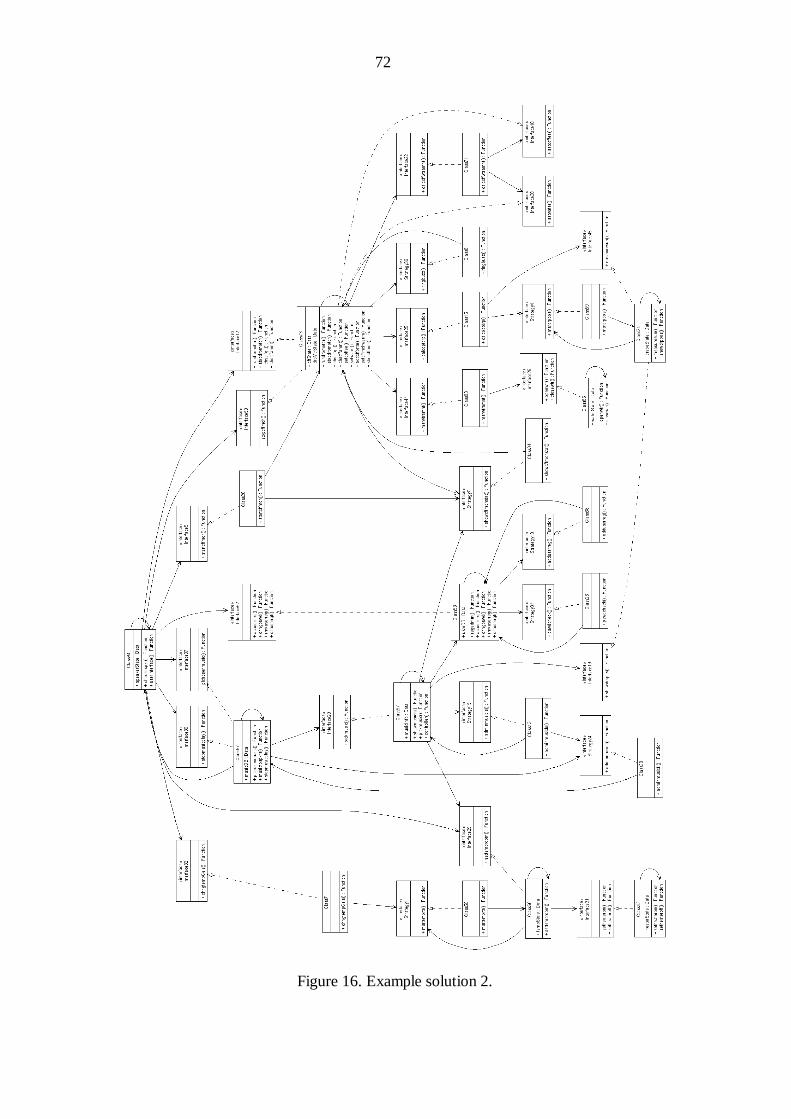
72
Figure 16. Example solution 2.

73
A solution that takes good advantage of the message dispatcher is depicted inFigure 17. Here the structure is not as clear as in Figures 15 and 16, and there are moredependencies between classes as in the solution in Figure 15. However, the solution ismore modifiable, as many calls happen through the dispatcher, and thus the classes arenot directly dependent on each other. For example, a good design decision in this casehas been to put the water control subsystem behind the dispatcher, thus alleviating thedependency between the coffee machine and the water control. The benefits andshortcomings of using a message dispatcher architecture style are not straightforward.The positive effect in modifiability and the negative effect in efficiency are easy to see,but how the dispatcher affects the structure, the “beauty”, of the solution, is morecomplicated. A wellplaced message dispatcher may actually simplify the structure, anddifferent components can easily be separated from the class diagram. A badlyplaceddispatcher, on the other hand, can make the solution extremely messy, if there are manyconnections to and from the dispatcher and the class division of the responsibilities is notextremely successful. The solution shown in Figure 17 is somewhere between theseextremes: the basic structure is successful enough so the use of message dispatcher doesnot make the solution completely incomprehensible, while some connections to thedispatcher clearly do more harm than good. In this case, the solution could benefit fromeither removing some connections to the dispatcher, or actually adding moreconnections, as the connections between classes would become more unified, and thedispatcher more central in the solution.
The Façade design pattern is not very often seen in the proposed solutions, asthere are few places where it can be implemented in the example system. Also, as it addscomplexity by bringing technical classes to the design, one might question the use ofboth a façade and a dispatcher in the same system. Figure 18 shows a solution where theFaçade pattern has been used efficiently. Here, the user interface and the main controllercall the façade interface instead of calling several responsibilities belonging to the manysubsystems that these special responsibilities control. However, in this case the structureis not very good – there are many small classes and responsibilities from nonrelatedsubsystems have been grouped in the same class, e.g., class 24 contains responsibilitiesfrom the water control subsystem and the music system. The message dispatcher has alsobeen brought to the system and used very inefficiently: only one responsibility uses thedispatcher to call two responsibilities through one interface.

74
Figure 17. Example solution 3.

75
Figure 18. Example solution 4.

76
7.3. Remarks on adjusting the parametersDuring the hundreds of test runs, some details about individual parameters and theirrelations to each other came apparent. I will now discuss the most remarkable findings ofthe tests.
Firstly, it could be seen that the fitness metrics have more influence to the finalsolution than the mutation probabilities. This came apparent when after nearly triplingthe probability of using a dispatcher, the amount of dispatchers or their users did notsignificantly increase. Affect of the modifiability quality metric could, however, be seeninstantly. Another point to make of mutation probabilities is that the probability of thecrossover operation had a bigger effect, and after first starting with a crossoverprobability of 10%, in the end it was lowered down to 4%, which gave noticeably betterresults. The biggest probabilities are for splitting and merging classes, as they deal withthe structure of the system. This has proven to be a good decision in optimizing theprobabilities, as structured solutions are indeed achieved: if the probabilities of the finetuning mechanisms would be overpowering, the solutions would most likely be morerandomly implementing the mechanisms, and the structure would rely heavily onrandomized class division given in the creation of the initial population. The probabilitiesof bringing a dispatcher to the system and introducing a Façade pattern are also quitehigh. Thus giving a large probability for bringing the dispatcher to the system gives thealgorithm a better chance to actually implement the mutations it chooses. The sameapplies for the façade mutation: implementing a façade requires quite a specific situationin the system, and thus often fails. Giving a larger probability will enhance the chances ofactually achieving a Façade pattern in the system.
Secondly, there is the balancing problem. Naturally, the best solution would beefficient, modifiable, and simple. Thus, all the different fitnesses should be valued.However, finding real weights with which solutions that have an overall quality is not atall straightforward. Although the different ranges of the subfitnesses have been takeninto account, some subfitnesses are still easier to affect, and thus achieve higher valueswith less work. For example, the positive modifiability and negative efficiency bothmeasure the amount of dispatcher connections, and the overall values of these subfitnesses have been balanced so that the values are in the same range. However, whenmeasuring the negative efficiency of a system, the number of dispatcher connections ismultiplied with the call cost of the needed responsibility. This means that a singledispatcher connection has more effect in the efficiency than in positive modifiability.Thus, the weight for positive modifiability must be substantially higher than the weightfor negative efficiency if one wants to achieve solutions that use the dispatchereffectively.

77
Balancing the weights is a difficult combinatorial optimization task also from theviewpoint of achieving solutions that would not have any big weaknesses. “Heavy”weights easily “cover” each other: a high positive value in some area may “cover” a highnegative value, and leave the final value higher than that of other solutions which mayhave more balanced values, thus resulting in a solution with both very desirable and veryundesirable qualities.
A particular balancing problem is in the structure, as the optimum solution wouldinclude mediumsized classes. However, the current metrics favor either very large(efficiency and complexity) classes or very small classes (modifiability). Large classesachieve high values from both positive efficiency and complexity, while small classesincluding only one or two responsibilities receive very small penalties from negativemodifiability, hence keeping the overall fitness value quite high even though the positivemetric value also stays small. This is actually a reverse situation of the “covering”discussed earlier: in this case both the positive and the negative values stay so small thatthe overall fitness value will still remain within the average and survive through manygenerations.
On a more detailed level, there are some restrictions regarding the fitness weightsthat should be considered. Firstly, the weights of complexity and positive efficiencyshould be quite similar, and quite low in relation to other metrics. Otherwise the numberof classes will be very small, and the modifiability fitness will not be able to develop. Atworst the solution only consists of a single class. Secondly, there is a delicate balancebetween negative efficiency and positive modifiability. The weight of positivemodifiability should be at least five times higher than that of negative efficiency if onewants many users for the message dispatcher. Finally, the weight for negativemodifiability should be kept within the same range as the weights for efficiency, but canbe slightly higher. These observations are in the case when all quality metrics are usedfor evaluation.
To conclude: there are no absolute rules as to how the weights can be assigned, asthey have a “seesaw” effect. By valuing some quality, another quality is hard to achieve.Rather, it should be attempted to balance the weights in such a way that no quality iscompletely overshadowed, thus making such a solution able that is somehow valued byall the quality aspects.

78
8. Conclusions
8.1. Presenting the resultsI have presented a novel approach to software architecture design in the field of searchbased software engineering. In this thesis I have taken a more abstract approach than theresearch done in the field so far as the structure of a software system is merely based onthe concept of responsibilities, and no information of actual operations is known.Another contribution is to experiment with building a completely new architecture andnot merely moving pieces in a readymade system as done previously (see Chapter 4).
The results presented in Chapter 7 show that it is possible to design softwarearchitectures with this approach. Sensible solutions are achieved, and they can becontrolled with the selection of fitness metrics – meaning that the construction of thearchitecture does indeed follow certain logic and is not completely random. Thesolutions mainly fell into two categories; either they had a good structure or theyefficiently used design patterns and the dispatcher architecture style. This is natural, aswhen weighting efficiency, the structure was kept quite simple, and while weightingmodifiability, design patterns and the dispatcher were vary much favored. Naturally,when neither quality aspect was weighted over the other, solutions were achieved thatcould be categorized as “somewhere in between”, i.e., solutions with a good structureand some usage of interfaces and maybe one connection to the dispatcher, or good usageof the finetuning mechanisms and some structure. However, a truly good solution is onewhere the quality can be seen instantly – an average solution does not provide any newinsights, as its biggest strength is actually its lack of weaknesses.
From the point of architecture design and architecture evaluation, theimplementation presented here provides a strong starting point for further developmentwhere the common “laws” concerning architectural design can be taken more intoaccount, thus ensuring quality solutions more consistently. In traditional architecturedesign, the software architect has the requirements for the system, and attempts to piecethe respective operations together so the solution reaches high values when “measured”by some quality attributes. In this approach, the genetic algorithm actually evaluates alarge number of architectures simultaneously, thus traversing through solutions a humanarchitect would not have the time or the imagination to think of. Hence, as these initialtests already show that the implementation is able to find solutions greatly valued evenafter human analysis, this approach could affectively cut down the time used inarchitecture design as well as provide innovative solutions either as a starting point forfurther design or as ready architectures.
From the point of searchbased software engineering and especially software designwith the help of metaheuristic search algorithms, this thesis clearly makes a contribution

79
to the field. As the starting point is raw data, and not a ready architecture, this approachgives the implementation a significantly freer traverse through the search space, thusresulting in more innovative solutions. When given a ready architecture, it can beassumed that the architecture is already of good quality. Thus, it might prove quitedifficult to find such modifications to the architecture that would actually improve thefitness value. The higher level of abstractness in architecture representation also providesa better starting point for constructing architectures, as the logical entities in softwaresystems do not always straightforwardly follow the structural or operational entities.
To conclude, the most important overall result of this thesis is that the approachtaken here appears reasonably successful. An architecture can be designed with the helpof a genetic algorithm with only abstract level knowledge of the architecture’s contentsand with no ready starting point.
8.2. Success evaluationAs discussed, the implementation was successful in proving that the selected approachwas a good one. The produced solutions were also successful in either providing a goodstructure or good usage of communication mechanisms in the architecture. I will nowdiscuss the main contributors to the success and also what could still be improved.
Firstly, the very basic elements needed for the algorithm to operate proved to be wellchosen. That is, the modeling, mutations and crossover discussed in Chapter 5, providedthe kind of basis for the algorithm to operate that it was possible to modify thearchitecture in such ways that would provide quality solutions.
Secondly, the fitness metrics proved to be very powerful, as weighting one fitnessvalue over another showed instantly in the produced solutions. It should be emphasizedthat enhancing the fitness values by taking into account interfaces and dispatchers wasnot based on anything found in the literature, but was constructed by logically evaluatingwhere these mechanisms would be best used. The grouping of different fitness metricsinto clear subfitnesses proved to be powerful, thus making it a contribution of its own.
Finally, there is obviously much that can still be improved. The ultimate goal wouldbe to consistently find solutions that are good from every quality aspect. Currentlysolutions with a high quality in any aspect are not consistent, and hardly any solutionsare found with a good overall quality. Another improvement area lies within the“legality” of the produced architecture. The major reasons for not receiving even betterresults at this stage lies in the optimization problem with different fitness metrics.Naturally, the mutation probabilities also have impact in the solution, but as theimplementation provided solutions from both “quality categories” by using the same setof probabilities, it is safe to assume that some sort of optimum combination of mutationprobabilities has actually been found. As a result, further development lies more withinthe set of fitness weights in terms of parameter optimization.

80
Overall, it can be stated that the work was successful. The main research questionwas whether the selected approach would even be possible and sufficient enough toproduce quality software architectures. As this was achieved, and there are clear views asto which direction the research could be taken, the implementation can indeed be viewedas successful, and the approach deemed possible.
8.3. Future workThe work presented in this thesis has been a followup to the work done in my Master’sthesis, as the basic implementation has been taken further by introducing “architecturelaws”, design patterns, a more refined fitness function, and parameterizing mutationprobabilities and other variables regarding the genetic algorithm. As the results havesignificantly improved from those introduced previously, there are even more grounds tofurther continue the work. There are still many ways with which the currentimplementation can be further developed and improved.
Firstly, the finetuning mechanisms can be put to better use by introducing morearchitecture styles and design patterns to the model. Naturally, the more mutations areintroduced, the more the solution space grows. However, when the algorithm is notrestricted to only a minimal amount of options in developing the architecture, thechances of finding a solution that is very close to the optimal increase significantly.
Secondly, more metrics should be considered, as evaluating an architecture frommerely three quality viewpoints is hardly the case in a real world situation. Asincorporating more “architecture laws” would also take care of some basic structuraldecisions, the existing metrics could also be adjusted to more effectively evaluate thestructural decisions that are actually made by mutations and crossover.
Thirdly, the evaluation can be improved by making the fitness function dynamic. Itcould only evaluate the structure in the first generations, and then begin to evaluate theusage of finetuning mechanisms when they sufficiently exist in the architecture. As thesemechanisms are not present in the initial population, this kind of adjusted fitness functioncould provide more quality structures.
Fourthly, another metaheuristic search algorithm could be implemented in order tomake a comparison between its results and the results provided by the genetic algorithm.If it is possible to model an architecture and achieve good results from, e.g., animplementation with simulated annealing, it could be researched whether the strengths ofboth the new and initial algorithm implementations could be combined.
Finally, the quality of the implementation can be improved by producing informationof the solution in a format that can be easily modified, such as XMI.
To conclude: the work and results presented in this thesis are the beginning in aresearch approach with many possibilities. The basis has been made by producing amodel and initial operations which can be further developed and combined to achievesignificant results in the field of searchbased software engineering.

81
References[Alba and Chicano, 2007] E. Alba and J.F. Chicano, Software project management with
GAs, Information Sciences 177, 2007, 23802401.[Amoui et al., 2006] M. Amoui, S. Mirarab, S. Ansari and C. Lucas, A genetic algorithm
approach to design evolution using design pattern transformation, InternationalJournal of Information Technology and Intelligent Computing 1 (1, 2), June/August, 2006, 235245.
[Bass et al., 1998] L. Bass, P. Clements and R. Kazman, Software Architecture inPractice, AddisonWesley, 1998.
[Blickle, 1996] T. Blickle, Evolving compact solutions in genetic programming: a casestudy In: H. Voigt, W. Ebeling, I. Rechenberg, and H. Schwefel (eds.), ParallelProblem Solving from Nature IV, Proceedings of the International Conferenceon Evolutionary Computation, LNCS 1141, 1996, 564573.
[Burgess, 1995] C.J. Burgess, A genetic algorithm for the optimisation of amultiprocessor computer architecture, In: GALESIA'95, 1st IEE/IEEEInternational Conference on Genetic Algorithms in Engineering Systems:Innovations and Applications, IEE Conference Publication 414, Sept. 1995, 3944
[Canfora et al., 2005] G. Canfora, M. Di Penta, R. Esposito, M. L. Villani, An approachfor qoSaware service composition based on genetic algorithms, In: GECCO2005: Proceedings of the Genetic and Evolutionary Computation Conference,June 2005, 1069–1075.
[Che et al., 2003] Y. Che, Z. Wang and X. Li, Optimization parameter selection bymeans of limited execution and genetic algorithms, In: X. Zhou et al. (Eds.):APPT 2003, LNCS 2834, 2003, 226–235.
[Chidamber and Kemerer, 1994] S.R. Chidamber and C.F. Kemerer, A metrics suite forobject oriented design. IEEE Transactions on Software Engineering 20 (6),1994, 476492.
[Clarke et al., 2003] J. Clarke, J. J. Dolado, M. Harman, R. M. Hierons, B. Jones, M.Lumkin, B. Mitchell, S. Mancoridis, K. Rees, M. Roper and M. Shepperd,Reformulating Software Engineering as a Search Problem, IEE Proceedings Software, 150 (3), 2003, 161175.
[Di Penta et al., 2005] M. Di Penta, M. Neteler, G. Antoniol and E. Merlo, A languageindependent software renovation framework, The Journal of Systems andSoftware 77, 2005, 225240.
[Dick and Jha, 1998] R.P. Dick and N.K. Jha, MOGAC: A multiobjective geneticalgorithm for the cosynthesis of hardwaresoftware embedded systems. IEEETrans. on ComputerAided Design of Integrated Circuits and Systems 17 (10),

82
Oct. 1998, 920935.[Doval et al., 1999] D. Doval, S. Mancoridis and B.S. Mitchell, Automatic clustering of
software systems using a genetic algorithm, In: Proceedings of the SoftwareTechnology and Engineering Practice, 1999, 7382.
[Du Bois and Mens, 2003] B. Du Bois and T. Mens, Describing the impact ofrefactoring on internal program quality. In: Proceedings of the InternationalWorkshop on Evolution of LargeScale Industrial Software Applications 2003,3748.
[GraphViz, 2007] http://www.graphviz.org, checked 17.1.2008.[Gamma et al., 1995] E. Gamma, R. Helm, R. Johnson and J. Vlissides, Design Patterns,
Elements of Reusable ObjectOriented Software. AddisonWesley, 1995.[Grunske, 2006] L. Grunske, Identifying "good" architectural design alternatives with
multiobjective optimization strategies. In: Proceeding of the 28th InternationalConference on Software Engineering, Shanghai, China, 2006, 849 852.
[Harman et al., 2002] M. Harman, R. Hierons and M. Proctor, A new representation andcrossover operator for searchbased optimization of software modularization. In:GECCO 2002: Proceedings of the Genetic and Evolutionary ComputationConference, July 2002, 1351–1358.
[Harman and Tratt, 2007] M. Harman and L. Tratt, Pareto optimal search basedrefactoring at the design level, In: GECCO 2007: Proceedings of the Geneticand Evolutionary Computation Conference, 2007, 11061113.
[IEEE, 2000] IEEE Recommended Practice for Architectural Description of SoftwareIntensive Systems. IEEE Standard 14712000, 2000.
[Jaeger and Mühl, 2007] M.C. Jaeger and G. Mühl, QoSbased selection of services: theimplementation of a genetic algorithm, In T. Braun, G. Carle and B. Stiller(Eds.): Kommunikation in Verteilten Systemen (KiVS) 2007 Workshop: ServiceOriented Architectures und ServiceOriented Computing, VDE Verlag, March2007, 359371.
[Kazman et al., 2000] R. Kazman, M. Klein and P. Clements, ATAM: Method forarchitecture evaluation, CarnegieMellon University, Technical report CMU/SEI2000TR004, August 2000.
[Koskimies ja Mikkonen, 2005] K. Koskimies ja T. Mikkonen, Ohjelmistoarkkitehtuurit.Talentum, 2005.
[Le Hanh et al., 2001] V. Le Hanh, K. Akif, Y. Le Traon and JM. Jézéquel, Selectingan efficient OO integration testing strategy: an experimental comparison of actualstrategies. In: J. Lindskov Knudsen (Ed.): ECOOP 2001, LNCS 2072, 2001,381401.
[Losavio et al., 2004] F. Losavio, L. Chirinos, A. Matteo, N. Lévy and A. RamdaneCherif, ISO quality standards for measuring architectures. The Journal of

83
Systems and Software 72, 2004, 209223.[Mens and Demeyer, 2001] T. Mens and S. Demeyer, Future trends in evolution metrics,
In: Proc. Int. Workshop on Principles of Software Evolution, 2001, 8386.[Michalewicz, 1992] Z. Michalewicz, Genetic Algorithms + Data Structures =
Evolutionary Programs. SpringerVerlag, 1992.[de Miguel et al.,2000 ] M. de Miguel, T. Lambolais, S. Piekarec, S. BetgéBrezetz and
J, Péquery, Automatic generation of simulation models for the evaluation ofperformance and reliability of architectures specified in UML, In: Revised Papersfrom the Second International Workshop on Engineering Distributed Objects,LNCS 1999, 2000, 83–101.
[Mitchell, 1996] M. Mitchell, An Introduction to Genetic Algorithms. MIT Press, 1996.[O’Keeffe and Ó Cinnéide, 2004] M. O’Keeffe and M. Ó Cinnéide, Towards automated
design improvements through combinatorial optimization, In: Workshop onDirections in Software Engineering Environments (WoDiSEE2004), W2SWorkshop 26th International Conference on Software Engineeering, 2004, 7582.
[O’Keeffe and Ó Cinnéide, 2007] M. O’Keeffe and M. Ó Cinnéide, Getting the mostfrom searchbased refactoring In: GECCO 2007: Proceedings of the Genetic andEvolutionary Computation Conference, 2007, 11141120.
[Räihä, 2008] O. Räihä, Applying Genetic Algorithms in Software Architecture Design,University of Tampere, Department of Computer Sciences, M.Sc. Thesis,February 2008.
[Reeves, 1995] C. R. Reeves, Modern Heuristic Techniques for CombinatorialProblems. McGrawHill Book Company, 1995.
[Rela, 2004] L. Rela, Evolutionary computing in searchbased software engineering,Lappeenranta University of Technology, Department of Information Technology,M.Sc. Thesis, 2004.
[Rosenberg and Hyatt, 1997] L. Rosenberg and L. Hyatt, Software quality metrics forobjectoriented design, available ashttp://satc.gsfc.nasa.gov/support/CROSS_APR97/oocross.PDF, checked12.9.2007.
[Sahraoui et al., 2000] H.A. Sahraoui, R. Godin and T. Miceli, Can metrics help bridgingthe gap between the improvement of OO design quality and its automation? In:Proc. of the International Conference on Software Maintenance (ICSM ’00),154162, available ashttp://www.iro.umontreal.ca/~sahraouh/papers/ICSM00.pdf, checked 12.9.2007.
[Salomon, 1998] R. Salomon, Short notes on the schema theorem and the building blockhypothesis in genetic algorithms, In: Evolutionary Programming VII, LNCS1447, 1998, 113122.

84
[Seng et al., 2005] O. Seng, M. Bauyer, M. Biehl and G. Pache, Searchbasedimprovement of subsystem decomposition, In: GECCO 2005: Proceedings of theGenetic and Evolutionary Computation Conference, 2005, 1045 – 1051.
[Seng et al., 2006] O. Seng, J. Stammel and D. Burkhart, Searchbased determination ofrefactorings for improving the class structure of objectoriented systems, In:GECCO 2006: Proceedings of the Genetic and Evolutionary ComputationConference, 2006, 1909–1916.
[UMLGraph, 2007] http://www.umlgraph.org, checked 17.1.2008.

Appendix ACase study data
The electronic home control system case study data. If the Depending responsibilitiescolumn has the value 0, then no responsibility uses the corresponding responsibility i.Type “f” stands for “functional” and “d” for “data”. Groups of functional responsibilitiesforming a subsystem are separated by a bolded line.
Responsibilitynumber
Dependingresponsibilities
Executiontime(ms)
Parametersize
Frequency
Variability
Callcost
Name Type
1 2,5 30 5.0 2 1 30 pswdcheck f2 3,4,6,7, 47 40 6.0 1 1 40 regadmin f3 48 30 6.0 1 1 30 actuserreg f4 3 30 6.0 1 1 30 adduserreg f5 48 50 8.0 1 1 50 chngpswd f6 48 60 2.0 1 1 60 rmvuserreg f7 48 70 5.0 1 1 70 setuserrgt f
8 47,48 40 8.0 3 1 40 settemproom f9 8,10 60 4.0 3 2 60 msrtemprtr f10 48 20 4.0 3 1 20 chngtempCels f11 8 50 1.0 2 2 50 setheateron f12 8 50 1.0 1 2 50 setheateroff f
13 14,47 70 9.0 5 2 70 adminmusicls f14 15 90 9.0 5 3 90 showmusicls f15 17 70 6.5 5 1 70 pickmusic f16 13,17,20 110 10.0 5 1 110 adminmusicfl f17 48 100 8.5 5 1 100 plchosenmusic f18 17 60 3.0 1 2 60 choosespkr f19 17 60 3.5 5 1 60 musictospkrs f20 48 50 3.0 1 1 50 stopmusicplay f
21 24 80 7.0 3 1 80 measuresun f22 23,24 80 7.0 3 1 80 msrdrppos f23 47 70 5.0 3 1 70 showdrppos f24 25,26 90 6.5 3 3 90 calcoptdrp f

25 48 60 2.0 2 1 60 rundrpmotor f26 48 50 1.0 2 1 50 stopdrpmotor f
27 31,32,37,47
110 10.5 2 2 110 showcffmchstat f
28 48 40 5.0 2 3 40 chscffqlt f29 48 40 5.0 2 3 40 chscffamnt f30 28,29 50 6.0 2 1 50 calccffwtramnt f31 30 50 3.5 2 1 50 setcoffee f32 30 50 3.5 2 1 50 setwater f33 32 50 2.5 2 1 50 msrwtramnt f34 31 30 2.0 2 1 30 addcffprtn f35 33 30 1.0 2 2 30 openwtr f36 33 30 1.0 2 2 30 closewtr f37 48 70 2.0 2 2 70 startcffmch f38 37 70 3.5 2 1 70 setcffmchwarm f39 48 50 2.0 2 1 50 stopcffmch f40 39 20 2.0 2 1 20 ringbuzz f
41 1,2,3,4,5,6,7
10 2.0 7 1 10 userDB d
42 16,17,19 10 2.0 3 1 10 musicDB d43 13,14,15 10 2.0 3 1 10 musicInfo d44 21,22,23 10 2.0 3 1 10 drapeState d45 27,28,29,
31, 32, 34,38, 39, 40
10 2.0 5 1 10 cffState d
46 8,9 10 2.0 3 1 10 tempState d47 0 10 2.0 3 2 10 controller f48 0 10 2.0 14 2 10 userInterface f49 11,12 10 2.0 2 1 10 heaterState d50 35,36 10 2.0 2 1 10 waterState d51 18 10 2.0 1 1 10 speakerState d52 25,26 10 2.0 2 1 10 drpMtrState d
Table 1. Case study responsibility set.

Appendix BFitness study parameters
Table 3. Fitness weights.
Table 4. Fitness weights when modifiability overweighted.
Table 2. Mutation parameters
Table 5. Fitness weightswhen efficiency overweighted.
Mutation ProbabilitySplit class 0.08Merge classes 0.06Connect dispatcher 0.1Remove dispatcher 0.04Introduce interface 0.02Remove interface 0.03Introduce newdispatcher 0.09Remove emptydispatcher 0.03Introduce Façade 0.15Remove Façade 0.02Introduce Strategy 0.1Remove Strategy 0.02Use variability 0.08Remove variability 0.06Null 0.08Crossover 0.04
Subfitness WeightPositive modifiability 10Negative modifiability 10Positive efficiency 10Negative efficiency 10Complexity 10
Subfitness WeightPositive modifiability 100Negative modifiability 50Positive efficiency 5Negative efficiency 5Complexity 5
Subfitness WeightPositive modifiability 5Negative modifiability 5Positive efficiency 100Negative efficiency 50Complexity 5

Appendix CExample solutions’ parameters
Example solution 1
Table 8. Fitness weightsfor example solution 1.
Table 7. Mutation probabilities for example solution 1.
Mutation ProbabilitySplit class 0.09Merge classes 0.06Connect dispatcher 0.13Remove dispatcher 0.03Introduce interface 0.02Remove interface 0.03Introduce newdispatcher 0.1Remove emptydispatcher 0.03Introduce Façade 0.13Remove Façade 0.02Introduce Strategy 0.08Remove Strategy 0.02Use variability 0.08Remove variability 0.06Null 0.08Crossover 0.04
Subfitness WeightPositive modifiability 45Negative modifiability 15Positive efficiency 10Negative efficiency 5Complexity 8

Example solution 2
Table 10. Fitness weightsfor example solution 2.
Table 9. Mutation probabilities for example solution 2.
Mutation ProbabilitySplit class 0.08Merge classes 0.06Connect dispatcher 0.1Remove dispatcher 0.04Introduce interface 0.02Remove interface 0.03Introduce newdispatcher 0.09Remove emptydispatcher 0.03Introduce Façade 0.15Remove Façade 0.02Introduce Strategy 0.1Remove Strategy 0.02Use variability 0.08Remove variability 0.06Null 0.08Crossover 0.04
Subfitness WeightPositive modifiability 20Negative modifiability 15Positive efficiency 5Negative efficiency 5Complexity 10

Example solution 3
Table 12. Fitness weightsfor example solution 3.
Table 11. Mutation probabilities for example solution 3.
Mutation ProbabilitySplit class 0.08Merge classes 0.06Connect dispatcher 0.1Remove dispatcher 0.04Introduce interface 0.02Remove interface 0.03Introduce newdispatcher 0.09Remove emptydispatcher 0.03Introduce Façade 0.15Remove Façade 0.02Introduce Strategy 0.1Remove Strategy 0.02Use variability 0.08Remove variability 0.06Null 0.08Crossover 0.04
Subfitness WeightPositive modifiability 45Negative modifiability 15Positive efficiency 15Negative efficiency 2Complexity 8

Example solution 4
Table 14. Fitness weightsfor example solution 4.
Table 13. Mutation probabilities for example solution 4.
Mutation ProbabilitySplit class 0.08Merge classes 0.06Connect dispatcher 0.1Remove dispatcher 0.04Introduce interface 0.02Remove interface 0.03Introduce newdispatcher 0.09Remove emptydispatcher 0.03Introduce Façade 0.15Remove Façade 0.02Introduce Strategy 0.1Remove Strategy 0.02Use variability 0.08Remove variability 0.06Null 0.08Crossover 0.04
Subfitness WeightPositive modifiability 45Negative modifiability 15Positive efficiency 10Negative efficiency 5Complexity 8