evolutionary and computational advantages of ... · evolutionary and computational advantages of...
TRANSCRIPT

Evolutionary and ComputationalAdvantages of
Neuromodulated Plasticity
Andrea Soltoggio
A thesis submittedto The University of Birmingham
for the degree of Doctor of Philosophy
School of Computer ScienceThe University of BirminghamBirmingham B15 2TTUnited Kingdom
October 2008

ii

Abstract
The integration of modulatory neurons into evolutionary artificial neu-
ral networks is proposed here. A model of modulatory neurons was devised
to describe a plasticity mechanism at the low level of synapses and neu-
rons. No initial assumptions were made on the network structures or on the
system level dynamics. The work of this thesis studied the outset of high
level system dynamics that emerged employing the low level mechanism
of neuromodulated plasticity. Fully-fledged control networks were designed
by simulated evolution: an evolutionary algorithm could evolve networks
with arbitrary size and topology using standard and modulatory neurons
as building blocks.
A set of dynamic, reward-based environments was implemented with
the purpose of eliciting the outset of learning and memory in networks.
The evolutionary time and the performance of solutions were compared for
networks that could or could not use modulatory neurons. The experimen-
tal results demonstrated that modulatory neurons provide an evolutionary
advantage that increases with the complexity of the control problem. Net-
works with modulatory neurons were also observed to evolve alternative
neural control structures with respect to networks without neuromodula-
tion. Different network topologies were observed to lead to a computational
advantage such as faster input-output signal processing.
The evolutionary and computational advantages induced by modulatory
neurons strongly suggest the important role of neuromodulated plasticity for
the evolution of networks that require temporal neural dynamics, adaptivity
and memory functions.

ii

Acknowledgements
Thanks firstly to John Bullinaria who, rather than teaching me, offered me
with great patience and understanding the chance to learn. His generous
support and example have been essential for my growth and greatly fulfilling
during all my Ph.D. What I have learnt from him goes well beyond the work
of these pages.
Thanks to Dario Floreano for our fruitful and enlightening collaboration
from which I have taken an extraordinary valuable guidance. Thanks to Jon
Rowe, Alastair Channon, Peter Coxhead, Peter Durr and Claudio Mattiussi
for their availability and constructive discussions.
The work in this thesis was influenced by a great number of people who,
either by personal contact or through writing, enriched my knowledge and
stimulated my imagination with continuous suggestions and ideas. Any
attempt to list their names here would be inadequate and incomplete, but
I am most grateful to all of them.
I would like to acknowledge the very important contributions of those
who appreciated my work showing their interest and commenting the draft
of this thesis. Many thanks go to Diego Federici, Ben Jones, Edward Robin-
son, and Natalja Prokoptsova.
Finally, by reaching the end of this four-year project that took a fair
amount of time and effort, my attention is drawn to the people that have
been important to me in these years and before. I dedicate these last lines to
all whom have given me everything that is difficult to describe scientifically.
iii

Contents
1 Introduction 1
1.1 Note to Chapter 1 . . . . . . . . . . . . . . . . . . . . . . . 1
1.2 Neural Systems . . . . . . . . . . . . . . . . . . . . . . . . . 1
1.3 Artificial Neural Controllers . . . . . . . . . . . . . . . . . . 2
1.4 About the Thesis . . . . . . . . . . . . . . . . . . . . . . . . 4
1.4.1 Research Questions . . . . . . . . . . . . . . . . . . . 6
1.4.2 Hypotheses and Method . . . . . . . . . . . . . . . . 7
1.4.3 Contribution to Knowledge . . . . . . . . . . . . . . 8
1.4.4 Structure of the Thesis . . . . . . . . . . . . . . . . . 9
1.4.5 Publications Resulting From This Study . . . . . . . 10
2 Neural Networks 12
2.1 Biological Networks . . . . . . . . . . . . . . . . . . . . . . . 13
2.1.1 The Molecular and Cellular Level . . . . . . . . . . . 14
2.1.2 The Diffuse Modulatory Systems:
Modulation at the System Level . . . . . . . . . . . . 18
2.1.3 Neuromodulated or Heterosynaptic Plasticity:
Modulation at the Cellular Level . . . . . . . . . . . 21
2.2 Neural Models . . . . . . . . . . . . . . . . . . . . . . . . . . 27
2.2.1 Neuron Models . . . . . . . . . . . . . . . . . . . . . 28
2.2.2 Neural Architectures . . . . . . . . . . . . . . . . . . 32
2.2.3 Learning and Plasticity . . . . . . . . . . . . . . . . . 35
iv

CONTENTS
3 Phylogenetic Search 48
3.1 Motivations . . . . . . . . . . . . . . . . . . . . . . . . . . . 48
3.2 Overview of Algorithms for
Artificial Evolution . . . . . . . . . . . . . . . . . . . . . . . 50
3.2.1 Set up of an Evolutionary Algorithm . . . . . . . . . 51
3.2.2 Fitness Design . . . . . . . . . . . . . . . . . . . . . . 52
3.3 Design and Evolution of ANNs . . . . . . . . . . . . . . . . 56
3.3.1 Development, Evolution and Adaptation . . . . . . . 57
4 Dynamic, Reward-based Scenarios 66
4.1 Control Problems for Online Learning . . . . . . . . . . . . . 66
4.1.1 Why dynamic scenarios . . . . . . . . . . . . . . . . . 67
4.1.2 Why reward-based scenarios . . . . . . . . . . . . . . 67
4.1.3 Types of uncertainties . . . . . . . . . . . . . . . . . 68
4.1.4 Hidden and non-hidden rewards . . . . . . . . . . . . 69
4.2 n-armed Bandit Problems . . . . . . . . . . . . . . . . . . . 72
4.3 The Bee Foraging Problem . . . . . . . . . . . . . . . . . . . 73
4.3.1 The Simulated Bee . . . . . . . . . . . . . . . . . . . 75
4.3.2 Scenarios . . . . . . . . . . . . . . . . . . . . . . . . 76
4.3.3 Correspondence Between Fitness and Behaviour . . . 78
4.4 T-mazes . . . . . . . . . . . . . . . . . . . . . . . . . . . . . 79
4.4.1 Inputs and Outputs . . . . . . . . . . . . . . . . . . . 81
4.4.2 Correspondence Between Fitness and Behaviour . . . 83
4.5 Temporal Dynamics . . . . . . . . . . . . . . . . . . . . . . . 86
5 Model and Design for Neuromodulation 87
5.1 A Model for Modulatory Neurons . . . . . . . . . . . . . . . 87
5.1.1 Target of Modulation . . . . . . . . . . . . . . . . . . 91
5.1.2 Default Plasticity . . . . . . . . . . . . . . . . . . . . 91
5.2 A General Plasticity Rule . . . . . . . . . . . . . . . . . . . 92
5.2.1 Types of Plasticity . . . . . . . . . . . . . . . . . . . 93
5.3 The Search Algorithm . . . . . . . . . . . . . . . . . . . . . 98
v

CONTENTS
5.3.1 Genotypical Representation . . . . . . . . . . . . . . 99
5.3.2 Evolution and Genetic Operators . . . . . . . . . . . 99
5.3.3 Phenotypical Expression . . . . . . . . . . . . . . . . 103
5.3.4 Alternative Algorithms . . . . . . . . . . . . . . . . . 105
5.4 Hypotheses . . . . . . . . . . . . . . . . . . . . . . . . . . . 107
5.4.1 Evolutionary Advantages . . . . . . . . . . . . . . . . 107
5.4.2 Computational Advantages . . . . . . . . . . . . . . . 108
6 Empirical Results 110
6.1 Structure of the Experiments . . . . . . . . . . . . . . . . . 110
6.2 Solving n-armed Bandit Problems: A Minimal Model . . . . 112
6.2.1 Summary . . . . . . . . . . . . . . . . . . . . . . . . 112
6.2.2 Plasticity Rule and Design Method . . . . . . . . . . 114
6.2.3 Inputs-Output Sequences . . . . . . . . . . . . . . . . 114
6.2.4 Design and Choice of the Model . . . . . . . . . . . . 115
6.2.5 Analysis of the Model . . . . . . . . . . . . . . . . . 116
6.2.6 Conclusion . . . . . . . . . . . . . . . . . . . . . . . . 125
6.3 Solving Control Problems without Neuromodulation: Exper-
iments with an Agent in a T-maze and Foraging Bee . . . . 127
6.3.1 Summary . . . . . . . . . . . . . . . . . . . . . . . . 127
6.3.2 Plasticity Rules . . . . . . . . . . . . . . . . . . . . . 127
6.3.3 Experimental Settings . . . . . . . . . . . . . . . . . 128
6.3.4 Results . . . . . . . . . . . . . . . . . . . . . . . . . . 129
6.3.5 Conclusion . . . . . . . . . . . . . . . . . . . . . . . . 134
6.4 Introducing Evolving Modulatory Topologies to Solve the
Foraging Bee Problem . . . . . . . . . . . . . . . . . . . . . 135
6.4.1 Summary . . . . . . . . . . . . . . . . . . . . . . . . 135
6.4.2 Implementation . . . . . . . . . . . . . . . . . . . . . 135
6.4.3 Genetic Algorithm . . . . . . . . . . . . . . . . . . . 138
6.4.4 Performance . . . . . . . . . . . . . . . . . . . . . . . 139
6.4.5 Levels of Adaptivity . . . . . . . . . . . . . . . . . . 140
vi

CONTENTS
6.4.6 Analysis of Networks . . . . . . . . . . . . . . . . . . 140
6.4.7 Conclusion . . . . . . . . . . . . . . . . . . . . . . . . 142
6.5 Advantages of Neuromodulation: Experiments in the T-maze
Problems . . . . . . . . . . . . . . . . . . . . . . . . . . . . . 149
6.5.1 Evolutionary Search . . . . . . . . . . . . . . . . . . 149
6.5.2 Experimental Results . . . . . . . . . . . . . . . . . . 149
6.5.3 Analysis and Discussion . . . . . . . . . . . . . . . . 153
6.5.4 Functional Role of Neuromodulation . . . . . . . . . 156
6.5.5 Conclusion . . . . . . . . . . . . . . . . . . . . . . . . 161
6.6 Increasing the Decision Speed in a Control Problem with
Neuromodulation . . . . . . . . . . . . . . . . . . . . . . . . 162
6.6.1 Summary . . . . . . . . . . . . . . . . . . . . . . . . 162
6.6.2 Network Topologies . . . . . . . . . . . . . . . . . . . 162
6.6.3 Decision Speed . . . . . . . . . . . . . . . . . . . . . 163
6.6.4 Enforcing Speed . . . . . . . . . . . . . . . . . . . . . 167
6.6.5 Conclusion . . . . . . . . . . . . . . . . . . . . . . . . 170
6.7 A Reduced Plasticity Model: Evolving Learning with Pure
Heterosynaptic Plasticity . . . . . . . . . . . . . . . . . . . . 172
6.7.1 Summary . . . . . . . . . . . . . . . . . . . . . . . . 172
6.7.2 Results . . . . . . . . . . . . . . . . . . . . . . . . . . 173
6.7.3 Conclusion . . . . . . . . . . . . . . . . . . . . . . . . 174
6.8 Adaptation without Rewards: An Evolutionary Advantage
of Neuromodulation . . . . . . . . . . . . . . . . . . . . . . . 175
6.8.1 Summary . . . . . . . . . . . . . . . . . . . . . . . . 175
6.8.2 Results . . . . . . . . . . . . . . . . . . . . . . . . . . 176
6.8.3 Conclusion . . . . . . . . . . . . . . . . . . . . . . . . 176
7 Conclusion 179
7.1 Summary of Main Findings . . . . . . . . . . . . . . . . . . 179
7.1.1 Contribution to Knowledge . . . . . . . . . . . . . . 181
7.2 Future Work . . . . . . . . . . . . . . . . . . . . . . . . . . . 184
vii

CONTENTS
7.2.1 Modulation of Neuron Output
and Multi-neuron Type Networks . . . . . . . . . . . 185
7.2.2 Neuromodulation with Continuous Time or Spiking
Models . . . . . . . . . . . . . . . . . . . . . . . . . . 186
7.2.3 Neuromodulation for Robotic Applications . . . . . . 187
7.2.4 Neural Dynamics and Structures for Learning . . . . 187
Glossary 195
References 195
viii

List of Figures
2.1 Golgi-stained neurons. Image from (Wikipedia, 2008). . . . . 14
2.2 Simplified drawing of a neuron cell . . . . . . . . . . . . . . 15
2.3 Simplified drawing of a synapse . . . . . . . . . . . . . . . . 16
2.4 Noradrenergic and dopaminergic diffuse systems . . . . . . . 20
2.5 Schemes of homo- and heterosynaptic mechanisms . . . . . . 23
2.6 Homo- and heterosynaptic plasticity . . . . . . . . . . . . . . 26
2.7 Basic model of a neural network . . . . . . . . . . . . . . . . 28
2.8 Functions for neuron output . . . . . . . . . . . . . . . . . . 29
2.9 Network architectures . . . . . . . . . . . . . . . . . . . . . . 33
3.1 Scheme of an evolutionary algorithm . . . . . . . . . . . . . 51
3.2 POE space . . . . . . . . . . . . . . . . . . . . . . . . . . . . 58
3.3 AGE genome . . . . . . . . . . . . . . . . . . . . . . . . . . 61
3.4 AGE devices . . . . . . . . . . . . . . . . . . . . . . . . . . . 61
4.1 Examples of reward policies . . . . . . . . . . . . . . . . . . 70
4.2 Illustration of a 3-armed bandit problem . . . . . . . . . . . 73
4.3 Simulated bee and flower field . . . . . . . . . . . . . . . . . 75
4.4 Inputs-output for the foraging bee . . . . . . . . . . . . . . . 77
4.5 Single T-maze with homing . . . . . . . . . . . . . . . . . . 80
4.6 Double T-maze with homing . . . . . . . . . . . . . . . . . . 81
4.7 Inputs-output in T-mazes . . . . . . . . . . . . . . . . . . . 82
5.1 Scheme illustrating the model of neuromodulation . . . . . . 88
5.2 Hyperbolic tangent for modulation . . . . . . . . . . . . . . 90
ix

LIST OF FIGURES
5.3 Graphical representation of the plasticity rules . . . . . . . . 95
5.3 Caption of Figure 5.3 . . . . . . . . . . . . . . . . . . . . . . 96
5.4 Spatial tournament selection . . . . . . . . . . . . . . . . . . 100
5.5 Fitness progress using a spatial tournament selection . . . . 101
5.6 Probability density functions for mutation . . . . . . . . . . 103
5.7 Distribution of initial weights . . . . . . . . . . . . . . . . . 104
5.8 Genotype-phenotype mapping . . . . . . . . . . . . . . . . . 106
5.8 Caption of Figure 5.8 . . . . . . . . . . . . . . . . . . . . . . 107
6.1 Structure of the controller and IO sequences . . . . . . . . . 113
6.2 One-neuron learning model . . . . . . . . . . . . . . . . . . . 117
6.3 Operant conditioning with 10 arms . . . . . . . . . . . . . . 118
6.4 Noise and learning rates . . . . . . . . . . . . . . . . . . . . 120
6.5 Trade-off with different learning rates . . . . . . . . . . . . . 121
6.6 Plastic connection weights . . . . . . . . . . . . . . . . . . . 122
6.7 Restoring a correct behaviour after a weight randomisation . 124
6.8 Fitness in the single T-maze . . . . . . . . . . . . . . . . . . 130
6.9 Fitness for the foraging bee . . . . . . . . . . . . . . . . . . 131
6.10 Example of a plastic network for the T-maze . . . . . . . . . 133
6.11 Example of a plastic network for the bee . . . . . . . . . . . 134
6.12 Example of AGE genome . . . . . . . . . . . . . . . . . . . . 136
6.13 Best and average fitness for the bee . . . . . . . . . . . . . . 139
6.14 Behaviour of a bee . . . . . . . . . . . . . . . . . . . . . . . 143
6.14 Caption of Figure 6.14 . . . . . . . . . . . . . . . . . . . . . 144
6.15 Example of the network of a well performing bee . . . . . . . 145
6.16 Test of a bee on scenario 4 . . . . . . . . . . . . . . . . . . . 146
6.17 Analysis of neural activity and weights . . . . . . . . . . . . 147
6.17 Caption of Figure 6.17 . . . . . . . . . . . . . . . . . . . . . 148
6.18 Box plots for the single T-maze . . . . . . . . . . . . . . . . 152
6.19 Box plots for the double T-maze . . . . . . . . . . . . . . . . 153
6.20 Example of a modulatory network . . . . . . . . . . . . . . . 154
6.21 Behaviour of an agent in the double T-maze . . . . . . . . . 155
x

LIST OF FIGURES
6.21 Caption of Figure 6.21 . . . . . . . . . . . . . . . . . . . . . 156
6.22 Fitness for standard and modulatory networks . . . . . . . . 157
6.23 Differential measurements of fitness . . . . . . . . . . . . . . 158
6.24 Example of a plastic network . . . . . . . . . . . . . . . . . 164
6.25 Values of the output signal . . . . . . . . . . . . . . . . . . . 165
6.26 Example of a modulatory network . . . . . . . . . . . . . . . 166
6.27 Fitness progress during evolution . . . . . . . . . . . . . . . 168
6.28 Box plots of performance with constrained timing . . . . . . 169
6.29 Performance using pure heterosynaptic plasticity . . . . . . . 173
6.30 Fitness progress during evolution with modulatory neurons . 177
6.31 Fitness progress during evolution without modulatory neurons177
7.1 Photos of small wheeled robots . . . . . . . . . . . . . . . . 188
7.2 Neural activity in the double T-maze . . . . . . . . . . . . . 189
7.3 Neural activity in the double T-maze with homing . . . . . . 190
xi

List of Tables
2.1 Examples of neurotransmitter chemicals. . . . . . . . . . . . 19
4.1 Reward policies for the foraging bee . . . . . . . . . . . . . . 78
6.1 Performance of the one-neuron model on 3-, 10-, and 20-
armed bandit problems. . . . . . . . . . . . . . . . . . . . . 118
6.2 Number of neurons and connections in plastic networks . . . 133
6.3 Parameters for the evolutionary search . . . . . . . . . . . . 150
6.4 Parameters for the environments . . . . . . . . . . . . . . . . 150
6.5 Parameters for the neural networks . . . . . . . . . . . . . . 151
xii

Chapter 1
Introduction
1.1 Note to Chapter 1
This chapter has the purpose of introducing the topic, scope and findings
of this thesis in a few concise pages. In order to achieve that, a compro-
mise has become necessary to condense some of the main concepts and
provide a comprehensive overview of this work. Given the generality and
wide scope of the following pages, the supporting references that could have
been pertinently cited amount to a great number of the scientific studies
cited throughout this thesis. Therefore, it was judged appropriate to delay
referencing the sources of this thesis to later chapters where they have been
overviewed, when possible, or otherwise suitably placed at relevant loca-
tions in the text. The reader is thus invited to trust the statements of this
introduction as based on good grounds, and refer to the rest of the thesis
for more specific and accurate descriptions and referencing.
1.2 Neural Systems
Advances in biology, medicine and neuroscience are constantly unveiling new
insights into the fascinating and complex world of neural systems. Neural
information processing, from the forms it assumes in invertebrates to the
1

1. INTRODUCTION
complexity of the human brain, is a subject of interest and extensive study.
The increasing knowledge on biological neural systems reveals continuously
and more clearly a complexity previously unforeseen for such systems. On
one hand this contributes to a better understanding of human and animal
behaviour, and physiological or pathological processes; on the other hand,
the new insights outline clearly the limitations of current computational
models and the state-of-art of bio-inspired machines. As a consequence, the
investigation of neural systems like the human brain – considered by some
as the most complex machine in the universe – is currently a discipline that
provides a remarkably large source of continuous surprise and inspiration.
Neural systems are considered responsible for a variety of unique aspects
of living creatures and animals. Motor function, feeding, hunting, escaping,
and many other skills are achieved by a fine coupling of sensors, motors and
the central neural system. The same neural basis is deemed to result in
further skills like adaptation, a range of cognitive skills, learning, memory,
and eventually consciousness in humans.
1.3 Artificial Neural Controllers
The brain can be considered as the ultimate control machine. Although this
definition is perhaps reductive to describe life and intelligence to their full
extent, it is true that no artificial control device can compete on the variety
of tasks that humans and animals accomplish with ease. It is perhaps
a baffling idea that despite the invention of sophisticated and innovative
machines like space-crafts and computers – previously unseen in nature
– we are struggling to reproduce and imitate the most basic functions of
biological systems of which we have a large variety and number of examples.
In the quest of reproducing animal skills, Artificial Neural Networks
2

1. INTRODUCTION
(ANNs), as devised in the second half of the 20th century, were a first
attempt to simulate the information processing that takes place in brains.
Possibly, the scientific progress will reveal in time to what extent the early
models were inadequate for such purpose. Biology and neuroscience already
suggest that ANNs capture only an extremely small part of the features of
neural systems. Many obstacles lie before the synthesis of more accurate and
powerful artificial neural systems, from the lack of design procedures and
knowledge to technological limitations. However, the simplicity of current
neural models and the evident gap with the biological counterparts offer a
possible justification to the limited capabilities achieved so far.
From the first basic artificial neuron, models have been enriched with
a variety of bio-inspired features. Among those, neural models can now
implement pulsed signals, simulation of ion currents and membrane poten-
tial, a large variety of synaptic modification mechanisms, and recently also
developmental processes for neural growth.
If in theory more accurate models would better simulate natural systems,
enriching neural models with bio-inspired features leads also to challenges in
design and analysis. With the tools and knowledge currently available, even
a small dynamical neural system of an invertebrate represents a challenge
for simulation and satisfactory understanding. In general, the introduction
of more complexity in neural models is best suited when the additional fea-
tures are a requisite to achieve specified functions. The identification of
the computational roles of basic biological mechanisms is essential to the
understanding of neural systems and to the synthesis of artificial ones. An
important research direction seeks the links between basic neural mech-
anisms and the overall effect that those mechanisms bring about at the
system and organism level. Neuroscience is providing a large set of data
on neural mechanisms whose specific function is only guessed. An intricate
3

1. INTRODUCTION
neural circuitry, a variety of neuron shapes, synapse types and a myriad of
neurotransmitter chemicals are only a few examples of the many puzzling
features of a neural system that scientists are endeavouring to fathom.
1.4 About the Thesis
Among the many alluded features of neural systems, neural synaptic plastic-
ity covers a central role. Synaptic plasticity refers to the set of phenomena
that regulates the strength and other dynamic characteristics of connec-
tions among neurons. Plasticity is observed in biological networks to occur
under diverse conditions and with different dynamics, many of which are
not clear. Plasticity in a broad sense is an important mechanism that con-
tributes to wire the brain, to adjust its parts and allow it to learn and
memorise. Among plasticity mechanisms, a specific type named neuromod-
ulated or heterosynaptic plasticity has been identified and has received con-
siderable attention in recent years. Heterosynaptic modulation occurs when
specific modulatory neurons cause the change of synaptic efficacy without
requiring pre- or postsynaptic activity. A number of studies support the
idea that neuromodulated plasticity has an important contribution in the
implementation of learning, memory and the overall stabilisation of neural
connectivity and function. A seminal review is given in (Bailey et al., 2000).
The intent of this thesis was the investigation from an evolutionary per-
spective of the emergence and role of modulatory neurons and modulated
plasticity. For such purpose, a computational model for modulatory neu-
rons was devised and introduced. The model encoded the cellular plasticity
mechanisms under investigation. Simulated evolution was consequently em-
ployed to search and design the system-level dynamics produced by networks
embedding standard and modulatory neurons. The evolutionary processes,
4

1. INTRODUCTION
in terms of speed of evolution and quality of the solutions, and the charac-
teristics of the evolved networks were analysed to identify evolutionary and
computational advantages of modulatory neurons and plasticity.
The scope of the thesis, centred on evolutionary and computational ad-
vantages of neuromodulation, expands onto and describes related topics
that are essential to the investigation of the hypotheses, or constitute im-
portant underlying choices and background. Such aspects include the type
of adaptation and learning problems, evolutionary search, choices of neural
models and dynamics, types of plasticity rules and other.
An important consideration that supersedes the details is: why is there
a need for studying computational models of neuromodulated plasticity?
My answer is that a genuine curiosity in neuroscience often results in an
overwhelming feeling of complexity. Such feeling is given principally by the
observation of the exorbitant number of components, the surprising parallel
dynamics and the subtle interactions even in the most simple neural systems.
Kupfermann (1987) said that
In recent years it has become evident that neurons are subject to
an extraordinary degree of modulation of diverse kinds.
Even allowing for the significant advances in neuroscience, the function of
many neurotransmitters, neuromodulators and receptors is still mysterious,
and their known number is increasing as new and better techniques allow
for the discovery of new transmitters and receptors in the brain. But while
neurophysiology makes progress,
understanding the subtle and diffuse influence of neuromodula-
tors requires the broad view of network dynamics provided by
computational techniques (Hasselmo, 1995).
5

1. INTRODUCTION
On these considerations, a gap between ANNs and biological networks delin-
eates clearly: ANNs have focused so far mostly on 1-transmitter/1-receptor
types of network. The need for expanding ANNs to a broader and more
frequent use of modulated multi-neurotransmitter networks is pressing.
1.4.1 Research Questions
The topics mentioned above, and the main objectives during the investiga-
tions for this thesis have been progressively classified and formalised into
research questions. Research questions were regarded loosely as broad and
primitive forms of hypotheses. These have helped directing the work that
has spanned many years. The following list summarises the key-questions
that guided the work of this thesis.
• Which neural features help in constructing neural controllers with
complex, adaptive and hierarchical functions?
• What main limitations and problems characterise current neural con-
trollers?
• Models of neuromodulation are promising paradigms to expand func-
tions of networks. What computational aspects have been achieved in
models of neuromodulation formulated or implemented so far?
• What tasks are considered to benefit from neuromodulation and, con-
sequently, which neural functions are achieved by means of it?
• What advantages and computational capabilities in neural informa-
tion processing can be attributed to heterosynaptic plasticity?
• Is neuromodulation involved in other aspects of neural systems such
as evolution or development?
6

1. INTRODUCTION
These broad research questions could not be answered or entirely dealt
with in this thesis. However, they depict the direction and general moti-
vations that guided the research of this thesis and led to the statements of
more precise hypotheses.
1.4.2 Hypotheses and Method
The focus of the research in this thesis falls on the effects that modulatory
neurons have when they become available to an evolutionary process that
evolves neural control networks. Such effects can be classified mainly in:
1) a change in the speed of evolution towards well performing solutions;
2) a change in evolved neural topologies and, consequently, a change in
the computation that takes place in the networks. These points have been
formalised in two main hypothesis.
The first hypothesis is that neuromodulated plasticity by means of mod-
ulatory neurons increases the speed of the evolution of adaptive and learn-
ing behaviour. This hypothesis also suggests that modulatory neurons are
important building blocks of neural systems and, once discovered by an
evolutionary system, are likely to be preserved in order to achieve complex
functions such as adaptivity and learning.
A second hypothesis is that neuromodulated plasticity, when imple-
mented into a neural model, results in different neural structures, which in
turn lead to different computation than non-modulated networks. This can
provide advantageous computational features with respect to non-modulated
plastic networks. Examples include feed-forward anticipatory control struc-
tures. A precise statement and explanation of both the hypotheses is given
in Chapter 5.
The hypotheses are investigated by combining three fundamental points:
1) the model of a modulatory neuron and its interaction within a network of
7

1. INTRODUCTION
other modulatory and standard neurons; 2) an evolutionary algorithm capa-
ble of parameter-tuning, network topology search and feature selection; 3)
a set of control problems that require adaptation during an agent’s lifetime,
therefore requiring levels of learning and memory. The experimental setup
resulting from the integration of those three points allowed for an assess-
ment of the neural model when immersed in certain control problems and
subjected to simulated evolution. These three aspects are described thor-
oughly throughout this thesis, whose structure is presented later in Section
1.4.4.
1.4.3 Contribution to Knowledge
The experimental results validated both the hypotheses by showing for the
first time that: 1) in certain control problems the speed of evolution of well
performing networks is increased by the availability of modulatory neurons
that are preserved in networks by selective advantage; 2) evolved networks
with modulatory neurons have different topologies with respect to networks
without neuromodulation. Different topologies are in turn observed to lead
to computational advantages.
The contribution to knowledge is briefly outlined hereafter. The experi-
mental results outlined that neuromodulation was not necessary to solve the
proposed control problems because solutions that did not use neuromodula-
tion were found. Nevertheless, neuromodulation resulted in an evolutionary
advantage that emerged more clearly in the more complex control problems
used as benchmark in this thesis. Different topological motifs were observed
between networks that used and did not use neuromodulation, leading to
the observation that the same input-output sequences are computed differ-
ently by networks that use and networks that do not use neuromodulation.
A particular aspect of neuromodulation, i.e. pure heterosynaptic plasticity,
8

1. INTRODUCTION
was used as the only plasticity mechanism of evolving networks to show that
levels of learning and memory can be achieved by it without the presence of
correlation-based plastic mechanisms. Finally, an important evolutionary
advantage was observed in evolutionary modulatory networks that evolved
in dynamic environment where the alternation of different behaviours was
necessary, but learning was not involved: this indicated that neuromodula-
tion can be advantageous also in problems that do not require learning.
It was assumed here that, at this early stage in the proceedings, the
reader is not yet familiar with important concepts, the neural model and
the control problems that will be outlined throughout the thesis. Thus, any
attempt of drafting a more comprehensive description of the contribution
would meet with an implicit difficulty. A thorough statement of the con-
tribution to knowledge can be found in the last chapter of this thesis in
Section 7.1.1.
1.4.4 Structure of the Thesis
Chapters 2 and 3 describe the two fundamental background areas for the
understanding of the work in the rest of the thesis: neural networks in Chap-
ter 2 and evolutionary search processes in Chapter 3. Neural networks are
described in two main parts, a brief overview of biological neural networks,
and an overview of computational models. A particular focus is given to
neuromodulation, both in biology and computational models.
Chapter 4 introduces the environments that were used for evolution and
as benchmarks for the subsequent experimental analysis.
Chapter 5 explains the model of modulatory neuron and plasticity de-
vised for the work of this thesis, and the design algorithm used to investigate
the use of the model. Chapter 5 ends describing the main hypotheses in
this thesis.
9

1. INTRODUCTION
Chapter 6 presents the experimental results obtained by the combina-
tion of the environments of Chapter 4, the modulatory models, and the
evolutionary search algorithms of Chapter 5. The experiments are intended
to cast light on the research questions and to answer specifically to the
hypotheses.
Chapter 7 concludes the thesis by outlining the contribution to the field.
The research in this thesis poses many new research questions. The future
work section outlines possible research directions of high interest.
1.4.5 Publications Resulting From This Study
The work presented in the thesis has resulted in the publications:
• A. Soltoggio, P. Durr, C. Mattiussi, and D. Floreano. Evolving Neu-
romodulatory Topologies for Reinforcement Learning-like Problems.
In Proceedings of the IEEE Congress on Evolutionary Computation,
CEC 2007, 2007.
• A. Soltoggio. Does Learning Elicit Neuromodulation? Evolutionary
Search in Reinforcement Learning-like Environments. ECAL 2007
Workshop: Neuromodulation: understanding networks embedded in
space and time, 2007.
• A. Soltoggio. Neural Plasticity and Minimal Topologies for Reward-
based Learning Problems. In Proceeding of the 8th International Con-
ference on Hybrid Intelligent Systems (HIS2008), 10-12 September,
Barcelona, Spain, 2008a.
• A. Soltoggio. Neuromodulation Increases Decision Speed in Dynamic
Environments. In Proceedings of the 8th International Conference on
Epigenetic Robotics, Southampton, July 2008, 2008b.
10

1. INTRODUCTION
• A. Soltoggio. Phylogenetic Onset and Dynamics of Neuromodulation
in Learning Neural Models. In Young Physiologist Symposium: Ex-
periment Meets Theory, Integrated Approaches to Neuroscience, 12-13
July, Cambridge, UK, 2008c.
• A. Soltoggio, J. A. Bullinaria, C. Mattiussi, P. Durr, and D. Floreano.
Evolutionary Advantages of Neuromodulated Plasticity in Dynamic,
Reward-based Scenarios. In Proceedings of the Artificial Life XI Con-
ference 2008. MIT Press., 2008.
11

Chapter 2
Neural Networks: Biology,Neuromodulation and Models
This chapter overviews the large field of science that studies neural net-
works, from the biological examples provided by nature to the artificial mod-
els. The breadth of the field does not allow for a comprehensive overview.
Rather, this chapter outlines the main features of biological and artificial
neural networks to understand the computational model presented later in
this thesis. Section 2.1 introduces basic notions of neural systems like neu-
rons, neurotransmitters and synapses. Sections 2.1.2 and 2.1.3 overview
the current knowledge on the role of neuromodulatory substances and how
those might be responsible for important neural functions.
Moving to nature-inspired models, an overview of Artificial Neural Net-
works (ANNs) is provided in Section 2.2. Section 2.2.1.1 introduces ba-
sic neuron models. Section 2.2.2 describes neural architectures. Finally,
computational models of plasticity and neuromodulation are overviewed in
Section 2.2.3.3.
12

2. NEURAL NETWORKS
2.1 Biological Networks
Biological neural networks are complex systems found in most animals.
They allow for a large variety of functions such as motion, feeding, and
sensing both in invertebrates and vertebrates. Ultimately, the intricate
dynamics of the human brain is considered responsible for the higher levels
of cognition like emotions and rational thinking. For this reason, studies
in neuroscience are further classified according to the level of analysis and
focus.
At the most elementary level, molecular neuroscience studies the rich
variety of molecules that function as messengers, sentries and regulators of
growth. Cellular neuroscience focuses mainly on the study of neurons and
their characteristics, variety and computational role. System neuroscience
considers the neural dynamics that originate from the complex circuitry of
connected neurons. Behavioural neuroscience seeks the causes of behaviour
in the neural dynamics. At the highest level, cognitive neuroscience strives
to understand the neural mechanisms that result in rational thinking, imag-
ination, language, and consciousness.
Neuroscience has originated as the science that studies the human brain
and the nervous system. However, given the similarities of the nervous sys-
tems in animals, the analysis has been extended to other primates, mam-
malians, and a range of animals including many invertebrates. The study
of neurobiology and behaviour in animals is referred to as neuroethology
(Plueger and Menzel, 1999). Neuroethology has the advantage that many
neural systems in animals, especially invertebrates, have fewer neurons and
simpler anatomical features than the human brains, yet they maintain a
molecular and cellular complexity found in primates’ brains. Moreover, in-
vasive techniques are ethically accepted on small animals like molluscs and
13

2. NEURAL NETWORKS
Figure 2.1: Golgi-stained neurons. Image from (Wikipedia, 2008).
insects. In light of this, many studies on computational models, artificial
neural systems and robotics do not limit to the analysis of the human brain
but draw inspiration from a large variety of animal neural systems.
2.1.1 The Molecular and Cellular Level
2.1.1.1 Neurons
Neurons of different types and shapes are found across neural systems of
animals, and a large variety is observed within individual neural systems as
well. Figure 2.1 shows a picture of Golgi-stained pyramidal neurons.
Three main parts can be identified in a neuron, 1) the soma, 2) a number
of dendrites and 3) the axon. The soma is the central part, resembling
the spheric shape of other cells and containing the cell nucleus and other
structures common to other cells. What distinguishes neural cells from
other cells however is the presence of the axon and dendrites. The axon
extends from the soma and can vary in length from less than a millimetre
to over a metre (Bear et al., 2005). The axon is the channel through which
pulses are propagated. For this reason the axon can be long in order to
reach far cells inside the central nervous system or further to the peripheral
areas. Dendrites also extend and branch from the soma. Their function is
to receive impulses from other neurons. A simplified drawing of a neuron
14

2. NEURAL NETWORKS
Figure 2.2: Simplified drawing of a neuron cell. The image was drawn afterthe examples in (Bear et al., 2005).
with its main parts is in Figure 2.2.
2.1.1.2 Classification
Neurons vary considerably according to the shape of the soma, number of
dendrites, ramifications of the axon, properties and functions. Unipolar,
bipolar and multipolar neurons are distinguished by the number of exten-
sions of axons and dendrites. Multipolar neurons are further classified as
pyramidal cells, Purkinje cells, granule cells, and other. A functional classi-
fication divides neurons in afferent (sensory), efferent (motor) and interneu-
rons according to whether they convey signals to the central nervous system
(CNS), from the CNS, or inside the CNS. Neurons can also be distinguished
according to the action they have on other neurons, generally classified as
excitatory, inhibitory or modulatory (Bear et al., 2005).
15

2. NEURAL NETWORKS
Figure 2.3: Simplified drawing of a synapse.
2.1.1.3 Action Potential
The action potential is a transitory state of the neural membrane along the
axon characterised by a rapid increase and decrease of electric potential.
The hysteresis results in a all-or-none state that propagates along the axon.
Given the speed of propagation of the action potential, the electric change
in the membrane potential has the functional role of transmitting impulses
from the soma to the axon terminals. When the action potential reaches
the axon terminals, neurotransmitters are released in the synaptic cleft (see
Figure 2.3). The release of different types of neurotransmitters affects the
local synaptic environment resulting in the excitation or inhibition of the
postsynaptic neurons, or other more complex modulatory effects involving
both pre-, postsynaptic and other surrounding neurons.
2.1.1.4 Synapses
Synapses are junctions between axon terminals and dendrites. A junction
between an axon terminal and a dendrite leaves a narrow cleft between
the two membranes where neurotransmitters are released and bind to the
postsynaptic membrane. Therefore, although action potentials contribute
in some cases to the firing of postsynaptic neurons, the transmission of
the signal is not direct, but is mediated by the chemical synapse. There
exist electrical synapses where a closer connection between two neurons,
16

2. NEURAL NETWORKS
called gap junction, is established and the action potential is transferred
directly without the release of neurotransmitters. Electrical synapses allow
for a quicker propagation of action potentials, however, the large majority
of synapses in the mammalian neural system are chemical, suggesting that
the chemical synapse, although slower in signal propagation, is an essential
computational element. The release of neurotransmitters does not have the
sole role of transferring an excitatory or inhibitory signals: complex bio-
chemical dynamics at the synapse level alter the medium and long term
configuration of synapses. This leads to major changes in the electrical
properties of the neural circuit, due for example to synaptic growth and
modulatory effects, suggesting that synaptic computation is a fundamental
aspect in neural systems (Bear et al., 2005; Abbott and Regehr, 2004).
2.1.1.5 Neurotransmitters
A large variety of neurotransmitter chemicals have been identified as be-
longing to three groups, amino acids, amines and peptides. Fast synaptic
transmission is often mediated by glutamate (Glu), gamma-aminobutryric
acid (GABA) and glycine (Gly). N-methyl-D-aspartate (NMDA) has gen-
erally an excitatory effect on the postsynaptic neuron, whereas GABA has a
inhibitory effect. A number of chemicals have been identified as neurotrans-
mitters, although their effect is not always well known. A few examples of
neurotransmitter are reported in Table 2.1. Some neurotransmitters like
Dopamine (DA), Acetylcholine (ACh), Norepinephrine (NE) and Serotonin
(5-HT) have a modulatory function on synaptic transmission and are there-
fore called neuromodulators.
Different neurons release different types of neurotransmitters. According
to Dale’s principle (Dale, 1935) as described in (Strata and Harvey, 1999;
Bear et al., 2005), each type of neuron releases only one type of neurotrans-
17

2. NEURAL NETWORKS
mitter. There is evidence that Dale’s principle does not hold in general, as
some neurons co-transmit more than one neurotransmitter. However, most
neurons follow Dale’s principle: this results in a classification of neurons
based on their neurotransmitter. The cholinergic system is the ensemble
of neurons that release acetylcholine (ACh), the noradreneric system uses
norepinephrine (NE), and similar for the glutamatergic and GABAergic sys-
tems.
On the postsynaptic membrane of the synaptic cleft, neurotransmitters
bind to specific receptors. Generally, each type of neurotransmitter binds to
a specific receptor. Exceptions to this rule result in a property called diver-
gence where one neurotransmitter binds to more types of receptors. Sim-
ilarly, if more neurotransmitters bind to one type of receptor, the effect is
called convergence. The computational roles of convergence and divergence
are not clear, but the presence of these phenomena suggests an intricate and
subtle network of interactions between transmitters and receptors. So far,
not all receptors have been linked to specific neurotransmitters. An exam-
ple are the numerous cannabinoid receptors. It is generally assumed that
the presence of specific receptors indicates the presence of a corresponding
neurotransmitter and a functional purpose, although this might not have
been discovered yet. It appears that diverse and still unknown brain func-
tions are regulated by the complex set and interaction of neurotransmitters
and receptors.
2.1.2 The Diffuse Modulatory Systems:Modulation at the System Level
Neurons with particularly long axons have been identified in areas of the
brain stem like the Locus coeruleus, the Ventral tegmental area, the Sub-
stantia nigra, and other. These neurons transmit particular kinds of neu-
18

2. NEURAL NETWORKS
Amino acids Amines Peptides
• Gamma-aminobutyricacid (GABA)
• Glutamate (Glu)
• Glycine (GLy)
• Acetylcholine(ACh)
• Dopamine (DA)
• Serotonin(5-HT)
• Cholecystokinin(CCK)
• Dynorphin
• Substance P
Table 2.1: Examples of neurotransmitter chemicals.
rotransmitters such as dopamine (DA), acetylcholine (ACh), serotonin (5-
HT), and norepinephrine (NE), and for this reason are classified according
to the specific neurotransmitter being released. These groups of neurons
and their long axons are called diffuse modulatory systems, and are further
classified as the dopaminergic, cholinergic, serotonergic, etc. modulatory
systems. The length of the axons allows these neurons to transmit their
signals to diffuse and far areas of the brain. The term modulatory refers
to the fact that the neurotransmitters being released do not excite directly
or inhibit target neurons, but exert a modulatory action, regulating various
aspects of the neural activity and plasticity mechanisms. Figure 2.4 illus-
trates schematically the pathways of the noradrenergic and dopaminergic
diffuse modulatory systems in the human brain.
Modulatory systems are considered responsible for a large variety of
functions (Humeau et al., 2003), involving regulation of sleep patterns, at-
tention, motivation, learning and reward related prediction errors (Bear
et al., 2005; Dayan and Balleine, 2002; Dayan and Abbott, 2001; Daw,
2003). Studies on mammalian brains have identified modulatory activity in
the cerebellar synapse (Dittman and Regehr, 1997), neostriatum (Arbuth-
nott et al., 2000; Kerr and Wickens, 2001; Reynolds et al., 2001), dorsal
19

2. NEURAL NETWORKS
(a) (b)
Figure 2.4: (a) The noradrenergic diffuse modulatory system arising form
the locus coeruleus. Neurons in this area appear to be activated by new,
unexpected stimuli. (b) The dopaminergic diffuse modulatory system aris-
ing form the substantia nigra and the ventral tegmental area. In certain
conditions, the activity of these neurons seems to encode prediction errors.
These images were drawn after the illustrations in (Bear et al., 2005).
striatum (Centonze et al., 2001), piriform cortex (Linster and Hasselmo,
2001) and other areas.
Initial studies on the function of dopamine (Hornykiewicz, 1966; Beninger,
1983; Wise and Rompre, 1989) suggested the possible link between modu-
latory activity and a measure of reward. Some years later, experiments on
monkeys (Schultz et al., 1993) confirmed the idea, showing that dopamine
activation patterns followed a measure of prediction error in classical con-
ditioning. The significance of this finding lies in the suggested similarity
between levels of dopaminergic activity and prediction errors in machine
learning (Sutton and Barto, 1998). In the following years, the function of
dopamine as a predictive reward signal (Schultz et al., 1997; Schultz, 1998,
2002; Daw and Touretzky, 2002; Daw, 2003; Ludvig et al., 2008) and its
role in cognition and attention (Neioullon, 2002; Wise, 2004) was analysed
20

2. NEURAL NETWORKS
extensively. Novel or unexpected events can also trigger the release of neu-
romodulators. This finding brought the focus on the role of unexpectedness
as a driving mechanism for learning in changing environments (Brown et al.,
1999; Ranganath and Rainer, 2003; Dayan and Yu, 2006; Redgrave et al.,
2008). The role of dopaminergic activity in the brain has not however been
precisely established (Berridge and Robinson, 1998; Berridge, 2007; Lud-
vig et al., 2008). The presence of different modulatory systems suggests a
difference in the roles and possible interactions among modulators. Learn-
ing and memory function deriving from the interaction of the cholinergic
system with the histaminergic system (Bacciottini et al., 2001) and other
modulatory systems (Decker and McGaugh, 1991) have been investigated.
According to the above-cited literature, modulatory signals possibly
transmit prediction errors, unexpectedness and other learning cues that
represent high level instructions. Their effects at the lower synaptic level
depend instead on cellular mechanisms and on the chemical function of neu-
rotransmitters. Therefore, the study of modulatory effects in the brain is
carried out at two levels: a system level that analyses which situations cause
the activation of diffuse modulatory systems and their overall effect, and a
cellular level that studies the effect of neuromodulators at the synaptic level.
2.1.3 Neuromodulated or Heterosynaptic Plasticity:Modulation at the Cellular Level
The importance of modulatory effects at the synaptic level has been in-
creasingly recognised in recent years. The notion that neural information
processing was fundamentally driven by the electrical synapse has been re-
placed by the more accurate view that modulatory chemicals play a relevant
computational role in neural functions (Abbott and Nelson, 2000; Abbott
and Regehr, 2004). Experimental studies on both invertebrates and verte-
21

2. NEURAL NETWORKS
brates (Kandel and Tauc, 1965; Burrell and Sahley, 2001; Birmingham and
Tauck, 2003) suggest that neuromodulators such as Acetylcholine (ACh),
Norepinephrine (NE), Serotonin (5-HT) and Dopamine (DA) closely affect
synaptic plasticity, neural wiring and the mechanisms of Long Term Po-
tentiation (LTP) and Long Term Depression (LTD). These phenomena are
deemed to affect the long term configuration of brain structures. In turn,
these processes have been linked to the formation of memory, brain function
and considered fundamental in learning and adaptation (Gu, 2002; Marder
and Thirumalai, 2002; Jay, 2003).
The growing focus on modulatory dynamics has coincided with the re-
alisation that various models of the Hebb’s synapse (Hebb, 1949; Cooper,
2005) do not account entirely for many mechanisms of synaptic modification
that have been recorded experimentally. Classical and operant condition-
ing1, and various forms of long-term wiring and synaptic changes seem to
be based on more complex mechanisms than the Hebbian synapse. Stud-
ies on molluscs like the Aplysia californica (Kandel and Tauc, 1965; Clark
and Kandel, 1984; Roberts and Glanzman, 2003) have shown modulatory
cellular mechanisms to regulate classical conditioning (Carew et al., 1981;
Sun and Schacher, 1998), operant conditioning (Brembs et al., 2002) and
wiring in developmental processes (Marcus and Carew, 1998). Other stud-
ies on honeybees (Apis mellifera) (Menzel and Giurfa, 2001) showed that
neuromodulation by means of octopamine is employed in associative learn-
ing and operant conditioning during dance behaviour (Barron et al., 2007),
foraging behaviour (Hammer, 1993), regulation of sensory systems (Perk
and Mercer, 2006) (olfactory neurons in the moth (Kloppenburg and Mer-
cer, 2008)), memory functions (Menzel and Muller, 1996; Menzel, 2001)
and brain development (Perk and Mercer, 2006). Besides Aplysia and Apis
1Two forms of associative learning, see Glossary.
22
2. NEURAL NETWORKS
(a)
(b)
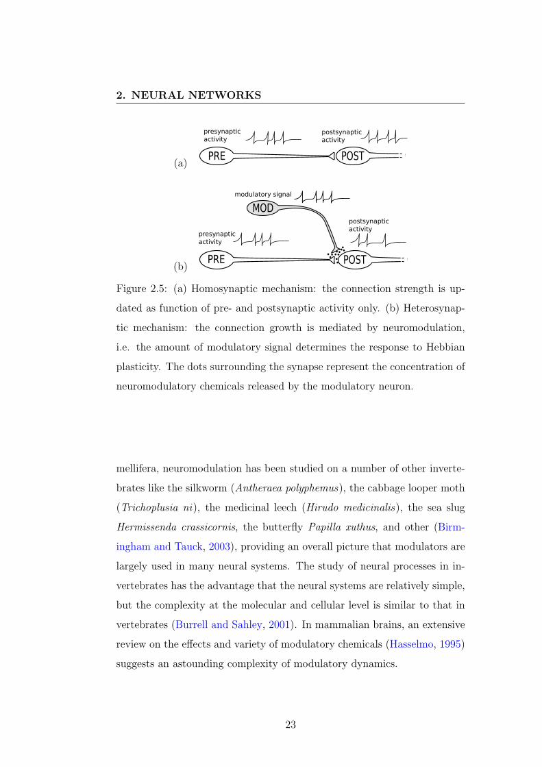
Figure 2.5: (a) Homosynaptic mechanism: the connection strength is up-
dated as function of pre- and postsynaptic activity only. (b) Heterosynap-
tic mechanism: the connection growth is mediated by neuromodulation,
i.e. the amount of modulatory signal determines the response to Hebbian
plasticity. The dots surrounding the synapse represent the concentration of
neuromodulatory chemicals released by the modulatory neuron.
mellifera, neuromodulation has been studied on a number of other inverte-
brates like the silkworm (Antheraea polyphemus), the cabbage looper moth
(Trichoplusia ni), the medicinal leech (Hirudo medicinalis), the sea slug
Hermissenda crassicornis, the butterfly Papilla xuthus, and other (Birm-
ingham and Tauck, 2003), providing an overall picture that modulators are
largely used in many neural systems. The study of neural processes in in-
vertebrates has the advantage that the neural systems are relatively simple,
but the complexity at the molecular and cellular level is similar to that in
vertebrates (Burrell and Sahley, 2001). In mammalian brains, an extensive
review on the effects and variety of modulatory chemicals (Hasselmo, 1995)
suggests an astounding complexity of modulatory dynamics.
23

2. NEURAL NETWORKS
2.1.3.1 Plasticity: Homo- and Heterosynaptic,Associative and non-Associative
Homosynaptic plasticity refers to conditions when the synaptic strength
changes as a function of activities in the pre- and postsynaptic neurons:
two neurons are involved in the process and the connection between them
undergoes changes. The Hebb’s postulate states that the synaptic strength
is increased when the activities of pre- and postsynaptic neurons are closely
correlated in time. For this reason, Hebbian plasticity is labelled associative.
The connection strength between two neurons can also change indepen-
dently of pre- and postsynaptic activities, but as a function of a third mod-
ulatory neuron (Kandel and Tauc, 1965). If a modulatory neuron releases a
modulatory chemical at the synapse cleft, causing synaptic facilitation, the
effect is named heterosynaptic modulation (Bailey et al., 2000). A graph-
ical representation is provided in Figure 2.5. Heterosynaptic modulation
has been observed to lead to synaptic facilitation in the absence of pre- or
postsynaptic activities (Bailey et al., 2000). In such conditions, plasticity
is named non-associative or pure heterosynaptic.
Homo- and heterosynaptic plasticity are closely related by their com-
bined effect. A significant finding is that when heterosynaptic modulation is
coupled with homosynaptic activity, the overall effect is more than additive,
i.e. the effect is more than the sum of each effect separately. This results in
a long term synaptic facilitation. Figure 2.6 illustrates the idea graphically.
These dynamics appear to derive from the activation of transcription factors
(e.g. CREB) and protein synthesis when modulation is coupled with ho-
mosynaptic facilitation, in turn leading to durable and more stable synaptic
configurations. The underlying idea is that the synaptic growth that occurs
in the presence of modulatory chemicals has a substantially longer decay
24

2. NEURAL NETWORKS
than the same growth in absence of modulation.
25

2. NEURAL NETWORKS
(a) Homosynaptic activation4 trains
0 h
1 h
24 h
0 h
1 h
24 h
(b) A single heterosynaptic stimulus
1 x 5-HT
0
10 m
24 h
0
1 h
24 h
(c) Pairing homosynaptic activation with heterosynaptic modulation
1 x 5-HT
0
12 h
24 h
0
12 h
24 h
1 train
Figure 2.6: Non-additive interaction of homo- and heterosynaptic plastic-
ity. The figures were redrawn after the graphical representations in (Bailey
et al., 2000). (a) Short term homosynaptic facilitation is observed at both
bifurcated cultures when a train of spikes is applied to the presynaptic neu-
ron. (b) The application of 5-HT produces short term facilitation of that
synapse. (c) The pairing of homo- and heterosynaptic stimulation produces
a long term facilitation that is greater than the sum of each stimulation
separately. See (Bailey et al., 2000) for further detail.
26

2. NEURAL NETWORKS
2.2 Neural Models
Biological neural networks have inspired the formulation of computational
models, generally referred to as Artificial Neural Networks (ANNs) with
novel computational properties (Haykin, 1999). Neural models and ANNs
have a simpler dynamics than biological neurons and networks. Often the
biological plausibility is not a prime criterion, especially when the main ob-
jective is the achievement of new computational techniques and tools for
engineering. However, the modelling of biological mechanisms is an impor-
tant research field where the biological plausibility is a fundamental aspect
(Bugmann, 1997; Nenadic and Ghosh, 2001a,b; Izhikevich, 2003, 2007b).
Normally, the neuron model is considered the fundamental unit from
which networks can be built as connected graphs. Usually, nodes are in-
stances of the same neuron model. Figure 2.7 represents a connected graph
where the units emulate biological neurons, and the arcs represent connec-
tions between dendrites and axons. A directed graph represents an ex-
tremely high level of abstraction of a neural network because it does not
account for many physical and physiological properties of a three dimen-
sional biological network. In other fields such as computational neuroscience
(Dayan and Abbott, 2001) statistical tools are often used to analyse neu-
ral activities, whereas studies in computational embryogeny (Stanley and
Miikkulainen, 2003b; Federici, 2005a) often represent networks in a two or
three dimensional space. However, ANNs have developed initially from sim-
ple models as the single neuron (or perceptron) and basic architectures. For
this reason, the classification of artificial models often follows the historical
progress.
27

2. NEURAL NETWORKS
N
N
N
N
N
N
N
N
N
Input Hidden Output
Figure 2.7: A graph representing an artificial neural network. Nodes can be
distinguished in three categories: inputs, hidden nodes and outputs. Inputs
nodes are afferent nodes whose activities represent a measure of sensory
units. Outputs produce signals that can be used for decision making, motor
control, etc., similarly to efferent neurons.
2.2.1 Neuron Models
2.2.1.1 Rate-based Models
Biological neurons communicate by propagating action potentials that have
a brief duration and are sometimes referred to as spikes or pulses. In basic
computational models, instead of propagating spikes, the output of a neuron
represents the spiking frequency or rate. For this reason, these models are
called rate-based. In the simplest form of neuron, the output is given by a
function transformation of the weighted inputs:
o = f(a) = f
( n∑i=1
wi · xi
), (2.1)
where x are the values of the inputs and w are the weights of the afferent
connections of the neuron. The value inside the brackets is commonly called
activation (noted here with a). Figure 2.8 shows the graphs of common
28

2. NEURAL NETWORKS
−10 −8 −6 −4 −2 0 2 4 6 8 10−20
−10
0
10
20
Activation
Out
put
−10 −8 −6 −4 −2 0 2 4 6 8 10−0.2
0
0.2
0.4
0.6
0.8
1
Activation
Out
put
(a) (b)
−10 −8 −6 −4 −2 0 2 4 6 8 10−0.2
0
0.2
0.4
0.6
0.8
1
Activation
Out
put
−10 −8 −6 −4 −2 0 2 4 6 8 10
−1
−0.5
0
0.5
1
Activation
Out
put
(c) (d)
Figure 2.8: Functions for neuron output. (a) linear function; (b) step func-
tion; (c) logistic or sigmoid function; (d) Hyperbolic tangent function.
functions used for the neuron output. The step function (Figure 2.8(b)) is
defined as
output =
1 , if a ≥ 00 , otherwise.
(2.2)
The sigmoid function (Figure 2.8(c)) is
output = σ(a) =
1
1 + e−a(2.3)
and the hyperbolic tangent (Figure 2.8(d)) is
output = tanh(a) =e2a − 1
e2a + 1(2.4)
The hyperbolic tangent can also be obtained from the sigmoid as tanh(a) =
2σ(a/2)− 1.
2.2.1.2 Leaky Integrators
For certain problems where the temporal dynamics is not relevant (e.g.
classification problems), feed-forward networks propagate the signals from
input to output where the outcome is read. On the contrary, when temporal
29

2. NEURAL NETWORKS
dynamics play an important role, for example in robotic control and control
systems, it is assumed that certain intervals of time occur between the
moment an input is received and the moment this signal is processed to the
output. Such feature is essential when recurrent connections are present in
the network. In this case, it can be assumed that
a(t) =n∑
i=1
wi · xi(t− 1) , (2.5)
where t is an integer representing the time in a discretised system. At each
time step, the activation of the neuron – and consequently the output – is
a function of the input values x of the previous time step.
In a more accurate model, the activation value can also follow a leaky-
integrator dynamics when its state varies gradually and continuously with
time. In other words, in leaky-integrator models the activation has a value
of inertia. Assuming a small sampling time step ∆t, the activation can be
computed as
a(t+ ∆t) = a(t) +∆t
τ ∗
[ n∑i=1
(wi · xi(t)
)− a(t)
], (2.6)
where τ ∗ is a time constant that determines the speed of update. In contin-
uous time, the variation of the activation a is expressed by the differential
equation
τda
dt=[− a+
n∑i=1
wixi
]. (2.7)
Equation 2.7 was used to describe the dynamics of network nodes in (Pearl-
mutter, 1990; Beer and Gallagher, 1992). Those networks, when imple-
mented with recurrent connections, were called Continuous Time Recurrent
Neural Networks (CTRNN) (Yamauchi and Beer, 1994).
With a sufficiently small time step, Equation 2.6 can be used to integrate
Equation 2.7 as in the example reported in (Blynel and Floreano, 2003)
30

2. NEURAL NETWORKS
where a time step of 1 was used in combination with time constant τ ∗ in
the interval [1,70]. Other similar examples are in (Paine and Tani, 2004,
2005; Tuci et al., 2005; Vickerstaff and Di Paolo, 2005).
When a longer time constant is used, Equation 2.6 results in a slower
modification of the activation value. In a network composed by neurons with
different time constants, some neurons will be more reactive to changes in
the inputs, others will modify their activations more slowly, displaying an
inertia-like dynamics. Because this neuron computes the activation value
as a linear combination of the new inputs and the old activation, it is said
to have memory of the previous states. This kind of network has been used
successfully for many robotics tasks such as obstacle avoidance and navi-
gation, maze navigation and sequential tasks where the temporal dynamics
are important (Blynel and Floreano, 2003; Paine and Tani, 2004, 2005; Tuci
et al., 2005; Vickerstaff and Di Paolo, 2005).
2.2.1.3 Spiking Neurons
Spiking Neural Networks (SNNs), also referred to as pulsed neural networks
(Maass and Bishop, 1999), are so called because they try to model the
pulsed nature of action potentials in biological neurons. At a high level
of abstraction, the neuron state can be implemented as a leaky integrator
that accumulates the charges given by the inputs, but also discharges itself
with time. Equations 2.6 and 2.7 can be used to compute the activation.
When the activation crosses a given threshold value, the neuron “fires” a
spike that is transmitted along the axon. After a spike has been fired, the
activation drops to a low value and the neuron is not able to send another
spike for a certain amount of time called refractory period.
SNNs have more complex temporal dynamics that could be beneficial
when the precise time of firing is relevant (Maass and Bishop, 1999; Wil-
31

2. NEURAL NETWORKS
son, 1999). The simulation of SNNs can be used to model and understand
the spiking dynamics of biological neural systems (Rabinovich et al., 1997;
O’Reilly, 1998; Nenadic and Ghosh, 2001a; Izhikevich, 2003, 2004). Wilson
(1999) defines “spikes, decision and actions” as the dynamical foundations
of neuroscience. Models of spiking neurons also match the properties of
analogue VLSI circuits that can be built on small surfaces and have very
small power consumption. Models have been investigated with the final or
proposed target of hardware implementation (Christodoulou et al., 2002;
Eriksson et al., 2003; Moreno et al., 2005; Upegui et al., 2005).
The use of SNNs in robotics and control systems has also been tested.
Several models of SNNs have been experimented on simulated and real
robots (Floreano and Mattiussi, 2001; Floreano et al., 2004; Zufferey and
Floreano, 2004; Srinivasan and Zhang, 2004; Chahl et al., 2004; Federici,
2005a). However, the precise advantages of using SNNs over traditional
ANNs are not always easy to identify.
2.2.2 Neural Architectures
Despite the complexity of biological neural circuitry, the limitations of de-
sign techniques in ANNs do not allow for the synthesis of similarly com-
plex topologies. Network architectures are generally divided in two main
categories, feed-forward networks and recurrent networks (Haykin, 1999).
Feed-forward networks propagate the signals in one direction only, from the
input to the output as in the example in Figure 2.7. On the contrary, re-
current networks have no constraints on the connectivity and neurons can
have cyclic and self connections as illustrated in Figure 2.9(a).
Traditionally, feed-forward networks have been used for a variety of tasks
including classification, system identification, prediction (Pham and Liu,
1995), and robotic control (Zalzala and Morris, 1996; Omidvar and van der
32

2. NEURAL NETWORKS
N
N
N
N
N
N
N
N
N
Input Hidden Output
N N N N
N N N
NN
Input
Hidden
Output
NNN
memory
units
(a) (b)
N N N
N N NOutput
N
N
N
A
N
N
NN
N
N
B C
Input N N N
N
N
N
Output
N
N
N
High level
controlN
N
N
N
Low level
controlN
Input
(c) (d)
Figure 2.9: (a) In a recurrent neural network, connections can be established
from and to each node. (b) An Elman network is a feed-forward structure
with the addition of memory units that connect to the inner layer with
recurrent connections. (c) Schematic illustration of a modular network with
three modules A, B, and C. (d) Schematic illustration of a hierarchical
network.
33

2. NEURAL NETWORKS
Smagt, 1997). Their use is suitable for nonlinear systems where a complex
mapping between inputs and output is required. When ANNs are employed
as control systems in complex environments and tasks with temporal dy-
namics, recurrent networks are preferred. Recurrent networks are used to
establish cycles among neurons with the property of retaining information in
time. Memory units implemented with recurrent connections often provide
a behavioural advantage in several tasks like navigation, exploration and
foraging (Floreano and Mondada, 1996). Often the term recurrent may not
indicate a particular topology, but rather an unconstrained neural topology
where any connection is allowed.
Elman networks (Figure 2.9(b)) are hybrid topologies that insert a num-
ber of memory unit (with recurrent connections) in a feed-forward structure
(Elman, 1990). In this way a feed-forward network can be enhanced to dis-
play temporal dynamics.
The idea that different neural functions can have a common computa-
tion led to the concept of modularity (Happel and Murre, 1994; Gruau,
1994). In a modular network, similar structures or modules are repeated
with small variations or different connectivity to expand the capabilities of
the network. From an evolutionary and developmental perspective, modu-
larity is considered to have brought about important computational advan-
tages (Bullinaria, 2007). Figure 2.9(c) illustrates graphically the concept of
modularity.
In robotic control, a widespread notion is that of levels of control. The
idea is that a complex control policy is a combination of more dynamics,
some at lower levels, some at higher levels (Brooks, 1986). For instance, the
act of walking can be considered a low level control activity that involves
the activations a series of muscles to maintain equilibrium and a forward
movement. On the other hand, to walk to the nearest source of food is a
34

2. NEURAL NETWORKS
higher level control activity that involves cognitive abilities such as motiva-
tion and planning. Low levels of control, such as walking, are necessary to
achieve higher level control tasks, such as walking to a specific destination.
For this reason, higher levels of control are believed to act on the lower levels
on a hierarchical fashion for example by biasing, regulating or modulating
the low levels. Figure 2.9(d) shows the scheme of a hierarchical network2.
Control networks were evolved in (Paine and Tani, 2005) to perform both
obstacle avoidance and goal seeking behaviour showing that hierarchical
networks performed better than uniformly connected networks.
A variety of other network architectures have been presented in the
literature, e.g. critic-actor structures, scale-free networks and small world
networks.
2.2.3 Learning and Plasticity
The connection weights between the nodes in a network can be either fixed
or varying during operation. If weights change during execution, those
are said to be plastic. The mechanism according to which the weights
are updated is called plasticity rule and can be inspired – although not
2It is important to note that in the network in Figure 2.9(c), the module A pre-
processes information, and consequently feeds modules B and C with its output. The
fact that the module A precedes B and C in the order the information is processed does
not mean that the network is hierarchical. On the contrary, in the network of Figure
2.9(d), both sub-parts of the network are fed by the same input: however, while the
lower part feeds the output and acts directly on the motors, the upper part does not act
directly on the motors, but rather influences the lower part. The information processing
of this latter network resembles most the concept of hierarchical structure. Nevertheless,
given the different interpretations of the word hierarchy, the classification is intended to
be loose.
35

2. NEURAL NETWORKS
necessarily – by plasticity processes observed in biological neural networks.
A plasticity rule is expressed as
dw
dt= g(p(t)
), (2.8)
where g(·) is an arbitrary function of a vector of values p(t). The weight
update can be a function of a variety of values like the activity of the nodes
linked by a connection weight, other signals specific to one or more neurons
in the network, global signals, etc.
Traditionally, functions that update weights according to a global mea-
sure of error in a given task fall into the category of supervised learning
algorithms (Haykin, 1999), and are called learning rules. In this case, the
weight change is viewed as a procedure to minimise an error, giving to the
overall process the resemblance of learning. On the contrary, in control tasks
with temporal dynamics, weight strengths may change continuously with-
out the presence of an explicit error function. In this second case, a weight
update may be based on local values like neural activities of neighbour-
ing nodes. Connections may update continuously their strength in order
to achieve, for example, a cycling dynamics for a central pattern generator
(CPG). This results in a complex temporal dynamics of changing weights
and activations without any external or internal error signal, but solely for
the purpose of achieving certain neural dynamics and overall behaviour.
In this view, the concept of plasticity rule is different from that of learning
rule. Moreover, whether synaptic plasticity leads in some cases to an overall
learning-like behaviour depends also on a series of system level properties
and neural topologies.
Unfortunately, learning-like behaviour, or simply learning is a difficult
concept to define. In (OED, 1989), learning is defined as the act of acquiring
knowledge of (a subject) or skill in (an art, etc.) as a result of a study, ex-
36

2. NEURAL NETWORKS
perience, or teaching. In scientific contexts, learning is usually categorised
and better defined. Simple forms of learning include nonassociative learning
as habituation and sensitisation, associative learning includes classical and
operant conditioning, and the literature presents a large variety of higher
forms of learning (Gallistel, 1993; Britannica, 2007a). Even a short overview
of learning theory is beyond the scope of this thesis. As a consequence, the
use of terms like learning that are inevitably imbued with popular an subjec-
tive acceptations often leads to misinterpretations and ineffectual disputes.
To avoid confusion, although the term learning will be used in general con-
texts, in this thesis the term plasticity rule will be used instead of learning
rule to indicate a mechanism of weight update. Similarly, the term Hebbian
plasticity will be used instead of Hebbian learning.
2.2.3.1 Hebbian Plasticity
An important plasticity mechanism derived from Donald Hebb’s postulate
(Hebb, 1949; Cooper, 2005; Dayan and Abbott, 2001) updates a weight
connection when the pre- and postsynaptic neuron are active at the same
time:
τdw
dt= uv , (2.9)
where w is the connection weight, τ is a time constant that determines the
rate of update, u and v are positive firing rates of the pre- and postsynaptic
neurons. Accordingly, a weight is strengthened when both pre- and postsy-
naptic neurons are active simultaneously. An extension of Equation 2.9 –
which permits only increments – allows also for the decrease of the weight
w by introducing threshold values θu and θv:
τdw
dt= (u− θu)(v − θv) , (2.10)
37

2. NEURAL NETWORKS
Equations 2.9 and 2.10 lead to unstable weights because of the positive
feedback between weight strength and synaptic activities. An alternative
stable rule is the BCM rule (from the inventors Bienenstock, Cooper and
Munro)
dw
dt= η[v2u− θiv]
∆θi = α · [v2 − θi] (2.11)
that utilises a sliding threshold θ to stabilise weights and implement synap-
tic competition; α is the update rate for θ and should be greater than η
(Bienenstock et al., 1982; Dayan and Abbott, 2001).
The Oja rule (Oja, 1982; Dayan and Abbott, 2001)
dw
dt= η[uv − v2w] (2.12)
limits the weight update by subtracting a factor proportional to the weight
itself times the square of the postsynaptic activation.
2.2.3.2 Other Rules: Presynaptic, Postsynaptic and Decay
Synaptic weights can be updated solely on the activity of the pre- or post-
synaptic neuron:
τdw
dt= u− θ (2.13)
τdw
dt= v − θ (2.14)
τdw
dt= k . (2.15)
Although a growing experimental evidence in biology suggests that pre-
and postsynaptic activities alone can modify synaptic connections3, com-
putational models that employ Equations 2.13-2.15 have not been well in-
vestigated. Later in this thesis, it will be shown that pre- or postsynaptic
3For example in habituation or sensitisation (Bailey et al., 2000).
38

2. NEURAL NETWORKS
plasticity alone can lead to adaptivity and useful functions in computational
models.
A linear combination of a correlation-based rule (Equation 2.9), a presy-
naptic rule, a postsynaptic rule and a decay rule (Equations 2.13, 2.14, and
2.15) was employed in (Montague et al., 1995; Niv et al., 2002). Pre-, post-
synaptic and covariance rules (Equation 2.10) were employed in robotic
navigation tasks in (Floreano and Urzelai, 2001b,a; Urzelai and Floreano,
2001; Nolfi and Floreano, 2002; Blynel and Floreano, 2003). Similar plas-
ticity rules have been implemented for spiking neurons in the form of spike
timing dependent plasticity (STDP)(Roth et al., 1997; Nielsen and Lund,
2003; Federici, 2005a), or other models (Kitajima and Hara, 2000).
2.2.3.3 Computational Models of Neuromodulation
Computational models of neuromodulation can be used to test features on
functional tasks or problem solving, often resulting in a better identification
of the advantages of neuromodulation. Simulated or real robotic controllers
enhanced by neuromodulation and tested in closed-loop conditions can also
suggest similarities between ways of functioning in artificial and biological
controllers. Ultimately, as the role of neuromodulation has not been entirely
clarified in biology, computational and robotics models address tentatively
problems over a large scope in order to identify relations between the fea-
tures of the model and its performance in certain tasks. Neuromodulation
can be employed for a variety of purposes like for implementing CPG, fil-
tering or regulating sensory and motor processes, and achieving adaptation,
learning and memory.
39

2. NEURAL NETWORKS
2.2.3.3.1 Classification. The variety of modulatory effects in biology
have resulted in diverse approaches to computational models. In order
to overview the field, a classification was introduced in the review paper
(Fellous and Linster, 1998), where different features of neuromodulation
were identified and used for categorising existing studies.
It is important to note that categories are not precisely defined, nor
describe accurately the multifarious modulatory effects observed in biology
whose dynamics are still mostly unknown. However, such classification helps
to describe a large variety of different studies in the relatively young field
of computational models of neuromodulation.
Extrinsic and intrinsic modulations refer to the spatial origin of modu-
latory signals. If those are generated outside the neural circuit responsible
for a given computation, modulation is said to be extrinsic. If modulation
is generated inside the circuit being modulated, it is said to be intrinsic
(Katz, 1995). Extrinsic modulation is considered a way of altering the
computational characteristics of a target circuit, but does not sustain the
computation itself. On the other hand, intrinsic modulation is a working
mechanism to achieve specific neural dynamics in a self-contained compu-
tational unit (Katz and Frost, 1996).
Regulatory modulation, generally associated with intrinsic modulation,
refers to the regulatory action that governs a given neural computation.
Therefore, regulatory modulation is essential for the neural computation.
On the other hand, when modulation is decoupled from the network and
its computation, modulation has a tuning function consisting in adjusting
over time parameters or ways of functioning.
The time scale of modulatory dynamics can be classified in two possible
cases 1) fast computations, slow modulation and 2) slow computations, fast
modulation. Most studies consider modulation on a longer time scale dy-
40

2. NEURAL NETWORKS
namics than neural computation. In this case, modulation has the function
of adapting the network behaviour in the medium and long term, for exam-
ple adjusting the neural controller to environmental conditions such as light
and darkness. In other cases, fast modulation can act on slow computa-
tion. This is the situation when modulation encodes environmental cues or
events. For example, a very brief but important reward signal can modulate
a longer-term learning process. For a detailed description of the categories
mentioned above refer to (Fellous and Linster, 1998).
Finally, neuromodulation can act on neural processes as a gating signal
of different nature. These processes can be ion currents, rates of chemical
diffusion, modulation of higher level parameters for plasticity, neural trans-
fer functions, etc. Given the generality of the term neuromodulation, it was
essential for a proper classification and understanding of the work in this
thesis to introduce a classification based on the process being modulated.
At a high level of abstraction, modulatory signals can serve for
1. modulation of synaptic efficacy;
2. modulation of neural properties like spiking modes or rates, or output
transfer functions;
3. modulation of rates in synaptic plasticity;
4. modulation of higher levels of plasticity (metaplasticity) or growing
self-organising networks.
The first case indicates that modulation is used to adjust the efficacy of
diffuse or specific synapses, altering or filtering signal propagation at dif-
fuse or specific sites. This can be useful when a mechanism is required to
enhance or suppress stimuli from different inputs, neural areas, or modulate
41

2. NEURAL NETWORKS
motor actions. The second case refers to the modulation of properties of the
neural cell, for example enhancing or suppressing the firing rate, changing
the firing mode or threshold, or the output function. This can be useful to
change working modes of a network (e.g. regulating slow or fast walking in
a robot). The third situation is when modulation applies a gating effect on
plasticity rates. This case, inspired by heterosynaptic plasticity and there-
fore defined neuromodulated plasticity, is used to modify the plasticity rate
at diffuse or specific areas of the neural circuit. This is the type of neuromod-
ulation studied in this thesis. Finally, whereas normally neuromodulation
acts on existing neurons and connections, modulation of growing processes
and metaplasticity (point 4) deal with more substantial changes in the net-
work topology for example growing or pruning connections in developmen-
tal phases, or radically changing the plasticity mechanism (metaplasticity)
(Abraham and Bear, 1996).
Several computational models spanning over the above categories have
been proposed in the literature particularly in the last two decades. An
overview of studies that relate to the work in this thesis is presented fol-
lowing. Given the large scope and variety of approaches, from theoretical
computation to simulated controllers and real robots, the literature presents
scattered examples of modulatory networks that are often difficult to de-
scribe in an homogeneous picture.
2.2.3.3.2 Aplysia and other invertebrates. An important category
of studies was inspired by neural systems of invertebrates, and in particular
the mollusc Aplysia whose neural dynamics were initially studied in (Kan-
del and Tauc, 1965; Carew et al., 1981). An accurate modelling of a sensory
neurons modulated by serotonin in Aplysia is presented in (Baxter et al.,
1999). In (Deodhar and Kupfermann, 2000), genetic algorithms were used
42

2. NEURAL NETWORKS
to optimise the parameters of a two-neuron system that simulated muscu-
lar oscillations during feeding in Aplysia. In (Birmingham, 2001), sensor
flexibility in the crustacean stomatogastric nervous system is observed to
be enhanced by neuromodulation, and it is suggested that analogue mech-
anisms can be used in artificial motor control systems.
2.2.3.3.3 Role of dopamine. Worthy of a particular note are the nu-
merous studies on the role of dopamine. After dopaminergic neurons were
discovered to encode prediction errors and reward information in monkey’s
brains (Schultz et al., 1993, 1997), a number of studies focused on com-
putational models of dopaminergic systems. A model for dopamine using
predictive Hebbian learning was proposed in (Montague et al., 1996). Sim-
ilarities between dopaminergic activities and temporal difference signals in
reinforcement learning (Sutton and Barto, 1998) were outlined in (Suri,
2002; Dayan and Balleine, 2002; Niv et al., 2005), whereas the computa-
tional implications of dopamine in behaviour control and neural disorders
are suggested in (Fellous and Suri, 2002; Montague et al., 2004). In (Suri and
Schultz, 1999), a neural network with a dopamine-like reinforcement learn-
ing was designed based on a temporal difference model with an actor-critic
architecture (Sutton and Barto, 1998) showing a similar learning dynamics
to those recorded in monkeys’ brains (Schultz et al., 1993). An actor-critic
model of reinforcement learning was also used in (Khamassi et al., 2005) to
simulate reward-seeking behaviour with four pre-designed neural architec-
tures. The function of dopamine has been further modelled in the striatum
(Suri et al., 2001), in the prefrontal cortex (Dreher and Burnod, 2002) and
in basal ganglia (Gruber et al., 2006).
Given the important effect of dopamine at the system and behavioural
level, studies on such neuromodulators allowed for the formulation of hy-
43

2. NEURAL NETWORKS
potheses on the neural bases of decisions in humans (Holroyd and Coles,
2002; Daw et al., 2006; Li et al., 2006; Cohen, 2008). At a similar level,
attempts to model emotions with neuromodulatory dynamics have been re-
viewed in (Parussel, 2006; Levine, 2007). Extending the analysis to other
modulatory chemicals, Doya (2002) suggested a framework where dopamine
signals the error in reward prediction, serotonin controls the time scale of re-
ward prediction, noradrenaline controls the randomness in action selection,
and acetylcholine controls the speed of memory update. As pointed out
in (Decker and McGaugh, 1991; Bacciottini et al., 2001), important neural
dynamics might emerge from the interaction of more modulatory systems.
2.2.3.3.4 The gap between cellular and system levels. Many be-
havioural and system level studies do not explain the cellular mechanisms
that causes the higher level dynamics to emerge. If the final tasks is to re-
produce the features and dynamics of neural systems, the knowledge of the
basic cellular mechanisms is essential to the implementation of a complex
system in the whole. The missing link between synaptic mechanisms and
behavioural control has been outlined in (Harris-Warrick and Marder, 1991)
and following in the review papers (Destexhe and Marder, 2004) and (Dub-
nau et al., 2002) where memory mechanisms are described to emerge from
synapse to system. Moreover, reinforcement learning theories and machine
learning approaches do not account for many computational processes in
the brain (Kawato and Samejima, 2007). As a consequence, studies on the
basic synaptic mechanisms of modulation are important bottom-up inves-
tigations.
2.2.3.3.5 Bottom-up studies. The optimisation of plasticity rules that
apply on synapses and are based on associative local measures like the Heb-
44

2. NEURAL NETWORKS
bian principle was proposed in (Bengio et al., 1992). Abbott (1990) pro-
posed a model of heterosynaptic plasticity to implement a memory mech-
anism for initiating and terminating learning in networks. The model in-
troduced neuromodulation as a multiplicative factor on synaptic plastic-
ity. With a similar multiplication operation, a recent study (Porr and
Worgotter, 2007b) defines the modulatory signal – the signal that enables
learning – as the third multiplication factor to associate two stimuli. The
third factor is shown to enable learning when auto-correlation of stimuli is
minimal and cross-correlation is maximal, allowing for a stabilisation of con-
nection strengths. Short-term memory with modulated plasticity was inves-
tigated in (Ziemke and Thieme, 2002) where a robot navigated in a T-maze
and remembered turning directions according to visual clues in the maze.
The feed-forward control networks had a decision unit that propagated a re-
current signal to update connection weights. Learning and adaptivity were
shown in navigation tasks in (Sporns and Alexander, 2002). In (French
and Canamero, 2005), neuromodulation was implemented on a Braitenberg
vehicle (Braitenberg, 1984) to achieve adaptation. Walking behaviour in a
quadruped robot (Fujii et al., 2002) was synthesised using four types of ge-
netically determined neuromodulators to drive a central pattern generator
(CPG). In (Kondo, 2007), an evolutionary design and behaviour analysis of
feed-forward networks with neuromodulators was proposed to fill the gap
between simulation and real robotic control. Improved evolvability in neural
controllers was shown with the use of GasNet (Smith et al., 2002b), where
modulation is co-transmitted with standard activation signals and results
in gating the steepness of the logistic output function of neurons.
2.2.3.3.6 Plasticity for reward-based learning. In some testing en-
vironments, a particular importance is given to reward signals that indicate
45

2. NEURAL NETWORKS
to the neural controller the occurrence of a favourable situation, item or
action. Dynamic, reward-based scenarios are environments where reward
items dynamically change location or change the course of actions by which
they can be obtained. Such situations require highly adaptive and learn-
ing behaviour to enable an agent to adjust its strategies during lifetime.
Moreover, reward signals are timed and specific, often requiring a compu-
tation that can differ considerably from other sensory information. Many
of the studies on the role of dopamine described above investigate reward-
based learning. Currently, reward-based learning is often investigated at
the system level dynamics, describing global learning signals as prediction
errors and temporal difference (TD) (Sutton and Barto, 1998). A problem
when modelling classical and instrumental conditioning is to understand the
mechanisms that allow for linking stimuli occurring at different times. The
problem is named the credit assignment problem or distal reward problem
(Izhikevich, 2007a; Nitz et al., 2007; Farries and Fairhall, 2007).
It is important to note that the process by which conditioned stimuli
and unconditioned stimuli or rewards are associated can be classified as
system level dynamics, and although such dynamics emerge possibly from
local synaptic plasticity mechanisms, it is not straight forward to under-
stand the relation that links synapse to system (Worgotter and Porr, 2005).
In this attempt, a top-down approach consists in describing the system level
(or learning) dynamics, and consequently searching for plasticity rules that
allow for the generation of the target dynamics. Alternatively, bottom-up
approaches consist in the identification of candidate plasticity rules (upon
the supposition that those could be the basis of the dynamics being sought),
and attempt the construction of system level dynamics from those. The
work in this thesis can be classified as bottom-up and belongs to the cat-
egory of studies where instrumental learning was achieved without explicit
46

2. NEURAL NETWORKS
representation of prediction errors or temporal difference signals. Belonging
to this category, a study in (Montague et al., 1995) employs a multiplicative
modulatory effect similar to that in (Abbott, 1990) to simulate reward-based
learning in a foraging bee. The model was inspired by the activity of the
neuron VUMmx1 in the honey bee that carries gustatory stimuli. A similar
model was later used in (Niv et al., 2002) in combination with a genetic
algorithm to optimise a learning rule and weights in a one-neuron network
for the same bee foraging problem.
47

Chapter 3
Phylogenetic Search
Artificial evolution is a stochastic search that draws inspiration from the
Darwinian principle of natural selection (Darwin, 1859). Artificial evolu-
tion is a simulated evolutionary process that takes advantage of recent ad-
vances in technology and computation tools. The process is described by
algorithms commonly referred to as Evolutionary Algorithms (EAs). Evolu-
tionary Algorithms have become an important tool in many research fields
with a multitude of applications in optimisation, design, engineering and
other.
3.1 Motivations
Evolutionary Algorithms are flexible search algorithms whose primary pur-
pose can vary considerably and can be adjusted to diverse tasks. Three
mainstreams in the use of EAs can be outlined here.
(1) EAs are often applied as optimisation techniques to difficult prob-
lems where the search space does not allow for exhaustive search or where
good techniques or heuristics have not been established yet. The increased
knowledge and expertise on the use of EAs during the last decades have
made those algorithms a valid and accepted tool in optimisation. However,
48

3. PHYLOGENETIC SEARCH
the high requirements in computational power and the lack of reliability do
not consent their use on mission-critical and safety-critical applications.
(2) Evolutionary techniques emulate the natural processes that have
concurred to generate the extent and complexity of living creatures on the
Earth. In this view, the focus does not lie exclusively on finding one fi-
nal solution but rather on the evolutionary process itself, and the analogies
between natural and artificial evolution. In a way, it is possible to un-
dertake the study of natural evolution by means of computational tools, or
computational evolution. Relevant research issues focus on the genomic rep-
resentation of solutions and phenotype mapping, the importance of sexual
recombination of genomic information, the effect of modifying the intensity
and modality of selection pressure, the role of diversity in the population
and speciation mechanisms, the size of the population or the effect of dif-
ferent mutation strengths. A large variety of topics, which go beyond the
purpose of this overview, has been addressed by the Evolutionary Compu-
tation community.
(3) A third approach in using evolutionary techniques focuses on the ten-
tative exploration of innovative designs and solutions that can be achieved
by combining new mathematical tools, software or hardware with evolu-
tionary search. This approach does not focus exclusively on a measure of
quality of the final solution, nor exclusively on the dynamics of the search
process, but rather on the combination of the two to generate innovative
features of evolved solutions. This was the approach used in this thesis to
investigate the potential of a new type of neuron whose use and potential
were unknown. Fields of evolutionary computation that endeavour in this
directions are principally Artificial Life, Evolutionary Robotics, Evolvable
Hardware, Generative and Developmental Systems.
49

3. PHYLOGENETIC SEARCH
3.2 Overview of Algorithms for
Artificial Evolution
EAs according to different implementations are named also Evolution Strate-
gies (Back and Schwefel, 1993), Evolutionary Programming (Fogel, 1994),
Genetic Algorithms (Goldberg, 1989) and Genetic Programming (Koza,
1992). Search algorithms that can be commonly classified as Evolution-
ary Algorithms have been applied to a wide variety of problems: numerical
and combinatorial optimisation problems, evolutionary arts and design, en-
gineering design processes and many others. EAs are implemented in a large
variety of different algorithms. The fundamental Darwinian idea of natural
selection that inspired EAs is a compelling but broad concept that involves
a number of particular aspects, each of which can be modelled in various
ways. A general procedural steps however can be outlined.
An EA initiates the search by creating a population of random solutions.
The solutions are then tested to associate a measure of quality to each of
them. Generally, because solutions are randomly created, they return dif-
ferent values of fitness, resulting in some solutions performing better, others
worse. After the evaluation, a selection mechanism is in charge of selecting
a subset of solutions from the whole population. The selection mechanism
is biased to select with higher probability solutions that performed better
on average. These solutions are often named parents because they form
a subset of individuals that are allowed to reproduce. The genotypes of
parents are cloned and mutated in order to generate similar but not identi-
cal solutions. If crossover (or recombination) is implemented, two or more
genotypes are combined to form one or more children. The new solutions
represent a new generation that, descending from a small set of well per-
forming parents, have higher probability of scoring higher fitness than the
50
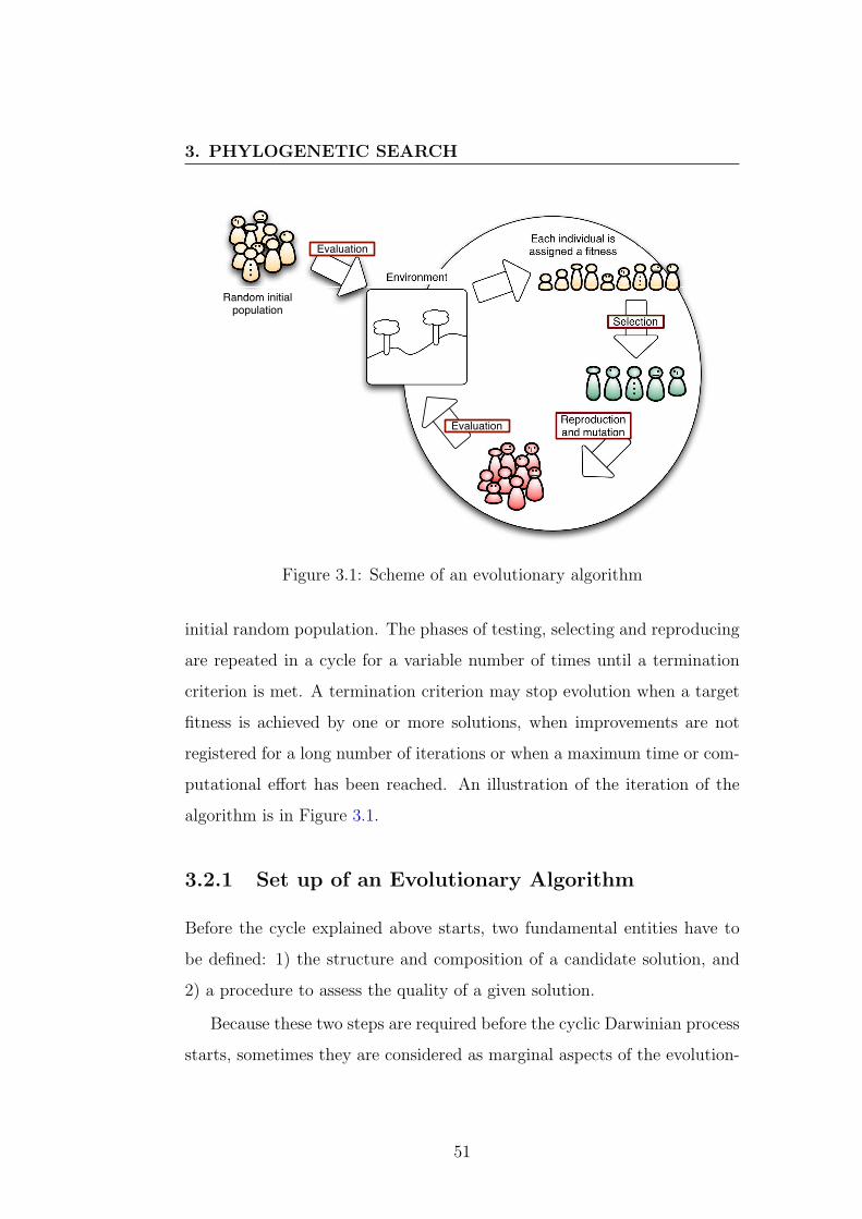
3. PHYLOGENETIC SEARCH
Random initial population
Environment
Each individual is assigned a fitness
Selection
Reproduction and mutation
Evaluation
Evaluation
Figure 3.1: Scheme of an evolutionary algorithm
initial random population. The phases of testing, selecting and reproducing
are repeated in a cycle for a variable number of times until a termination
criterion is met. A termination criterion may stop evolution when a target
fitness is achieved by one or more solutions, when improvements are not
registered for a long number of iterations or when a maximum time or com-
putational effort has been reached. An illustration of the iteration of the
algorithm is in Figure 3.1.
3.2.1 Set up of an Evolutionary Algorithm
Before the cycle explained above starts, two fundamental entities have to
be defined: 1) the structure and composition of a candidate solution, and
2) a procedure to assess the quality of a given solution.
Because these two steps are required before the cyclic Darwinian process
starts, sometimes they are considered as marginal aspects of the evolution-
51

3. PHYLOGENETIC SEARCH
ary search. On the contrary, expertise on the use of EAs indicates that the
correct set up of the algorithm is often more relevant than the evolution-
ary process itself for the achievement of good solutions. Unfortunately, this
view has been unpopular in the past: outlining the importance of the set
up means to lessen the virtue of the algorithm and give back the design
and critical choices in the hands of the engineer, consequently recognising
the limitations of the automatic synthesis and design (Soltoggio, 2004b,c).
A description of issues related to the design of the fitness function is pro-
vided in the following. Topics related to the genotypical and phenotypical
representation will be discussed later in the context of ANNs. For all other
aspects of evolutionary search, refer to the extensive literature in the field
(Goldberg, 1989; Back and Schwefel, 1993; Michalewicz, 1996).
3.2.2 Fitness Design
The design of the fitness function is a fundamental issue to guarantee an effi-
cient search especially in the fields of artificial life and evolutionary robotics.
When EAs are employed for optimisation tasks, they are generally tested on
given analytical test functions. On the other hand, in real world scenarios
the objective to be achieved is not always well formulated. At least three
aspects of the fitness design can be identified: 1) how to describe with a
value the quality of a solution, 2) how to design a fitness landscape that
favours a successful search and 3) how to favour the synthesis of incremen-
tally complex solutions and behaviour.
3.2.2.1 Description of Behaviour
In many problems it is difficult to translate a human concept of well func-
tioning or good performance into a measurable quantity. For example, in
the fields of automation, control and robotics, the expertise of engineers
52

3. PHYLOGENETIC SEARCH
is often required for a good assessment of quality. Unfortunately, an EA
is an automated design procedure that – with the exception of interactive
EAs – does not rely on human interaction during the search process. This
feature, although normally considered a quality, occasionally leads EAs to
produce unfeasible solutions. An example is provided in (Koza et al., 2000)
where a control system designed by Genetic Programming (GP) was shown
to outperform drastically the mathematically optimal PID control system
described in (Bishop and Dorf, 2001). A later analysis in (Soltoggio, 2004a)
revealed that the GP process exploited a flaw in the fitness definition that
allowed the synthesis of a control system with a virtually infinite bandwidth.
These simulated control systems, despite achieving a high fitness according
to the definition in (Koza et al., 2000), are not realisable from a control
engineering viewpoint, see (Soltoggio, 2004a,b,c) for more details.
On the contrary, a successful example of fitness definition is provided
in (Floreano and Mondada, 1994) where a small two-wheeled robot was
controlled by an evolved neural network to perform navigation, obstacle
avoidance and maximise speed in a cyclic path between walls. In this case,
the task of the robot is to navigate or move around quickly without hitting
the walls. Experiments on this kind of two-wheeled robots carried out as
preliminary studies for the work in this thesis revealed that a variety of odd
behaviours might develop to increase a badly defined fitness: for example
a spinning behaviour maximises the wheel speed without danger of hitting
walls, but does not result in a translation of the robot. The fitness suggested
in (Floreano and Mondada, 1994) is the product of three factors: the average
wheel speed, a component indicating straight direction and the distance
from the walls. Currently, this fitness function is still the most appropriate
for this kind of problems.
53

3. PHYLOGENETIC SEARCH
3.2.2.2 Fitness Landscapes
The fitness measure should not just describe the optimal behaviour or qual-
ity, but also many intermediate steps. This is necessary for the progressive
improvement of solutions over the evolutionary process. For example, dur-
ing the early stage of the search, most random solutions will score a very
low fitness and would generally be far from the optimal. However, some
solutions, although poor, will be slightly better and others slightly worse.
The selection mechanism relies on this difference to improve, even slightly,
the average fitness of the population.
A good fitness function should reward good behaviour on a continuous
scale, assigning a positive value of fitness even to small achievements so long
as those achievements could represent an intermediate step to obtain good
solutions. Similarly, if a wrong behaviour can be identified, this should be
punished by decreasing the fitness. However, particular attention should
be given by not exceeding with the punishment of undesired features as
this decreases diversity and eventually hinders the search in ill-behaved
landscape. In landscapes with many local optima, a search based on novelty
of behaviour for a navigation problem showed better results than a fitness-
based evolution (Lehman and Stanley, 2008).
3.2.2.3 Incremental Complex Behaviour
Complex tasks often require a set of incremental skills to be solved. For
example, a robot homing behaviour (a robot explores the environment and
returns to a home location) requires initially the implementation of basic
navigation skills like obstacle avoidance. When basic navigation skills are
acquired, the evolution of exploratory and homing behaviour can take place.
In this type of problem, if the fitness is defined as the number of times the
54
3. PHYLOGENETIC SEARCH
robot reaches the home location over many trials, a boot strap problem oc-
curs when none of the robots achieve the home location, because for instance
none is capable of avoiding obstacles. As a consequence, all individuals in
the population will achieve fitness 0, and the selection mechanism can not
select better individuals.
To avoid this problem, the idea of incremental evolution was introduced
to achieve complex general behaviour (Gomez and Miikkulainen, 1997). In
incremental evolution, two or more separate evolutionary processes are per-
formed in succession to achieve incrementally each level of complexity. In
the previous example of the homing robot, a first evolutionary process would
evolve robots with good obstacle avoidance, and subsequently a second evo-
lutionary run is performed to achieve homing behaviour.
A problem in incremental evolution is that individuals evolved during
the first run might have converged to specific solutions, and those might
not easily evolve to achieve the second complex task: for example, a robot
evolved to avoid obstacles, but only by turning left all the time, whereas
homing requires turning right at times. Another problem might occur if the
individuals in the second run – that are not evaluated on the first skill any
longer – start losing that first skill due to mutations. For example, a walking
robot might evolve homing behaviour, but the walking skill decreases and
eventually the robot reaches home by crawling on the ground.
Often a good design of the fitness function allows for the evolution of
complex behaviour without the need of breaking the evolutionary process
in more phases. This can be achieved by awarding all the necessary skills
for accomplishing the final task. In this way the fitness landscape has a
gradient for each level of complexity.
55

3. PHYLOGENETIC SEARCH
3.2.2.4 Parameter Setting and Search Space
EAs are flexible algorithms that can be applied to a large variety of design
areas and optimisation. However, such flexibility is paid by the effort that
each problem requires in designing, not only the fitness function, but also
the most appropriate settings and search space. Few are the rules, and
the expertise of the engineer often makes the difference. In particular, the
search space has to be somehow measured on the computational effort that
can be employed. Large search spaces consent a larger variety of possible
solutions, and are therefore preferred when novel and unseen solutions are
sought. However, large search spaces can lead to unsuccessful search or poor
performance. Smaller search spaces allow for a faster search, and possibly
result in a easier fitness landscape which lead to successful search and good
final performances. However, a small search space implies inevitably a more
limited search and less novel solutions. A remarkable difference in perfor-
mance was measured in a comparison of a Genetic Algorithm (a small search
space was used) with a Genetic Programming algorithm (with a much larger
search space) in the search and optimisation of control systems (Soltoggio,
2004b).
3.3 Design and Evolution of ANNs
The design of ANNs does not benefit from intuitive procedures or estab-
lished methods. For this reason, evolutionary algorithms have been success-
fully applied in this area as thoroughly overviewed in (Yao, 1999). EAs can
be applied to the design of neural networks at different levels. Basic algo-
rithms perform the optimisation of connection weights in a network graph,
assuming that all other network features are specified, i.e. the number,
types and dynamics of nodes, and other parameters. Other algorithms de-
56

3. PHYLOGENETIC SEARCH
sign both the network topology and the connectivity among nodes. When
neural models include other bio-inspired features, like synaptic plasticity,
evolution can be used to search for plasticity rules and other parameters
regulating various aspect of the networks. Finally, EAs have been applied
to the search of procedures and rules for developmental processes whose
final result is the desired neural network.
The evolution of networks is therefore a multi-fold problem. Looking at
natural processes that lead to the generation of a fully-fledged neural system,
three main areas can be identified: evolution, developmental processes and
environmental adaptation or learning. The design of neural networks can
proceed along one or more of these dimensions. Moreover, the observation
that a neural system (e.g. the human brain) is not created in its adult
mature state, nor it reaches a stable state at all, led the scientific community
to research new design methods for neural systems from the synergy of
development, evolution and adaptation.
3.3.1 Development, Evolution and Adaptation
Living organisms are complex dynamical systems in the way that their ex-
istence is characterised by highly mutable shapes, dimensions and chemical
composition. The advantage of looking at living organisms as dynamic
systems is that the focus lies on the changes that take place according to
certain rules and mechanisms. These rules or mechanisms are in fact what
builds and constructs such systems. If an organism is seen as a mutable
entity, evolution is the process by means of which the instructions rules
were discovered. Development is the complementary process that governs
the formation of a mature phenotype. Multi cellular organisms grow from a
single cell (zygote) that, with reproduction and differentiation, transforms
itself into millions of cells with different function and positions. Finally,
57

3. PHYLOGENETIC SEARCH
Adaptation & Learning
Development
Artificial
Embriogeny
Evolved Adaptive
Developmental
Neural-controllers
Evolved Adaptive
Neural-controllers
Dynamical adaptive
systems
Evolution of
Developmental
Systems
Search
Evolution
Figure 3.2: Phylogenetic, Ontogenetic and Epigenetic space (POE) also
referred to as Evolution, Development and Learning space (Sipper et al.,
1997).
an organism adapts to factors that are not specified in the genotype but
derive from the environment. This process can be seen as a subtle form
of morphogenesis that tunes the organism and its internal mechanisms to
perform best in its own environment. This process is often referred to as
adaptation or learning. These three processes have also been defined Phy-
logeny, Ontogeny and Epigenesis (POE) (Sipper et al., 1997; Moreno et al.,
2005), indicating evolution, development and learning. The POE model has
been used to classify methods and tools for designing biologically inspired
systems, see Figure 3.2. Most of the research so far has focused along one
axis at a time. Approaches that combine two or more processes are in-
evitably more complex but promise to result in more advanced solutions
(Eriksson et al., 2003; Tyrrell et al., 2003; Federici, 2005a,b). The POE
58

3. PHYLOGENETIC SEARCH
paradigms are described separately in the following sections on Encoding
and Development, Evolution and Learning.
3.3.1.1 Encoding and Development
Development can be seen as the procedure by which information in the
genome is used to construct the phenotype. Although this procedure is
independent of evolution, the latter depends heavily on the encoding. For
basic EAs, the process of mapping is a simple one-to-one function where each
feature of the phenotype is directly specified by one gene in the genotype.
This is called direct encoding. The use of a direct encoding has limitations
due to the large search space the derives from specifying all phenotypical
features in the genotype. Direct encoding is used very seldom in any engi-
neering field where complex machines, devices, buildings are not described
by a 3D discrete matrix of chemical composition, but rather by a set of
functional instructions, elements, geometry and properties. Even consider-
ing the suitability of EAs for high dimensional problems, direct encoding
appears not to scale or generalise well.
Artificial Embryogeny (AE) is defined as a sub-discipline of EC in which
phenotypes undergo a developmental phase (Stanley and Miikkulainen, 2003b;
Bowers, 2006). Developmental rules permit the exploitation of regularities
in the phenotype. This form of reuse increases the efficiency in the rep-
resentation. Evolutionary processes that use a developmental phase have
been named “artificial ontogeny”, “computational embryogeny”, “cellular
encoding”. Stanley and Miikkulainen (2003b) use the term Artificial Em-
bryogeny to refer to all the previous. There are two main approaches to arti-
ficial embryogeny: grammatical development (grammatical rewriting called
L-systems) and cell chemistry development (reaction-diffusion models). As
reviewed in (Stanley and Miikkulainen, 2003b), the field of artificial embryo-
59
3. PHYLOGENETIC SEARCH
geny is developing rapidly and tackles a broad set of issues concerned with
the complex dynamics of developmental systems. Despite the relevance of
AE in evolving neural networks, its use implies an increased complexity in
the algorithms. For small search spaces, AE might not result in a significant
advantage.
3.3.1.1.1 Analog Genetic Encoding (AGE)
AGE is a bio-inspired encoding method for network graphs that uses a
direct representation of network nodes and an implicit representation of net-
work weights. Thus, each node in the phenotype is expressed by a distinct
part in the genome, whilst the connections between nodes are derived as
a function of parts of the genotype associated with the nodes: this will be
made clear shortly. The method AGE is fully described in the Ph.D thesis
(Mattiussi, 2005). An overview is given here, further detail can be found in
the literature (Mattiussi, 2005; Mattiussi and Floreano, 2007; Durr et al.,
2006; Marbach et al., 2007).
AGE describes an analog network by means of an artificial genome rep-
resented by an ordered sequence of nucleotides. Nucleotides are expressed
with the characters of an alphabet Ω, for instance the letters A-Z. Nodes
in the network, also called devices, are encoded by particular sequences of
characters, the tokens. Each token signals the presence of a device that is
decoded into a network node in the phenotype. Figure 3.3 shows an example
of a fragment of an AGE genome. Each device has a certain number of in-
puts and outputs that, in the case of neurons, represent dendrites and axon
projections. Inputs and outputs of devices are encoded with terminal se-
quences, i.e. arbitrary sequences of characters that follow device tokens (NE
in the example) and are limited by a terminal token (TE). Once all the net-
work nodes have been extracted, the connections among them are derived.
60

3. PHYLOGENETIC SEARCH
W EN F Y I S T E L C F T E I LI S E N E DNH T E V B T ET Y
tokens
terminal sequences
tokens
terminal sequences
non-coding sequences
PR
Figure 3.3: Fragment of an AGE genome. In this example, the tokens
NE signal the presence of a neuron. The two tokens TE determine the
end of terminal sequences. Terminal sequences are used to determine the
connection weights among devices.
NE
NEF Y I S L C FI S
D V TB
NEK S Z F CY H
Sequence alignments
G EE
Sequence alignments
Sequence alignments
Sequence alignments
R
Figure 3.4: The devices, once extracted from the genome, are connected
with connection strengths that derive from a measure of similarity between
terminal sequences. To connect three neurons, nine alignments are per-
formed.
61

3. PHYLOGENETIC SEARCH
The output terminal sequence of a device is aligned with the input termi-
nal sequences of all other devices; each alignment produces an alignment
score – an index of similarity between the two terminals. This is computed
using a scoring matrix that specifies the score of each couple of nucleotides
when aligned. Examples of scoring matrices are in (Mattiussi, 2005). The
alignment score is consequently mapped into a connection weight. This is
done by pre-setting a number of parameters: for example alignment scores
below 5 result in no connection, alignment scores in the range 6-16 result
in weights with values in the range [1,10], alignment scores higher than 16
result in the maximum weight of 10. Figure 3.4 shows the alignments of the
input and output sequences with three neurons.
3.3.1.2 Evolution
In the POE space, evolution refers to the search algorithm that is applied
to the genome. As described at the beginning of this chapter, evolutionary
search is based on the reproduction and mutation of selected individuals.
In light of this, the evolutionary search is concerned exclusively with the
operations at the genome level and the evaluation of the phenotype. At a
more accurate analysis, natural evolution resulted in the evolution of the
developmental process itself, and studies have shown the strong interac-
tion between evolution and learning (Hinton and Nowlan, 1987; Nolfi, 1999;
Paenke, 2008). For clarity, the evolutionary features will be described sep-
arately from development and learning.
An evolutionary algorithm for neural networks generally includes the
following main features.
• The representation of a population of networks.
• A simulated or physical environment where individuals are tested.
62

3. PHYLOGENETIC SEARCH
• A selection mechanism that chooses networks for reproduction.
• A mutation operator that, either during or immediately after repro-
duction, mutates the genome generating offspring that are an imper-
fect copy of the parents. The mutation strength and the probability
distribution of the noise that generates mutation are important fea-
tures. Adaptive mutation strength is a popular feature implemented
in various evolutionary algorithms such as evolution strategies (ES)
(Back et al., 1997).
• A crossover operator that combines two or more networks to generate
a new offspring.
• A variable length genotype is useful when the number of features
or complexity of the phenotype is not known a priori. A variable
length genotype empowers the evolutionary algorithm with a large
search space. To such purpose, extra genetic operators are introduced:
addition, duplication and deletion that respectively add, duplicate or
remove parts of the genotype.
For each of these features, the literature on Evolutionary Algorithms
and Neural Networks proposes studies over approximately three decades
resulting in a large theoretical and experimental knowledge on the subjects.
The author refers to the literature for further detail (Yao, 1999; Floreano
et al., 2008). The particular aspects of the evolutionary algorithms used in
this thesis will be described and justified later in Chapter 5.
3.3.1.3 Adaptation and Memory
A desired feature in neural networks is often the robustness to environ-
mental changes and the capability of adapting to new scenarios. In this
63

3. PHYLOGENETIC SEARCH
respect, biological networks display remarkable capabilities of adaptation.
In the field of control engineering, adaptive control is a well developed area
that provides theories and expertise in changing control conditions (Bishop
and Dorf, 2001). Apparatuses that govern spacecraft, aircraft, ships and
industrial applications affected by high variations in the systems require
sophisticated control policies. In those situations, a fixed response to en-
vironmental stimuli does not provide a satisfactory control. In the field of
feed-forward neural networks for classification tasks and in many early ap-
proaches to learning in neural networks, supervised learning and forms of
gradient descent – which are not however a focus in this thesis – have been
proposed (Widrob and Lehr, 1990).
Adaptation and learning in animals are important aspects that artificial
devices aim to reproduce. A brief introduction to the use of the term learn-
ing has been given earlier in Section 2.2.3 outlining the variety of meanings
of learning. The examples in the literature of adaptive and learning con-
trol networks are numerous, and their overview goes beyond the scope of
this thesis. A few significant examples of adaptive networks in the field of
robotics and artificial life are reported here.
Adaptive behaviour can be achieved by different means. The most intu-
itive way is to modify the network connectivity, operating a weight update
on some or all connections of the networks. Alternatively, adaptivity and
memory can be achieved in neural networks with fixed weights when infor-
mation can be retained in the activation values rather than in the weights.
Elman networks (Elman, 1990) use nodes with recurrent connections to
memorise past neural states. If neurons are modelled to have an inertia
in their activations, for example in the form of leaky-integrators (Beer and
Gallagher, 1992), they can be said to have a memory. In (Yamauchi and
Beer, 1994), neural networks that used leaky-integrators as activation values
64

3. PHYLOGENETIC SEARCH
were shown to display learning-like behaviour. The issue whether adapta-
tion and memory can be better achieved with dynamic weights or with
network states has not been clarified. Although most studies seem to in-
dicate the suitability of weight update for adaptive behaviour (Montague
et al., 1995; Suri and Schultz, 1999; Floreano and Urzelai, 2001b; Urzelai
and Floreano, 2001; Alexander and Sporns, 2002; Soltoggio et al., 2007),
there are examples where adaptive behaviour is achieved with fixed weight
networks (Yamauchi and Beer, 1994; Stanley and Miikkulainen, 2003a). It
is plausible that a combination of weight update and recurrent connections
is potentially the best way to implement adaptation and memory.
It is important to note that adaptation in uncertain and dynamic en-
vironments is distinct from learning in static environments. In the latter
case, where static conditions are preserved across generations of individuals,
evolutionary learning can take place, and an interaction between learning
and evolution is observed (Paenke, 2008).
65

Chapter 4
Dynamic, Reward-basedScenarios
4.1 Control Problems for Online Learning
The artificial environments used in this thesis are characterised by a single
agent operating in reward-based dynamic scenarios. In this type of environ-
ments, an agent performs well when it maximises the reward intake during a
lifetime, which is generally composed of a number of plays, or trials. A trial
is a sequence of events that can be seen as a single experience from which
certain facts about the environment can be learnt. A trial often leads to the
collection of a reward depending on the specific actions performed by the
agent and the current environmental conditions. The term dynamic refers
to the nonstationary environmental conditions, resulting in the occasional
change of type or sequence of optimal actions that maximise the reward
intake. For example, the location of the reward, that is kept fixed for a
number of trials, changes at one point during lifetime. In these uncertain
conditions, a fixed action, or a fixed sequence of actions do not maximise
the reward intake because they might be beneficial at a certain point in
time, but not anymore later.
Within this general definition, a variety of environments can be devised.
66

4. DYNAMIC, REWARD-BASED SCENARIOS
The physical environment can be purely symbolic, i.e. without an explicit
dimension in space, or 1-D, 2-D or 3-D. Here, symbolic, 1-D and 3-D envi-
ronments were used.
4.1.1 Why dynamic scenarios
Dynamic scenarios, also defined as uncertain foraging environments in (Niv
et al., 2002), outline differences between adaptive and non-adaptive agents.
Non-adaptive agents do not perform well in such environments because un-
able to change their strategy when the environmental contingencies change.
On the contrary, adaptive agents listen to environmental signals and change
their strategy in order to perform well in different situations. Therefore, dy-
namic environments can be used to test or measure the level of adaptivity
in agents.
4.1.2 Why reward-based scenarios
Reward signals are indispensable environmental cues to detect a change
in a dynamic scenario. Consider an agent that can go alternatively to
position A or to position B. In a stationary (non-dynamic) environment,
going to position A is always good, going to position B is always bad. In an
evolutionary process, agents going to A will survive and reproduce, whilst
agents going to B will not. After few generations, all agents will go to A
and perform optimally.
On the contrary, in a dynamic (nonstationary) scenario, going to po-
sition A can be good at times, and bad later on, and similarly for B. In
such condition, even the most adaptive agent can do nothing if the environ-
mental change cannot be detected. Reward signals are information in the
environment that allow the detection of such changes.
67
4. DYNAMIC, REWARD-BASED SCENARIOS
4.1.3 Types of uncertainties
Consider the previous example of an agent going to locations A or B. In
stationary conditions, A is always good, and B is always bad, or vice versa.
In uncertain conditions, A is good at times and B is good at other times. A
fundamental aspect in nonstationary conditions is when and how A and B
change their reward. An agent can exploit environmental conditions only if
the reward given by A at time t is correlated with the reward given at time
t − 1. Even in nonstationary conditions, the change in rewards must have
a slower time scale than the trials (plays or samples)1: for example, A is
good and B bad in the first half of the agent’s lifetime, and vice versa in the
second half of the lifetime. In this case the change in reward contingencies
has a period of one lifetime of the agent.
The problem is more difficult if a level of noise affects each sample.
Assume that the location A provides a high reward of 1 on average, but each
sample is either 2 or 0 with a probability 0.5. In this condition, the average
reward of 1 can be estimated only by averaging a number of past samples.
A conceptual difficulty arises here because in nonstationary conditions past
samples might describe an old condition of the system that has now changed.
On one hand since the last reward sampled is noisy, it does not describe well
the average, but on the other hand the average over more past samples might
be an outdated value in new conditions. A possible approach is to consider
a weighted average where recent samples have more weight than older ones.
However, if the rule that governs the reward policy is not known to the
1If the reward changes with a high frequency, resulting in a substantial change between
two consecutive samples, there is a low or no correlation in reward between one visit to
a reward source and the next visit to the same source: in this conditions, rewards can
be considered random and learning is not applicable.
68

4. DYNAMIC, REWARD-BASED SCENARIOS
agent, an optimal strategy cannot be defined. The agent can at best apply
an inductive method to extract the hidden state of the system, but even
so the result of the inductive method can be falsified when an unforeseen
slow-frequency change occurs. If the environment is characterised by hidden
states, the reward at each sample can be the product of an arbitrary number
of factors, each of which can change with arbitrary frequency.
Following these observations, the adaptation skills of an agent must
be judged in combination with the reward policies that characterise the
environments. For example, policies of exploration and exploitation2 cannot
be evaluated without a precise definition of elements like the length of an
agent’s lifetime, the autonomy of the agent in the absence or rewards, the
scope of rewards, number and frequency of the factors that produce the
rewards. For example, a large autonomy of the agent in the absence of
rewards and a long lifetime could favour higher levels of exploration versus
exploitation. Figure 4.1 illustrates possible reward policies.
4.1.4 Hidden and non-hidden rewards
The agent can use sensory information to detect the state of the system
at various times during its lifetime. A well-performing agent listens to
environmental stimuli to identify the best course of actions. A reward-
based environment provides two types of information: (a) reward signals
upon the collection of a reward item, either during or at the end of a trial
and (b) reward indicators, predictors or conditioned stimuli that provide
beforehand static or uncertain indications of the reward locations. When
the information of the type (b) is uncertain (in dynamic environments),
the reward, and consequently the correct sequence of actions are hidden
to the agent, because predictors change their meaning with time. The
2Examples are the ε-greedy methods (Sutton and Barto, 1998).
69

4. DYNAMIC, REWARD-BASED SCENARIOS
0 50 100
−1
0
1
2
Rew
ard
0 50 100
−1
0
1
2
0 50 100
−3
−2
−1
0
1
2
3
Time0 50 100
−3
−2
−1
0
1
2
3
1 2
3 4
Figure 4.1: Example of reward policies. The continuous and dashed lines
represent the reward given at two location, say A and B. Graph 1 (upper
left): the reward changes once half way during the represented period of
time. Graph 2 (upper right): the reward changes continuously, but a stable
average reward exists in the first and in the second half. A major transition
happens once half way during the represented period of time as in Graph 1,
the average reward is also as in Graph 1, however, each sample is affected by
a Gaussian noise with σ = 1. Graph 3 (lower left): the reward changes con-
tinuously, and there is not a stable average based on past sample. However,
the reward depends on one factor only (one sinusoid function) whose values
can be easily predicted. Graph 4 (lower right): the reward changes contin-
uously, there is not a stable average based on past sample and two factors
produce the reward, a sinusoid function and a Gaussian noise, resulting in
a difficult problem in estimating the best rewarding option.
70

4. DYNAMIC, REWARD-BASED SCENARIOS
agent can discover the best sequence of actions only by a process of trial
and error, exploring certain actions at first and exploiting the good ones
later. When information of type (b) is static, such information can be
acquired on an evolutionary scale, and the agent can evolve to read certain
indications of the reward locations. In this case, no exploration is required
and a well-performing agent can perform immediately the correct actions to
maximise the reward, provided that it has evolved some innate knowledge
on the meaning of predictors. In the first case, when the environment
hides the rewards, the agent must undertake a process of possibly unfruitful
explorations before discovering the best sequence of actions to exploit: this
process of trials and errors strongly recalls learning in animal behaviour
(Skinner, 1981). In the second case, when information of the type (b) is
static, no exploration is required and the agent can exploit immediately the
successful sequence of action, therefore appearing not to require learning.
However, it is important to note that in both cases adaptation to changing
reward contingencies is required. Dynamic, reward-based scenarios with
hidden rewards are suitable for testing reinforcement learning algorithms
(in machine learning), animal learning skills as operant reward learning,
and the adaptation and memory skills sought in the work of this thesis.
Three main environments were devised for the studies presented here:
1. Symbolic n-armed bandit problems.
2. Simulated foraging flying bees.
3. Agents navigating T-maze environments.
All environments are dynamic, reward-based with hidden rewards, and
non-hidden reward in one case.
71

4. DYNAMIC, REWARD-BASED SCENARIOS
4.2 n-armed Bandit Problems
An n-armed bandit problem (Sutton and Barto, 1998) is described by an
agent choosing an option (an arm) from a set of many possibilities. The
name derives from the analogy with a slot-machine with n levers among
which a player chooses one. Once an arm has been chosen, it returns a
certain amount of reward. The agent repeats the choice and receives a
reward for a number of times – for instance a 1000 times – and each time
is called a play. The task of the agent is to maximise the total reward.
Ideally, choosing the arm that on average returns the highest reward
represents the optimal strategy. However, the average reward of each arm
is not known to the agent that is at best capable of learning an estimate
by trying different arms. An accurate estimate of the average reward of an
arm might require more samples if the rewards are stochastic. Each play
where the agent makes a sub-optimal choice is an implicit cost given that
the total number of trials is limited. However, a number of exploratory
plays are necessary to identify the optimal arm, i.e. the one that returns
the highest reward on average.
In nonstationary armed bandit problems the average reward associated
with each arm varies with time. A variety of machine learning algorithms
have been established for the optimisation of these problems (Sutton and
Barto, 1998). A drawing of a 3-armed bandit problem is illustrated in Figure
4.2
This type of problem represents the higher abstraction of simple rein-
forcement learning problems. Nevertheless it captures several aspects of
real world situations like the balance between exploration and exploitation,
decision making problems, uncertainty in the environments and memory
requirements (Bogaz, 2006)
72

4. DYNAMIC, REWARD-BASED SCENARIOS
A
B
C
?A
B
C
?
10AM 1PM
4
1
2
1
2
5
Figure 4.2: An agent on the left of both frames picks a card from one of three
decks A,B,C. Further choices are repeated indefinitely. Each deck has cards
that on average return different rewards. In the figure, the coins on the right
side represent the average reward of each deck. The agent does not know
which deck of card is the best and will have to sample them to estimate the
average reward for each of them. In nonstationary situations, the average
reward provided by each deck changes over time, as it is illustrated with
the left and right images that picture two different situations in time.
4.3 The Bee Foraging Problem
Foraging tasks of bees and bumblebees are known problems that require
learning and adaptivity (Keasar et al., 2002). The flight to a flower field for
nectar collection is a risky activity: predators determine a high mortality
rate during foraging missions, and bees need to maximise the nectar intake
during those trips. Visiting preferably flowers that yield high quantities of
nectar is a rewarding strategy. However, the quantity of nectar is strongly
73

4. DYNAMIC, REWARD-BASED SCENARIOS
dependent on the type of flower, the time of the day, season, weather condi-
tions and other variable environmental factors. High rewarding flowers can
be identified only throughout a process of sampling.
These conditions determine an n-armed bandit problem where the nec-
tar intake upon landing represents a measure of reward, and the different
flowers are the arms. The type of flower, often discernible by the colour,
is a conditioned stimulus that becomes a predictor of an expected reward.
Reward expectations determine a strategy aimed to maximise the total re-
ward over a certain number of trials. Upon changes of reward contingencies,
for example at the change of the season, flowers that had a high content
of nectar turn into low rewarding, and others now blossoming become the
current best choice. It is believed (Menzel and Muller, 1996; Gil et al., 2007)
that the learning process is guided by reward expectations that, when not
fulfilled, result in prediction errors and changes of strategy.
To support this view, an identified interneuron in honeybees appears to
deliver gustatory stimuli representing reward values upon nectar collection
(Hammer, 1993). This finding and following studies (Menzel, 1999, 2001;
Menzel and Giurfa, 2001; Keasar et al., 2002) contributed to the explanation
of associative learning in the neural substrate of the honeybee.
A computational model that tries to reproduce the operant conditioning
with neuromodulation is described in (Montague et al., 1995). Later, a
similar experimental setting was used in (Niv et al., 2002) to optimise a
neuromodulatory network by means of a genetic algorithm. In this thesis,
the simulated bee and the uncertain environment in (Niv et al., 2002) were
reproduced. The details are described hereafter.
74

4. DYNAMIC, REWARD-BASED SCENARIOS
Figure 4.3: View on the flying 3D space and the simulated bee. Blue and
yellow flowers are represented by dark and light squares. The bee flies
downwards and approaches the field under its view cone. The dashed line
shows a possible landing trajectory.
4.3.1 The Simulated Bee
A bee flies in a simulated 3D space with a flower field of 60 by 60 metres
drawn on the ground. Two types of flowers are represented on the field by
blue and yellow 1-metre square patches. The outside of the field and the
sky are represented by grey colour.
During its lifetime, the bee performs a number of flights starting from
a random height between 8 and 9 metres. The bee flies downwards in a
random direction at a speed of 0.5m/s. A single cyclopean eye (10-degree
cone view centred on the flying direction) captures the image seen by the
bee. The image is pre-processed to obtain the percentages of blue, yellow
and grey colours that are fed into the neural controller.
At each time step (1 sec sampling time) the bee decides whether to
continue the flight in the current direction or to change it to a new ran-
dom heading, effectively choosing the colour of the flower for landing. The
75

4. DYNAMIC, REWARD-BASED SCENARIOS
activation value of an output neuron determined whether to change flying
direction. In (Niv et al., 2002), the probability of changing direction to a
new random heading was given by
P(t) = [1 + exp(p1 · a(t) + p2)]−1 , (4.1)
where p1 and p2 were evolvable parameters, and a(t) the activation of the
output neuron. Equation 4.1 was adopted in (Soltoggio et al., 2007) to
reproduce accurately the experiment in (Niv et al., 2002). However, the
experiments in Section 6.3 showed that such complexity is not required as
the decision can be taken with the simpler rule
Flying direction =
unchanged if a(t) ≥ 0new random if a(t) < 0
Figure 4.4 illustrates the inputs and output for the bee as used in Section
6.3. The bee in Section 6.4 had additional differential colour inputs3 and
performed flying control according to Equation 4.1.
4.3.2 Scenarios
The two flowers, characterised by blue and yellow colours, yield a certain
amount of nectar. The nectar is a measure of reward given to the bee
upon landing. Here four scenarios were characterised by different stochastic
nature of rewards. Table 4.1 shows the numerical values of rewards in each
of the four scenarios.
Ideally, an optimal strategy samples the flowers to determine the high
rewarding flower and repeatedly exploit that flower. However, scenarios
3The differential colour inputs signalled the increment of decrement in percentages
of colours under the cone view during the flight. They were introduced to reproduce
accurately the settings in (Niv et al., 2002) as it will be explained later in Section 6.4.
76

4. DYNAMIC, REWARD-BASED SCENARIOS
0Bee
-1
1
change
direction
keep
direction
output value
network outputsimulated
bee with
plastic neural
controller
Reward
Yellow
Blue
inputs
Grey
Landing
Figure 4.4: Inputs and output the neural network that controlled the bee.
Both inputs and internal neural transmission were affected by 2% noise.
The action of changing flying direction was taken according to Equation
4.3.1 for the experiments in section 6.3 and according to Equation 4.1 in
Section 6.5.
2, 3 and 4, given the stochastic nature of the rewards, require repeated
sampling to determine which colour yields the higher reward on average.
As a consequence, scenario 1 is an easier problem to solve than scenario 2,
and scenarios 3 and 4 are the most difficult. The evolved controllers in (Niv
et al., 2002) solved only scenarios 1 and 2 although the evolutionary search
was attempted also on the more difficult scenarios4.
Initially, the blue and yellow colours are assigned to the high and low
rewarding flowers respectively, or vice versa on a random basis. During
each scenario, the colours are inverted, thus changing the association be-
tween colour and high/low reward. The random initial assignment and the
4The values in Table 4.1 are taken from (Niv et al., 2002) for scenarios 1 and 2. The
values for scenarios 3 and 4, used in (Soltoggio et al., 2007) where carefully chosen to
exclude trivial strategies: the high rewarding flower provides reward values in the range
0.0-1.6, whereas the low rewarding flower in the range 0.0-1.0. The reward value 0.8 can
be given either by a high or by a low rewarding flower.
77

4. DYNAMIC, REWARD-BASED SCENARIOS
Table 4.1: Reward policies for the foraging bee. P indicates the probability
of the reward.
Scenario High rewarding flower Low rewarding flower
Reward Avg Reward Avg1 0.8 0.8 0.3 0.3
2 0.7 0.71.0 with P=0.20.0 with P=0.8
0.2
31.6 with P=0.750.0 with P=0.25
1.20.8 with P=0.750.0 with P=0.25
0.6
40.8 with P=0.750.0 with P=0.25
0.60.8 with P=0.250.0 with P=0.75
0.2
following switch of colours introduce uncertainty in the environment.
4.3.3 Correspondence Between Fitness and Behaviour
According to the scenarios and reward values provided in Table 4.1, certain
behaviours map into certain fitness values. This correspondence is described
hereafter.
In scenario 1, random flying directions, which typically occur in ran-
domly initialised controllers during the first generation of an evolutionary
algorithm, result in the bee landing either on blue flowers, yellow flowers,
or outside the flower field. If the bee acquires through evolution the skill
of landing consistently on the flower field, but chooses random flowers, the
expected reward corresponds to the average reward on the field given by
0.8 · 0.5 + 0.3 · 0.5 = 0.55, where 0.5 is the probability of a flower being blue
or yellow, 0.3 and 0.8 the reward values. Over 100 flights, a bee collects
on average 55 reward if it lands consistently but randomly on the field. If
a bee collects on average less than 0.55 reward per landing, it means that
the bee does not land always on the flower field, but lands sometimes out-
side. If a bee collects consistently more that 0.55 reward per landing, it is
78

4. DYNAMIC, REWARD-BASED SCENARIOS
capable of associating flower-colour to reward. An optimal control strategy
allows the bee to collect 79.25 reward per lifetime, and not 80, because of
exploratory landing at the beginning of the lifetime (minimal reward loss
on average: (0.8− 0.3) · 0.5 = 0.25) and half way during the lifetime when
the reward changes (minimal reward loss in average 0.8 − 0.3 = 0.5). Any
bee that reaches constantly over many tests a fitness value between 55 and
79.25 is capable of some level of operant reward learning. However, if a bee
does not reaches optimal values, it is difficult to infer the causes of fitness
loss exclusively from its value. A possibly cause of fitness loss could be a
slow change in flower-preference when the flowers switch their reward. An-
other cause is a high level of exploration which drives the bee to visit the
low-rewarding flower with a certain frequency. A third cause could be the
tendency of the bee to land outside the field in certain conditions or with a
certain probability.
Similar considerations can be done for all scenarios, considering the val-
ues and probabilities of high and low reward provided in Table 4.1. It is
important to note that the minimal reward loss on average increases when
high frequency noise affects the reward as in scenario 3 and 4.
4.4 T-mazes
T-mazes are often used to observe operant conditioning (Britannica, 2007a)
in animals requiring to learn for instance whether a reward in the form of
food is located either on the right or on the left of a T-maze.
Two T-mazes represented in Figures 4.5 and 4.6 were devised. In the
first case (Figure 4.5), an agent is located at the bottom of a T-maze. At
the end of two arms (left and right) there is either a high or a low reward.
The task of the agent is to navigate the corridors, turn when it is required,
79

4. DYNAMIC, REWARD-BASED SCENARIOS
A
RR
T
H
Figure 4.5: T-maze with homing. The agent explores the maze and returns
home (H) after collecting the reward. The amount of reward is proportional
to the size of the token. During navigation the agent can be located at
different points in the maze. The bottom grey square identifies the home
location (H), the grey square at the extreme left and right are the maze-
ends where the reward is located. The central square (T) is the turning
point. The grey areas are connected by corridors that can be adjusted to
have different or variable lengths.
collect the reward and return home. This is repeated many times during a
lifetime: each trip to a maze-end is a trial.
A measure of quality in the agent’s strategy is based on the total amount
of reward collected. To maximise this measure, the agent needs to learn
where the high reward is located. The difficulty of the problem lies in
the fact that the position of the reward changes across trials. When this
happens, the agent has to forget the position of the reward that was learnt
previously and explore the maze again. The position of the high reward
is changed at least once during lifetime, resulting in an uncertain foraging
environment where the pairing of actions and reward is not fixed: turning
left might result in a high reward at a certain time but in a lower reward
later on.
80

4. DYNAMIC, REWARD-BASED SCENARIOS
The complexity of the problem can be increased, as shown in Figure
4.6, by enlarging the maze to include two sequential turning points and
four possible endings. In this problem an optimal strategy is achieved when
the agent explores sequentially the four possible maze-ends until the high
reward is found. At this point, the sequence of turning actions that leads
there should be learnt and memorised together with the return sequence to
the home location.
R
R
RA
R
H
T T
0
1 2
3
T
Figure 4.6: Double T-maze with homing.
4.4.1 Inputs and Outputs
The T-maze as implemented in this thesis had minimal sensory-motor in-
formation. Inputs and output are illustrated in Figure 4.7. Given such
minimal sensory-motor information, the T-mazes can be seen as a one di-
mensional environment. No distance from the wall is defined: the only
navigation stimulus is the turn-input that remains low along corridors and
goes high at turning points. Similarly, the output information is a single
value indicating left/straight/right direction. The position of the agent is
81

4. DYNAMIC, REWARD-BASED SCENARIOS
gostraightA
-1
1
-0.33
0.33
left turn
right turn
output
value
network outputagent
with plastic
neural
controller
Reward
Home
M-E
inputs
Turn
Figure 4.7: Inputs and output of the neural network that controlled the
agent. The Turn input was 1 when a turning point was encountered. M-E
is Maze-End: it was 1 at the end of the maze. Home became 1 at the
home location. The Reward input returned the amount of reward collected
at the maze-end, it remained 0 during navigation. One output determined
the actions of turning left (if less than -1/3), right (if greater than 1/3) or
straight navigation otherwise. Turning while in a corridor, or going straight
at a turning point resulted in the agent to crash, the trial being cancelled
and the agent being repositioned at the home location with a fitness penalty.
Both inputs and internal neural transmission were affected by 2% noise.
defined only by the distance to the next turning point or maze end, or being
at one of these locations. It is important to note that this minimal configu-
ration was not devised to reduce the problem complexity. On the contrary,
the input-output signals were constructed to cancel apparent memory be-
haviour emerging from spatial interaction with the environment. In memory
and learning experiments with robots in physical mazes, it has been shown
that robots might display memory-like behaviour by means of subtle inter-
actions with the environments. Consider a T-maze where a light-source is
positioned along a corridor either on the left or on the right. A memory task
can be devised in a T-maze by requiring the robot to turn at a turning point
in the direction previously indicated by the light that was encountered dur-
82
4. DYNAMIC, REWARD-BASED SCENARIOS
ing the navigation in the corridor. Evolutionary experiments (executed also
as preliminary investigation for this thesis) showed that a common evolved
strategy is to approach the wall where the light is, and proceed by wall-
following. At the turning point, the robot remains anchored to the wall and
performs the correct turn as indicated by the light encountered previously.
The robot appears to display short term memory. However, the memory
behaviour is an emergent property of the interaction with the environment,
and the robot is capable of performing such task with a feed-forward fixed
weight network, therefore without a memory of its own.
Given the focus of this work on testing adaptation, learning and memory
in neural controllers, it was of fundamental importance to exclude the pos-
sibility of memory information being stored in the interaction between the
robot and the environment. With the sensory-motor information described
above and illustrated in Figure 4.7, it was assured that the learning be-
haviour and memory shown later in Sections 6.5-6.7 was achieved by means
of information stored in the neural controller.
4.4.2 Correspondence Between Fitness and Behaviour
Similarly as in Section 4.3.3, it is possible to identify different levels of fitness
for each behaviour. We assume here that the high reward has a value of
1.0 and it is placed in only one location of the maze; the low reward has
a value of 0.2 and is located in all the other locations (maze ends). In
the single T-maze, a random navigation will result in an average reward
of 1.0 · 50 + 0.2 · 50 = 60 reward over 100 trials. Accordingly, an agent
that collects on average less than 60 has not reached good navigation and
incurs into crashes. An agent that collects on average 60 over a lifetime
of 100 trials might be an agent capable of good navigation, but unable of
performing operant reward learning, i.e. it cannot associate actions with
83

4. DYNAMIC, REWARD-BASED SCENARIOS
consequent rewards. However, a reward of 60 can also be collected by an
agent capable of operant reward learning that incurs into occasional crashes.
Considering now an optimal strategy, a controller will need on average 0.5
trials to identify the high rewarding arm at the beginning of a lifetime (i.e.
to find whether the reward is on the left or on the right, being this a random
initial condition), and 1 trial when the reward switches location. In total,
the minimal reward loss is 0.5 · (1.0− 0.2) + 1 · (1.0− 0.2) = 1.2, resulting
in a maximum reward of 100 − 1.2 = 98.8 reward that can be consistently
collected over many lifetimes.
For the double T-maze, a random navigation strategies without crashes
over 200 trials results in the collection of 80, given by the collection of the
high reward for a quarter of a lifetime and a low reward for three quarters
of a lifetime (50 · 1 + 150 · 0.2). An agent that collects less than 80 is
an agent that crashes occasionally. An agent that collects on average a
reward of 80 might be an agent that does not crash but it cannot associated
actions and reward. Alternatively, an agent might collect a reward of 80 on
average even if it is capable of operant reward learning, but it incurs into
occasional crashes. Considering now an optimal strategy, an agent collects
high rewards with a minimal reward loss of 4.8 each lifetime. This is given
by the reward loss of 0.8 (resulting from visiting a low rewarding maze end)
times the number of trials that ends on average in a low rewarding maze
ends. An agent that explores all the maze ends sequentially will lose no
reward if the high reward is found at the first attempt. It will lose 0.8 if the
high reward is found on the second attempt, 1.6 on the third and so on. On
average (0 + 0.8 + 1.6 + 2.4)/4 is 1.2 reward loss each time the location of
the high reward must be identified. In the double T-maze, and according to
the experimental settings, the are 4 occasions when the high reward must
be identified: at the beginning of a lifetime, and 3 more times each 50±15
84

4. DYNAMIC, REWARD-BASED SCENARIOS
trials when the reward changes location. Therefore, the maximum fitness
that can be consistently achieved over many lifetimes is 195.2.
Any fitness value between 80 and 195.2 proves that the agent is capable
of some level of operant reward learning. Fitness values that do not reach
the optimal value of 195.2 indicate that some flaw is present in the behaviour
of the agent. It is not always possible to identify which precise behaviour
correspond to a level of fitness because different behaviours can map to
the same fitness value. For example, an agent might evolve to be able to
perform either always left turns, or always right turns in a trial. This agent
that is not capable of visiting the maze end 1 and 2 (see Figure 4.6) will
lose 0.8 reward for each trial when the high reward is either at the maze
end 1 or 2. i.e. 100 trials. Consequently, this agent will at best collect a
fitness 200 − 80 − 0.8 = 119.2, where 0.8 is the average reward loss5. If
an agent is capable of visiting 3 maze ends out of 4, will at best collect
200−40−2.4 = 157.6. However, it is important to note that a fitness value
of approximately 157 can be reached by a great number of behaviours. For
instance an agent can apply an optimal control strategy but can visit only
three maze ends; another case is that the agent can visit all four maze
ends, but it experiences a higher reward loss each time the reward changes
location, for example because it requires more trials to switch its behaviour.
Another possibility is that the agent incurs into a number of crashes, despite
being able to visit all four maze ends and correctly identify the reward. At
a final analysis, it is generally not possible to identify the type of behaviour
from the fitness value when this does not reach optimal values.
5This is 0.8 times 0.5 trials for each time the reward location is unknown but reachable,
in this case twice.
85

4. DYNAMIC, REWARD-BASED SCENARIOS
4.5 Temporal Dynamics
The problems described in Sections 4.2, 4.3 and 4.4 are all instances of
problems where lifetime adaptation to reward conditions is required. A
different complexity in temporal dynamics can be discerned among them.
In the symbolic n-armed bandit problem, the reward information is given
immediately after a choice is made. With the bee foraging problem, a
3D navigation with a variable time-to-land enriches the simulation of the
problem. In the T-maze problems, additional delays between actions and
reward collection are represented by the corridors. In this respect, a network
that solves the double T-maze requires a more complex temporal dynamics
than one that solves the single T-maze. Although the increased number of
decisions in the double T-maze and the additional temporal dynamics are
not a precise definition of problem complexity, the problems are ordered
so that the control networks to solve them require an increasingly complex
temporal dynamics.
86

Chapter 5
Model and Design forNeuromodulation
This chapter introduces the model of modulatory neuron, and modulated
plasticity, being investigated in this thesis, followed by the illustration of
a general plasticity rule on which modulation is applied. The design pro-
cedure by means of an evolutionary algorithm is also described here. The
presentation of the hypotheses concludes this chapter.
5.1 A Model for Modulatory Neurons
A large variety of biological aspects, and limitations of current computa-
tional models (see Chapter 2), concurred to the formulation of the mod-
ulatory model presented here. The main biological inspiring facts were
heterosynaptic plasticity as described in (Bailey et al., 2000), the different
types of neurotransmitters and their interaction, and Dale’s principle (Dale,
1935) as described in (Strata and Harvey, 1999; Bear et al., 2005). In the
field of ANNs, background studies for this thesis (see Sections 2.1.3 and
2.2.3.3) outlined a possible deficiency of computational models in handling
learning cues and stimuli of diverse nature. The hierarchical structure of
environmental stimuli, their variety, classes, time-specificity and circum-
87

5. MODEL AND DESIGN FOR NEUROMODULATION
Mod 0
Std 4
Std 1
Std 2
Std 3
w1,4
w0,4
w2,4
w3,4
Figure 5.1: Ovals represent standard and modulatory neurons labelled with
Std and Mod. A modulatory neuron transmits a modulatory signal – rep-
resented as a coloured shade – that diffuses around the incoming synapses
of the target neuron. Modulation affects the rate of synaptic update on the
weights w1,4, w2,4 and w3,4 that connect to the neuron being modulated.
scribed function appeared to call for a higher level of diversity of signals in
networks. In (Cohen et al., 2002) it is reported that
[..] the only way for an attractor-based network to perform im-
portant classes of active memory tasks is if it regulates the entry
of information into the network through the use of a gating mech-
anism, phasically triggered by task-relevant inputs. (Hochreiter
and Jurgen, 1997).
In the majority of traditional ANNs there is only one type of neuron, and
one type of ‘neurotransmitter’ with excitatory/inhibitory function. Each
node exerts the same type of action on all the other nodes to which it
is connected. This generally refers to the propagation of activation values
throughout the network. Why the brain instead makes use of a large variety
of neurotransmitters and a complex modulated dynamics is not known.
However, it is reasonable to assume that the complexity of brain functions
requires a richness of neurotransmitters and receptors similar to what is
88

5. MODEL AND DESIGN FOR NEUROMODULATION
observed in animal nervous systems. To bridge this gap, it is conceivable to
extend ANNs by devising different types of neurons.
A special type of neuron defined modulatory neuron is introduced here.
Accordingly, nodes in the network can be either modulatory or standard. In
doing so, the rules of interactions among neurons of different kinds need to
be devised. Assuming that each neuron can receive inputs from neurons of
both types, each node in the network will be sensitive to the intensity of
inputs deriving from each subsystem, i.e. from the sets of neurons belonging
to different kinds. Because two types of neurons are considered, standard
and modulatory, each neuron i regardless of its type has an internal value
for a standard activation ai and a value for a modulatory activation mi. The
two activations are computed by summing the inputs from the two subsets
of neurons in the network
ai =∑j∈Std
(wji · oj
)+ ab
i , (5.1)
mi =∑
j∈Mod
(wji · oj
)+mb
i , (5.2)
where wji is the connection strength from neuron j to i, ab and mb are bias
values of the standard and modulatory activations, and oj is the output of
a presynaptic neuron j computed as function of the standard activation
oj(aj) = tanh(aj) . (5.3)
The novel aspect in the model is the modulatory activation that determines
the level of plasticity for the incoming connections from standard neurons.
Given a neuron i, the incoming connections wji, with j ∈ Std, undergo
synaptic plasticity according to the equation
∆wji = tanh(mi) · δji (5.4)
89

5. MODEL AND DESIGN FOR NEUROMODULATION
−5 −4 −3 −2 −1 0 1 2 3 4 5
−1
−0.5
0
0.5
1
Modulatory activity (m)
Pla
stic
ity r
ate
Negative modulation
Positive modulationNull modulation
Figure 5.2: The modulatory activation of each neuron passed through a
hyperbolic tangent function, resulting in a continuous gating action on plas-
ticity in the range (-1,1).
where δji is a plasticity term. A graphical interpretation is shown in Figure
5.1. The idea in Equation 5.4 is to model neuromodulation with a multi-
plication factor on the plasticity δ of individual neurons being targeted by
modulatory neurons. A modulation of zero will result in no weight update,
maintaining the weights to the current state; higher levels of modulation
will result in a weight change proportional to the modulatory activity times
the plasticity term (see Figure 5.2).
The modulatory operation of Equation 5.4 can be applied to any kind of
plasticity rule δ and neural model, e.g. Hebbian correlation rules with dis-
crete time dynamics, spiking neural networks, or other. From this view, the
idea of modulating, or gating, plasticity is independent of the specific neu-
ral model chosen for implementation. The dynamics introduced with this
model seek to implement a time-specific and spatially-targeted activation of
plasticity. The transmission of modulatory signals to specific neurons is the
triggering event that enables changes. The type of plasticity that results
from the overall model is therefore an event-triggered and locally-targeted
synaptic update that depends on the network topology, sensory-motor sig-
90

5. MODEL AND DESIGN FOR NEUROMODULATION
nals and internal states.
5.1.1 Target of Modulation
The modulatory neurotransmitter, here represented by signals of modula-
tory neurons, could be modelled to diffuse at different spatial scales. One
modulatory signal could possibly act at the single synapse level, on groups of
synapses or neuron level, and finally on group of neurons. Notions on mod-
ulatory chemicals in biology suggest that their diffusion can be on different
scales involving large areas in some cases (Hasselmo, 1995; Bear et al., 2005),
or be also specific to dendrites branches (Clark and Kandel, 1984). Models
of neuromodulation reviewed in Section 2.2.3.3 consider meanly global mod-
ulatory signals. In this thesis, the choice of introducing a modulatory acti-
vation m for the neuron-model implies that modulation is neuron-specific.
This results in the synapses of each single neuron of being separately mod-
ulated from synapses of other neurons. An even finer scale could have been
devised by implementing synaptic-specific modulation. However, the search
space for a synaptic-specific neuromodulation would increase considerably.
A neuron-specific modulation as implemented here can exert a fine modu-
lation if different neurons in the network encode different functions, and at
the same time, a modulatory signal can innervate more neurons, resulting in
diffuse modulation. In conclusion, a neuron-specific modulation offers the
possibility of targeting neuromodulation to specific neural areas when this
is required. It is not excluded that modulation targeted at finer or larger
scales could be beneficial in certain conditions.
5.1.2 Default Plasticity
The bias mbi in Equation 5.2 is a particularly important setting. If mb
i is set
to zero, no connection is plastic unless targeted by a modulatory neuron. A
91

5. MODEL AND DESIGN FOR NEUROMODULATION
neuron that is not reached by modulatory axons has fixed weight incoming
synapses. A neuron that is reached by modulatory axons has plastic weights
only when modulatory signals are received. On the contrary, when mbi has
a default value different from zero, neurons exhibit a background default
plasticity even when they are not targeted by modulatory signals. The
first approach (no background plasticity) has the advantage that weights
are plastic only if targeted by modulation, resulting in a more stable net-
work. This setting was used in (Soltoggio et al., 2007; Durr et al., 2008).
A drawback is that in this case modulatory neurons are required to enable
any form of plasticity, including non-modulated plasticity. Hence, when
plasticity is required, modulatory neurons need to be enrolled even with-
out a modulatory function, for example transmitting a fixed modulatory
value. On the contrary, a default plasticity (e.g. mbi = 1 ∀i) in the net-
work implies that the function of modulatory neurons is strictly and only
concerned with modulation, being standard neurons capable of plasticity on
their own. In this second case, modulatory neurons implement exclusively
a modulatory function. This setting, used in (Soltoggio, 2007; Soltoggio
et al., 2008; Soltoggio, 2008b), is more suitable for the assessment of the
specific advantages of neuromodulation.
5.2 A General Plasticity Rule
The gating model presented above is capable of modulating any plasticity
rule. To undertake a general and comprehensive study, the choice fell on a
rule capable of expressing a large variety of plasticity mechanisms:
δji = η · [Aojoi +Boj + Coi +D] (5.5)
where oj and oi are the pre- and postsynaptic neuron outputs, and η, A,B,C,
and D are tuneable parameters. The generality is given by the combina-
92

5. MODEL AND DESIGN FOR NEUROMODULATION
tion of four terms: a correlation term (A) updates the synaptic strength
on an associative Hebbian basis as modelled in classic studies on Hebbian
plasticity (see Equations 2.9 or 2.10); a presynaptic term (B) increases the
strength of the synapse on the basis on the sole presynaptic activity (from
Equation 2.13), and similarly, a postsynaptic term (C) updates all incom-
ing connections according to the activity of the postsynaptic neuron (from
Equation 2.14). Finally, a constant (D) allows for strict heterosynaptic up-
date (Equation 2.15), i.e. synaptic update in absence of pre- or postsynaptic
activity. The use and tuning of one or more of these terms allow for the im-
plementation of a large variety of plasticity rules. Equation 5.5 can lead to
unstable weights due to a positive feedback between synaptic strength and
activities. Alternative models like the Oja rule (Oja, 1982) and the BCM
rule (Bienenstock et al., 1982; Dayan and Abbott, 2001) can be used to
implement synaptic normalisation and competitive growth, although those
models consider Hebbian associative rules only. Here, to keep the model
simple, a saturation value was used to limit synaptic growth to ±10. The
rule was applied to all nodes in the network. Equation 5.5 has been used
in previous studies of neuromodulation (Montague et al., 1995; Niv et al.,
2002).
5.2.1 Types of Plasticity
When the four-term plasticity rule of Equation 5.5 is used in combination
with the gating operation of Equation 5.4, a variety of plasticity mechanisms
can be obtained. The use of each of the four terms in Equation 5.5 gives
rise to four main mechanisms.
93

5. MODEL AND DESIGN FOR NEUROMODULATION
5.2.1.1 Term A: Activation of Input Specific,Associative Hebbian Plasticity
When considering term A only, Equation 5.4 becomes
∆wji
η= M · oj · oi , (5.6)
where M is tanh(mi). Plasticity is regulated by the multiplication of three
variables: a presynaptic activity (oj), a postsynaptic activity (oi) and a
modulatory activity (M). Given that the multiplication of pre- and post-
synaptic activities is the traditional Hebbian correlation rule, modulation
becomes a third factor that switches on and off plasticity. So far, this has
been the most popular interpretation of neuromodulated plasticity (Abbott,
1990; Reynolds and Wickens, 2002; Porr and Worgotter, 2007a). Figure
5.3(a) provides a graphical representation.
5.2.1.2 Term B: Input-specific Cross-correlation
When considering term B only, Equation 5.4 becomes
∆wji
η= M · oj . (5.7)
This is a correlation rule resembling plain Hebbian. However, plain Hebbian
increases a connection both on the cross-correlation of pre- and postsynap-
tic activities and on the auto-correlation of the two. The auto-correlation
term is what leads to the instability of the connection weight that when
increases also causes increased postsynaptic activity in a positive feedback
(Porr and Worgotter, 2007a). In the case here, instead, the connection wji
increase exclusively on the cross-correlation of the signals from neurons j
and modulatory. See Figure 5.3(b).
94

5. MODEL AND DESIGN FOR NEUROMODULATION
(a)
Mod
i (post)j (pre)wji
m
M
Activation of neuron affecting plasticity
Neuron not affecting plasticity
plastic connection
(b)
Mod
i (post)j (pre)wji
m
M
Activation of neuron affecting plasticity
Neuron not affecting plasticity
plastic connection
(c)
Mod
i (post)
j (pre) wji
m
M
Activation of neuron affecting plasticity
Neuron not affecting plasticity
plastic connections
k (pre) wki
(d)
Mod
i (post)
m
M
Activation of neuron affecting plasticity
Neuron not affecting plasticity
j (pre) wji
plastic connections
k (pre) wki
Figure 5.3: See caption in the next page.
95

5. MODEL AND DESIGN FOR NEUROMODULATION
Figure 5.3: Figure placed in the previous page: graphical representation of
plasticity rules. (a) A three-factor update occurs when associative, input-
specific Hebbian correlation is gated by modulation. (b) A two-factor up-
date occurs when a input-specific cross-correlation term between the presy-
naptic and modulatory neurons is present. (c) A two-factor update occurs
when a cross-correlation term between the postsynaptic and modulatory
neuron updates all incoming connections. (d) One-factor update, or pure
heterosynaptic plasticity occurs when the modulatory neuron alone is ac-
tive.
5.2.1.3 Term C: Cross-correlation
When considering term C only, Equation 5.4 becomes
∆wji
η= M · oi . (5.8)
This situation is similar to the previous case (B). Synaptic update occurs
according to the cross-correlation term between modulatory activity and
postsynaptic activity. As opposite to Equation 5.7 (case B), the synaptic
update is not input-specific as it involves all the incoming synapses: rule
5.8 is partly heterosynaptic. See Figure 5.3(c).
5.2.1.4 Term D: Pure Heterosynaptic Plasticity
When considering term D only, Equation 5.4 becomes
∆wji
η= M . (5.9)
Synaptic update is a function of the sole modulatory activity. This situation
recalls experimental measurements on facilitation by means of 5-HT (see
Figure 2.6(b)). A graphical representation is provided in Figure 5.3(d).
96

5. MODEL AND DESIGN FOR NEUROMODULATION
It is important to note that the gating effect of neuromodulation, and
the four components of plasticity illustrated above, do not claim any cor-
rectness with respect to other models, nor pretend to reproduce biological
phenomena beyond the level of loose inspiring principles.
97

5. MODEL AND DESIGN FOR NEUROMODULATION
5.3 The Search Algorithm
The neural model above defines the local properties of homo- and heterosy-
naptic plasticity in a group of at least three neurons: a presynaptic, a post-
synaptic and a modulatory neuron. However, the functional contribution
of this structure at the system and behavioural level is not easily inferred.
It is not known what computational or design advantages this model brings
about when embedded in a closed-loop control system. To answer to this,
the system level computation was sought here by means of evolutionary
search.
The synthesis of closed-loop control systems for the environments of
Chapter 4 was carried out on the unconstrained topological search space of
recurrent networks, including all possible graphs that connect any number
of nodes either standard or modulatory with some or all the inputs and
outputs provided. The search algorithm was modelled after an Evolution
Strategy (ES) (Back et al., 1997). The algorithm was enhanced with the
following three features to allow for an efficient topology search:
1. Addition of the genetic operations for neuron insertion/deletion and
duplication to perform the topology search.
2. Use of a spatially distributed population for local tournament selec-
tion. This reduces selection pressure and helps preserving innovative
topologies.
3. Nonlinear function and lower weight threshold for genotype-phenotype
weight mapping. This resulted in sparsely connected networks, an
important feature when evolving networks with plastic weights.
It is important to note that features 1 and 2 recall1 the two most relevant
1The term recall is used here to indicate that these two features of the algorithm in
98

5. MODEL AND DESIGN FOR NEUROMODULATION
features (Stanley, 2008) of a successful algorithm (NEAT) for searching neu-
ral topologies (Stanley and Miikkulainen, 2002), whereas the third feature
was introduced to improve the evolution of plasticity. Therefore, the basic
characteristics of an Evolution Strategy were expanded with the necessary
tools for topology search, nevertheless maintaining a minimal complexity.
The aspects of the algorithm are described in the following sections.
5.3.1 Genotypical Representation
A solution was encoded as a collection of objects describing the various
elements of a network. Real-valued genotypical weights in the range [-1,1]
were encoded in a matrix of size (n+s, n) where n was the number of nodes
in the network and s the number of sensors (input). A bit-vector of size n
specified the type of each node, standard or modulatory. Five real values
encoded the parameters A, B, C, D and η of Equation 5.5.
5.3.2 Evolution and Genetic Operators
5.3.2.1 Selection Mechanism
The selection mechanism was based on a spatially distributed population.
All individuals were placed on a 1-dimensional array. At selection time, the
array was divided into consecutive segments (a random offset from position
zero was used at each generation). The best individual of each segment was
cloned over that segment. Typical sizes of segments were between 3 and 8 as
suggested in the literature (Michalewicz, 1996). A graphical representation
of this selection mechanism is given in Figure 5.4.
This selection mechanism of very simple implementation, although not
popular in the evolutionary computation community, has interesting proper-
ties particularly suitable for artificial life experiments. Firstly, it has more
this thesis are similar but do not reproduce precisely those in NEAT.
99

5. MODEL AND DESIGN FOR NEUROMODULATION
Random offset
Population array and individuals with fitness assigned
1F: 0.4
2F: 0.3
3F: 0.2
4F: 0.1
5F: 0.1
6F: 0.8
7F: 0.9
8F: 0.7
9F: 0.2
Segment 2
3F: 0.2
Segment 3
7F: 0.9
3F: 0.2
3F: 0.2
3F: 0.2
7F: 0.9
7F: 0.9
7F: 0.9
Selection
Generation n
Parents 1F: 0.4
1F: 0.4
1F: 0.4
Cloning
New
population
Segmentation
Mutation3
F: -.-
4F: -.-
5F: -.-
6F: -.-
7F: -.-
8F: -.-
1F: -.-
2F: -.-
Figure 5.4: Implementation of a spatial tournament selection. In this ex-
ample, a tournament (segment) of size of 3 was used. Segmentation started
with a random offset of 2.
similarity to natural selection than other selection mechanisms. In fact,
each individual competes only with neighbours, allowing for the presence of
individuals with very different fitness in the population, so long as they are
in different areas. The fact that individuals that are distant do not compete
might result in the differentiation of solutions without an explicit specia-
tion mechanism. Another important feature is that successful individuals
spread their genes linearly throughout the generation cycles, whereas most
selection mechanisms in EAs result in exponential diffusion of successful in-
dividuals. This characteristic allows for a better diversity in the population
as individuals with low fitness are not so quickly taken over by better ones.
The size of the segments and the probability distribution of the random
100

5. MODEL AND DESIGN FOR NEUROMODULATION
Figure 5.5: Effect of a spatially arranged tournament selection on the fitness
progress of a population of a thousand individuals.
offset determine the selection pressure and the rate of gene diffusion in the
population. The segmentation offset can be a random number between 0
and seg−1 where seg is the size of segments. However, a smaller range can
be employed, for instance with offset values from the set 0,1.
A drawback of this selection mechanism is the slow convergence since
successful individuals, growing linearly with the generations, take a con-
siderable time before reproducing to a sufficient number to exploit specific
areas of the fitness landscape. Figure 5.5 shows the fitness of individu-
als during an evolutionary run. It is possible to note that high picks in
the graph (indicating successful individuals) tend to grow in width linearly
throughout the generations.
101

5. MODEL AND DESIGN FOR NEUROMODULATION
5.3.2.2 Mutation
Mutation is applied to all individuals at each generation by adding to each
gene a positive or negative perturbation
d = e(−Pu) , (5.10)
where u is a random number drawn from a uniform distribution [0,1] and
P is a precision parameter. Experimental results suggested good mutation
rates when P ranges between 150 and 200. This probability distribution
favours local search with occasional large jumps as described in (Rowe and
Hidovic, 2004). A probability distribution that acts similarly can be gen-
erated with two Gaussian, one with a small variance applied with a high
probability, and one with a large variance, applied with a small probability.
Figure 5.6 plots those density functions. It is important to note that despite
the different shapes of probability distributions for mutation, the general
concept of mutation as a step of an EA does not change. Other probability
distributions were suggested and showed effective on different fitness land-
scapes (Yao and Liu, 1999; Lee and Yao, 2004), while in (Soltoggio, 2005)
and (Soltoggio, 2006) it was shown how different mutation operators can
benefit specific problems. The choice of Equation 5.10 was done here after
preliminary experiments that showed it particularly suitable for evolving
neural topologies.
Recombination of genomes was implemented by allowing two individuals
to generate one offspring: one point crossover on the weight matrix was
applied with low probabilities in the range [0.1,0.2].
A set of special genetic operators was devised to perform the topology
search: insertion, duplication and deletion of neurons were introduced re-
spectively to insert a new neuron in the network (a new line and row were
added to the weight matrix), to duplicate an existing neuron (a line and a
102

5. MODEL AND DESIGN FOR NEUROMODULATION
−1 0.5 0 0.5 10
1
2
3
4
5
6
7
8
9
10
A
Pro
babi
lity
dens
ity fu
nctio
n
−1 −0.5 0 0.5 1
B
Figure 5.6: (A) Density of the probability distribution f(x) = 1/(Px) with
P equal 50. (B) Density of two Gaussian distributions with standard de-
viation of 0.2 and 0.01. For a better visualisation, the y-axes show values
between 0 and 10 although the functions extend beyond this value.
row were duplicated in the weight matrix), and delete a neuron (a line and
a row were deleted from the weight matrix). These operators were applied
on individuals with probabilities in the range [0.01,0.05]. Inserted neurons
had the same probability (0.5) of being standard or modulatory.
5.3.3 Phenotypical Expression
The mapping from genotype to phenotype has proved to be crucial for the
successful evolution of topologies. Two main features were implemented
here: 1) a cubic function mapping of genotype-weights into phenotype-
weights and 2) a lower threshold on weights to reduce the network connec-
tivity. The reasons for adopting these features are explained below.
All real values in the genome (GeVi) are in the range [-1,1]. The pheno-
typical values PhVi are mapped as PhVi = R ·(GeVi)3, where R is the range
103

5. MODEL AND DESIGN FOR NEUROMODULATION
0 1 2 3 4 5 6 7 8 9 100
0.5
1
1.5
2
2.5
3
3.5
Weight value
Occ
urre
nce
(in p
erce
ntag
e)
Figure 5.7: A null vector of 106 elements was mutated with Equation 5.10
and precision parameter P equal to 10. The result was scaled in a [0,10]
range and values below 0.1 were set to 0. This is the procedure that was
applied to initialise network weights for the evolutionary algorithm. As a
result, approximately 77% of weights were null, the remaining values were
distributed in range [0.1,10] as shown in the histogram.
of phenotype-values here set to 10. The mapping with a cubic function was
introduced to favour small weights and parameters, and allow for the evolu-
tionary growth of larger values by selection pressure when those are needed.
In addition, weights below 0.1 were set to 0, resulting in a network sparsely
connected. If weights were initialised by mutating null values with Equa-
tion 5.10, the phenotypical random network was sparsely connected with
few small weights, Figure 5.7 shows the histogram of a weight distribution.
From this starting network, evolution should be capable ideally of strength-
ening the necessary weights, introducing new weights and removing some
with simple mutations.
Generating sparsely connected networks is particularly important when
using plasticity rules. In fact, a reasonable approach is to allow only existing
104

5. MODEL AND DESIGN FOR NEUROMODULATION
weights to change. A fully connected network, even if most of the initial
weights are very small, would likely saturate all weights after a certain
time. For this reason, the lower threshold that causes small genotypical
weights not to be expressed in the phenotype is an important feature. This
aspect plays a second important role during evolution by allowing neutral
paths in evolution where genotypical changes do not result in phenotypical
variations. In fact, neurons and connectivity pathways might develop in the
genotype without being expressed in the phenotype because the evolved sub-
structure is not connected to the output. Consequently, large unconnected
sub-structures might become suddenly active from one generation to the
next thanks to a small mutation that connects them to the functional part of
the network. Figure 5.8 shows a graphical illustration of genotype mapping
and the effect of a one-weight mutation. Preliminary experiments indicated
that the nonlinear mapping was essential for the topological search and
successful evolution of topologies of adaptive networks.
5.3.4 Alternative Algorithms
The search of network topologies can be undertaken by means of numerous
other algorithms for topology search (Yao, 1999; Stanley and Miikkulainen,
2002; Floreano et al., 2008). Alternatively to the search algorithm presented
above, the topology search was carried out in one instance of the experimen-
tal results (later in Section 6.4) with the Analog Genetic Encoding (AGE)
method for representing solutions.
105

5. MODEL AND DESIGN FOR NEUROMODULATION
I-1 I-2
N-1 OUT
N-2
I-1 I-2
N-1 OUT
N-2
mapping
Genotype Phenotype
I-1 I-2
N-1 OUT
N-2
I-1 I-2
N-1 OUT
N-2
mapping
1-weight mutation
morphological change
Legend
Connecting afferent weight (greater than 0.1) to a node in the phenotype
Connecting afferent weight (greater than 0.1) to a node not expressed in the phenotype
Non-connecting weight (smaller than 0.1)
N- Neuron not expressed in the phenotype
N- Neuron expressed in the phenotype
Figure 5.8: See caption in the next page.
106

5. MODEL AND DESIGN FOR NEUROMODULATION
Figure 5.8: A fully connected genotype in the upper left corner is mapped
into a partially connected network in the upper right corner. Some connec-
tions (dotted lines) fall below the minimum weight threshold and are not
expressed in the phenotype. Other connections (dashed lines) fall above the
threshold, but connect parts of the network that do not reach the output,
and therefore do not have any functional role during simulation. Those inac-
tive parts can have a role during evolution when they are suddenly activated
by a mutation, as in the bottom graphs.
5.4 Hypotheses
The above discussion led to the following hypotheses to be explored in the
rest of this thesis.
5.4.1 Evolutionary Advantages
The first hypothesis was inspired and formulated concurrently with the
model of neuromodulation. The introduction of the computational model
and its mathematical properties were thought to address the capabilities of
adaptation and memory in neural networks. The hypothesis is that:
Modulatory neurons help the evolution of well performing adap-
tive networks in nonstationary reward-based environments. An
evolutionary algorithm capable of designing unconstrained topolo-
gies of plastic neural networks, using modulatory neurons in
combination with standard neurons, has a higher probability
of finding well performing solutions than a similar or equiva-
lent algorithm that cannot employ modulatory neurons. This
hypothesis holds assuming that similar or equal computational
effort is deployed in both cases with and without modulatory
107

5. MODEL AND DESIGN FOR NEUROMODULATION
neurons.
The evolutionary algorithms described above were used to search for
control networks in the proposed environments. The fitness progress during
evolution and the quality of final solutions were used as main indices. The
advantages were assessed with a phylogenetic and performance analysis on
the solutions when modulatory neurons were available and when they were
not available.
5.4.2 Computational Advantages
Modulatory neurons exert an action that does not affect directly neural
transmission. Modulatory signals affect instead the input-output mapping
over time. The propagation of modulatory signals can be seen as a hierar-
chical signal that modifies synaptic connections, effectively encoding specific
information into weights. Thus, the weights are not merely the means for
producing a result, but are already themselves the product of a compu-
tation. In other words, a network with modulatory neurons can display
synaptic connections which are already themselves the indicator of some
particular neural state or the expression of a specific memory. This is true
for plasticity in general, however, neuromodulatory networks allow for the
separation of the sensory-motor signal transmission from the modulating
instructions represented by modulatory activations. Thanks to this, it is
possible to encode and preserve into weights certain information with more
stability. On the contrary, non-modulated plastic networks do not have hi-
erarchical signals, implying that the encoded information in weights and the
transmission of signals along these weights are interdependent, the second
affecting the first. The hypothesis is that
Modulated networks, by separating weight modification from
108

5. MODEL AND DESIGN FOR NEUROMODULATION
signal propagation, have the possibility of evolving different topo-
logical structures with respect to non-modulated networks. A
different topology can result in different and at times advanta-
geous computational feature.
The inspection of networks in 6.6 will reveal that the same control prob-
lem was solved by different topologies according to the availability of mod-
ulatory neurons, resulting in a computational advantage for the modulated
networks. A test conducted in Section 6.7 consists in applying a modulated
effect on a purely heterosynaptic rule (parameter D in Equation 5.5) and
verifying that complex learning problems can be solved with a complete sep-
aration of signal transmission from updating mechanism, i.e. by generating
a substantially different topology and computation.
109

Chapter 6
Empirical Results
The experimental results in this chapter were obtained combining three
fundamental elements: (1) the plasticity and neuromodulation models de-
scribed in Chapter 5, (2) the dynamic, reward-based scenarios described in
Chapter 4 and (3) the evolutionary search described in Chapter 5.
The evolutionary experiments, network simulations, testing and control
problems were coded in C++ language. The statistical analysis and fitness
graphs were obtained with Matlab by Mathworks. Graphical illustrations
were obtained with Omnigraffle, Inkscape and Graphviz.
6.1 Structure of the Experiments
In a first preliminary phase to the study of the evolutionary and compu-
tational advantages of neuromodulation, the problems of Chapter 4 were
tackled without the use of neuromodulation. This was done to assess the
limitation of plastic evolved control networks on the proposed problems.
Section 6.2 shows how n-armed bandit problems were used to investigate
the plasticity requirements to solve these most basic on-line learning prob-
lems. In Section 6.3, the single T-maze and the bee foraging problems were
also tackled without neuromodulation. The results of Sections 6.2 and 6.3
110

6. EMPIRICAL RESULTS
indicated surprisingly that basic operant reward learning does not require
neuromodulation to be achieved as it was suggested in previous studies.
In a second phase, neuromodulation is introduced into evolutionary net-
works to solved the foraging bee problem. The problem in (Niv et al.,
2002) that was previously tackled with a fixed modulatory topology was now
solved by evolving unconstrained modulatory topologies in Section 6.4. The
results suggested that freely evolvable architectures – by achieving higher
performance – are a better basis for the study of neuromodulation. These
results (Sections 6.2, 6.3 and 6.4) indicated that reward-based uncertain
environments do not elicit necessarily the emergence of neuromodulation,
although when neuromodulation is included in the system (Section 6.4), it
can be used to solve the problem efficiently.
Following the preliminary first two phases—showing that neuromodu-
lated plasticity was not a strict requirement for the computation in the
proposed problems—the T-maze problems were used to assess any evolu-
tionary advantage and cast light on the hypothesis 1 in Section 5.4. In Sec-
tion 6.5, basic plasticity and neuromodulation were compared in the single
and double T-maze problems. The results indicated that while modulatory
neurons did not benefit significantly nor hindered the search in the single T-
maze, spontaneous emergence of modulatory dynamics was observed in the
double T-maze problem, providing in this case a considerable evolutionary
advantage.
Once the hypothesis 1 has been verified, the analysis of the evolved
networks allowed the verification of the second hypothesis in Section 5.4.
In Section 6.6, modulatory and standard networks that solved the double
T-maze were analysed to discover that neuromodulation allowed for faster
information processing. The computational advantage was shown to derive
from different topological features of the modulatory networks.
111

6. EMPIRICAL RESULTS
The substantially different computation that takes place by means of
modulatory neurons was achieved also in Section 6.7 where pure heterosy-
naptic plasticity was the sole plasticity rule allowed in the experiment. An
evolutionary process with the double T-maze showed that pure heterosy-
naptic plasticity alone can evolve highly adaptive networks, suggesting that
heterosynaptic plasticity is a fundamental computational tool in the evolu-
tion of adaptation.
Finally, the role of reward information in the evolution of well perform-
ing networks with neuromodulation was investigated in Section 6.8. This
experiment was carried out to understand whether the neuromodulatory dy-
namics was responsible for high performance in relation to the presence of
reward information, or alternatively whether neuromodulation was respon-
sible for more fundamental neural dynamics whose evolutionary advantages
are related to the temporal dynamics rather than reward signals. Without
reward information, the evolutionary processes evolved solutions that did
not implement operant reward learning, but rather a dynamical networks
capable of behavioural changes according to sensory information. Neuro-
modulation was shown to accelerate the evolution of adaptive behaviour
even in this case, suggesting that neuromdulation is not used exclusively to
solve reward-based problems.
6.2 Solving n-armed Bandit Problems: A Min-
imal Model
6.2.1 Summary
When an animal repeats with increasing probability those actions that re-
sult in a positive outcome, and decreases the frequency of those that are
harmful, the behaviour is named operant reward learning or conditioning.
112

6. EMPIRICAL RESULTS
Arm n
inputs
Reward
Arm 2
.
.
.
plasticweights
∑
output y
recurrentconnection
1
0
-1
selectcurrent
arm
skip tonextarm
Arm 1
Arm 1
Arm 2
Arm 3
Output
Reward
2) output selects arm 3
3) arm 3 is kept high, reward is given
1) arms are sequentially presented
4) arm selection resumes
(a) (b)
Figure 6.1: (a) Inputs and output of the single neuron control structure.
(b) Example of input-output sequence.
Here, a synaptic plasticity rule based on pre- and postsynaptic activities is
shown to achieve similar dynamics with a single neuron while solving non-
stationary n-armed bandit problems. The plasticity rule was optimised by
an evolutionary algorithm, and its performance analysed. Surprisingly, the
reward-driven learning behaviour originated from all random connections
that, after a brief transitory period, assumed values that reflected reward
contingencies. Moreover, a correct behaviour was quickly restored when
weights were randomised during execution, or the number of arms changed
on the fly. Tests also showed that a learning rate1 can be adjusted to reach
a compromise between rapidity of response and robustness to noise. In con-
clusion, the model is shown to display highly adaptive and robust operant
reward learning in a single neuron.
113

6. EMPIRICAL RESULTS
6.2.2 Plasticity Rule and Design Method
Figure 6.1(a) shows the model studied here. The neuron has a set of n+ 1
input-weights, where n is the number of arms of the problem, and one extra
input is the reward. The output y of the neuron is the summation of the
weighted inputs passed through the hyperbolic tangent function
y = tanh( i=n+1∑
i=1
wi · xi
), (6.1)
where x are the input values and w are the weights connecting each input
to the neuron. The weight update was given by the rule of Equation 5.5
with weight saturation at ±10.
6.2.3 Inputs-Output Sequences
The inputs for each different arm were normally low and became sequentially
high one at a time, as shown in Figure 6.1(b). After each arm-input became
high, the output of the network (in the range [-1,1]) was sampled: an output
greater than 0 meant that the network chose the arm corresponding to the
currently active input. If the output was less than 0, no choice was made and
other arm-inputs were activated sequentially. When the output was high,
the current arm was selected, the input corresponding to that arm was
kept high while the corresponding reward was fed into the reward-input.
Afterwards, a new play started with the arm selection resuming from a
random arm. Therefore, the neuron had the possibility of selecting one of
the n arms by increasing the output when the ith input-signal was active.
At each moment during the execution, one of the n arms was associated
with the high reward, whereas all the others gave a low reward. At random
1In this experiment, the plasticity rule appeared to represent effectively a learning
rule.
114

6. EMPIRICAL RESULTS
points during the agent’s lifetime, the high rewarding arm changed, resulting
in nonstationary reward conditions.
6.2.4 Design and Choice of the Model
The model introduced in the previous section had a set of parameters that
required tuning. Those were the initial weights for the arm-inputs, the
initial weight for the reward-input, a possible recurrent connection rc for
the output neuron, the parameters A,B,C,D and η.
Preliminary experiments were conducted employing a basic Evolution
Strategy (Back et al., 1997) as optimisation technique on the search space
described above. An Evolution Strategy is an optimisation technique in-
spired by natural selection and reproduction, and bases its search on a
population of initially random solutions. Its use is indicated when little or
no knowledge is available on the problem domain. In this case, the tuning
of the plasticity rule of Equation 5.5 for solving n-armed bandit problems
was not an intuitive procedure. In other words, it was not known what
combination of pre-, postsynaptic, correlation and decay terms would help
achieving the target learning behaviour. Therefore, a set of evolutionary
search processes with different numbers of arms, stochastic rewards, and
neural noise were carried out with population sizes and number of genera-
tions between 100 and 300. The purpose was to investigate the possibility of
achieving the proposed learning with the neural structure illustrated above.
The experimental data suggested that operant learning could be achieved,
and particularly, the three following features appeared to be common to all
evolutionary runs:
1. All search experiments found the same learning rule given by the vec-
tor A,B,C,D = [-1,1,-1,-1].
115

6. EMPIRICAL RESULTS
2. Initial weights were randomly scattered and did not appear to have
influence on the performance or functioning of the model.
3. The learning rate appeared to be related to the noise in the system
(higher noise, lower learning rate and vice versa) and appeared efficient
in the range [2,6], while the recurrent connection appeared to settle
on a mid strength weight (range [4,6]).
The first feature implies that the same learning rule optimised all the
problems with different arms and noise levels. This rule updated the weights
combining four factors: a negative correlation (A), a positive presynaptic
term (B), a negative postsynaptic term (C) and a decay (D). The second
feature suggests unexpectedly that initial weights were not relevant. Conse-
quently, random weights could be used instead. The third feature indicates
that the learning rate and the recurrent connection were the only two rele-
vant parameters in the model. Thanks to these observations, a final model
was devised for testing. The model used the plasticity rule listed in feature
(1), had random weights and used a learning rate and recurrent connection
in the rages indicated in point (3). The rest of this section is devoted to the
description of the tests and the features of the model illustrated in Figure
6.2.
6.2.5 Analysis of the Model
6.2.5.1 Performance
The model of Figure 6.2 was tested on 3-, 10-, and 20-armed bandit problems
where only one arm gave a high reward, and all the others returned a
low reward. In all cases, 100000 plays were given. The high reward had
an average of 1, and each sample was subject to a Gaussian noise with
standard deviation 0.05; the low rewards were zero plus the absolute value
116

6. EMPIRICAL RESULTS
x1
xn
inputs
xn+1
x2
∑
.
.
.
∆w =η [-xy + x - y - 1]
y
rc
1
0
-1
selectcurrent
arm
skip tonextarm
randomplastic
weights
w1
w2
wn
wn+1
Figure 6.2: The model used for test. All weights (except the fix-weight
recurrent connection rc) were initialised as random or small values, and
were constrained in the range [-10,10].
of a Gaussian with 0.05 standard deviation 2. In the 3-armed problem, the
high reward changed location each 100±50 plays. Table 6.1 summarises
the results. The network collected 97096 of total reward, with a loss of
2904. Given the 1000 reward-location changes, the neuron lost 2.904 for
each reward relocation that, considering the 3 possible reward-locations
(arms), was close to an optimal performance3. Similar considerations could
2A Gaussian noise was added to the reward by adding a random value from a Gaus-
sian distribution with σ equals to 0.05 and taking the absolute value of the reward to
avoid negative reward values. A neural noise was also introduced by adding a uniformly
distributed random value in the range [-0,01,0.01].3An optimal performance can be defined by considering what is the minimal reward
loss that can be collected on average when the reward changes arm-location. This depends
on a number of factors such as mode of exploration, random or sequential, and the
amplitudes and frequencies of the disturbances affecting the reward. For example, if the
high frequency noise on the single sample is high, a good control policy requires more
samples to assess the correct average reward of each arm. In general, when the reward
information is subject to variability of various frequencies (see Figure 4.1), it is difficult
117

6. EMPIRICAL RESULTS
Arms 3 10 20
Total plays 100000
Switch each 100±50 200±100 300±100η 6rc 4
Noise on re-ward
Gaussian with σ 0.05
Neural noise Uniform ± 0.01
Initialweights
0.01
Total reward 97096 95251 92657
Table 6.1: Performance of the one-neuron model on 3-, 10-, and 20-armed
bandit problems.
Plays
Arm
num
ber
0 200 400 600 800 1000 1200
123456789
10
Figure 6.3: Observed operant conditioning on a 10-armed bandit problem.
The black areas are the arms selected by the neuron at each play; the
coloured shades show the location of the high reward.
be done for the 10-armed problem where the loss of reward for each reward
relocation (500 reward relocation and 4749 reward loss) was less than 10,
and in the 20-armed problem (500 reward relocation and 7343 reward loss),
also displaying near-optimal performance.
to define a general optimal control policy.
118
6. EMPIRICAL RESULTS
6.2.5.2 Operant Reward Learning
The behaviour of the neuron is illustrated in Figure 6.3 where the choices
triggered by the output are tracked during an execution. The ten options
are displayed on the vertical axis while the time runs on the horizontal
axis. The black areas show which arm was chosen at each play, while the
lighter shade shows where the high reward was located. It is possible to
see how the neuron required some plays to identify where the high reward
was, then that arm was repeatedly chosen until the reward-location changed
again. The behaviour was a combination of exploration (while searching for
the high rewarding arm) and exploitation (when continuously selecting the
high rewarding arm once that was found). As it appears from Figure 6.3,
during exploration the choices fell on seemingly random arms.
A further challenging test was carried out with a 50- and a 100-armed
problems. It was observed that in these cases the model required a finer
tuning of η and the recurrent connection rc, possibly due to the high level of
noise introduced by the high number of connections. Nevertheless, operant
learning was observed even with those high numbers of arms.
6.2.5.3 Noise and Learning Rates
Tests were carried out to assess the effect of higher levels of noise on rewards
and neural transmission. Gaussian noise on the rewards with standard de-
viation up to 0.2, and neural transmission noise between 5% and 20% were
applied to the system during execution. Initial results showed a certain
robustness due to a gradual decrease of performance with increasing noise.
However, the model with a learning rate η equal to 6 displayed an exces-
sive readiness in changing the arm when the high rewarding arm returned
an occasional low value due to noise. It was therefore hypothesised that a
119

6. EMPIRICAL RESULTS
0 0.05
0.10.15
0.2 33.8
4.65.4
6.2
Low < Learning Rate < High
Low < Noise Level on Reward < High
Low
< P
erfo
rman
ce <
Hig
h
Figure 6.4: Effect of varying noise on rewards (σ in the range [0,0.2]) and
learning rates (in the range [3-6]). The samples are from 20x20 tests on a
5-armed problem.
lower learning rate, although slower in adapting to changes in a noise-free
environment, could have better performance with high levels of noise. Fig-
ure 6.4 shows the performance of the model with varying reward noise and
learning rate. From the surface plot, it can be observed that a lower learn-
ing rate could indeed compensate for high level of noise. However, a lower
learning rate implied a slower reaction when the reward changed location.
Hence, the learning rate was a trade-off between speed of adaptation and
robustness to noise. Lower learning rates were less sensitive to noise and
displayed robust performance with little variation as the noise increased.
On the other hand, faster learning rates performed better with low noise,
but their performances deteriorated drastically with high noise (see right
corner of the surface plot). Figure 6.5 shows the behaviour of the model in
exploration/exploitation modes with a low and a high learning rates. The
snapshot captures the moment when the reward switched from arm-1 to
120

6. EMPIRICAL RESULTS
(a)
Arm
num
ber 1
2
3
(b) Plays
Arm
num
ber
0 10 20 30 40 50 60 70 80 90 100
1
2
3
Figure 6.5: Tests conducted with noise-free conditions. (a) With a low
learning rate (η = 4), the model took some time to identify the initial best
rewarding arm. Moreover, when the high rewarding choice became arm-3
(at play 51), the model showed a certain inertia to switch from arm 1 to arm
3. (b) With high learning rate (η = 8), the model switched more readily its
preference, resulting in the quick identification of the initial high rewarding
arm, and an equivalent fast switch at play 51 when the reward changed.
This fact resulted in high learning rates having better performance when the
system was affected by low levels of noise. However, when the system was
affected by high noise (not shown in this graph), the behaviour in (a) was
more robust while the reactivity displayed in (b) resulted in continuously
switching preference.
arm-3.
6.2.5.4 Neural Weights
Figures 6.3 and 6.5 indicated that the model has dynamics that recall op-
erant reward learning. To gain a better understanding of how this was
achieved, the weights were monitored during execution. To allow for a
readable graphical representation, a problem with 3 arms was chosen, and
a low learning rate of 2 was adopted. A total of 4000 plays were executed.
Figure 6.6 shows the reward values (top row) and the weight values of the
inputs 1, 2 and 3 (the three arms). From the figure it appears that the
121

6. EMPIRICAL RESULTS
0
0.5
1
1.5
Rew
ards
per
arm
−10
0
10
Wei
ght 1
−10
0
10
Wei
ght 2
0 500 1000 1500 2000 2500 3000 3500 4000−10
0
10
Plays
Wei
ght 3
RoA 1 RoA 3 RoA 2 RoA 1 RoA 2
Figure 6.6: Rewards (top row, RoA is Reward of Arm) and weight values
(bottom 3 rows) for the connections from inputs 1 to 3 during a test of 4000
plays. Surprisingly, the weights adjusted to match the expected reward
from each arm. The weights can be seen as memory states representing
the expected reward for each arm. Upon contingencies change, the weights
reorganised themselves to match new expectations.
weights adjusted during execution to match the expected reward from each
arm. During exploitation, the connection weight from the currently re-
warding arm was positive while the others were negative. It is interesting
to note that during exploration (at the start and when the reward changed),
all weights oscillated around zero, but only the one connected to the high
rewarding arm eventually prevailed over the others and grew to establish
an exploitative behaviour. Hence, this rule implemented a form of synaptic
competition, increasing the weight that caused the choice of a high reward-
ing arm and decreasing the others. The weights effectively encoded a form
of memory, and predicted future rewards according to previous sampling.
122
6. EMPIRICAL RESULTS
When the environmental conditions changed, a rearrangement of weights
took place.
6.2.5.5 Adaptation
From Figure 6.6 it appears that the weights organised themselves accord-
ing to reward contingency to maximise the reward intake. Moreover, in
all the experiments, the weights were initialised to small equal values of
0.01. Therefore, it was hypothesised that the model and learning rule were
capable of adjusting the incoming weights given any initial value, random
perturbation, or increase and decrease of their number. A set of tests was
carried out to test this hypothesis. In a first test, all neural weights were
randomised during execution to measure the time required by the learning
rule to readjust them and restore the exploitation of the high rewarding arm.
Figure 6.7 shows a brief interruption in the exploitation of arm 1 when the
randomisation occurred at play 50 during a 100-play execution. Only a few
plays passed before the correct arm was re-identified. The weights that were
displaced to random values returned rapidly to the correct configuration.
A measure of the time to readjust was obtained by performing 10000 plays
with randomisation of weights every 50 plays. The neuron collected 9582 of
reward, with a reward loss of 418 that over 200 random changes indicated
a loss of approximately 2 while readjusting the weights. It is important to
note that the time to restore the correct weight configuration depended on
the learning rate: slower learning rates required more time to rearrange the
correct weight configuration. However, even with slow learning rates, the
correct configuration was restored after a certain time.
An interesting feature in this test was that all weights were randomised,
including the weight that delivered the reward signal. Because learning
started up from all random weights that were tuned by the plasticity rule
123

6. EMPIRICAL RESULTS
Plays
Arm
num
ber
0 20 40 60 80 100
1
2
3
Figure 6.7: The exploitation of arm 1 was interrupted during the execution
when the weights in the network were randomised. The image shows that
the network restored quickly the correct behaviour.
at any point during execution, it could be inferred that the reward input was
not qualitatively different from the other arm-inputs. In fact, randomising
the weights was similar to shuffling them: accordingly, tests were carried
out by swapping the reward input with an arm input during the execution.
The results showed a quick re-adjusting of weights. Perhaps even more
remarkable was the fact that the model adjusted to the addition or removal
of arms during execution (i.e. when the number of arms changed during
runtime). A 3-armed bandit problem was increased during the execution to
5, 10 and 20 arms. The model was observed to adapt quickly to the new
dimension of the problem, adjusting the newly inserted weights to reflect
the expected rewards of the corresponding arms.
In front of the positive features illustrated so far, some limitations must
be outlined. With the increase of the number of arms, the model performed
exploration on a seemingly random basis, for example returning to sample
more times the same arm and neglecting others. A better algorithm would
perhaps sample sequentially all the available arms4. A second aspect is that
the dynamics of the model relied on a plasticity rule where the sharp sat-
uration threshold played an important role: different settings in saturation
4The best strategy depends on the modality and frequency of the changes in reward
contingencies.
124

6. EMPIRICAL RESULTS
values would require re-tuning of other parameters of the model. Finally,
the learning rate in the various tests shown here was manually adjusted
to the requirements for speed of adaptation and robustness to noise. Al-
though this was an intended feature to show the role of a plasticity rate as a
mechanism for slow/fast adaptation and robustness to noise, a self-adaptive
plasticity rate could be a highly desirable feature. However, self-adaptive
plasticity rates are indeed the basis of more complex neuromodulated plas-
ticity rules, or heterosynaptic neuromodulation where synaptic plasticity is
gated by modulatory signals. It is conceivable that the simple model pro-
posed here can be further extended by additional dynamics when adjustable
or neuromodulated plasticity rates are implemented.
6.2.6 Conclusion
A synaptic plasticity rule has been introduced here and applied to a single
neuron. The learning tasks on which the model was tested were nonstation-
ary noisy n-armed bandit problems that captured basic features of reward
operant learning, and were considered a challenging task for basic neural
structures. The single neuron was able to perform well on 3-, 10- and 20-
armed bandit problems. Tests on the performance and inspections on the
neural dynamics confirmed that a simulated operant conditioning was dis-
played by the model: surprisingly, the simple neuron was capable of adapt-
ing its behaviour by selecting with higher probability the arm that resulted
in the maximisation of the reward intake. The behaviour could be adjusted
for noisy environments by lowering the learning rate. A lower learning rate
displayed a slower reaction time to reward variations, therefore resulting in
lower performances in absence of noise, but considerably increased robust-
ness when the system was affected by high level of noise. The model did
not require pre-setting of weights because a correct learning behaviour was
125

6. EMPIRICAL RESULTS
achieved in a few steps starting from any random configuration of weights.
The model could adapt to any online weight perturbation, and supported
the increase or decrease of the number of arms in the described range (3-20
arms). Monitoring the weights during execution revealed that those con-
necting to the currently high rewarding option were strengthened, while
the others were weakened, effectively implementing synaptic competition,
encoding reward expectations and memory.
In conclusion, a plasticity rule on a single neuron solved problems that
were previously tackled with more complex neural structures and plastic-
ity. On those tasks, the simple computational unit proposed here has been
shown to achieve operant reward learning while displaying remarkable levels
of adaptation and flexibility.
126

6. EMPIRICAL RESULTS
6.3 Solving Control Problems without Neu-
romodulation: Experiments with an Agent
in a T-maze and Foraging Bee
6.3.1 Summary
The foraging bee problem and the single T-maze – as described in Sections
4.3 and 4.4 – are 2-armed bandit problems. As opposed to the symbolic n-
armed bandit problems of Section 4.2, here the rewards were collected after
a simulated flight for the bee, and a corridor navigation for the agent in the
maze, introducing a slightly more complex temporal dynamics. Preliminary
runs did not see the emergence of modulatory dynamics. However, contrary
to the experiment in the previous section, it was not possible to identify a
unique plasticity rule. Therefore, it was decided to analyse the performance
of pre-, postsynaptic and correlation rules independently: the purpose was
to observe the degree to which different rules contributed to the solution
of the problems. In contrast to previous studies (Montague et al., 1995;
Niv et al., 2002), the results indicate that reward-based learning could be
achieved with only parts of the general rule of Equation 5.5 and without
neuromodulation.
6.3.2 Plasticity Rules
From Equation 5.5, the terms A, B and C were considered to form 7 par-
ticular rules. These seven rules represent particular instances of the general
rule of Equation 5.5 when some of the parameters are clamped to 0. The
purpose was to test the minimal sufficient dynamics for solving the proposed
127

6. EMPIRICAL RESULTS
problems. The rules are:
∆wji = η · Aojoi (6.2)
∆wji = η ·Boj (6.3)
∆wji = η · Coi (6.4)
∆wji = η · [Aojoi +Boj] (6.5)
∆wji = η · [Aojoi + Coi] (6.6)
∆wji = η · [Boj + Coi] (6.7)
∆wji = η · [Aojoi +Boj + Coi] . (6.8)
The first three rules use correlation, pre- and postsynaptic mechanisms sep-
arately and independently. The next three rules are linear combinations of
two of the previous ones. The last rule is a combination of all terms. Pa-
rameter D was not considered here because its effect saturates all synapses,
unless it is combined with other parameters (A,B or C) or neuromodulation.
Therefore, Equations 6.5-6.8 can be expanded with term D to form a set
of four additional plasticity rules. However, the experimental results indi-
cated that the set presented here allowed for the solution of the proposed
problems without the use of the term D.
6.3.3 Experimental Settings
The single T-maze in Figure 4.5 and the foraging bee in Figure 4.3 were
used. The inputs and output of the neural controllers were as in Figures 4.7
and 4.4. Four experiments were executed: two experiments with the agent
in the T-maze, with and without homing behaviour, and two experiments
with the foraging bee in scenario 1, and in all scenarios 1-4.
Insertion, duplication and deletion of neurons were applied with proba-
bility 0.01, 0.01 and 0.02 respectively.
128

6. EMPIRICAL RESULTS
A Gaussian mutation with standard deviation 0.02 was applied to all
genes, and an additional Gaussian mutation (with a larger standard devia-
tion of 0.2) was applied with a small probability of 0.02. One point crossover
on the weight matrix was applied with probability 0.1. A spatial tourna-
ment selection mechanism was used with segmentation size 5, see Section
5.3.2. A population of a 150 individuals was employed with 2000 gener-
ations as termination criterion. To foster the synthesis of minimal neural
architectures, after generation 1000, the algorithm continued the evolution-
ary process with no insertion and duplication of neurons, but maintaining
deletion.
6.3.4 Results
Experiments were executed for each learning rule of Equations 6.2-6.8 and
each problem. To provide statistically significant data, each set included 30
independent evolutionary runs.
Figure 6.8(top) shows the median5 fitness progress over the 30 indepen-
dent runs for the controllers in the T-maze without homing. Four rules out
of 7 (C, AC, BC and ABC) solved the problem maximising the performance
in the majority of runs. Rules A, B and AB alone did not allow for the so-
lution of the problem, suggesting that the rule C was fundamental. Figure
6.8(bottom) shows the fitness progress in the T-maze with homing. In this
case, the problem was more difficult because the agent needed to remember
the way back home after collecting the reward, and failure to do so resulted
in a penalty of 0.3. However, even in this problem, three rules AC, BC
5The median value was used here as a better descriptor than the average of the quality
of the solutions from a set of evolutionary runs. This derives from the fact that solutions
tend to cluster around certain values of fitness, whose average does not describe the
fitness of any solution.
129

6. EMPIRICAL RESULTS
(a)10
010
110
210
365
70
75
80
85
90
95
100
Generations (Log)
Fitn
ess
(rew
ard)
ABCABACBCABC
A/B/AB
ABCAC
BCC
(b)10
010
110
210
330
40
50
60
70
80
90
100
Generations (Log)
Fitn
ess
(rew
ard)
ABCABACBCABC
ABA
B
CABC
AC
BC
Figure 6.8: Fitness for each plastic rule with the agent in the maze (a) and
maze with homing (b).
and ABC solved the problem. One rule (C) reached good performance with
some difficulty, while rules A, B, and AB failed as in the previous problem.
Figure 6.9(top) shows the median of fitness values over the 30 inde-
pendent runs for the bee controllers in scenario 1. Three rules (B,C and
BC) failed to solve the problem, two rules (A and AB) achieved good per-
formance. ABC and AC gave the best performance. Figure 6.9(bottom)
shows the fitness progress when the bee performed continuously over the
all 4 scenarios. In this case, only the rule ABC appeared to maximise the
performance.
130

6. EMPIRICAL RESULTS
(a)10
010
110
210
360
65
70
75
80
85
90
95
100
Generations (Log)
Fitn
ess
(rew
ard)
ABCABACBCABC
ABCAC
AAB
C
BC
B
(b)10
010
110
210
3250
260
270
280
290
300
310
320
330
340
350
Generations (Log)
Fitn
ess
(rew
ard)
CABCBCBABACA
BC
C
B
A
AB
AC
ABC
Figure 6.9: Fitness for each plastic rule with the foraging bee experiment
in the first scenario (a) and in the 4-scenario case (b).
Although different rules performed differently according to the problem,
optimal solutions were discovered in the majority of runs. Not surpris-
ingly, the general rule ABC allowed good performances, but interestingly
the graphs show that other simpler rules (Equations 2-7) also solved some
of the problems. The bee problems appeared to benefit particularly from
the correlation Hebbian term (A). The T-maze problems instead seemed to
benefit mainly from the postsynaptic rule C, but not from the correlation
term A. Specific features of the environments and the type and timing of
stimuli can suggest possible reasons for this difference.
131

6. EMPIRICAL RESULTS
Different problems seemed to benefit differently from the proposed rules,
and evolution led to the use of different plasticity rules for different prob-
lems, nevertheless achieving optimal performance in a number of cases. This
fact suggests that these kinds of reward-based learning problems do not ne-
cessitate more complex learning rules as it was instead suggested in previous
studies (Montague et al., 1995; Niv et al., 2002). The hand designed neural
architecture proposed in (Niv et al., 2002) employed the four-parameter rule
of Equation 5.5 with the addition of neuromodulatory plasticity, and solved
scenarios 1 and 2; on the other hand, the solutions that were discovered
here achieve optimal performances in all 4 deterministic and stochastic sce-
narios with less complex rules and without neuromodulatory dynamics. A
possible explanation for the different results is that allowing the evolution-
ary search to exploit minimal rules and topologies resulted in the discovery
of better solutions6 than the hand-crafted modulatory architecture in (Niv
et al., 2002).
6.3.4.1 Neural Architectures
The topologies of networks that solved the problems were analysed to dis-
cover common features and minimal structures. The networks in the popu-
lation after the first 1000 generations displayed a wide variety of topologies
and varying number of neurons. Further 1000 generations without neuron
insertion and duplication resulted in a considerable reduction of the number
of neurons without decrement in performance as confirmed by the fitness
graphs of Figures 6.8 and 6.9.
Surprisingly, the inspection of neural controllers revealed that all four
problems could be solved with remarkably small neural networks of one
6Here, better solutions are intended with respect to the fitness values achieved at the
end of evolution.
132

6. EMPIRICAL RESULTS
Nr of neurons Nr of connectionsProblem Mean Std Mean Std
1) 1.04 0.19 2.59 0.82) 1.22 0.41 2.97 1.23) 1.43 0.67 5.74 1.44) 1.54 0.88 5.93 1.3
Table 6.2: Mean and standard deviation of the number of neurons and
connections in the evolved networks that solved the proposed problems.
Output
Neuron
RewardTurnMaze
End
Maze
Start
-0.2693.55
Rule: A = -0.533, C = 0.493, eta = -52.7
Figure 6.10: Example of a network that controls the agent in the T-maze.
This network is capable of identifying the higher rewarding maze-end and
adapt its preference when its location changes. Although the inputs ‘maze
start’ and ‘maze end’ were available to the network, the algorithm performed
feature selection by evolving null weights.
output neuron and no inner neurons. Table 6.2 shows the mean and aver-
age number of neurons in the resulting networks over the 30 runs for each
problem. Figures 6.10 and 6.11 show examples of minimal architectures
for learning networks in the T-maze with homing navigation and in the 4-
scenario foraging bee problem. As indicated in Table 6.2, these surprisingly
simple structures emerged constantly from evolutionary runs and solved the
problems with optimal performance. The small architectures suggest that
essential reward-based learning based on few sensory-motors signals can be
implemented in very compact structures.
133

6. EMPIRICAL RESULTS
Output
Neuron
RewardYellowBlueGrey Landing
0.546
2.03-4.43 1.24
-0.133
Rule: A = -0.897, B = 0.408, C = 0.598, eta = 0.379
Figure 6.11: Example of a network that controlled the bee. This network
was capable of identifying the higher rewarding flower and adapting its
preference according to the reward given in 4 different deterministic and
stochastic scenarios.
6.3.5 Conclusion
This work indicated that basic types of reward-based learning in dynamic
scenarios can be achieved with remarkably small neural architectures and
simple plasticity rules.
The methodology of testing different rules on freely evolvable neural ar-
chitectures while operating in the required environment appeared to provide
surprisingly simple solutions to apparently complex problems. The valida-
tion of learning rules and architectures was implicitly guaranteed by the
coupled simulation of networks and uncertain environments. The methodol-
ogy offers a valid tool to discover dependencies between a variety of learning
problems and minimal plasticity rules and topologies.
134

6. EMPIRICAL RESULTS
6.4 Introducing Evolving Modulatory Topolo-
gies to Solve the Foraging Bee Problem
6.4.1 Summary
The bee foraging problem illustrated in Section 4.3 was initially introduced
and simulated in (Montague et al., 1995) and later used in (Niv et al., 2002)
to show the beneficial effect of neuromodulation for learning in uncertain
foraging environments. In contrast to those studies, the work presented
in the previous section and published in (Soltoggio, 2008a) showed that
modulated plasticity is not required for that particular foraging problem.
Nevertheless, the use of neuromodulation in the bee foraging problem can
be imposed even in freely evolving networks when modulatory neurons are
the only means of achieving plasticity. The work in this section focuses on
topology search and compares the controllers performance with that of the
fixed topology in (Niv et al., 2002). The results indicates that the search of
modulatory topologies led to considerably better solutions with respect to
those with fixed topology in (Niv et al., 2002). In this study, Analog Genetic
Encoding (AGE) was used as an alternative coding method for representing
neural topologies.
6.4.2 Implementation
6.4.2.1 The Simulated Bee
The flying bee and the environment were implemented as described in Sec-
tion 4.3. Inputs and outputs were as follows. Three input neurons provided
the percentage of grey, blue and yellow colours seen at each time step. An
input provided a measure of the nectar collected upon landing. The reward
input was 0 during the flight and assumed the value of the nectar content
at the landing step only. Additionally, a landing signal that assumed value
135

6. EMPIRICAL RESULTS
Figure 6.12: Example of fragment of AGE genome mapped into one mod-
ulatory neuron and two standard neurons.
1 upon landing and remained 0 during the flight was provided. The landing
signal was considered important to indicate when the expected reward was
due. In (Niv et al., 2002), differential colour-inputs were provided to the
neurocontroller. Differential inputs were made available also here to assess
their utility. The action of changing flying direction was taken according to
Equation 4.1.
6.4.2.2 Analog Genetic Encoding and Networks
Two different devices were defined to encode standard and modulatory neu-
rons with the AGE method. Figure 6.12 shows an example of a part of a
phenotype where two standard neurons and one modulatory neuron were de-
coded from the genome, assuming the nucleotide sequences ‘NE’ and ‘MO’
as device tokens. A constant input set to 1 served as bias. Connection
weights were in the range [0.3, 30] obtained with logarithmic quantisation
from alignment scores in the interval [16,36]. Alignment scores were com-
puted according to the scoring matrix described in (Mattiussi, 2005, page
89). Seven parameters were evolved with the neurocontroller: parameters
136

6. EMPIRICAL RESULTS
p1 and p2 for the probability of direction change (Equation 4.1); parameters
A, B, C, D and η from equation 5.5. These parameters were represented
as real values in the following range: [5,45] for p1, [0,5] for p2 (Niv et al.,
2002), [-1,1] for A, B, C, D and [0.05,50] for η.
The output oi(t) of a neuron was equal to 2/[1+ exp (−ai(t− 1))]−1 for
standard neurons and 1/[1+ exp (−ai(t− 1)− 1)] for modulatory neurons,
with ai(t) = 3 ·∑
[wji · oj(t)], where wji is the connection weight from the
standard neuron j to the neuron i. According to these definitions, standard
neurons have a sigmoid output, scaled in the interval [-1,1], whereas modu-
latory neurons produce an output in the interval [0,1] and have an implicit
bias of -1. This setting was introduced to have modulatory neurons sending
low modulation unless excited by positive signals. A preliminary form of
Equation 5.4 was used for modulated plasticity
∆wji =∑
j∈Mod
(wji · oj
)· δji . (6.9)
This equation, as well as output transfer functions illustrated above were
preliminary versions used only in (Soltoggio et al., 2007) and in this section
of this thesis. Equation 5.4 was introduced later in (Soltoggio et al., 2008)
as a refined version and it is used in the rest of the thesis7.
7Certain academic protocols prescribe that a Ph.D thesis should constitute a basis
from which following publications are derived. Nevertheless it cannot be ignored that
the work presented in (Soltoggio et al., 2007), despite being part of the work of this
thesis, was drafted and published long before the writing and publication of this thesis.
Similarly, Equation 5.4 appeared for first in time in (Soltoggio et al., 2008) as a refinement
of the similar model in the previous study (Soltoggio et al., 2007). These temporal
sequence should not be disguised by the misleading assumption that this thesis was the
original source document. The mentioned references—despite they might be considered
137

6. EMPIRICAL RESULTS
6.4.3 Genetic Algorithm
The search on the AGE genome was performed by a standard, configurable
evolutionary algorithm (Back et al., 1997). The population size was 100.
The fitness was the amount of nectar collected by each individual during
the evaluation. A truncation selection mechanism was applied to select
the 50 best individuals from the population. The best individual was kept
unchanged in the population. Recombination probability was 0.1. Mutation
on the AGE genome was performed by nucleotide substitution and insertion
that operate on a single nucleotide, fragment duplication and transportation
that operated on sequences of more nucleotides (fragments) with probability
4.0·10−4. A slightly higher probability of 4.5·10−4 was applied to nucleotide
and fragment deletion. Genomes of generation zero were initialised with
two neurons for each type and random terminal sequences of length 25, i.e.
random connection weights.
6.4.3.1 Scenarios
Scenarios 1, 2 and 3 were used sequentially for the bee’s lifetime during the
evolutionary process. Scenario 4 was used for testing only. The values of
rewards were as those in Table 4.1. Three hundred flights were performed
with scenario switching-points at flights 101±15 and 201±15. The colours
of flowers were inverted about half way through each scenario at flights
51 ± 15, 151 ± 15 and 251 ± 15. Colours were also inverted at scenario
switching-points with probability 0.5: this was done to avoid a predictable
pattern of the high rewarding flower.
self-references—were cited here to clarify the reasons for the difference in the plasticity
models that must be attributed to the chronological order in which they were formulated.
138

6. EMPIRICAL RESULTS
0 500 1000 1500 2000 2500 3000 3500 4000170
190
210
230
250
270
290
Generations
Fitn
ess
(am
ount
of n
ecta
r in
µl)
Average reward in the field
Reward provided by high rewarding flowers
Best fitnessAverage fitness
Figure 6.13: Best and average fitness in one run. When the association
between reward and flower colour is discovered, allowing the bee to switch
flower-preference, an evolutionary jump in terms of performance could be
noticed in all fitness graphs like this.
6.4.4 Performance
Fifty independent runs were executed. The runs terminated after 4000 gen-
erations. Forty-five out of the 50 runs discovered an online learning strategy.
Figure 6.13 shows a typical example of fitness graph. The discovery of a
strategy is indicated by a jump in the fitness values. Jumps in different
runs occurred at various times during evolution, some at an early stage,
some later. Once a strategy was found, the fitness values increase relatively
quickly. The average reward in the field (190 per lifetime) was the threshold
that indicated when an association between reward and flower-colour was
discovered. The maximum fitness was not well defined given the stochastic
nature of rewards in scenario 3. A reference value was given by 270 that was
the sum of average rewards provided by optimal choices during a lifetime.
139

6. EMPIRICAL RESULTS
6.4.5 Levels of Adaptivity
At the end of the evolutionary search, the controllers were tested on the
3-scenario life used for evolution. Figure 6.14(a) shows the behaviour of
one bee. At contingencies and scenario switching-points8, the bee required
a certain number of flights to change its preference. However, the correct
association between colour and high rewarding flower was always achieved.
Figure 6.14 suggests that the bee had remarkable learning capabilities
allowing for the determination of a better rewarding flower on the basis of
long term historical information from sampling. To support further this
conclusion, the flights that ended with a null-reward are shown in Figure
6.14(b). The zoom on scenario 3 shows that when a flower was chosen, the
bee insisted visiting the same flower in spite of null rewards that were occa-
sionally collected. However, the deceiving experience of more null rewards
in a row caused the bee to switch flower at flight 262, after collecting three
times a null reward from the good flower.
Scenario 1, 2 and 3 constituted the simulated lifetime of the bee during
evolution. A more challenging test was carried out on the unseen scenario
4: the two flowers yield the same reward but have different probabilities of
being empty (see Table 4.1). Surprisingly, Figure 6.16 shows that the bee
was able to learn which flower returned a high mean in the long run. The
test was tried twice with different numerical values of reward (0.3 and 0.8).
6.4.6 Analysis of Networks
The components and connections of the best 5 networks of each successful
run, in total 225 networks, were analysed. Each independent run was free
8The variability of switching-points during evolution was removed during testing to
have equally long scenarios.
140

6. EMPIRICAL RESULTS
to evolve any topology, plasticity rule and modulatory structure. It was
noticed that successful controllers presented some common features. Fig-
ure 6.15 shows an example of an evolved network. Differential inputs were
connected to the network in approximately 10% of cases only, suggesting
that these inputs proposed in (Niv et al., 2002) were not necessary. The
reward signal (R) was used in 100% of controllers: this is because only by
listening to the reward signal the network could discover the high rewarding
flower and detect changing contingencies. The landing signal (L) was used
in 220 networks, indicating that evolution found this signal beneficial. In
approximately 75% of solutions, the landing signal projected excitatory con-
nections to modulatory and standard neurons, while the reward input sent
inhibitory signals. Thus, the modulatory signal was activated by landing,
and enabled the network to learn new input/output correlations. Simul-
taneously, the reward signal corrected the synapse update according to a
measure of good/bad surprise. All the networks had at least one modulatory
neuron and one standard neuron for the output.
Figure 6.17 gives an insight into the neural dynamics. The modulatory
signal saturated at landing, instructing the network to update synaptic
weights. A low modulatory signal was present during the flight as well, al-
lowing for a slow decay of synaptic weights. At times, modulation dropped
to zero: this happened when the bee saw grey colour outside the field (see
graph in Figure 6.15). A possible interpretation is that the outside of the
field, providing null reward in all scenarios, was not subject to contingency
change, and therefore synaptic plasticity was switched off when the grey
colour was seen. This suggests the appealing perspective that neuromodu-
lation activated learning 1) when the environmental contingencies required
adaptation and 2) when important reward information was retrieved (at
landing).
141

6. EMPIRICAL RESULTS
6.4.7 Conclusion
The results showed that neuromodulation could be used to maximise the
reward intake in uncertain foraging environments. The solutions proved to
acquire a general learning strategy capable of coping with more scenarios.
These results outperformed the neural controllers with fixed architecture
described in (Niv et al., 2002) that solved only a subset of the proposed
scenarios.
One controller did not only solve equally well all scenarios used during
evolutions, but also coped successfully with a qualitatively different unseen
scenario, regardless of numerical reward values.
A key feature of neuromodulation consisted in activating plasticity only
at critical times, e.g. at landing when the reward stimulus is due, modulat-
ing synaptic update during flight and deactivating learning when that was
not required.
These experiments showed that the evolution of neuromodulatory struc-
tures brings about well performing controllers when those are encoded with
an implicit representation like AGE.
142

6. EMPIRICAL RESULTS
5110
115
120
125
130
0B
ee’s
life
time
(flig
hts)
201
211
221
231
241
251
261
271
281
291
300
Bee
’s li
fetim
e (f
light
s)
Bee
’s c
hoic
e
Hig
h re
war
ding
flow
er (
optim
al c
hoic
e)
Flig
hts
ende
d w
ith a
nul
l rew
ard
Bee
’s c
hoic
e
Zoo
m o
n sc
enar
io 3
(a)
(b)
Figure 6.14: See caption in the next page.
143

6. EMPIRICAL RESULTS
Figure 6.14: Figure placed in the previous page: behaviour of an evolved
bee during a 300-flight lifetime. (a) The choice of flower for each of the 300
flight is reported on the horizontal time-scale. The top bar indicates the
colour of the high-rewarding flower, i.e. the optimal choice. The second
bar shows the choice made by the evolved bee. (b) Zoom in of scenario 3
(last hundred flights): an additional horizontal bar at the bottom shows the
flight in which the bee collected a null reward.
144

6. EMPIRICAL RESULTS
Figure 6.15: Network topology of a well-performing bee. The square boxes
on top represent the input neurons where G, B and Y are the percentages
of grey, blue and yellow colours seen by the bee; dG, dB, dY represent dif-
ferential colour values at each step. R and L are the reward and landing
signals. The square labelled ”1” is a constant input of 1 that provides a
bias to the neurons. Continuous lines with black triangles indicate pos-
itive connections, dashed lines with white triangles negative connections.
Dashed circles around a neuron indicate that the neuron is reached by a
neuromodulatory connection and the synapses that connect to that neuron
undergo synaptic plasticity according to equation 5.4. The initial weights
are: G-Out: -0.37; G-Mod: -0.37; B-Out: 0.175; Y-Out: 0.30; B-Mod:
0.60; Y-Mod: 0.60; R-Mod: -0.3; R-Out: -14.66; L-Mod: 1.95; L-Out: 9.56.
Evolvable parameters are: A: -0.79; B: 0.0; C: 0.0; D: -0.038; η : 0.79; m:
42.47; b: 4.75.
145

6. EMPIRICAL RESULTS
111
2131
4151
6171
8191
100
Bee
’s li
fetim
e (f
light
s)
Hig
h re
war
ding
flow
er (
optim
al c
hoic
e)
Bee
’s c
hoic
e, s
cena
rio 4
, rew
ard
0.8
Bee
’s c
hoic
e, s
cena
rio 4
, rew
ard
0.3
Figure 6.16: The bee is tested twice on the unseen scenario 4 with rewards
0.8 and 0.3.
146

6. EMPIRICAL RESULTS
0
0.51
Modulatory signal
0
0.5
Reward at landing
050
100
150
200
250
300
−101
Sim
ulat
ion
time
step
s
Synaptic weights
Figure 6.17: See caption in the next page.
147
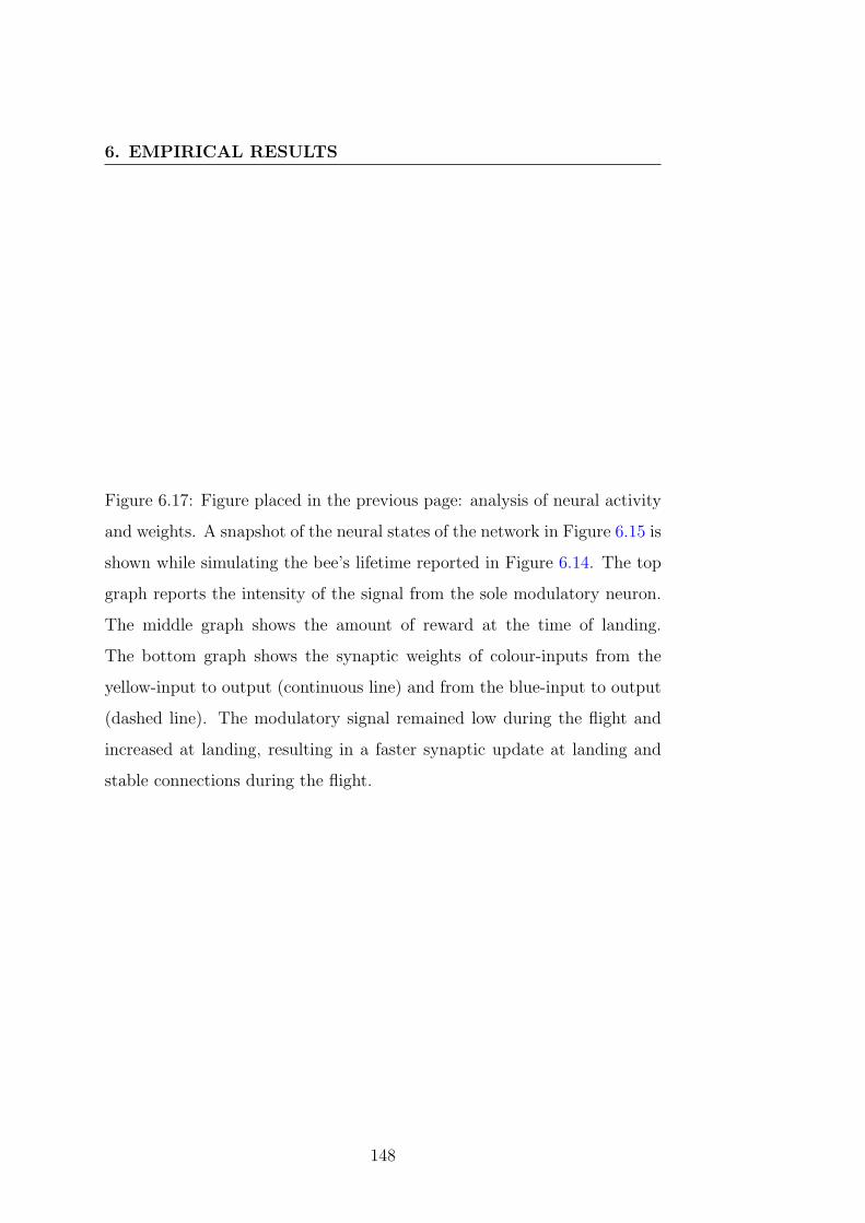
6. EMPIRICAL RESULTS
Figure 6.17: Figure placed in the previous page: analysis of neural activity
and weights. A snapshot of the neural states of the network in Figure 6.15 is
shown while simulating the bee’s lifetime reported in Figure 6.14. The top
graph reports the intensity of the signal from the sole modulatory neuron.
The middle graph shows the amount of reward at the time of landing.
The bottom graph shows the synaptic weights of colour-inputs from the
yellow-input to output (continuous line) and from the blue-input to output
(dashed line). The modulatory signal remained low during the flight and
increased at landing, resulting in a faster synaptic update at landing and
stable connections during the flight.
148

6. EMPIRICAL RESULTS
6.5 Advantages of Neuromodulation: Exper-
iments in the T-maze Problems
The studies presented so far indicated that certain types of reward-based
learning environments did not require neuromodulation. At the same time,
the experiments in Section 6.4 showed that neuromodulation could imple-
ment useful, although not essential, dynamics for reward-based learning.
Therefore, despite the insights provided so far, the role and use of neuro-
modulation remain uncertain. To provide further insight, in the experiments
presented here and summarised in (Soltoggio et al., 2008), single and dou-
ble T-mazes were used to test the emergence of modulatory dynamics, and
observe the evolving performance of controllers. The results indicated an
evolutionary advantage of networks with modulatory neurons with respect
to networks without them.
6.5.1 Evolutionary Search
The algorithm in Section 5.3 was used with the parameters listed in Table
6.3. Table 6.4 lists the parameters for the environments. Table 6.5 lists the
parameters for the neural networks. These parameters were used in this
and the following sections unless otherwise specified.
6.5.2 Experimental Results
Three types of evolutionary experiments were conducted, each characterised
by different constraints on the properties of the neural networks: 1) fixed
weight, 2) plastic, and 3) plastic with neuromodulation (also called modu-
latory networks). The fixed weight networks were implemented imposing a
value of zero on the modulatory activity, which resulted in a null update of
weights (Equation 5.4). Plastic networks had a fixed modulatory activity
149

6. EMPIRICAL RESULTS
Population (T-maze ) 300Population (double T-maze) 1000Generations (T-maze) 600Generations (double T-maze) 1000Neuron Insertion probability 0.04Neuron Duplication probability 0.02Neuron Deletion probability 0.06Mutation rate (parameter P in Eq. 5.10) 180Crossover probability 0.1Tournament size 5
Table 6.3: Parameters for the evolutionary runs for the experiments inSection 6.5.
Number of lives per fitness evaluation 4Number of trials per life (T-maze) 100Number of trials per life (double T-maze) 200Value of high reward 1.0Value of low rewards 0.2Duration of stationary conditions (in trials) 50±15Penalty for crush (summed on total fitness) -0.3Penalty for wrong homing direction(summed on total fitness)
-0.3
Noise range 1%Range of A,B,C,D (in Eq. 5.5) [-1,1]Range of η (in Eq. 5.5) [-100,100]Variable corridor length 1-3 IO steps
Table 6.4: Parameters for the T-mazes.
of 1 so that all synapses were continuously updated (Equation 5.4 becomes
∆w = 0.462 · δ). Finally, neuromodulatory plastic networks could take
advantage of the full model described in Equations 5.1-5.5.
Fifty independent runs were executed for each of the three conditions.
For each run, the individual that performed best at the last generation was
tested 100 lifetimes with different initial conditions. The average reward
collected over the 100 tests was the numerical value of the performance. The
procedure was repeated for all the 50 independent runs. The distribution
150

6. EMPIRICAL RESULTS
Maximum number of nodes 16Values for weights [-10,10]Minimum initial values for weights 0.1Neural steps per IO refresh 3
Table 6.5: Parameters for the neural networks in Section 6.5.
of performance is summarised by box plots in Figure 6.18 for the single
T-maze, and in Figure 6.19 for the double T-maze.
For the single T-maze, the theoretical and measured maximum amount
of reward that could be collected on average was 98.8, and not 100 due to
the minimum amount of exploration that the agent needed to perform at
the beginning of its lifetime and when the reward changed position. For the
double T-maze, the theoretical and measured maximum amount of reward
that could be collected was 195.2 when averaged on many experiments.
The experimental results indicated that plastic networks achieved far
better performance than the fixed weight networks. Fixed weight networks
displayed some levels of adaptive behaviour by exploiting recurrent connec-
tions, and storing state-values in the activation of neurons as in (Blynel
and Floreano, 2002; Stanley and Miikkulainen, 2003a). However, the ex-
periments here showed that such solutions were more difficult to evolve.
Among plastic networks, those that could exploit modulation displayed
a small advantage in the single T-maze. However, when memory and learn-
ing requirements increased in the double T-maze, modulated plasticity dis-
played a considerable advantage. Figure 6.19 shows that modulatory net-
works achieved nearly optimal performance in the double T-maze experi-
ment.
It is important to note that the exact performance reported in Figures
6.18 and 6.19 depend on the specific design and settings of the evolutionary
search. Higher or lower population numbers, available generations, different
151

6. EMPIRICAL RESULTS
Fix−weight Plastic Modulatory
30
40
50
60
70
80
90
100
Per
form
ance
Figure 6.18: Box plots with performances of 50 runs on the single T-maze
with homing. The boxes are delimited by the first and third quartile, the
line inside the boxes is the median value while the whiskers are the most
extreme data samples from the box not exceeding 1.5 times the interquartile
interval. Values outside this range are outliers and are marked with a cross.
Boxes with non overlapping notches have significantly different median (95%
confidence) (Matlab, 2007)
selection mechanisms and mutation rates affect the final fitness achieved in
all cases of fix-weight, plastic and modulatory networks. However, a set of
preliminary runs performed by varying the above settings confirmed that
the differential in performance between modulatory networks and plastic
or fix-weight networks was consistent, although not always the same in
magnitude.
152

6. EMPIRICAL RESULTS
Fix−weight Plastic Modulatory
20
40
60
80
100
120
140
160
180
200P
erfo
rman
ce
Figure 6.19: Box plots with performances of runs on the double T-maze
with homing.
6.5.3 Analysis and Discussion
The agents achieving optimal fitness in the tests displayed an optimal con-
trol policy of actions. This consisted in adopting an exploratory behaviour
initially – until the location of the high reward was identified – followed by
an exploitative behaviour of returning continuously to the location of the
high reward. Figure 6.21 shows an evolved behaviour, analogous to operant
conditioning in animal learning. This policy involved the exploration of the
4 maze-ends. When the high reward was discovered, the sequence of turning
actions that led there, and the correspondent homing turning actions, were
retained. That sequence was repeated as long as the reward remained in the
same location, but was abandoned when the position of the reward changed.
At this point the exploratory behaviour was resumed. The alternation of
153

6. EMPIRICAL RESULTS
ST 1
MOD 2
MOD 1
Out
Reward
Turn
Home
-9.93-1.57
2.01
-2.12
M-Einputs
Bias
-2.85-4.55 8.25
0.23
-2.58
-2.58
8.23
-8.48
Figure 6.20: Example of an evolved network that solved the double T-maze
with homing. This network has two modulatory neurons, and inner stan-
dard neuron and the output neuron (also standard). Arcs represent synaptic
connections. The inputs (Bias, Turn, Home, M-E, Reward) and standard
neurons (ST 1 and OUT) send standard excitatory/inhibitory signals to
other neurons. Modulatory neurons (MOD 1 and MOD 2) send modula-
tory signals which affects only plasticity of postsynaptic neurons, but not
their activation level. The evolved plasticity rule was A = 0, B = 0,
C = −0.38, D = 0, η = −94.6. This network has only feed-forward con-
nections, however, a number of other well performing networks displayed
recurrent connections as well.
exploration and exploitation driven by search and discovery of the reward
continued indefinitely across trials.
Although this strategy was a mandatory choice to maximise the to-
tal reward, the performance indices (Figures 6.18 and 6.19) indicate that
this behaviour could be more easily evolved when modulatory neurons were
available to evolution.
154

6. EMPIRICAL RESULTS
21
41
161
Legend:
End explored
by the agent
Location of the
high reward
Dot
Coloured area
End 0 (LL-RR)
End 1 (LR-LR)
End 2 (RL-RL)
End 3 (RR-LL)
Trials
Figure 6.21: See caption in the next page.
155

6. EMPIRICAL RESULTS
Figure 6.21: Figure in the previous page: behaviour of an agent in the
double T-maze of Figure 4.6. A test of 80 trials was performed. The four
horizontal lines track the events at each of the four maze-ends. The position
of the reward was changed every 20 trials. The coloured area indicates where
the high reward was located. The black dots show the maze-end explored by
the agent at each trial. The agent adopted an explorative behaviour when
it did not find the high reward, and settled on an exploitative behaviour
after the high reward was found.
6.5.4 Functional Role of Neuromodulation
The experimental data on performance showed a clear advantage for net-
works with modulatory neurons. Yet, the link between performance and
characteristics of the networks was not easy to find due to the large vari-
ety of topologies and plasticity rules that evolved from independent runs.
Figure 6.20 shows an example of a network that solved the double T-maze.
The neural topology, number of neurons and plasticity rule may vary con-
siderably across evolved networks that performed equally well.
Nonetheless, it was possible to check if the better performance in the
double T-maze agents evolved with neuromodulated plasticity was corre-
lated with a differential expression of modulatory and standard neurons.
The architecture and composition of the network are modified by genetic
operators that insert, duplicate and delete neurons. The average number of
the two types of neurons was measured in evolving networks for the condi-
tion where plasticity was not affected by modulation (Figure 6.22, top left
graph) and for the condition where plasticity was affected by modulatory
inputs (Figure 6.22, bottom left graph). In both conditions, the number
of modulatory neurons was higher than the number of standard neurons.
156

6. EMPIRICAL RESULTS
0 200 400 600 800 10000
100
200
Mod
ulat
ory
Effe
ct E
nabl
ed
F
itnes
s
1200 1400 1600 1800 2000
0
100
200
Mod
ulat
ory
Effe
ct D
isab
led
F
itnes
s
1
2
3
4
Num
ber
of N
euro
ns
Neuron insertion/duplication active
0
1
2
3
4
5No neuron insertion/duplication
Num
ber
of N
euro
ns
Fitness
Standard NeuronsModulatory Neurons
Figure 6.22: Fitness (continuous line) and number of inner neurons (dashed
lines for standard and dotted lines for modulatory) in networks during evo-
lution (average values of 50 independent runs).
However, the presence of modulatory neurons when those were not active
(top left graph) depended only on insertion, duplication and deletion rates,
whereas in the case when they were enabled (bottom left graph) their pres-
ence might be linked to a functional role. This fact was suggested by the
higher value of the mean fitness.
In a second phase, the evolutionary experiments were run for additional
thousand generations, but the probability of inserting and duplicating neu-
rons was set to zero, while the probability of deleting neurons was left
unchanged. In both conditions all types of neurons slightly decreased in
number. However, modulatory neurons completely disappeared in the con-
dition where they had no effect on plasticity (Figure 6.22, top right graph)
157

6. EMPIRICAL RESULTS
0 200 400 600 800 1000 1200 1400−10
0
10
20
30
40
50
60
Generations
Fitn
ess
of m
odul
ator
y ne
twor
ks m
inus
fit
ness
of p
last
ic n
etw
orks
single T−maze
double T−maze
double T−maze homing
Figure 6.23: Differential measurements of fitness. Each line represents the
difference in fitness between runs with modulatory neurons and runs with-
out (each set is represented by the median fitness from 50 independent
runs). The evolutionary advantage of modulatory neurons is described by
the tendency of values of being positive. The evolution in the single T-maze
was stopped at generation 600 as it reached stationary conditions.
while on average two modulatory neurons were observed in the condition
where modulation could affect plasticity. This represents a further indi-
cation that neuromodulation of synaptic plasticity is responsible for the
higher performance of the agents in the double T-maze and that they play
a functional role in guiding reward-based learning.
Comparing the box plots in Figures 6.18 and 6.19, it appears that mod-
ulatory neurons provided a considerable advantage in the double T-maze
158

6. EMPIRICAL RESULTS
with homing, but not so in the single T-maze. This finding led to the
hypothesis that modulatory neurons are advantageous when the problems
increase in difficulty. To verify this statement, the evolutionary progress of
three experiments with increasing complexity were compared: 1) a single
T-maze with homing, 2) a double T-maze without homing and 3) a double
T-maze with homing. In the first problem, a 2-armed bandit problem, there
are two actions to be repeated each trial: an outgoing direction and a re-
turn direction. The return direction is always the opposite of the outgoing
direction. In the second problem, a 4-armed bandit problem, two outgoing
directions (two consecutive turns) must be learnt. In the third problem, two
outgoing and two return directions must be learnt. It was therefore assumed
that the three problems were ordered by increasing difficulty9. The median
fitness values from two sets (one with modulatory neurons and one without
modulatory neurons) of 50 independent runs were compared. Figure 6.23
shows the difference between the fitness with modulatory neurons and the
fitness without modulatory neurons. A positive line indicates an advantage
with modulatory neurons, a negative line indicates a disadvantage. The dif-
ferential fitness at the beginning of evolution is negligible, meaning that the
initial random networks performed similarly whether they had or had not
modulatory neurons. However, while evolution progressed, networks that
could receive modulatory neurons by random mutations increased rapidly
their performance manifesting a significant gap with networks that could
not employ modulatory neurons. It is possible to note that the evolution-
9It is important to note that the finding that neuromodulation gives an evolutionary
advantage in increasingly complex problems derived from the experiments. The compar-
ison of fitness progress among experiments with different complexity proposed hereafter
was conceived as part of the analysis, and it cannot be considered part of the methodol-
ogy.
159

6. EMPIRICAL RESULTS
ary advantage appeared related to the problem complexity: whereas in the
single T-maze there is only a minimal difference in fitness, and a slight
disadvantage of modulatory neurons initially, the double T-maze and the
double T-maze with homing benefit considerably by the presence of mod-
ulatory neurons. Ideally, if the advantage manifests itself only in speed of
evolution, after a period in the positive area, the lines would approach null
values towards the end of evolution, implying that the advantage is evolu-
tionary only, and not computational. On the contrary, when lines stabilise
at values different from zero, two cases are possible: either the limitations
of the evolutionary algorithm did not allow for the successful evolution of
one of the two sets, or the networks of one of the two sets have a computa-
tional advantage over the others. Figure 6.23 supports the hypothesis that
modulated plasticity evolves to benefit networks in increasingly complex
problems.
A further test was conducted on the evolved modulatory networks when
the evolutionary process was completed. Networks with high fitness that
evolved modulatory neurons were tested with modulation disabled. The
test revealed that modulatory networks, once deprived of modulatory neu-
rons, were still capable of navigation by turning at the required points and
maintaining straight navigation along corridors. The low level navigation
was preserved and the number of crashes did not increase. However, most
networks seemed capable of turning only in one direction (i.e. always right,
or always left), therefore failing to perform homing behaviour. None of the
networks appeared to be capable of reward-seeking behaviour, curiously
evoking anhedonic behaviour (Berridge and Robinson, 1998). Generally,
networks that were evolved with modulation and that were downgraded to
plastic networks (by disabling modulatory neurons) performed worse than
those evolved without modulatory neurons. Hence, it can be assumed that
160

6. EMPIRICAL RESULTS
modulatory neurons are employed to design a different neural dynamics
that, according to the experiments, were easier to evolve, and on average
empowered solutions with an important advantage.
6.5.5 Conclusion
The model of neuromodulation described here applies a multiplicative effect
on synaptic plasticity at target neurons, effectively enabling, disabling or
modulating plasticity at specific locations and times in the network. The
evolution of network architectures and the comparison with networks un-
able to exploit modulatory effects showed the advantages brought in by
neuromodulation in environments characterised by distant rewards and un-
certainties. The increased complexity of the problems appeared to outline
distinctly the advantages of neuromodulated plasticity that was more evi-
dent in the most difficult problems. The random insertion of modulatory
neurons appeared not to affect significantly the search on the single T-
maze where neuromodulation was not necessary. A correspondence between
performance and architectural motifs was not observed, however it can be
assumed that the unconstrained topology search combined with different
evolved plasticity rules allowed for a large variety of well performing struc-
tures. In this respect, the search space was explicitly unconstrained in order
to assess modulatory advantages independently of specific or hand-designed
neural structures. In this condition, the phylogenetic analysis of evolving
networks supports the hypothesis that modulated plasticity is employed to
increase performance in environments where sparse learning events demand
memorisation of selected and timed signals.
161

6. EMPIRICAL RESULTS
6.6 Increasing the Decision Speed in a Con-
trol Problem with Neuromodulation
6.6.1 Summary
The experiments of the previous section were reproduced here to perform
further analysis on the networks. The analysis shows that neuromodula-
tion does not only allow for better learning, but accelerates part of the
computation in decision processes. This appears to derive from topologi-
cal features in modulatory networks displaying more direct sensory-motor
connections, whereas non-modulatory networks require longer pathways for
signal processing. This computational advantage in increased decision speed
could contribute to unveil the fundamental role of neuromodulation in neu-
ral computation.
6.6.2 Network Topologies
New tests indicated that 47 out of 50 runs with modulatory neurons and 4
out of 50 runs with standard plasticity solved the double T-maze with hom-
ing. The problem was considered solved when an agent scored on average
at least 180 of total reward collected, out of 200 available 10.
To compare network features, two fundamental points have to be con-
sidered: 1) different runs evolved considerably different topologies, number
of neurons and plasticity rules; 2) plastic networks, achieving inferior per-
formance, had a more limited functionality than modulatory networks. In
light of this, comparing modulatory networks that solved the problem with
plastic networks that failed on average was not considered significant. As a
10Because the location of the reward is hidden to the agent, until it comes across it,
the maximum fitness is 195.2 due to the exploratory trials that occur initially and when
the reward changes location.
162

6. EMPIRICAL RESULTS
result of this last observation, it was decided to consider for analysis only
the networks that achieved full functionality: in all, 47 modulatory net-
works, and 4 plastic networks. Unfortunately, the small number of plastic
networks did not allow for a sufficient statistical analysis. Consequently,
an additional 100 runs were launched, resulting in 7 new successful stan-
dard plastic networks. In conclusion, the statistical analysis was carried out
considering 11 plastic networks and 20 modulatory networks.
Even considering networks with similar performance, the evolutionary
process designed a large variety of neural topologies, number of neurons and
plasticity rules across different independent runs. However, this was true
particularly for modulatory networks: a closer inspection revealed that stan-
dard plastic networks evolved less diverse topologies, although a measure
of diversity in topology was not attempted here. An example is reported
in Figure 6.24. Modulatory networks had an average of 3.7 neurons and
17.4 connections with standard deviations of 0.9 and 9.2 respectively, re-
sulting in high diversity of networks, all of them however achieving optimal
behaviour. This finding might contribute to explain the considerable differ-
ence in successful rate of the evolutionary runs: while standard networks
achieve full functionality with only one specific architecture, modulatory
networks display a variety of topologies with optimal performance. This
suggests that the search space – when modulatory neurons are introduced –
becomes richer of multiple global optimal solutions. It is also possible that
modulatory neurons create neutral paths in the search space, allowing for
a higher evolvability (Smith et al., 2002a).
6.6.3 Decision Speed
Despite the number of neurons varied across different modulatory networks,
the input and output, imposed by the environmental settings, were the same
163

6. EMPIRICAL RESULTS
ST 1
Out
Reward TurnHome
-1.84
9.9
9.86
inputs
ST 2
-0.37
9.86
0.1
turn-to-out pathway
Bias
Figure 6.24: Example of a plastic network achieving near-optimal perfor-
mance (plasticity rule A:-0.261,B:0,C:-1,D:0,η:-31.8). All plastic networks
that were analysed had one inner neuron between the turning signal and
the output.
for all networks. On this basis, it was appropriate to compare input-output
signal propagation considering the networks as a black box.
Surprisingly, the analysis revealed that the outputs of modulatory net-
works on average appeared to react faster at turning points than the output
of plastic networks. Figure 6.25 shows the absolute values of the output
neurons (one for each network) when the network under test encountered a
turning point. The number of computational steps required by modulatory
networks to indicate a turning direction was 1.43 (average on 20 networks).
Plastic networks, on the other hand, took 2.21 steps (average on 11 net-
works) to indicate the turning preference. Moreover, Figure 6.25 shows
that whereas a substantial number of modulatory networks reacted in one
step, none of the plastic networks had such a short reaction time.
The turning action expressed by the output is a required reaction at
turning points: failure to turn resulted in the agent crashing. Therefore, it
164

6. EMPIRICAL RESULTS
0
0.33
1
Out
put
(M
odul
ator
y N
etw
orks
)
S S S0
0.33
1
Out
put
(Pla
stic
Net
wor
ks)
Figure 6.25: Absolute values of output signals at a turning point of modula-
tory and plastic networks with similar performance. Modulatory networks
(upper graph) appeared to react faster to the turning point and provided a
quicker decision. Plastic networks show a longer reaction time. The thick
vertical lines indicate the constraints at Sampling points (S): the first line
from left indicates that the output is required to be less than 0.33 (to main-
tain a straight direction in the corridor). The second line shows that the
output is required to be higher in absolute value than 0.33 (to perform a
turning action).
was assumed here that the relevant part of the computation involved in the
decision of which direction to take had to lie in the pathway between in the
turn-input signal and the output. Accordingly, the network topologies were
analysed to discover relevant features in pathways from turn-input to output
neuron. The networks resulted in having, on average, a distance of 1.1 con-
nections between input and output in the modulated case. Plastic networks
had always 2 connections between turn-input and output, i.e. there was
165

6. EMPIRICAL RESULTS
turn-to-out pathway
ST 1
MOD 2
MOD 1
Reward TurnHome
-9.93
-1.57
2.01-2.12
inputs
Bias
-2.85-4.55
8.25
0.23
-2.58
-2.58
8.23
-8.48
Out
Figure 6.26: Example of a modulatory network achieving near-optimal per-
formance (plasticity rule A:0, B:0, C: -0.38, D:0, η: 94.6). Some of these
networks, like in this case, show a direct connection between turning input
and output. None of the plastic networks showed such a feature.
never a direct connection between turn-input and output. The number of
connections through which the turn-input propagates corresponded approx-
imately to the time required to complete the computation at the turning
point and provide a direction of navigation at the output neuron. For mod-
ulated networks, a direct connection between turn-input and output was
frequently present; in plastic networks, the turn-input required to be pro-
cessed by one inner neuron. Examples of two representative networks are
shown in Figure 6.24 for a plastic network and Figure 6.26 for a modulated
network.
According to the experimental settings, the networks were given three
computational steps for each sensory-motor (input-output) update. The
output of the network was sampled each three network steps, implying that
no difference in behaviour or fitness could be detected if the output changed
in 1, 2 or 3 computational steps. so long as the output reached the required
166

6. EMPIRICAL RESULTS
level before being sampled (see Figure 6.25). Therefore plastic networks
derived no disadvantage on performance11 by having a path of two serial
connections between turn-input and output. Such configuration might have
originated from implementation aspects of the evolutionary process.
Similarly, although modulatory networks display frequently a direct turn-
input to output connection, it is not excluded that other parts of the network
required longer processing time. In fact, the inspection of modulatory net-
works showed other longer pathways departing from input signals like the
reward or home and innervating other neurons. Hence, although the anal-
ysis so far seems to indicate a faster computation for the decision process
in modulatory networks, a further test presented in the next section was
necessary.
6.6.4 Enforcing Speed
Reducing the available computational time at decision points (turning points)
was a way of compelling networks to react quickly. Accordingly, a new evo-
lutionary process was devised with identical settings as previously, but with
only one computational step available at critical points in the maze. All
the grey areas in the maze of Figure 4.6 were presented to the network for
one computational step only. The new constraint required networks to take
decision at turning points in one computational step. In this condition,
networks could achieve high performance only if capable of evolving direct
input-output paths.
The results of 50 independent evolutionary runs are illustrated in Figure
6.27, and in the box plots of Figures 6.28. The data show that plastic net-
works did not evolve to solve the learning task, implying that the constraint
on the decision speed was determinant. This result suggests that the inner
11Modulatory and plastic networks with identical performance are compared here.
167
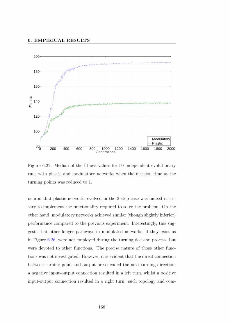
6. EMPIRICAL RESULTS
0 200 400 600 800 1000 1200 1400 1600 1800 200080
100
120
140
160
180
200
Generations
Fitn
ess
ModulatoryPlastic
Figure 6.27: Median of the fitness values for 50 independent evolutionary
runs with plastic and modulatory networks when the decision time at the
turning points was reduced to 1.
neuron that plastic networks evolved in the 3-step case was indeed neces-
sary to implement the functionality required to solve the problem. On the
other hand, modulatory networks achieved similar (though slightly inferior)
performance compared to the previous experiment. Interestingly, this sug-
gests that other longer pathways in modulated networks, if they exist as
in Figure 6.26, were not employed during the turning decision process, but
were devoted to other functions. The precise nature of those other func-
tions was not investigated. However, it is evident that the direct connection
between turning point and output pre-encoded the next turning direction:
a negative input-output connection resulted in a left turn, whilst a positive
input-output connection resulted in a right turn: such topology and com-
168

6. EMPIRICAL RESULTS
Plastic Modulatory
100
110
120
130
140
150
160
170
180
190
Per
form
ance
Figure 6.28: Box plots with performances of 50 runs with the additional
constraint of one computational step at turning points. Note that, although
these boxes were computed for the solutions at the end of the runs plotted
in Figure 6.27, median values displayed here are lower than the median
values in Figure 6.27. This is due to the fact that the values in Figure
6.27 are the medians of best fitness from the runs, whereas the median
in this figure are computed after the evolutionary by performing a test on
100 agent-lives. Note that although modulatory networks registered slightly
decreased performance, plastic networks were unable to evolve any optimal
solution.
putation were observed only in modulatory networks where a change in the
sign of the connection between turn-input and output resulted in the alter-
nation of left and right turns. Given that the plastic networks were unable
169

6. EMPIRICAL RESULTS
to achieve this, neuromodulation was responsible for a pre-computation that
resulted in the hard-wiring of the next turning direction. Subsequently, the
pre-computed information resulted in a faster decision process at turning
points.
6.6.5 Conclusion
This study considered performance and computational aspects of plastic and
modulated networks evolved in a dynamic, reward-based scenarios where
learning events (reward intake) and decision processes (turning points) de-
termined the fitness of an agent. The learning capabilities of modulatory
networks were evolved here in order to analyse computational and topo-
logical aspects of networks with and without modulatory neurons. A fun-
damental difference between plastic and modulatory networks was shown
in an increased sensory-motor propagation speed and quicker responses in
decision making for modulatory networks with respect to standard plastic
networks. At a further inspection, this property appeared to derive from
more direct sensory-motor connections in modulatory networks. The mag-
nitude and signs of those direct connections stored a value that indicated
the direction for the next turning point. This fact suggests that the decision
at turning points was pre-computed and hierarchically stored by neuromod-
ulation onto the sensory-motor direct connection. This resulted in a faster
signal processing during decision processes.
Modulated networks displayed a faster input-output response than plas-
tic networks even without strict speed constraints. However, when the speed
constraint was imposed in the second evolutionary experiment, forcing con-
trol networks to take quick turning decisions at turning points, modulatory
networks exhibited an even more considerable advantage in performance by
evolving successful solutions where plastic networks failed.
170

6. EMPIRICAL RESULTS
The evolved modulatory networks have features that depend strongly on
the environment in which the networks are evolved. This study on a single
learning problem, although complex, does not allow one to generalise the
results to other learning problems. However, the interesting computational
features displayed in this particular instance could possibly emerge in a
variety of similar or more complex learning problems. The results suggest
the possible application of the model to a variety of learning and decision
making problems.
171

6. EMPIRICAL RESULTS
6.7 A Reduced Plasticity Model: Evolving
Learning with Pure Heterosynaptic Plas-
ticity
6.7.1 Summary
Is it possible to solve learning problems with pure heterosynaptic plasticity?
If so, do networks with heterosynaptic plasticity evolve within comparable
time to networks with homosynaptic plasticity? Given the plasticity model
in this thesis, pure heterosynaptic plasticity occurs when D only is enabled
in Equation 5.5. In such case, an adaptive network can be divided in two
parts: 1) a network that performs a low level computation (similar to the
actor in actor-critic structures) and 2) a higher level network that computes
the weight updates (similar to the critic in actor-critic structures). However,
the notion of actor and critic applies to reinforcement learning or supervised
learning where the weight update is done in order to change a strategy, or
minimise an error. Here, the weight update is seen as a general mechanism
to achieve a larger set of dynamics, e.g. continuous adaptation, temporal
dynamics or oscillatory patterns. The evolution of unconstrained topolo-
gies that combine a dual structure of 1) processing signal and 2) updating
connections is not trivial, and to the best of my knowledge has not been
attempted yet. The model presented in this thesis can be easily devolved to
such attempt by clamping A,B, and C of Equation 5.5 to zero. The plastic-
ity rule in this experiment was that of Equation 5.9. Given the modulation
at the neuron-scale, all the incoming synapses of a certain neurons are up-
dated simultaneously and with the same update by incoming modulatory
signals.
172

6. EMPIRICAL RESULTS
0 200 400 600 800 1000100
110
120
130
140
150
160
170
180
190
200
Generations
Fitn
ess
Figure 6.29: Graph of the best fitness functions from the 30 independent
runs that evolved solutions with pure heterosynaptic plasticity for the dou-
ble T-maze without homing. Three runs out of 30 did not achieve opti-
mal behaviour within the limited number of generations. Twenty seven
runs evolved the correct behaviour employing only heterosynaptic non-
associative plasticity.
6.7.2 Results
Thirty independent evolutionary runs were launched with the double T-
maze. The plasticity rule of Equation 5.5 was D = 1, and A,B,C = 0. A
thousand generations were performed with a population of 1000 individuals.
Figure 6.29 shows the best fitness from the 30 runs. The graph indicates that
adaptive learning behaviour was evolved to achieve optimal performance.
Three runs out of 30 did not achieve optimal performance.
173

6. EMPIRICAL RESULTS
The inspection of the networks that solved the problem optimally re-
vealed completely different topological features, generally showing a higher
number of neurons and connections. Nevertheless, an identical evolutionary
algorithm with the same settings of Section 6.5 was able to design easily
optimal solutions.
6.7.3 Conclusion
Pure heterosynaptic plasticity can achieve remarkable levels12 of learning
and adaptation when networks are designed by artificial evolution in the
framework of the experiments in this thesis. The results suggest that the
availability of a pure heterosynaptic mechanism is not negligible and could
help achieving specific computational requirements. Modulatory neurons,
when those were the only vehicle of plasticity, appeared to be a powerful
element in the evolution of adaptation. An important conclusion is that
heterosynaptic plasticity in the absence of associative Hebbian plasticity
evolved solutions comparable in performance to those that used the com-
plete set of associative Hebbian and non-associative rules of Equation 5.5
without neuromodulation. In other words, the availability of sole heterosy-
naptic plasticity allowed for the evolution of solutions to the same tasks
that in the previous experiments was tackled with substantially different
computation. Heterosynaptic plasticity is shown here for the first time to
be a powerful and independent neural mechanism for adaptation, learning
and memory.
12Here, by remarkable, it is intended that the performances achieved by the evolved
networks with sole heterosynaptic plasticity surpass those of fixed-weight or plastic net-
works as presented in Section 6.5. Hence, although remarkable does not express an
absolute or precise measure, the term must be intended with respect to the experimental
results illustrated in this thesis.
174

6. EMPIRICAL RESULTS
6.8 Adaptation without Rewards: An Evo-
lutionary Advantage of Neuromodulation
6.8.1 Summary
All the environments introduced so far can be classified as hidden semi-
Markov processes because the location of the reward is hidden to the agent.
The location of the reward, and consequently the best course of actions,
must be discovered by the agent by means of exploratory trials, which – de-
spite being a cost – are essential to identify the correct actions and maximise
the overall reward intake.
A different class of problems was introduced here by making visible the
location of the reward, i.e. allowing the agent to ‘see’ where the high reward
was located by adding sensory information. To implement this, the agent
was given an extra set of inputs that disclosed the location of the reward
before hand. These inputs can be seen as static conditioned stimuli. Because
of that, conditioning can take place on the evolutionary scale, and lifetime
learning is not required. In these conditions, a well performing controller did
not necessitate exploratory trials because it could exploit immediately the
high rewarding maze-end. When the reward location was changed, the agent
was informed by an update of the input that disclosed the reward location.
In a way, these environments might not be considered reward-based because
the reward information is redundant. In other words, although an optimal
controller is required to perform the same output actions as in the hidden-
reward T-maze, the current set of input is sufficient to determine the optimal
future course of action without temporal learning. The reward information
becomes redundant once a correct input-output mapping has been acquired
on the evolutionary scale. On the time scale of more trials (lifetime), the
network can be seen as purely reactive. Because of this, it can be said
175

6. EMPIRICAL RESULTS
that the agent does not require learning. However, particular care must be
taken in using the last proposition, once again for the imprecise meaning of
learning in this context. When looking at a shorter time scale, for instance
inside one trial, temporal dynamics and memory (to distinguish the first
turning point from the second) are required. The experiments in this section
were performed to assess the evolutionary advantages of modulated neurons
in the condition described above.
6.8.2 Results
In a double T-maze, an agent was given four extra bit-inputs that disclosed
the location of the reward. Each extra input represented one maze-end,
and the bit-input associated with the high-rewarding maze-end was high,
whereas the other inputs were low. All other parameters and settings were
identical to those specified in Section 6.5. Fifty independent evolutionary
runs were launched to evolve networks with and without modulatory neu-
rons. The fitness progress of all the 50 runs is shown in Figures 6.30 and
6.31. It is possible to note the faster evolution of networks with modulatory
neurons. In this problem where rewards are not hidden, an agent can collect
all the 200 available rewards because there is no need for exploration.
6.8.3 Conclusion
A considerable advantage was observed in evolutionary runs that could in-
sert modulatory neurons. This fact indicates that modulatory neurons help
achieving higher levels of adaptation even when environments are not char-
acterised by hidden, uncertain rewards. Such a finding implies that the role
of neuromodulated plasticity is not exclusively related to the processing and
interpretation of reward signals or prediction error signals. On the contrary,
neuromodulated plasticity appears to play a fundamental role in the basic
176

6. EMPIRICAL RESULTS
0 200 400 600 800 100080
100
120
140
160
180
200
Generations
Fitn
ess
Figure 6.30: Fitness progress during evolution in a double T-maze with
non-hidden rewards for the runs with modulatory neurons.
0 200 400 600 800 100080
100
120
140
160
180
200
Generations
Fitn
ess
Figure 6.31: Fitness progress during evolution in a double T-maze with
non-hidden rewards for the runs without modulatory neurons.
177

6. EMPIRICAL RESULTS
input-output mapping processes, enabling the network to achieve complex
and varying temporal dynamics. Therefore, such dynamics do not necessary
represent a learning process, but more generally an adaptation process. In
a broad sense, this result invites one to consider neuromodulated plasticity
as a computational tool affecting very basic and general neural functions
such as adaptive input-output mapping and temporal dynamics.
178

Chapter 7
Conclusion
7.1 Summary of Main Findings
This thesis proposed the evolution of neural networks of arbitrary size and
topology where the neurons were instances of two different types, standard
and modulatory. Such a distinction was inspired partly by the variety of
neuron types with modulatory dynamics in biology, and partly by the neces-
sity of addressing limitations in learning and adaptation of current neural
models. The intent was the investigation of the use and advantages of
neuromodulated plasticity where sparse learning events demand localised
updates in a neural network, and the memorisation of selected and timed
signals. The model of a modulatory neuron, and the effect of such a neuron
type on the network, were introduced resulting in the implementation of a
set of homo- and heterosynaptic plasticity mechanisms. The model of mod-
ulatory neurons applies a multiplicative effect on the synaptic plasticity at
target neurons, enabling, disabling or modulating plasticity at specific lo-
cations and times in a network. The evolution of arbitrary topologies with
two types of neurons was conceived to produce networks with rich dynamics
that enabled the enhancement of learning and memory function.
Dynamic, reward-based scenarios were introduced and described here
179

7. CONCLUSION
with the two-fold purpose of creating learning environments on which to
run evolution, and to assess and compare adaptation skills and memory
function of evolved neural controllers.
Evolutionary processes sought the emergence of adaptive behaviour in
uncertain environments by using a performance-based selection mechanism
applied during the automatic design procedure for neural controllers. The
evolutionary processes were devised to search arbitrary topologies of plastic
and modulated networks without topological constraints. This feature was
important to assess the effect of modulatory dynamics with a minimal set
of assumptions on the networks.
Thus, the experimental work in this thesis was based on three mainstays.
First and most important, the introduction of a new class of modulatory
neurons; second, the search of neural topologies by means of simulated
evolution; and third, the testing in closed-loop of learning and memory
skills in dynamic, reward-based scenarios.
The combination of these three mainstays unfolded in a series of ex-
perimental findings whose main messages confirmed the two general hy-
potheses of Section 5.4. (1) The introduction of modulatory neurons and
modulated plasticity in evolving neural networks produced an evolutionary
advantage by enhancing learning and adaptation. That evolutionary ad-
vantage emerged more strongly as the problem complexity was increased,
suggesting the fundamental role of neuromodulated plasticity in favouring
the evolution of learning and adaptation in complex problems. (2) The
introduction of modulatory neurons brought forth the synthesis of differ-
ent topological structures. In turn, such structures were observed to lead
to a computational advantage by implementing feed-forward anticipatory
control structures.
Besides the assessment of the main hypotheses, the set of experiments
180

7. CONCLUSION
presented in this thesis led to a series of important contributions to knowl-
edge in the field of ANNs, as explained in the following sub-section.
7.1.1 Contribution to Knowledge
The evolution of topologies for ANNs had been carried out so far without
enlarging the search space to unconstrained network topologies of a variable
number of nodes and node-types. Nevertheless, advances in neuroscience
indicate that the GABA-gated and NMDA-gated (inhibitory/excitatory)
neural transmission accounts only for a part of neural computation. It has
been clear now for many decades that modulatory chemicals and systems
are fundamental aspects of neural computation, with important contribu-
tions in memory function, adaptation and behavioural control. Despite
the numerous models of modulated plasticity, this thesis proposed for the
first time the evolution of artificial unconstrained network topologies with
two types of neurons in order to design and target neuromodulation. The
introduction of modulatory neurons in the evolutionary process led to a re-
markable improvement in the speed of evolution in the double T-maze test
problems.
The autonomous design of control networks with evolutionary algorithms
progressed by selecting and preserving networks with modulatory neurons
when those contributed to the improved performance. Thanks to this fea-
ture, it was not only possible to observe the phenotypical expression of
modulatory neurons when those brought about a fitness improvement, but
it was possible also to observe the absence of modulatory neurons in net-
works that did not benefit from modulated plasticity in certain problems.
This last observation led to the finding that neural networks for the solution
of basic reward-based learning problems do not require modulated plastic-
ity, questioning the validity of testing neuromodulation on such problems
181

7. CONCLUSION
as in (Montague et al., 1995; Niv et al., 2002). The experimental findings
in Sections 6.2 and 6.3 indicated that basic n-armed bandit problems, the
foraging bee problem and the single T-maze problems in uncertain environ-
ments can be solved optimally without neuromodulated plasticity.
Neuromodulated plasticity was devised here as a local, cellular mech-
anism for plasticity. The evolutionary search adopted in this thesis led
to the synthesis of emergent system level dynamics. In Section 6.5, the
performance of networks were compared: the sets that could use modula-
tory neurons and the sets that could not use them. It was possible to link
the availability of modulatory neurons to the faster evolution and superior
performance in adaptivity and memory tasks. For the first time, neuromod-
ulated dynamics were observed to emerge autonomously where the problem
required them, indicating the fundamental role of neuromodulated plastic-
ity in the evolution of learning. Moreover, the methodology proposed here
indicate that it is possible to assess experimentally which problems requires
plasticity mechanisms such as neuromodulation. The capability of perform-
ing implicitly feature-selection, i.e. preserving or leading to extinction of
modulatory neurons, proved to be a discerning tool to establish experimen-
tally which conditions require neuromodulation.
The availability of modulatory neurons resulted in the evolution of sub-
stantially different neural dynamics that in Section 6.6 were observed not
only to evolve to better adaptation levels, but also to exhibit advantageous
computational features. In the double T-maze with homing, modulatory
neurons allowed for the synthesis of a direct input-output connection, re-
sulting in a fast decision process that was not observed in plastic networks.
This computational advantage, although plausible given the intrinsic hier-
archical nature of neuromodulated plasticity, was observed to emerge au-
tonomously for the first time in the experiments of this thesis. This fact
182

7. CONCLUSION
suggests the suitability of heterosynaptic plasticity in the set of problems
that require hierarchical computing and the presence of low level short-cuts
in neural wiring.
The concept of reward-based learning in this thesis mainly referred to
the online learning skills of agents capable of exploring and exploiting an
uncertain environment and changing strategies according to changing re-
ward contingencies. In the experiment in Section 6.8, the introduction
of static conditioned stimuli was done to assess the evolutionary advan-
tages of modulatory neurons in environments where online learning was
not required, but a dynamic adaptive behaviour was still essential. This
experiment was performed to ascertain whether neuromodulated plasticity
addressed computational aspects required only in reward-based learning.
Modulated plasticity was observed to give a remarkable advantage even in
this problem without reward-based learning. The finding indicated for the
first time that modulatory neurons permeate the network with a powerful
mechanism that benefits the evolution of a rich temporal neural dynamics.
This in turn boosts the evolution of reward-based learning in uncertain en-
vironments, but possibly brings about advantages in a considerably larger
set of problems.
Finally, this thesis proposed and experimented in Section 6.7 the evolu-
tion of unconstrained topologies forming a two-layer interconnected network
of low level signal processing units (standard neurons) and hierarchical units
(modulatory neurons) for pure heterosynaptic weight update. In this case,
one sub-network processed signals, and a second sub-network was in charge
of synaptic updates. This combined network implemented a computational
paradigm that evolved remarkable levels of adaptation without homosynap-
tic or correlation-based plasticity mechanisms. This result suggested for
the first time that a fundamental basis of learning in networks might rely
183

7. CONCLUSION
only partially on correlation-based Hebbian mechanisms, and heterosynap-
tic plasticity alone could cover an essential role in the synthesis of adaptive
learning behaviour.
7.2 Future Work
The results of this study originated from the combination of the three main-
stays mentioned above. A variety of alternative studies can be thought by
changing models and settings in each of the three mainstays: neural and
modulatory model (point 1), evolutionary search procedure (point 2) and
uncertain reward-based scenarios (point 3). At the level of the model (point
1), different choices can be made on the modulatory dynamics, introducing
different kinds of modulation (e.g. modulated synaptic efficacy or output
function instead of plasticity), different neural models (e.g. spiking neu-
rons) or plasticity (e.g. BCM rule, STDP, etc.). The type of neural model
depends on the precise questions to be addressed. A related topic to the
neural models is the type of sensory-motor setting to be given, which might
considerably alter the function and evolution of neural controllers. Different
evolutionary processes and encoding methods (point 2) can be considered.
Here too, a large variety of options can be taken, for example adopting
advanced algorithms for topology search (e.g. (Gauci and Stanley, 2007)),
or developmental algorithms to grow larger adaptive networks. Finally, the
application domain (point 3) can be modified by suggesting more complex
dynamic scenarios. These can be devised with longer sequences of decisions
and actions, wider spectrum of sensory information or robotic applications.
Other future directions focus on the analysis of networks and the neural
dynamics. For example, questions that can be addressed are a) what neu-
ral dynamics lead to learning behaviour, or b) are there fixed modulatory
184
7. CONCLUSION
structures that allow certain types of learning?
The following describes in more detail four of the above research direc-
tions.
7.2.1 Modulation of Neuron Outputand Multi-neuron Type Networks
Equation 5.4 uses signals from modulatory neurons to change the rate of
plasticity on weights. For this reason, the kind of modulation described in
this thesis can be named neuromodulated plasticity. However, neuromodu-
lation can be applied as a gating signal to other processes as described in
Section 2.2.3.3. Consider a class of neurons whose outputs gate the transfer
function of neurons. Let gain be a modulatory activation driven by neurons
belonging to the class G. Then
gaini =∑j∈G
(wji · oj
)+ gainb
i , (7.1)
where i is any postsynaptic neuron, gainbi is a bias value of gain for the
neuron i, and j is a presynaptic neuron belonging to the class G. Applying
a gating operation on the output transfer function of all neurons, Equation
5.3 becomes
oi(ai) = tanh(gaini · ai) . (7.2)
A gating operation on the output function could be beneficial in those sit-
uations where sensory information or internal signals need amplification or
suppression. Modulatory dynamics of this kind in biological networks was
suggested to increase sensory flexibility (Birmingham, 2001).
The gating operation performed by neurons of the class G applies to all
neurons in the networks, i.e. standard neurons, but also modulatory neurons
(if present), and gain neurons as well. An evolutionary algorithm can be set
185

7. CONCLUSION
to build networks with three types of neurons. It is possible to hypothesise
that, similarly to modulatory neurons, gating neurons will be selected when
they bring about an advantage in performance. To test control networks
with gain neurons, either alone or in combination with modulatory neurons,
is it possible to specify a control tasks where gain neurons could be advanta-
geous, and test the hypothesis by running evolution with and without gain
neurons.
7.2.2 Neuromodulation with Continuous Time or Spik-ing Neural Models
Modulated plasticity (Equation 5.4) can be applied to any neuron model,
including continuous time or spiking neural models. A research question is
whether the hypotheses that were validated in this thesis on a rate-based
model would hold with continuous time or spiking neural models.
To investigate such a possibility, the neural and plasticity models should
be modified. In the case of continuous time neurons, it is possible to in-
troduce time constants for each neuron. Equations 5.1 and 5.2 should be
modified to include the time dynamics,
ai(t+ ∆t) = ai(t) +∆t
τ stdi
[ ∑j∈Std
(wji · oj(t)
)− ai(t)
], (7.3)
and
mi(t+ ∆t) = mi(t) +∆t
τmodi
[ ∑j∈Mod
(wji · oj(t)
)−mi(t)
], (7.4)
where the time constants for the standard activation ai(t) and for the mod-
ulatory activation mi(t), respectively τ stdi and τmod
i could be different.
For testing spiking neurons, more substantial changes are required. A
spiking neuron model should be used for both standard and modulatory
neurons. A plasticity rule, for example STDP, should be chosen to perform
186

7. CONCLUSION
weight update. Finally, the weight update should be gated by the incoming
modulatory signals.
7.2.3 Neuromodulation for Robotic Applications
The problems presented in Chapter 4 were characterised by discrete dy-
namics and limited inputs and outputs. The reasons for such configuration
were explained Section 4.4.1, and can be summarised by the need of a pre-
cise definition of problem, its temporal dynamics and memory requirement.
Nevertheless, it is possible to extend the use of evolved modulatory net-
works to more complex scenarios with larger input and output sets as in
robotics. The application of neural control networks to real robots has been
considered recently as an important validation to assess the capability of a
neural model, especially in the field of evolutionary robotics. Tow robotic
mobile platforms used in the field of evolutionary robotics are the Khepera
wheeled robot and the more recent E-puck, see Figure 7.1. Those robots of
small dimension can be used to test navigation and reward based learning in
environments that represents a real implementation of the single and double
T-maze. Experiments in this direction would cast light on the scalability of
modulatory networks on larger controllers and the consistency with which
modulatory dynamics emerge from evolution to solve a range of robotic
problems.
7.2.4 Neural Dynamics and Structures for Learning
The work in this thesis showed the advantages of modulatory neurons in
certain learning and memory problems, but the precise topologies and neu-
ral dynamics where not analysed sufficiently to understand what are the
elementary mechanisms that implemented the higher learning skills. Nev-
ertheless, some analysis was performed in order to unveil the features of
187

7. CONCLUSION
Figure 7.1: A Khepera robot (left) and an E-puck robot (right) developed
at EPFL, CH.
neural dynamics. Tracking the modulatory activities of some of the evolved
networks, it was possible to identify similar neural dynamics across different
networks solving different problems. Figure 7.2 shows the temporal dynam-
ics of the reward input, turn-input and one modulatory neuron during the
execution of a network in a double T-maze without homing. It is possi-
ble to observe that the modulatory activity was normally null (implying
no plasticity) and became high when the agent encountered the turning
points (points indicated with a and b in the graph). At the collection of
the reward, if that was high, no variation of the modulatory activity was
registered (point c in the graph). On the other hand, if a low reward was
collected, a negative value of modulatory activity was registered (point d).
In another example from a network solving the double T-maze with homing,
the activity plot in Figure 7.3 was observed. The topological structure of
this network was different from the previous one which solved the double
T-maze without homing. The double T-maze with homing presented four
turning points between rewards, rather than two turning points between re-
wards as in the double T-maze without homing. Nevertheless, the activity
of MOD 2 in Figure 7.3 is similar to the activity of the modulatory neuron
188

7. CONCLUSION
0
0.51
Reward
0
0.51
Turning points
2040
6080
100
120
140
160
−101
Tim
e st
eps
Modulatoryactivity
(a) (
b)(c
)(d
)
Figure 7.2: Neural activity of a network while performing in the doubleT-maze.
189

7. CONCLUSION
0 50 100 150 200 250 3000
0.5
1
Rew
ard
0 50 100 150 200 250 3000
0.5
1
Tur
ning
P
oint
s
0 50 100 150 200 250 300−2
−1
0
1
2
Out
put
Neu
ron
0 50 100 150 200 250 300−2
−1
0
1
2
MO
D 1
0 50 100 150 200 250 300−1
−0.5
0
0.5
1
MO
D 2
Figure 7.3: Neural activity of a network, such as that shown in Figure 6.20,
while performing in the double T-maze with homing.
of the different network and problem of Figure 7.2 (it differs only in the
sign). In both cases, the modulatory activity encoded a surprise signal that
was activated by turning points, remained null when a high reward was
obtained, and assumed opposite values to those at the turn points when a
low reward was obtained.
From these preliminary observations, it is reasonable to hypothesise that
a common high level mechanism was autonomously discovered by evolution
to solve those two different problems. The simulated evolution appeared
to have generated in two different instances a surprise signal that presents
190

7. CONCLUSION
analogies with system level prediction and error signals of dopaminergic
neurons (Schultz, 1998). Interesting questions are: what problems elicit the
autonomous emergence of surprise or prediction error signals? What neural
structures generate first and use later these signals to achieve general skills
of adaptation and learning (Schultz, 2008; Worgotter, 2008)?
191

Glossary
5-HT: 5-hydroxytryptamine, or Serotonin, a neurotransmitter of the
group of monoamines
ACh: Acetylcholine: is a neurotransmitter of the group of amines
AE: Artificial Embryogeny
Amine: An organic compound that functions as a neurotransmitter
in neural substrates. Among amine neurotransmitters are DA and
ACh
ANNs: Artificial Neural Networks
Behavioural Neuroscience: The study of behaviour as an observ-
able and emergent feature of complex neural dynamics
Cellular Neuroscience: The study of neurons and their character-
istics, variety and computational role
Classical Conditioning: ‘A form of associative learning in which
a subject learns the relationship between two stimuli’ (Bailey et al.,
2000)
Cognitive Neuroscience: the study of neural mechanisms that re-
sult in self-awareness, rational thinking, imagination, language, etc.
CPG: Central Pattern Generator
192

7. CONCLUSION
CREB: cAMP Response Element Binding proteins are transcription
factors that bind to the DNA and mediate the transcription of certain
genes.
CTRNNs: Continuous Time Recurrent Neural Networks
DA: Dopamine is an amine that acts as a neurotransmitter
EAs: Evolutionary Algorithms, including GAs, GP, ES, EP
Epigenesis (theory of): ‘the theory that the germ is brought into
existence (by successive accretions), and not merely developed, in the
process of reproduction’ (OED, 1989)
ES: Evolution Strategy
Fitness function: A measure of quality or performance of an indi-
vidual or a solution used in Evolutionary Algorithms
GABA: Gamma-aminobutryric acid, an amino acid synthesised from
glutamate, is the major inhibitory neurotransmitter in the central
nervous system (Bear et al., 2005)
GAs: Genetic Algorithms
GP: Genetic Programming
Habituation: ‘A decrease in the behavioural response to a repeated,
benign stimulus’ (Bailey et al., 2000).
Locus coeruleus: ‘Nucleus of the brain stem. The main supplier of
noradrenaline to the brain’ (Bailey et al., 2000)
LTD: Long-term depression, a long-lasting decrease in the effective-
ness of synaptic transmission that follows certain types of conditioning
stimulation
193

7. CONCLUSION
LTP: Long-term potentiation, long-lasting enhancement of the effec-
tiveness of synaptic transmission that follows certain types of condi-
tioning stimulation
Molecular Neuroscience: the study of elementary molecules that
are found in nervous systems
Neuroethology: The study of animal behaviour in relation to the
nervous systems and the underlying neural mechanisms
NE: Norepinephrine, or Noradrenaline, is a neurotransmitter of the
group of catecholamine
NMDA: N -methyl-D-aspartate is a neurotransmitter generally asso-
ciated with excitatory synapses (Gerstner and Kistler, 2002)
Ontogenesis: ‘The development of the individual organism from the
earliest embryonic stage to maturity. Also: the development of a par-
ticular (anatomical, behavioural, etc.) feature of an organism’ (OED,
1989)
Operant Conditioning: Learning to obtain reward or to avoid pun-
ishment (Britannica, 2007a)
Phylogeny: refers to ‘the history of the evolution of a species or
group’ (Britannica, 2007b).
POE model: Phylogenetic, Ontogenetic and Epigenetic model
Sensitisation: ‘The strengthening of the response to a wide variety
of neural stimuli following an intense or noxious stimuli’ (Bailey et al.,
2000).
SNNs: Spiking Neural Networks
Synapse: ‘The region of contact where a neuron transfers information
to another cell’ (Bear et al., 2005)
194

7. CONCLUSION
Synaptic Plasticity: ‘A change in the functional properties of a
synapse as a result of use’ (Bailey et al., 2000)
System Neuroscience: The study of neural dynamics that origi-
nates from the complex circuitry of connected neurons
Ventral Tegmental Area (VTA): ‘Nucleus of the midbrain. The
main supplier of dopamine to the cortex’ (Bailey et al., 2000)
195

References
Oxford English Dictionary. Oxford : Oxford University Press, 1989. 36,
193, 194
L. F. Abbott. Modulation of Function and Gated Learning in a Network
Memory. Proceedings of the National Academy of Science of the United
States of America, 87(23):9241–9245, 1990. 45, 47, 94
L. F. Abbott and S. B. Nelson. Synaptic plasticity: taming the beast.
Nature Neuroscience, 3:1178–1183, 2000. 21
L. F. Abbott and W. G. Regehr. Synaptic computation. Nature, 431:796–
803, 2004. 17, 21
W. C. Abraham and M. F. Bear. Metaplasticity: the plasticity of synaptic
plasticity. Trends in Neuroscience, 19:126–130, 1996. 42
W. H. Alexander and O. Sporns. An Embodied Model of Learning, Plas-
ticity, and Reward. Adaptive Behavior, 10:143, 2002. 65
G. W. Arbuthnott, C. A. Ingham, and J. Wickens. Dopamine and synaptic
plasticity in the neostriatum. Journal of Anatomy, 196:587–596, 2000. 19
L. Bacciottini, M. Passani, P. Mannaioni, and P. Blandina. Interactions
between histaminergic and cholinergic systems in learning and memory.
Behavioural Brain Research, 124(2):183–194, 2001. 21, 44
196

REFERENCES
T. Back and H.-P. Schwefel. An overview of evolutionary algorithms for pa-
rameter optimization. Evolutinary Computation, 1(1):1–23, Spring 1993.
50, 52
T. Back, D. B. Fogel, and Z. Michalevicz, editors. Handbook of Evolutionary
Computation. Oxford University Press, Oxford, 1997. 63, 98, 115, 138
C. H. Bailey, M. Giustetto, Y.-Y. Huang, R. D. Hawkins, and E. R. Kandel.
Is heterosynaptic modulation essential for stabilizing hebbian plasticity
and memory? Nature Reviews Neuroscience, 1(1):11–20, October 2000.
4, 24, 26, 38, 87, 192, 193, 194, 195
A. B. Barron, R. Maleszka, R. K. Vander Meer, and G. E. Robinson. Oc-
topamine modulates honey bee dance behavior. PNAS, 104(5):1703–1707,
2007. 22
D. A. Baxter, C. C. Canavier, J. W. Clark, and J. H. Byrne. Computational
Model of the Serotonergic Modulation of Sensory Neurons in Aplysia.
Journal of Neurophysiology, 82:1914–2935, 1999. 42
M. F. Bear, B. W. Connors, and M. A. Paradiso. Neuroscience: Exploring
the Brain. Baltimore, MD.; London : Williams & Wilkins, 2005. 14, 15,
17, 19, 20, 87, 91, 193, 194
R. D. Beer and J. C. Gallagher. Evolving dynamical neural networks for
adaptive behavior. Adapt. Behav., 1(1):91–122, 1992. ISSN 1059-7123.
30, 64
S. Bengio, Y. Bengio, J. Cloutier, and J. Gecsei. On the optimization of
a synaptic learning rule. In Preprints Conf. Optimality in Artificial and
Biological Neural Networks, Univ. of Texas, Dallas, Feb 6-8, 1992, 1992.
45
R. J. Beninger. The Role of Dopamine in Locomotor Activity and Learning.
Brain Research Reviews, 6:173–196, 1983. 20
197

REFERENCES
K. C. Berridge. The debate over dopamine’s role in reward the case for
incentive salience. Psychopharmacology, 191:391–431, 2007. 21
K. C. Berridge and T. E. Robinson. What is the role of dopamine in reward:
hedonic impact, reward learing, or incentive salience? Brain Research
Reviews, 28:309–369, 1998. 21, 160
L. E. Bienenstock, L. N. Cooper, and P. W. Munro. Theory for the develop-
ment of neuron selectivity: orientation specificity and binocular interac-
tion in visual cortex. The Journal of Neuroscience, 2(1):32–48, January
1982. 38, 93
J. T. Birmingham. Increasing Sensor Flexibility Through Neuromodulation.
Biological Bulletin, 200:206–210, April 2001. 43, 185
J. T. Birmingham and D. L. Tauck. Neuromodulation in invertebrate sen-
sory systems: from biophysics to behavior. The Journal of Experimental
Biology, 20:3541–3546, 2003. 22, 23
R. H. Bishop and R. C. Dorf. Modern Control Systems. Upper Saddle River.
N.J.: Prentice Hall, ninth edition, 2001. 53, 64
J. Blynel and D. Floreano. Levels of dynamics and adaptive behavior in
evolutionary neural controllers. In Proceedings of the seventh interna-
tional conference on simulation of adaptive behavior on From animals to
animats, pages 272–281. MIT Press Cambridge, MA, USA, 2002. 151
J. Blynel and D. Floreano. Exploring the T-Maze: Evolving Learning-
Like Robot Behaviors Using CTRNNs. In EvoWorkshops, pages 593–604,
2003. 30, 31, 39
R. Bogaz. Optimal decision-making theories: linking neurobiology with
behaviour. Trends in Cognitive Sciences, 11:118–125, 2006. 72
198

REFERENCES
C. Bowers. Simulating Evolution with a Computational Model of Embryo-
geny. PhD thesis, School of Computer Science, University of Birmingham,
2006. 59
V. Braitenberg. Vehicles: Experiments in Synthetic Psychology. The MIT
Press, 1984. 45
B. Brembs, F. D. Lorenzetti, F. D. Reyes, D. A. Baxter, and J. H. Byrne.
Operant Reward Learning in Aplysia: Neuronal Correlates and Mecha-
nisms. Science, 296(5573):1706–1709, 2002. 22
Britannica. Animal learning. Encyclopedia Britannica 2007 Ultimate Ref-
erence Suite, 2007a. 37, 79, 194
Britannica. Phylogeny. Encyclopedia Britannica 2007 Ultimate Reference
Suite, 2007b. 194
R. A. Brooks. A Robust Layered Control System For A Mobile Robot.
IEEE Jornal of Robotics and automation, RA-2(1):14–23, 1986. 34
J. W. Brown, D. Bullock, and S. Grossberg. How the Basal Ganglia Use
Parrallel Excitatory and Inhibitory Lerning Pathways to Selectively Re-
spond to Unexpected Rewarding Cues. The Journal of Neuroscience, 19
(23):10502–10511, 1999. 21
G. Bugmann. Biologically palusible neural computation. BioSystems, 40:
11–19, 1997. 27
J. A. Bullinaria. Understanding the Emergence of Modularity in Neural
Systems. Cognitive Science, 31:673–695, 2007. 34
B. D. Burrell and C. L. Sahley. Learning in simple systems. Current Opinion
in Neurobiology, 11:757–764, 2001. 22, 23
T. J. Carew, E. T. Walters, and E. R. Kandel. Classical conditioning in
a simple withdrawal reflex in aplysia californica. The Journal of Neuro-
science, 1(12):1426–1437, December 1981. 22, 42
199

REFERENCES
D. Centonze, B. Picconi, P. Gubellini, G. Bernardi, and P. Calabresi.
Dopaminergic control of synaptic plasticity in the dorsal striatum. Euro-
pean Journal of Neuroscience, 13(6):1071, 1077 2001. 20
J. S. Chahl, M. V. Srinivasan, and S. W. Zhang. Landing strategies in
honeybees, and possible applications to autonomous airborne vehicles.
The International Journal of Robotics Research, 23(2):101–110, February
2004. 32
C. Christodoulou, G. Bugmann, and T. G. Clarkson. A spiking neuron
model: applications and learning. Neural Networks, 15:891–908, 2002. 32
G. A. Clark and E. R. Kandel. Branch-specific heterosynaptic facilitation
in aplysia siphon sensory cells. PNAS, 81(8):2577–2581, 1984. 22, 91
J. D. Cohen, T. S. Braver, and J. W. Brown. Computational perspectives on
dopamine function in prefrontal cortex. Current Opinion in Neurobiology,
12:223–229, 2002. 88
M. X. Cohen. Neurocomputational mechanisms of reinforcement-guided
learning in humans: A review. Cognitive, Affective and Behavioral Neu-
roscience, 8(2):113–125, 2008. 44
S. J. Cooper. Donald O. Hebb’s synapse and learning rule: a history and
commentary. Neuroscience and Biobehavioral Reviews, 28(8):851–874,
January 2005. 22, 37
H. H. Dale. Pharmacology and nerve-endings. Proc. R. Soc. Med., 28:
319–332, 1935. 17, 87
C. Darwin. On the origin of species by means of natural selection, or The
preservation of favoured races in the struggle for life. Murray, London,
1859. 48
200
REFERENCES
N. D. Daw. Reinforcement learning models of the dopamine system and
their behavioral implications. PhD thesis, School of Computer Science,
Carnegie Mellon University, 2003. 19, 20
N. D. Daw and D. S. Touretzky. Long-Term Reward Prediction in TD
Models of the Dopamine System. Neural Computation, 14:2567–2583,
2002. 20
N. D. Daw, J. P. O’Doherty, P. Dayan, B. Seymour, and R. J. Dolan.
Cortical substrates for exploratory decisions in humans. Nature, 441(15):
876–879, June 2006. 44
P. Dayan and L. F. Abbott. Theoretical Neuroscience. MIT Press Cam-
bridge, MA, USA, 2001. 19, 27, 37, 38, 93
P. Dayan and B. W. Balleine. Reward, Motivation, and Reinforcement
Learning. Neuron, 36(2):285–298, October 2002. 19, 43
P. Dayan and A. J. Yu. Phasic norepinephrine: A neural interrupt signal
for unexpected events. Network: Computation in Neural Systems, 17(4):
335–350, 2006. 21
M. W. Decker and J. L. McGaugh. The role of interaction between the
cholinergic system and other neuromodulatory systems in learning and
memory. Synapse, 7:151–168, 1991. 21, 44
D. Deodhar and I. Kupfermann. Studies on Neuromodulation on Oscillatory
Systems in Aplysia, by Means of Genetic Algorithms. Adaptive Behavior,
8(3-4):267–296, 2000. 42
A. Destexhe and E. Marder. Plasticity in single neuron and circuit compu-
tations. Nature, 431:789–795, 2004. 44
J. S. Dittman and W. G. Regehr. Mechanism and kinetics of heterosynaptic
depression at a cerebellar synapse. The Journal of Neuroscience, 17(23):
9048–9059, 1997. 19
201

REFERENCES
K. Doya. Metalearning and neuromodulation. Neural Networks, 15(4-6):
495–506, 2002. 44
J.-C. Dreher and Y. Burnod. An integrative theory of the phasic and tonic
modes of dopamine modulation in the prefrontal cortex. Neural Networks,
15:583–602, 2002. 43
J. Dubnau, A.-S. Chiang, and T. Tim. Neural Substrates of Memory: From
Synapse to System. Journal of Neurobiology, 54:238–253, 2002. 44
P. Durr, C. Mattiussi, and D. Floreano. Neuroevolution with Analog Ge-
netic Encoding. In PPSN 2006, volume 9, pages 671–680, 2006. URL
http://ppsn2006.raunvis.hi.is/. 60
P. Durr, C. Mattiussi, A. Soltoggio, and D. Floreano. Evolvability of Neu-
romodulated Learning for Robots. In The 2008 ECSIS Symposium on
Learning and Adaptive Behavior in Robotic Systems, 2008. 92
J. L. Elman. Finding Structure in Time. Cognitive Science, 14:179–211,
1990. 34, 64
J. Eriksson, O. Torres, A. Mitchell, G. Tucker, K. Lindsay, D. M. Halliday,
J. Rosenberg, J. M. Moreno, and A. E. P. Villa. Spiking neural networks
for reconfigurable poetic tissue. In ICES, pages 165–173, 2003. 32, 58
M. A. Farries and A. L. Fairhall. Reinforcement Learning With Modulated
Spike Timing-Dependent Synaptic Plasticity. Journal of Neurophysiology,
98:3648–3665, 2007. 46
D. Federici. Evolving Developing Spiking Neural Networks. In Proceedings
of the IEEE Congress on Evolutionary Computation, CEC 2005, 2005a.
27, 32, 39, 58
D. Federici. Multi-level grounding and self-organization of behaviour through
evolution, development, learning and culture. PhD thesis, NTNU - Nor-
wegian University of Science and Technology, 2005b. 58
202

REFERENCES
J.-M. Fellous and C. Linster. Computational models of neuromodulation.
Neural Computation, 10:771–805, 1998. 40, 41
J.-M. Fellous and R. E. Suri. The Handbook of Brain Theory and Neural
Networks, chapter The Roles of Dopamine. The MIT Press, Cambridge,
MA, 2002. 43
D. Floreano and C. Mattiussi. Evolution of spinking neural controllers
for autonomous vision-based robots. In T. Gomi, editor, Evolution-
ary Robotics: From Intelligent Robotics to Artifical Life, volume 2217
of LNCS, pages 38–61. Springer, October 2001. 32
D. Floreano and F. Mondada. Automatic creation of an autonomous agent:
genetic evolution of a neural-network driven robot. In Proceedings of the
third international conference on Simulation of adaptive behavior : from
animals to animats 3, pages 421–430. MIT Press, Cambridge, MA, USA,
1994. 53
D. Floreano and F. Mondada. Evolution of homing navigation in a real
mobile robot. IEEE Transactions on Systems, Man, and Cybernetics–
Part B, 26(3):396–407, 1996. 34
D. Floreano and J. Urzelai. Neural morphogenesis, synaptic plasticity, and
evolution. Theory in Biosciences, 240:225–240, 2001a. 39
D. Floreano and J. Urzelai. Evolution of plastic control networks. Auton.
Robots, 11(3):311–317, 2001b. 39, 65
D. Floreano, J. Zufferey, and J. Nicoud. From wheels to wings with evolu-
tionary spiking neurons. Artificial Life, 2004. 32
D. Floreano, P. Durr, and C. Mattiussi. Neuroevolution: from architectures
to learning. Evolutionary Intelligence, 1(1):47–62, 2008. 63, 105
D. B. Fogel. Evolutionary programming: an introduction and some current
directions. Statistics and Computing, 4:113–129, 1994. 50
203

REFERENCES
R. L. B. French and L. Canamero. Introducting Neuromodulation to a
Braitenberg Vehicle. In Proceedings of the 2005 IEEE International Con-
ference on Robotics and Automation, pages 4188–4193, 2005. 45
A. Fujii, N. Saito, K. Nakahira, and A. Ishiguro. Generation of an Adaptive
Controller CPG for a Quadruped Robot with Neuromodulation Mech-
anism. In Proceedings of the 2002 IEEE/RSJ International Conference
On Intelligent Robots and Systems, EPFL, Lausanne, Switzerland, pages
2619–2624, 2002. 45
C. R. Gallistel. The Organization of Learning. MIT Press, 1993. 37
J. J. Gauci and K. O. Stanley. Generating Large-Scale Neural Networks
Through Discovering Geometric Regularities. In Proceedings of the Ge-
netic and Evolutionary Computation Conference (GECCO 2007), 2007.
184
W. Gerstner and M. W. Kistler. Spiking Neuron Models: Single Neurons,
Populations, Plasticity. Cambridge University Press, Cambridge, UK,
August 2002. 194
M. Gil, J. DeMarco, Rodrigo, and R. Menzel. Learning reward expectations
in honeybees. Learning and Memory, 14:291–496, 2007. 74
D. E. Goldberg. Genetic Algorithms in Search, Optimization and Machine
Learning. Addison Wesley Pub. Co., 1989. 50, 52
F. Gomez and R. Miikkulainen. Incremental evolution of complex general
behaviour. Adaptive Behaviour, 5:317–342, 1997. 55
F. Gruau. Automatic Definition of Modular Neural Networks. Adaptive
Behavior, 3(2):151–183, 1994. 34
A. J. Gruber, P. Dayan, B. S. Gutkin, and S. A. Solla. Dopamine modula-
tion in the basal ganglia locks the gate to working memory. Journal of
Computational Neuroscience, 20:153–166, 2006. 43
204

REFERENCES
Q. Gu. Neuromodulatory transmitter systems in the cortex and their role
in cortical plasticity. Neuroscience, 111(4):815–853, 2002. 22
M. Hammer. An identified neuron mediates the unconditioned stimulus in
associative olfactory learning in honeybees. Nature, 366:59–63, November
1993. 22, 74
B. L. Happel and J. M. Murre. The Design and Evolution of Modular Neural
Network Architectures. Neural Networks, 7:985–1004, 1994. 34
R. M. Harris-Warrick and E. Marder. Modulation of neural networks for
behavior. Annual Review of Neuroscience, 14:39–57, 1991. 44
M. E. Hasselmo. Neuromodulation and cortical function: modeling the
physiological basis of behavior. Behavioural Science Research, 67:1–27,
1995. 5, 23, 91
S. Haykin. Neural Networks: a comprehensive foundation. Prentice Hall,
Upper Saddle River, New Jersey, second edition, 1999. 27, 32, 36
O. D. Hebb. The Organization of Behavior: A Neuropsychological Theory.
Wiley, New York, 1949. 22, 37
G. E. Hinton and S. J. Nowlan. How learning can guide evolution. Complex
Systems, 1:495–502, 1987. 62
S. Hochreiter and S. Jurgen. Long short-term memory. Neural Computation,
9(8):1735–1780, 1997. 88
C. B. Holroyd and M. G. H. Coles. The Neural Basis of Human Error
Processing: Reinforcement Learning, Dopamine, and the Error-Related
Negativity. Psycological Reviews, 109(4):679–709, 2002. 44
O. Hornykiewicz. Dopamine (3-hydroxytyramine) and brain function. Phar-
macological Reviews, 18:925–964, 1966. 20
205

REFERENCES
Y. Humeau, H. Shaban, S. Bissiere, and A. Luthi. Presynaptic induction
of heterosynaptic associative plasticity in the mammalian brain. Nature,
426:841–845, December 2003. 19
E. M. Izhikevich. Simple Model of Spiking Neuron. IEEE Transactions on
Neural Networks, 14(6):1569–1572, 2003. 27, 32
E. M. Izhikevich. Which model to use for cortical spiking neurons? IEEE
Transaction of Neural Networks, 15(5):1063–1070, September 2004. 32
E. M. Izhikevich. Solving the Distal Reward Problem through Linkage of
STDP and Dopamine Signaling. Cerebral Cortex, 17:2443–2452, 2007a.
46
E. M. Izhikevich. Dynamical systems in neuroscience: the geometry of ex-
citability and bursting. The MIT Press, Cambridge, MA, London, Eng-
land, 2007b. ISBN 978-0-262-09043-8. 27
M. T. Jay. Dopamine: a potential substrate for synaptic plasticity and
memory mechanisms. Progress in Neurobiology, 69(6):375–390, 2003. 22
E. R. Kandel and L. Tauc. Heterosynaptic facilitation in neurones of the
abdominal ganglion of Aplysia depilans. J. Physiol., 181:1–27, 1965. 22,
24, 42
P. S. Katz. Intrinsic and extrinsic neuromodulation of motor circuits. Cur-
rent Opinion in Neurobiology, 5:799–808, 1995. 40
P. S. Katz and W. N. Frost. Intrinsic neuromodulation: altering neuronal
cicuits from within. Trends in Neurosciences, 19:54–61, 1996. 40
M. Kawato and K. Samejima. Efficient reinforcement learning: computa-
tional theories, neuroscience and robotics. Current Opinion in Neurobi-
ology, 17:205–212, 2007. 44
206

REFERENCES
T. Keasar, E. Rashkovich, D. Cohen, and A. Shmida. Bees in two-armed
bandit situations: foraging choices and possible decision mechanisms. Be-
havioural Ecology, 13(6):757–765, 2002. 73, 74
J. N. D. Kerr and J. R. Wickens. Dopamine d-1/d-5 receptor activation
is required for long-term potentiation in the rat neostriatum in vitro.
Journal of Neurophysiology, 85:117–124, 2001. 19
M. Khamassi, L. Lacheze, B. Girard, A. Berthoz, and A. Guillot. Actor-
Critic Models of Reinforcement Learning in the Basal Ganglia: From
Natural to Artificial Rats. Adaptive Behavior, 13:131–147, 2005. 43
T. Kitajima and K. Hara. A generalized hebbian rule for activity-dependent
synaptic modifications. Neural Networks, 13(4-5):445–454, 2000. 39
P. Kloppenburg and A. R. Mercer. Serotonin Modulation of Moth Central
Olfactory Neurons. Annual Review of Entomology, 53:179–190, 2008. 22
T. Kondo. Evolutionary design and behaviour analysis of neuromodulatory
neural networks for mobile robots control. Applied Soft Computing, 7(1):
189–202, January 2007. 45
J. R. Koza. Genetic programming : on the programming of computers by
means of natural selection. Cambridge, Mass. ; London : MIT, 1992. 50
J. R. Koza, M. A. Keane, J. Yu, F. H. Bennet III, and W. Mydlowec. Auto-
matic creation of human-competitive programs and controllers by means
of genetic programming. Genetic Programming and Evolvable Machines,
1:121–164, 2000. 53
I. Kupfermann. Cellular neurobiology: Neuromodulation. Science, 236:863,
1987. 5
C.-Y. Lee and X. Yao. Evolutionary programming using mutations based
on the Levy probability distribution. IEEE Transaction of Evolutionary
Computation, 8(1):1–13, February 2004. 102
207

REFERENCES
J. Lehman and K. O. Stanley. Exploiting Open-Endedness to Solve Prob-
lems Through the Search for Novelty. In Proceedings of the Eleventh
International Conference on Artificial Life (ALIFE XI) Cambridge MA:
MIT Press, 2008. 54
S. D. Levine. Neural network modeling of emotion. Physics of Life Reviews,
4:37–63, 2007. 44
J. Li, S. M. McClure, B. King-Casas, and P. R. Montague. Policy Adjust-
ment in a Dynamic Economic Game. PLoS ONE, 1(1), 2006. 44
C. Linster and M. E. Hasselmo. Neuromodulation and the Functional Dy-
namics of Piriform Cortex. Chemical Senses, 26(5):585–594, 2001. 20
E. A. Ludvig, R. S. Sutton, and E. J. Kehoe. Stimulus Representation
and the Timing of Reward-Prediction Errors in Models of the Dopamine
System. Neural Computation, 20:3034–3054, 2008. 20, 21
W. Maass and C. M. Bishop. Pulsed Neural Networks. London; Cambridge,
Mass. : MIT Press, 1999. 31
D. Marbach, C. Mattiussi, and D. Floreano. Bio-mimetic Evolutionary
Reverse Engineering of Genetic Regulatory Networks. In EvoBIO: Fifth
European Conference on Evolutionary Computation, Machine Learning
and Data Mining in Bioinformatics, volume LNCS 4447, pages 155–165,
2007. 60
E. A. Marcus and T. J. Carew. Developmental emergence of different forms
of neuromodulation in Aplysia sensory neurons. PNAS, Neurobiology, 95:
4726–4731, April 1998. 22
E. Marder and V. Thirumalai. Cellular, synaptic and network effects of
neuromodulation. Neural Networks, 15:479–493, 2002. 22
Matlab. Box plots. The MathWorks, 2007. 152
208

REFERENCES
C. Mattiussi. Evolutionary synthesis of analog networks. PhD thesis, Labo-
ratory of Intelligent System (LIS) - EPFL - Lausanne, Switzerland, Lau-
sanne, 2005. URL http://library.epfl.ch/theses/?nr=3199. 60, 62,
136
C. Mattiussi and D. Floreano. Analog Genetic Encoding for the Evolution of
Circuits and Networks. IEEE Transactions on Evolutionary Computation,
to appear, 2007. 60
R. Menzel. Memory dynamics in the honeybee. Journal of Comparative
Physiology A: Neuroethology, Sensory, Neural, and Behavioural Physiol-
ogy, 185:323–340, 1999. 74
R. Menzel. Searching for the Memory Trace in a Mini-Brain, the Honeybee.
Learning and Memory, 8:53–62, 2001. 22, 74
R. Menzel and M. Giurfa. Cognitive architecture of a mini-brain: the hon-
eybee. Trends in Cognitive Sciences, 5(2):62–71, February 2001. 22, 74
R. Menzel and U. Muller. Learning and Memory in Honeybees: From
Behavior to Natural Substrates. Annual Review of Neuroscience, 19:179–
404, 1996. 22, 74
Z. Michalewicz. Genetic Algorithms + Data Structures = Evolution Pro-
grams. Springer, third, revised and extended edition, 1996. 52, 99
P. R. Montague, P. Dayan, C. Person, and T. J. Sejnowski. Bee foraging in
uncertain environments using predictive hebbian learning. Nature, 377:
725–728, October 1995. 39, 47, 65, 74, 93, 127, 132, 135, 182
P. R. Montague, P. Dayan, and T. J. Sejnowski. A Framework for Mesen-
cephalic Dopamine Systems Based on Predictive Hebbian Learning. The
Journal of Neuroscience, 16(5):1936–1947, March 1996. 43
P. R. Montague, S. E. Hyman, and J. D. Cohen. Computational roles for
dopamine in behavioural control. Nature, 4:2–9, 2004. 43
209

REFERENCES
J. M. Moreno, J. Eriksson, J. Iglesias, and A. E. P. Villa. Implementation of
biologically plausible spiking neural networks models on the poetic tissue.
In ICES, pages 188–197, 2005. 32, 58
A. Neioullon. Dopamine and the regulation of cognition and attention.
Progress in Neurobiology, 571:1–31, 2002. 20
Z. Nenadic and B. K. Ghosh. Signal processing and control problems in the
brain. IEEE Control System Magazine, 21(4):28–41, August 2001a. 27,
32
Z. Nenadic and B. K. Ghosh. Computation with biological neurons. In
Proceedings of the American Control Conference, pages 257–262, June
2001b. 27
J. Nielsen and H. H. Lund. Spiking neural bulding block robot with hebbian
learning. In Proceedings of IEEE International Conference on Intelligent
Robots and Systems. IEEE Press, October 2003. 39
D. A. Nitz, W. J. Kargo, and J. Fleisher. Dopamine signaling and the distal
reward problem. Learning and Memory, 18(17):1833–1836, 2007. 46
Y. Niv, D. Joel, I. Meilijson, and E. Ruppin. Evolution of Reinforcement
Learning in Uncertain Environments: A Simple Explanation for Complex
Foraging Behaviours. Adaptive Behaviour, 10(1):5–24, 2002. 39, 47, 67,
74, 76, 77, 93, 111, 127, 132, 135, 136, 137, 141, 142, 182
Y. Niv, M. O. Duff, and P. Dayan. Dopamine, uncertainty and TD learning.
Behavioural and Brain Functions, 1:6, 2005. 43
S. Nolfi. How learning and evolution interact: The case of a learning task
which differs from the evolutionary task. Adaptive Behavior, 7(2):231–
236, 1999. 62
S. Nolfi and D. Floreano. Synthesis of autonomous robots through evolution.
Trends in Cognitive Sciences, 6(1):31–37, 2002. 39
210

REFERENCES
E. Oja. Simplified neuron model as a principal component analyzer. Journal
of Mathematical Biology, 15(3):267–273, November 1982. 38, 93
O. Omidvar and P. van der Smagt, editors. Neural Systems for Robotics.
Academic Press, San Diego, CA, 1997. 32
R. C. O’Reilly. Six principles for biologically based computational mod-
els of cortical cognition. Trends in Cognitive Sciences, 2(11):455–462,
November 1998. 32
I. Paenke. Dynamics of Evolution and Learning. PhD thesis, Universitat
Karlsruhe (TH), Fakultat fur Wirtschaftwsissenschaften, 2008. 62, 65
R. W. Paine and J. Tani. Evolved motor primitives and sequences in a
hierarchical recurrent neural network. In GECCO (1), pages 603–614,
2004. 31
R. W. Paine and J. Tani. How hierarchical control self-organizes in artificial
adaptive systems. Adaptive Behaviour, 13(3):211–225, 2005. 31, 35
K. Parussel. A bottom-up approach to emulating emotions using neuromod-
ulation in agents. PhD thesis, University of Stirling, November 2006.
44
B. A. Pearlmutter. Dynamic recurrent neural networks. Technical Report
CMU-CS-90-196, Carnegie Mellon University School of Computer Sci-
ence, Pittsburgh, PA, December 1990. 30
C. G. Perk and A. R. Mercer. Dopamine Modulation of Honey Bee (Apis
mellifera) Antennal-Lobe Neurons. Journal of Neurophysiology, 95:1147–
1157, 2006. 22
D. T. Pham and X. Liu. Neural Networks for Identification, Prediction and
Control. Springer, London, 1995. 32
211

REFERENCES
H. J. Plueger and R. Menzel. Neuroethology, its roots and future. Jour-
nal of Comparative Physiology A: Neuroethology, Sensory, Neural, and
Behavioural Physiology, 185:389–392, 1999. 13
B. Porr and F. Worgotter. Fast heterosynaptic learning in a robot food
retrieval task inspired by the limbic system. Biosystems, 89:294–299,
2007a. 94
B. Porr and F. Worgotter. Learning with Relevance: Using a third factor
to stabilize Hebbian learning. Neural Computation, 19(10):2694–2719,
2007b. 45
M. I. Rabinovich, H. D. I. Abarbanel, R. Huerta, R. Elson, and S. A. I. Self-
regularization of chaos in neural systems: Experimental and theoretical
results. IEEE Transaction on circuits and systems-I: Fundamental theory
and applications, 44(10):997–1005, Octover 1997. 32
C. Ranganath and G. Rainer. Neural mechanisms for detecting and re-
membering novel events. Nature Reviews Neuroscience, 4:193–202, March
2003. 21
P. Redgrave, K. Gurney, and J. Reynolds. What is reinforced by phasic
dopamine signals? Brain Research Reviews, 58:322–339, 2008. 21
J. N. Reynolds and J. R. Wickens. Dopamine-dependent plasticity of corti-
costriatal synapses. Neural Networks, 15:507–521, 2002. 94
J. N. Reynolds, B. I. Hyland, and J. R. Wickens. A cellular mechanism of
reward-related learning. Nature, 413(6851):67–70, 2001. 19
A. C. Roberts and D. L. Glanzman. Learning in aplysia: looking at synap-
tic plasticity from both sides. Trends in Neuroscience, 26(12):662–670,
December 2003. 22
U. Roth, A. Jahnke, and H. Klar. On-Line Hebbian Learning for Spik-
ing Neurons: Architecture of the Weight-Unit of NESPINN. In ICANN
212

REFERENCES
’97: Proceedings of the 7th International Conference on Artificial Neural
Networks, pages 1217–1222, London, UK, 1997. Springer-Verlag. ISBN
3-540-63631-5. 39
J. E. Rowe and D. Hidovic. An evolution strategy using a continuous version
of the gray-code neighbourhood distribution. In GECCO (1), pages 725–
736, 2004. 102
W. Schultz. Predictive Reward Signal of Dopamine Neurons. Journal of
Neurophysiology, 80:1–27, 1998. 20, 191
W. Schultz. Getting Formal with Dopamine and Rerward. Neuron, 36:
241–263, October 2002. 20
W. Schultz. Personal communcation: problems that elict the emergence of
prediction error signals, July 2008. 191
W. Schultz, P. Apicella, and T. Ljungberg. Responses of Monkey Dopamine
Neurons to Reward and Conditioned Stimuli during Successive Steps of
Learning a Delayed Response Task. The Journal of Neuroscience, 13:
900–913, 1993. 20, 43
W. Schultz, P. Dayan, and P. R. Montague. A Neural Substrate for Predic-
tion and Reward. Science, 275:1593–1598, 1997. 20, 43
M. Sipper, E. Sanchez, D. Mange, M. Tomassini, A. Perez-Uribe, and
A. Stauffer. A phylogenetic, ontogenetic, and epigenetic view of bio-
inspired hardware system. Evolutionary Computation, IEEE Transac-
tions on, 1(1):83–97, April 1997. 58
B. F. Skinner. Selection by consequences. Science, 213(4507):501–504, 1981.
71
T. Smith, P. Husbands, P. Layzell, and M. O’Shea. Fitness Landscapes and
Evolvability. Evolutinary Computation, 10(1):1–34, 2002a. 163
213

REFERENCES
T. Smith, P. Husbands, A. Philippides, and M. O’Shea. Neuronal Plasticity
and Temporal Adaptivity: GasNet Robot Control Networks. Adaptive
Behaviour, 10:161–183, 2002b. 45
A. Soltoggio. A Comparison of Genetic Programming and Genetic Algo-
rithms in the Design of a Robust, Saturated Control System. In Proceed-
ings of the Genetic and Evolutionary Computation Conference (GECCO
04), volume 3103 of Lecture Notes in Computer Sciences, pages 174–185.
Springer, 2004a. 53
A. Soltoggio. GP and GA in the Design of a Constrained Control System
with Disturbance Rejection. In Proceedings of the International Sympo-
sium on Intelligent Control, (ISIC 2004), 2-4 September 2004, Taipei,
Taiwan, pages 477–482, 2004b. 52, 53, 56
A. Soltoggio. Evolutionary Algorithms in the Design and Tuning of a Con-
trol System. Master’s thesis, NTNU - Norwegian University of Science
and Technology, Department of Computer and Information Science, N-
7491, Trondheim, Norway, June 2004c. 52, 53
A. Soltoggio. An Enhanced GA to Improve the Search Process Reliability
in Tuning of Control Systems. In Proceedings of the Genetic and Evolu-
tionary Computation Conference (GECCO 05), 2005. 102
A. Soltoggio. A Simple Line Search Operator for Ridged Landscapes. In
Proceedings of the Genetic and Evolutionary Computation Conference
(GECCO 06) GECCO 2006, pages 503–504, 2006. 102
A. Soltoggio. Does Learning Elicit Neuromodulation? Evolutionary Search
in Reinforcement Learning-like Environments. European Conference on
Artificial Life (ECAL 2007) Workshop: Neuromodulation: understanding
networks embedded in space and time, 2007. 92
A. Soltoggio. Neural Plasticity and Minimal Topologies for Reward-based
Learning Problems. In Proceeding of the 8th International Conference
214

REFERENCES
on Hybrid Intelligent Systems (HIS2008), 10-12 September, Barcelona,
Spain, 2008a. 135
A. Soltoggio. Neuromodulation Increases Decision Speed in Dynamic Envi-
ronments. In Proceedings of the 8th International Conference on Epige-
netic Robotics, Southampton, July 2008, 2008b. 92
A. Soltoggio, P. Durr, C. Mattiussi, and D. Floreano. Evolving Neuromod-
ulatory Topologies for Reinforcement Learning-like Problems. In Pro-
ceedings of the IEEE Congress on Evolutionary Computation, CEC 2007,
2007. 65, 76, 77, 92, 137
A. Soltoggio, J. A. Bullinaria, C. Mattiussi, P. Durr, and D. Floreano. Evo-
lutionary Advantages of Neuromodulated Plasticity in Dynamic, Reward-
based Scenarios. In Proceedings of the Artificial Life XI Conference 2008.
MIT Press., 2008. 92, 137, 149
O. Sporns and W. H. Alexander. Neuromodulation and plasticity in an
autonomous robot. Neural Networks, 15:761–774, 2002. 45
M. V. Srinivasan and S. Zhang. Visual motor computations in insects.
Annual Review of Neuroscience, 27:679–696, 2004. 32
K. O. Stanley. Personal communcation: paradigms for evolving neural
topologies. 2008. 99
K. O. Stanley and R. Miikkulainen. Evolving Neural Networks through
Augmenting Topologies. Evolutionary Computation, 10(2):99–127, May
2002. 99, 105
K. O. Stanley and R. Miikkulainen. Evolving adaptive neural networks
with and without adaptive synapses. In B. Rylander, editor, Genetic
and Evolutionary Computation Conference Late Breaking Papers, pages
275–282, Chicago, USA, 12–16July 2003a. 65, 151
215

REFERENCES
K. O. Stanley and R. Miikkulainen. A taxonomy for artificial embryogeny.
Artificial Life, 9(2):93–130, 2003b. 27, 59
P. Strata and R. Harvey. Dale’s principle. Brain Research Bulletin, 59:
349–350, 1999. 17, 87
Z.-Y. Sun and S. Schacher. Binding of Serotonin to Receptors at Multiple
Sites Is Required for Structural Plasticity Accompanying Long-Term Fa-
cilitation of Aplysia Sensorimotor Synapses. The Journal of Neuroscience,
18(11):3991–4000, 1998. 22
R. E. Suri. TD models of reward predictive responses in dopamine neurons.
Neural Networks, 15:523–533, 2002. 43
R. E. Suri and W. Schultz. A neural network model with dopamine-like
reinforcement signal that learns a spacial delayed response task. Neuro-
science, 91(3):871–890, 1999. 43, 65
R. E. Suri, J. Bargas, and M. A. Arbib. Modeling functions of striatal
dopamine modulation in learning and planning. Neuroscience, 103(1):
65–85, 2001. 43
R. S. Sutton and A. G. Barto. Reinforcement Learning: An Introduction.
MIT Press, Cambridge, MA, USA, 1998. 20, 43, 46, 69, 72
E. Tuci, C. Ampatzis, and M. Dorigo. Evolving neural mechanisms for an
iterated discrimination task: A robot based model. In Proceedings ECAL
2005., volume 3630 of LNAI, pages 231–240. Springer, 2005. 31
A. M. Tyrrell, P. C. Haddow, and J. Torresen, editors. Evolvable Systems:
From Biology to Hardware, 5th International Conference, ICES 2003,
Trondheim, Norway, March 17-20, 2003, Proceedings, volume 2606 of
Lecture Notes in Computer Science, 2003. Springer. 58
216

REFERENCES
A. Upegui, C. A. Pena-Reyes, and E. Sanchez. An FPGA platfor for on-
line topology exploration of spiking neural networks. Microprocessors and
Microsystems, 29:211–223, 2005. 32
J. Urzelai and D. Floreano. Evolution of Adaptive Synapses: Robots with
Fast Adaptive Behavior in New Environments. Evolutinary Computation,
9(4):495–524, 2001. 39, 65
R. J. Vickerstaff and E. A. Di Paolo. An evolved agent performing efficint
path integratoin based homing and search. In Proceedings ECAL 2005.,
volume 3630 of LNAI, pages 221–230. Springer, 2005. 31
B. Widrob and M. A. Lehr. 30 years of adaptive neural networks: percep-
tron, madaline, andbackpropagation. In Proceedings of the IEEE, 1990.
64
Wikipedia. Neuron, 2008. URL http://en.wikipedia.org/wiki/Neuron.
ix, 14
H. R. Wilson. Spikes, decisions, and actions : the dynamical foundations
of neuroscience. Oxford : Oxford University Press, 1999. 31, 32
R. A. Wise. Dopamine, learning and motivation. Nature Reviews Neuro-
science, 5:1–12, 2004. 20
R. A. Wise and P. P. Rompre. Brain dopamine and reward. Annual Review
of Psychology, 40:191–225, 1989. 20
F. Worgotter. Personal communcation: neural structures for general learn-
ing behaviour, August 2008. 191
F. Worgotter and B. Porr. Temporal Sequence Learning, Prediction, and
Control: A Review of Different Models and Their Relation to Biological
Mechanisms. Neural Computation, 17:245–319, 2005. 46
B. M. Yamauchi and R. D. Beer. Sequential behavior and learning in evolved
dynamical neural networks. Adaptive Behaviour, 2(3), 1994. 30, 64, 65
217

REFERENCES
X. Yao. Evolving artificial neural networks. Proceedings of the IEEE, 87
(9):1423–1447, September 1999. 56, 63, 105
X. Yao and Y. Liu. Evolutionary programming made faster. IEEE Trans-
action on Evolutionary Computation, 3(2):82–102, July 1999. 102
A. M. S. Zalzala and A. S. Morris, editors. Neural Networks for Robotic
Control: Theory and Applications. Ellis Horwood, London, 1996. 32
T. Ziemke and M. Thieme. Neuromodulation of Reactive Sensorimo-
tor Mappings as Short-Term Memory Mechanism in Delayed Response
Tasks. Adaptive Behavior, 10:185–199, 2002. 45
J. C. Zufferey and D. Floreano. Optic-flow-based steering and altitude
control for ultra-light indoor aircraft. Technical report, Swiss Federal
Institute of Technology in Lausanne (EPFL), 2004. 32
218