evolution of microstructure in nb -bearing...
TRANSCRIPT

EVOLUTION OF MICROSTRUCTURE IN Nb-BEARING MICROALLOYED STEELS
PRODUCED BY THE COMPACT STRIP PRODUCTION PROCESS
by
Arturo Ruiz-Aparicio
BS, Universidad Nacional Autonoma de Mexico, 2000
Submitted to the Graduate Faculty of
the School of Engineering in partial fulfillment
of the requirements for the degree of
Master of Science in Materials Science and Engineering
University of Pittsburgh
2004
ii
UNIVERSITY OF PITTSBURGH
SCHOOL OF ENGINEERING
This thesis was presented
by
Arturo Ruiz-Aparicio
It was defended on
May 14, 2004
and approved by
Dr. C. I. Garcia, Research Professor, Department of Materials Science and Engineering
Dr. P. Phule, Associate Professor, Department of Materials Science and Engineering
Thesis Advisor: Dr. A. J. DeArdo, William Kepler Whiteford Professor, Department of Materials Science and Engineering

iii
EVOLUTION OF MICROSTRUCTURE IN Nb-BEARING MICROALLOYED STEELS
PRODUCED BY THE COMPACT STRIP PRODUCTION PROCESS
Arturo Ruiz-Aparicio, MS
University of Pittsburgh, 2004
New steel processing technologies require an in-depth understanding of the
processing-microstructure-property synergism of current and future steels. The need for
this basic understanding is to improve the properties of the steels and to make them
commercially more competitive. This study systematically examines the microstructure
evolution in the as-cast and as-equilibrated conditions of two low-carbon Nb-bearing
microalloyed HSLA steels commercially produced by the Compact Strip Production
(CSP) process. Particular attention is paid to the precipitation that takes place through
the processing conditions studied in this work. The formation of complex (Nb, Ti)(C, N)
precipitates with a “star-like” shape was the primary type of precipitates found. The
kinetics of formation and dissolution of the star-like precipitates at different re-heating
temperatures is examined. A comparison between the as-cast, as-equilibrated and hot
band conditions is also presented.

iv
TABLE OF CONTENTS
LIST OF TABLES.......................................................................................................................viii
LIST OF FIGURES.......................................................................................................................ix
LIST OF SCHEMATIC DIAGRAMS .......................................................................................xvii
ACKNOWLEDGEMENTS .......................................................................................................xviii
1.0 INTRODUCTION ................................................................................................................... 1
2.0 BACKGROUND ..................................................................................................................... 3
2.1 Conventional Continuous Casting of Steel (CCC)............................................................ 3
2.2 Minimills ............................................................................................................................ 7
2.2.1 Billet Casting ............................................................................................................... 7
2.2.2 Beam Blank Casting (BBC) ...................................................................................... 9
2.2.3 Thin Slab Casting (TSC) .........................................................................................10
2.2.3.1 Compact Strip Production Process (CSP) ....................................................11
2.2.3.2 In-line Strip Production Process (ISP) ...........................................................14
2.2.3.3 CONROLL Process ..........................................................................................16
2.2.3.4 The DANIELI Thin Slab Conticaster ..............................................................17
2.2.3.5 Belt Casters........................................................................................................17
2.3 Conventional Continuous Casting (CCC) vs. Thin Slab Casting (TSC)......................18

v
2.4 As-Cast/Solidification Structure .........................................................................................21
2.4.1 As-Cast Grain Morphology and Size .....................................................................24
2.4.2 Macrosegregation.....................................................................................................25
2.4.3 Dendritic Segregation..............................................................................................29
2.4.4 Homogenization........................................................................................................35
2.5 Microalloyed Steels .............................................................................................................35
2.5.1 High Strength Steels ................................................................................................36
2.5.2 Dual Phase Steels (DP) ..........................................................................................39
2.5.3 Bake Hardenable Steels ..........................................................................................39
2.5.4 Interstitial Free Steels (IF).......................................................................................40
2.5.5 Transformation Induced Plasticity Steels (TRIP) ................................................40
2.5.6 High Strength Low Alloy Steels (HSLA)................................................................41
2.5.6.1 Compact Strip Production for HSLA Hot Strip..............................................44
2.6 Precipitation in Steels ..........................................................................................................45
2.6.1 Solubility Product......................................................................................................47
2.6.2 Precipitation in HSLA Steels ...................................................................................53
3.0 STATEMENT OF OBJECTIVES.......................................................................................54
4.0 EXPERIMENTAL PROCEDURE ......................................................................................55
4.1 Materials selection...............................................................................................................55

vi
4.2 Metallography and Sample Preparation...........................................................................56
4.2.1 Vickers Microhardness ............................................................................................58
4.3 Reheating Experiments ......................................................................................................59
4.4 Re-Melting Experiments .....................................................................................................60
4.4.1 Scanning Electron Microscopy (SEM) ..................................................................62
4.4.1.1 Sample Preparation ..........................................................................................62
4.4.1.2 Segregation Analysis........................................................................................63
4.4.2 Transmission Electron Microscopy (TEM & STEM)............................................65
4.4.2.1 Sample Preparation ..........................................................................................65
4.4.2.2 Precipitate Characterization............................................................................66
5.0 RESULTS .............................................................................................................................67
5.1 Microstructural Observations .............................................................................................67
5.1.1 Austenite Grain Size ................................................................................................67
5.1.2 Microhardness Results ............................................................................................70
5.2 The Solidification Structure ................................................................................................72
5.2.1 Segregation Analysis Results.................................................................................75
5.3 Precipitate Characterization...............................................................................................87
5.3.1 As-Cast Condition ....................................................................................................87
5.3.2 As-Equilibrated Condition........................................................................................95
5.3.3 Kinetics of Dissolution and Formation of Precipitates ........................................99

vii
5.3.3.1 Reheating Experiments - As-Reheated Condition.....................................100
5.3.3.2 Quantitative Analysis of Star-like Precipitates............................................105
5.3.3.2.1 Steel Conditions B and BT .....................................................................106
5.3.3.2.1.1 As-Cast Condition - B ......................................................................106
5.3.3.2.1.2 As-Equilibrated Condition – BT......................................................108
5.3.3.2.2 Steel Conditions E and ET .....................................................................110
5.3.3.2.2.1 As-Cast Condition – Steel E ...........................................................110
5.3.3.2.2.2 As-Equilibrated Condition – ET......................................................113
5.3.3.3 Kinetics of Formation of Complex (Ti, Nb)(C, N) Star-like precipitates ..115
5.3.3.3.1 Re-Melting Study. ....................................................................................115
5.3.3.3.2 CSP Thermal Simulation. .......................................................................117
6.0 DISCUSSION.....................................................................................................................118
6.1 Microstructural Characterization......................................................................................119
6.1.1 Microhardness ........................................................................................................120
6.2 Segregation Analysis ........................................................................................................122
6.2.1 Secondary Dendrite Arm Spacing (SDAS).........................................................122
6.2.2 Microsegregation Analysis ....................................................................................123
6.3 Precipitation Analysis ........................................................................................................126
6.3.1 As-Cast and As-Equilibrated Conditions ............................................................127
6.3.2 Kinetics of Dissolution and Formation of Star-Like Precipitates .....................131

viii
6.3.2.1 As-Reheated Conditions – BR1, ER1 (1175 ºC – 20 mins.) and BR2, ER2, (1200 ºC – 20 mins.)............................................................................132
6.3.2.2 Kinetics of Formation......................................................................................136
6.4 Quantitative Analysis.........................................................................................................137
6.4.1 Chemical Analysis and Mass Balance ................................................................137
7.0 CONCLUSIONS.................................................................................................................141
APPENDIX 1 SPSS (Statistical Analysis Software) ...........................................................144
APPENDIX 2 SEM-EDAX-EDX Auto ....................................................................................150
APPENDIX 3 Typical CSP Process Hot Rolling Schedule ................................................152
BIBLIOGRAPHY.......................................................................................................................154

ix
LIST OF TABLES
Table 1 Commercial scale thin slab casting plants built as of 2000...................................14
Table 2 Diffusion data for microalloy and interstitial solutes in austenite and ferrite. Also the diffusion coefficients at 1200ºC and 700ºC.......................................................50
Table 3 Molar volumes of microalloy carbides and nitrides based on room temperature
lattice parameters ........................................................................................................51
Table 4 Steel compositions and as-received conditions ......................................................56
Table 5 Average prior austenite grain size as a function of CSP processing stage........70
Table 6 Quantitative and chemical analysis of star-like precipitates prior to and after the
tunnel furnace...............................................................................................................99
Table 7 Quantitative and chemical analysis of star-like precipitates for the reheating
experiments (1175 ºC and 1200 ºC).......................................................................104
Table 8 Quantitative and chemical analysis results of star-like precipitates prior to and
after the tunnel furnace including reheated conditions and hot band................134

x
LIST OF FIGURES
Figure 1 (a) Vertical continuous casting. (b) Vertical continuous casting with bending. (c) Curved mold continuous casting with straightening ..............................................5
Figure 2 Curved mold billet caster with rigid dummy-bar.......................................................7
Figure 3 Schematic diagram of a funnel-shaped mold in the TSC-CSP process machine......................................................................................................................................12
Figure 4 Overall material flow for strip production starting from a CSP caster ................12
Figure 5 Mold and Submerged Entry Nozzle (SEN) developed for the ISP process .....15
Figure 6 As-cast austenite grain size distribution in an industrial thin slab sample ........19
Figure 7 Temperature evolution during Hot Charging (HC) and Direct Charging (DC) in comparison with conventional Cold Charging (CC).............................................20
Figure 8 Schematic illustration depicting the homogeneous nucleation of a crystal and its growth in a liquid...................................................................................................22
Figure 9 Schematic illustration of the temperature dependence of (a) the nucleation rate, N, and the growth rate, G, during solidification, (b) crystallization rate, which depends on both N and G.............................................................................23
Figure 10 (a) Photograph of a large, 9 in. long dendrite formed in a steel and (b) schematic illustration of a dendritic crystal............................................................25
Figure 11 Macrosegregation in a killed steel ingot. + denotes regions of positive segregation; - denotes regions of negative segregation .....................................26
Figure 12 Schematic illustration of the origin of gross ingot segregation..........................28
Figure 13 Sketch of typical grain morphology in cast steel showing characteristic macrostructure: outer chill zone, columnar zone and an equiaxed zone at the center of the ingot......................................................................................................29
Figure 14 (a) Schematic illustration of the surface topography developed upon etching in which dendritic segregation exists. Solute rich and poor regions are seen.

xi
(b) The appearance if the plane of cut is such that the ends of a dendrite arms are viewed...................................................................................................................31
Figure 15 Data showing the increase in dendrite arm spacing as the distance from the cold mold wall increases...........................................................................................32
Figure 16 Experimental data on dendrite arm spacings in ferrous alloys. (a) Fe-25%Ni alloy; (b) commercial steels containing from 0.1 to 0.9% C................................33
Figure 17 Variation of tensile elongation with tensile strength for various types of steel ......................................................................................................................................37
Figure 18 Relationship between r value and tensile strength .............................................38
Figure 19 Relationship between n value and tensile strength ............................................38
Figure 20 Austenite grain growth characteristics in steels containing various microalloy additions ......................................................................................................................42
Figure 21 Effect of microalloy solute content on the recrystallization stop temperature (Tstop ) in a 0.07C, 1.40 Mn and 0.25 Si steel.......................................................43
Figure 22 Effect of microalloy precipitates on the microstructure of steel.........................47
Figure 23 Comparison of the solubility products of the microalloy carbides and nitrides, showing the greater stabilities of the nitrides relative to those of the carbides49
Figure 24 SEM-BSE micrograph showing dendrite pools observed for segregation, the SDAS and the approximate dendrite pool spacing at the quarter point region of steel E..........................................................................................................................64
Figure 25 Optical microstructure through the slab thickness of steel B, conditions: a) As-cast and b) as-equilibrated.......................................................................................68
Figure 26 Optical microstructure through the slab thickness of steel E, conditions: a) as-cast and b) as-equilibrated. ................................................................................69
Figure 27 Microhardness of steels (B, BT, E, ET) as a function of location through the slab thickness.............................................................................................................71
Figure 28 Dendritic structures of steels B and E through the slab thickness (surface, quarter point and center) ..........................................................................................73
Figure 29 Secondary dendrite arm spacing (SDAS) of steels B and E as a function of the slab thickness ......................................................................................................74

xii
Figure 30 Interdendritic precipitates. “Rows” distribution from the surface region of sample E (as-cast condition) ...................................................................................75
Figure 31 Interdendritic precipitates “band” distribution from the quarter point region of steel B. (Interdendritic pool).....................................................................................75
Figure 32 (a) SEM micrograph showing segregation of Nb and Ti across the interdendritic precipitate row. (b) EDX line scan showing the increase in intensity at the row and a decrease before and after the row (steel E) ............78
Figure 33 (a) SEM micrograph showing segregation of Nb and Ti across the dendritic pool precipitation “band”. (b) EDX line scan showing the increase in intensity at the band and a decrease before and after the band (steel B) .......................79
Figure 34 SEM micrographs showing (a) etched interdendritic region (pool), and (b) the selected interdendritic pool (dotted oval) and primary dendrite (dotted square) across which line scan was performed to look for segregation of Nb and Ti. (c) EDX line scan showing the increase in intensity at some points of the dendritic pool and a decrease at the primary dendrite region (steel E). The line across the chart represents the average intensity. ...........................................................81
Figure 35 (a) Selected interdendritic pool (dotted oval) and primary dendrite (dotted square) across which line scan was performed to look for segregation of Nb and Ti. (b) EDX line scan showing constancy in intensity through the entire interdendritic pool and parts of the primary dendrite arm - steel EA. The line across the chart represents the average intensity of steel E. ............................82
Figure 36 (a) Selected interdendritic pool and primary dendrite) across which line scan was performed to look for segregation of Nb and Ti. (b) EDX line scan showing constancy in intensity through the entire interdendritic pool and parts of the primary dendrite arm. steel EA. The line across the chart represents the average intensity from steel E. ................................................................................83
Figure 37 SEM micrographs showing (a) etched interdendritic region (pool), and (b) the selected interdendritic pool (dotted oval) and primary dendrite arms (left and right dotted squares) across which line scan was performed to look for segregation of Nb and Ti. (c) EDX line scan showing the increase in intensity at some points of the dendritic pool and lower intensity at the primary dendrite region (steel B)...........................................................................................................84
Figure 38 (a) SEM micrograph showing the interdendritic zone across which line scan was performed to look for segregation of Nb and Ti. (b) EDX line scan showing segregation based on the increase in intensity at some points through the interdendritic region and a decrease before and after the pool (steel B). ........85

xiii
Figure 39 (a) Bright field and (b) dark field TEM micrographs showing typical TiN precipitates (c) SEM micrograph showing general interdendritic distribution of precipitates for steel E. .............................................................................................88
Figure 40 TiN precipitate found in an interdendritic zone from the quarter point region of steel B – SEM micrograph. ......................................................................................89
Figure 41 TEM micrograph of as-cast steel E (prior to tunnel furnace) showing the TiN core with the epitaxial precipitation of NbC. Also, complex (Ti, Nb)(C, N) star-like precipitates are observed..................................................................................91
Figure 42 TEM micrographs (left: bright field, right: dark field) showing star-like precipitates from the surface region of as-cast steels. (a), (b) Steel E and (c), (d) steel B....................................................................................................................92
Figure 43 Top: Star-like precipitate from the surface region of steel E (left: bright field, right: dark field). Bottom: Diffraction pattern showing the Kurdjumov- Sachs relationship between the precipitate and the matrix. ...........................................93
Figure 44 High magnification SEM micrograph showing star-like or cruciform precipitates formed in "bands", inside a selected interdendritic pool from the quarter point region of as-cast steel B. ..................................................................94
Figure 45 TEM bright field (a) and dark field (b) micrographs showing spherical NbC precipitated in a row, and a needle-like precipitate (not frequently found) from the surface region of steel B ....................................................................................95
Figure 46 TEM micrographs showing a TiN precipitate in steel BT, (a) bright field and (b) dark field images..................................................................................................96
Figure 47 Partially dissolved star-like precipitates from the quarter point region of steel BT (after tunnel furnace). Also showing, rows of precipitates with a general interdendritic distribution type of precipitation as seen in the as-cast condition, steel B..........................................................................................................................97
Figure 48 TEM micrographs showing some partially dissolved star-like precipitates; (a) bright field, (b) darkfield and (c) diffraction pattern, the last one showing the precipitates relationship to an f.c.c. matrix (Kurdjumov-Sachs). (d) and (e) show irregular shape star-like precipitates. All from the surface region of as-equilibrated steel ET. ................................................................................................98
Figure 49 TEM micrographs showing TiN at the quarter point of steel BR1..................101
Figure 50 Dissolved star-like precipitates in rows from the quarter point region of steel BR1 ............................................................................................................................102

xiv
Figure 51 Remains of dissolved star-like precipitates (distributed in rows) observed in the surface region of steel ER1 (TEM, left: BF, right: DF). ...............................102
Figure 52 Completely dissolved star-like precipitates after being reheated to 1200 ºC for 20 minutes (quarter point region of steel BR2). ..................................................103
Figure 53 Remains of dissolved star-like precipitates after being reheated to 1200 ºC for 20 minutes (from the surface region of steel ER2) ............................................103
Figure 54 STEM micrograph showing the locations where EDX analysis was performed on a star-like precipitate, (a) right arm and (b) center. ......................................106
Figure 55 EDX spectra corresponding to (a) arm and (b) center locations of the star-like precipitate shown in Figure 54. .............................................................................107
Figure 56 STEM micrograph showing the locations where EDX analysis was performed. (a) Lower arm from quarter point region of as-equilibrated steel BT. .............108
Figure 57 EDX spectra corresponding to (a) lower arm and (b) center locations of the star-like precipitate shown in Figure 56 ...............................................................109
Figure 58 STEM micrograph showing the locations where EDX analysis was performed on a star-like precipitate from surface region of steel E, (a) lower arm, (b) upper arm and (c) center........................................................................................110
Figure 59 EDX spectra corresponding to (a) lower arm, (b) upper arm and (c) center locations of the star-like precipitate shown in Figure 58...................................112
Figure 60 STEM micrograph showing the locations where EDX analysis was performed. (a) Right arm and (b) center of a star-like precipitate (from quarter point region of as-equilibrated steel ET) ....................................................................................113
Figure 61 EDX spectra corresponding to (a) arm and (b) center locations of the star-like precipitate shown in Figure 61. .............................................................................114
Figure 62 SEM micrographs of steel EML, showing (a) the beginning of star-like precipitates formation and (b) SEM-EDX locations for quantitative analysis.116
Figure 63 Dissolution temperature (ºC) of TiN based on titanium content – Two different solubility product conditions: Narita and Matsuda et al.....................................130
Figure 64 Dissolution temperature (ºC) of NbC based on niobium content – Two different solubility product calculations: Narita and Palmiere..........................131
Figure 65 Nb-Ti content distribution in star-like precipitates from different conditions of steel E, including EHB -hot band for comparison purposes .............................135

xv
Figure 66 Nb -Ti content distribution in star-like precipitates from different conditions of steel B........................................................................................................................136
Figure 67 Weight percent of Nb consumed in the formation of complex (Nb, Ti)(C, N) precipitates with a star-like morphology as a function of the different conditions of steel E including the wt % Nb from the hot band stage (EHB) . ................140
Figure 68 Microhardness of as-cast steels B and E as a function of location through the slab thickness. Steel B (lower curve) was selected for statistical analysis. ...146
Figure 69 Schematic representation of the typical rolling schedule during the CSP processing of steel sheet........................................................................................153

xvi
LIST OF SCHEMATIC DIAGRAMS
Schematic Diagram 1 Origin of the as-received material: As-cast condition: B and E, as-equilibrated condition, BT and ET. .......................................................................57
Schematic Diagram 2 Location through the thickness of the steel thin slab where the samples were cut from, and regions parallel to the casting direction that were analyzed through the thickness (S – surface, QP – quarter point and C - center). ......................................................................................................................58
Schematic Diagram 3 Experimental paths followed for the reheating experiments of as-cast steels including EA (Austenitized to 1300 ºC-3mins + water quenched).60
Schematic Diagram 4 Experimental paths followed for the different re-melting and casting practices of steel E....................................................................................62

xvii
ACKNOWLEDGEMENTS
I want to dedicate this thesis work to my wonderful parents, sisters, brothers,
niece and nephews, and the entire Ruiz-Aparicio family. Thank God I have you all and
thank you all for the love and support I have always received from you. I would like to
extend my appreciation and respect to my advisors Dr. C I Garcia and Dr. A J DeArdo
for sharing their knowledge and guiding me throughout my graduate studies. Special
thanks to Dr. K Goldman for his always wise advice and Dr. Hua for his patience and
help with TEM and STEM. I express my gratitude to Dr. P Phule for being part of my
defense committee. Thanks to the CSP-BAMPRI group for their contributions to this
work, Dr. K Cho, Mrs. Wang, Mr. Ma, and W. Gao.
I want to thank Kasey for her unconditional support and all her love. Thanks to
Suzanne for all her help and my brother, Luis, for his always intelligent advice, for
sharing his knowledge with me during all my studies, and for making us, his family, the
happiest in the world. Also, I would like to thank my friends Enrique, Andreas, Fabio,
Margarita, Eric C, Augusto, Adrian, Octavio, Julio, Mario, Nacho, Khaled, Diego, Ritesh,
Wu, Ani, Igor, Eric K, the MSE department., the fellows in Mexico and an endless list of
people for their excellent friendship.

1
1.0 INTRODUCTION
One of the most important aspects in obtaining higher strength levels and
ductility in microalloyed steels has been to control their microstructure.
The precipitation of micro alloying elements such as niobium (Nb), titanium (Ti),
and vanadium (V) play a major role in controlling the microstructure and, hence, the
mechanical properties, for instance, of high strength low alloy (HSLA) steel products
acting as a hardenability enhancer and as a grain refiner.
The development of HSLA steels has been one of the most significant
achievements in the past twenty years and their use has increased in the recent years,
especially with the reduction of interstitial elements such as carbon for higher formability
and better welding properties. They are used in the automotive industry for reducing
weight to increase the mileage and in pipeline construction. Two commercial HSLA
steels with different Nb and Ti contents were analyzed in this project.
The introduction of new technologies and improvements in the processing lines
has led the steelmakers to great scientific and economical achievements. For instance,
the reduction in plate thickness, 250 mm in conventional continuous casting (CCC) in
the 60’s, to the 50 mm slab thickness in thin slab casting (TSC) in the early 90’s. TSC
technology sprung as a promising process to open the flat rolled market to the minimills
as it noticeably reduces the capital costs involved, decreases the size of the continuous
casting machine required and at the same time eliminates the roughing mill.

2
The industry continues developing higher strength steel grades which are
obtained by rapid cooling to achieve a finer ferrite grain size and dispersion hardening
by carbides and carbo-nitrides. These steels contain nitrogen, phosphorous, silicon,
manganese for solid solution strengthening and niobium, vanadium and titanium for
precipitation hardening1. However, there is a great dependence of precipitation
hardening on the size, volume fraction, interparticle spacing and solubility product of the
precipitates.
TSC steel plants are shifting to the production of superior quality, value-added
steels for other demanding applications such as appliances, automotive industry
depending on the potential of their minimills. Examples of these steels are interstitial
free steels [IF], with interstitial levels as low as 20 ppm, dual phase steels [DP],
transformation induced plasticity steels [TRIP] and continue to develop new grades of
HSLA steels while improving the properties of the already existing ones with the
purpose of making them commercially more competitive.
The purpose of this research is to conduct a systematic microstructural
characterization of two low-carbon commercial microalloyed HSLA steels with different
levels of Nb, Ti and C, produced by the CSP (compact strip production) process.
Particular attention is paid to the precipitation behavior in the as-cast and as-
equilibrated conditions (prior to and after the equilibrating furnace respectively). Also,
the kinetics of dissolution of the primary type of precipitates found is studied.

3
2.0 BACKGROUND
2.1 CONVENTIONAL CONTINUOUS CASTING OF STEEL (CCC)
The continuous production of ingots from the molten metal goes back to
Bessemer’s patent2, 3, 4. In this process, the metal was supposed to be fed into the
water-cooled rolls of a sheet mill. Such method was not successful at that time due to
technological difficulties.
At the beginning of the 20th century, several casting processes were patented all
over the world, but it was not until after the Second World War that work on continuous
casting was resumed; at that point, the basic principles of the casting machines were
finalized.
During the 40’s and 50’s several experimental semi-continuous and continuous
steel casting plants5, 6, 7, 4 were built around the world.
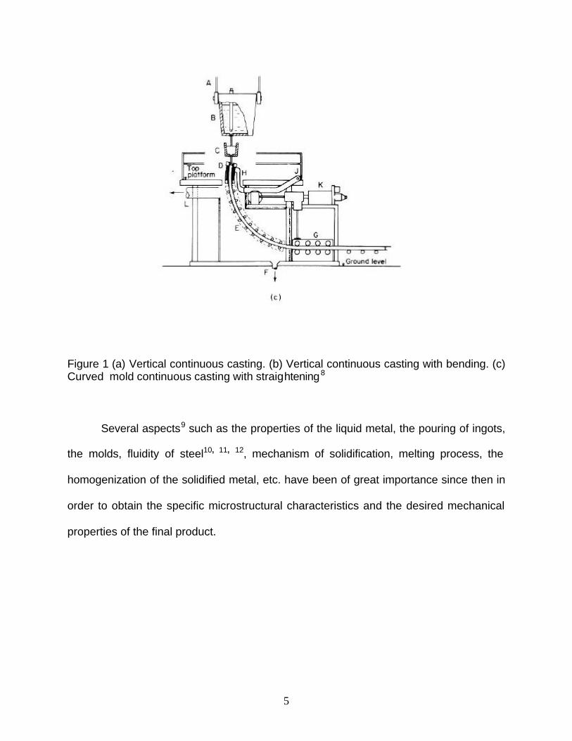
Two main types of continuous caster may be distinguished: vertical and
horizontal. The vertical is further divided into straight vertical, vertical with bending, and
curved mold with straightening- Figure 1 a, b, and c respectively.
The continuous casting process consisted in feeding molten metal from the ladle
into a water-cooled vertical mold in which the ingot would solidify. The ingot, with solid
surface but still a liquid core, was forced out of the mould continuously into a zone of
secondary cooling where the final solidification occurred3.

4
5
Figure 1 (a) Vertical continuous casting. (b) Vertical continuous casting with bending. (c) Curved mold continuous casting with straightening8
Several aspects9 such as the properties of the liquid metal, the pouring of ingots,
the molds, fluidity of steel10, 11, 12, mechanism of solidification, melting process, the
homogenization of the solidified metal, etc. have been of great importance since then in
order to obtain the specific microstructural characteristics and the desired mechanical
properties of the final product.

6
2.2 MINIMILLS
An innovative manufacturing process arose in the 60’s, the Minimill Operation
(MMO). The name minimill, according to M. M. Wolf13, was applied to “…small electric
furnace operators producing a limited assortment of unsophisticated long products like
reinforcing bars, light structurals, and wire rods.”
Minimills are associated with high productivity, with operations based on energy,
materials, capital and labor savings. They have made great contributions to continuous
casting, especially concerning a low cost production by directly charging the cast slabs
to the rolling mill in a single heat to finished product size by different casting processes:
billet casting, beam blank casting, and thin slab casting. Many minimills use electric arc
furnace (EAF) for their melting process, scrap is used mostly, the refining process
occurs in a separate ladle–furnace operation, and fast cooling is involved in the casting
process followed by an equilibrating furnace where the thin slab enters and is taken to
temperatures of up to 1150 ºC. At this temperature, the 50 mm slab is charged into a 5-
6 stand finishing mill.
It is clear that the steel produced by means of the EAF makes a great difference
compared to the conventional blast furnace and the Basic Oxygen Furnace (BOF).
2.2.1 Billet Casting
The production of low carbon steel rod, rebar and small shapes by billet casting
as a near net shape casting process (NNSC) were successfully introduced after the

7
World War II. Billet casters were of vertical type or vertical/bending type14. In a time
when the steel production was mainly from open hearth furnace (OHF) 80 % and the
rest split between EAF and the Bessemer process, the EAF technology became the
most adequate in terms of temperature control which would bring about production cost
savings. In addition, the construction of tall buildings for vertical type casters was also a
complication. This led to the design and creation of the curved mold in the mid 60’s15 -
Figure 2, or alternatively the concept of strand bending with liquid core below the
mold16, 17, 18.
By developing a better billet casting mold, casting speed would be increased19
;however, in the late 80’s, the industry found it hard to connect hot direct charging-
rolling mostly due to the difficulty in matching between the casting and rolling schedule.
Figure 2 Curved mold billet caster with rigid dummy-bar15

8
2.2.2 Beam Blank Casting (BBC)
H-Beams are conventionally rolled out of large blooms, a powerful casting
machine is required to achieve this as well as considerable rolling reduction on a
blooming mill prior to section rolling requirements which do not fit well into a minimill
structure.
The introduction of the beam blank casting (BBC) in the 60’s and in the 70’s
made everything more simple, even though it was uncertain if the process would be
cost effective20.
Production of wide flange beams used to be made by the process route steel
making-ingots-blooming-finish rolling. The introduction of the continuous casting
technology made possible the production of rectangular blooms with the proper gauges.
Continuous bloom casting technology offered some advantages such as improved
quality properties of the continuous cast blooms, higher yields as it changed from ingots
to continuously cast material, and savings by avoiding the reheating of ingots and
blooming.
The near net shape beam blank sections with a very thin web of 50 mm
thickness is a major contribution to minimill operations, which then led to Compact
Beam Production (CBP).
In all cases of new installations, caster and rolling mill are closely connected to
allow direct hot charging whenever it is possible, for instance BBC , which shows a
significant impact on the cost-effectiveness of structural steel production.

9
2.2.3 Thin Slab Casting (TSC)
Through the years, solid foundations for a new promising technology were being
built. The conventional slab casting (developed by the Integrated Steelmakers) was
adopted and implemented by the minimills in the form of a Compact Strip Mill (CSM) or
a full-fledged Hot Strip Mill (HSM).
In the search of economy, steel quality, superior properties, and very importantly,
considering the environmental issues, modifications were made in the steelmaking
industry; for instance, growth of scrap melting in the EAF and the rise of minimills, iron
and steel refining in ladles, and continuous casting into semi-finished shapes.
The way was being traced for a viable, cost-effective and reproducible
technology: The Thin Slab Casting (TSC) technology based on belt casters by the
Hazlett-type primarily21.
With the goal of increasing casting speeds for a thin slab section by conventional
mold technology, SMS (Schloemann Mannesmann Siemag) built a pilot plant in
Germany. The breakthrough was achieved with the implementation of the funnel-
shaped mold – Figure 3. This evolutionary concept consisted in reducing the slab
thickness of conventional cast steel from 250 mm to 50 mm.
Based on the pilot plant test promising results, Nucor Steel Corporation decided
to commercialize the TSC process13, 22, 18, 23, 17, 24 by building a plant in Crawfordsville,
IN, USA in 1989, and later, another plant in Hickman, AR in 1992. TSC, as expected,
resulted in a cost-effective, reproducible, and flexible process by reducing the size of
the continuous casting machine and eliminating the roughing mill.

10
By the mid 90’s only two processes had reached industrial application and had
been commercially accepted: the Compact Strip Production (CSP) process of SMS and
the In-Line Strip Production (ISP) process of Mannesmann Demag Huttentechnik
(MDH), commercialized in Arvedi, Italy. Other caster builders did not remain inactive -
Table 1. Processes such as the CONROLL process, the Danieli Thin Slab Conticaster,
which rely on mold oscillation to provide the relative motion for lubrication between the
mold and the strand; and the Belt Casters, whose functionality lies in reducing friction
between the mold and the strand by continuously moving the cooling belts as fast as the
slab 25, 26.
2.2.3.1 Compact Strip Production Process (CSP)
The CSP process, Figure 4, as well as other processes had to overcome certain
problems regarding the feeding of the liquid into the mold, the geometry of the mold, its
behavior and influence on steel quality27, casting speeds, and the improvement of the
as-cast structure, where segregation plays an important role for a superior quality of the
final/rolled product18.
The CSP – SMS casting machine is of the vertical type, 5.8 m tall, with in-line
bending to a radius of 3.8 m. The mold, made of chromium-zirconium-copper with an
immerse submerged entry nozzle (SEN), oscillates at 1 Hz per m/minute of casting
speed with a stroke length of 6 mm. Alignment tolerances between the mold and the
SEN are of critical importance to avoid breakouts. The SEN has to be ±3 mm aligned
with the mold centerline and the mold must be aligned to within ±1 mm, while the roller
apron alignment is set at ±0.2 mm below the mold. The length of the cast slabs in the

11
CSP process is 45 m. They are fed directly to an in-line roller hearth tunnel furnace
(equalizing/soaking furnace). The temperature at which the slabs enter the furnace is
about 1050 ºC, which is presumed to be a critical temperature for the formation of star-
like precipitates28, 29, 30. The equalizing furnace, where the slab remains for 20 minutes
for microstructure homogenization, raises and homogenizes the temperature of the slab
to 1150 ºC prior to entering the rolling mill. The hot strip mill consists of 5-6 tandem
finishing stands preceded by a high pressure descaler.

12
Figure 3 Schematic diagram of a funnel-shaped mold in the TSC-CSP process machine
Figure 4 Overall material flow for strip production starting from a CSP caster

13
2.2.3.2 In-line Strip Production Process (ISP)
This process has the capability of casting 60 mm thick slabs. The type of mold is
a vertical-bar type with flat parallel walls. Figure 5 shows the mold and SEN especially
developed for the ISP process31. It has a vertical top section which falls into a curved
lower part with a radius of 5 m. The SEN is about 40 mm thick by 160 mm wide. After
the mold, it has in-line thickness reduction to 40 mm still containing a liquid slab core.
The reduction is applied by a set of rolls located below the mold. After the mold, the
strand passes through three pre-reduction stands, which in turn reduce the thickness to
15 mm.
In the Arvedi, Italy ISP line, the caster is connected to an induction furnace
followed by a twin mandrel coil box (Cremona Furnace) and a four stand finishing mill.

14
Table 1 Commercial scale thin slab casting plants built as of 2000

15
Figure 5 Mold and Submerged Entry Nozzle (SEN) developed for the ISP process
2.2.3.3 CONROLL Process
Slabs 70 mm to 80 mm thick are cast through a straight mold with parallel walls,
followed by in-line bending to a radius of 3 m and straightening 32.
The CONROLL process was tested at Avesta Sheffield in Sweden to produce
stainless steels at a rate of 2 to 4 m/minute and then tested for producing carbon steel
grades33. Its maximum casting speed of 3.7 m/minute was run on a trial basis at Voest-
Alpine Stahl Linz to make 80 x 1285 mm or 1030 mm carbon steel slabs.

16
2.2.3.4 The DANIELI Thin Slab Conticaster
This caster produces plate at the Saboliare plant in Italy34. It has a normal radius
of 5.5 m and a lens-shaped curved mold equipped with 180 thermocouples. Slabs of 30-
140 mm x 900 to 2200 mm can be cast at various speeds ranging from 0.5 to 6 m/
minute. The stroke length of the mold oscillation cycle is 3.5 mm with a frequency of 3 to
5 Hz depending on the slab size, casting speed and mold powder type. It has an
equalizing/induction furnace where the slabs go after the casting machine, and a four
high rolling stand preceded by a descaler.
2.2.3.5 Belt Casters
The movement of cooling belts to reduce friction between the slabs and mold
requires the special maintenance of the belts such as their special cooling and coating
to reduce belt distortion, and at the same time, slab surface defects.
The Kawasaki-Hitachi caster is of the vertical type, twin belt with a “V-bell” mouth
shape for easy liquid metal feeding through a SEN. Thin slabs from 30 mm x 800 mm to
1000 mm are cast at speeds of 10 – 12.5 m/minute through a 3,700 mm long mold
entering directly the rolling mill without any reheating in between.

17
2.3 CONVENTIONAL CONTINUOUS CASTING (CCC) VS. THIN SLAB CASTING (TSC)
Several important changes were made from the CCC process to the TSC
process to make it more attractive for the steel industry relating to the metallurgical
aspects, economy, and environmental issues. These include the almost absolute
substitution of the blast furnace (BF) and basic oxygen furnaces (BOF) used in CCC by
the electric arc furnace (EAF) for the steelmaking practice mostly from recycled scrap
and DRI leaving the coke ovens and sinter plants far behind.
One of the most outstanding advantages of the TSC technology was the
reduction in thickness from 200 – 250 mm (10 in) slabs produced by the CCC to the 50
mm (2 in) slabs produced by the TSC. But one disadvantage is the difficult feeding of
molten metal into the narrow molds which is of great importance in the CSP and ISP
processes. K. Wunnenberg18 studied the phenomena related to the applications of
narrow molds and to thickness reduction of a strand with a liquid (mushy) core. His
conclusions were that the heat transfer in a funnel-shaped mold, designed to reduce
fluctuation in the metal level by diminishing turbulence, is rather non-stationary and non-
uniform, showing a strong variation in physical contact between the strand and the
mold, but in molds with parallel, broad walls with a narrow space between them, the
heat transfer was similar to that of the CCC. It is known that a higher casting speed
increases the mold temperature, thus, it is reasonable to expect higher heat fluxes to
the mold of thin slab casters since the casting speeds are much higher. Other studies

18
were made regarding the heat flux differences between CCC molds and a twin belt
caster mold27, 35.
The thickness reduction of a strand with a liquid core is observed by the outward
bulging of the narrow sides. Longitudinal strains in the broad sides are small. Compared
to CCC, where the reduction is too large, strains are negligible. Segregation may be
present in some steel grades produced by both CCC and TSC as a result of the in-line
reduction when the casting speed is low, the reduction segment is too long and the
reduction is too large.
It was expected that the as-cast microstructure in steels produced by TSC would
be finer than that of CCC, leading to a more homogeneous distribution of
microsegregation as a result of the faster cooling rates after solidification. Experience
has shown that the austenite grain size remains large, from 800 ? m to 1000 ?m on
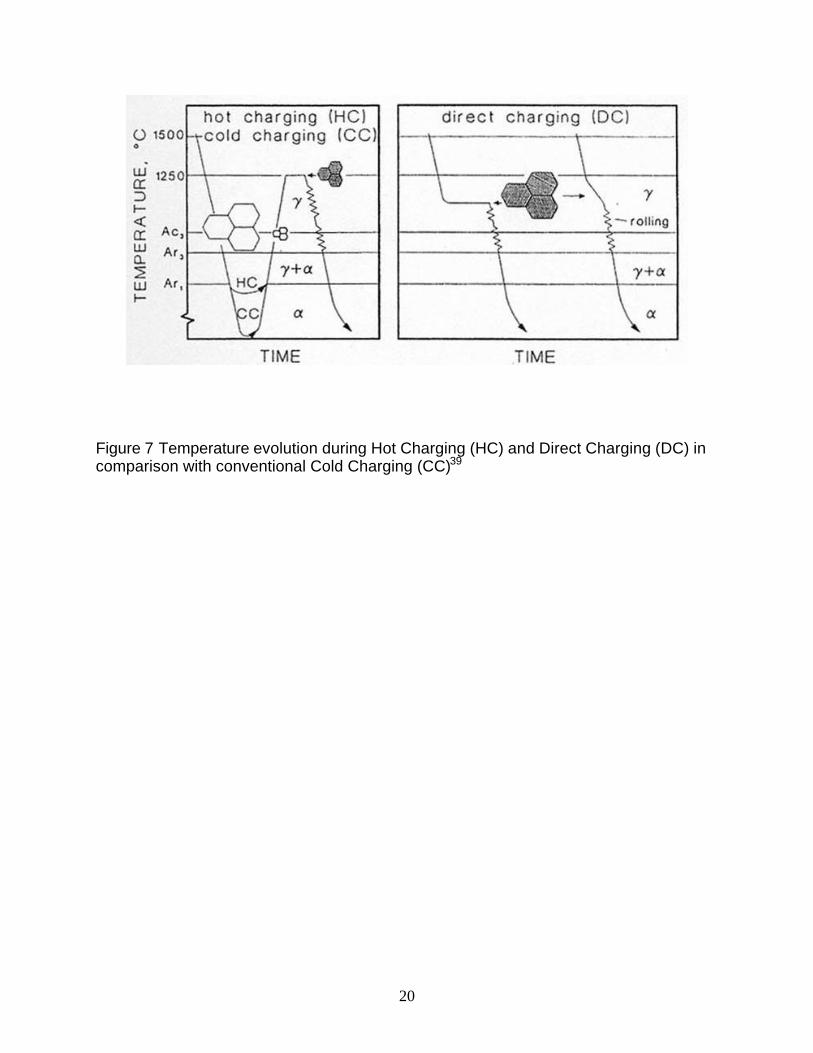
average, compared to the 200 - 300 ? m in conventional cold charge, Figure 6. The
austenite grain size of TSC is much larger than that of CCC (cold charging) after the
reheating of the slab from room temperature, Figure 7, since it does not go through any
? to a transformation during cooling and is then reheated from a to ? to provide grain
refinement as it occurs in conventional slab-reheating. The homogenization of the
original dendritic/solidification structure and the austenite grain refinement has to be
taken care of during the equilibrating furnace and the rolling process.
Other studies on TSC but with different compositions, for instance, the
simulations of a V-Nb and a V-Nb-Ti TSC microalloyed steels show the D? = ~1000 ?m
29; and a vanadium microalloyed steel, reported a D? of ~ 1000 ? m 36.

19
C M Sellars et al.23 reported that the austenite grain size (D? ) in a thin slab is 550
- 600 ?m as compared to a thick slab where it is 1000 ?m. The unavailability of the
transformations that take place during the cooling and reheating cycle and the roughing
mill before the finishing stands, are a signal of a coarse-grained as-cast structure. They
also showed other austenite grain sizes ranging from 540 ?m in the center of the slab
up to an average length in the columnar (longitudinal) zone of 2820 ?m. These data
come from a simulation test based on replacing the steel by a similar material with a
characteristically stable austenite structure over the range of temperatures from freezing
to room temperature. In addition to this, the secondary dendrite arm spacing (SDAS)
reported from this material is ~ 24 – 32 ?m. The values reported here are nowhere
close to the typical values of a commercial HSLA steel produced by the CSP process,
where the D? ranges from 600 to 1000 ?m, and a SDAS that goes from 50 to 150 ?m,
as mentioned above and in agreement with other publications elsewhere 37, 56.
Figure 6 As-cast austenite grain size distribution in an industrial thin slab sample 38
20
Figure 7 Temperature evolution during Hot Charging (HC) and Direct Charging (DC) in comparison with conventional Cold Charging (CC)39

21
2.4 AS-CAST/SOLIDIFICATION STRUCTURE
In most casting and ingot making processes, heat flow is not at steady state.
During the process of pouring liquid metal into a mold, at different locations of the mold,
for example, the metal-mold wall interface, the specific heat and the heat of fusion of the
solidifying metal go through a series of thermal resistances. As the solidification rate
depends on the thermal properties of the mold, some casting processes employ
insulating molds. For example, sand casting and investment casting 40, 41, 42, 43.
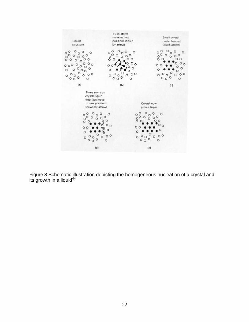
The formation of a crystal from a liquid is a homogeneous nucleation and growth
process, Figure 8. Both nucleation (N) and growth (G) rates involve atom motion which
is proportional to exp(-Q/RT), where Q is the activation energy for the atom to move, R
is the ideal gas constant and T is the absolute temperature. Both N and G are central
for controlling the rate of crystallization44 . For small undercooling, the thermodynamic
driving force is small; hence, the rate of crystallization is low. As the temperature
decreases, this driving force increases by becoming more negative, hence, the rates of
nucleation and of growth increases. Eventually this is overcome by the atom mobility.
The rates of nucleation and growth are a maximum at an intermediate temperature, as
will the rate of crystallization, Figure 9. If the cooling conditions fell below the maximum
of the crystallization curve, a metastable liquid would be obtained.
22
Figure 8 Schematic illustration depicting the homogeneous nucleation of a crystal and its growth in a liquid44

23
Figure 9 Schematic illustration of the temperature dependence of (a) the nucleation rate, N, and the growth rate, G, during solidification, (b) crystallization rate, which depends on both N and G.44
In commercial alloy casting in molds, where heterogeneous nucleation occurs,
the rise of the nucleation rate with temperature below the freezing temperature
increases at such a rate that even rapid cooling is not sufficient to prevent nucleation.
G
N
Tem
pera
ture
Nucleation rate N and Growth rate G
0ºK
Melting temperature
0ºK
Tem
pera
ture
Crystallization rate
(a) (b)

24
2.4.1 As-Cast Grain Morphology and Size
Atoms attach onto the crystal surface at different rates depending on the
crystallographic directions. In many cases, the crystal will develop a certain geometric
shape; for example, a dendrite where the crystal develops side arms or branches Figure
1041, 42, 43, 45. As the nucleation rate, (N), increases and the growth rate, (G), decreases,
a small grain size is obtained upon cooling. It is desired to have a high nucleation to get
a smaller grain size If the conditions are contrary, then few nuclei form before complete
crystallization is achieved. Hence a large grain size is obtained. The ratio of the N and
G controls the final grain size. If the temperature gradient is high, a crystal growing from
a cold mold wall tends to form an elongated shape called columnar grains. If what is
desired is a nicely formed equiaxed and fine-grained structure, the liquid can be
inoculated with fine crystalline particles of high melting point materials to act as
heterogeneous crystallization nuclei in the material upon casting.

25
(a)
(b)
Figure 10 (a) Photograph of a large, 9 in. long dendrite formed in a steel 46 and (b) schematic illustration of a dendritic crystal47.
2.4.2 Macrosegregation
Many of the solidification phenomena, structural features and macrosegregation
patterns in continuous casting of steel are similar to ingot casting if one measures time
with respect to a reference frame that moves with the strand. Axial segregation and V
Increasing time

26
segregates may be seen in longitudinal sections of continuously cast steel, whose
typical segregation occurs in the centerline of a slab.
Figure 11 Macrosegregation in a killed steel ingot. + denotes regions of positive segregation; - denotes regions of negative segregation40
Macrosegregation refers to variations in concentration that take place in alloy
castings or ingots and range in scale from several millimeters to centimeters. The scale
of chemical inhomogeneity is much greater than the dendrite arm spacing compared to
microsegregation, where the scale is smaller, usually the size of the dendrite arm
spacing. Such variations can have a detrimental impact on the subsequent processing
behavior and properties can lead to rejection of cast components or processed
products.

27
The amount of solute and location of macrosegregation in ingot casting depend
on the material’s phase diagram and the solidification process applied. Figure 11 shows
a schematic diagram of the macrosegregation in a steel ingot. During the solidification
of alloys, there is macrosegregation of solutes leading to concentration gradients from
the surface of the cast material to the center. Figure 12 shows this phenomenon for a
binary alloy containing X0 solute content, where the first solidified material will have a
composition X1. As the material solidifies through the thickness, the composition
increases until the solute content varies across the crystal and into the liquid.
When two growing crystals from opposite walls approach one another at the
centerline of the ingot, the final liquid between these two crystals is rich in solute. This is
true for conventional continuous casting (CCC), where the sections to be solidified are
relatively thick (250mm). In CCC, it has been observed that the segregation at the core
of the solidifying material is higher than that at the surface or sides.

28
Figure 12 Schematic illustration of the origin of gross ingot segregation48

29
Figure 13 Sketch of typical grain morphology in cast steel showing characteristic macrostructure: outer chill zone, columnar zone and an equiaxed zone at the center of the ingot49
2.4.3 Dendritic Segregation
The process of dendritic segregation is known as “coring”. During the equilibrium
solidification process of a pure material, the melt freezes to a single crystalline phase
which will have the same composition as the parent liquid phase. However, when
referring to alloys, solidification takes place over a range of temperatures. The
composition of the first solidified crystals is different from that of the parent liquid phase
composition, although it will be the same after further cooling until the freezing is
complete. In equilibrium cooling, the cooling rate has to be sufficiently low and the

30
motion of atoms fast enough for the composition to be that of the parent liquid
everywhere in the solid.
Coring or dendritic segregation appears due to fast cooling rates where atom
diffusion is not fast enough to reach equilibrium, giving rise to a concentration gradient
between crystals, hence, the formation of the cored structure is not an equilibrium
process. Figure 14 shows a schematic illustration of the formation of a dendrite. The
material was cut along the main dendritic axis. In order to clearly see the segregation
between the dendrite arms, the microstructure has to be properly etched50 51.
The etchant has to be such that it brings up both the solute rich-regions (dendrite
pools or zones of depression) and the solute -poor regions (zones of elevation) with a
different texture or relief.

31
Figure 14 (a) Schematic illustration of the surface topography developed upon etching in which dendritic segregation exists. Solute rich and poor regions are seen. (b) The appearance if the plane of cut is such that the ends of a dendrite arms are viewed44
Figure 13 shows a typical as-cast grain structure, a chill zone at the metal-mold
interface, a columnar-grain structure and an equiaxed zone in the center. These three
zones can be seen in castings and ingots of real materials, especially in plain carbon or
low-alloy steel. In stainless steels, the equiaxed zone does not appear, it is all columnar
with a little chill zone.
In steels, nuclei form on the walls of molds and start growing dendrites normal to
the heat flow direction in the walls. The dendrite is dependent on the degree of
undercooling as is the dendrite arm spacing, which is smaller closer to the chill zone
where the dendrite crystals nucleated. Hence as the dendrites grow, their spacing will
(a) (b)

32
change depending on the undercooling - Figure 15. The center of the dendrite arms
form first during freezing. These regions will be relatively low in carbon and alloying
elements. The interdendritic regions will be the last regions to freeze and hence, will be
solute-rich regions. In low carbon steels, the center of the dendrite may be all ferrite and
the interdendritic regions are almost all pearlite. The firstly formed dendrites are delta-
ferrite, which then transform to austenite and still later to ferrite and pearlite.
Figure 15 Data showing the increase in dendrite arm spacing as the distance from the cold mold wall increases52
A measure of the effects of solidification conditions in dendrite structures is the
Dendrite Arm Spacing (DAS) i.e., the spacing between primary, secondary or higher
order branches. Generally, the spacing measured represents the perpendicular
distances between branches. The primary dendrite arm spacing is expected to depend

33
on the product of temperature gradient and growth rate GR, by analogy with the cellular
solidification spacing53. Figure 16(a) shows one example of a ferrous alloy and 16(b) for
commercial steels with different carbon contents.
Figure 16 Experimental data on dendrite arm spacings in ferrous alloys. (a) Fe-25%Ni alloy; (b) commercial steels containing from 0.1 to 0.9% C49
Secondary dendrite arm spacings (SDAS) also depend directly on cooling rate
for a wide variety of alloys 54, 53. The SDAS reported in the literature55 for conventionally

34
cast plain carbon steels of 230 mm in thickness goes from 90 ?m at the edge to about
300 ?m at the center of the slab. Some studies related to SDAS measurements carried
out in Buschutten, involving a laboratory/ pilot plant simulation of TSC material with a
thickness of 50 mm, reveals a SDAS of 45 ? m at the surface and 95 ?m at the center.
Engl et al.56, based on a simulation of TSC, found an average SDAS of 50 ?m to 160?m
from surface to center, respectively. Other TSC SDAS were reported by Sellars et al.57.
His results are not only based on a simulation of the TSC process but also on the
variation of the original chemical composition of the steel. The SDAS ranges from 24
?m to 32 ? m.
In general, the measurements of SDAS in TSC-HSLA steels reported in the
literature range from 40 ?m at the edge to 250 ?m at the center of the slab55, 56, 57,
depending on the steel compositions and simulation conditions. These appear to be
different from those of commercially produced steels. The reduction in SDAS is
attributed to the higher cooling rates near the meniscus of the thin slab caster mold.
Also, the additions of microalloying elements such as Nb and Ti in the steel seem to
have an effect on SDA spacing. For instance, N. Pottore 51 studied the effect of Nb on
reducing the width and size of SDAS during unidirectional solidification and its effect on
the austenite grain size. He found that there is a direct correlation between the
solidification boundary and the austenite grain boundary in low carbon Nb-bearing
steels.

35
2.4.4 Homogenization
The application of heat treatments is of essential importance to chemical
homogenization of as-cast steel in order to get rid of the chemical segregation
associated with the cast material and for redistributing the solute by putting it back in
solution for grain size control and solid solution strengthening during subsequent
processing. The heat treatment is usually applied in the austenite region. The primary
concern in heating up to an austenite region is to maintain a constant austenite grain
size without coarsening with the purpose of achieving a uniform structure58 prior to hot
deformation, for instance, hot rolling, hot forging, etc.
To remove the chemical segregation or cored structure caused by the rapid
cooling rate, and due to the composition gradients along the crystal structure, the solute
atoms would have to diffuse to equilibrate or homogenize the structure, where very high
temperatures are required.
2.5 MICROALLOYED STEELS
Typical microalloyed steels are known as ferrite-pearlite low carbon-manganese
steels. They usually contain low amounts of carbon (0.1% or less) and small amounts of
carbide or nitride forming elements such as Nb, Ti or V. The combination of the alloying
elements with controlled rolling and coiling practices leads to the production of alloys
with fine grains and subgrains as a result of the formation of fine strain induced

36
precipitates in the form of carbides or nitrides, which form on the grain or subgrain
boundaries59, 60, 61. The addition of each one of these contributions mixed with the fine
grained-microstructure lead to a great increase in strength and ductility in steels. Coarse
precipitates, low volume fraction and large interparticle spacings may be detrimental to
the properties of the material.
2.5.1 High Strength Steels
The automobile market has forced the steel industry to change from low to higher
strength steels produced by cold rolling, being an effective way of strengthening when
the limit of formability is low enough for these steels to be accepted. Other high strength
steels were cold-rolled and annealed, produced initially as microalloyed hot rolled steels
with a modified chemistry to meet specific strength requirements after annealing. The
yield strength (YS) of these steels (up to 400 N/m2) were strengthened mainly by grain
refinement and were more formable than the steels with a higher degree of temper
rolling, but with lower r values. The next step would be minimizing the loss of formability
with increasing strength. As a consequence, substitutional solid solution strengthened
steels were developed, mainly because the loss of elongation per unit strength increase
is less for a solid solution strengthened steel than for a microalloyed steel, Figure 17.
These relationships are similar to those for n (work hardening) value, Figure 19.
37
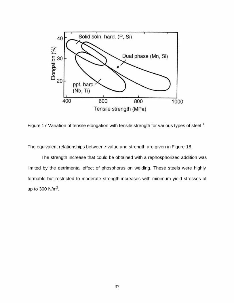
Figure 17 Variation of tensile elongation with tensile strength for various types of steel 1
The equivalent relationships between r value and strength are given in Figure 18.
The strength increase that could be obtained with a rephosphorized addition was
limited by the detrimental effect of phosphorus on welding. These steels were highly
formable but restricted to moderate strength increases with minimum yield stresses of
up to 300 N/m2.

38
Figure 18 Relationship between r value and tensile strength1
Figure 19 Relationship between n value and tensile strength62

39
2.5.2 Dual Phase Steels (DP)
Dual phase steels are low carbon HSLA steels (0.05 – 0.02% wt) that contain
Mn, Si, and microalloying additions. They have tensile strengths of up to 600 N/m2 and
show high n values but low r values as a result of their dispersed martensite islands in a
soft ferrite matrix. This occurs because of the severe cooling and intercritical annealing,
but they often still contain small amounts of retained austenite 63. The intercritical anneal
can follow either finish rolling for hot strip product or cold rolling for cold rolled and
annealed (CR&A) or hot dip galvanized (HDG) product.
2.5.3 Bake Hardenable Steels
Carbon in solution in these steels increases their yield strength up to 300 N/m2
during the baking treatment after painting and have the formability of a low-strength,
solid solution strengthened steel, but the performance of a much higher strength steel.
They are often ULC (ultra-low carbon) grades, resistant to aging at room temperature
but not at slightly elevated temperatures, especially after deformation.
40
2.5.4 Interstitial Free Steels (IF)
Interstitial free steels require additions of Nb, Ti, and V as carbide forming
elements in order to stabilize the interstitial elements. Vacuum degassing is used to
reduce the interstitial levels to ~20 ppm. IF steels are affected by secondary cold work
embrittlement. Phosphorus is added to give the material higher levels of strength, and to
reduce the harmful effects of phosphorus, boron additions are required64. The typical
tensile strength of IF steels is 440 N/m2, which is considered low-moderate, but still with
excellent formability59.
2.5.5 Transformation Induced Plasticity Steels (TRIP)
Transformation induced plasticity or TRIP assisted multiphase steels contain
small volume fractions of retained austenite in a ferrite-bainite matrix. The retained
austenite improves ductility by transforming or “tripping” to martensite under the action
of a forming strain giving rise to great crash resistance, dent resistance and weight
reduction. They reach strengths of up to 800 N/m2. TRIP steels have a high n (work
hardening) value, providing high elongation (stretch formability to the steel, and have
the potential for other forming applications such as deep drawing, where high r values
are required.

41
2.5.6 High Strength Low Alloy Steels (HSLA)
HSLA steels have been developed and produced for the last 50 years as a result
of the economic use of MA elements, which are combined in different amounts to
optimize the HSLA steels properties. HSLA steels have yield stress values from 300 to
600 N/m2 65. The upper limit of such a potential yield stress range is usually lower for a
CR&A product depending on the processing.
The MA elements, depending on the kinetics of formation of the carbides or
nitrides as precipitates and their solubility in austenite and ferrite, will have different
effects58. Cuddy et al.66 reported that alloying elements such as Al, Nb, Ti, and V initially
dissolved in austenite increase the recrystallization temperature, below which, the
application of deformation will result in fully-pancaked austenite grains, whereas
deformation above this temperature will show the presence of partially or fully
recrystallized grains. DeArdo et al.67 studied the effect of Nb supersaturation in
austenite, as it applies to the precipitation potential of Nb (CN) on the suppression of
austenite.
Figure 20 shows some of the effects that MA elements can have on austenitic
grain growth during reheating. The left side of the hatched region of the curves
represents the suppression of the primary grains. The hatched region is the temperature
at which grain coarsening (Tgc) takes place. During this transition, there is a mixture of
primary and secondary grains, and to the right side of the hatched region,
recrystallization will be present. As we can see, NbC or TiN formed at high
temperatures suppress the austenite grain growth. Nb has proven to be more effective

42
than vanadium due to its affinity for nitrogen, but TiN has a much higher effect on
austenite grain size control.
Figure 20 Austenite grain growth characteristics in steels containing various microalloy additions68
The addition of Ti to HSLA steels leads to the formation of relatively coarse
complex carbo-nitrides which may be able to reduce austenite grain growth at high
temperatures due to its solubility properties, but not the recrystallization69. Some of the
solute held as precipitate is dissolved back into solid solution during the reheating
process and may lead to further strain-induced precipitation on cooling during hot
rolling, retarding austenite recrystallization. When the final rolling is at a sufficiently low
temperature, Tstop, the recrystallization has been completely inhibited. The non-
recrystallized austenite transforms to a very fine-grained ferrite. The final ferrite grain

43
size depends on the cooling rate after the steel leaves the last finishing stand. Figure 21
illustrates how the recrystallization stop temperature differs as we increase the amounts
of MA elements. A significant variation can be seen from the great effect that Nb has
compared to Ti, Al and V which have a smaller effect respectively.
Figure 21 Effect of microalloy solute content on the recrystallization stop temperature (Tstop ) in a 0.07C, 1.40 Mn and 0.25 Si steel70
During or after the ? to a transformation, fine precipitates contribute to higher
strength levels. However, precipitates that formed in austenite do not contribute to the
strengthening of the final hot rolled structure. CR&A may be used to give the steels
improved properties by applying the proper cold reduction to the material and heat
treating it either in continuous or batch annealing 71, 72.

44
HSLA steels have, in general, a beneficial combination of high yield strength and
low temperature toughness mainly from the extremely fine-grained microstructure
coming from the phase transformation, which underwent a high degree of deformation
below Tstop.
2.5.6.1 Compact Strip Production for HSLA Hot Strip
In the last decade, The CSP technology has shown some diversification in the
product mix. One example is the production of HSLA hot strip steels, which show high
strength accompanied by excellent ductility even at low temperatures. It is considered a
value-added product in spite of the strict specifications it has to meet to be produced by
CSP. Some properties required from HSLA hot strip are high strength at static and
dynamic loads, high resistance to brittle fracture, especially at low temperatures, and
good weldability73. Several process specific characteristics have to be observed for CSP
plants which require further consideration of the following topics: a) influence of
microalloying in the microstructural evolution, b) utilization of the hot deformation to
condition the austenite and c) peculiarities of the ? to a transformation reactions 74, 75.
The conventional HSLA hot strip production is based on conventional processing
that solidifies as d-ferrite and undergoes the following phase transformations in the path
of cooling and subsequent reheating (prior to hot rolling):
Liquid –> d-Ferrite –> Austenite-?1 –> a-Ferrite –> Austenite-?2

45
In the CSP process, only the following phase transformations take place:
Liquid –> d-Ferrite –> Austenite-?1
This is due to the direct entry of the cast slab to the tunnel furnace, which is preheated
at 1150 ºC. Zajac et al. 76 and Bleck et al. 77 determined that the CSP product from
direct charging shows a higher efficiency regarding the solubility of carbonitrides in the
austenite compared to conventional cold or hot charging.
2.6 PRECIPITATION IN STEELS
Microalloying elements (MAE) such as Nb, Ti and V play a very important role in
the processing of steel. The combination of these MAE with interstitial elements such as
C and N leads to the formation of carbides or nitrides; for instance, (VC), (VN), (NbC),
(TiN), etc., or even complex carbonitrides like (Nb, Ti)(CN). These precipitates have a
strong influence on the control of the microstructure and the final properties of the steel
in different ways - Figure 2278. Depending on the temperature and processing stage at
which they form during the process, or more specifically, the recrystallization
temperature of austenite, the temperature at which the transformation occurs in addition
to other features like their size, volume fraction, and inter-particle spacing, these
precipitates will have a different effect on the properties of the material.

46
The strengthening of steel derived from microalloy additions may be produced by
the dispersion of fine precipitated particles or by grain refinement, i.e. inhibition of grain
growth by second phase particles or by a combination of both.
To obtain a fine ferrite grain size in the final product, the control of the austenite
grain size is required prior to the transformation, although the final grain size may be
greatly influenced by the control of grain growth during the ? to a transformation.
Austenite grain size is controlled by particles with high dissolution temperatures or
stable at high temperatures such as TiN and NbC.
To produce dispersion strengthening, fine particles (3-5 nm in diameter) should
be present either as interphase precipitates or precipitated after the transformation,
which is even more effective.
The understanding of the factors controlling the dissolution of the precipitates in
the form of carbides, nitrides or carbo-nitrides, is fundamental to know the effect they
will have.

47
Figure 22 Effect of microalloy precipitates on the microstructure of steel78
2.6.1 Solubility Product
Considering the reaction between a microalloying element, M, with an interstitial,
X, both being dissolved in austenite and forming a compound, MX, at a certain
temperature T
[M] + [X] ? (MX)………………. (1)
Where [M] [X] are the concentrations of M and X dissolved in austenite respectively,
and (MX) is the constituent. The equilibrium constant, referred to as the solubility
product, is obtained in terms of the activities:
Ks = a[M] * a[X] / a(MX)………………..(2)

48
It can also be expressed in terms of the elemental concentrations and activity
coefficients (? ) through
a[M] = ? [M] [M] …………………..(3)
This gives
Ks = ?[M] [M] * ?[X] [X] / a(MX)…………..(4)
assuming that the activity coefficients and the activity of the MX are equal to unity,
provided that the activities are directly proportional to the weight percentages, as they
usually are at the very low concentrations in microalloyed steels, Ks is of the form:
Ks = [M] [X]………………………..(5)
The temperature dependence of the solubility product is expressed by an equation of
the Arrhenius form:
ln Ks = -(Q/RT) + c………………….(6) or
Log10 Ks = - (Q/2.303RT) + c/2.303…...(7)
Where Q is the heat of diffusion and R is the gas constant.
A more condensed way to express equation (7) is:
Log Ks = A – B/T………………. (8)
where A and B are constants for a determined system, Log Ks is the logarithm to the
base 10, Ks is defined by equation (5), [M] [X] are expressed in weight percentages
(wt %) and T is the absolute temperature (K).
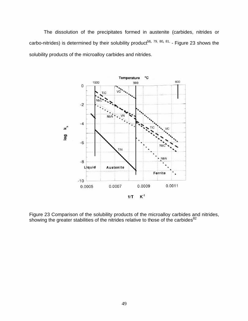
49
The dissolution of the precipitates formed in austenite (carbides, nitrides or
carbo-nitrides) is determined by their solubility product58, 79, 80, 81, - Figure 23 shows the
solubility products of the microalloy carbides and nitrides.
Figure 23 Comparison of the solubility products of the microalloy carbides and nitrides, showing the greater stabilities of the nitrides relative to those of the carbides82

50
Of particular attention is the very low solubility of TiN in austenite and the very
high solubility of VC in austenite. The solubility for carbides and nitrides in ferrite are
lower than in the austenite at low temperatures (ferrite region).
Table 2 Diffusion data for microalloy and interstitial solutes in austenite and ferrite. Also the diffusion coefficients at 1200ºC and 700ºC 83

51
Table 3 Molar volumes of microalloy carbides and nitrides based on room temperature lattice parameters84
In addition to this, there are wide variations among the different carbides and
nitrides that can be exploited. For example, in austenite, the most soluble carbide is VC,
and, as a result, it can form a higher volume fraction of precipitates on cooling and
result in more precipitate strengthening. NbC, however, is able to provide more effective
boundary pinning because of its stability as a precipitate at more elevated temperatures
than VC, where it would be in solution. However, TiN, which has the lowest solubility of
all carbides and nitrides, is more likely to remain out of solution than NbC or TiC at high
temperatures, hence, being a more effective agent (fine particles) in controlling grain
growth at very high processing temperatures by pinning the austenite grain
boundaries85. In general carbides dissolve at temperatures lower than the nitrides.

52
As the concentration of MA elements and C and N vary in HSLA steels, their
degree of solubility varies, also. Carbides and nitrides have a high degree of mutual
solubility, and, as a result, more than one metal (Nb, Ti, V) and both interstitials C and N
can be present in the precipitates which form during processing 86, 87. Complex mixtures
of solute elements with carbo-nitrides have been found in HSLA steels 88, 89, 90.
The rate of particle dissolution under isothermal conditions, when the dissolution
process is controlled by diffusion, has been calculated by means of numerical
methods91, 92.
Solubility helps to determine the rate of coarsening, which affects the force with
which these precipitates can pin the grain boundaries and dislocations. Nitrides forming
at higher temperatures are more resistant to coarsening from the equivalent carbides.
Honeycombe et al.93, found that the coarsening rate is considerably reduced by
replacing carbon with nitrogen in the precipitates or in the composition. A similar trend
occurred when the alloys were modified to replace some of the vanadium with titanium
in the precipitates94.
By having the appropriate solubility information, sufficient MA element, carbon
and nitrogen, to give the correct stoicheometric ratio, the goal would be to get the
highest solubility possible at the highest temperature involved in the controlled rolling
process.

53
2.6.2 Precipitation in HSLA Steels
Minor additions of MAE (Nb, Ti, V) and an efficient processing schedule have
resulted in tougher and stronger steels in view of the major effect of grain refinement on
both mechanical properties, yield strength and toughness.
Precipitation of carbides or nitrides of Nb, Ti or V, in austenite (f.c.c) occurs as
the temperature is decreased during controlled rolling of microalloyed steels. These
stable precipitates possess the f.c.c. structure, also. Precipitation occurs in several
ways: on grain boundaries, on dislocation networks and inside the grains or dispersed in
the matrix, and the purpose of their formation is to control recovery and recrystallization
and to inhibit austenite grain growth.
During the ? to a transformation, the presence of alloying elements can
substantially influence the phase transformation kinetics and, hence, the morphology of
the ferritic product.

54
3.0 STATEMENT OF OBJECTIVES
The objective of this work is to conduct a systematic microstructure
characterization of two different microalloyed HSLA steels (B and E, low and high Nb
and Ti contents respectively) commercially produced by the Compact Strip Production
(CSP) process in a Thin Slab Casting (TSC) plant.
Conduct a complete characterization of precipitates formed during the as-cast
and as-equilibrated processing stages of the steel.
An in-depth study of the kinetics of dissolution/formation of star-like precipitates
is made in order to understand the behavior of the precipitates in the CSP process prior
to and after the tunnel furnace.
The aim is to gain fundamental understanding of the microstructure evolution and
precipitation behavior during the as-cast and as-equilibrated process stages, in order to
increase the process efficiency in terms of microalloying content in the steel.

55
4.0 EXPERIMENTAL PROCEDURE
4.1 MATERIALS SELECTION
Several commercially produced low-carbon HSLA steels were provided by
Nucor Berkeley, USA, and HyLSA, Mexico. The as-received materials were cut from
slabs produced by the CSP process. Some of them were air-cooled and the others were
water-quenched. The water-quenched steels were selected since these samples would
provide information regarding segregation, precipitation and austenite grain size prior to
and after the tunnel furnace.
Nb-bearing microalloyed steels were received as slab blocks (20 in x 6 in x 2 in). They
were cut from the heads of the cast slabs prior to and after the tunnel furnace (TF). The
complete description of the compositions and as-received conditions of the two steels
used in this study are given in Table 4, which shows the conditions at which they were
subjected prior to and after being received.

56
Table 4 Steel compositions and as-received conditions
STEEL C wt% Mn wt% Nb wt % Ti wt% N ppm CONDITIONS
B B? BEFORE TF/WQ
BT 0.059% 1.150% 0.035% 0.004% 100
BT? AFTER TF/WQ
E E? BEFORE TF/WQ
ET 0.069% 1.234% 0.063% 0.039% 90
ET? AFTER TF/WQ
4.2 METALLOGRAPHY AND SAMPLE PREPARATION
Samples were cut from 2 inch thick slabs parallel to the casting direction –
Schematic diagram 2. They were ground and polished for metallographic analysis,
etched with 2% Nital for different times to reveal their microstructures. All
microstructural observations were made under bright field conditions on a Leitz-Epivert
conventional optical microscope.

57
Schematic Diagram 1 Origin of the as-received material: As-cast condition: B and E, as-equilibrated condition, BT and ET.
T º
C
~1200
Process time (mins.)
1150 ºC-20 mins .
W. Q.
W. Q.
Liquid
~1175
~1150
12
~1050
~950
Tunnel Furnace
As cast B, E 1
2
As equilibrated BT, ET

58
Schematic Diagram 2 Location through the thickness of the steel thin slab where the samples were cut from, and regions parallel to the casting direction that were analyzed through the thickness (S – surface, QP – quarter point and C - center).
4.2.1 Vickers Microhardness
Vickers Hardness Number (VHN-500 grams) measurements were made on all
steels on locations through the slab thickness in a LECO (VHN) Vickers microhardness
tester. An increase in hardness was observed at quarter points in both as-cast steels, B
and E, where the microstructure consisted of large amounts of non-polygonal ferrite
(especially at the quarter point), proeutectoid ferrite delineating the prior austenite
grains and polygonal ferrite at the center region in lower amounts. This in turn, led us to
do a chemical analysis at the different locations through the thickness in order to look
for segregation. Slight segregation peaks were observed at quarter points but were not
S QP
C
S
QP
Casting Direction
Observed surface

59
outstanding enough as to be considered as the main reason of that hardness increase. -
APPENDIX 1. Also, VHN microhardness was measured on the as-equilibrated steels
conditions.
4.3 REHEATING EXPERIMENTS
This section includes the path followed for the reheating experiments performed
on the as-cast steels B and E. These steels were heated from room temperature up to
three different temperatures: BR and ER to1150 ºC; BR1 and ER1 to 1175 ºC and BR2
and ER2 to 1200 ºC. Steels were held at their respective temperature for 20 minutes to
simulate the standard equalizing holding time applied to slabs directly in the industrial
process. Also, the experimental conditions of an austenitized steel (EA), reheated to
1300 ºC, held at that temperature for 3 minutes and water quenched are included –
Schematic diagram 3.

60
1175 ?C-20 mins.
5
Liquid
~1200
~1175
~1150
~1050
~950
1200 ?C-20 mins.
6
1150 ?C-20 mins.
4
T ?C
Process time (mins.)
Tunnel Furnace
As-reheated
EA
ER
BR1, ER1
BR2, ER2
Std. process
4
5
6
1300 ?C-3 mins.
3
~1300
3
1175 ?C-20 mins.
5
Liquid
~1200
~1175
~1150
~1050
~950
1200 ?C-20 mins.
6
1150 ?C-20 mins.
4
T ?C
Process time (mins.)
Tunnel Furnace
As-reheated
EA
ER
BR1, ER1
BR2, ER2
Std. process
4
5
6
1300 ?C-3 mins.
33
~1300
3
Schematic Diagram 3 Experimental paths followed for the reheating experiments of as-cast steels including EA (Austenitized to 1300 ºC-3mins + water quenched).
4.4 RE-MELTING EXPERIMENTS
Steel E, whose composition is shown in Table 4, was selected for the re-melting
practice. It consisted in re-melting the material (~1540 ºC) and simulating the casting
process by casting the liquid metal in a pre-designed copper-chill mold. The mold
operated automatically. When the slab inside the mold (1 inch thick slab, representing

61
half of the slab thickness produced in the standard TSC process) reached a certain
temperature, a compartment below the mold opened and dropped the slab to be water-
quenched to room temperature.
Three melting practices were performed at Oakridge Research National
Laboratories (ORNL) in order to examine the solidification structure and the formation of
precipitates prior to entering the tunnel furnace. The steels conditions were named (1)
EM, for the steel that was melted, cooled down to 1150 ºC and then water quenched,
(2) EMT, for the steel that was melted, cooled down to 1150 ºC, held at that temperature
for 20 minutes and water quenched, and the third one, (3) EN, which was cooled down
to a lower temperature, 1050 ºC and then water quenched. Number (2) was not used.
The experimental paths followed for the re-melting and casting practices are
shown in Schematic diagram 4. Microstructural analysis including precipitation behavior
was made on the different materials at the surface and quarter point locations. OM,
SEM and TEM techniques were used for these analyses.

62
Schematic Diagram 4 Experimental paths followed for the different re-melting and casting practices of steel E.
4.4.1 Scanning Electron Microscopy (SEM)
4.4.1.1 Sample Preparation
Specimens from the different steels were cut from three locations through the
thickness (surface, quarter point and center) so as to reveal the solidification structure
after being ground and polished. The reagent used to develop the microstructure
consisted of 200 ml of aqueous solution of picric acid, 2-4g of sodium dodecylbenzene
sulfonate; 2-4ml of HCl and in some cases 0.5g of cupric chloride. For some steels (as-
Liquid
Process time (mins.)
EM As-cast
+ cooled down to 1150?C + W.Q.
1
T ?
C
~1150 Tunnel Furnace
W Q
EM
~1050 Tunnel Furnace
EN
1
3
3 EN Cooled down to 1050?C + W.Q
2
EMT As-equilibrated
+ cooled down to 1150?C + held for 20 mins. + W.Q.
2
W Q
EMT

64
Figure 24 SEM-BSE micrograph showing dendrite pools observed for segregation, the SDAS and the approximate dendrite pool spacing at the quarter point region of steel E.
180? m
90? m
100? m

65
4.4.2 Transmission Electron Microscopy (TEM & STEM)
Precipitation analysis was made on selected locations of different steels. Several
types of precipitates were found. The observations were made on a JEM-200CX
transmission electron microscope and a JEOL 2000 scanning transmission electron
microscope both operated at 200 kV.
4.4.2.1 Sample Preparation
Thin foils were prepared by cutting 1mm thick specimens from the selected
locations with a Buehler diamond disk cut off machine. These samples were ground to
~250?m, and reduced in thickness to ~50?m by severe chemical thinning. This solution
consisted of 50 ml distilled water, 50 ml hydrogen peroxide (30%) and 7ml hydrofluoric
acid.
In the final stage of chemical polishing and etching, foils were immersed in a
solution consisting of 50 ml distilled water, 30 ml nitric acid, 15 ml hydrochloric acid and
7 ml hydrofluoric acid.
Discs of 3 mm in diameter were punched and electrochemically polished at room
temperature on a Struers-Tunepol Jet polisher at room temperature and the final
thickness of the disc at the center was of ~50-100 nm. Two solutions were used. The
first solution was made up of 90% ethanol and 10% perchloric acid and the polishing
was run at 40 V and 70-90 mA. The second solution consisted of 400 ml of acetic acid
and 80 grams of Sodium Chromate. This solution was carefully prepared by dissolving
66
the sodium chromate in the acid at room temperature. Magnetic stirring was required for
1 hr. The voltage was 20 - 25 V and a current of 60 - 80 mA. The second solution
proved to be more effective for precipitate analysis. The discs were thoroughly cleaned
in ethyl alcohol before being taken to the TEM examination.
4.4.2.2 Precipitate Characterization
TEM diffraction and magnification modes were used to identify the different kinds
of precipitates present in all steels conditions. Bright field (BF) and dark field (DF)
micrographs were taken and developed. Precipitates location, type, size, morphology
and volume fraction information were obtained by this TEM technique, whereas
quantitative analysis information was obtained by means of the STEM-EDX technique.
Precipitates compositions were measured in terms of their average Nb/ (Nb + Ti)
measured ratios.

67
5.0 RESULTS
5.1 MICROSTRUCTURAL OBSERVATIONS
The microstructure observed in water quenched steels B, BT, E and ET are
shown in Figure 26 and Figure 26. These are optical micrographs showing the typical
microstructure through the thickness of a thin slab (50 mm). Pro-eutectoid ferrite can be
seen to delineate the prior austenitic grains and inside the grains there is non-polygonal
ferrite. Higher levels of non-polygonal ferrite are observed on the as-cast samples (B
and E) than in the as-equilibrated ones (BT and ET). The non-polygonal microstructure
seems to have been homogenized by the equalizing treatment. In the industrial practice,
the slab is usually held in the tunnel/equalizing furnace for 20 minutes at a temperature
of 1150 º C.
5.1.1 Austenite Grain Size
The average austenite grain size values (D? in µm) of the two as-cast steels, B
and E and as-equilibrated, BT and ET, are shown in Table 6. The D? prior to and after
the tunnel furnace seemed to be similar. The Nb content does not seem to have a very

68
strong effect. However, the D? standard deviation of steel with the higher Nb content
both before and after the tunnel furnace is lower than the lower Nb content steel.
Figure 25 Optical microstructure through the slab thickness of steel B, conditions: a) As-cast and b) as-equilibrated
100?m
100?m
100?m
Surface
Center
Quarter Point
200?m
200?m
200?m
b) After the tunnel furnace-BT a) Prior to the tunnel furnace-B

69
Figure 26 Optical microstructure through the slab thickness of steel E, conditions: a) as-cast and b) as-equilibrated.
Surface
Quarter Point
Center
200?m
200?m
200?m
200?m
200?m
200?m
a) Prior to the tunnel furnace-E b) After the tunnel furnace-ET

70
Table 5 Average prior austenite grain size as a function of CSP processing stage
5.1.2 Microhardness Results
The VHN-500g microhardness measurements through the thickness of as-cast
steels B (0.035 %Nb, 0.059 %C, 0.004 %Ti) and E (0.063 %Nb, 0.069 %C, 0.04 %Ti)
showed an interesting increase in hardness at the quarter points - Figure 27. The steel
with the higher Nb content shows higher hardness values than the low Nb steel. These
hardness values, which are higher at the quarter point than at the surface or center
locations, are more evident in steel B than E. In order to statistically determine the
validity of this variation, a non-parametric statistical test (SPSS statistical analysis
software) was performed – Appendix 1. The test resulted in no significant variation
among the quarter point peaks and the surface and center locations. This means that
Steel - Condition D? (µm)
Std. Dev.
B (as-cast) 750 458
E (as-cast) 635 255
BT (as-equilibrated) 682 516
ET (as-equilibrated) 623 339

71
even if the power were increased (power=number of statistical samples), the increase in
hardness would not vary much more. Analysis of variance software, ANOVA, could not
be used to perform this test since this kind of statistical test requires a normal
distribution or Gauss shape curve (bell shape) tendency of the data, i.e. the hardness
values at every measured point through the width of the sample and at the different
locations through the slab thickness.
VHN 500g microhardness of steels B, BR, E and ER vs. location through the thickness
185
190
195
200
205
210
215
220
225
0 1 2 3 4 5 6
S QP C QP S Location through the thickness
VH
N-5
00g
Steel E
Steel BT
Steel B
Steel BT
Figure 27 Microhardness of steels (B, BT, E, ET) as a function of location through the slab thickness.
The VHN-500g measurements values in the as-equilibrated samples (after the
tunnel furnace) were higher at one of the surfaces of the slab and decreased through
the thickness direction.
72
5.2 THE SOLIDIFICATION STRUCTURE
The characteristic solidification structures observed through the thickness of the
thin slabs of steel B and E are presented in Figure 28.
From both dendritic structures, it can be observed that the width and size of the
dendrites is smaller at the surface and increases towards the center of the slab. The
average secondary dendrite arm spacing (SDAS) was quantitatively measured and
showed an increase from surface to center on both steels. Steel B has a SDAS of 100
?m, 250 ? m, and 280 ? m, surface-quarter point-center. These sizes are larger than the
SDAS of steel E, which go from 50 ?m, 125 ?m and 240 ?m, respectively – Figure 29.
In order to compare, the plot also shows the results of SDAS measured from a
conventionally produced slab reported in the literature55.

73
Figure 28 Dendritic structures of steels B and E through the slab thickness (surface, quarter point and center)
Surface
Center
Quarter Point
200? m
200? m
200? m
E (0.063%Nb, 0.069%C, 0.04%Ti) B (0.035%Nb, 0.059%C, 0.004%Ti)

74
SDA Spacing in two steels B and E (50mm thick slabs) as compared to a 230 mm thick slab from conventional casting
0
50
100
150
200
250
300
350
0 20 40 60
Distance from slab top surface to bottom surface (mm)
Sec
on
dar
y D
end
rite
Arm
Sp
acin
g
( ?m
)
Average SDAS of Steel B(0.059%C, 0.035%Nb, 0.004%Ti)
Average SDAS of Steel E(0.069%C, 0.063%Nb, 0.04%Ti)
Average SDAS. Crosses representrespective location through thethickness of a 230mm thick slab -Flemming et. al., Metall. Plant andTech., Vol. 11, 1988, pp. 16-35
Figure 29 Secondary dendrite arm spacing (SDAS) of steels B and E as a function of the slab thickness

75
5.2.1 Segregation Analysis Results
Figure 30 Interdendritic precipitates. “Rows” distribution from the surface region of sample E (as-cast condition)
Figure 31 Interdendritic precipitates “band” distribution from the quarter point region of steel B. (Interdendritic pool)

76
SEM revealed the existence of precipitation on both steels, as-cast and as-
equilibrated conditions. Analysis of this precipitation showed the formation of three
major types of precipitates: Star-like precipitates, cuboidal, and in a lower amount and
smaller size, spherical precipitates. The presence of all these types of precipitates
appeared mostly in interdendritic regions (i.e. interdendritic pools). They mainly formed
in rows – Figure 30 - which is a typical interdendritic precipitation distribution, formed as
the liquid melt front advances towards the solidification of the melt. Solute is rejected as
the liquid solidifies forming regions of elevation and depression, the latter being the last
to solidify and the richest in solute resulting in segregation enrichment from Nb and Ti in
the Fe matrix. They also showed another type of distribution in “bands” of precipitates,
most of them star-like - Figure 31.
Mathematical modeling software, JMAT-PRO®, was used to calculate the
distribution coefficient, K, of Nb and Ti in d-Fe.
Also, the segregation enrichment factors were calculated, for both Nb and Ti.
They are in agreement with the reported in the literature95, 96.
A series of line scans was performed on as-cast steels (B and E) in order to look
for microsegregation; first, across the precipitate rows where an increase in solute (Nb,
Ti) intensity is observed as the line scan crosses the precipitates row. A solute depleted
zone is observed by the decrease in intensity at the measured spots near the precipitate
rows - Figure 32 and Figure 33.
Second, for comparison purposes between the segregation observed in steel E
and a more homogenized dendritic structure, line scan was performed on a reheated
sample of steel E (as-cast). This sample was reheated to 1300 ºC, held there for three

77
minutes and water quenched in ice-brine. This austenitized sample (EA), as expected
showed a more homogeneous intensity detection shown by the line scan across an
interdendritic pool. Figure 34, Figure 35 and Figure 36.
Third, line scans were also performed across the entire dendrite pool (from a
primary dendrite core to an adjacent dendrite core) of the two steels B and E to look for
segregation. The measured distance ranged from 120 ?m 250 ?m depending on the
pool approximate size. Steel B showed larger dendrite pools than steel E. Figure 37 and
Figure 38.

78
(a)
Intensity vs. Location
0
1
2
3
4
5
6
7
0 5 10 15 20 25
Location across the interdendritic precipitates row
Inte
nsi
ty
NbL
TiK
(b)
Figure 32 (a) SEM micrograph showing segregation of Nb and Ti across the interdendritic precipitate row. (b) EDX line scan showing the increase in intensity at the row and a decrease before and after the row (steel E)
1
20

79
(a)
Intensity vs. Location across the precipitation "band"
0
12
3
4
56
7
8
0 5 10 15 20 25
Location
Inte
nsi
ty
Nb
Ti
(b)
Figure 33 (a) SEM micrograph showing segregation of Nb and Ti across the dendritic pool precipitation “band”. (b) EDX line scan showing the increase in intensity at the band and a decrease before and after the band (steel B)
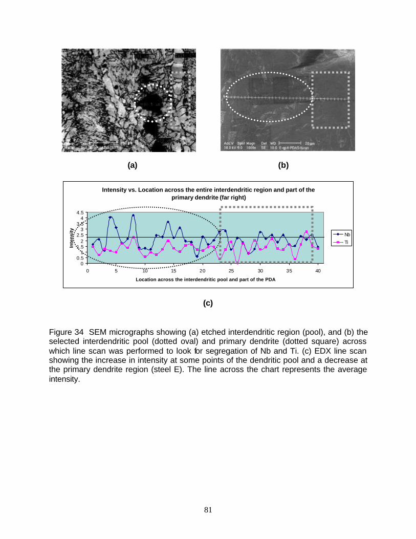
81
(a) (b)
Intensity vs. Location across the entire interdendritic region and part of the primary dendrite (far right)
00.5
11.5
22.5
33.5
44.5
0 5 10 15 20 25 30 35 40
Location across the interdendritic pool and part of the PDA
Inte
nsi
ty
Nb
Ti
(c)
Figure 34 SEM micrographs showing (a) etched interdendritic region (pool), and (b) the selected interdendritic pool (dotted oval) and primary dendrite (dotted square) across which line scan was performed to look for segregation of Nb and Ti. (c) EDX line scan showing the increase in intensity at some points of the dendritic pool and a decrease at the primary dendrite region (steel E). The line across the chart represents the average intensity.

82
(a)
Intensity vs. Location across the dendritic pool of an austenitized steel (1300 ºC and WQ)
00.5
11.5
22.5
33.5
44.5
5
0 5 10 15 20 25 30
Location across the dendrite pool
Inte
nsi
ty
Nb
Ti
(b)
Figure 35 (a) Selected interdendritic pool (dotted oval) and primary dendrite (dotted square) across which line scan was performed to look for segregation of Nb and Ti. (b) EDX line scan showing constancy in intensity through the entire interdendritic pool and parts of the primary dendrite arm - steel EA. The line across the chart represents the average intensity of steel E.

83
(a)
Intensity vs. Location across the interdendritic pool of austenitized steel E (1300 ºC + WQ)
00.5
11.5
22.5
33.5
44.5
5
0 5 10 15 20 25 30 35 40
Location across the interdendritic pool
Inte
nsity Nb
Ti
(b)
Figure 36 (a) Selected interdendritic pool and primary dendrite) across which line scan was performed to look for segregation of Nb and Ti. (b) EDX line scan showing constancy in intensity through the entire interdendritic pool and parts of the primary dendrite arm. steel EA. The line across the chart represents the average intensity from steel E.

84
(a)
Intensity vs. Location across the primary dendrite arms and interdendritic region of steel B
00.5
11.5
22.5
33.5
44.5
0 10 20 30 40 50 60
Location across the PDA and interdendritic pool
Inte
nsity Nb
Ti
(b)
Figure 37 SEM micrographs showing (a) etched interdendritic region (pool), and (b) the selected interdendritic pool (dotted oval) and primary dendrite arms (left and right dotted squares) across which line scan was performed to look for segregation of Nb and Ti. (c) EDX line scan showing the increase in intensity at some points of the dendritic pool and lower intensity at the primary dendrite region (steel B).

85
(a)
Intensity vs Location across the interdendritic pool of as-cast steel B
00.5
11.5
22.5
33.5
44.5
0 5 10 15 20 25 30
Location across the interdendritic region
Inte
nsity Nb
Ti
(b)
Figure 38 (a) SEM micrograph showing the interdendritic zone across which line scan was performed to look for segregation of Nb and Ti. (b) EDX line scan showing segregation based on the increase in intensity at some points through the interdendritic region and a decrease before and after the pool (steel B).

86
The EDX linescan analysis was performed on both steels in order to look for
solute segregation in the interdendritic regions. High amounts of precipitates were found
in the interdendritic regions compared to the dendritic regions due to segregation. EDX
line scans across the interdendritic precipitate rows and across selected interdendritic
regions (pools) were performed. The line scans show segregation in terms of the
intensity of Nb and Ti. It is observed that as the line scan crosses the row of
precipitates, an increase in Nb intensity is detected. Also in the cases where the line
scan crosses the entire interdendritic region, a higher intensity is observed than it
detects when the dendritic region is scanned. This explains the enrichment of solute in
those regions during solidification.

87
5.3 PRECIPITATE CHARACTERIZATION
The analysis of precipitates in terms of their size, type (morphology), location and
volume fraction was conducted using STEM, TEM, SEM, Image Analysis, and OM for
simpler microstructural observations.
5.3.1 As-Cast Condition
The study of precipitation for both steels B and E was conducted at the surface
and quarter point regions of the commercially produced thin slabs.
The types of precipitates observed in steel E appear in rows or randomly in the
matrix - Figure 30. They comprise three types: cuboidal TiN, star-like (Ti, Nb)(C, N), and
spherical NbC, all of which are associated with the primary solidification structure and
are a result of microsegregation.
TiN precipitates, with a typical cuboidal shape, were arranged mostly in rows.
They were found in interdendritic regions only which means they formed at high
temperatures during the solidification of the slab Figure 39. The TiN precipitates size in
steel E ranged from 50 to 80 nm with a calculated volume fraction of 1.43 x 10⁻⁵. Steel B
did not show the precipitation of TiN as much as steel E, but the sizes were much
larger. They ranged from 100-400 nm with a volume fraction of 1 x 10⁻⁶ – Figure 40. The
rest of the titanium may be distributed between the precipitates and the matrix.

88
Figure 39 (a) Bright field and (b) dark field TEM micrographs showing typical TiN precipitates (c) SEM micrograph showing general interdendritic distribution of precipitates for steel E.
100 nm
a
100nm
b
1µ m
c

89
Figure 40 TiN precipitate found in an interdendritic zone from the quarter point region of steel B – SEM micrograph.
Complex (Nb, Ti)(C, N), which precipitate mostly in interdendritic regions, contain
a TiN core and a large content of NbC. NbC precipitated epitaxially over the TiN cubes
and formed precipitates with a star-like morphology – Figure 41 and Figure 42 (a) and
(b). These star-like precipitates have a Kurdjumov-Sachs (K-S) orientation relationship
with the final ferrite which means they have precipitated in austenite 97, 98, 99. The KS
orientation relationship is obtained by the precipitates as austenite transforms to ferrite
or martensite - Figure 43. In steel E, star-like precipitates size (equivalent diameter),
measured in a BioQuant IV Image Analysis system, ranged from 80 to 160 nm and had
an estimated volume fraction of 6.2 x 10⁻⁴. The complex star-like precipitates observed
in steel B had a more symmetric shape than those observed in steel E. It showed
mostly star-like precipitation in rows or dispersed randomly in the matrix - Figure 31 and
200 nm BQP-TiN

90
Figure 42 (c) and (d). In some cases, precipitates formed in “bands” and had a
cruciform shape more than a star-like shape, with one arm more elongated than the
others – Figure 44. The cruciform shape may be an early stage in the formation of star-
like precipitates, which develop six arms instead of four. The arms are similar in
composition in both cruciform and star-like being rich in Nb at the arms. Both of these
precipitates ranged in sizes from 40 to 100 nm and a calculated volume fraction of 0.9 x
10-4.
In addition to the star-like precipitates size and morphology differences between
the two steels, their composition was also different. The average atomic ratios of
complex (Nb, Ti)(C, N) star-like precipitates in steel B (0.035%Nb, 0.004%Ti) were
0.659 in the core, and 0.735 in the arm, while in steel E the ratios ranged from 0.563 to
0.672 respectively – Table 6.

91
Figure 41 TEM micrograph of as-cast steel E (prior to tunnel furnace) showing the TiN core with the epitaxial precipitation of NbC. Also, complex (Ti, Nb)(C, N) star-like precipitates are observed.
TiN
NbC
(Ti Nb) (CN)
100 nm

92
Figure 42 TEM micrographs (left: bright field, right: dark field) showing star-like precipitates from the surface region of as-cast steels. (a), (b) Steel E and (c), (d) steel B.
b
200nm
a
200nm
d
200nm
c
220000nnmm
E
B
Bright field Dark field

93
Figure 43 Top: Star-like precipitate from the surface region of steel E (left: bright field, right: dark field). Bottom: Diffraction pattern showing the Kurdjumov- Sachs relationship between the precipitate and the matrix.
5 0 nm 5 0 nm
3-11ppt 2-20ppt
111ppt 222ppt
011 a
-131ppt
-211 a
-220ppt
-200 a

94
Figure 44 High magnification SEM micrograph showing star-like or cruciform precipitates formed in "bands", inside a selected interdendritic pool from the quarter point region of as-cast steel B.
Other types of precipitates were the spherical NbC in a much lower amount;
and, not very frequently found, needle-like precipitates. The volume fraction they
occupied was not significantly comparable to the first two types – Figure 45.

95
Figure 45 TEM bright field (a) and dark field (b) micrographs showing spherical NbC precipitated in a row, and a needle-like precipitate (not frequently found) from the surface region of steel B
5.3.2 As-Equilibrated Condition
The equilibrating heat treatment applied to the thin slabs in the tunnel furnace,
BT and ET, at 1150 ºC for 20 minutes, did not seem to affect the TiN particles observed
a
200nm
b
200nm

96
previously in as-cast material. The size of these precipitates mostly remains the same,
although there is some dissolution of the epitaxially precipitated NbC - Figure 46. On the
other hand, the star-like precipitates are affected by the temperature homogenizing
treatment by losing their initial symmetry or morphology, and, hence, decreasing in size.
The star-like precipitates observed in steel BT ranged from 25 to 50 nm in size
(equivalent diameter), whereas in steel ET their size ranged from 30 to 80 nm - Figure
47 and Figure 48 as a result of the equilibrating temperature, 1150 ºC, and the holding
time, 20 minutes.
Figure 46 TEM micrographs showing a TiN precipitate in steel BT, (a) bright field and (b) dark field images.
a
100nm
b
100nm

97
Figure 47 Partially dissolved star-like precipitates from the quarter point region of steel BT (after tunnel furnace). Also showing, rows of precipitates with a general interdendritic distribution type of precipitation as seen in the as-cast condition, steel B.
200nm
(Ti, Nb) (C, N) Partially dissolved star- like precipitates
(Ti, Nb) (C, N)

98
Figure 48 TEM micrographs showing some partially dissolved star-like precipitates; (a) bright field , (b) darkfield and (c) diffraction pattern, the last one showing the precipitates relationship to an f.c.c. matrix (Kurdjumov-Sachs). (d) and (e) show irregular shape star-like precipitates. All from the surface region of as-equilibrated steel ET.
The volume fraction calculated for steel BT was of the order 0.2 x 10⁻⁴ and their
average atomic ratios ranged from 0.68 in the center to 0.78 in the arms, while for steel
ET, the volume fraction calculated was of 8.3 x 10⁻⁵, and their average atomic ratios
were 0.575 in the core of the precipitate and 0.61 in the arms – Table 6.
200nm
a
200nm
b c
100nm
ed
100nm

99
Table 6 Quantitative and chemical analysis of star-like precipitates prior to and after the tunnel furnace
Precipitate composition
Steels
Average
precipitate
size (nm)
Volume
Fraction
(%)
Precipitate
type
Nb/(Nb+Ti)
(mol/mol)
Core - Arm
Location
E 113 0.062 (Ti, Nb) (C, N) 0.56 – 0.67 Interdendritic regions and random in matrix
ET 55 0.0083
(Ti, Nb) (C, N)
Arms Partially
dissolved
0.575 - 0.61 random in matrix
B 66 0.009 (Ti, Nb) (C, N) 0.66 - 0.74 Interdendritic regions and random in matrix
BT 39 0.0018
(Ti, Nb) (C, N)
Arms Partially
dissolved
0.68 – 0.78 random in matrix
5.3.3 Kinetics of Dissolution and Formation of Precipitates
The dissolution study of precipitates included the reheating of the as-cast steel to
higher temperatures than those of the industrial practice which is 1150 ºC for 20
minutes. The equilibrating time in the tunnel furnace remains unchanged so as to
control the number of variables.

100
The kinetics of formation involves the re-melting of one of the steels, its casting,
and water-quenching from two different solidification temperatures prior to the tunnel
furnace. This was in order to determine if the importance of the temperature control
before the slab enters the tunnel furnace, and how this can prevent the formation of
star-like precipitates at an early stage in the process. Steel E, with the higher Nb and Ti
content, is used for this practice.
5.3.3.1 Reheating Experiments - As-Reheated Condition
The first of the reheating experiments to 1150 ºC was performed to verify that the
conditions of the original as-cast steel were reproducible in terms of precipitation. The
results showed that the characteristics were fairly similar so the following reheating
experiments to higher temperatures were performed.
The reheating treatments to 1175 ºC showed the existence of TiN even after
reheating the steels to such temperatures – Figure 49. The dissolution of star-like
precipitates is observed to a higher extent than it showed in as-equilibrated conditions,
as expected. The average star-like precipitate size for steel BR1 was 13 nm and for
steel ER1, the average size was 50 nm. The evaluated volume fraction of these
precipitates in BR1 was of 2.3 x 10⁻⁶, and their measured atomic ratios ranged from 0.6
in the core to 0.7 in the arms. Regarding steel ER1, the calculated volume fraction of
dissolved star-like precipitates was of 3.16 x 10⁻⁵ and the measured atomic ratios
ranged from 0.54 in the core to 0.61 in the arms. The reheating treatments to 1200 ºC
showed, in the case of steel BR2, that all star-like or cruciform precipitates previously

101
seen in as-cast material B, had been completely dissolved, hence, the size was not
measured due to the absence of precipitates in the areas observed. In the case of steel
ER2, the average precipitate size was 48 nm and a calculated volume fraction of
0.0018% – Table 7. Figure 50,Figure 51, Figure 52 and Figure 53.
Figure 49 TEM micrographs showing TiN at the quarter point of steel BR1.
DF
BF

102
Figure 50 Dissolved star-like precipitates in rows from the quarter point region of steel BR1
Figure 51 Remains of dissolved star-like precipitates (distributed in rows) observed in the surface region of steel ER1 (TEM, left: BF, right: DF).
200 nm 200 nm
100 nm

103
Figure 52 Completely dissolved star-like precipitates after being reheated to 1200 ºC for 20 minutes (quarter point region of steel BR2).
Figure 53 Remains of dissolved star-like precipitates after being reheated to 1200 ºC for 20 minutes (from the surface region of steel ER2)

104
Table 7 Quantitative and chemical analysis of star-like precipitates for the reheating experiments (1175 ºC and 1200 ºC)
Precipitate composition
Steels
Average
precipitate
size (nm)
Volume
Fraction
(%) Precipitate
type
Nb/(Nb+Ti)
( mol/mol)
Core - Arm
Location
ER1
1175 ºC 50.5 0.0083
(Ti, Nb) (C, N)
Arms Partially
dissolved
0.54 – 0.61 random in matrix
ER2
1200 ºC 48 0.0018
(Ti, Nb) (C, N)
Arms completely
dissolved
NA random in matrix
BR1
1175 ºC 13 0.00023
(Ti, Nb) (C, N)
Arms Partially
dissolved
0.60 - 0.70 random in matrix
BR2
1200 ºC NA NA
(Ti, Nb) (C, N)
Arms completely
dissolved
NA random in matrix

105
5.3.3.2 Quantitative Analysis of Star-like Precipitates
In this section, some examples on how the measurements were performed on
the precipitates are shown.
The technique used to measure the compositions was the Scanning
Transmission Electron Microscopy (STEM). The measurements were based on atomic
and weight ratios, calculated in terms of number of counts of each element detected by
the EDX, since no method of correction was used; there was not a standard material for
reference regarding the steels accurate composition. In spite of this, the measurements
were based on the Nb-Ti ratios and the results show the effect of all the heat treatments
on both steels.
It is important to mention the following considerations for the STEM-EDX
analysis:
• Precipitates analyzed by EDX analysis in STEM microscope were observed at
very high magnifications (up to 500 K).
• After the analysis, most of the particles were destroyed due to the beam
intensity.
• Several precipitates with similar features had to be found and analyzed, in order
to get the representative measurements of Nb/(Nb+Ti) atomic ratios of both arms
and center locations.
The results of the calculated ratios Nb/(Nb + Ti) are reported in Table 6 for as-
cast and as-equilibrated conditions, and in Table 7 for as-reheated conditions.

106
5.3.3.2.1 Steel Conditions B and BT
The analysis of star-like precipitates, for instance, the one depicted in Figure 54
and Figure 56, was made on the arms and center. The corresponding spectra to the
measured locations are shown in Figure 55 and Figure 57, respectively.
5.3.3.2.1.1 As-Cast Condition - B
Figure 54 STEM micrograph showing the locations where EDX analysis was performed on a star-like precipitate, (a) right arm and (b) center.
(b) (a)

107
(a)
(b)
Figure 55 EDX spectra corresponding to (a) arm and (b) center locations of the star-like precipitate shown in Figure 54.
Energy (keV)
Cou
nts
15105
50
40
30
20
10
0
Nb
NbNb
NbNb
Nb
Ti
Ti
EDX ResidualEDX Modeled SpectrumEDX Peak FitEDX BG CorrectedEDX
Energy (keV)
Cou
nts
15105
40
30
20
10
0
Ti
Ti
Nb
NbNb
NbNb
NbEDX ResidualEDX Modeled SpectrumEDX Peak FitEDX BG CorrectedEDX

108
5.3.3.2.1.2 As-Equilibrated Condition – BT. STEM-EDX analysis was made on
precipitates with partially dissolved arms like the one shown in Figure 56 . Analyses on
the core and arms were performed as shown.
Figure 56 STEM micrograph showing the locations where EDX analysis was performed. (a) Lower arm from quarter point region of as-equilibrated steel BT.
(a)
(b)

109
(a)
(b)
Figure 57 EDX spectra corresponding to (a) lower arm and (b) center locations of the star-like precipitate shown in Figure 56
Energy (keV)
Cou
nts
20151050
60
40
20
0
Ti
Ti
Nb
NbNb
NbNb
Nb
EDX Residual
EDX Modeled Spectrum
EDX Peak FitEDX BG Corrected
EDX
Energy (keV)
Cou
nts
20151050
30
20
10
0
Ti
Ti
Nb
NbNb
NbNb
Nb
EDX ResidualEDX Modeled SpectrumEDX Peak Fit
EDX BG CorrectedEDX

110
5.3.3.2.2 Steel Conditions E and ET. The EDX measurements were made on arms
and center as indicated in Figure 58 and Figure 60 for steels prior to and after the tunnel
furnace, respectively. Their spectra are shown in Figure 59 and Figure 61 accordingly.
5.3.3.2.2.1 As-Cast Condition – Steel E
Figure 58 STEM micrograph showing the locations where EDX analysis was performed on a star-like precipitate from surface region of steel E, (a) lower arm, (b) upper arm and (c) center.
(a)
(c)
(b)
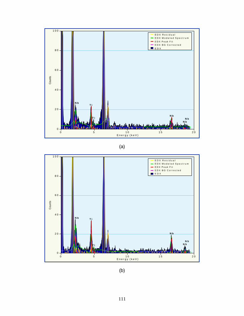
111
(a)
(b)
E n e r g y ( k e V )
Cou
nts
2 01 51 050
1 0 0
8 0
6 0
4 0
2 0
0
T i
T i
N b
N bN b
N b
E D X R e s i d u a lE D X M o d e l e d S p e c t r u mE D X P e a k F i tE D X B G C o r r e c t e dE D X
E n e r g y ( k e V )
Cou
nts
2 01 51 050
1 0 0
8 0
6 0
4 0
2 0
0
T i
T iN b
N bN b
N b
E D X R e s i d u a lE D X M o d e l e d S p e c t r u m
E D X P e a k F i tE D X B G C o r r e c t e d
E D X

112
(c)
Figure 59 EDX spectra corresponding to (a) lower arm, (b) upper arm and (c) center locations of the star-like precipitate shown in Figure 58.
E n e r g y ( k e V )
Cou
nts
2 01 51 050
1 0 0
8 0
6 0
4 0
2 0
0
T i
T i
N b
N bN b
N b
E D X R e s i d u a l
E D X M o d e l e d S p e c t r u mE D X P e a k F i t
E D X B G C o r r e c t e d
E D X

113
5.3.3.2.2.2 As-Equilibrated Condition – ET
Figure 60 STEM micrograph showing the locations where EDX analysis was performed. (a) Right arm and (b) center of a star-like precipitate (from quarter point region of as-equilibrated steel ET)
(b) (a)

114
(a)
(b)
Figure 61 EDX spectra corresponding to (a) arm and (b) center locations of the star-like precipitate shown in Figure 61.
Energy (keV)
Cou
nts
20151050
60
50
40
30
20
10
0
Ti
Ti
Nb
NbNb
NbNb
NbEDX ResidualEDX Modeled SpectrumEDX Peak Fit
EDX BG CorrectedEDX
Energy (keV)
Cou
nts
20151050
60
50
40
30
20
10
0
Ti
Ti
Nb
NbNb
NbNb
NbEDX ResidualEDX Modeled SpectrumEDX Peak Fit
EDX BG CorrectedEDX

115
5.3.3.3 Kinetics of Formation of Complex (Ti, Nb)(C, N) Star-like Precipitates
5.3.3.3.1 Re-Melting Study. The re-melting experiments applied to steel E showed that
when the steel is cast and cooled down to 1150 ºC, and water quenched to room
temperature there is no evidence of complex (Ti, Nb)(C, N) star-like precipitates, even
though the Nb and Ti contents are high.
The re-melting practice of steel E, which was cast and cooled down to 1050 ºC
and water quenched to room temperature, now named steel EN, in deed, showed the
beginning of the star-like precipitation - Figure 62. It can be observed that the arms (rich
in Nb according to the EDX measurements) of what would be a star-like precipitate
begin to grow from the core, which was Ti rich according to the EDX analysis. The
Nb/(Nb + Ti) ratio of the particle depicted in Figure 62 ranged from 0.32 to 0.50.

116
Figure 62 SEM micrographs of steel EML, showing (a) the beginning of star-like precipitates formation and (b) SEM-EDX locations for quantitative analysis.
a
1
2 3
b

117
5.3.3.3.2 CSP Thermal Simulation. Based on the results obtained in the re-melting
practice, steel E (0.063% Nb, 0.04% Ti, and 0.069% C) was selected for this
experiment. This experiment was carried out in the same research group by Y Ma110 at
the University of Pittsburgh and consisted in simulating the typical commercial CSP
process rolling schedule, but without deformation in order to identify at what
temperature the complex precipitates started to form. It is important to remark that it
was a thermal simulation only. A typical CSP process rolling schedule can be found in
Appendix 3 for reference. The experiment consisted in re-heating the steel to a
temperature high enough to make sure the star-like precipitates were dissolved. After
the reheating, the steel sample was mounted in the mechanical testing system (MTS) in
which the cooling rate, which was varied (5 ºC/s, 10 ºC/s, and 20 ºC/s) for reproducibility
purposes, could be controlled and finally water quenched the samples to room
temperature.
The results showed the initiation of the formation of new star-like precipitates, in
which NbC precipitated epitaxially on the already formed cuboidal TiN. The temperature
at which these precipitates started to form was determined to be ~1090 ºC at a cooling
rate of ~10 ºC/s. These results are consistent with the re-melting results.

118
6.0 DISCUSSION
This section is divided into 4 parts which refer to the major areas of analysis of
the two steels (B and E) commercially produced by the CSP process. The first one
refers to the microstructural characteristics of steels B, BT, E and ET including hardness
measurements through the slab thickness; the second section refers to the segregation
analysis; the third is about the precipitation behavior observed at different conditions of
both steels B and E, which includes the kinetics of formation and dissolution of the
major types of precipitates, and the fourth and last section refers to the quantitative
analysis made on these precipitates, and the effect they may have in terms of the
efficiency of Nb additions.
Other studies have been made on this type of material, but most of them are
laboratory simulations of the process, hence, there are variations in compositions and
processing conditions.

119
6.1 MICROSTRUCTURAL CHARACTERIZATION
The formation of non-polygonal ferrite was observed almost through the entire
thickness of both as-cast steels. Some proeutectoid ferrite was observed, decorating
the prior austenite grains, at the center location of the slab and in a lower amount at one
of the surfaces of the slab which is believed to occur due to the efficiency of the cooling
process, where the bottom surface is not as exposed to the cooling as is the top surface
in addition to being exposed to temperature gradients with the environment, hence
having an effect on the carbon diffusion and leading to the alteration of the
microstructure on one of the surfaces. Furthermore, the cutting and quenching
efficiency after the caster to obtain the material for the present study can have an added
effect on the formation of a non-homogeneous microstructure.
Higher levels of polygonal ferrite were observed in the as-cast steels than those
in the as-equilibrated conditions, which means that the equalizing treatment
homogenized the microstructure to a great extent; a large part of the non-polygonal
ferrite disappeared after being held in the tunnel furnace for 20 minutes - Figure 25 and
Figure 26.
Although the equalizing treatment showed an effect on the microstructure
homogenization, no effect of this treatment was observed on the prior austenite grain
size. The results are shown in Table 5. They are smaller than the ones reported in the
literature of up to ~1mm 29, 36, 38, 39, and they are in agreement with the ones reported by
Sellars et al.23, who reported D? of 500 – 600 ?m. All of these are reported from

120
simulations of the direct charging process; therefore, there are variations regarding
compositions and processing conditions.
R Kaspar and P Flub100, in a laboratory simulation, proved that the finer the as-
cast microstructure after the casting of a thin slab, the more homogeneous the micro
segregation distribution by demonstrating the effect of the rate of solidification on the
microstructure of a low-carbon microalloyed steel. The fact that the D? is coarse after
casting means that the microstructure does not have a homogeneous microsegregation
distribution, although, the prior austenitic grain sizes found in this work are smaller than
the ones they reported in a later study. Also, the D? after the tunnel furnace looked very
similar to that of as-cast steels, suggesting that the Nb content did not seem to have a
very strong effect on controlling it. However, the standard deviation of steel with the
higher Nb content, both before and after the tunnel furnace, is smaller than that of the
steel with a lower Nb content.
6.1.1 Microhardness
As seen in Figure 27, the microhardness values are higher in as-cast steel E
than in B, which was expected as steel E has a higher level of niobium than B. The
higher levels of non-polygonal ferrite were thought to have an effect on the
microhardness peaks shown at the quarter point locations on both as-cast materials, in
order to verify if the variation in hardness values at the diffe rent locations through the
thickness was significant. The statistical analysis (analysis of variance) was performed
in three ways. For the first test, S1, QP2, C3, QP4 and S5 were considered, for the

121
second test, S1, QP2, and C3 were considered, and for the third test C3, QP4 and S5
were used – Appendix 1 .
For significant variations, the statistical parameter Asymp. Sigma (AS) must
show a value of less than 0.05 (the AS value corresponding to every test can be found
on the third table of every test in Appendix 1). If the value is higher, the significance of
the difference in microhardness is not of major importance.
In the first case, the (AS) showed a value of 0.175, meaning the variation is not
significant. The same result was obtained for the second case, where only the first three
locations through the thickness were considered. The AS was 0.557, even much higher
than the first test. The third test, where the last three locations were considered,
seemed to be the closest to 0.05, with an AS value of 0.066, which means that if the
power had been higher, that is, if the number of measurements per point were
increased, the variation in microhardness may be significant.
The microhardness values in the as-equilibrated samples were higher at one
surface of the slab and decreased through the thickness direction as shown in Figure
27. This change in the overall microhardness behavior is more likely associated to the
efficiency of the quench after reheating, hence affecting the resulting microstructure.

122
6.2 SEGREGATION ANALYSIS
As shown in Figure 28, section 5.2, the dendritic structure shows an increase in
size and width from the surface and towards the center location of the slab as is
characteristic of low carbon microalloyed steels.
6.2.1 Secondary Dendrite Arm Spacing (SDAS)
The secondary dendrite arm spacings (SDAS) also increase from surface to the
center of the slab on both steels B and E used in this work – Figure 29. Steel B (low Nb
– 0.035wt %) shows higher SDAS values than steel E (high Nb – 0.063wt %) especially
at the surface and quarter point regions. The two fold difference at the surface, 100 to
200?m, and at the quarter point, 125 to 250?m, is attributed to the significantly higher
cooling rate at the meniscus of the funnel-shaped casting mold used in thin slab casting.
It is important to mention that both steels come from different sources and the
processing parameters may be different. This difference can also result from the higher
Nb and Ti content of steel E having an effect on the width and size of dendrites, and
causing the decrease in SDAS.
The SDAS in steel B are comparable to those reported by G Flemming et al. 55 of
a conventionally produced 230 mm thick slab. The surface and quarter point locations
are similar, steel B shows higher values, which suggests that either the cooling rate of B
was much slower or, more likely, the effect of microalloying elements such as Nb and Ti

123
had an effect on controlling the initial solidification structure in Flemming’s study. The
center of the thick slab shows higher values as in the regular case.
In contrast to these results, Engl et al. 56, reported SDAS from about 50 µm at the
edge of the slab to about 160 µm at the center. This study was a simulation of the TSC
and Rolling process at the Thyssen Krupp Stahl AG in Germany. Flemming’s study on a
50 mm slab (from SMS)55, reported from a laboratory test carried out at Buschhutten
pilot plant, SDAS from 50 µm at the surface, 75 µm at the quarter point and 125 µm at
the center of the slab supporting Engl’s results. The fact that these tests are based on
simulations may lead to finer SDAS by applying faster and controlled cooling rates,
which is not as easy in the regular TSC process. An example of this is the study by
Sellars et al.23, who reported SDAS from 24 µm at the edge to 32 µm at the center by
using cooling rates as low as 1 K/s and a different chemistry for the simulation by
substituting the C-Mn steel for a Fe-30Ni alloy.
6.2.2 Microsegregation Analysis
The result of the rapid solidification may be less chemical segregation and a
more homogeneous microstructure. An EDX linescan analysis was performed on both
steels in order to look for solute segregation in the interdendritic regions. High amounts
of precipitates were found in the interdendritic regions compared to the dendritic regions
due to segregation. Precipitates in both steels showed three types: 1) Complex (Ti, Nb,)
(C, N) with a star-like shape, most of them large in size. 2) Cuboidal TiN, and 3) some
small spherical NbC precipitation. These precipitates showed general interdendritic

124
distributions. They were arranged in rows or random in the matrix, in some cases, they
even precipitated in bands. These characteristics suggested a high degree of
segregation occurring in those zones. Steel E, whose Nb and Ti levels are higher than
those in B, showed higher volume fractions of these precipitates. As seen in Figures 32
and 33, EDX line scans across the interdendritic precipitate rows were performed. The
segregation is shown in terms of the intensity of Nb and Ti. It is observed that as the line
scan detector crosses the row of precipitates, an increase in intensity occurs, which
explains the enrichment of solute in those regions during solidification. Mathematical
modeling software, JMat-Pro®, was used to calculate the distribution coefficients of Nb
and Ti, and the segregation enrichment factors based on the initial concentrations and
the fractions in the solidus and the liquidus after the solidification. The JMat-Pro®
calculations for the distribution coefficients, and segregation factors are based on the
Scheil-Gulliver solidification equations. L Kuchar101 102 defined Ko as the isothermal
proportion of the admixture concentration on the solidus curve SMX , to the
concentration on the liquidus curve LMX in a binary diagram metal-admixture.
FeNbKo ?
and Fe
TiKo ?
Where,
LM
SM
XX
Ko ?

125
C is the concentration or fraction of the metal in the solidus and in the liquidus,
respectively, after the solidification.
The calculated thermodynamic distribution coefficient of Nb in d-Fe is K=0.24
with a segregation enrichment factor of ~4.3, whereas for Ti in d-Fe, K=0.25 with a
segregation enrichment factor of ~3.9. The segregation enrichment factor of Nb in Fe is
in good agreement with the one reported by L Kuchar95 of 3.75, whereas for Ti in Fe, A
Kothe et al.96 reported a segregation factor of 3. In both cases the values are higher; the
first one may be due to the model equations they based their calculations on (Brody and
Flemings Model), and the second may have been due to the fact that the segregation
factors were experimentally calculated from simulation test results; however, higher Ti
enrichment segregation factors with values of up to 9 were reported in the same study.
These were measured at spots where 3 or more microsegregation zones met.
The next step was the verification of microsegregation across the entire
interdendritic regions on both steels B and E. Figure 34, Figure 37 and Figure 38 reveal
the existence of microsegregation, shown in terms of the solute intensity peaks, which
stand out as the line scan crosses the interdendritic pool and reaches lower intensity
values as it approaches the dendrite arm.
For the verification of this behavior, one of the steels (steel E) was selected to be
austenitized to 1300 ºC for 3 minutes, in order to confirm that as the material is exposed
to higher temperatures, a homogenization of the initial segregation that took place
during solidification could be achieved. The steel called EA (austenitized) was then
especially etched to reveal the dendritic structure. The observations resulted, as
depicted on Figures 35 and 36, from the structure homogenization by showing a lower

126
and more uniform solute intensity (below the average shown by steel E) across one of
the interdendritic regions analyzed by SEM-EDX line scan.
6.3 PRECIPITATION ANALYSIS
It is important to mention that precipitation hardening was not considered in this
study, but rather, precipitation for microstructure control.
It is known that the additions of microalloying elements (MAE) such as Nb, Ti,
and V and interstitial elements such as N and C help to improve the mechanical
properties of HSLA steels by having a strong impact on the microstructure evolution
throughout the process and up to the final product. This occurs as a result of the
combination of both alloying and interstitial elements bringing about the formation of
different types of precipitates. See section 5.3.1.
The precipitation results in both steels were found to be strongly influenced by
the local enrichment of microalloying elements resulting from interdendritic segregation.
This is supported by the results found by S V Subramanian and G C Weatherly103, who
studied the degree of heterogeneity in the size and dispersion of precipitates and the
microchemistry of meta-stable precipitates in a Ti-Nb microalloyed steel. Also, C Zhou
and R Priestner28, and Engl et al.56, stated that increasing the solute above a critical
level, hence over passing a certain level of supersaturation, would lead to interdendritic
precipitation of carbo-nitrides.

127
For comparison purposes, a complete description of the quantitative
measurements results of all steels conditions consult Table 8, at the end of this section.
6.3.1 As-Cast and As-Equilibrated Conditions
In the present work, the formation of cuboidal TiN precipitates was observed in
both as-cast and as-equilibrated steels. It was found that these precipitates are
interdendritic since they form at high temperatures during solidification. These
precipitates were also observed by R Priestner et al.28 in steels containing similar levels
of Ti to steel E.
The volume fraction of these precipitates was higher in steel E, 1.43 x10⁻⁵, as a
result of its high Ti content (0.04 wt %) and the levels of segregation in the
interdendritic zones, as compared to the lower volume fraction of this type of
precipitates, 1 x 10⁻⁶, in steel B, whose original titanium content was ten times less. It
was found that in steel ET, after the tunnel furnace, that the TiN size was not affected
by the equilibrating treatment, where it was held for 20 minutes, due to its stability at
high temperatures, according to T Gladman104, the studies of the solubility of TiN have
indicated that of all the microalloy carbides and nitrides, TiN is the most stable. TiN
precipitates do not seem to grow or dissolve during or after the equalizing heat
treatment. Various dissolution temperatures of TiN in liquid and in austenite for
comparison purposes are shown in Figure 63. The TiN precipitates in steel BT showed
a decrease in size due to the dissolution of the NbC, which precipitated epitaxially on
the cuboidal TiN - Figure 40 and Figure 46. The dissolution temperature of NbC, shown

128
in Figure 64 was calculated in terms of the solubility of NbC in austenite by two authors
for comparison purposes.
While most studies agree with the size and distribution of TiN precipitates, only a
few refer to the presence of the complex star-like or cruciform (Ti, Nb)(C, N) or (Ti, Nb,
V)(C, N) precipitates before the equilibrating heat treatment28, 29, 30 and other more
recent studies105, 106.
Star-like precipitates were observed in as-cast steels, E (0.063% Nb) and B
(0.035% Nb) - Figure 42, Figure 43 and Figure 44. The volume fraction of star-like
precipitates was much higher in steel E than in B, 0.062%, and 0.009%, respectively,
which is a reflection of the steels compositions. Their morphology is associated with the
epitaxial precipitation of NbC over the TiN previously formed as it was also predicted by
S V Subramanian et al.103. Also, based on the mutual solubility shown by nitride-forming
microalloying elements such as titanium, niobium and vanadium, they may form
complex carbo-nitrides and may exist as a single constituent phase107. Star-like
precipitates in the lower Nb content steel showed smaller sizes and looked more
symmetrical than those of steel E. This could be related to the NbC precipitated
epitaxially on the TiN precipitates - Figure 41. Since steel E had much higher Nb and Ti
contents, the arms of the star-like precipitate would grow larger on a larger TiN
precipitate (core) and not as well defined as those in steel B. This can be explained in
terms of the difference in atomic ratios Nb/(Nb + Ti) calculated between the arms and
center of precipitates in both as-cast and as-equilibrated steels. The atomic ratios are
reported in Table 6 and for further comparison with other steels conditions in Table 8.
Figure 65 for steel E (all conditions) and Figure 66 for steel B (all conditions including

129
hot band observations) show the atomic ratios plotted as a function of the position on
the precipitate from all the conditions. The procedure to obtain such information is
described in section 5.3.3.2.
In steel E, the Nb/(Nb + Ti) measured ratio was 0.056 – 0.067 at the center and
arm positions on the precipitate respectively; meaning that the arms of the precipitates
were not as rich in Ti as was the center of the precipitate, the arms show a higher ratio
which meant they were Nb rich. In the as-equilibrated condition (ET), where the
precipitates were partially dissolved, the atomic ratio measured in the arms showed a
decrease, from 0.67 (as-cast-E) to 0.61 and a slight increase in the center, from 0.056
(as-cast -E) to 0.575, explaining the partial dissolution of NbC (arms) during the heat
treatment in the equilibrating furnace for 20 minutes and the exposure of the TiN core
as this occurs. A similar type of behavior was observed in steel B and BT. The ratios
measured ranged from 0.66 in the center up to 0.78 in the arms, which explains the
absence of Ti, and the probable enrichment of Nb after the equilibrating treatment,
where the average size of the precipitates decreases from 66 to 39 nm. Some small TiN
precipitates were observed as the NbC arms dissolve during the equilibrating treatment
and after reheating treatments to higher temperatures as seen on steel E. The volume
fraction of star-like precipitates in steel ET was still higher than that of BT, 0.0083% and
0.0018%, respectively, after the 20 minutes holding time in the tunnel/equilibrating
furnace at an approximate temperature of 1150 ºC-Table 8.

130
Dissolution Temperature of TiN as a function of wt % Ti
1502
1337
1425
1854
1000
1100
1200
1300
1400
1500
1600
1700
1800
1900
0 0.005 0.01 0.015 0.02 0.025 0.03 0.035 0.04 0.045
wt % Ti
Tem
per
atu
re º
C
TiN in Liquid -Narita
TiN in Austenite-Matsuda et al.
Figure 63 Dissolution temperature (ºC) of TiN based on titanium content – Two different solubility product conditions: Narita81 and Matsuda et al.85

131
Dissolution Temperatures of NbC as a function of wt % Nb
1094
1021 980
913
500
600
700
800
900
1000
1100
1200
0 0.02 0.04 0.06 0.08
wt % Nb
Tem
per
atu
re º
C
NbC-Narita
NbC-Palmiere
Figure 64 Dissolution temperature (ºC) of NbC based on niobium content – Two different solubility product calculations: Narita81 and Palmiere58
6.3.2 Kinetics of Dissolution and Formation of Star-Like Precipitates
These complex star-like precipitates (Ti, Nb)(C, N) dissolve as the temperature is
progressively increased and, according to M Prykril et al. 30, although in a different
system (Ti, V, Nb microalloyed steel), if the holding time is prolonged, in addition to the
complex carbo-nitride progressive dissolution, there is titanium enrichment.

132
6.3.2.1 As-Reheated Conditions – BR1, ER1 (1175 ºC – 20 mins.) and BR2, ER2, (1200 ºC – 20 mins.)
The increase in temperature in the equilibrating stage of the process led to
complex precipitates dissolution, however, the NbC arms of star-like precipitates in steel
ER1 seemed to reach a dissolution limit. The precipitates average size decreased from
55 nm (as-equilibrated-ET) to 50.5 nm (as-reheated to 1175 ºC-ER1). Although the
numbers seem to be fairly constant, the volume fraction in the ER1 condition,
0.00316%, and was still lower than that of the ET condition, but only by a factor of 2.6.
The Nb/(Nb + Ti) ratio in the center decreased slightly, from 0.575 (ET) to 0.54
(ER1), which means there was a gain of Nb, and remained constant in the almost
completely dissolved arms, 0.61, most likely due to the almost complete dissolution of
NbC after being held in the equalizing furnace for 20 minutes at a temperature as high
as 1175 ºC.
In the lower Nb and Ti content steel, the precipitate size decreased from 39 nm
(as-equilibrated-BT) to 13 nm (as-reheated-BR1). The volume fraction decreased from
0.0018% in the BT condition to 0.00023% in the BR1 condition. Their atomic ratios were
0.54 – 0.61 and 0.68 – 0.78, respectively. This meant that there was an enrichment of
Nb, which is somewhat similar to what was observed in steel ER1, although not as
clear, due to the presence of TiN precipitates as a result of the higher Ti content.
In the second case of as-reheated condition, steels ER2 and BR2, the same
complete analysis as with the previous conditions could not be made. It was observed
that the precipitate average size decreased slightly by only 2.5 nm, from 50.5 nm (ER1)
to 48 nm (ER2) after being reheated at a temperature as high as 1200 ºC for 20

133
minutes. The measured volume fraction of steel ER2 was, 0.00183%, decreasing even
more, as expected, but only by a factor of 1.7 as compared to the factor of 2.6 between
the ER1 and ET conditions, and a factor of 7.4 between the ET and E conditions.
Only a few TiN precipitates were observed in condition BR2, the size of some of
the few precipitates found, ranged from 20 to 100 ?m as a result of the dissolution of the
NbC that had precipitated epitaxially on the TiN. Star-like precipitates in the BR2
condition were completely dissolved; therefore, no information could be obtained about
this kind of precipitation.
The increase in atomic ratios observed in the as-reheated conditions of both
steels (ER1 and BR1) may lead to a re-precipitation of NbC and even growth and
coarsening of complex precipitates at longer equalizing holding times28, 30, 105 or during
the rolling process29.

134
Table 8 Quantitative and chemical analysis results of star-like precipitates prior to and after the tunnel furnace including reheated conditions and hot band
Precipitate composition
Steels Average
precipitate size (nm)
Volume Fraction
(%) Precipitate
type
Nb/(Nb+Ti) ( mol/mol) Core - Arm
Location
E 113 0.062 (Ti, Nb) (C, N) 0.56 – 0.67
Interdendritic regions and random in
matrix
ET 55 0.0083 (Ti, Nb) (C, N) 0.57 - 0.61 random in
matrix
ER1 50 0.00316 (Ti, Nb) (C, N)
Partially dissolved
0.54 - 0.61 random in
matrix
B 66 0.009 (Ti, Nb) (C, N) 0.66 - 0.74
Interdendritic regions and random in
matrix
BT 39 0.0018 (Ti, Nb) (C, N) 0.68-0.78 random in
matrix
BR1 13 0.00023 (Ti, Nb) (C, N)
Partially dissolved
0.60 – 0.70 random in
matrix
Hot Band-
E 150 0.060 (Ti, Nb) (C, N) 0.68 – 0.72
random in matrix

135
Atomic ratio vs. Location on precipitate - different conditions of steel E (0.069%C, 0.063%Nb, 0.04%Ti)
0.4
0.45
0.5
0.55
0.6
0.65
0.7
0.75
0 1 2 3
Arm CoreLocation on precipitate
Ato
mic
rat
io N
b/(N
b+Ti
) (m
ol/m
ol)
E as-cast
ET as-equilibrated
ER1 as-reheated to1175ºC
EHB hot band
Figure 65 Nb-Ti content distribution in star-like precipitates from different conditions of steel E, including EHB -hot band for comparison purposes

136
Atomic ratio vs. Location on precipitate - different conditions of steel B (0.059%C, 0.035%Nb, 0.004%Ti)
0.4
0.45
0.5
0.55
0.6
0.65
0.7
0.75
0.8
0 1 2 3Arm Core
Location on precipitate
Ato
mic
rat
io N
b/(N
b +
Ti)
(mo
l/mo
l)
B as-cast
BT as-equilibrated
BR1 as-reheated to1175 ºC
Figure 66 Nb -Ti content distribution in star-like precipitates from different conditions of steel B
6.3.2.2 Kinetics of Formation
The results of the re-melting analysis, when cooling down to two different
temperatures, (1150 ºC and 1050 ºC) followed by water-quenching to room temperature,
suggested the beginning of the formation of star-like precipitates takes place at a
temperature in between the two temperatures used for this practice. Based on this, Y Ma
carried out the thermal simulation at different cooling rates, cooling down to different
temperatures paying especial attention to the temperature range between 1150 ºC and
1050 ºC. The determined start or critical temperature at which these precipitates formed

137
was approximately 1090 ºC at a cooling rate of ~9 ºC/sec. Meaning that, the formation of
such complex star-like precipitates in the industrial practice occurs before the slab enters
the equalizing furnace, reaching temperatures as low as 1000 ºC.
6.4 QUANTITATIVE ANALYSIS
This section refers to the chemical analysis performed on one of the steels (as-
cast steel E). The analysis was performed at a research institute in China (CISRI). Also,
based on the Nb/(Nb + Ti) ratios measured in the present study, a mass balance was
made in order to see how much of the Nb is consumed for the formation of the complex
(Ti, Nb)(C, N) star-like precipitates and how much is still available in solution for further
processing. Results are compared to steel EHB, named after the hot band condition of
steel E. The analysis of this steel condition was performed by R Wang 108 in the same
research group (BAMPRI) at the University of Pittsburgh.
6.4.1 Chemical Analysis and Mass Balance
The chemical analysis showed that the total amount of precipitate phase in the
form of M(Cx, Ny)(wt %) constituted 0.114 wt% in steel E. Star-like precipitates
represented the 48 %, which contained Ti, Nb, C and N and constituted 0.055 wt% of

138
the total amount of precipitate phase. C and N constitute 15.8%, whereas Ti and Nb
represented 84.2% of the total.
By multiplying the 84.2 % times the calculated volume fraction of complex star-
like precipitates in as-cast steel E, 0.0618 %, the total amount of Ti and Nb in the star-
like precipitates was obtained. Taking into account the Nb/(Nb + Ti) average ratio
measured for this condition, which was 0.753, times 0.00052, which is the total amount
of Ti and Nb in the star-like precipitates, resulted in a value of 0.039 wt % of Nb, and a
0.013 wt % of Ti, representing the approximate amounts of Nb and Ti, respectively,
consumed in the formation of these complex precipitates.
It was assumed that the volume fraction of NbC is equal to the mass fraction of
the same by a factor of 1.0092109:
fv (NbC) = 1.0092 x W (NbC)
Where,
fv = Volume Fraction
W – Weight
This means there was an approximate amount of 0.024 wt % of Nb in solution for
further processing.
Taking these calculations as a reference, the approximate wt% of Nb tied up in
star-like precipitates was calculated for the ET and ER1 conditions. The results are
shown in Figure 67.

139
Other analyses for the Nb distribution in steel EHB conducted at CISRI showed
that the 0.0378 wt% of Nb was in star-like precipitates, the 0.0172 wt% was held in
other precipitates and 0.0075 wt% was still in solid solution, which corresponded to a
60%, 27.5% and 12% of the total Nb content in steel E, respectively.
It is clearly observed that the amount of Nb dissolved after the equalizing
treatment is high, and even higher dissolution levels are reached when the steel is
exposed to higher heating temperatures. Interestingly enough, this Nb that was
expectedly dissolved, is unexpectedly drawn back from the matrix to form the same type
of precipitates and even a very similar volume fraction as it can be observed in Figure
67, suggesting that the formation of complex carbo-nitride star-like precipitates takes
place either between the equalizing furnace and the rolling mill or during the rolling
process. Therefore, it is required to control the temperature at which the slab enters the
hot rolling mill or the time it takes to go inside the milling train in order to avoid the
formation of these complex (Nb, Ti)(C, N) star-like precipitates which consume the Nb at
a greater extent than expected.

140
Wt% Nb consumed in star-like precipitates (steel E - different conditions compared to the bulk)
0.039
0.0050.0018
0.0378
0
0.01
0.02
0.03
0.04
0.05
0.06
0.07
As-cast As-equilibrated As-rhtd. 1175 ºC Hot Band (108)
Steel Condition
wt %
Nb
in s
tar-
like
pre
cip
itate
s
Bulk - 0.063 wt % Nb
Figure 67 Weight percent of Nb consumed in the formation of complex (Nb, Ti)(C, N) precipitates with a star-like morphology as a function of the different conditions of steel E including the wt % Nb from the hot band stage (EHB) 108.

141
7.0 CONCLUSIONS
The equalizing heat treatment seemed to have a good effect on the
homogenization of the microstructure since the high levels of non-polygonal ferrite
observed in the as-cast structure decreased with the equilibrating heat treatment
resulting in a more homogeneous microstructure.
The VHN microhardness peaks observed at the quarter points through the
thickness of the as-cast slabs showed no sign of macrosegregation at those specific
regions.
The fact that the microhardness in the as-equilibrated condition showed higher
values at one of the surfaces and decreased through the thickness direction was
attributed to the quenching efficiency after the sample was cropped from the slab for
investigation, resulting in a microstructural inhomogeneity.
Even though the D? values ranged from 635 to 750 ?m, they were not as large
as the ones reported in the literature of 1mm in average (from laboratory simulations of
the TSC process), it could be suggested that the microstructure of the steels studied in
this work would be more homogeneous, based on the fact that a finer cast structure
after thin slab casting brings about a more homogeneous microstructure.
There is no significant effect of alloying elements such as Ti in controlling the
prior austenitic grain size D?

142
Segregation of microalloying elements during solidification was observed
reflected in the high degree of interdendritic precipitation.
The D? nucleation occurs at the d/d boundaries and its growth is controlled by
the SDAS and the presence of TiN. Microalloying elements apparently did not
precipitate as TiN interdendritically at the d/d boundaries; hence the growth control of
D? is not observed.
As the SDAS of steel E is not as large as that of steel B, we suggest that the first
steel underwent a more effective quenching treatment, since higher cooling rates lead
to more homogeneous distribution of microsegregation.
Although the effect of TiN was not clearly observed, the prior austenitic grain size
is smaller in E than in B, which suggested that the higher Ti content steel may have had
some effect in controlling D?.
Two major types of precipitates, were observed in the as-cast condition: cuboidal
TiN and complex (Ti, Nb)(C, N) star-like precipitates, which had a K-S relationship to the
matrix,. Also but not significantly, small spherical NbC and needle-shaped precipitates
were observed.
The formation of star-like precipitates occurs at an temperature of 1090 ºC.
Star-like precipitates undergo several changes after the equalizing treatment:
they reduce in size and lose their initial symmetry.
During the equalizing treatment there is not a complete precipitate dissolution.
When the steels are exposed to higher temperatures than the typical equilibrating
temperature of 1150 ºC, the arms of star-like precipitates seem to progressively dissolve
until the TiN core is reached.

143
Although the equalizing temperature treatment appeared to have dissolved part
of the NbC, the fact that it is put back in solution and stays there for subsequent
processing depends very much on the diffusion coefficient of Nb and C, and the speed
at which the slab is charged in to the hot rolling mill. The reason for this is that as the
temperature decreases, the formation of the complex star-like precipitates may take
place again consuming a high amount of the available Nb.
It was observed that the volume fraction of star-like precipitates was the same in
both as-cast and the hot band conditions of steel E. This suggested that the
temperature at which the slab was charged in to the rolling mill went below the critical
temperature for the formation of star-like precipitates, resulting in the re-precipitation of
NbC in the form of complex (Nb, Ti)(C, N) star-like precipitates epitaxially on the
undissolved TiN.
Based on the mass balance the amount of Nb consumed in the formation of star-
like precipitates is approximately the 60% of the initial concentration, which can also be
observed in the hot band condition.
The amount of Ti and N in HSLA steels produced by the CSP process has to be
optimized with the purpose of either avoiding or reducing the formation of star-like
precipitates.
Control the slab temperature (over 1090 ºC) through the casting, equalizing and
rolling treatments, in order to avoid the formation of star-like precipitates.
The CSP practice does not utilize Nb very efficiently.

144
APPENDIX 1
SPSS (STATISTICAL ANALYSIS SOFTWARE)
Proficiency with statistical software packages is indispensable today for serious
research in the sciences. SPSS (Statistical Package for the Social Sciences) is one of
the most widely available and powerful statistical software packages. It covers a broad
range of statistical procedures that allow you to summarize data (e.g., compute means
and standard deviations), determine whether there are significant differences between
groups (e.g., t-tests, analysis of variance), examine relationships among variables
(e.g., correlation, multiple regression), and graph results (e.g., bar charts, line graphs).
SPSS software was the software used for the analysis of variance in
microhardness explained in section 4.2.1.
Analysis of variance (ANOVA) spreadsheet is only used when the samples
(statistical samples) follow a normal distribution or Gauss shape / Bell-shape curve. For
this or other analysis of variance, e. g. the t-tests, the analysis can be performed, but
the power (number of samples/measurements) has to be very high, usually more than
30 per point.
When measuring microhardness (VHN), sometimes it is not possible to achieve
such amount due to the sample dimensions or the required separation between each of

145
the measurements. In the case of the steels tested for VHN measurements in this work,
neither of the requirements mentioned above was met.
Steels B and E showed an increase in hardness at the quarter point regions
through the thickness of the slab. To statistically verify the significance of the hardness
variations at those points, the use of a non-parametric test was required, that means a
test where the number of tests or the power is not a rigorous requirement. Although, as
it is the case in every statistical analysis, the higher the power, the more representative
and reliable the analysis results.
Steel B VHN microhardness curve was selected for the analysis since it was the
one that showed a more outstanding variation in hardness among the different locations
through the thickness, namely, S1, QP2, C3, QP4, and S5. See Figure 68.

146
Microhardness of steels B and E vs. location through the thickness
180
230
0 1 2 3 4 5 6
S QP C QP S Location through the thickness
VH
N -
500
g
Steel E
Steel B
Figure 68 Microhardness of as-cast steels B and E as a function of location through the slab thickness. Steel B (lower curve) was selected for statistical analysis.

147
Firstly, the SPSS analysis was performed on the five locations, S1, QP2, C3,
QP4 and S5 using the non-parametric test Kruskal-Wallis. The results were as follows:
NPAR TESTS /K-W=measure BY site (1 5) /STATISTICS DESCRIPTIVES /MISSING ANALYSIS. NPar Tests Descriptive Statistics
N Mean Std. Deviation Minimum Maximum
MEASURE 30 203.90 17.375 173 241
SITE 30 3.00 1.438 1 5
Kruskal-Wallis Test
Ranks
SITE N Mean Rank
1 6 17.00
2 6 20.17
3 6 13.50
4 6 18.17
5 6 8.67
MEASURE
Total 30
Test Statistics (a, b)
MEASURE
Chi-Square 6.344
df 4
Asymp. Sig. .175
a Kruskal Wallis Test b Grouping Variable: SITE
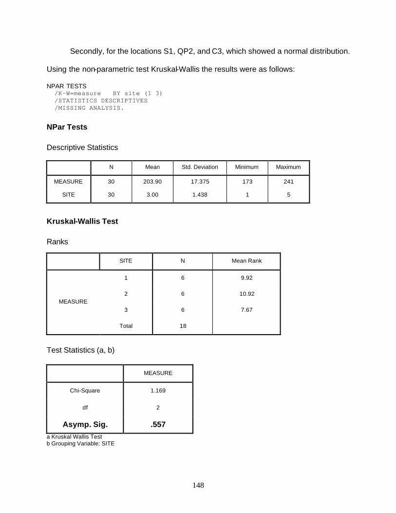
148
Secondly, for the locations S1, QP2, and C3, which showed a normal distribution.
Using the non-parametric test Kruskal-Wallis the results were as follows:
NPAR TESTS /K-W=measure BY site (1 3) /STATISTICS DESCRIPTIVES /MISSING ANALYSIS.
NPar Tests
Descriptive Statistics
N Mean Std. Deviation Minimum Maximum
MEASURE 30 203.90 17.375 173 241
SITE 30 3.00 1.438 1 5
Kruskal-Wallis Test
Ranks
SITE N Mean Rank
1 6 9.92
2 6 10.92
3 6 7.67 MEASURE
Total 18
Test Statistics (a, b)
MEASURE
Chi-Square 1.169
df 2
Asymp. Sig. .557
a Kruskal Wallis Test b Grouping Variable: SITE

149
The final statistical test included locations C3, QP4 and S5, which also had a
normal distribution and by using the non-parametric test Kruskal-Wallis, also.
NPAR TESTS /K-W=measure BY site (1 3) /STATISTICS DESCRIPTIVES /MISSING ANALYSIS.
NPar Tests Descriptive Statistics
N Mean Std. Deviation Minimum Maximum
MEASURE 30 203.90 17.375 173 241
SITE 30 3.00 1.438 1 5
Kruskal-Wallis Test
Ranks
SITE N Mean Rank
3 6 9.33
4 6 13.17
5 6 6.00 MEASURE
Total 18
Test Statistics (a, b)
MEASURE
Chi-Square 5.426
df 2
Asymp. Sig. .066
a Kruskal Wallis Test b Grouping Variable: SITE

150
APPENDIX 2
SEM – EDAX – EDX AUTO
LINE SCAN PROFILE
a. From the MAIN MENU, select EDX.
b. Click on EDX- Auto
c. Set up – preset the clock for collection times (seconds).
d. Image – collect
e. Press START to collect spectrum. To automatically show identified elements, go
to ID - AUTO
f. If you want to add other elements or subtract from the identified ones, select the
desired elements and click on add or remove/clear elements from the screen.
g. Image - collect again for EDX Auto to pull the selected image from the
microscope mode.
h. Click on LOCA-S – select Line. It will change to LOCA-L
i. Draw a line on the collected image across the desired location for analysis and
click on save icon S.
j. Go to LOCA-L again and select TABLE

151
k. Under the cell corresponding to No – X, highlight the cell and change the number
of points you want the line scan analysis along the line drawn. The default is 10,
if it is desired to run more than 10 spots along the line, change to X number and
click on copy icon C, click OK to return.
l. Click on LOCA-L, select Show all locations and numbers for the locations to
be analyzed to appear on the collected image.
m. Go to LOCA-L to save image for records, or go to Photo-playback to print it
from the microscope mode.
n. Click on Set up – Auto output to name and save the file with a “.csv”
spreadsheet extension, which is the one you will transfer to Microsoft Excel to
view the results.
o. Go to AUTO – SUMMARY to save file with a “.smy” spreadsheet extension file,
click OK. Note: if the file is note saved in with the SUMMARY option, the data will
not be retrieved from the system.
p. Go to SUMMARY to check the line scan results.

152
APPENDIX 3
TYPICAL CSP PROCESS HOT ROLLING SCHEDULE
Figure 69 shows the CSP process hot rolling schedule followed for the simulation
experiments for the kinetics of formation of star-like precipitates - steel E 110

153
Figure 69 Schematic representation of the typical rolling schedule during the CSP processing of steel sheet
Commercial CSP Process - Typical Rolling Schedule Temperature - Time - Reduction and Average Cooling Rate between Passes
Thin slab cast from CC, held in the tunnel
rolled as shown :
F4-957ºC, F4-F5 t=2.39s, R=23%,
Cooling Rate =8.83C/s
F6-915ºC, R=13%
F5-936ºC, F5 to F6 t=2.12s R=18%,
Cooling Rate =9.7ºC/s
F3-973ºC, F3-F4, t=7.49s, R=25%,
Cooling Rate =5.71ºC/s
F2-1005ºC, F2 to F3, t=3.47s, R=27%,
Cooling Rate =9.29ºC/s
1150ºC, 20 min, Tunnel furnace to F1,
t = 5.51s, Cooling Rate =21.88ºC/s
F1-1029ºC, F1 to F2 t =4.34s, R=40%,
Cooling Rate =5.63ºC/s
800
850
900
950
1000
1050
1100
1150
1200
0 10 20 30 40 50
Time, s
T º
C

154
BIBLIOGRAPHY 1. D.T. Llewellyn and R.C. Hudd, Steels: Metallurgy and Applications, 3rd ed.,
Butterworth-Heinemann, London, 1998, ch. 1
2. K.P. Porotov, H.P. Mayorov, A.A. Skvortsov and A.D. Akimenko, The Continuous Casting of Steel in Commercial Use, Pergamon Press, London, 1960, Ch. 1
3. E.N. Simons, Steel Castings, Chemical Publishing Co., Inc., New York, 1947, Ch. 2
4. G.N. Fogel, Continuous Production from Molten Metal, Gosplanizdat, 1940
5. M.A. Boichenko, U.S. Rutes, N.A. Nocolayev, Continuous Casting of Steel, Izd. Akad. Nauk, SSSR, 1956
6. S.M. Boichenko, V.S. Rutes and V.V. Ful’makht, The Development of the Continuous Casting of Steel, Metallurg, No. 2, 1956
7. V.S. Rutes, N.A. Nicolayev and V.P. Druzhinin, Investigation of the Continuous Casting Process, Stal’, No. 1, 1956
8. Continuous Casting of Steel, I.S.I. Special Report 184, 1977
9. W.C. Newell, The Casting of Steel, Pergamon Press, London and New York, 1985, Ch. 1
10. H.F. Taylor, E.A. Rominsky and C.W. Briggs; Trans. Amer. Foundry men Association, 1941, 49, 1
11. J.E. Worthington, Proc. Inst. Brit. Foundrymen, 1950, 43, A, 144
12. P.R. Beley, Iron and Steel, 1949, 22, 451
13. M.M. Wolf, “Hystorical Perspectives on Continuous Casting”, Near Net Shape Casting in the Minimills, Proceedings of the International Symposium, Vancouver, B. C., Canada, 1995, pp 3-22

155
14. M.M. Wolf, “History of Continuous Casting”, Steelmaking Conference Proceedings,
Vol. 75, 1992, pp 83-137
15. M.M. Wolf, “Advances in Clean Steel Technology”, Steel Times, Vol. 220, 1992, 408, pp 411-412
16. M.M. Wolf, “Strand Bending with Liquid Core-The Ultimate Solution is Concast Continuous Straightening”, Steels and Metals Magazine, VOl. 26, 1988, pp 325-329
17. A. Chatterjee and S. Chandra, “Thick, Thin, or Ultrathin – That is the Question in Slab Casting”, Steel World, Vol. 3, No. 2, pp 45-60
18. K. Wunnenberg and K. Schuerdtfeger, “Principles in Thin Slab Casting”, Iron and Steelmaker, April, 1995, pp 25-31
19. J.K. Brimacombe, “Empowerment with Knowledge-Toward the Intelligent Mold for the Continuous Casting of Steel Billets”, Iron and Steelmaker, Vol. 20, 1993, pp 35-47
20. J. Dzierzawski, “The Continuous Casting of Beam Blanks”, Technical Report Continuous Casting Plants, SMS Demag, 2001
21. M. Cygler and M.M. Wolf, “Continuous Strip and Thin Slab Casting of Steel – An Overview”, Iron and Steelmaker, Vol. 13, 1986, No. 8, pp 27-33
22. J.K. Brimacombe and I.V. Samarasekera, “The Challenge of Thin Slab Casting”, Iron and Steelmaker, Nov. 1994, pp 29-39
23. S.J. Cobo and C.M. Sellars, “Microstructural Evolution of Austenite under Conditions Simulating Thin Slab Casting and Hot Direct Rolling”, Ironmaking and Steelmaking, 2001, Vol. 28, No. 3, pp 230-236
24. B.A. Pollock, “The Flat Roll Minimill Boom Continuous”, Iron and Steelmaker, May 1995, pp 55-57
25. B. Cooper, “Who is doing What in Thin Slab Casting?”, Steel Times International, 1993, No. 1, pp 8-9
26. J.K. Brimacombe and I.V. Samarasekera, “Fundamental Aspects of the Continuous Casting of Near-Net-Shape Steel Products”, Proc. of the Int’l. Symp. On Casting of Near-Net-Shape Products, , Honolulu, Hawaii, , eds. Shahai et al., TMS, Warrendale, PA, 1988, pp 3-24
156
27. R.B. Mahapatra et al., “Mold Behavior and Its Influence on Quality in the Continuous
Casting of Steel Slabs: Part I. Industrial Trials, Mold Temperature Measurements, and Mathematical Modelling,” Metall. Trans. B, Vol. 22B, 1991, pp 861-874
28. C. Zhou and R. Priestner, “ The Evolution of Precipitates in Nb-Ti Microalloyed Steels During Solidification and Post-solidification Cooling,” ISIJ International, Vol. 36, 1996, No. 11, pp 1397-1405
29. Y. Li, D.N. Crowther, P.S. Mitchel, and T.N. Baker, “The Evolution of Microstructure During Thin Slab Direct Rolling of V, Nb and Ti Microalloyed Steels,” Proceedings from the Materials Solutions Conference 2002, October 2002, Colombus, OH, USA, ASM International, pp 5-15
30. M. Prikryl, A. Kroupa, G.C. Weatherly, and S.V. Subramanian, “Precipitation Behavior in a Medium Carbon, Ti-V-N Microalloyed Steel,” Metallurgical and Materials Transactions A, Vol. 27A, May 1996, pp 1149-1165
31. H.J. Ehrenberg, L. Parschat, F.P. Pleschiutschnigg, W. Rahmfeld and C. Prosser, Casting and Cast-Rolling of Thin Slabs at the Mannesmannrohgren-Werke A. G.”, Metall. Plant and Tech. Intl., 1989, Vol. 12(3), pp 52-69
32. G. Holleis, A. Flick, and R. Welburn, “ CONROLL Technology for Integrated Compact Mills,” Near Net Shape Casting in the Minimills, Proceedings of the International Symposium, Vancouver, B. C., Canada, 1995, pp 305-325
33. K.L. Schwaha, A. Flick, and B. Lindorfer, “Near Net Shape Casting-A status report from VAI,” Proc. Conf. on Continuous Casting of Steel in Developing Countries, Beijing, China, The Chinese Society for Metals, 1993, pp 438-450
34. R. Gottardi, L. Nannini, and A.D. Martegani, “ Net and Near Net Shape Continuous Casting – New Developments in Minimills,” Metall. Plant and Tech. Intl., Vol. 15, No. 3, 1992, pp 428-437
35. R.B. Mahapatra, J.K. Brimacombe and I.V. Samarasekera, “Mold Behavior and Its Influence on Quality in the Continuous Casting of Steel Slabs: Part II. Mold Heat Transfer, Mold Heat Flux, Formation of Oscillation Marks, Longitudinal Off-corner Depressions, and Surface Cracks,” ,” Metall. Trans. B, Vol. 22B, 1992, pp 875-888
36. Y. Li, D.N. Crowther, P.S. Mitchel, and T.N. Baker, “The Evolution of Precipitation During the Processing of Thin Slab Cast Vanadium Microalloyed Steel,” HSLA Steels 2000 Conference Proceedings, 2000, pp 326-332
37 W. Loser, S. Thiem, and M. Jurisch, Materials Science and Engineering, 1993, A173, pp 323-326

157
38. P. Uranga, A.I. Fernandez, B. Lopez, J.M. Rodriguez-Ibabe, “Improvement of
Microstructural Homogeneity in Thermomechanical Processed Nb Steels by Thin Slab Casting,” 43rd MWSP Conference Proceedings, ISS, VolXXXIX, 2001, pp 511-529
39. R. Kaspar, N. Zentara, and J.C. Herman, “Direct Charging of Thin Slabs, of a Ti-Microalloyed Low Carbon Steel for Cold Forming,” Steel Research 65, 1994, No. 7, pp 279-283
40. M.C. Flemmings, Solidification Processing, McGraw Hill, NY, 1974 Ch 1 p 6
41. C.R. Brooks, Principles of the Austenitization of Steels, Elsevier Applied Science, London and New York, 1992
42. W.C. Winegard, An Introduction to the Solidification of Metals, Institute of Metals, London, UK, 1964
43. B. Chalmers, Principles of Solidification, Wiley, New York, USA, 1964
44. C.R. Brooks, Structure, Heat treatment and Properties on Non-Ferrous Alloys, ASM, Park, OH, USA, 1982, Ch. 1
45. I. Minkoff, Solidification and Cast Structure, John Wiley and Sons Ltd., New York, 1986, Ch 2
46. A. Sauveur, The Metallography and Heat Treatment of Steel, 4th edition, The University Press, Cambridge, UK, 1935
47. P.S. Hurd, Metallic Materials, Holt, Rinehard and Winston, New York, USA, 1968
48. C.R. Brooks, Principles of the Austenitization of Steels, Elsevier Applied Science, London and New York, 1992, Ch 2, p 9
49 M.C. Flemings, Solidification Processing, McGraw Hill, NY, 1974 Ch 5 p 135
50. G.F. Vander Voort, Metallography, Principles and Practice, McGraw –Hill, New York, 1984, Ch 1, p 13
51. N.S. Pottore, “The Evolution of Microstructure during the Solidification and Subsequent Cooling of Low Alloy Steels, PhD Thesis, University of Pittsburgh, 1986
52. B. Bramfitt, Metals Handbook, Vol 9, 9th ed., ASM, Metals Park, OH, USA, 1985, p.624

158
53. M.C. Flemings, D R Poirer, D R Barone, and H D Brody, J Iron and Steel Institute,
208, 371, 1970
54. T.F. Bower, H.D. Brody, and M.C. Flemings, Trans AIME, 236:624, 1966
55. G. Flemming et al., “Rolling of Continuously Cast Strips and the Technical Consequences with Respect to the Design of Hot Strip Production Plants.”, Metall. Plant and Tech., Vol. 11, 1988, pp. 16-35
56. B. Engl and C. Klinkenberg, “Influence of Thin Slab Casting on the Properties of Microalloyed Steels for Cold Forming Requirements”, Materials Science Forum, Vols. 284-286, 1998, pp. 301-308
57. S.J. Cobo and C.M. Sellars, “Microstructural Evolution of Austenite under Conditions Simulating Thin Slab Casting and Hot Direct Rolling”, Ironmaking and Steelmaking, 2001, Vol. 28, No. 3, p 234
58. E. Palmiere, “Suppression of Recrystallization during the Hot Deformation of Microalloyed Austenite,” PhD Thesis, University of Pittsburgh, 1991
59. A.J. DeArdo, C.I. Garcia and E.J. Palmiere, “Thermomechanical Processing of Steel”, ASM Handbook, Vol. 4: Heat Treating, ASM International, Materials Park, OH, 1991, pp 237-255
60. E.J. Palmiere, C.I. Garcia and A.J. DeArdo, “The Influence of Niobium Supersaturation in Austenite on the Static Recrystallization Behavior of Low Carbon Microalloyed Steels”, Met. Trans. A, Vol. 27A, 1996, pp 951-960
61. W.A. Smith, Structure and Properties of Engineering Alloys, 2nd ed., McGraw Hill, 1993, pp 114-118
62. C. Dasarathy, and T.J. Goodwyn, Metals and Materials, 21, January, 1990
63. W.A. Smith, Structure and Properties of Engineering Alloys, 2nd ed., McGraw Hill, 1993, pp 119-123
64. A.J. DeArdo, ed., IF Steels 2000 Conference Proceedings, ISS Warrendale, 2000
65. W.B. Morrison, “ Past and Future Development of HSLA Steels,” HSLA Steels ‘2000, Beijing, China, 2000, p 11
66 L .. Cuddy, Metall. Trans., Vol. 12A, 1981, p 1313
67. E.J. Palmiere, C.I. Garcia and A.J. DeArdo, “ Suppression of Static Recrystallization in Microalloyed Steels by Strain-Induced Precipitation”, International Symposium on

159
Low-Carbon Steels for the 90’s”, edited by G Tither, The Minerals, Metals and Materials Society, 1993, pp 121-130
68. L.J. Cuddy and J.C. Raley, Metall. Trans. A., 14A, 1989 (1983)
69. A.C. Keissl, G. Posch, C.I. Garcia, and A.J. DeArdo, “Precipitation and Recrystallization During TMP of Complex Microalloyed HSLA Steels”, International Symposium on Low-Carbon Steels for the 90’s”, edited by G Tither, The Minerals, Metals and Materials Society, 1993, pp 113-119
70. L.J. Cuddy, Plastic Deformation of Metals, Academic Press, New York, 1975, p 129
71. Y. Sakuma, D.K. Matlock, and G. Krauss, “Developments in the Annealing of Sheet Steels,” The Minerals, Metals and Materials Society, 1992, p 131
72. O. Matsumura, Y. Sakuma, and H. Takechi, ISIJ International, 32, 1014, 1992
73. ASTM: A715-92a, Steel Sheet and Strip, Hot Rolled, High Strength, Low Alloy, with improved formability, Oct. 1993.
74. D.Q. Bai, S. Yue, T. Maccagno, J.J. Jonas, “Effect of Deformation and Cooling Rate on the Microstructure of Low Carbon Nb-B Steels”, ISIJ International, 1998, N4, pp 371-379
75. J. Krauss, S.W. Thomson, “Ferritic Microstructures in Continuously Cooled Low and Ultra-Low Carbon Steels”, ISIJ International, 1995 (35), N8, pp 937-945
76. S. Zajac, R. Lagneborg and T. Siwecky,“The Role of Nitrogen in Microalloyed Steels,” Microalloying 95. Conference Proceedings, 1995, pp 331-338
77. W. Bleck, J.J. Esser, “Effect of Hot Charging on the Properties of Cold Forming Steels”, Steel Times, 1995, pp 379-383
78. A.M. Sage, “An Overview of the Use of Microalloys on HSLA Steels with particular attention to Vanadium and Titanium”, Proceedings of the 2nd International Conference on HSLA Steels, Processing, Properties and Applications, ed. by G Titer, TMS, Beijing, China, 1990, p 52
79. T. Gladman, The Physical Metallurgy of Microalloyed Steels, The Institute of Materials, London, UK, 1997, Ch 3, p 81
80. H. Nordberg and B. Aronsson, J. of the Iron and Steel Institute, 1968, 206, pp 1263
81. K. Narita, Trans. of the Iron and Steel Institute, Japan, 15, 147, 1975

160
82. T. Gladman, The Physical Metallurgy of Microalloyed Steels, The Institute of
Materials, London, UK, 1997, Ch 3, p 102
83. T. Gladman, The Physical Metallurgy of Microalloyed Steels, The Institute of Materials, London, UK, 1997, Ch 5, p 206
84. T. Gladman, The Physical Metallurgy of Microalloyed Steels, The Institute of Materials, London, UK, 1997, Ch 5, p 207
85. S. Matsuda and N Okumura, Trans. Iron and Steel Inst., Japan, Vol. 18, 1978, p 198
86. G.C. Weatherly et al. “The Response of Carbonitride Particles in HSLA Steels to Mold Thermal Cycles,”
87. D.C. Houghton, G.C. Weatherly, and J.D. Embury, “Thermomechanical Processing of Austenite,”ed. A J DeArdo, G A Ratz and P J Wang, Met. Soc. AIME, 1982, p 267
88. B. Loberg, A. Nordgren, J. Strid and K.E. Easterling,“The Role of Alloy Composition on the Stability of Nitrides in Ti-Microalloyed Steels during Weld Thermal Cycles,” Metall. Trans. A, Vol. 15, 33, 1984
89. J. Strid and K.E. Easterling, “On the Chemistry and Stability of Complex Carbides and Nitrides in Microalloyed Steels,” Acta Metall., Vol 33, 1985, p 2057,
90. M.J. Crooks, A.J. Garratt-Reed, J.B. Vander Sande and W.S. Owen, “Precipitation and Recrystallization in Some Vanadium and Vanadium-Niobium Microalloyed Steels,” Metall. Trans. A, Vol. 12, 1981, p1999
91. H.B. Aaron and G.R. Kotler, “Second Phase Dissolution,” Metall. Trans. Vol. 2, 1971, p 351
92. R.A. Tranzilli and R.W. Heckel, “ Numerical Solution to the Fine, Diffusion-Controlled, Two-Phase, Moving Interface Problem (with Planar, Cylindrical and Spherical Interfaces,” Trans. Metall. Soc. AIME, Vol. 242, 1968, p 2313
93. N.K. Balliger and R.W.K. Honeycombe, Met. Sci. 14, 1980, p 121
94. G.L. Dunlop and R.W.K. Honeycombe, Met. Sci. 14, 1980, p 367
95. L. Kuchar and J. Drapala, “Solidus and Liquidus Curves and Distribution Coefficients of Admixtures in Iron and Prediction of the Solidification Interval in Low-Alloyed Steels,” Hutchnike listy c. 4-7/2000, pp 59-66
96. A. Kothe, J. Kunze, G. Backmann and C. Mickel, “Precipitation of TiN and (Ti, Nb)(C, N) during Solidification, Cooling and Hot Direct Deformation,” Materials

161
Science Forum, Vols. 284-286, Trans Tech Publications, Switzerland, 1998, pp 493-500
97. K.W. Andrews, D.J. Dyson, and S.R. Keown, Interpretation of Electron Diffraction Patterns, 2nd edition Plenum Press, New York, 1978, pp 228
98. B. Fultz and J.M. Howe, Transmission Electron Microscopy and Diffractometry of Materials, Springer, Germany, 2001. Ch 6, p 292
99. O. Dahmen, “Orientation Relationships in Precipitation Systems,” Acta Metallurgica, Vol. 30, 1982, p 63
100. R. Kaspar and P. Flub, “ Laboratory Simulation of the Direct Rolling of Steel,” Steel Research, Vol. 62, 1991, pp 501 - 506
101. L. Kuchar, J. Drapala, and L. Kuchar Jr., “Distribution of Admixtures in Aluminum Alloys and Calculation of Solidification Interval,” Transactions of the Universities of Kosice, 4/1999, pp 11-18
102. L. Kuchar, “Contribution of the Theory of Segregation During Primary Crystallization,” Metallurgy, Refractories and Environment.
103. S.V. Subramanian and G.C. Weatherly, “Precipitate Evolution in Ti-Nb and Ti-V Microalloyed Steels,” Thermec ’97, The Minerals, Meta ls and Materials Society, 1997, pp 827 – 835
104. T. Gladman, The Physical Metallurgy of Microalloyed Steels, The Institute of Materials, London, UK, 1997, Ch 3, p 92
105. H.J. Jun, K.B. Kang and C.G. Park, “Effects of cooling rate and Isothermal Holding on the Precipitation Behavior during Continuous Casting of Nb-Ti Bearing HSLA Steels,” Scripta Materialia, Vol. 49, 2003, pp 1081 - 1086
106. M.J. Cancio, G. Echaniz and T.E. Pérez, “Characterization of Microalloy Precipitates in the Austenitic Range of HSLA Steels,” Steel Research 73(8), 2002, pp 340-346
107. T. Gladman, The Physical Metallurgy of Microalloyed Steels, The Institute of Materials, London, UK, 1997, Ch 3, p 82
108. R. Wang, Unpublished Research, University of Pittsburgh, Basic Metals Processing Research Institute (BAMPRI), 2003-2004
109. V. Thillou,“Precipitation of Nb in Ferrite in High Strength - Low Carbon - Low Alloy Steels,” BAMPRI-University of Pittsburgh, PA, 1997, p 147 (Unpublished Research)

162
110. Y. Ma, Unpublished Research, University of Pittsburgh, Basic Metals Processing
Research Institute (BAMPRI), 2003