evolution of langmuir circulation during a storm - jerry...

JOURNAL OF GEOPHYSICAL RESEARCH, VOL. 103, NO. C6, PAGES 12,649-12,668, JUNE 15, 1998

12,649

Evolution of Langmuir circulation during a storm

Jerome A. SmithScripps Institution of Oceanography, La Jolla, California

Abstract. Wind stress, waves, stratification, velocity profiles, and surface fields of radialvelocity and acoustic backscatter intensity were measured along a drift track 50 to 150 km offPoint Arguello, California. On March 8, 1995, the wind increased from calm to 12 m/s fromthe SE, opposing swell from the NW. It increased to 15 m/s at noon UTC on March 9,remained steady over the next 12 hours, briefly dropped and veered by 60°, then returned. Amixed layer deepened quickly to 25 m, then held roughly steady through the next 2 days, inspite of gusty winds continuing at 15-25 m/s. A phased-array Doppler sonar system tookmeasurements covering 250 m by 150 m of the surface, with 5 m by 10 m spatial resolution.Averages over 6 min removed surface waves, permitting continuous assessment of strength,orientation, spacing, and degree of organization of features associated with surface motion(e.g., Langmuir circulation), even when conditions were too rough for visual assessment.Several results stand out: (1) As found previously, most wind mixing arises from inertial shearacross the thermocline. (2) Consistent with wind/wave forcing of Langmuir circulation,Plueddemann et al. [1996] suggest that surface velocity variance <V2> scales like (u*Us),where u* is friction velocity and Us is the surface Stokes’ drift; however, the measurementshere scale with (Us)2 alone, once Langmuir circulation is established. (3) The velocity varianceis weaker here than expected, given the magnitudes of wind and waves, leading to a smallerestimated mixing effect. (4) Large vacillations in LC strength are seen just before the briefveering of the wind; it is suggested that bubble buoyancy could play a dynamic role. (5) Meanorientation and spacing can differ for intensity versus radial velocity features.

1. Introduction

The mixed layer at the surface of oceans acts as the skinthrough which the water masses interact with the at-mosphere. The mass and heat capacity of the top few metersare comparable to those of the entire atmosphere above. Thismismatch in capacities has allowed considerable progress inmodeling the air and sea independent of each other: as afirst approximation, atmospheric dynamics regulate rates ofheat and momentum exchange, while the ocean surfaceprovides a roughly unmoving, fixed temperature boundarycondition. However, key variables such as moisture flux inthe atmosphere and freshwater flux in the ocean are sensitiveto details of this exchange, and gas or particle fluxes areeven more so. These influence the general circulation ofboth air and sea, affecting cloud cover and latent heattransfer in the air, and the thermohaline circulation in theoceans. Refinement of our understanding of climate (forexample), and hence our ability to anticipate future weatherand climate changes, depends in some measure on ourunderstanding of the processes governing these exchangesbetween air and sea, in other words, on our understanding ofthe mechanisms and dynamics of the mixed layer.

Considerable success in modeling the oceanic mixed layerhas been enjoyed with simple one-dimensional “slab-models.” In these models, only vertical profiles areconsidered, and both horizontal variations and internal wavestraining are ignored. Under active mixing, the density

profile erodes from the surface downward, producing auniform layer over the remaining deeper profile. This mixedlayer is approximately uniform in both velocity and density,with “jumps” occurring in both at the relatively sharpthermocline at the layer’s base (like a “slab”). To completethe simplest model, the erosion rate is prescribed to maintaina threshold value of the bulk Richardson number, dependingonly on the depth of the layer and the jumps in velocity anddensity at the base [Pollard et al. 1973]. Additionaldeepening occurs when water at the surface is made moredense by surface buoyancy fluxes; conversely,restratification occurs when heating exceeds mixing [e.g.,Price et al. 1986]. The velocity jump is primarily the resultof inertial currents generated by the wind stress. Thus, whilethis bulk-shear mechanism is responsible for dramaticallyrapid initial deepening, it drops off near a quarter of aninertial day after the onset of wind. For longer durationstorms, surface stirring due to wind stress can causecontinued slower erosion [e.g., Niiler and Krauss, 1977],and inhibits restratification. In its simplest form, the surfacestirring is parameterized by a power of the friction velocityu* ; however, it has become apparent that the “constant”multiplier best fitting the data varies from site to site. It is ofinterest to note two instances where these simple modelsdeviate perceptibly from the data: (1) O'Brien et al. [1991]note the failure of the real mixed layer to restratify asquickly as the model immediately after a rapid drop in wind;(2) Li et al. [1995] note a tendency for the mixed layer depthto continue increasing slightly faster than the model withsustained winds. Li, et al. [1995, Li and Garrett 1997]suggest that Langmuir circulation is responsible for thecontinued erosion and that therefore the deepening shoulddepend on the combination of wave Stokes’ drift and wind

Copyright 1998 by the American Geophysical Union.

Paper number 97JC03611.0148-0227/98/97JC-03611 $09.00

12,650 SMITH: LANGMUIR CIRCULATION DURING A STORM

stress, as derived for the forcing of Langmuir circulation.Where waves are nearly fully developed, the waves andwind are tightly coupled. In this case, scaling by thecombined wind-wave term can be hard to separatestatistically from just wind stress scaling (provided themagnitude of this stirring term is adjusted for the “typical’waves there). Notably, however, there are both places andtimes when the relation between wind and waves is not sodirect. In particular, case (1) mentioned above occurs duringa time of large waves and small stress, supporting the claimthat waves play an important role. It is suggested that it is"wave climate" variations which cause the surface stirringparameter to vary from place to place. Finally, it is alsoworth noting that wave breaking represents direct injectionof momentum, gas, and turbulent energy into the mixedlayer of the sea. Thus it appears essential to include waves inthe parameterization of fluxes through the oceanic mixedlayer, as well as through the air/sea interface.

Observations of boundary layers often reveal coherentstructures. Their presence invites modeling with simplifieddynamics, with hope of understanding their existence,behavior, and mixing efficiency. One such structure consistsof alternating roll vortices, with axes roughly aligned withthe stress. These typically have scales comparable to thedepth of the mixing layer in the cross-stress direction, andmuch larger scales parallel to the stress. In oceans and lakesthis structure is called "Langmuir circulation," in honor ofthe first published account of its existence [Langmuir,1938]. Langmuir circulation is believed to dominate thedynamics of wind mixing within the surface layer of lakes[Langmuir 1938] and to be important in the oceans[Leibovich 1983, Weller et al. 1985]. A mechanism for thegeneration of Langmuir circulation was identified in the late1970s [Craik and Leibovich 1976, Garrett 1976, Craik1977, Leibovich 1977, 1980], based on an interactionbetween waves and wind-driven currents. The combinationof an identifiable structure and a straightforward generationmechanism has inspired a modeling renaissance in mixedlayer dynamics. The catalytic effect is twofold: themechanism provides a focus around which to build andrefine models, and the structure provides a focus forcomparison with observations.

Modeling has progressed from initial stability analyses[Craik 1977, Leibovich 1977, Leibovich and Paolucci1980] through simplified dynamics of the rolls themselves[e.g., Leibovich and Paolucci 1980, Cox et al. 1992,Thorpe 1992, Cox and Leibovich 1993, Cox and Leibovich1994, Tandon and Leibovich 1995] and, recently, to “largeeddy simulations” (LES) of the fully turbulent surface layer.The initial work established that, for reasonable lake andocean conditions, the surface layer should indeed beunstable to the formation of such alternating rolls. Then thenonlinear dynamics were found to be complex, includingquasi-chaotic behavior. The analyses explored vortex pairingand 3-D instabilities [Thorpe 1992, Leibovich and Tandon1993, Tandon and Leibovich 1995], relating to theformation of “Y junctions” in the bubble streaks observed insome sonar images [Thorpe 1992, Farmer and Li 1995,Plueddemann, et al. 1996]. They also predicted behaviorspreviously unobserved; in particular, oscillations in thestrength of the vortex array in time or in space are seen

under certain conditions with “strong” forcing [Cox, et al.1992, Tandon and Leibovich 1995]. On reflection, it isapparent that the observational tools needed to see suchbehavior were absent until recently. Finally, recent LESsimulations have shown that the system remains turbulent,modified slightly by the “vortex force” due to waves[Skyllingstad and Denbo 1995, McWilliams et al. 1997].This is consistent with observations, especially from theopen ocean, where it appears that the rolls are ratherirregular. To date, none of these simulations of Langmuircirculation has included the effects of inertial shears acrossthe thermocline.

With the recognition that the mixed layer containscoherent structures infused with a rich variety of possiblebehavior, appreciation of the importance of 2-D maps ofsurface features has grown. In past experiments such as theMixed Layer Dynamics Experiment (MILDEX) and theSurface Wave Processes Program (SWAPP), surfacescattering Doppler sonar systems proved effective atmeasuring surface velocity and strain rates in a few isolateddirections [Smith et al. 1987, Smith 1992, Plueddemann, etal. 1996]. One of the interesting findings is that streaksassociated with Langmuir cells occasionally appear to splitinto pairs or, conversely, to coalesce with neighboringstreaks [e.g., Thorpe 1992, Farmer and Li 1995,Plueddemann, et al. 1996]. This has been interpreted asindicating vortex splitting or pairing, which is an excitingpotential feature of the nonlinear dynamics of thesestructures. The one-dimensional views provided by single-beam sonars is ambiguous: the apparent time evolution ofthe pairing process could result either from time evolution ofparallel features or from the lateral advection of essentiallyfrozen Y-shaped features in a direction normal to the sonarbeam. To resolve this, some form of area imaging is needed.For example, Farmer and Li [1995] examined some timeseries of acoustic intensity gathered with a mechanicallyscanning system, covering a full 360° circle every halfminute or so, and verified that the Y junctions are, ingeneral, spatial. Here too backscatter intensity and radialvelocity are imaged over a continuous sector. In contrast tothe system described by Farmer and Li [1995], this “phased-array Doppler sonar” (PADS) system simultaneously imagesthe whole area, so that surface waves are sampled at 0.75 sintervals everywhere and can be reliably averaged out. Also,the data here were gathered continuously over severalweeks, so there are no gaps and no phase of evolution ismissed. The space-time evolution of surface velocity andstrain rate can be examined unambiguously using the imagesequences produced by this system, over the entire course ofany storms encountered.

A195 kHz PADS was deployed and operated throughboth legs of the Marine Boundary Layer Experiment(MBLEX, February-March and April-May 1995). InMBLEX leg 1, it was operated with the beam-formed sectorlying horizontally across the surface, mapping the surfaceover a pie-shaped area roughly 25° wide and 190-450 m inrange. This provided a continuous sequence of 2-D imagesof the low-frequency radial velocity field at the oceansurface over a couple weeks, in particular, over a period ofstrong forcing associated with a gale-force storm. ThesePADS measurements are the central focus of this paper.

SMITH: LANGMUIR CIRCULATION DURING A STORM 12,651

2. Field Experiment Setting

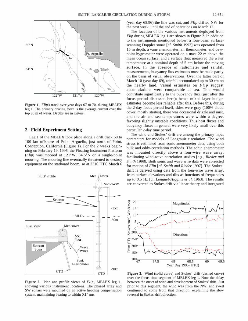
Leg 1 of the MBLEX took place along a drift track 50 to100 km offshore of Point Arguello, just north of Point.Conception, California (Figure 1). For the 2 weeks begin-ning on February 19, 1995, the Floating Instrument Platform(Flip) was moored at 121°W, 34.5°N on a single-pointmooring. The mooring line eventually threatened to destroyequipment on the starboard boom, so at 2316 UTC March 6

(year day 65.96) the line was cut, and Flip drifted NW forthe next week, until the end of operations on March 12.

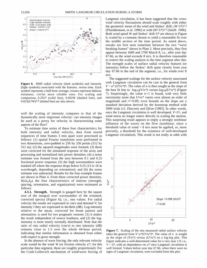
The location of the various instruments deployed fromFlip during MBLEX leg 1 are shown in Figure 2. In additionto the instruments mentioned below, a four-beam surface-scanning Doppler sonar [cf. Smith 1992] was operated from15 m depth; a vane anemometer, air thermometer, and dew-point hygrometer were operated on a mast 22 m above themean ocean surface; and a surface float measured the watertemperature at a nominal depth of 5 cm below the movingsurface. In the absence of radiometer and rainfallmeasurements, buoyancy flux estimates must be made partlyon the basis of visual observations. Over the latter part ofMarch 10 (year day 69), rainfall accumulated up to 30 cm onthe nearby land. Visual estimates on F l i p suggestaccumulations were comparable at sea. This wouldcontribute significantly to the buoyancy flux (just after thefocus period discussed here); hence mixed layer budgetestimates become less reliable after this. Before this, duringthe 2-day focus period itself, skies were gray (100% cloudcover, mostly stratus), there was occasional drizzle and mist,and the air and sea temperatures were within a degree,favoring slightly unstable conditions. Thus heat fluxes andbuoyancy fluxes in general were very likely small over thisparticular 2-day time period.

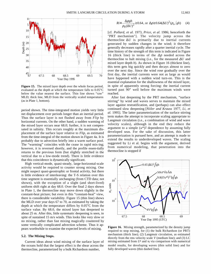
The wind and Stokes’ drift are among the primary inputparameters for models of Langmuir circulation. The windstress is estimated from sonic anemometer data, using bothbulk and eddy-correlation methods. The sonic anemometerwas mounted directly above a four-wire wave array,facilitating wind-wave correlation studies [e.g., Rieder andSmith 1998]. Both sonic and wave wire data were correctedfor motion of Flip [cf. Smith and Rieder 1997]. The Stokes’drift is derived using data from the four-wire wave array,from surface elevations and tilts as functions of frequenciesup to 0.5 Hz [cf. Longuet-Higgins et al. 1963]. The resultsare converted to Stokes drift via linear theory and integrated

120°W

35°N

122°W

34°N

Pt. Arguello

4000

30002000

1000

121°W

67

70

Figure 1. Flip 's track over year days 67 to 70, during MBLEXleg 1. The primary driving force is the average current over thetop 90 m of water. Depths are in meters.

Met. Tower

Sonic/WW

CTD

Secscan

MLD

CTD

SonicAnemometer

WaveWires

SSTFloat

SecscanSonar

Met. towerPlan View

FLIP Profile

-90m

-30m

-15m

Figure 2. Plan and profile views of Flip , MBLEX leg 1,showing various instrument locations. The phased array andSW sonars were mounted on an active heading compensationsystem, maintaining bearing to within 0.1° rms.

0

5

10

15

20

67 67.5 68 68.5 69 69.5100

150

200

250

300

Year Day 1995 (UTC)

Directions

Magnitudes

Fro

m (°

T)

Sto

kes(

cm/s

),W

ind(

m/s

)

Figure 3. Wind (solid curve) and Stokes’ drift (dashed curve)over the focus time segment of MBLEX leg 1. Note the delaybetween the onset of wind and development of Stokes’ drift. Justprior to this segment, the wind was from the NW, and swellcontinued to come from that direction, explaining the slowreversal in Stokes' drift direction.


over the directional-frequency spectrum to estimate the netdrift at the surface. On March 8 (year day 67) the wind wasinitially calm (Figure 3). It increased uniformly from the SE,beginning near 2 m/s at 0600 and reaching 12 m/s bymidnight UTC. It remained steady and strong over the nextday, finishing March 9 with a remarkably steady 15 m/sbreeze. These 2 days form the focus period for this study.The following day (year day 69) the winds became slightlymore variable, with rain squalls yielding many inches

accumulated rainfall. The wind direction also remainedsteady from the SE for the 2-day focus period, becomingslightly more variable on the following day, beginning witha brief 60° directional shift and drop to 9 m/s at about 2330UTC on March 9. Over the 2-day focus period the windstress was “well behaved,” in that discrepancies betweenbulk-formula and eddy-correlation derived values are small(with Cd = .0010 providing a good bulk estimate).

Stratification and the shear across the thermocline are

De

g.

C

10

10.5

11

11.5

12

12.5

13

13.5

14

Rescaled Temperature (45m Heatc)

Yearday 1995 (UTC)

De

pth

(m

)

67 67.5 68 68.5 69 69.5 70

0

10

20

30

40

50

60

70

De

g.

C

10

10.5

11

11.5

12

12.5

13

13.5

14

Temperature

De

pth

(m

)

0

10

20

30

40

50

60

70

Plate 1. (top) Temperature profile time series and (bottom) stretched profiles. Linear stretching of the verticalcoordinate is adjusted to make the (stretched) heat content from 0 to 45 m depth constant. This should reduce theeffect of low-mode reversible processes (e.g., internal waves or quasi-geostrophic activity).


primary input parameters to the simple “slab-type” mixedlayer models. The stratification was monitored with a rapid-profiling conductivity-temperature-depth (CTD) system,providing temperature and salinity profiles to over 400 mdepth every couple minutes. The vertical profile ofhorizontal velocity was monitored with an uplooking anddownlooking Doppler sonar system in the standard janusconfiguration, with one set of beams looking from about 90m depth up to the surface and another from there downwardseveral hundred meters. Due to sidelobe interference fromthe surface, velocity estimates within about 20 m of thesurface are unavailable from this instrument. Thus, tocomplete the shear estimate, the surface velocities estimatedfrom the PADS system (described in some detail below) areused together with velocity estimates averaged over anintermediate range interval (35-45 m) of the uplooking data.

The rapid-profiling CTD provided profiles of conductiv-ity and temperature versus depth every 1 to 4 min. Near thesurface the conductivity is unreliable due to contaminationby air bubbles. To extend the profiles as near the surface aspossible, temperature profiles are employed here (Plate 1).From data where the conductivities are valid, it was verifiedthat the temperature-density relation is tight over the focusperiod: for data in the interval 11.4° to 14°C (i.e., from 50 mdepth to the surface), the fit σT= 29.517-(0.325)T capturesover 99.7% of the variance in σT. Thus the temperature sig-nal is a good proxy for density, as well as for heat content.Internal waves can induce large isotherm displacements,especially near tidal periods. To assess this, advantage istaken of the small heat fluxes: assuming the verticalexcursions due to internal waves are primarily low mode, thevertical coordinate is scaled uniformly such that the net heatcontent from 45 m to the surface is conserved (Plate 1,bottom; note that here “small heat flux” is in comparison tothat needed to significantly change the heat content over theentire 45 m). For the purpose of this rescaling, theshallowest temperature is extended to the surface. Thisundoubtedly introduces some error near the beginning of themixing, between year days 67.2 and 67.4. In this stretchedview of the upper ocean, it appears that a mixed layer formsover the middle third of March 8 (year day 67) and thenremains nearly constant with a depth of about 25 m over thenext 2 days. The deepening occurs primarily during theincreasing wind segment, over the first quarter to halfinertial day. With the subsequent steady 15 m/s winds, the(scaled) mixed layer depth remains approximately constant.

3. PADS Data Processing

3.1. Acoustic Doppler Basics

In a Doppler sonar system, pulses of sound aretransmitted and reflect off scatterers in the medium (in thiscase, bubbles in the water). The recorded backscatter isprocessed to determine both the intensity of backscatter andthe frequency (Doppler) shift. The pulses travel outward atthe speed of sound, and knowledge of this speed is used toconvert the information into functions of range. In a typicalsystem the signal is complex demodulated such that a zeroDoppler shift would yield a zero-frequency (complex dc)signal. The temporal rate of change of phase of thisdemodulated signal yields the mean Doppler shift. Thisphase rate of change is estimated from the phase of acomplex covariance, formed between the demodulated

signal at 2 times a small time apart. The magnitude of thissame time-lagged complex covariance provides the intensityestimate. The duration of the pulses, together with the timelag used for the covariance estimates, determine the rangeresolution of the results [e.g., Rummler 1968].

The intensity (magnitude) is a good measure of bubbledensity, and the Doppler shift (phase) yields an estimate ofthe radial velocity of the cloud of scatterers. Additionalaccuracy for the phase estimates (velocity) can be obtainedwith coded pulses [Brumley et al. 1991, Smith and Pinkel1991, Pinkel and Smith 1992, Trevorrow and Farmer1992]. Here this approach is extended to an array ofreceivers, permitting simultaneous digital beam forming ofthese complex acoustic covariances, providing both intensityand Doppler shift over a continuous sector from eachtransmission. Details are described in the appendix.

For MBLEX leg 1, the PADS system was oriented so thebeam forming is horizontal, covering an area of the surface25° wide and from 190 to 450 m in range from Flip. Theintensity images shown are corrected for both attenuationand beam pattern. Values of rms velocity, etc., were found tobe insensitive to small changes in the analyzed area. Toexamine the characteristics and evolution of surface featuresover the first 40 hours of the storm, the analysis employedevery other (even) hour’s data from 0800 March 8 to 2300March 9, 1995, UTC. Over this period, the PADS axis(center-beam) heading was held near 12°T with an activecompensation system or “rotator”; this held the headingvariations to about 0.1° rms. To provide a more detailed lookat the last stages of evolution, all 10 hours from 1800 March9 to 0400 March 10 were analyzed. This final segmentincludes some especially interesting behavior (vacillations)and also includes a few hours after the wind shifts indirection, drops to 9 m/s, and then rebuilds and shifts slowlyback. It incidentally includes a PADS axis rotation to theacross wind direction (after the wind shift); this last detailprovided no surprises and so is not discussed further.

3.2. Scatterer Dynamics

The acoustic backscatter intensity fields approximatelycorrespond to horizontal maps of the vertically integratedcontent of bubbles near 15 µm radius. The Doppler shiftfields represent bubble-weighted vertically averaged radialvelocities. It is therefore worthwhile to consider briefly thegeneral behavior of the bubbles.

Conceptually, the bubbles are injected at the surface bybreaking waves and are mixed vertically by turbulence:turbulence competes against rise velocity to distribute thebubbles initially. As bubbles are mixed deeper, they arecompressed to smaller size and can dissolve (depending oneffects such as gas saturation levels, surfactants, etc.). Thecompeting effects are thought to lead to a distribution whichis roughly exponential in depth, with a 1 to 1.5 m scale[Crawford and Farmer 1987]. Significant horizontalvariability is also expected, due to both the isolated nature ofwave breaking and also to the advection into downwellingzones by larger scale motion such as Langmuir circulation[Thorpe 1982, 1986, Vagle et al. 1990, Zedel and Farmer1991, Farmer and Li 1995].

Breaking waves inject bubble clouds that dissipate slowlyover several minutes. This should result in a sudden increasein backscattered acoustic intensity at the injection point, witha more gradual decay back to the background level. Because


of strong horizontal advection by inertial currents at sea, thissignature has proven elusive in previous narrow-beam datasets from the open ocean. Only a few isolated events havebeen unambiguously identified and painstakingly handanalyzed, and these were from places where inertial currentsare small [e.g., Thorpe and Hall 1983]. Intensity informationfrom a 2-D area of the ocean surface should resolve the truetemporal evolution of the bubble plumes resulting frombreaking waves, avoiding contamination by advection acrossa narrow beam. In strong winds the breaking events becomemore common and less isolated and the bubbles might beginto act as tracers of the underlying field of Langmuircirculation. Details of the time-space distribution of bubbleclouds in stormy conditions are not yet well known, so thereis some interest in examining these distributions per se, andin tracing the evolution from the former isolated injectionevents to the latter quasi-continuous streaks.

3.3. Time Averaging and Feature Tracking

The acoustic covariance estimates were averaged over 30s segments (40 pings) in real time. With advection speedsrelative to Flip of up to 30 cm/s, this is barely short enoughto avoid significant smearing of features by the inertialadvection past Flip (up to 10 m smearing). However, it isnot long enough to reduce the surface wave orbital velocities(of the order of 1 m/s) below the size of the mixed layermotions (of the order of 3 cm/s). To attain longer averagingtimes without smearing the features, a “feature-trackingaverage” was devised, using 2-D spatial correlations of each30-s frame with the next. First, each 30-s average field ofacoustic covariances is projected by bilinear interpolationonto a 2 m by 2 m resolution, geometrically corrected, north-aligned grid, using the mean bearing of the sonar systemover each 30 s interval. The magnitudes (intensities) areused to compute 30-s-lagged spatial correlations (using 2-Dfast Fourier transforms reduces the computation time by afactor of about 100 relative to direct computation, asignificant savings for this data volume). The location of themaximum magnitude of each 30-s-lagged spatial correlationyields a two-component Lagrangian velocity estimate,discretized to 0.067 m/s. This is refined by fitting abiquadratic surface to the 5-by-5 square surrounding themaximum. The result corresponds to an area-meanhorizontal advection velocity of the bubble clouds across thefield of view, or the “feature-tracking velocity.” Theaccumulated average is shifted by the appropriate offset toalign it with the new frame (with bilinear interpolation), andthe new acoustic covariance fields are averaged in. The timeaveraging is roughly exponential, of the form

An = (1-1/T) An-1 + (1/T) Dn, (1)

with a time constant T = 3 min (or six frames), where the Aare averages and D the new data field. These geometricallycorrected, spatially overresolved, time-averaged fields ofacoustic covariance estimates are then converted to radialvelocity (in cm/s, from the phase) and 10*log10(intensity)(dB, from the magnitude) and stored for analysis and/orconstruction of movie sequences. During times of low signal(e.g., early on March 8), this feature tracking process can beunstable. In one instance, the feature tracking locked onto awave-like disturbance moving at about 60 cm/s; probably a

high-frequency internal wave packet. Once the wind roseabove 2-3 m/s, there were no more problems, and thetracking was robust.

4. Results

4.1. Feature Versus Doppler Velocities: Stokes’ Drift

The mean velocity derived from the feature-trackingalgorithm can be compared to an analogous estimate derivedfrom the Doppler (radial) velocities. The insonified areaspans about 12.5° on either side of the center direction (the“axis,” aimed toward 12°T over the focus period; e.g., seePlate 2 below). For approximately uniform flow, the along-axis component is given by a cosine-weighted mean, whichfor this geometry is essentially the area mean. The cross-axiscomponent is given by a sine-weighted mean; this roughlyamounts to taking the difference between the means overtwo much smaller areas and multiplying by 8. The along-axis component is therefore better determined. The overallagreement between the Doppler and feature-trackingvelocity is remarkable, with both velocity time seriesdescribing an inertial motion having up to 30 cm/s amplitudeover the focus time period (Figure 4a). Also shown is thevelocity jump across the thermocline, estimated bysubtracting an average over 35-45 m depth (from theuplooking sonar data) from the surface Doppler-based

-20

-10

0

10

20

30

Vel

ocity

(cm

/s)

(a) Surface Feature and Doppler Velocities

67 67.5 68 68.5 69 69.5-30

-20

-10

0

10

20

30

40

Year Day 1995 (UTC)

cm/s

(b) ∆U = UD-U35-45m

Magnitude

Figure 4. (a) Mean surface feature velocities (thick lines) versusmean Doppler velocities (thin lines) estimated from the PADSsonar data. The along-axis components (solid lines) are betterestimated than the cross-axis (dashed lines); the axis aimstoward 12°T. Note the ever-increasing difference between thetwo along-axis estimates. (b) Net velocity jump across thethermocline, estimated as the difference between the surfaceDoppler velocities and the mean from the uplooker over 35 m to45 m depth. The predominant feature in both is an inertialoscillation. Decay of the inertial shear is evident. The magnitude(thick line) of this shear dominates the mixing dynamics.


estimate. In this picture, the decay of the inertial shear isevident (Figure 4b). As we shall see, this inertial shear is thedominant source of mixing.

Note that as the sign of the flow relative to Flip reverses,the sign of the surface feature velocity minus the Dopplerestimate along-axis does not (Figure 4a, solid lines). There isa steadily increasing unidirectional difference between thetwo, which roughly parallels the increase in the wind andwaves (Figure 3). In fact, the difference-velocity in thedirection along the PADS axis matches the correspondingcomponent of Stokes’ drift at the surface (toward 12°T),calculated from the four-wire directional wave array (Figure5). The cross-axis differences are too noisy to make a similarjudgment. A unique aspect of this comparison is that theLagrangian (feature) and Eulerian (Doppler) velocities areestimated from the same signal.

The agreement between the Stokes’ drift and thedifference velocity suggests that the sonar signal arises froma depth which does not vary coherently with wave phase, sothe Doppler shift is an essentially Eulerian measurement ofradial velocity. Previously, similar sonar measurements havebeen interpreted as “semi-Lagrangian,” following thebubbles’ vertical displacements but not the horizontal [e.g.,Smith 1992]. For sound incident at a steeper incident angleon the surface, this interpretation may be valid. These previ-ous measurements were indeed made at steeper angles (from35 m depth versus 15 m here), but there is no independentevidence by which to judge the interpretation. The transitionfrom semi-Lagrangian to Eulerian behavior versus incidentangle would be a study in its own right. In any case, at lowgrazing angles, as here, the sound rays are excluded fromwave crests due to shadowing by the troughs; thus the effec-tive depth of the measurement appears to be a bubble-weighted average from the typical trough depth downward.The bubbles themselves are distributed over several meters,decaying with depth roughly like exp(-z/1.5 m) [Crawfordand Farmer 1987], yielding a centroid of measurement

about 1.5 m lower. Thus the effective measurement depth isa meter or two below the wave troughs, which arethemselves somewhat below the mean water line.

4.2. Development of Intensity Features

As noted, breaking waves inject bubble clouds thatdissipate slowly over several minutes, so the expectedsignatures are sudden increases in intensity, followed bygradual decay to the background level. In strong winds, thebreaking events are less isolated, and the bubbles becometracers of the underlying circulation. Here we attempt totrace the evolution from isolated injection events to quasi-continuous streaks.

In the early part of the wind event, after the wind hascome up but before the Langmuir circulation is too strong,intensity events suggestive of bubble injection are occa-sionally seen in the PADS data (Plate 2a). Events largeenough to be seen clearly against the background variabilityare rare: about eight events per hour exceed 6 dB above themean intensity between 1400 and 1900 UTC, March 8.Toward the latter part of this segment, streaks associatedwith Langmuir circulation also begin to show up in theintensity images. It can then be seen that the large “intensityevents” tend to occur on a preexisting streak (Plate 2b).Visually, whitecapping was common over the whole timeperiod, with every few crests spilling or breaking. Thus, onlya small fraction of breaking events produces bubble cloudswhich stand out. These could be either very large but rare“plunging breakers,” or they could be coincidental oc-currences of reasonably large breakers directly over down-welling zones in the underlying flow. The intensity eventsbecome more common as the winds and waves increase.

Streaks associated with Langmuir circulation show upshortly after the appearance of such intensity events andbecome distinct by about 0000 UTC March 9. In the earlyhours of March 9 the intensity events begin to look morelike sudden enhancements of the streak features themselves.In contrast to the earlier segment, where the intensity eventsoccur as roughly isotropic spots, the later events can beelongated, and sometimes groups of features appear to lightup simultaneously over an area several tens of meters on aside. In these cases, the features can appear in adjacentstreaks simultaneously (separated by 20 to 40 m). As notedabove, these features appear to occur along previouslyvisible streaks. Throughout this wind event, the streaks aresomewhat erratic in both time and space, in contrast to thewell-aligned features seen previously with a sudden wind“turn-on” event [Smith 1992] or in lochs or lakes. Finally,over the last even hour of March 9 (2200-2300 UTC), thefeatures “vacillate” between very distinct, intense streaksand less distinct, more erratic fields. The vacillations appearto occur simultaneously over the measurement area, with aperiod of about a half hour. This is discussed further below.

4.3. Scaling of Surface Motion

The features measured at the surface can be characterizedin terms of strength, degree of organization, spacing, andorientation. For example, Plate 3 shows four frames about15 min apart, illustrating various strengths and degrees oforganization in the flow features. One interest is to seewhether previously suggested scalings for the rms velocityhold in this new data set. A further interest is to see how

67 67.5 68 68.5 69 69.5-2

0

2

4

6

8

10

12

14

16

18

Year Day 1995 (UTC)

(Feature-Doppler) and Stokes' VelocitiesV

elo

city

(cm

/s)

Figure 5. Comparison of feature-tracking velocities minusDoppler velocities from the sector-scan sonar data (stars) versusStokes’ drift (solid line). Stokes' drift is calculated by lineartheory from directional wave-wire data. Only the along-axiscomponent is compared. For this component the netfeature–Doppler velocity difference matches the calculatedStokes’ drift.


well the scaling of intensity compares to that of thedynamically more important velocity: can intensity imagesbe used as a proxy for velocity in characterizing someaspects of the flow?

To estimate time series of these four characteristics forboth intensity and radial velocity, data from storedsequences of time frames 3 min apart were processed asfollows: (1) spatial Fourier transforms were performed intwo dimensions, zero-padded to 256 by 256 points (512 by512 m); (2) the squared magnitudes were formed; (3) thesewere corrected for the simulated response of the array andprocessing and normalized into power densities; (4) a noiseestimate was formed from the area between 0.1 and 0.25fractional power response; (5) the high wavenumbers weremasked off where the response drops below 0.25 (13 to 18 mwavelength, depending on orientation); and (6) the noiseestimate was subtracted. Results for the four example framesare shown in Plate 4. From these corrected power densities,S(t,kx,ky), the four characteristics of interest (strength,spacing, orientation, and organization) were estimated asfollows:

4.3.1. Strength. Strength is gauged here by the squareroot of the integral over wavenumber of the trimmed,corrected spectra (Figure 6); i.e., rms values. For radialvelocity the results are expressed in cm/s and denoted V; forintensity I they are expressed in decibels (dB). Log-intensityrelative to the mean, corrected for beam pattern andattenuation, is used for two pragmatic reasons: (1) it makesthe result independent of source loudness, and (2) the log-intensity is more nearly normally distributed. Note that theratio of rms radial velocity (cm/s) to rms intensity (dB)remains close to 1.5 over the whole 44-hour period,indicating that similar information is obtained from eitherwith respect to gross strength.

In the absence of wave forcing, the only relevant velocityscale would be the wind W (or friction velocity u*; for thisparticular data segment, these are roughly proportional). Forthe Craik-Leibovich mechanism of wind/wave forcing of

Langmuir circulation, it has been suggested that the cross-wind velocity fluctuations should scale roughly with eitherthe geometric mean of the wind and Stokes’ drift, (W Us)1/2

[Plueddemann, et al. 1996] or with (W2 Us)1/3 [Smith 1996].Both wind speed W and Stokes’ drift Us are shown in Figure6, scaled by a constant chosen to yield a reasonable fit overthe middle section of the time period. As noted above,streaks are first seen sometime between the two “wavebreaking frames” shown in Plate 2. More precisely, they firstappear between 1600 and 1700 March 8, i.e., after year day67.66, as the wind exceeds 8 m/s. It is therefore reasonableto restrict the scaling analysis to the time segment after this.The strength scales of surface radial velocity features (orintensity) follow the Stokes’ drift quite closely from yearday 67.66 to the end of the segment, i.e., for winds over 8m/s.

The suggested scalings for the surface velocity associatedwith Langmuir circulation can be cast in the general formV ~ u* (Us/u*)n. The value of n is then sought as the slope ofthe best fit line to log10(V/u*) versus log10(Us/u*) (Figure7). Surprisingly, the value n=1 is found, with very littleuncertainty (note that Us/u* varies over almost an order ofmagnitude and r2=0.89; error bounds on the slope are astandard deviation derived by the bootstrap method with5000 trials [cf. Diaconis and Efron [1983]. In other words,once the Langmuir circulation is well developed, V~Us, andwind stress no longer enters directly in scaling the motion.This surprising result appears to imply a strongly nonlinearinfluence of the waves on the flow (nonlinear, since athreshold value of wind > 8 m/s must be applied, or, moreprecisely, a threshold for the existence of well-developedLangmuir circulation). This result is not really at odds with

10

1

Us/u*

Slope = 0.998 ±0.037

r2=0.89

2

5

5 20

V/u

*

Figure 7. Scaling of the rms measured radial surface velocitytakes the general form V~u*(Us/u*)n. The value of n is soughtas the slope of (V/u*) versus (Us/u*) on a log-log plot. ThisFigure indicates a well-determined value for n very near 1.0; i.e.,V ~ Us, with no dependence on u* once Langmuir circulation iswell formed. Values before year day 67.66, when there were nosigns of Langmuir circulation, were excluded from this plot.

67.5 68 68.5 690

0.5

1

1.5

2

2.5

3

3.5

4

4.5

5

Year Day 1995 (UTC)

cm/s

or

dBDark Symbols=VelocityLight Symbols=IntensitySolid = 0.25 Stokes' DriftDashed = 0.2%W=1.5u*Dotted = 0.3(Usu*)1/2

Figure 6. RMS radial velocity (dark symbols) and intensity(light symbols) associated with the features, versus time. Eachsymbol represents a half-hour average; crosses represent dubiousestimates, circles more reliable ones. For scaling andcomparison, 0.25Us (solid line), 0.002W (dashed line), and0.023(UsW)1/2 (dotted line) are also shown.


the earlier reports [Plueddemann, et al. 1996, Smith 1996],as no attempt was made in these to find an optimalcombination. Rather, these works focused only on the factthat including the waves improves the fit over using thewind alone.

A comparison of the magnitude of this velocity scale isalso revealing. For SWAPP the maximum rms scale was 7cm/s with 12 m/s winds; here the rms surface velocity scaleV approaches 3.5 cm/s with 15 m/s wind, about 2.5 timessmaller as a fraction of wind speed. Alternatively, the wind-only regression from SWAPP is V = 4.4u* . For presentpurposes, u* (the friction velocity in the water) is roughlyW/750 in the SWAPP data, so this translates to V = 0.006W.In contrast, Figure 6 implies a fit toward the end of the

segment of about V = 0.0023W, or 2.6 times smaller as afraction of wind speed. The overall fit shown in Figure 6(1.5u*) is smaller than SWAPP’s by a factor of 3. InSWAPP the rms cross-wind velocity scaled better with2(u*Us)1/2 than with 4.4u* (or 0.006W) alone. Could someof the discrepancy arise from differences in the Stokes’drift? From Figure 6, the rms radial velocity toward the endscales as 0.25Us and 0.0023W (or 1.7u*). Combining theseyields 0.65(u*Us)1/2. This is different by a factor of 3.1, aneven larger discrepancy, since the ratio Us/u* is larger here(up to 6.9) than it was in SWAPP (about 4.8). Finally, it wasnoted above that the optimal fit here is between V and Us

alone. While no search for the optimal combination of Us

and u* was attempted for the SWAPP data set, this relation

Intensity dB-10 +10

1518:45 1520:15 1521:45

0 100 200

200

300

400

0 100 200 0 100 200

0 100 200

200

300

400

0 100 200

1838:15 1839:45

(a) Event 1

(b) Event 2

Meters E-W

Me

ters

N

-S

Plate 2. Intensity "injection" events. (a) Near 1520 UTC March 8 1995, before linear features are seen. There isuniform advection up to the right. Note the sudden appearance of two red spots between the first two frames, andtwo more by the next. Frames are 1.5 min apart. (b) Near 1840 March 8. Now some stripes are evident; note thatthe two spots appearing in the last frame occur over preexisting stripes. The arrows in the lower right cornersindicate the wind speed and direction. An arrow 50 m long (on the image’s scale) corresponds to a 10 m/s wind.


would imply an even larger discrepancy in the magnitudes ofV between here and SWAPP. This reduction in V could helpexplain the reduced mixing: a reduction of V by 3.1 impliesan order of magnitude less kinetic energy at the surface thanfor corresponding SWAPP-like conditions. This is addressedfurther below.

What could be responsible for this apparent reduction inthe observed velocity scale V? One possibility is the relativedirections of low-period swell relative to the wind: these

were initially opposed here and aligned in SWAPP. Thiscould directly affect the wind/wave interaction thought todrive Langmuir circulation. Another possibility is that thebubble-injection rates are unusually high for this event(perhaps also due to the existence of the opposing swell),providing some “buoyant damping” of the motion. Furtherinvestigations are needed to select between such alternativesand to determine why and when such suppression of themotion occurs.

200

250

300

350

400

03/09/95 2200:02 UTC

(±10 dB)

Distance E-W (m)0 50 100 150 200

200

250

300

350

400

Distance E-W (m)0 50 100 150 200

03/09/95 2245:02 UTC

200

250

300

350

400

200

250

300

350

400

03/09/95 2215:02 UTCD

ista

nce

N-S

from

FLI

P (

m)

Dis

tanc

e N

-S fr

om F

LIP

(m

)D

ista

nce

N-S

from

FLI

P (

m)

03/09/95 2230:02 UTC

(±20 cm/s)Intensity Velocity

Plate 3. Four frames 15 min apart during strong forcing conditions. Note how the stripes alternate between well-defined and irregular. The arrows indicate the wind; a 50 m vector (on the image’s scale) represents a 10 m/swind. North is up.


4.3.2. Spacing and orientation. To estimate bothspacing and orientation, a useful guide is the meanwavenumber. Here the wavenumber spectrum has a 180°ambiguity, and the signal is somewhat noisy. To enhance thesignal, the power densities are first squared. Then, notingthat the wind remains from the SE over this time, and thatthe orientation of the features remains fairly steady as well,the mean wavenumber is simply estimated from the upperright half of the plane (over the area where kx+ky>0; see

Plate 4):

rK(t)≡

rkS2(t,

rk )d

rk

(kx +ky>0)∫S2(t,

rk )d

rk

(kx +ky>0)∫, (2)

where S(t,k) is the spectral power density of the selectedsignal. The spacing is found from the magnitude of the meanwavenumber (Figure 8); the orientation from its angle on thewavenumber plane (Figure 9).

-50

0

50

10003/09/95 2200:02 UTC

-50

0

50

03/09/95 2215:02 UTC

-50

0

50

03/09/95 2230:02 UTC±100

0-20-30 -10

Spectral Density(dB relative to peak)

-100

-50

0

50

03/09/95 2245:02 UTC

-100 0 ±100 0 100

Intensity Velocity

±100

±100

Cyc

les/

km N

-SC

ycle

s/km

N-S

Cyc

les/

km N

-SC

ycle

s/km

N-S

Plate 4. Wavenumber spectra for the four frames of (left) intensity and (right) radial velocity shown in Plate 3.All values are relative to the maximum. The vector again represents the wind speed and direction at each time.


The maximum (and usually dominant) spacing has beenseen to track 2 to 3 times the mixed layer depth [Smith, et al.1987, Smith 1992]. Here the spacing eventually settles on 2to 2.5 times the mixed layer depth (Figure 8). In the earlyportion of the time period, the spacing is not well estimated,based on the criterion that the wavenumber uncertaintyshould be smaller than the magnitude of the mean

wavenumber estimate itself (see section 4.3.3). Unreliableestimates are marked by crosses, while the more reliableestimates are marked with open circles. The more reliableestimates occur only after the mixed layer has mixed to 20m, after which no further deepening is systematicallyobserved. Looking at only the reliable estimates, theintensity features track roughly 2 times the mixed layerdepth (MLD), while the radial velocity features tend to beslightly farther apart, at about 2.5 times the MLD. Note thatthe radial velocity features are consistently larger scale thanthe intensity.

The mean orientations of the features appear to be morerobustly estimated than the spacing. Even when the meanwavenumbers are not well determined, the orientations ofthe streaks tend to lie nearly parallel to the wind direction(i.e., the mean wavenumber lies about 90° off the wind;Figure 9a). To examine this more closely, the orientationsrelative to the wind are shown in Figure 9b. The meanorientations relative to the wind are formed over just pointswhere both radial velocity and intensity based estimates arejudged good. Surprisingly, the mean orientations of intensityversus radial velocity features are not the same: the radialvelocity features tend to lie about 10° to the right of thewind, while the intensity features average only 2° to theright of the wind.

The difference in both spacing and orientation of radialvelocity versus intensity features is a new and unexpectedobservation. This tendency is exemplified in Plate 3b: theradial velocity features have a slightly larger spacing, and anorientation slightly clockwise, relative to the features in theintensity field. This is verified by examination of the spectra(Plate 4b), which show single intense peaks at differentwavenumbers for the two fields. This shows that thedifferences in scale are not due to noise bias. Sometimes, asin Plate 4b, the peaks in intensity versus velocity spectra aredistinct and unrelated to each other; at other times there aretwo or more peaks appearing in both spectra, with onefavored by the intensity field and the other, clockwise and

67.5 68 68.5 69

0

5

10

15

20

25

30

35

40

45

50

Year Day 1995 (UTC)

Me

ters

Dark Symbols = VelocityLight = IntensityLine =Mixed Layer Depth

Figure 8. Half the feature spacing versus time (symbols), andmixed layer depth (solid line). Crosses represent dubious data.Note the velocity feature spacing (darker circles) generally liesbelow that of intensity (light circles). This relation indicates thatthe rolls are approximately as deep as they are wide.

120

140

160

180

200

220

Deg

rees

Tru

e

(a) Orientation

Dark Symbols = VelocityLight Symbols = IntensitySolid Line = Stokes' DriftDashed Line = Wind

67.5 68 68.5 69-40

-30

-20

-10

0

10

20

30

40

Year Day 1995 (UTC)

Deg

rees

Off

Mea

n (W

ind

& S

toke

s)

(b) Orientation Relative to Wind

Dark Symbols = VelocityLight Symbols = IntensitySolid Line = Stokes' Drift

Figure 9. Orientation of (a) the features relative to north, and(b) relative to the wind direction. Note that the intensity features(light symbols) consistently lie closer to the wind direction thanthe velocity features.

67.4 67.6 67.8 68 68.2 68.4 68.6 68.8 690

0.5

1

1.5

2

2.5

3

Year Day 1995 (UTC)

Dark Symbols =VelocityLight Symbols = Intensity

k/∆k

Peakiness

Figure 10. Peakiness index for intensity (light symbols) andradial velocity (dark symbols). The peakiness is also used as anindicator of quality: here, and in the related Figures, crossesrepresent cases where the peakiness falls below 7/8 (dashedline).


closer to the origin, favored by radial velocity (e.g., Plate4d). The tendency for the radial velocity features to be largerscale and further to the right of the wind than intensity isconsistent throughout the “good data” section of the timeperiod (i.e., from year day 67.66 to the end).

4.3.3. Degree of organization. One measure of thedegree of organization is the ratio of the magnitude of themean wavenumber to its uncertainty. The corresponding“peakiness” parameter (analogous to the “Q” of a dampedoscillator) is defined as

P(t)≡rK(t)

S2(t,rk )d

rk

(kx +ky>0)∫rk −

rK(t)( )2

S2(t,rk )d

rk

(kx +ky>0)∫

1/2

. (3)

Again, the squared power density is used to increase therobustness of the estimated parameters (this differentiates Pfrom the standard Q). Time series of half-hour-meanpeakiness are shown in Figure 10. The intensity I featuresgenerally have higher peakiness values than velocity V. Theratio of peakiness values Pi/Pv remains near 1.5 over thewhole time segment. For this parameter, I again appears toprovide a suitable proxy for V, at least for the longer-termaverages (but see the vacillation section, below).

Overall, peakiness increases in time, as both the wind andwaves increase in strength. However, there are a couple dipsin both peakiness series that do not correspond to variationsin the wind/wave series: one near year day 68.4 and anothernear 68.8. In particular, note that over the last 12 hours (yearday 68.5 to 69) the wind was exceptionally steady in bothmagnitude and direction, at 15 m/s from the SE, while thewaves increased only slightly in magnitude.

In addition to providing a measure of the degree oforganization or simplicity of the flow, this parameter alsoindicates when the mean vector wavenumber is reliable andis used for quality control of the spacing and orientationestimates. A simple threshold is used to distinguish between

“unreliable” (P<7/8, marked with crosses) and “morereliable” (P>7/8, marked with open circles) estimates.

4.4. Vacillations.

The example figure of four frames (Plate 3) illustratesadditional unexpected behavior. Over the course of an hour,the fields appear to vacillate between relativelydisorganized, weaker flows (Plates 3a and 3c) and moreintense, more regular features (Plates 3b and 3d). Toinvestigate this further, and in particular, to see when thevacillations begin and how long they last, a continuous 10-hour segment surrounding this hour was included in theanalysis, from 1800 UTC March 9 to 0400 March 10, 1995(day 68.75 to day 69.17). Note that the wind drops below 10m/s and briefly veers 60 degrees at about 2330 UTC March9. All features essentially disappear upon the wind changeand then build up again, paralleling the rebuilding of thewind and waves.

The vacillations appear only in these last 2 hours beforethe wind drops and veers. They show up most clearly in theintensity peakiness (Figure 11). The velocity peakiness doesnot show any convincing sign of vacillations. A discernibleresponse is also seen in the strengths of the features (Figure12): about four cycles of vacillation are seen in bothintensity and velocity strengths just before midnight UTC.Surprisingly, the strength of radial velocity is out of phasewith that of intensity: the rms intensity maxima correspondto rms velocity minima, and vice versas. The maxima in theintensity features’ strengths coincide with their peakiness, ordegree of organization. Finally, a small signal appears in thespacing data as well (Figure 13). The spacing of velocity andintensity features vary together, with slightly smaller scalescoinciding with high intensity, low velocity levels, andlarger scales coinciding with stronger velocities and weakerintensity variations. No corresponding vacillations are seenin the orientations. For these relatively quick variations,intensity is clearly not a good indicator of the flow but is acomplementary form of information.

0

1

2

3

4

5

Dark Symbols = VelocityLight Symbols = Intensity

18 20 22 24 02 04Hour UTC, Year Days 68 & 69

rms

cm/s

or d

B

Figure 12. The rms radial velocity (dark symbols) and intensity(light symbols) over the close-up segment. The vacillations areclearest between 2130 and 2330, year day 68. The velocityvariations are exactly opposite to those of intensity: maximumintensity feature strength corresponds to minimum rms velocity.

18 20 22 24 02 040

0.5

1

1.5

2

2.5

3

3.5Peakiness, 10-hour close-up

Hour UTC, Year Day 68 & 69

k/∆

k

Dark Symbols = VelocityLight Symbols = Intensity

Figure 11. Peakiness index over the 10-hour close-up period.Vacillations are prominent in the intensity peakiness (lightersymbols) but absent in the velocity peakiness (darker symbols).The wind shifts at 2330, causing the features to fade; theyrebuild slowly as the wind shifts back and picks up to 15 m/sagain.


The vacillations do not appear to be caused by variationsin the forcing. Wind and wave speeds and directions areshown in Figure 14 (scaled as before, to facilitatecomparisons with Figures 10 and 12). Correspondingvariations in the wind speed and direction are absent. Theestimated Stokes’ drift from time segments shorter than 15min are somewhat noisy; however, it is seen that thevariations are not coherent with the vacillations. Anotherpossibility is that the vacillations are forced by internalwaves. As indicated above, the mixed layer depth (MLD)over this time is a good indicator of internal wavedisplacement. As seen in Figure 13, the overall spacingroughly tracks twice the MLD, even after the wind drops andbegins to rebuild. However, over the 2 or 3 hours ofvacillations, the mixed layer oscillates with a period between1.5 and 2 hours. The vacillations in strength, spacing, andpeakiness are uncorrelated with either the MLDdisplacement or the magnitude of vertical straining.

5. Discussion

At the outset, three goals of this work were to see (1) howwell the mixed layer development is described by currentsimple modeling ideas; (2) how well previously suggestedscalings for the surface velocity variance work; and (3) towhat extent sonar intensity signals can serve as an indicatorof the flow field, and hence (with another leap of faith) ofthe underlying vorticity. As it turns out, the observationscontain, in addition, two surprises worthy of discussion. (4)There are significant vacillations, never before observed, inthe strength, spacing, and peakiness of surface featuresassociated with Langmuir circulation; and (5) the spacingand orientation of intensity (bubbles) and surface radialvelocity features do not match.

5.1. Mixing Versus Advection.

Before proceeding to the comparison with simple mixedlayer models (which are, for simplicity, one dimensional), itis worth considering the extent to which the measurementsmay be influenced by advection, both horizontal andvertical.

First, consider uniform uplift of the deeper isotherms,with horizontal spreading or advection of the surface layer(this could be accomplished by upwelling or quasi-geostrophic activity, for example). This would result in netcooling over a fixed depth interval near the surface, say from0 to 45 m depth. To examine this possibility, the depth axiswas rescaled by a constant for each time step such that theheat content in the top 45 m remains constant (Plate 1b). Theraw and rescaled MLD are both shown in Figure 15. As afringe benefit, this rescaling appears somewhat successful inremoving distortions due to higher frequency internal waves;however, the halt in mixed layer deepening is made evenmore clear. Indeed, low-mode straining appears to beincreasing the mixed layer depth in time, consistent with thefact that the platform is drifting with the flow into deeperwater. Low-mode vertical straining or uplift can be ruled outas an explanation for halted deepening.

Next, consider horizontal advection. Flip was freelydrifting over this period, moving with the mean over theupper 90 m of the flow plus a small contribution due towindage. The surface layer exhibits inertial motion relativeto Flip (see Figure 4): the surface motion reverses in time,with about 1.5 inertial periods represented in the 1.5-day

18 20 22 24 02 04

120

140

160

180

200

Hour UTC, Year Days 68 & 69

Direction:Solid Line = Stokes' DriftDashed Line = Wind

0

1

2

3

4

cm/s

Scaled speeds:Solid Line = 0.25*Stokes' DriftDashed Line = 0.2% Wind

°T

(a)

(b)

Figure 14. (a) Scaled wind speed W (dashed line) and Stokes'drift Us (solid line) and (b) their directions. No "vacillations" inwind speed or direction are seen. Careful comparison of thenoisier Stokes' drift estimate shows that the variability is notcorrelated with the vacillations in the intensity and radialvelocity features.

18 20 22 24 02 04

0

10

20

30

40

50

Hour UTC, Year Days 68 & 69

Met

ers

Dark Symbols = VelocityLight Symbols = IntensityDashed Line = Mixed Layer Depth

Figure 13. Half the spacing (connected symbols) and mixedlayer depth (dashed line). During the vacillations (2130 to 2330),the spacing of features in both intensity and radial velocityoscillates together, with minimum spacing coinciding withmaximum intensities, minimum velocities (compare with Figure12). After the wind drops, just before 0000 day 69, the mixedlayer shoals. Plate 1 indicates this is partly accounted for by low-mode "vertical stretching."


period shown. The time-integrated motion yields very littlenet displacement over periods longer than an inertial period.Thus the surface layer is not flushed away from Flip byhorizontal currents. On the other hand, a sudden warming ofthe mixed layer occurs near 68.0; further, it is not compen-sated in salinity. This occurs roughly at the maximum dis-placement of the surface layer relative to Flip, as estimatedfrom the time-integral of the motion shown in Figure 4a. It isprobably due to advection briefly into a warm surface pool.The “warming” coincides with the cease in rapid mix-ing;however, it is reversed shortly, and the profile essen-tiallyreturns to the previous form (but slightly stretched in thevertical due to a low-mode trend). There is little evidencethat this coincidence is dynamically significant.

High vertical-mode, quasi-steady, large-horizontal-scaleactivity would be required to counter strong mixing. Onemight suspect quasi-geostrophic or frontal activity, but thereis little evidence of interleaving: the T-S relation over thistime segment is essentially unchanging (from CTD data; notshown), with the exception of a slight (and short-lived)uniform shift right at day 68.0. Over the final 2 days shownin Plate 1, the thermocline may move down slightly in theconstant-heat picture; but even in this “constant-heat” view,there is considerable variability. Figure 15 (thin line) showsthe MLD over year days 67 to 70, as estimated by taking thedepth at which the temperature differs by 0.05°C from thesurface value. By 68.0, the mixed layer has deepened toabout 25 m. After this, little systematic deepening is seen, inspite of sustained 15 m/s winds. This looks like very slow orno mixing, rather than fast mixing magically countered bysome vertically complicated advection scheme. Thus it ap-pears worthwhile to examine the expected levels of mixing.

5.2. The Mixing Stops.

Current ideas about wind mixing of the surface layer ofthe oceans hold that the largest effect is the shear across thethermocline, parameterized by a bulk Richardson number,

Ri≡ ∆ρgh

ρ0(∆U)2 ≥0.64, or ∆ρ≥0.64(∆U)2(ρo gh) (4)

[cf. Pollard, et al. 1973, Price, et al. 1986; henceforth the"PRT mechanism"]. The velocity jump across thethermocline ∆U is primarily due to inertial currentsgenerated by sudden changes in the wind; it thereforegenerally decreases rapidly after a quarter inertial cycle. Thetime history of the strength of this term is indicated in Figure16 (thick line) in terms of the ∆ρ needed across thethermocline to halt mixing (i.e., for the measured ∆U andmixed layer depth h). As shown in Figure 16 (thickest line),this term gets big quickly and then decays almost to zeroover the next day. Since the wind rose gradually over thefirst day, the inertial currents were not as large as wouldhave happened with a sudden wind turn-on. This is theessential explanation for the shallowness of the mixed layer,in spite of apparently strong forcing: the inertial currentturned past 90° well before the maximum winds werereached.

After fast deepening by the PRT mechanism, “surfacestirring” by wind and waves serves to maintain the mixedlayer against restratification, and (perhaps) can also effectcontinued slow deepening [Niiler and Krauss 1977, Li, etal. 1995]. The latter parameterization of the surface stirringterm makes the attempt to incorporate scaling appropriate toLangmuir circulation (i.e., a combination of wind and wavevelocity scales), although in the end they reduce theargument to a simple (u*) 2 dependence by assuming fullydeveloped seas. For the sake of discussion, this latterparameterization is pursued here, and an attempt is made toextend the results to underdeveloped waves. The scalingsuggested by Li et al. begins with the argument, derivedfrom numerical modeling, that penetration into thethermocline is stopped if

67 67.5 68 68.5 69 69.5 70

5

10

15

20

25

30

35

40

45

0

Year Day 1995

Dep

th (

m)

Figure 15. The mixed layer depth over the whole focus period,evaluated as the depth at which the temperature falls to 0.05°Cbelow the value nearest the surface. Thin line shows “raw”MLD; thick line, MLD from the vertically scaled temperatures(as in Plate 1, bottom).

67.5 68 68.5 69

10-2

10-1

100

Year Day 1995 (UTC)

σ T u

nits

0.65 |∆U|2/gh

50(u*)2ρ/gh

9.8(Usu*2)2/3ρ/gh

4V2ρ/gh

Figure 16. Mixing strength, parameterized by the density jumprequired to stop mixing, for (1) the bulk Richardson (or PRT)mechanism (thick line); (2) Langmuir circulation, as estimateddirectly from the rms velocity scale V (medium line); and (3) LCmixing estimated from Us and νt via comparison with numericalmodel results, for developing waves (thin solid line) and forfully developed waves (thin dashed line).


∆ρ≥1.23wdn2 (ρo gh), (5)

where wdn is the maximum downwelling velocity associatedwith the Langmuir circulation. Using model results for wdn,they rewrite this in the form

∆ρ≥Cu*2 (ρo gh) (6)

where

C≡0.36Us kνt , (7)

in which νt is the turbulent kinematic eddy viscosity and k isthe wavenumber of the dominant surface waves. For fullydeveloped seas, they argue C is about 50 (Figure 16, thindashed line). This criterion is evaluated two ways here: (1)using the rms horizontal scale to estimate wdn directly foruse in (5), or (2) extending the evaluation of C to under-developed waves, using estimates of Us, k, and νt in (7).

Since the spacing is about twice the mixed layer depth,the rolls appear to be roughly isotropic in the cross-windplane. It is therefore reasonable to assume the vertical andcross-wind velocity scales are comparable. Assume also thatthe rms radial velocity scale V derived from the PADSmeasurements is a good estimate of the cross-windcomponent size. Finally, to estimate the maximumdownwelling velocity from an rms, an argument analogousto that for significant wave height from rms displacement isneeded. In brief, the circulation is not simply sinusoidal (inwhich case wmax ~ 21/2V) but varies somewhat randomly. Asin the case of wave height, we need to set a threshold, say,one exceeded by 1/3 of all downwelling local maxima. Thisleads to a value roughly 2 times the rms. Hence wesubstitute 4V2 from the PADS measurements (section 4.3.1)for wdn in (5). This provides a fairly direct estimate of thestrength of mixing due to the observed Langmuir cells(Figure 16, medium width line).

For the indirect approach, a significant requirement isestimation of νt. Recent dissipation measurements near thesurface indicate that the turbulent velocity scale q isreasonable well described by the energy dissipation rate ofthe waves [e.g., Terray et al. 1996]. This, in turn, is wellestimated by the energy input to the waves (within 7% orso). The growth rate β of a wave of radian frequency σ andphase speed c is approximately β = 33σ (u * /c)2 [Plant1982], so the net energy flux can be written in the form

q3 ∝ ρ−1βE = 33ga2σ (u * /c)2 = 33(Usu *2 ). (8)

Conveniently, the final form in (8) remains approximatelyunchanged with integration over the wave spectrum (withperhaps a factor representing the typical directional spread).The length scale appropriate to wave breaking isproportional to the wave amplitude a, so we obtain anestimate of νt of the formνt ∝ a(Usu *2 )

13 . Substituting this

into (7), and noting that ak in general does not varysignificantly from about 0.1, we obtain

C∝Us kνt ∝(Us u*)2/3 (9)

The values employed by Li et al. for fully developed wavesimply Us/u* → 11.5. To obtain 50 with this value in (9), theconstant of proportionality is set to 9.8. Then (6) becomes

∆ρ≥9.8(Us u*2 )2/3(ρo gh). (10)

This criterion is also shown in Figure 16 (thin solid line).It is seen that the mixing effect estimated from the

measured velocities falls far below the parametric estimate(10). The discrepancy is very similar in magnitude to thatbetween the velocity scale observed here versus SWAPP:the velocity variance V2 measured here (and hence thecorresponding mixing effect) is smaller by a factor between6 and 10 (thus the SWAPP variance estimates wouldpresumably agree closely with (10)). Over a period ofseveral days, such a reduction could lead to a significantdifference in the mixed layer depth. It is therefore importantto understand why this variance is reduced. Again, it isconjectured that the existence of opposing swell isimportant, either directly via the wave/current generationmechanism of Langmuir circulation or indirectly viaenhanced wave breaking and bubble injection.

5.3. Vacillations

Vacillations have been described in some simulations ofLangmuir circulation [e.g., Tandon and Leibovich 1995,henceforth TL95]. For strong forcing conditions (definedbelow), TL95 find instabilities with two timescales: one“slow” oscillation in strength and organization and a “fast”variation associated with propagation of sinuousperturbations downwind. The slow oscillation has maximumdistortions at the times of strongest rms cross-windvelocities and minimum distortion in between. Thiscompares favorably with the maximum intensity peakinessbeing observed to coincide with the minimum rmsvelocities. However, the timescale of the simulatedoscillations corresponds here to tens of hours. At periods oftens of minutes, the fast oscillations might appear attractivefor comparison; however, these are self-similar formspropagating downwind and would show up as such in the 2-D views presented here.

The equations used in TL95 depend on two parameters.One is a Reynolds number, Re=u*d/νt, where d is the mixedlayer depth and νt is the eddy viscosity, assumed constant.The other is a Rayleigh number, which can be written in theform R=Re3(Us/u*). For initial (2-D) instabilities, only Renters, and the critical number for the onset of Langmuircirculation is about Rc=669 (presumably depending ondetails of the geometry and boundary conditions).

The eddy viscosity, and hence Re, is hard to estimate(notwithstanding the arguments of section 5.2). On the otherhand, it is straightforward to compute Us/u* (Figure 17).One approach is to assume that the “turbulence” (all motionexcluding the Langmuir circulation (LC)) adjusts so that Reremains constant. Then let R=Rc at the moment LCs are firstdetected, i.e., no sooner than year day 67.66 (as notedabove). At that time, Us/u* is about 2 and increasing rapidly(Figure 17); thus Re=(669/2)1/3=6.9. For Re=5.9, TL95 findno oscillatory instabilities no matter how much R isincreased. The oscillatory behavior is observed for R>900and Re=22.36 (or Re3=11,180), but this large a value for Reis hard to reconcile with the observed onset of LC activity.To get R below the critical value would require Us/u*<0.06.The lower bound on Re for such oscillatory instabilities hasnot been established. Given both this and the mismatch intimescales, comparison with the simulations is notconvincing. Furthermore, if we use the viscosity estimate ofsection 5.2, Re actually decreases between the onset of LC


and the vacillations. Indeed, it would appear possible that theparameters are moved back to marginal stability rather thanto “overforced” conditions.

An interesting possibility is that the bubbles influence thedynamics. For 15 m/s winds the volume fraction of bubblesa meter below the surface is expected to be about 10-6 [e.g.,Crawford and Farmer 1987]. During the intense phase ofthe vacillations, the intensity varies by ±10 dB, yieldingestimated volume fractions of 10-5 at the convergences. Thiscorresponds to a density anomaly of 0.01 kg/m3, yielding areduced gravity acceleration of 10-4 m/s2. This accelerationwould stop a downwelling velocity of 6 cm/s in 10 min. Thebubbles do not disappear instantly, so the flow couldactually reverse due to continued buoyancy forcing, or thestructures could simply break up and dissipate. If the flowreverses, the reversed flow could be reinforced by the sameLC instability mechanism (e.g., the freshly upwelled water isnow moving downwind more slowly, inducing a wave forcereinforcing the upwelling). This would produce newintensity maxima falling somewhere between the maxima ofthe previous cycle (over the half-hour between maxima,advection moves the features beyond the sample area, so thispossibility can not be directly tested). Alternatively, thestructures could simply regenerate from scratch. In theformer scenario the rolls would oscillate back and forth,with upwelling and downwelling zones exchanging places at

each half cycle; in the latter the locations from onerealization to the next would be random. In either case, rmsvelocity maxima would occur halfway between the intensitymaxima in time, as observed. To pursue the first possibility abit, in this case the intensity maxima occur every half cycle,so the period of oscillation is an hour. A sinusoidaloscillation having an hour period with velocity maxima of 6cm/s would produce displacements of ±35 m. Over this timesegment, the rolls have about 25 m spacing, so this isenough displacement to move bubbles back and forth intothe downwelling zones (and some distance downward).Accelerations associated with such oscillating rolls wouldreach 0.0001 m/s2, about equal to the estimated reducedgravity value. Thus buoyancy forcing by bubbles produces aself-consistent scenario, demonstrating that it is feasible forbubble buoyancy to be important to the overall forcing.Similar arguments apply for the regeneration case: theestimated displacements are sufficient to sweep the surfacebubble clouds into the downwelling lines and “shut off” thecirculation; these must then regenerate in 15 min or so(consistent with typical LC growth rates) before the bubblesare again sufficiently well organized to stop the flow.

In either scenario, the occurrence of vacillations is linkedto a high level of bubble generation; thus it would beappropriate to parameterize it in terms of some measure ofwave breaking. A reasonable conjecture is that bubbledensity is related to the rate of wave breaking. A reasonableapproach is to combine the arguments of section 5.2 with thearguments of Bagnold [1962] for self-suspending turbiditycurrents (that the turbulent velocity scale q must exceed thesettling velocity, but here with the buoyancy and verticalaxes reversed). Then the maximum bubble size, and hencetotal bubble density (assuming a self-similar spectrum ofbubbles), is parameterized by q ~ (Usu*2)1/3 (Figure 17b).The vacillations only occur only over the 2 hours where thisparameter exceeds 3.6 cm/s. Such a wind-wave parameterindicative of wave breaking has proven elusive to verify;however, visual observations during this segment confirmthat wave breaking was vigorous. Interestingly, this particu-lar combination (Usu*2)1/3 also can parameterize the theoret-ical strength of forcing of the Langmuir circulation: in otherwords, from a scaling point of view, turbulence, bubbledensity, and Langmuir cell forcing may be indistinguishable.

5.4. Relations Between I and V

In terms of overall strength and organization (e.g., hourlymeans), the statistics of I (intensity) correlate well with thoseof V (radial velocity). However, in terms of the orientationand spacing, there is a surprising but consistent difference:the intensity features tend to be slightly smaller in scale (2.0versus 2.5 times the mixed layer depth) and more nearlyaligned with the wind (2° versus 10°). Further, this is notsimply a matter of different weightings of broaddistributions. For example, in Plate 4b, unimodal peaksappear in the spatial spectra of I and V but in differentlocations. In detailed comparisons (e.g., section 4.4, duringthe vacillations), even the strength and organization valuescan differ, with half-hour period variations occurring out ofphase between I and V. These puzzling differences betweenthe distribution and behavior of I versus V do not appear tohave a simple explanation.

The link between spatial distributions of the bubbles(intensity) and the velocity field has not been rigorously

0

1

2

3

4

5

6

7(a) (Us u*)/u*2

67.5 68 68.5 690

0.5

1

1.5

2

2.5

3

3.5(b) (Us u*2)1/3

Year Day 1995 (UTC)

cm/s

Ra

tio

Figure 17. (a) Ratio of Stokes' drift to friction velocity, Us/u*.The ratio is formed with a vector dot-product, so that opposingwind and waves produce a negative ratio as seen early on yearday 67. The ratio increases over the course of the storm, finallyskyrocketing when the wind relaxes, and staying high until thewind resumes. (b) Scaling arguments lead to the idea that bubbledensity, viscosity, and Langmuir circulation strength each mayscale with q = (Usu*2)1/3. In particular, note the brief butdistinct peak in this parameter near the end of year day 68.Vacillations are seen only over the time of this peak (for q>3.6cm/s).


investigated. Given that the velocity fields vary in time andthat bubble dynamics involve wave breaking, surfactants,gas saturation levels, and pressure effects (to name a few), itis plausible that bubble distributions are not always reliableindicators of the instantaneous flow. The bubble field is acomplex time integral of both the velocity field and somenonnegligible (and marginally understood) chemistry. Thus,given the observed mismatches, caution is advised in usingintensity maps as indicators of surface convergence zones,much less as indicators of the underlying vorticity.Simulations of the behavior of bubble clouds may help tounderstand these differences. In situ correlations between(for example) vertical velocity and bubble density may alsohelp. This is suggested as a reasonable avenue of research.

6. Conclusions

1. The mixed layer deepened rapidly initially, to about 20m. After the inertial current veered more than 90° off thewind, the mixing slowed. This is consistent with currentthinking, where the “bulk dynamics” of shear across thethermocline due to inertial motion is the primary agent fordeepening. Surface stirring by the combined action of windand waves may have helped maintain the mixed layer afterthis and may even have induced some additional slowdeepening. In any case, it is emphasized that the inertialcurrent “bulk Richardson number” mechanism is the lowestorder term in wind-induced mixing (and no model iscomplete without it).

2. The magnitude of surface velocity variance associatedwith the mixed layer motion, as observed here, isconsiderably smaller than in previously reported cases. It issuggested that this is related to swell opposing the wind.

3. For the data considered here, rms velocities associatedwith the low-frequency features scale quite tightly with theStokes’ drift alone, rather than with the wind or acombination of wind and waves. This relation is nonlinear inthe sense that a threshold must be set for the existence ofLangmuir circulation before it holds.

4. Langmuir circulation can vary significantly in strength,spacing, and peakiness over timescales of the order of 15min. Neither the wind, waves, nor mixed layer depths varysignificantly on this timescale. In these “vacillations,” thestrengths of velocity versus intensity features were 180° outof phase: strongest intensity features coincided with weakestrms velocities. It is suggested that the buoyancy of bubblesmay be nonnegligible in the dynamics of these phenomena.

5. Overall strength and peakiness values correlate wellbetween intensity and velocity features (over timescalescomparable to a day). However, in details such as spacing,orientation, or short-time behavior, significant differencescan occur. Also, the typical spacing and orientation ofintensity versus velocity features near the surface differ. Forthe data studied here, intensity features aligned within acouple degrees of the wind (favoring the right), while thevelocity features were typically 10° to the right of the wind.The intensity spacing tracks 2 times the mixed layer depth,while the velocity feature spacing is closer to 2.5 timesMLD. While this mismatch is puzzling, it would appearlikely that the time/space-dependent behavior of bubbles in atime-varying flow should be investigated. Simulations withrealistic bubble dynamics may help to understand thesedifferences.

6. The difference between mean feature-tracking andDoppler velocity estimates provides a reasonable and directestimate of the Stokes’ drift near the surface. A uniqueaspect is that both estimates come from the same datastream, without explicitly resolving the waves.

Appendix

The PADS system operates by transmitting repeat-sequence codes [Pinkel and Smith 1992] over a 25°(horizontal) by 2° (vertical) swath, and receiving on ahorizontal array of 16 receivers. The receivers are arrangedin a semisparse array of the form “1111-1111-0000-0000-1111-0000-1111,” where the 1’s represent receivers and the0’s represent gaps of a size equal to a receiver (the dashesare to make this easier to read; they represent no space). Thespacing is as uniform as practical, at 0.976 cm per unit onaverage. This configuration provides four or more pairs ateach spatial lag up to 24, tapering to one pair at themaximum separation of 27 units (center to center). This“semisparseness” trades some phase uncertainty (velocityerror) for added angular resolution, relative to a simple 16-in-a-row array. For sound at 194.3 kHz, 12°C, salinity 33,and 16 m depth (typical of conditions here), the Nyquistwavenumber of the receiver array corresponds to 23.2° off-axis. The 194.3 kHz center-frequency signal from eachreceiver is electronically mixed to a nonzero frequency anddigitized with 16 bit accuracy. The mix frequency is selectedto produce four samples/cycle at the center frequency withno Doppler shift. To avoid aliasing of the signal across zerofrequency with this one-sided mixing scheme, we initiallyoversample by a factor of 2; thus the repeat-sequence code“bits” are four samples long, and the signal is constrained tothe center half of the sampling bandwidth. The amplifiers,mixing, and filtering electronics maintain nearly the full 96dB dynamic range achievable with 16 bit digitization. Thisobviates the complexity and uncertainties associated with atime-variable gain, as the signal varies about 70 dB fromnear to far range. The digitized signal is computationallyremixed and filtered to a complex signal having zerofrequency for zero Doppler shift and resampled to 0.25 timesas many complex points (C samples).

Matrices of time-lagged covariances are then formed as afunction of range: the signal at one C sample on a givenreceiver is multiplied by the conjugate of each signal at theprevious C sample, resulting in a set of 16 by 16 matrices ofcovariances versus range. Because of the finite time lag,these matrices are not symmetric except in the case ofexactly zero Doppler shift. The matrices of covariances areaveraged over a specified range interval (2.7 m) and furtheraveraged over consecutive pings (keeping range binsaligned) for a specified time interval (40 pings or 30 s).Retaining the full set of matrices for each range permitspostcalibration of the receivers and refinement of beam-forming strategies. The penalty is 256/55, or about 5 timeslarger, storage requirements relative to storing onlynonredundant lags.

The following postcalibration scheme was adopted aseffective and robust: for each hour, the full hour time-averaged covariance matrix is formed for each range. Thematrix’s column averages represent the covariances of eachindexed receiver with the mean signal. These provide anempirical amplitude and phase relative to the mean of all


receivers. This can be range dependent, as the angle ofincidence varies with range, and the receivers do not haveidentical beam patterns in the vertical. To facilitate display, alog-linear profile (corresponding to constant attenuation) isfit to the hour-mean intensities over a central range intervaland compensated for. The hour averages do not vary muchfrom hour to hour but can change over the course of a day,especially as wind and wave conditions change. Thecalibrated, attenuation-corrected covariances are finallyaveraged into a nonredundant array, windowed with aKaiser-Bessel fifth order window, zero-padded to 128points, and fast Fourier transformed. The FFT outputcorresponds to beams at an array of 128 angles from -23.2 to+23.2° off axis. This array wraps around at ±23.2°; to avoidconfusion, the transmitted beam pattern was designed toinsonify only the central ±12.5°, and the outer 10.7° on eachside is discarded. The combined transmit-receive beampattern is computed from the hour-average covariances, andthe retained 25° wedge is corrected for this in the intensityplots shown.

Acknowledgments. Thanks are due to the many people involvedin MBLEX for making it a success. Regarding the gathering of thisparticular data, thanks go especially to Eric Slater, Lloyd Green, MikeGolden, Chris Neely, R. Pinkel, K. Rieder, M. Alford, and to the crewof the research platform Flip, captained by Tom Golfinas. Thanks alsofor useful comments from R. Pinkel, C. Garrett, A. Tandon, and W.Drennan concerning this work and interpretation. This work wassupported by the Office of Naval Research, grants N00014-93-1-0359and N00014-96-1-0030.

References

Bagnold, R. A., Autosuspension of transported sediment: Turbiditycurrents, Proc. R. Soc. London, Ser. A, 265, 315, 1962.

Brumley, B. H., R. G. Cabrera, K. L. Deines, and E. A. Terray,Performance of a broad-band acoustic Doppler current profiler,IEEE J. Oceanic Eng., 16, 402-407, 1991.

Cox, S. M., and S. Leibovich, Langmuir circulations in a surface layerbounded by a strong thermocline, J. Phys. Oceanogr., 23, 1330-1345, 1993.

Cox, S. M., and S. Leibovich, Large-scale Langmuir circulation anddouble-diffusive convection - evolution equations and flowtransitions, J. Fluid Mech., 276, 189-210, 1994.

Cox, S. M., S. Leibovich, I. M. Moroz, and A. Tandon, Nonlineardynamics in Langmuir circulations with O(2) symmetry, J. FluidMech., 241, 669-704, 1992.

Craik, A. D. D., The generation of Langmuir circulation by aninstability mechanism, J. Fluid Mech., 81, 209-223, 1977.

Craik, A. D. D., and S. Leibovich, A rational model for Langmuircirculations, J. Fluid Mech., 73, 401-426, 1976.

Crawford, C. B., and D. M. Farmer, On the spatial distribution ofocean bubbles, J. Geophys. Res., 92, 8231-8243, 1987.

Diaconis, and B. Efron, Computer-intensive methods in statistics, Sci.Am., 248, 116-130, 1983.

Farmer, D., and M. Li, Patterns of bubble clouds organized byLangmuir circulation, J. Phys. Oceanogr., 25, 1426-1440, 1995.

Garrett, C., Generation of Langmuir circulations by surface waves– Afeedback mechanism, J. Mar. Res., 34, 117-130, 1976.

Langmuir, I., Surface motion of water induced by wind, Science, 87,119-123, 1938.

Leibovich, S., Convective instability of stably stratified water in theocean, J. Fluid Mech., 82, 561-581, 1977.

Leibovich, S., On wave-current interaction theories of Langmuircirculations, J. Fluid Mech., 99, 715-724, 1980.

Leibovich, S., The form and dynamics of Langmuir circulations,Annu. Rev. Fluid Mech., 15, 391-427, 1983.

Leibovich, S., and S. Paolucci, The Langmuir circulation as a mixingmechanism in the upper ocean, J. Phys. Oceanogr., 10, 186-207,1980.

Leibovich, S., and A. Tandon, Three-dimensional Langmuir

circulation instability in a stratified layer, J. Geophys. Res., 98,16,501-16,507, 1993.

Li, M., and C. Garrett, Mixed layer deepening due to Langmuircirculation, J. Phys. Oceanogr., 27, 121-132, 1997.

Li, M., K. Zahariev, and C. Garrett, Role of Langmuir circulation inthe deepening of the ocean surface mixed layer, Science, 270,1955-1957, 1995.

Longuet-Higgins, M. S., D. E. Cartwright, and N. D. Smith,Observations of the directional spectrum of sea waves using themotions of a floating buoy, in Ocean Wave Spectra: Proceedingsof a Conference, Edited by National Academy of Sciences, pp.111-132, Prentice-Hall, Englewood Cliffs, N.J., 1963.

McWilliams, J., P. P. Sullivan, and C.-H. Moeng, Langmuirturbulence in the ocean, (preprint), 1997.

Niiler, P. P., and E. B. Krauss, One-dimensional models of the upperocean, in Modeling and Prediction of the Upper Layers of theOcean, Edited by E. B. Krauss, pp. 143-172, Pergammon,Tarrytown, N. Y., 1977.

O'Brien, M. M., A. Plueddemann, and R. A. Weller, The response ofoceanic mixed layer depth to physical forcing - modelled vsobserved, Biol. Bull., 181, 360-361, 1991.

Pinkel, R., and J. A. Smith, Repeat-sequence coding for improvedprecision of Doppler sonar and sodar, J. Atmos. Oceanic Technol.,9, 149-163, 1992.

Plant, W. J., A relationship between wind stress and wave slope, J.Geophys. Res., 87, 1961-1967, 1982.

Plueddemann, A. J., J. A. Smith, D. M. Farmer, R. A. Weller, W. R.Crawford, R. Pinkel, S. Vagle, and A. Gnanadesikan, Structure andvariability of Langmuir circulation during the surface wavesprocesses program, J. Geophys. Res., 101, 3525-3543, 1996.

Pollard, R. T., P. B. Rhines, and R. Thompson, The deepening of thewind-mixed layer, Geophys. Fluid Dyn., 4, 381-404, 1973.

Price, J. F., R. A. Weller, and R. Pinkel, Diurnal cycling:Observations and models of the upper ocean response to diurnalheating, cooling, and wind mixing, J. Geophys. Res., 91, 8411-8427, 1986.

Rieder, K. F., and J. A. Smith, Removing wave effects from the windstress vector, J. Geophys. Res., 103, 1363-1374, 1998.

Rummler, W. D., Introduction of a new estimator for velocity spectralparameters. (Rep. MM-68-4141-5), AT&T Bell Labs., MurrayHill, N.J., 1968

Skyllingstad, E. D., and D. W. Denbo, An ocean large-eddysimulation of Langmuir circulations and convection in the surfacemixed layer, J. Geophys. Res., 100, 8501-8522, 1995.

Smith, J. A., Observed growth of Langmuir circulation, J. Geophys.Res., 97, 5651-5664, 1992.

Smith, J. A., Observations of Langmuir circulation, waves, and themixed layer, in The Air Sea Interface: Radio and Acoustic Sensing,Turbulence, and Wave Dynamics, Edited by M. A. Donelan, W. H.Hui, and W. J. Plant, pp. 613-622, Univ. of Toronto Press,Toronto, Ont., 1996.

Smith, J. A., and R. Pinkel, Improvement of Doppler estimationthrough repeat sequence coding, in Oceans '91/Proceedings,October 1-3, 1991, Honolulu, Hawaii, USA/Ocean Technologiesand Opportunities in the Pacific for the 90's, Edited by pp. 977-984, IEEE, Piscataway, N.J., 1991.

Smith, J. A., R. Pinkel, and R. Weller, Velocity structure in the mixedlayer during MILDEX, J. Phys. Oceanogr., 17, 425-439, 1987.

Smith, J. A., and K. F. Rieder, Wave induced motion of FLIP, OceanEng., 24, 95-110, 1997.

Tandon, A., and S. Leibovich, Simulations of three-dimensionalLangmuir circulation in water of constant density, J. Geophys.Res., 100, 22613-22623, 1995.

Terray, E. A., M. A. Donelan, Y. C. Agrawal, W. M. Drennan, K. K.Kahma, A. J. Williams, P. A. Hwang, and S. A. Kitaigorodskii,Estimates Of Kinetic Energy Dissipation Under Breaking Waves,Journal Of Physical Oceanography, 26, 792-807, 1996.

Thorpe, S. A., On the clouds of bubbles formed by breaking windwaves in deep water, and their role in air-sea gas transfer., Philos.Trans. R. Soc. London, Ser. A, 304, 155-210, 1982.

Thorpe, S. A., Bubble clouds: A review of their detection by sonar, ofrelated models, and of how Kv may be determined., in OceanicWhitecaps and Their Role in Air-Sea Exchange Processes, Editedby E. C. Monahan and G. Mac Noicall, pp. 57-68, D. Reidel,Norwell, Mass., 1986.

Thorpe, S. A., The breakup of Langmuir circulation and the instabilityof an array of vortices, J. Phys. Oceanogr., 22, 350-360, 1992.


Thorpe, S., and A. J. Hall, The characteristics of breaking waves,bubble clouds, and near-surface currents observed using side-scansonar, Cont. Shelf Res., 1, 353-384, 1983.

Trevorrow, M. V., and D. M. Farmer, The use of Barker codes inDoppler sonar measurements, J. Atmos. Oceanic Technol., 9, 699-704, 1992.

Vagle, S., W. G. Large, and D. M. Farmer, An evaluation of theWOTAN technique of inferring oceanic winds from underwaterambient sound, J. Atmos. Oceanic Technol., 7, 576-595, 1990.

Weller, R., J. P. Dean, J. Marra, J. Price, E. A. Francis, and D. C.Boardman, Three-dimensional flow in the upper ocean, Science,227, 1552-1556, 1985.

Zedel, L., and D. Farmer, Organized structures in subsurface bubbleclouds - Langmuir circulation in the open ocean, J. Geophys. Res.,96, 8889-8900, 1991.

J. A. Smith, Scripps Institution of Oceanography, code 0213, La

Jolla, CA 92093-0213. (e-mail: [email protected])

(Received May 7, 1997; revised November 12, 1997;accepted December 1, 1997.)

evolution of langmuir circulation during a storm - jerry...

Documents