evolution of a location-based online social network: analysis …cm542/papers/imc2012.pdf ·...
TRANSCRIPT

Evolution of a Location-based Online Social Network:Analysis and Models
Miltiadis AllamanisComputer Laboratory
University of [email protected]
Salvatore ScellatoComputer Laboratory
University of [email protected]
Cecilia MascoloComputer Laboratory
University of [email protected]
ABSTRACTConnections established by users of online social networksare influenced by mechanisms such as preferential attach-ment and triadic closure. Yet, recent research has foundthat geographic factors also constrain users: spatial prox-imity fosters the creation of online social ties. While theeffect of space might need to be incorporated to these socialmechanisms, it is not clear to which extent this is true andin which way this is best achieved.
To address these questions, we present a measurementstudy of the temporal evolution of an online location-basedsocial network. We have collected longitudinal traces over 4months, including information about when social links arecreated and which places are visited by users, as revealedby their mobile check-ins. Thanks to this fine-grained tem-poral information, we test and compare whether differentprobabilistic models can explain the observed data adoptingan approach based on likelihood estimation, quantitativelycomparing their statistical power to reproduce real events.We demonstrate that geographic distance plays an impor-tant role in the creation of new social connections: node de-gree and spatial distance can be combined in a gravitationalattachment process that reproduces real traces. Instead, wefind that links arising because of triadic closure, where usersform new ties with friends of existing friends, and because ofcommon focus, where connections arise among users visitingthe same place, appear to be mainly driven by social factors.
We exploit our findings to describe a new model of net-work growth that combines spatial and social factors. Weextensively evaluate our model and its variations, demon-strating that it is able to reproduce the social and spatialproperties observed in our traces. Our results offer usefulinsights for systems that take advantage of the spatial prop-erties of online social services.
Permission to make digital or hard copies of all or part of this work forpersonal or classroom use is granted without fee provided that copies arenot made or distributed for profit or commercial advantage and that copiesbear this notice and the full citation on the first page. To copy otherwise, torepublish, to post on servers or to redistribute to lists, requires prior specificpermission and/or a fee.IMC’12, November 14–16, 2012, Boston, Massachusetts, USA.Copyright 2012 ACM 978-1-4503-XXXX-X/12/11 ...$15.00.
Categories and Subject DescriptorsH.4 [Information Systems Applications]: Miscellaneous;H.2.8 [Database Management]: Database applications—data mining
General TermsMeasurement, Experimentation
Keywordssocial network, graph evolution, gravity models
1. INTRODUCTIONMeasurement studies of popular online social services have
greatly improved the understanding of how users create so-cial connections online [22]. Research efforts have taken ad-vantage of the availability of large-scale datasets to studythe temporal evolution of online social ties [15]. Models ofnetwork growth have been proposed to reproduce the globalproperties observed in real online social networks, such aspower-law degree distributions and high clustering coeffi-cient [17].
The fundamental importance of such models is due tothe fact that they explain properties observed in measuredtraces in terms of the actions of individual users: for in-stance, mechanisms such as preferential attachment [2] andtriadic closure [14] are inspired by the actions of individualscreating their social connections. Thus, by offering insightsabout how users behave, measurements and models of net-work evolution provide practical applications to link predic-tion systems [19, 21], but also suggest solutions to large-scaleengineering problems faced by online service providers [24].However, researchers have often neglected factors that arenot inherently connected to the structure of the social net-work itself. In this work we aim to fill this gap, studying theinfluence of spatial factors on connections created by usersof a location-based social service.
Spatial properties of social services. Recently, on-line social networks have integrated location-based features:services such as Foursquare and Gowalla have pioneered theidea of sharing one’s geographic location with friends, at-tracting millions of users over a short period of time. Theseservices offer an additional source of information about userbehavior: the geographic mobility of individuals.
Recent works have taken advantage of this opportunityto shed some light on the relationship between spatial fac-tors and online social interactions. For instance, the prob-ability of seeing a social connection between users of online

social services decreases with spatial distance [20, 1]. Simi-lar but quantitatively different spatial constraints have beenalso found in mobile phone communication networks [16, 23].Online social ties can also be inferred by mining geographiccoincidences [7], suggesting that spatial encounters have aneffect on the creation of new online connections. The placesthat online users visit offer even more accurate predictivepower about future social connections [8, 27].
The importance of space. The importance of space foronline social network goes beyond the definition of more ac-curate models. In fact, a better understanding of the spatialaspects of the evolution of social networks would greatly ben-efit engineering approaches based on the spatial constraintsof online social ties.
For instance, online interactions tend to be spatially clus-tered: this geographic locality of interest has been exploitedin Facebook interactions, to improve service responsivenesswith distributed proxies [31], and in a company’s email net-work, to partition email traffic across storage locations [13].Spatial differences in content requests arising from onlinesocial sharing have been used to reduce latency and band-width costs associated to content delivery [29]. The spatialpatterns observed in Facebook social connections have beenexploited to predict the geographic location of users giventheir friends’ locations [1]. Such engineering efforts confirmthat understanding the effect that space has on online socialservices remains of crucial importance for modern large-scaleonline platforms.
However, the effect of space on the mechanisms that drivehow online users create their links is still largely unknown.In more detail, there has been no investigation of the spatialaspects of the temporal evolution of an online social network:a better understanding of these mechanisms would pave theway to predictive models including geographic factors.
Our work. In this work we study the temporal evolu-tion of a location-based social network: over a period of 16weeks we have collected daily snapshots of a location-basedsocial network with hundred of thousands of users, Gowalla,including the places visited by users and their social con-nections (Section 2). Thanks to this fine-grained temporalinformation about network evolution and users’ mobility, wetest and compare different edge attachment models that canexplain the observed data, adopting an approach based onlikelihood estimation [32]. This allows us to quantitativelycompare these models according to their statistical abilityto reproduce the real traces.
In more detail, we analyze these core facets of temporalnetwork evolution:
• how edges are created: we test different edge at-tachment models based on the social and spatial prop-erties of nodes: we show that node degree and spatialdistance are simultaneously influencing edge creation,demonstrating that a gravitational attachment modelcaptures real network evolution better than purely so-cial or spatial models (Section 3);
• how social triangles are created: since social net-works tend to have a dominant fraction of new edgesclosing triangles, we test several different models of tri-adic closure, some of them involving also spatial dis-tance: we find that social factors are more importantthan spatial constraints when an edge closes a triangle(Section 4);
• how users’ mobility affects new edges: becausesocial connections might arise among users visiting thesame place, we study models of edge creation that ex-ploit the properties of shared places to connect users;we discover that both the popularity of a place and thepopularity of users visiting that place help to predictwhich social connections are established (Section 5);
In addition, we study the temporal patterns of user behav-ior. We focus on the lifetime of a node, that is, the amountof time a user is actively creating new edges, and the inter-edge waiting time, which governs the amount of time elapsedbefore a node will create a new edge (Section 6).
Based on our findings, we describe a new family of modelsof network growth which are able to reproduce both the socialand spatial properties observed in the real data (Section 7).Such models combine a global gravitational attachment pro-cess with a local triadic closure mechanism based on sharedfriends and shared places; the result is an evolutionary ran-dom process that grows a spatial network edge-by-edge. Wedemonstrate that the resulting synthetic networks exhibitsocial and spatial properties similar to the real network,while a similar model that considers preferential rather thangravitational attachment, effectively ignoring the effect ofgeographic distance, fails to reproduce real properties.
This work sheds light on the effect of geographic con-straints on the evolution of online social networks. Our re-sults offer useful insights for researchers and practitioners,with promising implications for the wide range of applica-tions that already take advantage of the spatial propertiesof online social services.
2. MEASUREMENT METHODOLOGYIn this section we illustrate the measurement methodology
used in our work to acquire data on a large-scale location-based service, Gowalla. We describe this service, our datacollection procedure and we present the basic properties ofthe resulting dataset. We also introduce the likelihood esti-mation technique we adopt to quantify how edge attachmentmodels explain the real traces.
2.1 GowallaGowalla is a location-based social networking service cre-
ated in 2009 that allows users to add friends and share theirlocation with them. It allows users to “check-in” at placesthrough a dedicated mobile application, publicly disclosingtheir location on the service. These check-ins can then bepushed to friends. As a consequence, friends can see where auser is or has been. Users can create mutual friendship rela-tionships, requiring each user to accept friendship requests.Gowalla was discontinued at the end of 2011 as the companywas acquired by Facebook.
2.2 Data collectionUsing the public API provided by Gowalla to allow other
applications and services to access their content, we havedownloaded daily snapshots of Gowalla data between May,4th and August, 19th 2010.
We built a multi-threaded self-limiting crawler to accesstheir API without incurring into rate limitation. Since userswere identified by consecutive numeric IDs, each day we wereable to exhaustively gather profiles of all the registered useraccounts on the service. Each user profile included informa-tion about the number of social connections of that user and

100 101 102 103 104
Node degree
10−6
10−5
10−4
10−3
10−2
10−1
100
CC
DF
(a) Node degree
0 100 200 300 400 500 600
Node age (days)
10−5
10−4
10−3
10−2
10−1
100
CC
DF
(b) Node age
0 5000 10000 15000 20000
Link distance (km)
10−6
10−5
10−4
10−3
10−2
10−1
100
CC
DF
(c) Link length
Figure 1: Complementary Cumulative DistributionFunction (CCDF) of node degree (a), node age (b)and link geographic length (c) at the end of the mea-surement period.
the timestamp and the place of his/her last check-in. Thisallowed us to additionally download the friend list or thetimestamped list of check-ins for all those users which eitherhad new friends or new check-ins with respect to the previ-ous day; we did the same for all the new users that were notregistered before. As a result, we have a sequence of dailysnapshots, each one including social connections and check-ins for each registered user. We also acquired the geographiccoordinates of each place where users had checked in.
This dataset represents a sequence of complete snapshotsof a large-scale location-based service, offering a chance tostudy how a social network grows over time and also overspace. In particular, we have temporal information aboutall the social links created during our measurement process.This will allow us to study which social and spatial factorsinfluence how links are created at the microscopic level. Fi-nally, even though we have no temporal information about
N 122,030K 577,014〈k〉 9.28〈C〉 0.254NGC 116,910 (95.8%)DEFF 5.43〈l〉 1,792 km〈D〉 5,479 km
Table 1: Properties of the spatial social networkat the end of the measurement period: numberof nodes N , number of edges K, average node de-gree 〈k〉, average clustering coefficient 〈C〉, numberof nodes in the giant component NGC , 90-percentileeffective network diameter DEFF average geographicdistance between nodes 〈D〉, average link length 〈l〉.
social connections created before our measurement started,we have a reasonable estimation of the first time each userjoined the network by observing the list of previous check-ins.
At the end of our measurement period we find about400,000 registered users, with a total of more than 10 millioncheck-ins across about 1,400,000 distinct places. More pre-cisely, there are only 183,709 users with at least one check-inand only 162,239 with at least one friend. We focus our anal-ysis on 122,030 users that have both friends and check-ins.
2.3 NotationFormally, we represent the social network of Gowalla users
as an undirected graph. We denote by N and K the totalnumber of nodes and edges, while Gt = (Nt,Kt) is the graphcomposed of the earliest t edges (e1, . . . , et), with GT beingthe final network at the end of the measurement process.The time when edge e was created is t(e) and t(u) is thetime when node u joined the network. The degree of nodeu at time t is ku(t), while the number of nodes with degreek at time t is denoted as nk(t).
Every node of this network is embedded in a metric space:in our case, the metric space is the 2-dimensional surface ofthe planet and we adopt the great-circle distance over theEarth as distance metric. Rank-distance has been suggestedas an alternative density-aware distance measure [20]: how-ever, in our study the growing social graph would cause themeasure to change as new nodes are added. Thus, we chooseto adopt the simpler great-circle distance. We define the lo-cation of each user as the geographic location of the placewhere he/she has more check-ins overall at the end of themeasurement period. We denote by Dij the distance be-tween nodes i and j. We assign a length lij to each sociallink so that lij = Dij : since node positions do not changeover time, link lengths and distances between nodes do notchange either.
2.4 Basic propertiesThe number of nodes and the number of links grows ap-
proximately linearly over time, with the number of linksgrowing at a faster pace. on average, the network gainsabout 375 new nodes and about 1,900 new edges per day.As a result, the average degree of the social network slowlyincreases: we find that a relationship Kt ∝ Nρ
t holds withan exponent ρ ≈ 1.11, which denotes superlinear growth ofthe edges with respect to the number of nodes, a sign of den-

sification of the network as time passes by [18]. The mainproperties of the spatial social network at the end of themeasurement period are reported in Table 1. At the end ofthe measurement period the social network under analysiscontains 122,030 nodes and 577,014 edges, with an averagedegree of 9.28 and an average clustering coefficient of 0.254.The giant component includes 96% of all observed nodes:the 90-th percentile of nodes network distances is 5.43 hops.There is evidence of the small-world effect, as found in otheroffline and online systems [22, 17]: while the shortest pathlengths tend to be only a few hops, the average clusteringcoefficient is high, suggesting that strong local structurestend to be connected by occasional shortcuts.
The degree distribution exhibits a heavy tail, as depictedin Figure 1(a), with some nodes accumulating thousandsof friends. In contrast, both the distribution of node ageand link geographic distance, in Figures 1(b)-1(c), do notexhibit heavy tails but instead an almost exponential decay(notice the linear x-axis). We should note that whenever dis-tance is calculated, we have used logarithmic binning witha minimum distance of 1 km. This allows a more robustanalysis of the distribution of distances but preserves thedistance characteristics of the dataset. There is a large frac-tion of short-range geographic connections: about 50% ofsocial links span less than 100 km, with only a small frac-tion being longer than 4,000 km. The distribution of nodeage shows how users have joined the service with irregulartemporal bursts; overall the trend can be approximately de-scribed as exponential, particularly for lower values of nodeage.
2.5 LimitationsAlthough our dataset represents a complete snapshot of
Gowalla, this service was relatively small compared to othermassive online social services. Furthermore, we underline apotential demographic bias: typical users of location-basedservices may have different mobility patterns and social habitsthan other Web users. In addition, some properties observedin our traces could be attributed to user engagement andGowalla marketing and would not reflect user behavior inother online geosocial networks. Notwithstanding these lim-itations potentially present in our dataset, our analysis shedsnew light on the spatial and social properties of Gowallausers and our findings can pave the way for further investi-gation on other services.
2.6 Model likelihood estimationWe take advantage of the fine-grained temporal informa-
tion of our traces and we adopt a quantitative approach tocompare how different attachment models describe the em-pirical data. We compute the likelihood that a model has togenerate the observed events in our sequence of traces. TheMaximum Likelihood Principle can then be applied: thisprinciple is used to compare a family of models numericallyand, as a result, pick the “best” model (and parameters) toexplain the data.
Studying networks with likelihood methods requires a prob-abilistic model describing the evolution of the graph itself.In other words, the network is considered the result of anevolutionary stochastic process which drives its growth, bothin terms of new nodes and new edges [32]. Given real dataabout the evolution of a network, one can test the extent
to which the assumptions of a model are supported by thedata.
In our case, estimating the likelihood of a model M in-volves considering each individual edge et = (i, j) createdduring our measurement period and computing the likeli-hood PM (et) that the source i selects the actual destinationj according to the model M . Thus, the likelihood PM (G)that model M reproduces graph G is given by the productof the individual likelihoods according to model M :
PM (G) =∏t
PM (et) (1)
We use log-likelihood for better numerical accuracy, obtain-ing
log(PM (G)) = log(∏t
PM (et)) =∑t
log(PM (et)) (2)
Equation (2) suggests a simple algorithm to compute thelog-likelihood of a given model M : for each new edge cre-ated during the graph evolution, we compute the probabilitythat it would be created according to model M , we take thelogarithm of this probability and we sum all the values ob-tained for each edge. When this procedure is repeated forseveral models, we can choose the model with the highestlikelihood to explain the data.
Since every edge is undirected and we do not have in-formation about which user initiated the social contact, weconsider every new edge et = (i, j) in both directions in therest of our analysis, to avoid any bias. This methodologycan be extended easily to handle directed graphs.
3. EDGE CREATIONIn this section we study how the creation of individual
edges is influenced by social and spatial properties of thenodes, exploring the effect of node degree, node age andspatial distance on the the edge attachment process.
3.1 Edge attachment by node degreeThe preferential attachment model [2] posits that the prob-
ability of creating a new connection with a node is propor-tional to the number of its existing connections. This cu-mulative advantage held by high-degree nodes results in adegree distribution with heavy tail, as some nodes accumu-late a large number of connections. We test if a similarmechanism is governing our data by computing the proba-bility Pdeg(k) that a new link will be created with a nodewith degree k:
Pdeg(k) =|{et : et = (i, j) ∧ kj(t− 1) = k}|∑
t nk(t− 1)(3)
where the normalization factor considers all nodes with de-gree k just before the edge creation. If preferential attach-ment is not governing the growth Pdeg(k) should not dependon k: instead, we see in Figure 2(a) that Pdeg(k) ∝ k0.74,denoting how nodes with higher degrees are more likely toattract new edges than nodes with fewer connections. Al-though the trend is not exactly linear as in the original pref-erential attachment model, node degree is related to the cre-ation of new edges.
3.2 Edge attachment by node ageThe amount of time a node has been part of the network
could also be a factor which drives the creation of edges.

Older nodes might have more visibility on the service; atthe same time, when new users join the network they mightexperience intense activity as they create their first connec-tions. We compute E(a), the number of edges created bynodes of age a normalized by the number of nodes that everachieved age a [17]:
E(a) =|{et : et = (i, j) ∧ t(e)− t(i) = a}|∑
t |{n : T − t(n) ≥ a}| (4)
where T is the time when the last node joined the networkduring the measurement period. As reported in Figure 2(b),there is a spike at age 0: this represents nodes that jointhe network, create some links and then never come back.The number of created edges then quickly goes down withage a but grows again for higher values of a. This denotesthat older nodes might benefit from receiving incoming links.The overall effect suggests that there is an abnormal spikeof links created when a node joins the network followed bylower levels of edge creation: older nodes tend then to es-tablish further links.
3.3 Edge attachment by node distanceThe probability of having a social connection between two
individuals decreases with their distance, although the ex-act functional form of this relationship is still under debateand appears slightly different in different systems [20, 1, 26].We compute the probability Pgeo(d) that a new edge spansgeographic distance d, normalized by the number of nodesat distance d from the source:
Pgeo(d) =|{et : et = (i, j) ∧Dij = d}|∑
t |{n : Din = d}| (5)
Our data show how Pgeo(d) decreases with distance d,as reported in Figure 2(c), even though the trend appearsnoisy: in particular, the data roughly follow a trend Pgeo(d) ≈d−α with α = 0.6 (depicted). While a similar functionalform has been found in other spatial social networks, butwith different exponents α, this is the first time it is mea-sured at microscopic level on individual edge creation events.The main difference is that in this case there is a lower valueof α, while other systems exhibit values closer to 1 [26].Nonetheless, geographic distance affects the edge creationprocess in a straightforward way: longer links have a lowerprobability of appearance than short-range ones.
3.4 Evidence of gravitational attachmentThe effect of node degree on network evolution is well
captured by the preferential attachment model, where theprobability of connection between nodes i and j, Pij , is pro-portional to the degree of node j, Pij ∝ kj . This model gen-erates networks with degree distribution exhibiting a heavytail, as there are a few nodes, the so called “hubs”, thataccumulate an extremely high number of connections. Real-world examples such as transportation and communicationnetworks can be described by a preferential attachment model,but geographic distance is an important parameter as well.In fact, long-range connections tend to exist mainly betweenwell-connected hubs [5].
The effect of geographic distance can be included in theattachment probability, Pij ∝ kikjf(Dij), where f is a de-creasing deterrence function of the geographic distance Dijbetween the nodes. Thus, long distances tend to be coveredonly to connect to important hubs, while nodes with less con-
100 101 102 103
Node degree, k
10−6
10−5
10−4
10−3
10−2
10−1
Pdeg
(k)
k0.74
(a)
0 100 200 300 400 500
Node age (days), a
10−3
10−2
10−1
100
E(a
)
(b)
100 101 102 103 104
Link length (km), d
10−6
10−5
10−4
10−3
10−2
Pgeo
(d)
d−0.60
(c)
Figure 2: Probability of creating a new social linkas a function of node degree (a), age of the node (b)and geographic distance of the node (c).
nections become attractive when they can be reached over ashort distance. When the deterrence function has a simplefunctional form such as f(d) ∼ d−α, then the probabilityof a connection between two nodes becomes similar to thegravitational attraction between celestial bodies, Pij ∝ kikj
Dαij.
Hence, this family of attachment models has been known asgravity models [6]. We want now to understand whetherthere is any evidence that similar factors are shaping theevolution of our real spatial social network.
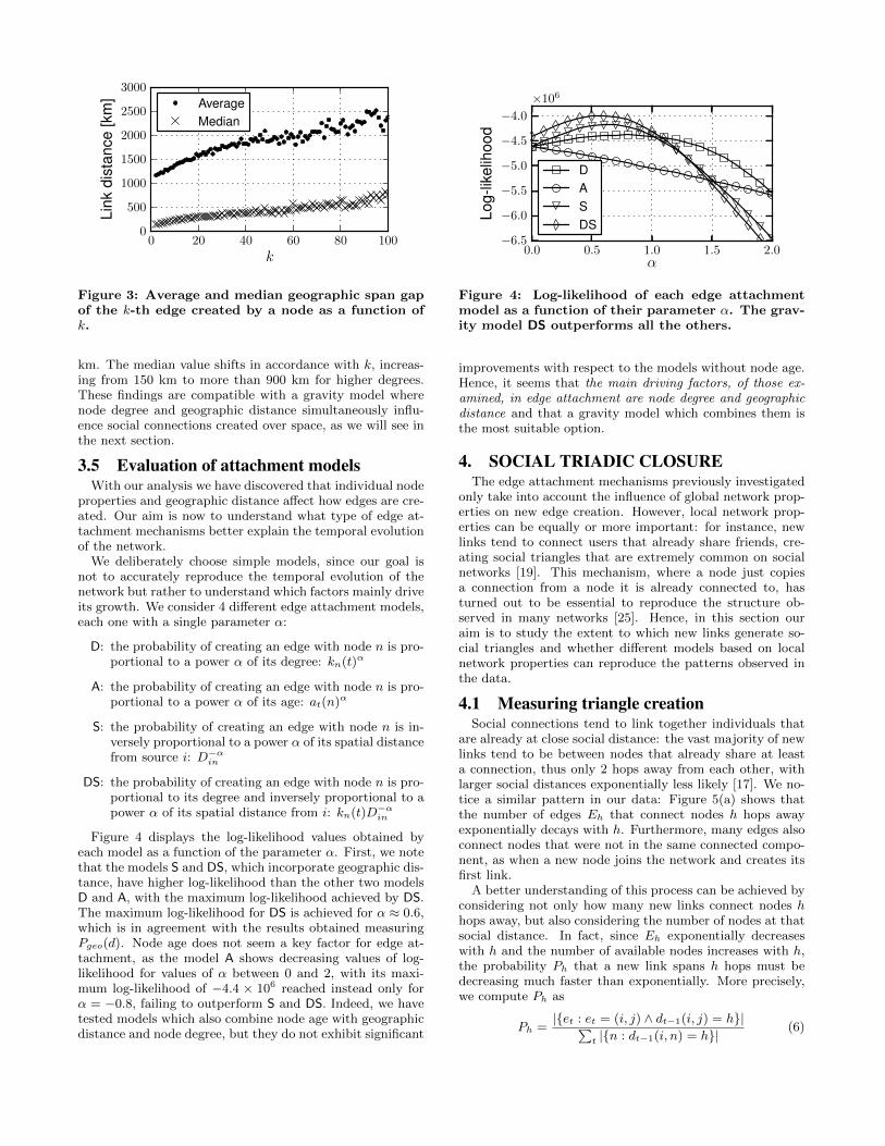
A consequence of the gravity model is that nodes withhigher degrees tend to attract longer links: thus, we defineλi(k) as the geographic length of the k-th edge created byuser i and we study λ(k) for different values of k. The influ-ence of degree k on the geographic properties of social linksappears strong: as described in Figure 3, both the averageand the median value of the geographic length 〈λ(k)〉 of thek-th edge increase with k: while the average length of thefirst edge is about 1,100 km, the 100th edge is about 2,400
0 20 40 60 80 100
k
0
500
1000
1500
2000
2500
3000
Link
dist
ance
[km
] AverageMedian
Figure 3: Average and median geographic span gapof the k-th edge created by a node as a function ofk.
km. The median value shifts in accordance with k, increas-ing from 150 km to more than 900 km for higher degrees.These findings are compatible with a gravity model wherenode degree and geographic distance simultaneously influ-ence social connections created over space, as we will see inthe next section.
3.5 Evaluation of attachment modelsWith our analysis we have discovered that individual node
properties and geographic distance affect how edges are cre-ated. Our aim is now to understand what type of edge at-tachment mechanisms better explain the temporal evolutionof the network.
We deliberately choose simple models, since our goal isnot to accurately reproduce the temporal evolution of thenetwork but rather to understand which factors mainly driveits growth. We consider 4 different edge attachment models,each one with a single parameter α:
D: the probability of creating an edge with node n is pro-portional to a power α of its degree: kn(t)α
A: the probability of creating an edge with node n is pro-portional to a power α of its age: at(n)α
S: the probability of creating an edge with node n is in-versely proportional to a power α of its spatial distancefrom source i: D−α
in
DS: the probability of creating an edge with node n is pro-portional to its degree and inversely proportional to apower α of its spatial distance from i: kn(t)D−α
in
Figure 4 displays the log-likelihood values obtained byeach model as a function of the parameter α. First, we notethat the models S and DS, which incorporate geographic dis-tance, have higher log-likelihood than the other two modelsD and A, with the maximum log-likelihood achieved by DS.The maximum log-likelihood for DS is achieved for α ≈ 0.6,which is in agreement with the results obtained measuringPgeo(d). Node age does not seem a key factor for edge at-tachment, as the model A shows decreasing values of log-likelihood for values of α between 0 and 2, with its maxi-mum log-likelihood of −4.4 × 10⁶ reached instead only forα = −0.8, failing to outperform S and DS. Indeed, we havetested models which also combine node age with geographicdistance and node degree, but they do not exhibit significant
0.0 0.5 1.0 1.5 2.0α
−6.5
−6.0
−5.5
−5.0
−4.5
−4.0
Log-
likel
ihoo
d
×106
DASDS
Figure 4: Log-likelihood of each edge attachmentmodel as a function of their parameter α. The grav-ity model DS outperforms all the others.
improvements with respect to the models without node age.Hence, it seems that the main driving factors, of those ex-amined, in edge attachment are node degree and geographicdistance and that a gravity model which combines them isthe most suitable option.
4. SOCIAL TRIADIC CLOSUREThe edge attachment mechanisms previously investigated
only take into account the influence of global network prop-erties on new edge creation. However, local network prop-erties can be equally or more important: for instance, newlinks tend to connect users that already share friends, cre-ating social triangles that are extremely common on socialnetworks [19]. This mechanism, where a node just copiesa connection from a node it is already connected to, hasturned out to be essential to reproduce the structure ob-served in many networks [25]. Hence, in this section ouraim is to study the extent to which new links generate so-cial triangles and whether different models based on localnetwork properties can reproduce the patterns observed inthe data.
4.1 Measuring triangle creationSocial connections tend to link together individuals that
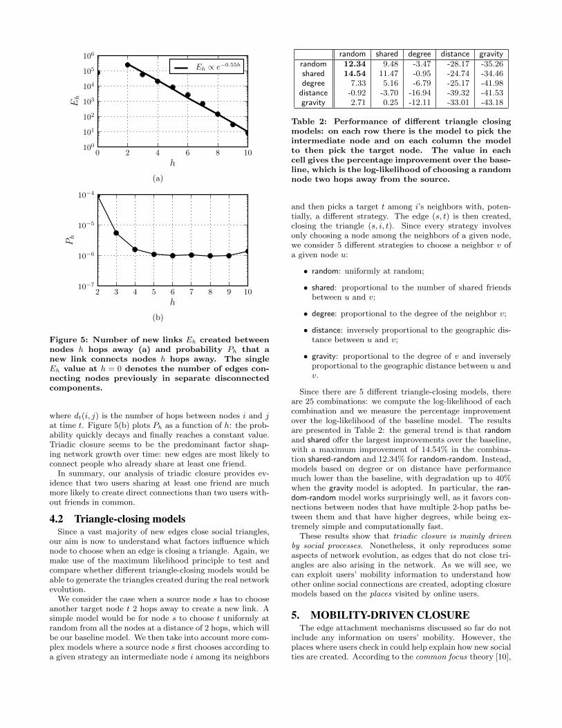
are already at close social distance: the vast majority of newlinks tend to be between nodes that already share at leasta connection, thus only 2 hops away from each other, withlarger social distances exponentially less likely [17]. We no-tice a similar pattern in our data: Figure 5(a) shows thatthe number of edges Eh that connect nodes h hops awayexponentially decays with h. Furthermore, many edges alsoconnect nodes that were not in the same connected compo-nent, as when a new node joins the network and creates itsfirst link.
A better understanding of this process can be achieved byconsidering not only how many new links connect nodes hhops away, but also considering the number of nodes at thatsocial distance. In fact, since Eh exponentially decreaseswith h and the number of available nodes increases with h,the probability Ph that a new link spans h hops must bedecreasing much faster than exponentially. More precisely,we compute Ph as
Ph =|{et : et = (i, j) ∧ dt−1(i, j) = h}|∑
t |{n : dt−1(i, n) = h}| (6)
0 2 4 6 8 10
h
100
101
102
103
104
105
106
Eh
Eh ∝ e−0.55h
(a)
2 3 4 5 6 7 8 9 10
h
10−7
10−6
10−5
10−4
Ph
(b)
Figure 5: Number of new links Eh created betweennodes h hops away (a) and probability Ph that anew link connects nodes h hops away. The singleEh value at h = 0 denotes the number of edges con-necting nodes previously in separate disconnectedcomponents.
where dt(i, j) is the number of hops between nodes i and jat time t. Figure 5(b) plots Ph as a function of h: the prob-ability quickly decays and finally reaches a constant value.Triadic closure seems to be the predominant factor shap-ing network growth over time: new edges are most likely toconnect people who already share at least one friend.
In summary, our analysis of triadic closure provides ev-idence that two users sharing at least one friend are muchmore likely to create direct connections than two users with-out friends in common.
4.2 Triangle-closing modelsSince a vast majority of new edges close social triangles,
our aim is now to understand what factors influence whichnode to choose when an edge is closing a triangle. Again, wemake use of the maximum likelihood principle to test andcompare whether different triangle-closing models would beable to generate the triangles created during the real networkevolution.
We consider the case when a source node s has to chooseanother target node t 2 hops away to create a new link. Asimple model would be for node s to choose t uniformly atrandom from all the nodes at a distance of 2 hops, which willbe our baseline model. We then take into account more com-plex models where a source node s first chooses according toa given strategy an intermediate node i among its neighbors
random shared degree distance gravityrandom 12.34 9.48 -3.47 -28.17 -35.26shared 14.54 11.47 -0.95 -24.74 -34.46degree 7.33 5.16 -6.79 -25.17 -41.98
distance -0.92 -3.70 -16.94 -39.32 -41.53gravity 2.71 0.25 -12.11 -33.01 -43.18
Table 2: Performance of different triangle closingmodels: on each row there is the model to pick theintermediate node and on each column the modelto then pick the target node. The value in eachcell gives the percentage improvement over the base-line, which is the log-likelihood of choosing a randomnode two hops away from the source.
and then picks a target t among i’s neighbors with, poten-tially, a different strategy. The edge (s, t) is then created,closing the triangle (s, i, t). Since every strategy involvesonly choosing a node among the neighbors of a given node,we consider 5 different strategies to choose a neighbor v ofa given node u:
• random: uniformly at random;
• shared: proportional to the number of shared friendsbetween u and v;
• degree: proportional to the degree of the neighbor v;
• distance: inversely proportional to the geographic dis-tance between u and v;
• gravity: proportional to the degree of v and inverselyproportional to the geographic distance between u andv.
Since there are 5 different triangle-closing models, thereare 25 combinations: we compute the log-likelihood of eachcombination and we measure the percentage improvementover the log-likelihood of the baseline model. The resultsare presented in Table 2: the general trend is that randomand shared offer the largest improvements over the baseline,with a maximum improvement of 14.54% in the combina-tion shared-random and 12.34% for random-random. Instead,models based on degree or on distance have performancemuch lower than the baseline, with degradation up to 40%when the gravity model is adopted. In particular, the ran-dom-random model works surprisingly well, as it favors con-nections between nodes that have multiple 2-hop paths be-tween them and that have higher degrees, while being ex-tremely simple and computationally fast.
These results show that triadic closure is mainly drivenby social processes. Nonetheless, it only reproduces someaspects of network evolution, as edges that do not close tri-angles are also arising in the network. As we will see, wecan exploit users’ mobility information to understand howother online social connections are created, adopting closuremodels based on the places visited by online users.
5. MOBILITY-DRIVEN CLOSUREThe edge attachment mechanisms discussed so far do not
include any information on users’ mobility. However, theplaces where users check in could help explain how new socialties are created. According to the common focus theory [10],

0 2 4 6 8 10
h
100
101
102
103
Dh
[km
]
Figure 6: Average geographic distance Dh of newlinks created between nodes h hops away. The sin-gle value at h = 0 denotes the average geographicdistance of links connecting nodes previously in sep-arate disconnected components.
individuals who visit the same places tend to establish newsocial connections. In this section we measure the impactthat users’ mobility has on network evolution. In agreementwith the common focus theory, we study edge attachmentmechanisms that connect users that visit the same places.
5.1 Measuring mobility-based attachmentIn our Gowalla traces, 32.28% of all new edges are estab-
lished between users that share at least one common place.In particular, about 10% of new links are created betweenusers that do share common places, but no common friends.This means that adopting only social triadic closure mech-anisms would fail to reproduce that users create new socialconnections beyond their 2-hop neighborhood.
The importance of social ties that connect users withoutfriends in common is confirmed when we examine the aver-age geographic distance Dh of all new edges that connectnodes previously h hops away, shown in Figure 6. There isan evident trend: social connections at shorter social dis-tance tend to have higher geographic distances, while linksspanning more hops have lower spatial distance. A potentialexplanation is that both social and spatial factors tend toaffect the edge creation process: a new link is created eitherbetween users sharing friends, even if they are far from eachother, or between spatially close users, even if they have nofriends in common. In particular, geographic proximity be-comes complementary to social closeness: both factors areshaping the network, but in different ways. The challenge isto go beyond geographic distance when modeling the evolu-tion of the network: mobility-based attachment provides theadditional source of information, based on the places visitedby users. Such information may be important to model net-work evolution, since it provides more accurate geographicinformation than users’ home locations.
5.2 Mobility-driven closure modelsWe consider mobility-driven closure models to be two-step
processes. A source node s first selects a place p ∈ Ps, wherePs is the set of all places where node s has checked in; then,given place p a target note t ∈ Qp is selected, where Qp isthe set of all nodes that have checked in at place p. Weconsider different strategies that a node u adopts to select aplace p from the set Pu:
• random: uniformly at random;
• friends: proportional to the number of user u’s friendsthat have visited p;
• user-checkins: proportional to the number of check-insmade by user u at p;
• tot-checkins: proportional to the total number of check-ins made at p by all users;
• tot-users: proportional to the total number of userswho have checked in at p;
• place-distance: inversely proportional to the distancebetween user u’s home location and p;
• place-gravity: proportional to the total number of check-ins made by all users at place p and inversely propor-tional to the distance between user u’s home locationand p.
Given a selected place p, we then consider another set ofstrategies to select a target user t from Qp:
• random: uniformly at random;
• degree: proportional to user t’s degree;
• deg-diffusion: proportional to user t’s degree and in-versely proportional the logarithm of user t’s total num-ber of visited places;
• user-checkins: proportional to user t’s number of check-ins at p;
• tot-checkins: proportional to user t’s total number ofcheck-ins;
• inv-tot-checkins: inversely proportional to user t’s totalnumber of check-ins;
• distance: inversely proportional to the distance be-tween user t’s home location and p;
• gravity: proportional to user t’s degree and inverselyproportional to the distance between user t’s home lo-cation and p.
To test and evaluate mobility-driven models we use againthe maximum likelihood principle; we only evaluate the like-lihood that a model has to reproduce real edge attachmentswhere the source and target nodes share at least one place.We adopt a baseline model that selects at random targetusers from the set of all users that share places with thesource. Table 3 presents the results for all the possible com-binations.
In general, in the first step the best improvement is givenby selecting a popular place that has already been visitedby many users, friends or not. For the second step, nodedegree plays an important role, akin to a local preferentialattachment. The greatest improvement over the baselineis provided by first selecting a place that has been visitedmany times (tot-checkins) and then choosing a node propor-tionally to its degree “diffused” over the number of visitedplaces (deg-diffusion). This mobility measure corrects for thefact that popular users that visit only a few places might bemore related to that place, thus enticing other visitors to

random degree deg-diffusion user-checkins tot-checkins inv-tot-checkins distance gravityrandom 0.28 6.88 9.24 0.16 -17.02 -4.51 -19.36 -7.04friends 4.70 11.60 13.63 4.74 -10.63 -1.56 -14.88 -1.71
user-checkins 0.05 6.59 8.94 -0.03 -17.27 -4.80 -19.69 -7.41tot-checkins 6.09 13.13 15.18 6.14 -9.29 0.04 -13.15 -0.02
tot-users 5.10 12.33 14.33 5.16 -9.96 -1.08 -14.19 -0.84place-distance -23.41 -15.57 -13.21 -23.56 -40.82 -28.27 -43.67 -30.17place-gravity 0.37 7.22 9.46 0.32 -16.26 -5.29 -19.60 -6.81
Table 3: Performance of mobility-driven closure models: on each row there is a model to pick the intermediateplace and on each column a model to then pick the target node. The value in each cell gives the percentageimprovement over the baseline, which is the log-likelihood of choosing a node at random among all the nodesthat share at least one place with the source.
0 100 200 300 400 500
Node lifespan (days)
10−4
10−3
10−2
10−1
100
CC
DF
Figure 7: Complementary Cumulative DistributionFunction (CCDF) of node lifespan and exponentialfit.
connect. The tot-checkins-degree model has a similar butslightly inferior performance, yet it is simpler and computa-tionally faster.
In addition to the models presented in Table 3, we exper-imented with variations of tot-users and tot-checkins wherewe use a probability of attachment inversely proportionalto the total number of users or check-ins. All these modelsprovided inferior performance compared to the baseline.
6. TEMPORAL EVOLUTIONIn this section we study how users create new connections
as they spend more time on the network. We study theamount of time users remain active for, their lifespan; then,we investigate the inter-edge temporal gap between the cre-ation of consecutive edges. In this section we consider onlyusers that joined the service after our measurement processstarted, in order to observe their behavior from the very firstmoment.
6.1 Node lifespanWe define the lifespan of a node as the difference between
the time the node created the last and the first edge. Fig-ure 7 plots the distribution of lifespan for all users: thedistribution shows an approximately exponential behavior,with a deviation only at longer lifespans for few users whowere early adopters and started using the service from thevery first days. The fit is reasonably accurate for a widerange of lifespan values.
100 101 102
δ(1) [days]
10−4
10−3
10−2
10−1
100
PD
F
Trunc. power-lawShifted exp.Power-law
Figure 8: Probability Distribution Function (PDF)of δ(1), the temporal gap elapsing between the timewhen the first and the second edge are created bya user. The fits show a power law, an exponentiallytruncated power law and a shifted exponential.
6.2 Inter-edge temporal gapDifferent users can show significant differences in the pace
they add new edges: users with higher degree create newties at a faster rate. Thus, we study δi(k), the temporal gapbetween the k-th and k + 1-th edges of user i, for differentvalues of k.
Figure 8 displays the probability distribution of δ(1), theamount of time between the first and the second edges cre-ated by a user. Even though many users add their secondedge after a few days, some wait for several weeks. The dis-tribution can be reproduced by different functional forms:an exponentially truncated power law δ(1)−α1exp(−δ(1)/β1)yields a slightly higher log-likelihood than a pure power-law,a shifted exponential and an exponential; the average log-likelihood improvement over the exponential fit is about 5%.This result also holds for different values of k.
Then, we study the effect of current degree k: in partic-ular, we are interested in how the probability distributionof δ(k) changes with k. A first indication is given in Fig-ure 9(a), which plots the average temporal gap 〈δ(k)〉 be-tween the k-th and k + 1-th edges for different values of k:users with higher degrees tend to wait, on average, for ashorter amount of time. In fact, users wait on average 20days before adding their second edge but only 7 days whenthey have about 100 friends. While αk tends to be unre-lated to k, the exponential cut-off βk becomes smaller ask grows larger, as seen in Figure 9(b). The final effect isthat nodes with higher degrees are more likely to wait for

0 20 40 60 80 100
k
6
8
10
12
14
16
18
20
22
〈δ(k
)〉
(a)
0 20 40 60 80 100
k
0
10
20
30
40
50
60
70
80
βk
(b)
Figure 9: Average temporal gap 〈δ(k)〉 between thek-th and k + 1-th edge (a) and exponential cut-off βk (b) in the truncated power law p(δ(k)) ∝δ(k)−αkexp(−δ(k)/βk), as a function of node degreek.
a shorter time span, as the truncated tail of the power lawP (δ(k)) increasingly constrains larger gap values.
It is not surprising that nodes with higher degree add linksat a higher pace: given a fixed temporal period, as in ourmeasurement, higher degree nodes add more links than lowerdegree ones, so their activity has to be faster in the sametemporal period. Nonetheless, this heterogeneous temporalbehavior is crucial to foster the heterogeneity observed inthe degree distribution of social systems [17].
7. PUTTING IT ALL TOGETHER:NEW MODELS
We have seen that a gravity-based attachment, combin-ing spatial distance and node degree, influences how newedges are created (in Section 3). At the same time, wehave discussed that triadic and mobility-based closure aremainly shaped by social factors rather than geographic ones(in Section 4 and 5). These two mechanisms seem to becomplementary: while the gravity attachment is responsiblefor edges connecting together different parts of the network,the closure mechanisms seem involved in the creation of lo-cal edges between nodes that already share either a friendor a place. Finally, we have analyzed how nodes tend tobecome faster and faster in creating new edges as they getmore connections (in Section 6). Building on all these re-
sults, our aim is now to define network growth models whichare able to reproduce the spatial and social properties ob-served in the real network. We stress that the goal of ourmodels is not to accurately reproduce the network or pre-dict edge creation events, but to describe the fundamentalmechanisms affecting user behavior.
7.1 Model definitionFollowing the methodology presented in [17], we describe
our model as a simple algorithm to grow a network one node,and one edge, at a time. Our model combines global attach-ment mechanisms and local closure mechanisms:
1. A new node u joins the network according to a certainarrival discipline and positions itself over the space;
2. A new node u samples its lifetime from an exponentialdistribution;
3. Node u adds its first edge to node v according to aglobal connection model (preferential or gravity-basedattachment);
4. A node with degree k samples a time gap δ from a dis-tribution p(δ(k)) ∝ δ(k)−αkexp(−δ(k)/βk) and thengoes to sleep for δ time steps;
5. When a node wakes up, if its lifetime has not expiredyet it creates a new edge: with probability p the nodeuses the random−random social triangle-closing model,otherwise it uses the tot-checkins − degree mobility-based closure.
6. The node repeats step 4.
The probability p allows us to assess the impact that thelocal closure models have on overall accuracy. In particular,we adopt two variations: we use p = 1 so that the modelonly includes social triadic closure, and we adopt p = 0.66to introduce also mobility-driven closure (this value is mo-tivated by the observed frequency of edge attachments inthe real data). This yields a total of 4 different combina-tions: gravity-based (G), gravity-based with mobility-drivenclosure (GM), preferential attachment (P) and preferentialattachment with mobility-driven closure (PM).
Finally, we note that local closure models only accountfor about two-thirds of all new social links. The remainingfraction includes ties between users that do not share com-mon friends and that do not visit the same places. Thus, weintroduce a variation into our models whose aim is to adoptglobal attachment models also during a node’s lifetime, andnot only in step 3. In more detail, when a node wakes up instep 5, with probability q = 0.33 it creates an edge accordingto the global attachment mechanisms; otherwise, the modelproceeds as defined. This yields 4 additional model combi-nations, for a total of 8 combinations. We will present ourresults separately for combinations that do and do not trig-ger global attachment mechanisms during a node’s lifetime.
7.2 EvaluationTo test our model we take the real network at the begin-
ning of our measurement, Gt, and simulate its growth byadding the missing nodes and check-ins, with their real geo-graphic locations, and the check-ins according to when andwhere they happen in the real network. However, once they

100 101 102 103 104
Node degree
10−5
10−4
10−3
10−2
10−1
100
PD
FDataGP
GMPM
(a) Without global attachment
100 101 102 103 104
Node degree
10−5
10−4
10−3
10−2
10−1
100
PD
F
DataGP
GMPM
(b) With global attachment
Figure 10: Probability distribution function (PDF) of node degree for real data and different models: gravity-based (G), gravity-based with mobility-driven closure (GM), preferential attachment (P), preferential attach-ment with mobility-driven closure (PM).
100 101 102 103 104
Link length [km]
0.0
0.2
0.4
0.6
0.8
1.0
CD
F
DataGP
GMPM
(a) Without global attachment
100 101 102 103 104
Link length [km]
0.0
0.2
0.4
0.6
0.8
1.0
CD
F
DataGP
GMPM
(b) With global attachment
Figure 11: Cumulative distribution function (CDF) of link geographic length for real data and differentmodels: gravity-based (G), gravity-based with mobility-driven closure (GM), preferential attachment (P),preferential attachment with mobility-driven closure (PM).
join the network they add new edges according to our algo-rithmic model. We stop the evolution when the simulatednetwork has the same number of nodes as the real one, GT .
All 8 model combinations are run 10 times with differ-ent random seeds and then their properties are averagedover all these realizations. When computing the propertiesshown in Figures 10, 11, 12 and 13 we only consider edgesadded after the start of our measurement period, both in thereal network and in the simulated models, to avoid that theproperties of the initial graph Gt dominate the final result.
The degree distribution observed in the real network andthe two models are depicted in Figure 10: all models are ableto reproduce the distribution, capturing the social proper-ties of the real network. There is no noticeable differencebetween models with and without global attachment. How-ever, as shown in Figure 11, the probability distribution oflink geographic length is closer to the real one for gravity-based model, while models P and PM have links with longergeographic length. We note that models with global attach-ment have more similar characteristics than those without:the effect is that models G and GM reproduce better the
real distribution, while social links created by models P andPM tend to span longer geographic distance. This suggestsa positive effect of a gravity-based global attachment mech-anism on the accuracy of the model.
Another important difference between the gravity-basedand the preferential attachment models is highlighted byconsidering the geometric average distance of the links of auser as a function of the node degree. As seen in Figure 12,models G and GM show an increasing trend as the originaldata, while, on the contrary, models P and PM have weakercorrelation between node degree and geographic length ofthe links. Again, global attachment emphasizes the dif-ference between gravity-based and preferential attachmentmodels, with the first ones reproducing more accurately thereal trend. A similar behavior is observed in Figure 13 thepreferential attachment models create triangles on a muchwider geographic scale than models G and GM, which arecloser to the real data.
We note that when mobility-based closure is used resultsalways marginally improve with respect to models with onlysocial triadic closure. This performance increase can be

100 101 102 103
Node degree
102
103
104
Frie
nddi
stan
ce[k
m]
DataGP
GMPM
(a) Without global attachment
100 101 102 103
Node degree
102
103
104
Frie
nddi
stan
ce[k
m]
DataGP
GMPM
(b) With global attachment
Figure 12: Average geographic friend distance as a function of node degree for real data and different models:gravity-based (G), gravity-based with mobility-driven closure (GM), preferential attachment (P), preferentialattachment with mobility-driven closure (PM).
100 101 102 103 104
Node degree
101
102
103
104
105
Tria
ngle
leng
th[k
m]
DataGP
GMPM
(a) Without global attachment
100 101 102 103 104
Node degree
101
102
103
104
105
Tria
ngle
leng
th[k
m]
DataGP
GMPM
(b) With global attachment
Figure 13: Average geographic triangle length as a function of node degree for real data and different models:gravity-based (G), gravity-based with mobility-driven closure (GM), preferential attachment (P), preferentialattachment with mobility-driven closure (PM).
attributed to the latent geographic information embeddedin user check-ins. The effect of global attachment is evenstronger, as it enhances the accuracy of gravity-based mod-els, while also reducing the validity of preferential attach-ment models. These results confirm that the effect of ge-ographic distance can not be neglected when social net-works are studied and modeled: preferential attachmentmechanisms need to be modified into gravity-based mecha-nisms, which are able to correctly balance the effects of nodeattractiveness and the connection costs imposed by spa-tial distance. Furthermore, mobility-based closure improvesmodel accuracy, offering additional information about thegeographic whereabouts of online users.
7.3 ImplicationsThe importance of our findings goes beyond the definition
of accurate models of network evolution. Our results showthat the effect of geographic distance cannot be neglectedwhen online social networks are studied and modeled. In
reality, preferential attachment and triadic closure togetherare already able to reproduce the global social propertiesobserved in real social networks, namely the degree distribu-tion and the level of clustering. However, neglecting spatialinformation about where users are located fails to accountfor the effect of distance. In real systems users preferentiallyconnect over short distances, resulting in a considerable frac-tion of short-range ties; instead, ignoring spatial constraintswould predict an unlikely majority of long-range connec-tions. This goes against empirical evidence, both in offlineand online social systems.
Our findings support the idea that distance has a simpleeffect on the creation of social ties: the probability of connec-tion between two individuals decreases as a negative power ofthe spatial distance between them. Yet, this effect must becombined with a process based on“popularity”or“visibility”that introduces heterogeneity across users, such as attach-ment to the best connected nodes, in order to fully recreatethe self-reinforcing mechanisms that lead to the scale-freedegree distributions observed in social graphs.
Gravity mechanisms provide an elegant and insightful way

of combining the effect of distance and the influence of socialfactors. Surprisingly, the influence of distance on the forma-tion of social triads appears negligible, as other factors be-come more important at this level. The main implication ofthe gravity mechanism is that one user may be interested inanother because the other user is hugely popular, regardlessof their spatial distance, or because the other user is spa-tially close, regardless of popularity and importance. Thesemechanisms can be adopted in scenarios where the futureevolution of an online social graph has to be estimated: someexamples include security mechanisms for online services [1],the design of distributed storage solutions for massive socialgraphs [24] and the delivery of user-generated content [29].
The overall picture is that proximity both over physicaland social dimensions fosters the creation of new social links;the result is that the likelihood of a new connection increaseswhen two individuals share many other connections or whentwo individuals are close to each other. We also point outthat no friend recommendation mechanism was in place onthe online service under analysis during the measurementperiod.
This dual role of proximity has promising applications in awide range of systems. In particular, despite the abundanceof friend recommendation services, only few of them haveincluded spatial closeness in their systems [8, 27]. Our workprovides new insights for further research in this direction.
8. RELATED WORKThe temporal patterns of network evolution have been the
focus of many studies and several models have been put for-ward to describe the basic mechanisms that drive networkgrowth. A set of works studied the evolution of online socialnetworks, discussing the densification and diameter reduc-tion observed during the growth of the graph [11, 15]. Eventhough online social graphs tend to be have an heteroge-neous degree distribution in agreement with the preferentialattachment principle, these findings highlighted that, in so-cial networks, different mechanisms seems to be in place.More in detail, Leskovec et al. [18] propose a “forest-fire”copying process: when a new node joins the network andconnects to a first neighbor, it starts recursively creatingnew links among the neighbors of the first neighbor, effec-tively copying the connection already in place. This processmixes preferential attachment, as more connected nodes aremore likely to be selected, and transitivity, which fostersnew connections between nodes in social proximity. Thisconfirms the importance that triadic closure holds for theevolution of social graphs, as we have seen in our results.
Other works have also been focusing on triadic closure:Simmel noted that people sharing many friends might bemore likely to become connected [28]. This effect was thenmeasured in online social networks [19, 14] and included ingrowth models. With respect to these results, our work ex-plores, for the first time, the effect of spatial distance onnetwork evolution: specifically, we study how distance influ-ences preferential attachment and triadic closure.
Other works have been focusing on general models for spa-tial networks. One of the earliest examples is the Waxmanmodel, where nodes are distributed at random over spaceand then connected with probability exponentially decreas-ing with distance [30]. The Waxman model has also beenmodified as a growth model, where new nodes join the net-
work and connect with a similar rule [12]. Barthelemy pro-posed to combine preferential attachment with spatial dis-tance, studying how the resulting graphs move away frombeing scale-free as the effect of spatial distance is increased [4],albeit this case only considered an exponential decay withdistance as in the original Waxman model. Barrat et al. [3]also considered a similar model for weighted networks wherepreferential attachment is driven by the weight of the exist-ing connections and hampered by spatial distance. Whilethese works contain the initial ideas about including spatialinfluence in models of network growth, they were based onsystems such as transportation networks that lacked socialproperties. Hence, they tend to focus on an exponentialdecay of the probability of connection as a function of dis-tance, differently to what observed in social graphs, and theyignore properties arising from triadic closure. Our contribu-tion builds on these findings and bridges together several dif-ferent insights in order to obtain a suitable model for spatialsocial graphs.
Another set of works have investigated the spatial proper-ties of social networks: the influence of geographic distanceon social connections was firstly discussed in the LiveJournalcommunity [20]. This influence appears so important thatit can be exploited to predict where people live given theirfriends’ locations [1]. Other studies on mobile phone com-munication networks have found that social triangles tend toextend over large geographic distances [16] and that commu-nity detection approaches should take spatial distance intoaccount to achieve better results [9]. The fostering effect ofgeographic proximity on social ties has been demonstratedconsidering both purely spatial coincidences [7] and repeatedvisits to venues [27]. Our work extends these results by an-alyzing the effect of spatial distance not on the static struc-ture of social networks but on their temporal evolution.
Finally, we adopt the maximum likelihood methodologyfrom and we base our growth model on results presentedin [17], where the evolution of four different online social net-works was discussed. Again, our work differs as it addressesthe effect of geographic distance on the temporal mecha-nisms that govern network evolution, providing a more com-plete understanding of the factors driving social behavior.Furthermore, we describe a model of network growth whichsuccessfully reproduces both social and spatial propertiesobserved in online social graphs.
9. CONCLUSIONSIn this work we studied the evolution of the social graph
of a location-based service. We collected data about sociallinks created and places visited by users over a period of 4months and we studied the effect of spatial factors on thegrowth of the network.
We tested different models of edge attachment and wefound that on a global scale node degree and spatial distancesimultaneously affect how individuals create social connec-tions. On the other hand, on a local scale we studied triadicclosure models based on shared friends and on shared places:in these cases social factors are more important than spa-tial ones. Finally, we explored the temporal properties ofnetwork evolution, studying how much time users remainactive on the service and how the time elapsed between thecreation of consecutive social connections becomes shorteras users have more friends.

Based on our findings, we defined and tested networkgrowth models combining a global gravity-based attachmentwith local closure models based on shared friends and places.Our models are able to reproduce the structural and spatialproperties observed in the traces. Our results highlight ba-sic factors driving social network growth that could impact arange of research efforts and practical applications. Overall,this work builds up on previous results and provides furtherevidence that spatial factors should not be neglected whenstudying and modeling online social services.
AcknowledgmentsThis research was partly funded by a Google Research Award.
10. REFERENCES[1] L. Backstrom, E. Sun, and C. Marlow. Find me if you
can: improving geographical prediction with social andspatial proximity. In Proceedings of WWW’10, 2010.
[2] A.-L. Barabasi and R. Albert. Emergence of Scaling inRandom Networks. Science, 286(5439), 1999.
[3] A. Barrat, M. Barthelemy, and A. Vespignani. Theeffects of spatial constraints on the evolution ofweighted complex networks. Journal of StatisticalMechanics, (05), 2005.
[4] M. Barthelemy. Crossover from scale-free to spatialnetworks. Europhysics Letters, 63, 2003.
[5] M. Barthelemy. Spatial Networks. Physics Reports,499, 2011.
[6] V. Carrothers. A Historical Review of the Gravity andPotential Concepts of Human Interaction. Journal ofthe American Institute of Planners, 22, 1956.
[7] D. J. Crandall, L. Backstrom, D. Cosley, S. Suri,D. Huttenlocher, and J. M. Kleinberg. Inferring socialties from geographic coincidences. PNAS,107(52):22436–22441, 2010.
[8] J. Cranshaw, E. Toch, J. Hong, A. Kittur, andN. Sadeh. Bridging the gap between physical locationand online social networks. In Proceedings ofUbiComp’10, Copenhagen, Denmark, 2010.
[9] P. Expert, T. S. Evans, V. D. Blondel, andR. Lambiotte. Uncovering space-independentcommunities in spatial networks. PNAS,108(19):7663–7668, May 2011.
[10] S. L. Feld. The Focused Organization of Social Ties.American Journal of Sociology, 86(5):1015–1035, 1981.
[11] D. Fetterly, M. Manasse, M. Najork, and J. Wiener. Alarge-scale study of the evolution of web pages. InProceedings of WWW’03, 2003.
[12] M. Kaiser and C. C. Hilgetag. Spatial growth ofreal-world networks. PRE, 69:036103, Mar 2004.
[13] T. Karagiannis, C. Gkantsidis, D. Narayanan, andA. Rowstron. Hermes: clustering users in large-scalee-mail services. In Proceedings of SoCC’10, 2010.
[14] D. Krackhardt and M. S. Handcock. Heider vsSimmel: emergent features in dynamic structures. InProceedings of ICML’06, 2006.
[15] R. Kumar, J. Novak, and A. Tomkins. Structure andEvolution of Online Social Networks. In Proceedings ofKDD’06, 2006.
[16] R. Lambiotte, V. Blondel, C. Dekerchove, E. Huens,C. Prieur, Z. Smoreda, and P. Vandooren.Geographical dispersal of mobile communicationnetworks. Physica A, 387(21), 2008.
[17] J. Leskovec, L. Backstrom, R. Kumar, andA. Tomkins. Microscopic evolution of social networks.In Proceedings of KDD’08, 2008.
[18] J. Leskovec, J. Kleinberg, and C. Faloutsos. Graphsover time: densification laws, shrinking diameters andpossible explanations. In Proceedings of KDD’05, 2005.
[19] D. Liben-Nowell and J. Kleinberg. The link predictionproblem for social networks. In Proceedings ofCIKM’03, 2003.
[20] D. Liben-Nowell, J. Novak, R. Kumar, P. Raghavan,and A. Tomkins. Geographic routing in socialnetworks. PNAS, 102(33):11623–11628, 2005.
[21] R. N. Lichtenwalter, J. T. Lussier, and N. V. Chawla.New perspectives and methods in link prediction. InProceedings of KDD’10, 2010.
[22] A. Mislove, M. Marcon, K. P. Gummadi, P. Druschel,and B. Bhattacharjee. Measurement and Analysis ofOnline Social Networks. In Proceedings of IMC ’07,2007.
[23] J.-P. Onnela, S. Arbesman, M. C. Gonzalez, A.-L.Barabasi, and N. A. Christakis. Geographicconstraints on social network groups. PLoS ONE,6(4):e16939, 2011.
[24] J. M. Pujol, V. Erramilli, G. Siganos, X. Yang,N. Laoutaris, P. Chhabra, and P. Rodriguez. The littleengine(s) that could: scaling online social networks. InProceedings of SIGCOMM’10, 2010.
[25] D. M. Romero and J. Kleinberg. The Directed ClosureProcess in Hybrid Social-Information Networks, withan Analysis of Link Formation on Twitter. InProceedings of ICWSM’11, 2011.
[26] S. Scellato, A. Noulas, R. Lambiotte, and C. Mascolo.Socio-spatial Properties of Online Location-basedSocial Networks. In Proceedings of ICWSM’11, 2011.
[27] S. Scellato, A. Noulas, and C. Mascolo. Exploitingplace features in link prediction on location-basedsocial networks. In Proceedings of KDD’11, 2011.
[28] G. Simmel. The Sociology of Georg Simmel. The FreePress, 1908.
[29] S. Traverso, K. Huguenin, V. Trestian, I. Erramilli,N. Laoutaris, and K. Papagiannaki. TailGate:Handling Long-Tail Content with a Little Help fromFriends. In Proceedings of WWW’12, 2012.
[30] B. M. Waxman. Routing of multipoint connections.Selected Areas in Communications, 6(9):1617–1622,1988.
[31] M. P. Wittie, V. Pejovic, L. Deek, K. C. Almeroth,and B. Y. Zhao. Exploiting locality of interest inonline social networks. In Proceedings of CONEXT’10,2010.
[32] C. Wiuf, M. Brameier, O. Hagberg, and M. P. H.Stumpf. A likelihood approach to analysis of networkdata. PNAS, 103(20):7566–7570, 2006.