1

Evolution II.2. After The Origin.

”Some of the great scientists, carefully ciphering the evi-dences furnished by geology, have arrived at the convic-tion that our world is prodigiously old, and they may be right but Lord Kelvin is not of their opinion. He takes the cautious, conservative view, in order to be on the safe side, and feels sure it is not so old as they think. As Lord Kelvin is the highest authority in science now living, I think we must yield to him and accept his views.” [Mark Twain quoted by Burchfield (1990)]

2

Part I: The Eclipse of Darwinism. Between Scylla and Charybdis.

a. 1st edition of The Origin published 1859; 6th, 1872.

b. By 1867, Darwin’s argument had been shredded:

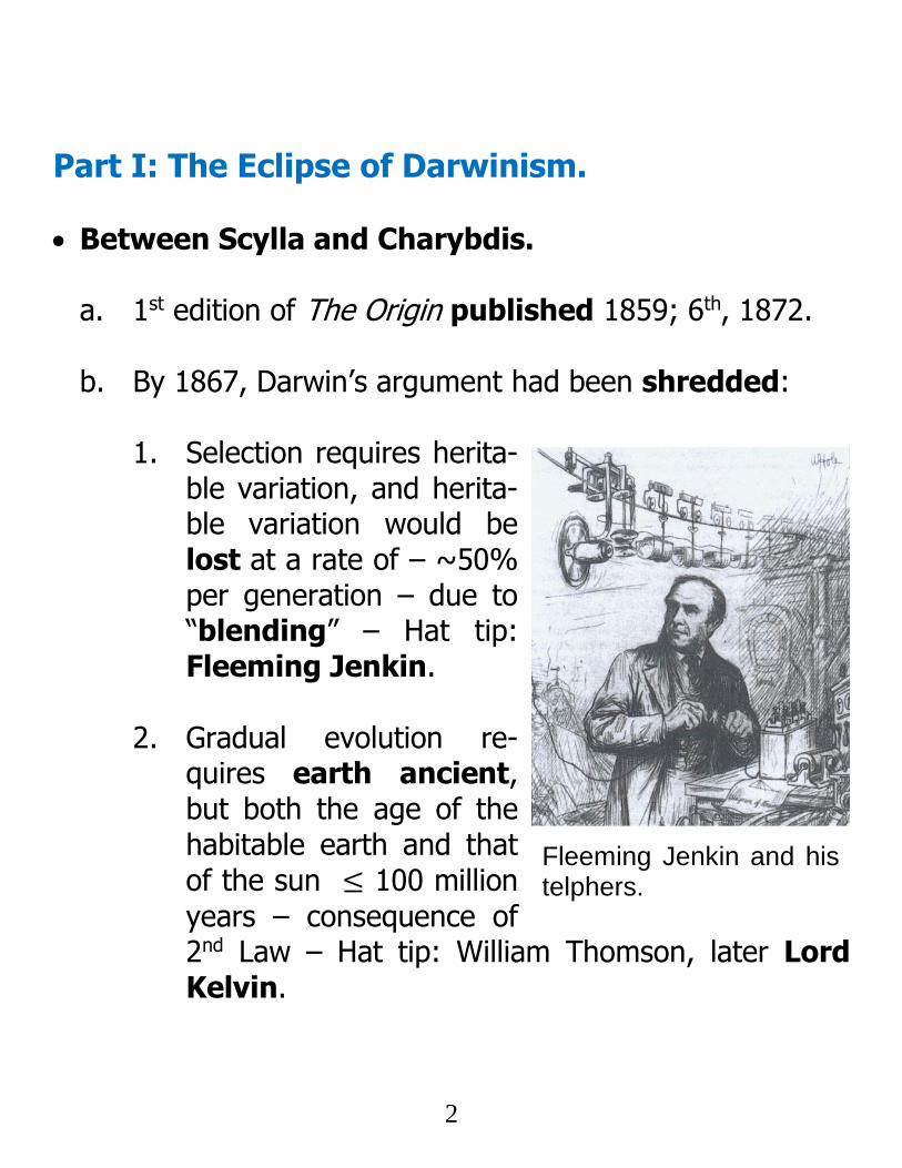
1. Selection requires herita-

ble variation, and herita-ble variation would be lost at a rate of – ~50% per generation – due to “blending” – Hat tip: Fleeming Jenkin.

2. Gradual evolution re-

quires earth ancient, but both the age of the habitable earth and that of the sun ≤ 100 million

years – consequence of 2nd Law – Hat tip: William Thomson, later Lord Kelvin.

Fleeming Jenkin and his telphers.

3

By the end of the 19th century: a. Many biologists confidently predicted the imminent

demise, if it was not already dead, of what by this time was called “Darwinism”.

b. There was renewed interest in both an inherent ten-dency to progress and IAC – so-called “Neo-Lamarckism”.

c. What kept the idea of evolution alive was increasing

evidence – anatomical, developmental and especially paleontological – for descent with modification.

d. But come the new century, Jenkin’s and Kelvin’s objec-

tions would be answered.

1. Particulate inheritance (the rediscovered lega-cy of Mendel) preserved heritable variation.

2. Earth’s true age, as ascertained by radiometric

dating, restored time in greater abundance than even Darwin and his acolytes had imagined.

4

Part II. Particulate Inheritance.

Mendelism.

a. “Experiments in Plant Hybridization” publ. in 1866.1

b. No one connected his work to the evolution debate.2

c. Mendelian inheritance rediscovered around 1900.

1. Initially believed to contradict gradual change.

2. Discrete characters seen as evidence for “salta-tion”, i.e., all at once origin of new species.

3. Wallace imagined Mendelian traits rare in nature

– variations of small effect the “stuff of evolution”.

d. In 1918, R. A. Fisher paved the way for the “Modern Synthesis” by showing that variability effectively continuous when many genes involved.

1 Available in translation at http://www.mendelweb.org/Mendel.html 2 Mendel’s opinion about evolution remains a subject of dispute. Some sug-gest that he viewed his results as supporting limits to variability, an opinion that would have placed him in the anti-evolution camp. Certainly, he disa-greed with Darwin’s claim that domestication promotes variability.

5

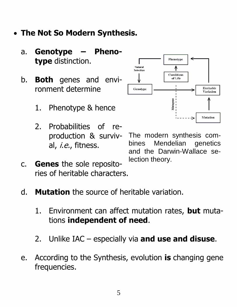
The Not So Modern Synthesis. a. Genotype – Pheno-

type distinction.

b. Both genes and envi-ronment determine

1. Phenotype & hence 2. Probabilities of re-

production & surviv-al, i.e., fitness.

c. Genes the sole reposito-

ries of heritable characters.

d. Mutation the source of heritable variation.

1. Environment can affect mutation rates, but muta-tions independent of need.

2. Unlike IAC – especially via and use and disuse.

e. According to the Synthesis, evolution is changing gene

frequencies.

The modern synthesis com-bines Mendelian genetics and the Darwin-Wallace se-lection theory.

6

Review of Diploid Genetics.

a. Most eukaryotes have a diploid stage – 2n chromo-somes and 2 copies of each autosomal gene.

b. Sex cells are haploid.

1. ⇒ an “alternation of

generations”.

2. Both haploid and diploid phases and can be uni- or multi-cellular.

c. Benefits of diploidy : 1. DNA repair (sister chromatids used as tem-

plates); 2. Production of new genotypes (recombination);

3. Dominance: Masks deleterious mutations; pre-

serves genetic variability.

4. Heterozygote advantage.

Alternation of generations in life cycle of a fern.

7

Review of Mendelian Inheritance.

a. Inheritance particulate – genes (Mendel’s “elemen-ten”) pass unchanged from generation to generation.

b. In diploid species, two

copies of each gene.

c. Genes segregate: each parent passes one copy to each offspring.

d. In accompanying exam-

ple, T (tall) is dominant. All F1 individuals tall. In F2 generation, short in-dividuals reappear. Tall: short ratio is 3:1.

e. If heterozygote pheno-

type intermediate, all F1 individuals intermediate; F2 ratios, 1:2:1.

f. Multiple characters assort independently – now

known to be the result of genes being on different chromosomes or of crossing over during meiosis.

Mendel demonstrated that inheritance is particulate. Genes can be masked, but not destroyed, by crossing.

8

Mitosis vs. meiosis. Products of mitosis (left) are diploid and ge-netically identical to parental cells. Products of meiosis (right) are haploid and not genetically identical to parental cells. Lack of iden-tity is due to crossing over.

9

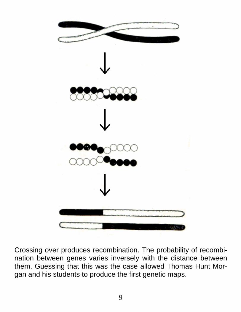
Crossing over produces recombination. The probability of recombi-nation between genes varies inversely with the distance between them. Guessing that this was the case allowed Thomas Hunt Mor-gan and his students to produce the first genetic maps.

10

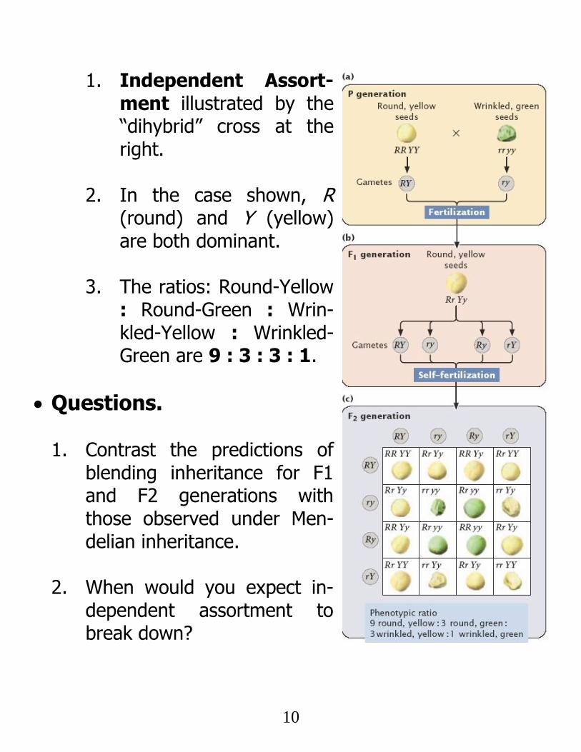
1. Independent Assort-ment illustrated by the “dihybrid” cross at the right.

2. In the case shown, R (round) and Y (yellow) are both dominant.

3. The ratios: Round-Yellow

: Round-Green : Wrin-kled-Yellow : Wrinkled-Green are 9 : 3 : 3 : 1.

Questions. 1. Contrast the predictions of

blending inheritance for F1 and F2 generations with those observed under Men-delian inheritance.

2. When would you expect in-

dependent assortment to break down?

11

g. Preceding can be summarized as Mendel’s Laws:3

1. Law of Segregation: Each hereditary char-acteristic is controlled by two ‘factors’ (Men-del’s Elementen), which pass into separate germ cells.

2. Law of Independent Assortment: Pairs of ‘factors’ segregate independently of each oth-er when germ cells are formed.

3 Adapted from Oxford Reference: http://www.oxfordreference.com/ . Search on Mendel’s Laws.

12

Mendel’s Motivation.

a. Hybridization had long been suggested as a

way of producing new species. b. Mendel interested in the stability of hybrids.

c. Calculated that continued selfing leads to elimi-

nation of heterozygotes, i.e., hybrids unstable – see Table next page.

1. Elimination of hybrids by selfing an extreme

example of finite population effects – see below.

2. Contrary to the idea that new species can be produced by hybridization as had been advo-cated by Lamarck.

3. Historical note: Mendel’s experiments were massive – the entire monastery recruited to help. Not the work of an amateur frolicking in the pea patch one summer.

13

Question.

3. Continue preceding table into the 5th generation.

Selfing Leads to Heterozygote Elimination. (Assume Four (4) Seeds per Cross)

Cross / Genotype AA Aa aa

1st Generation

Aa x Aa 1 2 1

1st Generation Total 1

(.25) 2

(.50) 1

(.25) 2nd Generation

AA x AA 4 0 0 2 (Aa x Aa) 2 4 2

aa x aa 0 0 4

2nd Generation Total 6

(.375) 4

(.25) 6

(.375) 3rd Generation

6 (AA x AA) 24 0 0 4 (Aa x Aa) 4 8 4 6 (aa x aa) 0 0 24

3rd Generation Total 28

(.4375) 8

(.125) 28

(.4375) 4th Generation

28 (AA x AA) 112 0 0 8 (Aa x Aa) 8 16 8 28 (aa x aa) 0 0 112

4th Generation Total 120

(.46875) 16

(.0625) 120

(.46875)

14

Population Genetics.

Hardy-Weinberg Law.

a. If mating random, gen-

otype frequencies de-termined by gene fre-quencies.

b. 1 locus; 2 alleles: A, a.

1. Three genotypes: AA, Aa, aa.

2. If gene frequencies p and q. H-W genotype frequencies are:

𝑝𝐴𝐴: 𝑝𝐴𝑎: 𝑝𝑎𝑎 = 𝑝2: 2𝑝𝑞: 𝑞2 (1)

3. Follows from the fact that the joint probability of two independent events is given by the prod-uct of the individual probabilities.

4. Since 𝒑 + 𝒒 = 𝟏, Eq(1) can also be written as

𝑝𝐴𝐴: 𝑝𝐴𝑎: 𝑝𝑎𝑎 = 𝑝2: 2𝑝(1 − 𝑝): (1 − 𝑝)2 (2)

H-W frequencies result from random mating between male and female parents.

15

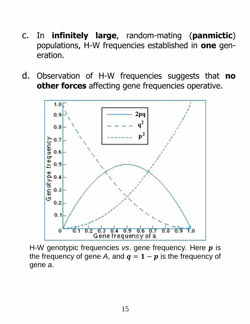
c. In infinitely large, random-mating (panmictic) populations, H-W frequencies established in one gen-eration.

d. Observation of H-W frequencies suggests that no other forces affecting gene frequencies operative.

H-W genotypic frequencies vs. gene frequency. Here 𝒑 is

the frequency of gene A, and 𝒒 = 𝟏 − 𝒑 is the frequency of gene a.

16

Questions.

4. Suppose there are three alleles, A1, A2, A3, with gene frequencies p, q, r. How many genotypes are there? What are their H-W frequencies?

5. Suppose the genotypic frequencies, 𝑝𝐴𝐴, etc., are 0.10, 0.50 and 0.40. a. What are the gene frequen-cies? b. Is the population in Hardy-Weinberg equilibri-um?

6. What might one conclude if a population is not in H-W

equilibrium?

Godfrey Hardy (left) and Wilhelm Weinberg (right) independently discovered the H-W equilibrium.

17

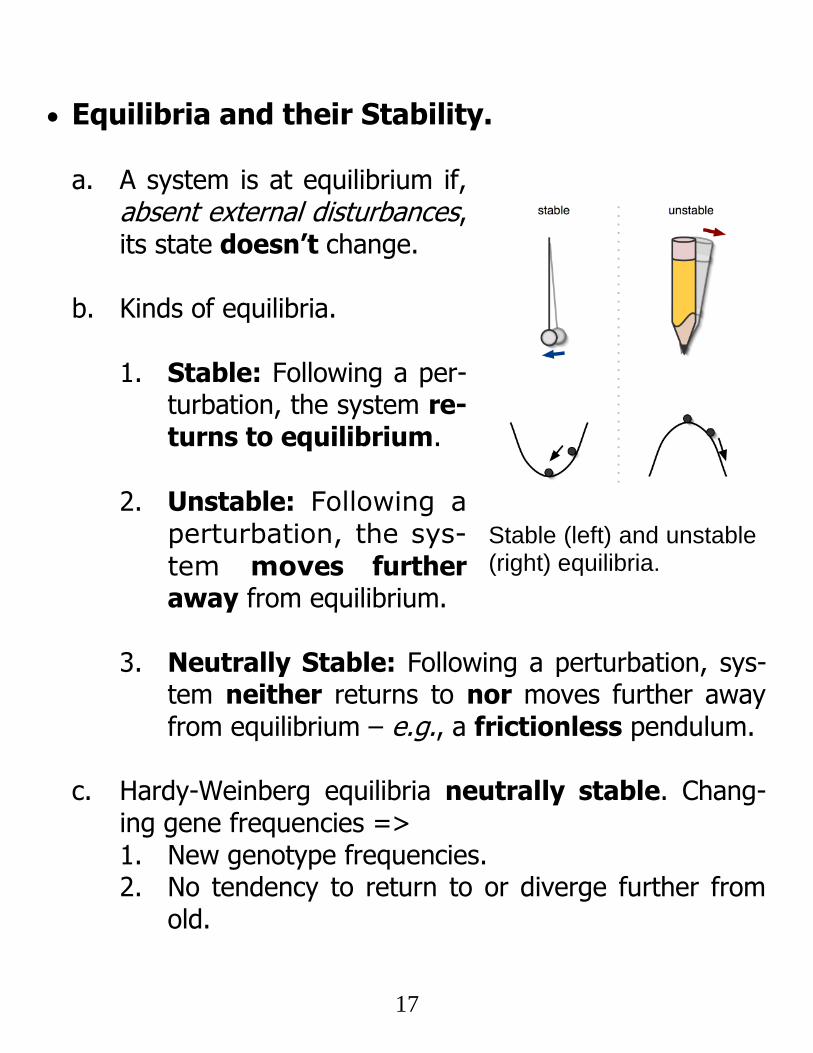
Equilibria and their Stability.

a. A system is at equilibrium if, absent external disturbances, its state doesn’t change.

b. Kinds of equilibria.

1. Stable: Following a per-

turbation, the system re-turns to equilibrium.

2. Unstable: Following a perturbation, the sys-

tem moves further away from equilibrium.

3. Neutrally Stable: Following a perturbation, sys-

tem neither returns to nor moves further away from equilibrium – e.g., a frictionless pendulum.

c. Hardy-Weinberg equilibria neutrally stable. Chang-

ing gene frequencies => 1. New genotype frequencies. 2. No tendency to return to or diverge further from

old.

Stable (left) and unstable (right) equilibria.

18

Forces that Affect Gene Frequencies. a. Selection. Different genotypes differentially repre-

sented in the next generation due to different proba-bilities of reproduction / survival.

b. Mutation. Changes in DNA base pair sequence – sometimes reversible (A ⇌ a); sometimes not.

c. Migration. Gene fre-

quency among immi-grants can differ from those among residents.

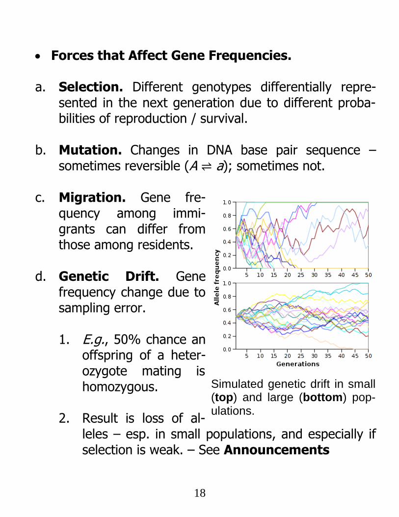
d. Genetic Drift. Gene

frequency change due to sampling error.

1. E.g., 50% chance an

offspring of a heter-ozygote mating is homozygous.

2. Result is loss of al-leles – esp. in small populations, and especially if selection is weak. – See Announcements

Simulated genetic drift in small (top) and large (bottom) pop-ulations.

19

e. Temporary small population size effects: 1. Founder effect.

2. Periodic bottlenecks of small population size.

Low genetic diversity in cheetahs is conjectured to have resulted from population size bottlenecks From O’Brian et al. 1987. PNAS. 84:508-511.

20

Finite Population Size, i.e., 𝑵 < ∞, Reduces Heterozygosity by Promoting Inbreeding.

a. Even if gene frequencies don’t change.

b. Recall Mendel’s selfing calculations. c. More generally, random mating implies crossings be-

tween individuals of differing degrees of related-ness – brother-sister, cousin-cousin, etc.

1. More closely related individuals, more likely to

share genes that are same by descent.

2. In infinite populations, everyone unrelated ⇒ H-

W genotypic frequencies.

3. In finite populations, all individuals related and therefore more likely to have same genes. Frequency of heterozygotes, 𝑝ℎ𝑒𝑡 → 0 as 𝑡 → ∞.

4. => more frequent expression of recessive, of-

ten deleterious, alleles – think hemophilia.

d. In real world, loss of alleles and heterozygosity coun-tered by mutation and migration.

21

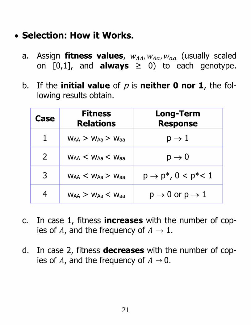
Selection: How it Works.

a. Assign fitness values, 𝑤𝐴𝐴, 𝑤𝐴𝑎, 𝑤𝑎𝑎 (usually scaled on [0,1], and always ≥ 0) to each genotype.

b. If the initial value of p is neither 0 nor 1, the fol-lowing results obtain.

c. In case 1, fitness increases with the number of cop-

ies of 𝐴, and the frequency of 𝐴 → 1.

d. In case 2, fitness decreases with the number of cop-

ies of 𝐴, and the frequency of 𝐴 → 0.

Case Fitness

Relations Long-Term Response

1 wAA > wAa > waa p 1

2 wAA < wAa < waa p 0

3 wAA < wAa > waa p p*, 0 < p*< 1

4 wAA > wAa < waa p 0 or p 1

22

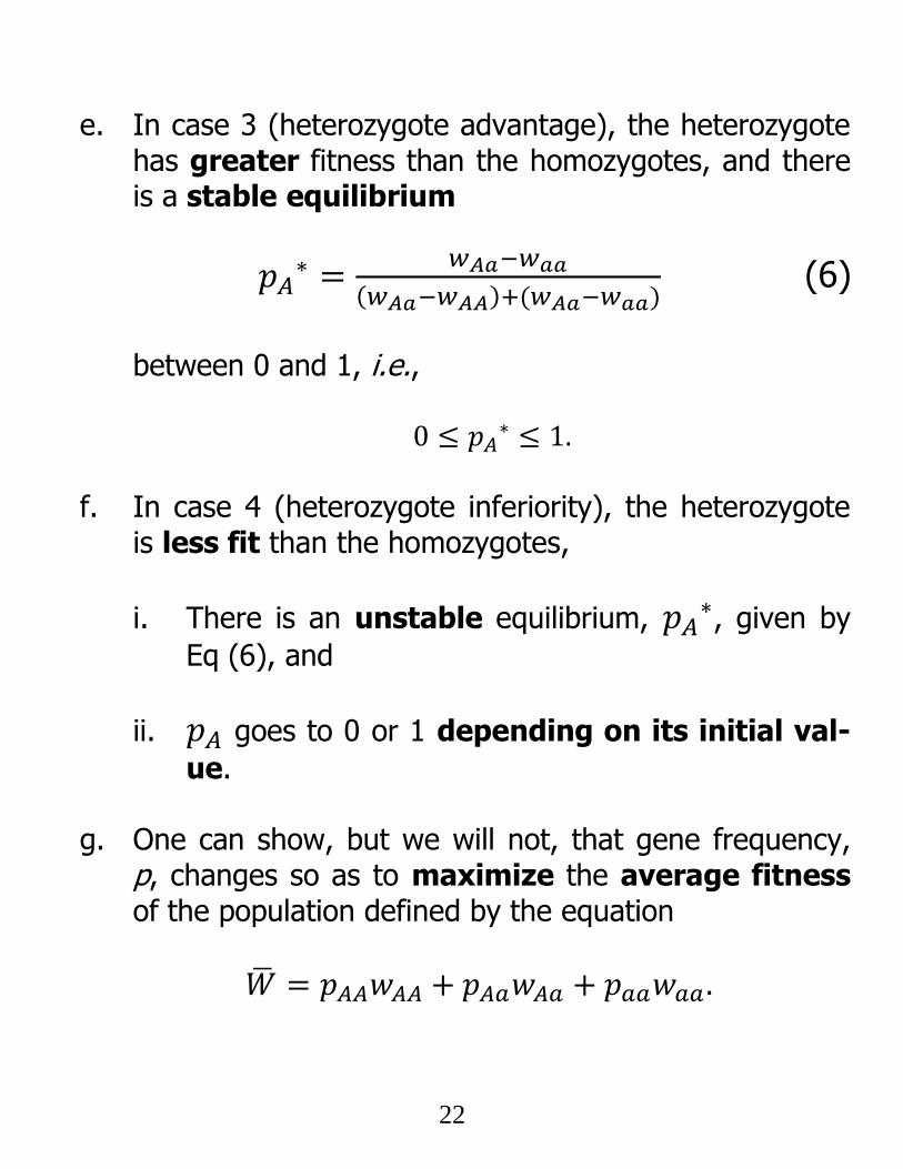
e. In case 3 (heterozygote advantage), the heterozygote has greater fitness than the homozygotes, and there is a stable equilibrium

𝑝𝐴∗ =

𝑤𝐴𝑎−𝑤𝑎𝑎

(𝑤𝐴𝑎−𝑤𝐴𝐴)+(𝑤𝐴𝑎−𝑤𝑎𝑎) (6)

between 0 and 1, i.e.,

0 ≤ 𝑝𝐴∗ ≤ 1.

f. In case 4 (heterozygote inferiority), the heterozygote

is less fit than the homozygotes,

i. There is an unstable equilibrium, 𝑝𝐴∗, given by

Eq (6), and

ii. 𝑝𝐴 goes to 0 or 1 depending on its initial val-

ue.

g. One can show, but we will not, that gene frequency, p, changes so as to maximize the average fitness of the population defined by the equation

�̅� = 𝑝𝐴𝐴𝑤𝐴𝐴 + 𝑝𝐴𝑎𝑤𝐴𝑎 + 𝑝𝑎𝑎𝑤𝑎𝑎 .

23

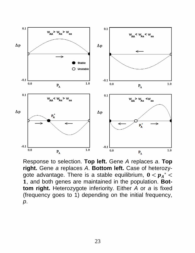
Response to selection. Top left. Gene A replaces a. Top right. Gene a replaces A. Bottom left. Case of heterozy-gote advantage. There is a stable equilibrium, 𝟎 < 𝒑𝑨

∗ <𝟏, and both genes are maintained in the population. Bot-tom right. Heterozygote inferiority. Either A or a is fixed (frequency goes to 1) depending on the initial frequency, p.

24

Questions.

7. In the case of heterozygote superiority, is p* stable or unstable?

8. In the case of heterozygote inferiority, is p* stable or unstable?

25

Malaria and Sickle Cell Anemia.

a. Hemoglobin (Hb) transports oxy-gen in red blood cells (RBCs).

b. Hb composed of four polypeptide

chains: two α- and two β-chains.

c. Substitution of one amino acid

in HbS/HbS individuals causes the β-chains of deoxygenated

HbS to polymerize, forming rigid fibers that collapse RBCs.

d. Cycling between polymerized

and de-polymerized states caus-es the cells to aggregate into fi-brous threads.

e. Threads obstruct small blood

vessels; causes hypoxia (lack of oxygen), tissue / organ dam-age.

f. E.g. , “cerebral malaria”, which is

often fatal.

Structure of Hb showing the four chains, each orga-nized about a heme group.

"Sickling" of an RBC drawn from an indi-vidual suffering from sickle cell anemia.

26

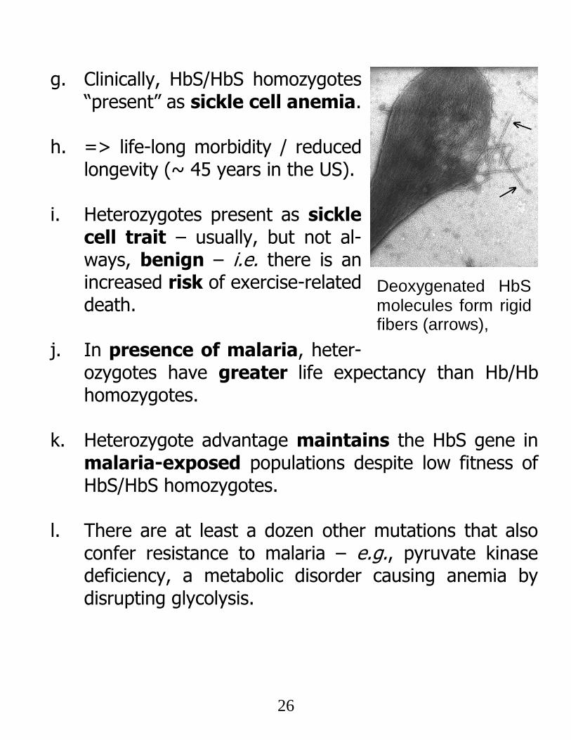
g. Clinically, HbS/HbS homozygotes “present” as sickle cell anemia.

h. => life-long morbidity / reduced longevity (~ 45 years in the US).

i. Heterozygotes present as sickle

cell trait – usually, but not al-ways, benign – i.e. there is an increased risk of exercise-related death.

j. In presence of malaria, heter-

ozygotes have greater life expectancy than Hb/Hb homozygotes.

k. Heterozygote advantage maintains the HbS gene in

malaria-exposed populations despite low fitness of HbS/HbS homozygotes.

l. There are at least a dozen other mutations that also

confer resistance to malaria – e.g., pyruvate kinase deficiency, a metabolic disorder causing anemia by disrupting glycolysis.

Deoxygenated HbS molecules form rigid fibers (arrows),

27

Questions.

9. Although estimated fitness values for the three geno-types, Hb/Hb, Hb/HbS and HbS/HbS, in the presence of malaria vary, the following numbers are probably reasonable:

wHb/Hb = 0.88; wHb/HbS = 1.0; wHbS/HbS = 0.14.

10. Using Eq (6), compute the equilibrium frequency of HbS.

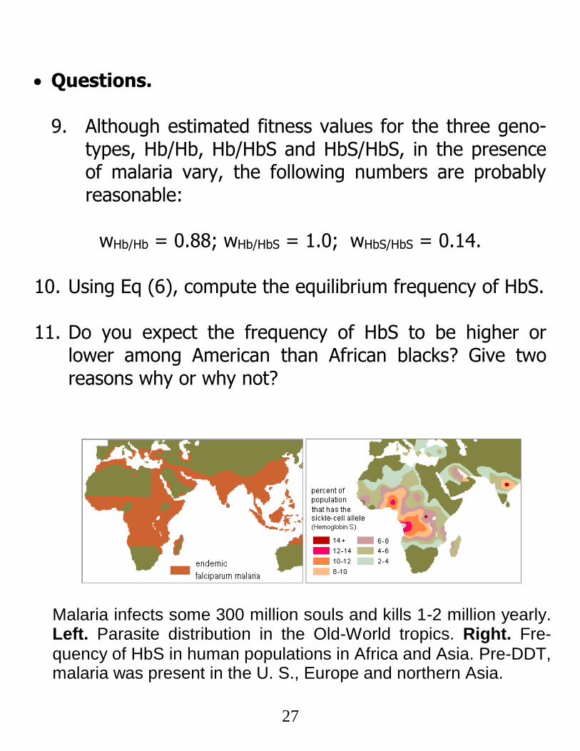
11. Do you expect the frequency of HbS to be higher or

lower among American than African blacks? Give two reasons why or why not?

Malaria infects some 300 million souls and kills 1-2 million yearly. Left. Parasite distribution in the Old-World tropics. Right. Fre-quency of HbS in human populations in Africa and Asia. Pre-DDT, malaria was present in the U. S., Europe and northern Asia.

28

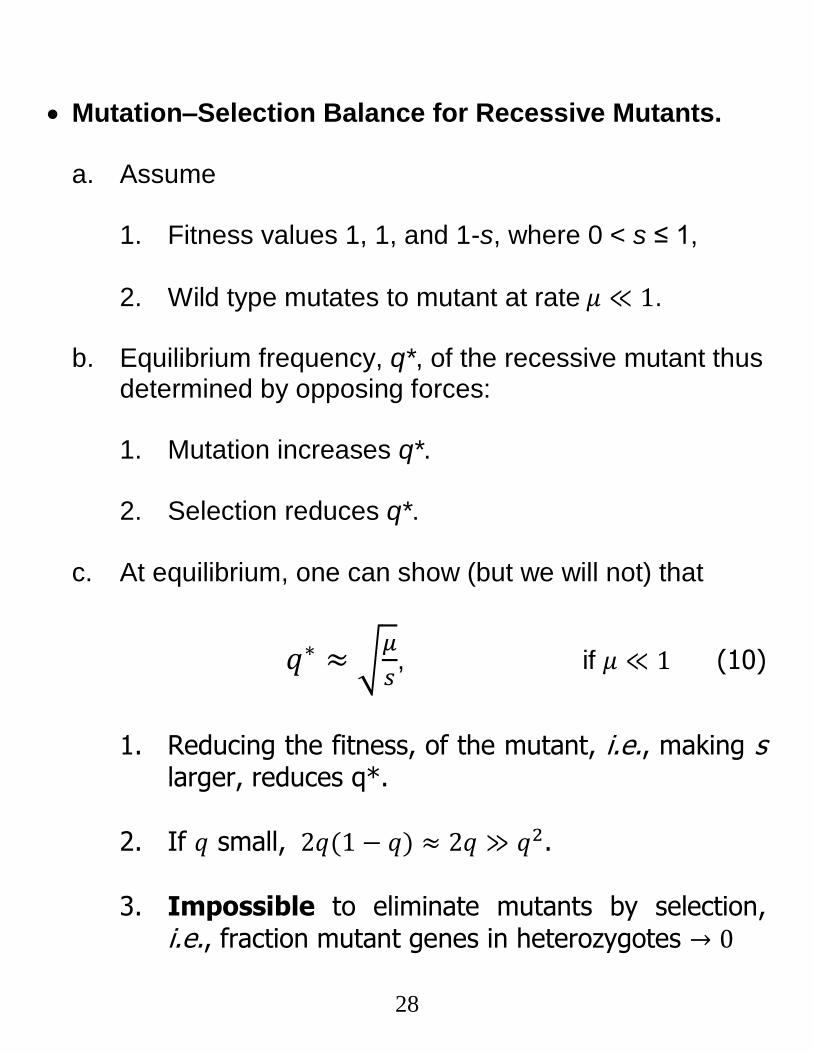
Mutation–Selection Balance for Recessive Mutants.

a. Assume

1. Fitness values 1, 1, and 1-s, where 0 < s ≤ 1,

2. Wild type mutates to mutant at rate 𝜇 ≪ 1.

b. Equilibrium frequency, q*, of the recessive mutant thus determined by opposing forces: 1. Mutation increases q*.

2. Selection reduces q*.

c. At equilibrium, one can show (but we will not) that

𝑞∗ ≈ √𝜇

𝑠, if 𝜇 ≪ 1 (10)

1. Reducing the fitness, of the mutant, i.e., making s

larger, reduces q*.

2. If 𝑞 small, 2𝑞(1 − 𝑞) ≈ 2𝑞 ≫ 𝑞2.

3. Impossible to eliminate mutants by selection,

i.e., fraction mutant genes in heterozygotes → 0

29

d. If the mutant is dominant, selection more effective

because both heterozygotes and homozygotes are exposed to selection and their numbers reduced.

e. Recessive mutations are more difficult to eliminate

than dominant mutations because only homozygotes are exposed to selection.

f. Important implications for animal breeding and human

eugenics.

g. Appreciated by 20th century eugenists who nonethe-less were enthusiastic in their advocacy for “racial hy-giene”.

Mutation – selection balance for recessive (top) and dominant (bottom) mutations. Equilibrial gene frequencies given by the in-

tersection of −∆𝒒𝒔𝒆𝒍 and ∆𝒒𝒎𝒖𝒕.

30

Question.

12. Tay-Sachs disease (TSD) occurs in frequencies of .03-.04 in Jews of Eastern European extraction. TSD is a neurodegenerative disorder caused by a single autoso-mal mutation. In its most common form, it is almost in-variably fatal by age 4. Assume the disease only pre-sents in homozygotes (two copies of the mutation) and a mutation rate of 2 X 10-6.

a. Compute the equilibrium frequency of TSD according

to Eq (10). Hint: What is the value of the coefficient of selection, s ?

b. What do you conclude?

31

Migration. a. Most species divided into local populations coupled by

migration. Consequence of 1. Inherent limitations to dispersal;

2. Geographic barriers.

b. Because conditions vary spatially, gene frequencies of-

ten vary along geographic transects 1. E.g., increasing body size in mammals as one goes

from equator to poles (Bergmann’s rule – next page).

2. Consequence of selection for larger body size in cold

climates. c. Gene flow (consequence of migration)

1. Retards local differentiation that would other-wise result from differing selective regimes.

2. Holds species together genetically, i.e., prevents

gene frequency divergence of local populations.

32

The range of white-tailed deer (Odocoileus virginianus) extends from Canada to the Amazon basin. There is a strong size gradient, with the largest animals in the north

(left) and the smallest in the tropics (right).

33

Part III. The “Stuff” of Evolution.

Quantitative Genetics.

a. Studies “continuous” variation.

1. Examples include size, crop yield, fat content in meat, IQ, blood pressure, bristle number in fruit flies. etc.

2. Reflects polygenic (many genes) control of most

quantitative traits. Recall Fisher’s reconciliation of Mendelism and Darwin-Wallace selection.

3. Quantitative traits typically under both environ-

mental and genetic control.

Distribution of a quantitative character in a population. Left. Raw data. Right. Continuous distribution inferred therefrom.

34

b. The Big Picture:

1. Both Mendelian and quantitative genetics are models of heredity.

2. Mendelian genetics focuses on allelic frequencies and phenotypically discrete genotypes;

3. Quantitative genetics focuses on distributions of

trait values that are more or less continuous.

Appropriate Genetic Model

Within Genotype Variability

Between Genotype Variability

Mendelian Small Large

Quantitative Large Small

35

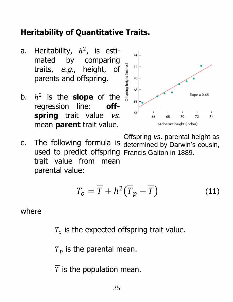
Heritability of Quantitative Traits.

a. Heritability, ℎ2, is esti-

mated by comparing traits, e.g., height, of parents and offspring.

b. ℎ2 is the slope of the

regression line: off-spring trait value vs. mean parent trait value.

c. The following formula is used to predict offspring trait value from mean parental value:

𝑇𝑜 = 𝑇 + ℎ2(𝑇𝑝 − 𝑇) (11)

where

𝑇𝑜 is the expected offspring trait value.

𝑇𝑝 is the parental mean.

𝑇 is the population mean.

Offspring vs. parental height as determined by Darwin’s cousin, Francis Galton in 1889.

36

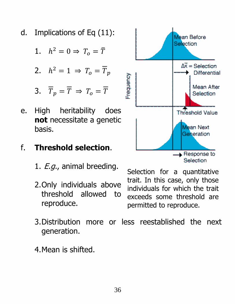
d. Implications of Eq (11):

1. ℎ2 = 0 ⇒ 𝑇𝑜 = �̅�

2. ℎ2 = 1 ⇒ 𝑇𝑜 = 𝑇𝑝

3. 𝑇𝑝 = 𝑇 ⇒ 𝑇𝑜 = 𝑇

e. High heritability does

not necessitate a genetic basis.

f. Threshold selection.

1. E.g., animal breeding.

2. Only individuals above

threshold allowed to reproduce.

3. Distribution more or less reestablished the next

generation.

4. Mean is shifted.

Selection for a quantitative trait. In this case, only those individuals for which the trait exceeds some threshold are permitted to reproduce.

37

Questions.

13. Parent-offspring comparisons in humans would yield high heritability for life-time earning and religion – i.e., the children of the rich tend to be rich, etc. Does this necessitate the existence of “poverty genes”? Explain.

14. In assessing whether or not intelligence has a heritable basis, twin studies are often used. Design such a study.

15. Assume the average IQ in a population is 100 and

ℎ 2 = 0.4. What is the expected IQ of the daughter of parents whose IQs are 120 and 110? What about the IQ of a child born to parents with IQs of 90?

16. Comparing the offspring’s expected IQ to that of the

parents and to the population mean, what do you conclude?

38

Types of Selection on Quantitative Characters.

Stabilizing (left), directional (center) and disruptive (right) se-lection. Blue arrows indicate phenotypes selected against.

39

Directional Selection in Cliff Swallows.

a. Mammals and birds maintain constant body temperature.

b. In cold enviroments, heat lost

to the environment must be balanced by heat generated metabolically.

c. Small individuals have a heat loss problem due to large surface area to volume ratios.

d. In the case of insectivorous

birds, cold weather further reduces food availability and therefore the rate at which heat can be generated.

e. Cold weather should select for larger body size.

f. Following a series of severe breeding season storms

(cold, rainy weather) in Nebraska, differential mortality was observed with small birds being more likely to wind up dead below the nests.

Cliff swallows are North American insectivorous birds that catch their food on the fly. They are also colonial nesters.

40

Foot length in dead (black) and surviving (shaded) cliff swallows following a cold-snap in Nebraska during the breeding season.

41

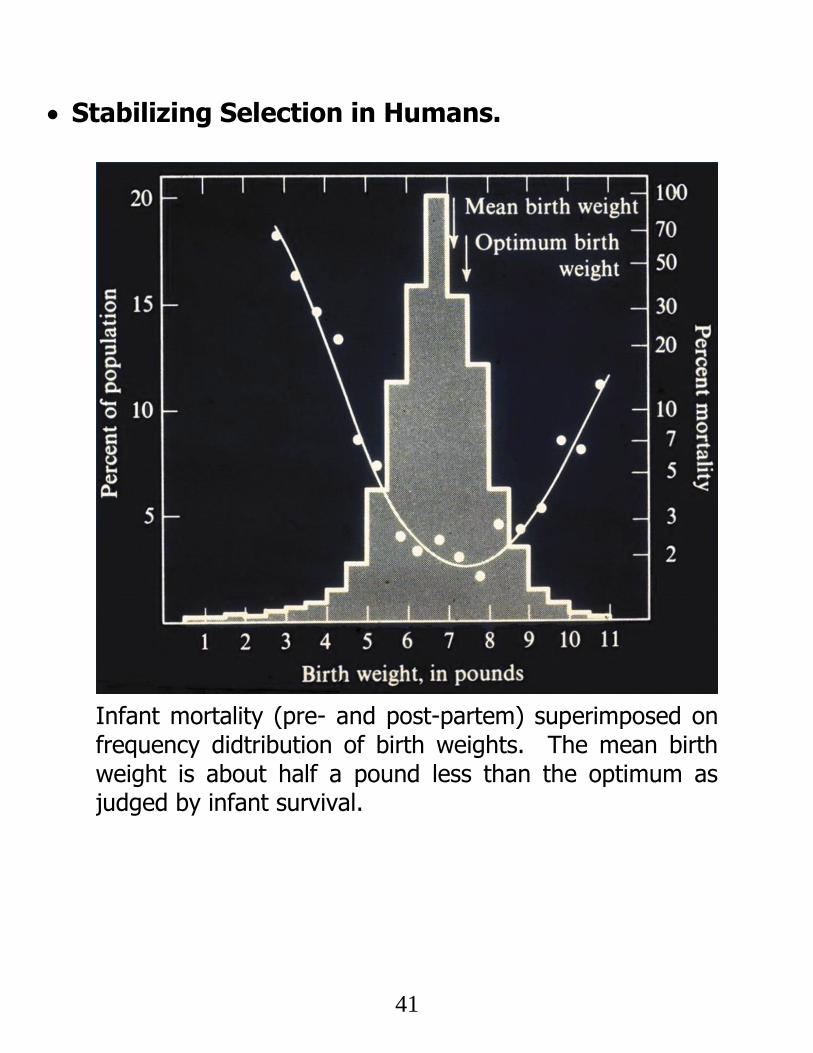
Stabilizing Selection in Humans.

Infant mortality (pre- and post-partem) superimposed on frequency didtribution of birth weights. The mean birth weight is about half a pound less than the optimum as judged by infant survival.

42

Disruptive Selection in Finches.

a. Selection for small and large bills in an African finch. (black bellied seed cracker)

b. Feed principally on seeds of

two species of grass-like plants (sedges) that live in wetlands.

1. Seeds about the same size. 2. Differ dramatically in hardness.

3. Smaller bills better for manipulating seeds but can’t

crack hard ones. 4. Larger bills better for cracking hard seeds.

c. Result is selection for small and large bills and against

bills of intermediate size. d. Supported by observation of differential juvenile survival

depending on bill size – see figure on next page.

Black bellied seed crack-ers. Only the male (right) has a black belly.

43

Selection for small and large bills in black bellied seed crackers. Light orange bars represent all juveniles; dark orange bars, those that survived to adulthood.

44

Questions.

17. Which of the three modes (stabilizing, directional, disruptive) of selection always increases phenotypic variance? Which mode shifts trait frequency distributions?

18. Which of the three modes of selection is often a

consequence of trade-offs and could be responsible for evolutionary stasis?

19. How might you account for the fact that the observed

mean birth weight of humans is slightly less than the optimum?

20. The following species nest in Alaska where summer

nights can be cold: golden eagle, great horned owl, kingbird, rufous hummingbird, yellow-shafted flicker. One of these goes torpid (reduced metabolic rate and body temperature) at night. Which species do you imagine does this? Explain.

21. Small cliff swallows are more agile fliers than large

individuals and therefore more likely to be able to capture insects on the fly. How does this affect selection for body size in this species?