everyone-a-banker or ideal credit acceptance game: theory and evidence
DESCRIPTION
Everyone-a-banker or Ideal Credit Acceptance Game: Theory and Evidence. Jürgen Huber, Martin Shubik and Shyam Sunder Waseda University, Tokyo, Japan, January 22, 2008. An Overview. Back ground paper (Three Minimal Market Institutions) - PowerPoint PPT PresentationTRANSCRIPT

Everyone-a-banker or Ideal Credit Acceptance Game: Theory
and EvidenceJürgen Huber, Martin Shubik and
Shyam SunderWaseda University, Tokyo,
Japan, January 22, 2008

An Overview• Back ground paper (Three Minimal Market Institutions)• Is personal credit issued by individuals sufficient to operate an
economy efficiently with no outside or government money?• Sorin (1995)’s construction of a strategic market game proves that it
is possible• We report on a laboratory experiment in which each agent issues
IOUs, and a costless efficient clearinghouse adjusts the exchange rates so markets always clear
• Results: when information system and clearinghouse preclude moral hazard, information asymmetry or need for trust, such economy operates efficiently without government money
• Conversely, it may be better to look for explanations for the prevalence of government money either in the abovementioned frictions, or in our unwillingness to experiment with innovation

Three Minimal Market Institutions: Theory and Experimental Evidence
(August 2007)
Jürgen Huber, University of Innsbruck
Martin Shubik, Yale University
Shyam Sunder, Yale University

Outline
• Three minimal market designs
• Experimental implementation
• Results compared to three benchmarks:– General equilibrium– Non-cooperative equilibrium with 10 traders– Zero-intelligence traders (simulation)
• Concluding remarks and research plans

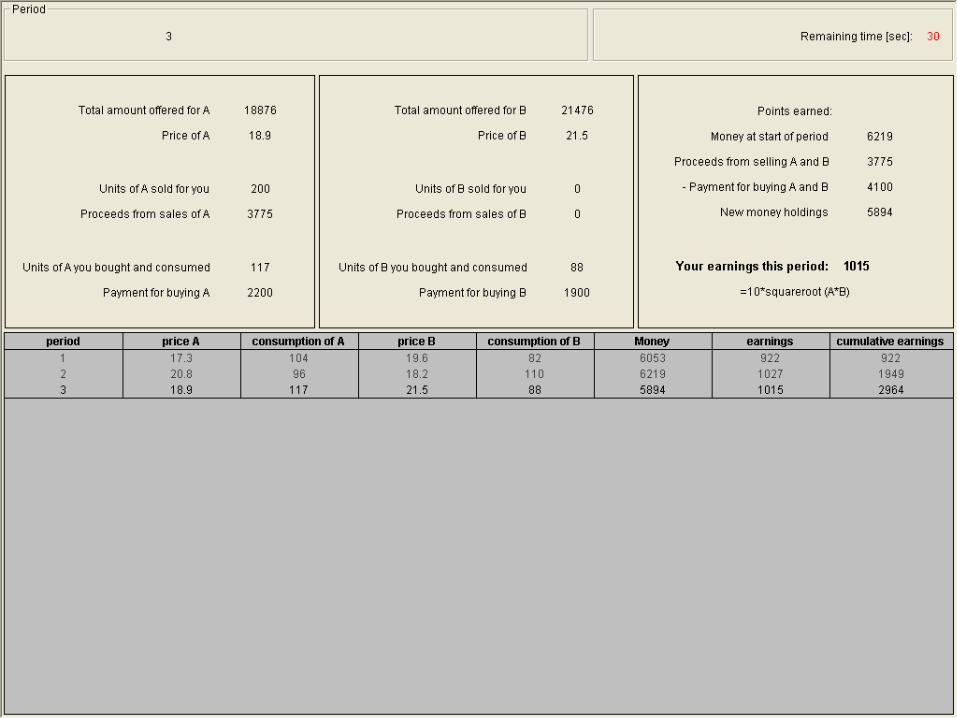
Market setup (in all three settings)
• Two goods (A and B) traded for money• Each trader endowed with either A or B and
money• Multiplicative earnings function:
Earnings = squareroot(A x B) + net money• Money carried over from period to period (except
in double auction)

Three Minimal Market Institutions
1. The sell-all model (strategy set dimension 1: all commodity endowment sold; each trader bids an amount of money to buy each commodity)
2. The buy-sell model (strategy set dimension 2: each trader offers the quantity of endowed good and bids money for the other good)
3. The simultaneous double auction model (strategy set dimension 4: each trader offers to sell each good and bids to buy each good)

Sell All Market

Buy-Sell Market


Double Auction

Endowments(Good A/Good B/Money)
• 200/0/6000 or 0/200/6000 in sell-all
• 200/0/4000 or 0/200/4000 in buy-sell
• 20/0/4000 or 0/20/4000 in double-auction
• 10 traders in each market (5+5)
• One buy-sell market with 20 traders (10+10)

Initial CGE
Quantity/
Price
NCE (5+5)
Quantity/
Price
A B A B A B
Sell All 200 0 100/20
100/ 20
110/20.1
90/
20.1
Buy Sell 200 0 100/20
100/ 20
122/20
78/ 20
Double Auction
20 0 10/ 100
10/ 100
11/ 100
9 100
General and Non-cooperative equilibria

Figure 1: Efficiency of Allocations (Average Earnings) for n = 5+5
Sell-All (Run 1, Mean=97.7) Sell-All (Run 2, Mean=97.6)
0
25
50
75
100
1 2 3 4 5 6 7 8 9 10 11 12 13 14 15 16 17 18 19 20
Period
0
25
50
75
100
1 2 3 4 5 6 7 8 9 10 11 12 13 14 15 16 17 18 19 20
Period
Buy-Sell (Run 3, Mean=91.4) Buy-Sell (Run 4, Mean=94.6)
0
25
50
75
100
1 2 3 4 5 6 7 8 9 10 11 12 13 14 15 16 17 18 19 20
Period
0
25
50
75
100
1 2 3 4 5 6 7 8 9 10 11 12 13 14 15 16 17 18 19 20
Period
Double Auction (Run 5, Mean=87.8) Double Auction (Run 6, Mean=93.2)
0
25
50
75
100
1 2 3 4 5 6 7 8 9 10
Period
0
25
50
75
100
1 2 3 4 5 6 7 8 9 1 11
Period
Figure 1: Efficiency of Allocations (Average Earnings)
for n = 5+5

Figure 2: Performance of Buy-Sell Market
with n = 10 + 10 Earnings (Mean=98.1) Prices (Mean=16.4 for A, 16.5 for B)
0
25
50
75
100
1 2 3 4 5 6 7 8 9 10 11 12 13 14 15 16 17 18 19 20
Period
0
10
20
30
40
1 2 3 4 5 6 7 8 9 10 11 12 13 14 15 16 17 18 19 20
Period
Symmetry (Mean=0.81) Unspent money (Mean=62.45 percent)
0.00
0.25
0.50
0.75
1.00
1 2 3 4 5 6 7 8 9 10 11 12 13 14 15 16 17 18 19 20
Period
0
25
50
75
100
1 2 3 4 5 6 7 8 9 10 11 12 13 14 15 16 17 18 19 20
Period
Standard dev. Of Earnings (Mean=118) Trade as % of trade needed to achieve GE
0
250
500
750
1 2 3 4 5 6 7 8 9 10 11 12 13 14 15 16 17 18 19 20
Period
0
25
50
75
100
125
1 2 3 4 5 6 7 8 9 10 11 12 13 14 15 16 17 18 19 20
Period

Figure 3: Price Levels and Developments for n = 5+5
Sell-All (Run 1, Avg. A=18.92; B=20.90) Sell-All (Run 2, Avg. A=21.52; B=20.49)
0
10
20
30
40
1 2 3 4 5 6 7 8 9 10 11 12 13 14 15 16 17 18 19 20
Period
0
10
20
30
40
1 2 3 4 5 6 7 8 9 10 11 12 13 14 15 16 17 18 19 20
Period
Buy-Sell (Run 3, Avg. A=11.32; B=9.24) Buy-Sell (Run 4, Avg.A=19.89; B=16.34)
0
10
20
30
40
1 2 3 4 5 6 7 8 9 10 11 12 13 14 15 16 17 18 19 20
Period
0
10
20
30
40
1 2 3 4 5 6 7 8 9 10 11 12 13 14 15 16 17 18 19 20
Period
Double Auction (Run 5, Avg. A=261; B=246) Double Auction (Run 6, Avg. A=225; B=170)
0
100
200
300
400
1 2 3 4 5 6 7 8 9 10
Period
0
100
200
300
400
1 2 3 4 5 6 7 8 9 1 11
Period

Figure 4: Double Auction Transaction Price Paths within individual Trading Periods with G-S traders
0
10
20
30
40
50
60
70
80
90
100
1 4 7 10 13 16 19 22 25 28 31 34 37 40 43 46 49 52
Run 5: Transaction Sequence No.
Pri
ce
s
Series1
Series2
Series3
Series4
Series5
Series6
Series7
Series8
Series9
Series10
Series11
0
10
20
30
40
50
60
70
80
90
100
1 4 7 10 13 16 19 22 25 28 31 34 37 40 43 46 49 52
Run 6: Transaction Sequence No.
Pri
ce
s
Series1
Series2
Series3
Series4
Series5
Series6
Series7
Series8
Series9
Series10
Series11

Figure 5: Symmetry of Allocations
for n = 5+5 Sell-All (Session 1, Mean=0.76) Sell-All (Session 2, Mean=0.71)
0.00
0.25
0.50
0.75
1.00
1 2 3 4 5 6 7 8 9 10 11 12 13 14 15 16 17 18 19 20
Period
0.00
0.25
0.50
0.75
1.00
1 2 3 4 5 6 7 8 9 10 11 12 13 14 15 16 17 18 19 20
Period
Buy-Sell (Session 3, Mean=0.60) Buy-Sell (Session 4, Mean=0.71)
0.00
0.25
0.50
0.75
1.00
1 2 3 4 5 6 7 8 9 10 11 12 13 14 15 16 17 18 19 20
Period
0.00
0.25
0.50
0.75
1.00
1 2 3 4 5 6 7 8 9 10 11 12 13 14 15 16 17 18 19 20
Period
Double Auction (Session 5, Mean=0.53) Double Auction (Session 6, Mean=0.60)
0.00
0.25
0.50
0.75
1.00
1 2 3 4 5 6 7 8 9 10
Period
0.00
0.25
0.50
0.75
1.00
1 2 3 4 5 6 7 8 9 1 11
Period
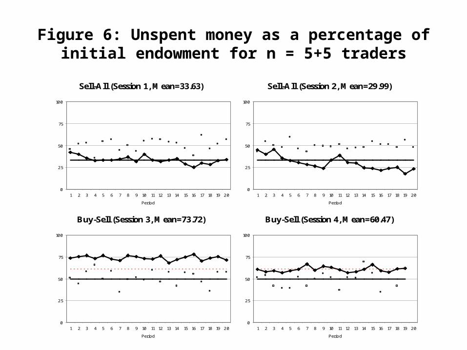
Figure 6: Unspent money as a percentage of initial endowment for n = 5+5 traders
Sell-All (Session 1, Mean=33.63) Sell-All (Session 2, Mean=29.99)
0
25
50
75
100
1 2 3 4 5 6 7 8 9 10 11 12 13 14 15 16 17 18 19 20
Period
0
25
50
75
100
1 2 3 4 5 6 7 8 9 10 11 12 13 14 15 16 17 18 19 20
Period
Buy-Sell (Session 3, Mean=73.72) Buy-Sell (Session 4, Mean=60.47)
0
25
50
75
100
1 2 3 4 5 6 7 8 9 10 11 12 13 14 15 16 17 18 19 20
Period
0
25
50
75
100
1 2 3 4 5 6 7 8 9 10 11 12 13 14 15 16 17 18 19 20
Period

Figure 7: Standard Deviation of Earnings per Period Sell-All (Session 1, Mean=150) Sell-All (Session 2, Mean=165)
0
250
500
750
1 2 3 4 5 6 7 8 9 10 11 12 13 14 15 16 17 18 19 20
Period
0
250
500
750
1 2 3 4 5 6 7 8 9 10 11 12 13 14 15 16 17 18 19 20
Period
Buy-Sell (Session 3, Mean=463) Buy-Sell (Session 4, Mean=243)
0
250
500
750
1 2 3 4 5 6 7 8 9 10 11 12 13 14 15 16 17 18 19 20
Period
0
250
500
750
1 2 3 4 5 6 7 8 9 10 11 12 13 14 15 16 17 18 19 20
Period
Double Auction (Session 5, Mean=261) Double Auction (Session 6, Mean=362)
0
250
500
750
1 2 3 4 5 6 7 8 9 10
Period
0
250
500
750
1 2 3 4 5 6 7 8 9 1 11
Period

Figure 8: Goods traded as Percentage of Trade needed
to achieve GE Sell-All (Session 1, Mean=86.63) Sell-All (Session 2, Mean=82.97)
0
25
50
75
100
125
1 2 3 4 5 6 7 8 9 10 11 12 13 14 15 16 17 18 19 20
Period
0
25
50
75
100
125
1 2 3 4 5 6 7 8 9 10 11 12 13 14 15 16 17 18 19 20
Period
Buy-Sell (Session 3, Mean=105.16) Buy-Sell (Session 4, Mean=88.75)
0
25
50
75
100
125
1 2 3 4 5 6 7 8 9 10 11 12 13 14 15 16 17 18 19 20
Period
0
25
50
75
100
125
1 2 3 4 5 6 7 8 9 10 11 12 13 14 15 16 17 18 19 20
Period
Double Auction (Session 5, Mean=68.40) Double Auction (Session 6, Mean=80.91)
0
25
50
75
100
125
1 2 3 4 5 6 7 8 9 10
Period
0
25
50
75
100
125
1 2 3 4 5 6 7 8 9 1 11
Period
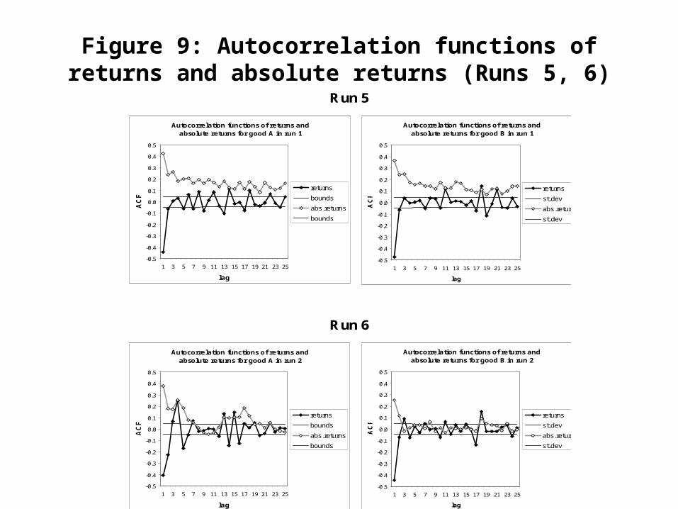
Figure 9: Autocorrelation functions of returns and absolute returns (Runs 5, 6)
Autocorrelation functions of returns and absolute returns for good A in run 1
-0.5
-0.4
-0.3
-0.2
-0.1
0.0
0.1
0.2
0.3
0.4
0.5
1 3 5 7 9 11 13 15 17 19 21 23 25
lag
AC
F
returns
bounds
abs.returns
bounds
Autocorrelation functions of returns and absolute returns for good A in run 2
-0.5
-0.4
-0.3
-0.2
-0.1
0.0
0.1
0.2
0.3
0.4
0.5
1 3 5 7 9 11 13 15 17 19 21 23 25
lag
AC
F
returns
bounds
abs.returns
bounds
Run 5
Autocorrelation functions of returns and absolute returns for good B in run 1
-0.5
-0.4
-0.3
-0.2
-0.1
0.0
0.1
0.2
0.3
0.4
0.5
1 3 5 7 9 11 13 15 17 19 21 23 25
lag
AC
F
returns
st.dev
abs.returns
st.dev
Run 6
Autocorrelation functions of returns and absolute returns for good B in run 2
-0.5
-0.4
-0.3
-0.2
-0.1
0.0
0.1
0.2
0.3
0.4
0.5
1 3 5 7 9 11 13 15 17 19 21 23 25
lag
AC
F
returns
st.dev
abs.returns
st.dev

Comparison of markets I
Avg. Earnings as percentage of maximum
86%
88%
90%
92%
94%
96%
98%
100%
Sell all Buy sell Double auction
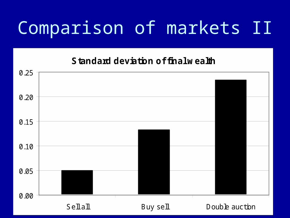
Comparison of markets II
Standard deviation of final wealth
0.00
0.05
0.10
0.15
0.20
0.25
Sell all Buy sell Double auction

SymmetryBuy-sell
Sell-all
Double auction
0.00
0.25
0.50
0.75
1.00
1 2 3 4 5 6 7 8 9 10 11 12 13 14 15 16 17 18 19 20
Period
0.00
0.25
0.50
0.75
1.00
1 2 3 4 5 6 7 8 9 10 11 12 13 14 15 16 17 18 19 20
Period
0.00
0.25
0.50
0.75
1.00
1 2 3 4 5 6 7 8 9 10
Period

Comparison of markets III'Symmetry' of Investment in different Treatments
0.00
0.20
0.40
0.60
0.80
1.00
Sell All Buy-Sell Double Auction
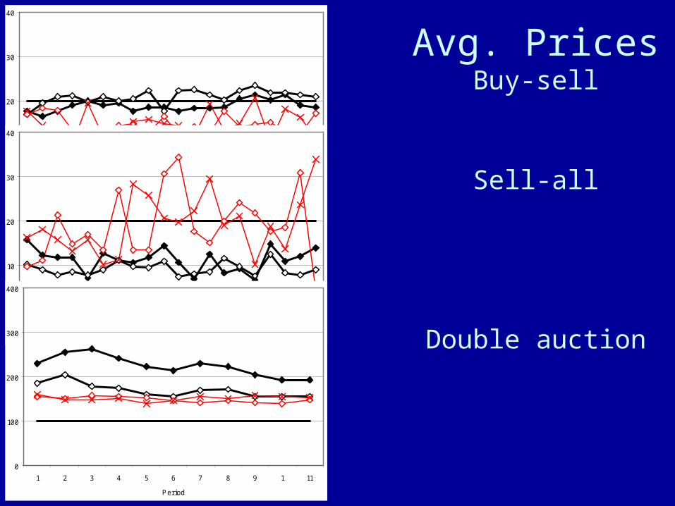
Avg. PricesBuy-sell
Sell-all
Double auction
0
10
20
30
40
1 2 3 4 5 6 7 8 9 10 11 12 13 14 15 16 17 18 19 20
Period
0
10
20
30
40
1 2 3 4 5 6 7 8 9 10 11 12 13 14 15 16 17 18 19 20
Period
0
100
200
300
400
1 2 3 4 5 6 7 8 9 1 11
Period

Trading vol.Buy-sell
Sell-all
Double auction
0
25
50
75
100
125
1 2 3 4 5 6 7 8 9 10 11 12 13 14 15 16 17 18 19 20
Period
0
25
50
75
100
125
1 2 3 4 5 6 7 8 9 10 11 12 13 14 15 16 17 18 19 20
Period
0
25
50
75
100
125
1 2 3 4 5 6 7 8 9 1 11
Period

Conclusions from the Background Paper
• The non-cooperative and general competitive equilibrium models provide a reasonable anchor to locate the observed outcomes of the three market mechanisms
• Unlike well known results from many partial equilibrium double auctions, prices and allocations in our double auctions reveal significant and persistent deviations from CGE predictions
• The market form has a significant influence on allocative efficiency and the return distribution: the outcome paths from the three market mechanisms exhibit significant differences among them.

The Current Paper:Need for Government Money?
• Is outside or government money necessary to operate an economy efficiently?
• Proponents of alternatives to government money suggest that if all individuals and institutions could issue debt as means of payment, market will sort out the risk and reputations of accepting such paper;
• For example, Black (1970); rates of interest in the City of London for “prime” and “lesser” names, discounting of bills issued by hundreds of banks in the free banking era of the U.S.

Strategic Market Game
• Outside or government money is not needed if the is perfect clearing and no default
• Result is valid under conditions which are clearly counterfactual (like M&M on neutrality of cost of capital with respect to leverage)
• Logical possibility of such an economy does not mean that an economy will actually function smoothly with private money under exogenous uncertainty, and dispersed and imperfect information
• Process dynamics, trust and evaluation are core issues in functioning of a financial system and are absence in Black or M&M equilibrium models

Acceptability of Government Money
• No bank (much less individual) can match the visibility of government,
• Government’s reputation is known to all• Government is better able to enforce the rules of the game• Government money expedited and simplified taxation as an
unintended (?) consequence• Handed to government additional policy options (e.g., financing of
wars and control of economy)• Acceptability of IOUs involves trust and trust in government may be
higher in most instances than in even big banks (individuals have little chance)
• Everyone-a-banker game could be seen as a simplified version of governments issuing their own money in the international exchanges to settle their payments
• In the experiment presented here, we cleanse the lab economy of such frictional and informational issues to ask if the logical possibility of private money economy is also a behavioral possibility
Laboratory Modeling• Computer implements the sell-all model• Uses the quantities endowed and money bid for each good to
calculate a market clearing price for each good and exchange rates for each trader’s money
• Computer acts as a clearing house as well as a perfect reputation enforcement mechanism (no reneging, no bankruptcy)
• Examines every-one-a-banker model in absence of uncertainty-related explanations for government money
• Yields high efficiencies• Key theoretical claim that government money is not needed for
efficiency exchanges is supported experimentally under these circumstances– Ideal contract enforcement, credit evaluation, and clearing
arrangements

Sorin (1995) Model
., Iibtqp iii
Consider a set A of n agents and set I of m goods. There are m posts, one for each good where each agent α bids quantity of money bi α for good i and offers a quantity of goods qi α of good i for sale. The equations defining prices in terms of the unit of account with tare:
And the budget balance gives
., Apqbt iiii
i
Equilibrium
• Sorin establishes the existence of an active non-cooperative equilibrium set of prices and exchange rates which converges to a competitive equilibrium as the number of traders increases
• The clearinghouse balances expenditures and revenues for all.

Experiment
• Two goods• Two types of traders with endowment (200,0) and (0,
200)• Upper limit on IOU (6,000)• Each agent submits bids for each good each period
subject to total < 6,000• Computer calculates the prices of two goods in each
personal currency and allocates goods• Points earned = squareroot (CA* CB)• CE: 2000 units to get 100 units of each good• With 5+5 agents, bid 2214+1811 for the two goods

Table 1: Non-cooperative Equilibria in the sell-all model
Players on each side
Money bid for
owned
good
Money bid for
other good
Bid owned/bid other
Sum of bids Money unspent
Price Units of owne
d good boug
ht
Units of other good boug
ht
Allocative Efficienc
y
2 2653.51 1573.72 1.6861 4227.23 1772.77 21.14 125.54 74.46 96.68
3 2382.02 1698.17 1.4027 4080.19 1919.81 20.40 116.76 83.24 98.59
4 2273.52 1767.29 1.2864 4040.81 1959.20 20.20 112.53 87.47 99.21
5* 2213.79 1810.88 1.2225 4024.67 1975.33 20.12 110.01 89.99 99.50
6 2175.72 1840.80 1.1819 4016.52 1983.48 20.08 108.34 91.66 99.65
7 2149.25 1862.58 1.1539 4011.83 1988.17 20.06 107.15 92.85 99.74
8 2129.75 1879.13 1.1334 4008.88 1991.12 20.04 106.25 93.75 99.80
9 2114.78 1892.14 1.1177 4006.92 1993.08 20.03 105.56 94.44 99.85
10 2102.92 1902.62 1.1053 4005.54 1994.46 20.03 105.00 95.00 99.87
many 2000.00 2000.00 1.0000 4000.00 2000.00 20.00 100.00 100.00 100.00
*Number of subject pairs in the laboratory experiment.Money endowment (M) = 6,000 units per traderGoods endowment = (200,0) for one member and (0,200) for the member of each pair of traders.

Allocation of Money
• Fig. 1: Money spending balanced between goods A and B
• CGE predicts equal amount spent on two goods• With 5+5 subjects, non-cooperative equilibrium
predicts 22 percent more money being spent to the owned good
• Table 2 and Figure 2 data are weakly consistent with this prediction
• The results appear to be closer to CE than to non-cooperative equilibrium

Figure 1: Investment into good A as a Percentage of Total Investment
Percentage of Total Investment invested into Good A over Time
0%
10%
20%
30%
40%
50%
60%
1 2 3 4 5 6 7 8 9 10 11 12 13 14 15
Period
Inve
stm
ent
in G
oo
d A T1, run 1
T1, run 2
T1, run 3
T2, run 1
T2, run 2
Avg.

Table 2: Percentage of total spending invested in A and B
(Separated by those endowed with the proceeds from selling A and those endowed with the proceeds from selling B)
Spending for A by A-holders
Spending for A by B-holders
Spending for B by A-holders
Spending for B by B-holders
Own-good-bias*
own-good-bias (as %age of other good)**
T1, run 1 54.6% 46.0% 45.4% 54.0% 8.6% 18.9%
T1, run 2 49.3% 49.3% 50.7% 50.7% 0.0% 0.0%
T1, run 3 50.8% 49.5% 49.2% 50.5% 1.3% 2.7%
T2, run 1 51.6% 47.0% 48.4% 53.0% 4.5% 9.9%
T2, run 2 52.3% 50.4% 47.7% 49.6% 1.9% 4.2%
*Own-good-bias: the percentage spent for the own good minus the percentage spend for the other good. **The final column presents this bias as percentage of the spending for the other good

Figure 2: Investment in good A as a Percentage of Total Investment separately for A-holders and B-holders (Averaged
Across Five Sessions) Investment in Good A Seperately for A-Holders and B-Holders
0%
10%
20%
30%
40%
50%
60%
1 2 3 4 5 6 7 8 9 10 11 12 13 14 15
Period
Pe
rce
nta
ge
of
Mo
ne
y s
pe
nt
for
A
A holders in A
B holders in A

Symmetry of Investment
• Smaller investment /larger investment in the two goods
• 0-1
• Period-wise averages charted in Figure 3
• Symmetry ranges from .7 to .95, slightly higher than the average of .65 in HSS 2007

Figure 3: Average ‘symmetry’ of investment in
the different experimental runs
Average 'symmetry' of investment
0.00
0.20
0.40
0.60
0.80
1.00
1 2 3 4 5 6 7 8 9 10 11 12 13 14 15
period
T1, run 1T1, run 2T1, run 3T2, run 1T2, run 2ZERO

Allocative Efficiency
• Actual number of points earned/Maximum possible points (i.e. CGE)
• Observations in range 96.9 to 99.3 (Figure 4)• Most traders invested equal amounts in the two
goods• Session 1 has lowest symmetry and efficiency• With efficient decisions from the beginning, little
opportunity to “learn” over time• Low cross sectional dispersion of earnings

Figure 4: Average points earned in the different
experimental runs Average points earned
60
70
80
90
100
1 2 3 4 5 6 7 8 9 10 11 12 13 14 15
period
mo
ne
y p
rin
ted
T1, run 1
T1, run 2
T1, run 3
T2, run 1
T2, run 2
ZERO

Credit Limit Actually Used
• Varied widely over range 30-90 percent (Figure 5)
• Little stability
• Suggest continuum of non-cooperative equilibria
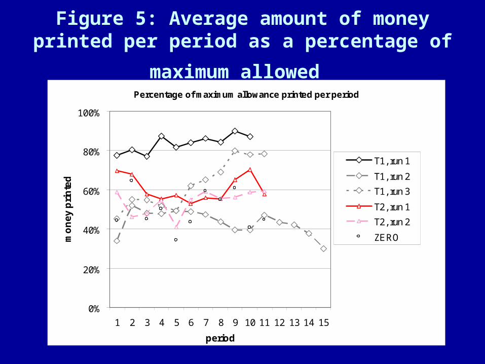
Figure 5: Average amount of money printed per
period as a percentage of maximum allowed Percentage of maximum allowance printed per period
0%
20%
40%
60%
80%
100%
1 2 3 4 5 6 7 8 9 10 11 12 13 14 15
period
mo
ne
y p
rin
ted
T1, run 1
T1, run 2
T1, run 3
T2, run 1
T2, run 2
ZERO

Link Between Money Printed (Percent of Credit Limit Used) and
Earnings of Individuals• No detectable link
• The economy offers no advantage to those who print more
• Also, no disadvantage to those who print less
• The clearinghouse mechanism adjusts the exchange rates among money issued by various players appropriately
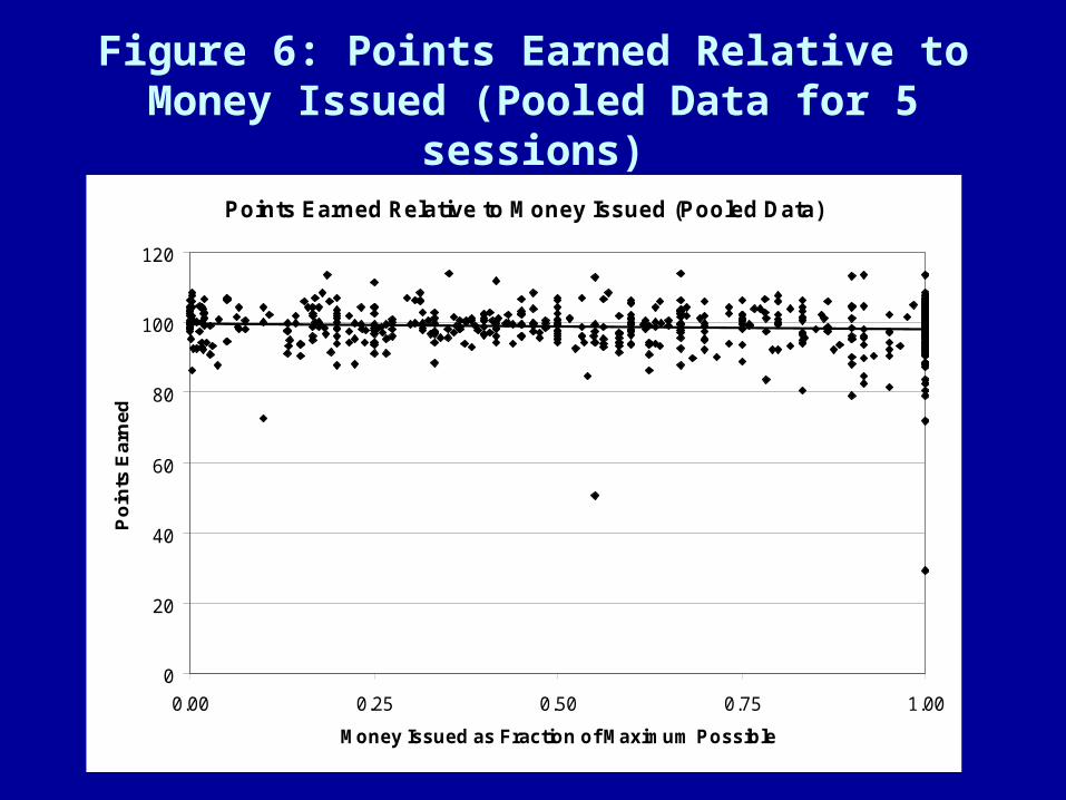
Figure 6: Points Earned Relative to Money Issued (Pooled Data for 5 sessions)
Points Earned Relative to Money Issued (Pooled Data)
0
20
40
60
80
100
120
0.00 0.25 0.50 0.75 1.00
Money Issued as Fraction of Maximum Possible
Po
ints
Ea
rne
d

Minimally Intelligent Agents
• Total spending ~U(0,6,000); split randomly between Goods A and B
• Efficiency 79% (4/5th of the gain from autarky to CGE from random behavior)
• Average spending 3000
• Average symmetry 0.39– Humans with symmetric behavior (0.80)
almost 100% efficient

Conclusions
• Theoretical analyses of strategic market games indicate that economy can approximate competitive outcomes with individually issued credit lines alone (without fiat or commodity money)
• This model abstracts away from transactions costs, intertemporal credit, possibility of default (forcing all traders to have perfect reputation for trusworthiness) through a perfect clearinghouse mechanism for enforcement (no accounting problems of intertemporal trade)
• The lab economy mimics these conditions postulated in the model economy (and tells us little about what would happen when these conditions are violated)

Conclusions
• This powerful market mechanism and clearinghouse puts enough structure to prevent non-correlated or at best weakly correlated behavior at a mass scale to go far wrong
• With small size of strategy sets, even economies populated with minimally intelligent agents perform reasonably well
• With more complex evaluative tasks, expertise may exhibit more value
• Design of future experiments with roles for reputation and expertise (e.g., non-delivery)– Social context problem in laboratory

Conclusions
• In the meantime, results reveal considerable power of market structure in producing efficient outcomes when reputation is not an issue
• Under such circumstances, the claim that government money is not needed for efficient exchange is supported analytically as well as experientially
• Future experiments under weaker conditions• In the free banking era in the U.S., different bank
notes sold at different discount rates depending on their individual reputation and acceptability

Points Earned When You Consume Varying Amounts of Goods A and B
Units of good B you buy and consume
Units of A you buy and con-sume
0 25 50 75 100 125 150 175 200 225 250
0 0 0 0 0 0 0 0 0 0 0 0
25 0 25 35 43 50 56 61 66 71 75 79
50 0 35 50 61 71 79 87 94 100 106 119
75 0 43 61 75 87 97 106 115 123 130 137
100 0 50 71 87 100 119 123 132 141 150 158
125 0 56 79 97 119 125 137 148 158 168 177
150 0 61 87 106 123 137 150 162 173 184 194
175 0 66 94 115 132 148 162 175 187 198 209
200 0 71 100 123 141 158 173 187 200 212 224
225 0 75 106 130 150 168 184 198 212 225 237
250 0 79 112 137 158 177 194 209 224 237 250


