Event-Triggered Attitude Stabilization ofa Quadcopter

DIOGO ALMEIDA

Master’s Degree ProjectStockholm, Sweden 2014

XR-EE-RT 2014:011

Abstract

There are many possible ways to perform the attitude control of a quad-copter and, recently, the subject of event-triggered control has becomerelevant in the scientific community. This thesis deals with the analysis andimplementation of a saturating attitude controller for a quadcopter system,together with the derivation of an event-triggering rule to work with it. Twodistinct rules are presented, one that ensures the stability of the closed loopsystem, the other, a linearised version that does not. The way those werederived consists in the use of a Lyapunov based approach. The stability ofthe system when under these rules was verified experimentally.

Keywords: Non-linear control; Attitude stabilization; Event-triggering;Quadcopter

i

To my mother

ii

Acknowledgements

I would like to thank all the friends that supported me during my studyyears, that culminated with this report, as well as my family for the constantsupport and encouragement.

Thanks to Dimos Dimarogonas for the supervision and for the suggestionsmade during the course of the project.

Special thanks to my friends at the Smart Mobility Lab for all the helpin setting up the experiments and for the well spent moments. They areFrancisco Martucci, Joao Pedro and Matteo Vanin.

iii

Contents

1 Introduction 11.1 Rigid-body attitude control . . . . . . . . . . . . . . . . . . . 1

1.1.1 Quadcopters . . . . . . . . . . . . . . . . . . . . . . . . 11.2 Event-Triggering Framework . . . . . . . . . . . . . . . . . . . 21.3 Objectives . . . . . . . . . . . . . . . . . . . . . . . . . . . . . 31.4 Thesis Outline . . . . . . . . . . . . . . . . . . . . . . . . . . . 3

2 Background 52.1 The quaternions . . . . . . . . . . . . . . . . . . . . . . . . . . 5

2.1.1 Operations with quaternions . . . . . . . . . . . . . . . 62.1.2 Quaternion of rotation . . . . . . . . . . . . . . . . . . 6

2.2 Quadcopter attitude control . . . . . . . . . . . . . . . . . . . 72.2.1 Attitude dynamics . . . . . . . . . . . . . . . . . . . . 82.2.2 Control approaches . . . . . . . . . . . . . . . . . . . . 112.2.3 Proposed controller . . . . . . . . . . . . . . . . . . . . 11

2.3 Event-Triggered control . . . . . . . . . . . . . . . . . . . . . . 15

3 Event-Triggering Rule 183.1 Problem statement . . . . . . . . . . . . . . . . . . . . . . . . 183.2 Rule derivation . . . . . . . . . . . . . . . . . . . . . . . . . . 193.3 Simulation results . . . . . . . . . . . . . . . . . . . . . . . . . 22

3.3.1 Triggering results . . . . . . . . . . . . . . . . . . . . . 24

4 Implementation 274.1 The hardware . . . . . . . . . . . . . . . . . . . . . . . . . . . 274.2 Firmware . . . . . . . . . . . . . . . . . . . . . . . . . . . . . 284.3 Motor thrust and inertia moments . . . . . . . . . . . . . . . . 294.4 Test stand . . . . . . . . . . . . . . . . . . . . . . . . . . . . . 33

5 Results 345.1 Time-triggered results . . . . . . . . . . . . . . . . . . . . . . 35

iv

5.2 Event-triggered results . . . . . . . . . . . . . . . . . . . . . . 36

6 Conclusions 386.1 Future work . . . . . . . . . . . . . . . . . . . . . . . . . . . . 38

A Linearised triggering rule derivation 40

B Experimental results 44

v

Chapter 1

Introduction

In recent years, the topic of event-triggered control has been subject of in-terest by the part of the research community. Several different triggeringstrategies have been developed and implemented with encouraging results,allowing for the reduction of the number of computations required for thesuccessful execution of control algorithms. In this thesis, a saturating atti-tude controller for a quadcopter is studied and implemented in a real system,and a triggering rule to work with it is derived.

1.1 Rigid-body attitude control

The subject of attitude control of a rigid-body is a well-known problem,that consists in sending the right command signals to a rigid-body system tomake it adopt a desired orientation, see figure 1.1. It is a tractable problem,with well known kinematics and dynamics equations, with several admissiblestabilizing control laws [4] [22].

A quadcopter helicopter can be thought of as a rigid body system, withthe same six degrees of freedom and under-actuated dynamics ([15] [10], forexample). This allows the application of known rigid-body control techniquesto this kind of systems, or to help in the development of new ones.

1.1.1 Quadcopters

The concept of a quadcopter is not new. The first reported working systemwas developed in 1907 [36], and one of the most successful designs for earlyhelicopter vehicles had precisely a quadcopter-like design [37]. It consists ona set of four arms making a cross shape, with rotors on each end. It is under-actuated, since it has six degrees of freedom (three spatial coordinates plus

1

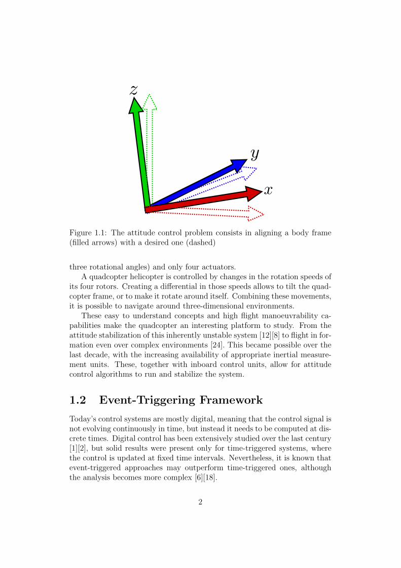
Figure 1.1: The attitude control problem consists in aligning a body frame(filled arrows) with a desired one (dashed)

three rotational angles) and only four actuators.A quadcopter helicopter is controlled by changes in the rotation speeds of

its four rotors. Creating a differential in those speeds allows to tilt the quad-copter frame, or to make it rotate around itself. Combining these movements,it is possible to navigate around three-dimensional environments.

These easy to understand concepts and high flight manoeuvrability ca-pabilities make the quadcopter an interesting platform to study. From theattitude stabilization of this inherently unstable system [12][8] to flight in for-mation even over complex environments [24]. This became possible over thelast decade, with the increasing availability of appropriate inertial measure-ment units. These, together with inboard control units, allow for attitudecontrol algorithms to run and stabilize the system.

1.2 Event-Triggering Framework

Today’s control systems are mostly digital, meaning that the control signal isnot evolving continuously in time, but instead it needs to be computed at dis-crete times. Digital control has been extensively studied over the last century[1][2], but solid results were present only for time-triggered systems, wherethe control is updated at fixed time intervals. Nevertheless, it is known thatevent-triggered approaches may outperform time-triggered ones, althoughthe analysis becomes more complex [6][18].

2

Event-triggered control is a control technique where the control signalsare computed only at instants where the plant is considered to need attention.Usually, an event-triggered system has three main components, the controller,an event generator and the network fabric, an abstraction of the network thatlinks the state sensing to the controller. Every time a measure of the plantstate fulfils a certain condition, the event generator feeds back the state tothe controller, that generates a new control signal. In between these instants,the signal may be kept constant or follow some kind of interpolating function[18].

The main purpose of this framework is to save network resources. Thismay mean that more bandwidth will be available for other tasks that sharethe network with the controller or that CPU usage can be minimized, andmostly allows for the development of control systems that operate in a re-source aware manner. While the reduction of the number of computationsis often the stated goal when developing this kind of systems, they can alsoshorten the inter-sampling time when the system requires so. This can bean advantage over the classical approach to digital control.

Some results for event-triggering control of dynamical systems have beenderived in recent years, where the event-triggering and feedback rule arederived from a Control Lyapunov Function [23][27], while others create anevent-triggering rule after defining the controller [25][17].

1.3 Objectives

In this thesis, the Fast and Saturating Attitude controller [28] is discussed,and an event-triggering rule to work with it is derived. Both the controllerand the triggering rule are then implemented on a real APM:Copter [33]system, where the stabilizing properties can be verified. The triggering ruleis compared with an heuristic approach, both in simulation and practicalsettings.

1.4 Thesis Outline

This report is organized as follows:

• In chapter 2, the necessary background for the project is given. Thisincludes quaternion based attitude parametrization, a discussion of theproposed saturating controller and an introduction to event-triggering;

• Chapter 3 presents the event-triggering rule derivation, the main con-tribution of the thesis. Two rules are proposed, one providing analyti-

3

cal stability guaranties, the other offering a simplification that reducessignificantly the computations that need to be carried out in betweensampling times. Both are compared with an heuristic error-based rule;

• Chapter 4 describes the implementation of the attitude control systemin a real quadcopter, together with an analysis of the results obtained;

• Finally, in chapter 6, conclusions and a discussion for future work arepresented.

4

Chapter 2

Background

For the discussion of the studied controller, a quaternion parametrizationof the attitude of a rigid body is used. The basics required to understandthat are presented in this chapter, together with the principles of working ofthe attitude controller. Finally, an introduction to event-triggered control isgiven. During the remaining of the text, all the norms ‖.‖ are the L2 normof a vector.

2.1 The quaternions

A quaternion is a mathematical object, originally aimed at expanding theset of the complex numbers, C, into three dimensional space. This newsystem would then add a second imaginary number, j, to an existing complexnumber, such that j2 = −1. The idea behind this is that from that startingpoint, the basic properties that make a closed algebraic set would be found,and the existing operations in the complex set could be applied here as well[32].

This proposed approach was not successful, but Hamilton (1805–1865)noted that, by considering a number of the form

q = ix+ jy + kz + w, (2.1)

where<(q) = w ∧ =(q) = xi+ jy + kz (2.2)

are, respectively, the real and the imaginary parts of a quaternion, the exten-sion could be made, albeit not forming a mathematical corpus. The numbersi, j and k obey the following rule:

i2 = j2 = k2 = ijk = −1, (2.3)

5

with w ∈ R. The numbers i, j and k can be thought of as an orthonormalbasis of R3. This makes for the imaginary part of a quaternion to be calledthe vector part,

qv = [q1 q2 q3] · [i j k]> , (2.4)

with q1, q2, q3 ∈ R, and qw ≡ w = q4. (2.1) can then be written as

q = [qv qw]> = [q1 q2 q3 q4]> , (2.5)

with the basis [i j k]> becoming implicit in the definition of the operationsover quaternions.

2.1.1 Operations with quaternions

The basic operations that can be done with quaternions are analogue to theones found in C, and their derivation can be done by taking the real andvector parts of the quaternion and using them as the real and imaginaryparts of a complex number, together with (2.3). We then have

q + p = [qv + pv qw + pw]> (addition)

q× p =[q>v pv + qvpw + qwpv + qwpw

]>(Multiplication)

q = [−qv qw]> (Conjugate)

(2.6)

where the multiplication operation can be written in matrix form

p× q =

q4 q3 −q2 q1

−q3 q4 q1 q2

q2 −q1 q4 q3

−q1 −q2 −q3 q4

︸ ︷︷ ︸

W(q)

p. (2.7)

2.1.2 Quaternion of rotation

Quaternions can be used to represent the attitude of a rigid body, in whichcase they are restricted to have unit norm [3]. This is achieved by codifyingan axis and an angle of rotation around it, using the vector and scalar parts(2.2). The quaternion (2.5) becomes

q =[sin(α

2

)e cos

(α2

)]>(2.8)

6

1

2

3

4

Figure 2.1: Quadcopter top view with the motors direction of rotation iden-tified

where e is the axis of rotation. This representation has the advantage of nothaving singularities (where different attitudes give rise to the same represen-tation). Note that the conjugate operation, q, represents the inverse rotationof (2.8), with −α as the angle of rotation. One caveat of this representationis that it is not unique, namely, q and −q represent the same orientation(easily verifiable from (2.8)). Still, there are workarounds this that avoid theunwinding effect, a behaviour that occurs when doing attitude control andthe controller makes the system rotate ’the other way around’ to achieve theequilibrium [22].

2.2 Quadcopter attitude control

A quadcopter is composed of a base frame (two perpendicular arms, forminga cross) with four motors, one at each end. At the center, the electronicsto power the motors, the battery and the controller (plus other accessories)are located. Each motor is attached to a propeller and, when rotating, a liftforce, the thrust, is produced.

At the same time, the propeller’s rotation is counteracted by the airresistance, generating a drag force in the opposite direction of the propellerrotation movement. For this reason, motors along the same axis rotate in theopposite direction of motors in the other one (figure 2.1). This means that,

7

Figure 2.2: Body frame and Euler angles of the quadcopter

by keeping the sum of the rotation speeds of motors in the same axis equalto the sum in the other axis, the drag forces are cancelled and the vehiclewill not rotate around itself.

The purpose of attitude control is to regulate the speed of each individualmotor so that the quadcopter assumes a desired orientation with respectto a fixed reference frame. A body frame is defined, which has the sameorientation as the quadcopter. Usually, it has its x and y axis along thebody frame arms, see figure 2.2. The way one regulates the attitude of aquadcopter is by defining a set of three angles (the Euler angles), roll (φ),pitch (θ) and yaw (γ). This is convenient, since it is known that a rotationmay be decomposed into three successive rotations of these angles, and theycan be directly manipulated by adjusting the speed difference of motors alongthe same axis to change either the roll or the pitch (figure 2.3), and by usingthe drag forces, the yaw can be changed, see figure 2.4. For this reason, andeven though quaternions will be used for representing the attitude, roll, pitchand yaw will be referenced along this report.

2.2.1 Attitude dynamics

To be able to do a controller project, the dynamics of the system need tobe modelled. A commonly used model is to assume the quadcopter as arigid body and model it using the Newton-Euler laws. That way, the onlysystem dependent parameter is the inertia moments matrix, J [22]. The statevariables are the attitude quaternion, q and the angular velocities along x,

8

Figure 2.3: By changing the speed of motors along the same axis, roll andpitch can be adjusted

y and z in the body frame, ω = [ωx ωy ωz]>:

q = −1

2WR(q)ω

Jω = Jω × ω + τ

, (2.9)

where WR(q) is the same matrix as in (2.7), without the last column. τ =[τx τy τz]

> are the control torques applied around x, y and z, respectively.They are generated by changing the motors speeds. A difference in the speedof the motors along the x axis will generate a torque along y (affecting thepitch), and a difference in the speed differential on the y axis will generatea torque around x (affecting the roll). The yaw torque comes from thedrag forces, and is obtained by changing the difference in speed of motorsin different axis. These torques are proportional to the thrust, Ti, generatedby each motor, and to the drag forces in the case of the torque around z.Those in turn are proportional to the square of the rotation speeds of eachmotor, ωi for i ∈ [1 2 3 4] (numbered as in figure 2.1), referring to each ofthe motors [26], or can be modelled as proportional to the PWM signal sentto the motors speed controllers [27]. This later approach is favoured, sincein the experimental setup a PWM signal is the final output of the controlboard.

The total thrust of the quadcopter (that allows it to hover and have atranslational movement) is simply the sum of each individual motor thrust.

9

Figure 2.4: By changing the difference between motor speeds on differentaxis, an angular movement around z is produced

Summarizing this discussion, we haveT = cT

∑4i=1 ui

τx = dcT (u3 − u4)τy = dcT (u2 − u1)τz = cD (u3 + u4 − u1 − u2)

, (2.10)

where cT (N.s−1) and cD (N.m.s−1) are coefficients that relate the PWM sig-nal to the generated thrust or Drag forces, respectively, and d is the distanceof each motor to the center of mass of the quad, assumed to be the center ofthe base frame. ui represents the PWM width in seconds, for the motor i.(2.10) forms a set of linear equations,

[Tτ

]=

cT cT cT cT0 0 dcT −dcTdcT −dcT 0 0−cD −cD cD cD

︸ ︷︷ ︸

Γ

u1

u2

u3

u4

. (2.11)

To obtain the PWM values to be sent to the motors, one just needs to invertΓ and multiply it by the Thrust and torques vector.

10

2.2.2 Control approaches

A common approach to the attitude control of a quadcopter is to continu-ously measure an error term for each of the Euler angles and feed them toa PID control algorithm [15] [10] [13]. This has advantages in terms of sim-plicity and its an effective way of stabilizing the attitude, that can be tunedexperimentally in a way that has few to none dependences on the systemmodel.

Other controllers have been developed, as a LQ controller [13], and somethat take into account the non-linearities of the model, such as PD2 [15],backstepping [31] [16] or other Lyapunov based approaches [12]. The motiva-tions for each implementation are diverse, but the general idea is to includemore information about the system in the design process, so that the perfor-mance of the control (in settling time or smoothness, for instance) is better.

2.2.3 Proposed controller

The controller that was studied and implemented in the project was firstlyintroduced as a thrust direction controller [29], meaning that its only purposewas to align the thrust vector of the quadcopter, see figure 2.5, regulatingthe yaw rate to be zero at any given time.

The controller was later expanded to cover the full attitude of the system[28].

A fundamental result from non-linear control theory that is heavily usedhere is the Lyapunov Stability Theorem:

Theorem 1 (Lyapunov Stability). Let x = f(x), with f(0) = 0, x ∈ Rn

and 0 ∈ Ω ∈ Rn. If there exists a C1 function V : Ω→ R such that

1. V(0) = 0

2. V(x) > 0 for all x ∈ Ω, x 6= 0

3. V(x) ≤ 0 for all x ∈ Ω

then x = 0 is locally stable.

Proof. Proof can be found in any reference textbook, such as [9].

The controller implements an energy shaping technique [7], where thesystem is viewed as an ”energy-transformation device”. Here, stability isachieved by forcing the closed loop system to adopt a desired energy function.This allows for the transient behaviour of the system to be considered in the

11

Figure 2.5: Thrust vector displacement

design process, for instance, by adopting as a Lyapunov function the energy ofthe system, that is null at the desired equilibrium, plus an artificial term, thatensures that the system adopts a desirable behaviour. This is the approachtaken by the authors of [29] [28].

The added artificial term allows for problem specific solutions to be in-cluded, and in this case, a saturating behaviour was implemented. The con-troller design process requires the definition of the maximum control torquesthat will be available for use, favouring their exploitation whenever possible,by saturating the control output. Furthermore, it is given priority to thealignment of the thrust vector, since that is the fundamental operation forsuccessful positioning of the quadcopter. Therefore, the maximum availabletorques are defined over the xy axis and separately for the z axis

τ = [τ xy τz]> , τ xy = [τx τy]

> . (2.12)

The quaternion notation is particularly convenient to exploit thesetorques, since its angle and axis of rotation interpretation may be directlyapplied to the notion that we want to control the thrust vector orientation.Firstly, the attitude error is introduced:

q = qb × qd = [q1 q2 q3 q4]> , (2.13)

where qb is the current orientation and qd the desired one. The error q maybe decomposed in the sequence of two other displacements, one of the thrustaxis, qxy = [qx qy 0 qp]

> and the remaining yaw error, qz = [0 0 qz qw]>.

12

A thrust displacement and yaw error angles, represented in figures 2.5and 2.4, respectively, are defined as

ϕ = 2 arccos(qp) , ϑ = 2 arccos(qw). (2.14)

The control objective is simply:q = [0 0 0 ± 1]> ⇔ qxy = qz = [0 0 0 1]> ⇔ ϕ = ϑ = 0

ω = [0 0 0]>. (2.15)

The dynamics of the system are determined by (2.9), and after somemathematical manipulation we can obtain the dynamics of the error angles,

ϕ = −e>ϕω (2.16)

ϑ = − qz√1− q2

w

(√1− q2

p

qpe>⊥ + e>z

)· ω. (2.17)

This means that a varying ϑ has components around the z axis and also inthe orthogonal direction to ϕ, with the basis vectors and extensive derivationpresented in [28].

Energy shaping of the closed loop system

The control law is derived from a specified desired close loop energy function.This consists of the kinetic energy of the system summed to an artificialpotential energy, where the problem specific terms will appear. This energyfunction will be used as the Lyapunov Function of the closed loop system:

V(x) = Erot(ω) + Epot(q) =1

2ω>Jω + Epot(q), (2.18)

where x = [q ω]> is the state vector representing the attitude error of thequadcopter. The time derivative of (2.18) is

V(x) = ω>τ +∂Epot(q)

∂qq = ω>τ −T(q)>ω, (2.19)

with

T(q) = −1

2

∂Epot(q)

∂qWR(q). (2.20)

Both (2.19) and (2.20) come from (2.9). By defining the control law

τ = T(q)−D(x)ω, (2.21)

13

with D(x) ≥ 0 being called a damping matrix, (2.19) becomes

V(x) = −ω>D(x)ω ≤ 0. (2.22)

The term T(q) may be thought of as an artificial torque field that is directedtowards the desired attitude, with the matrix D(x) ensuring that asymptoti-cal stability is achieved. The definition of these two quantities will determinethe closed loop system properties.

Artificial potential energy

The artificial potential energy, Epot(q) needs to be designed such that it isdefinite positive with a minimum at the desired equilibrium. Furthermore,its time derivative, −T(q)>ω, should be defined in a way that allows for agood response to deviations from the equilibrium. The saturating controllerdecomposes T(q) into four components that act on the two error angles alongthe appropriate basis vectors:

T(q)ϑϕ = − cos3(ϕ

2

)sin(ϕ

2

)· cϑ∫ ϑ

0

Λϑuϑl

(ξ) dξ · eϕ (2.23)

T(q)ϑ⊥ =qz√

1− q2w

cos3(ϕ

2

)sin(ϕ

2

)· cϑΛϑu

ϑl(ϑ) · e⊥ (2.24)

T(q)ϑz =qz√

1− q2w

cos4(ϕ

2

)· cϑΛϑu

ϑl(ϑ) · ez (2.25)

with the global artificial torques vector being given by the sum of the indi-vidual ones,

T(q) = T(q)ϕϕ + T(q)ϑϕ + T(q)ϑ⊥ + T(q)ϑz . (2.26)

The function Λξuξl

(ξ) is a linear function of ξ until ξ = ξl, remains constantfor ξ ≤ ξu and vanishes to zero when ξ reaches π, see figure 2.6.

Damping matrix

To ensure the stability of the controlled system, a damping term is addedto the artificial torques and from that we obtain the control torques to besent to the quadcopter, (2.21). It suffices for the damping matrix D(x) to bepositive semi-definite for (2.22) to be fulfilled. It is noted in [7], though, thatthis may not always be good for the performance of the closed loop system.

For instance, if we are far away from the equilibrium and the errors areevolving in its direction, it is undesirable to damp the movement along the

14

Λξuξl(ξ)

ξ

Λ

ξl

ξu

0

ξl

Figure 2.6: The function Λξuξl

(ξ). It consists in a regular saturation, togetherwith a vanishing to zero behaviour that prevents singularities in the control.

axis that affect the control variables, since that would make for slower con-vergence. Moreover, we would like to saturate the control torques in thissituation, to ensure faster convergence.

The damping matrix is given by

D(x) = κxy(x)(dϕ(x)eϕe

>ϕ + d⊥e⊥e>⊥

)+ κz(x)dz(x)eze

>z , (2.27)

where κxy(x), κz(x), dϕ(x) and dz(x) are variable gains that ensure D(x) ≥ 0and that this desirable behaviour is obtained.

2.3 Event-Triggered control

Implementing a control design is something that is easy to do nowadays,with the large availability of inexpensive micro controllers. The possibilitiesof discrete time control have been explored for a long time, and solid resultshave been established for systems where the control is updated periodically[1][2].

This classic framework implements what can be thought of as a time-triggered control technique. The control signal is updated at fixed instantsti separated by a period ∆t,

ti+1 = ti + ∆t. (2.28)

In between sampling instants, the control signal may be kept constant(zero order hold), vary according to some polynomial (higher order holds) orbe set to zero (impulse hold)[18]. When implementing non-linear controllersin a discrete setting, the most common approach is to try to have a samplingperiod as small as possible, so that the continuous closed loop system is

15

Controller Process

Triggerer

Figure 2.7: An event-triggered feedback loop

emulated. The lower the sampling period, the closer the results are to thedesired ones.

The requirement of small sampling periods may not be possible to satisfy,or it can be an undesirable request. The go to example when introducingevent-triggered control is a sensor network that measures certain propertiesof the environment and actuate upon it [17] [19] [6]. If the sensors are period-ically broadcasting their measurements over the network, and the controlleris updating its output value for every time instant, network bandwidth isbeing consumed, together with CPU capacity, in what may be a wastefuleffort.

A possible solution to this problem has come in the form of event-triggeredcontrol. With this technique, the system state is measured and plugged inan evaluation function. This function has the task of indicating if the systemrequires attention, triggering a sampling instant, or not (figure 2.7).

Event-triggered control assumes that the system is actuated discretely,

x(t) = f(x(t), u(ti)), (2.29)

with the instants ti being given not as in (2.28), but as a result of a triggeringfunction output. A possible approach to the problem may be by defininga region B inside which the control is not updated, resorting to periodicsampling outside of it,

B = x ∈ Rn : ‖x− xd‖ < δ. (2.30)

A common approach to the problem is to define the state error [34] [25][30],

e(t) = x(t)− x(ti), (2.31)

and update the state every time the norm of this error grows above a certainthreshold,

|e(t)| > δe. (2.32)

16

This has the advantage of only allowing the system to function in openloop over limited regions around the state during the last sampling time.Furthermore, both approaches allow for a trade-off between performance ofthe control task and number of sampling instants.

Lyapunov based approaches [17][23][21] are also very common. The meth-ods used, as well as the results achieved, are varied, but one goal remainsconstant: the events must be generated in a way that preserves V (x) ≤ 0.That way, stability of the system while controlled in an event-triggered man-ner is ensured.

In a very recent work [27], an event-triggered attitude controller has beenintroduced for the attitude stabilisation of a quadcopter. The technique usedfor the design was introduced in [23]. It assumes an asymptotic stabilizingfeedback law and the corresponding Control Lyapunov Function (CLF). Fromthe CLF, using a formula derived in the cited work, a triggering function isdefined that ensures the stability of the controlled system. Practical workwas carried out and experimental results were presented.

While functional, the fact that the control rule is constructed so thatthe event-triggering formula can be applied does not make problem specificsolutions, as presented in section 2.2.3 of this chapter, possible. However, itwas the first time that an event-triggered attitude controller got applied tothe problem of quadcopter attitude stabilisation.

17

Chapter 3

Event-Triggering Rule

One of the goals of this project is to implement the saturating controllerpresented in chapter 2 in a real system, and to develop and implement anevent-triggering rule that works with it.

When introducing the event-triggering framework, an event-triggered at-titude controller for a quadcopter [27] was briefly discussed. The mainnovelty of the work presented there is that the control is designed withevent-triggering in mind. This is not the case, so a rule needs to be de-rived specifically for the saturating controller. Ideally, the properties of thecontroller, namely the thrust axis alignment priority and the saturating be-haviour, should be preserved.

The approach taken for the rule derivation is that the Lyapunov Functionderivative (2.19) should be kept smaller than zero at all times. This oughtto be enough to preserve the stability properties of the controller.

Two rules were derived. The first completely ensures that V (x) is neverpositive. The second one is an approximation that, through a linearisation,manages to depend only on the state error in between sampling times.

3.1 Problem statement

Given the Lyapunov Function (2.18), with time derivative (2.19), we want tofind a control update rule such that (2.19) does not become positive. Discretetime is assumed, with a sequence of sampling instants

t1, t2, t3, t4, . . . (3.1)

where the control signal τ is updated:

τ (t) = τ (tk) , for t ∈ [tk, tk+1]. (3.2)

18

During this discussion, the time index will be dropped for continuousvariables, and the subscript k will be used to denote the value of some variableat time t = tk.

Finally, the state error is given by

e = x− xk =

[q− qkω − ωk

]=

[qω

]. (3.3)

With the control (3.2), equation (2.22) becomes

V (x) = ω>τ k −T(q)>ω, (3.4)

and, bearing in mind that by keeping the control constant,

τ k = T(qk)−D(xk)ωk, (3.5)

we get

V (x) = ω>τ k −T(q)>ω == ω>[T(qk)−T(q)]− ω>D(xk)ωk − ω>k D(xk)ωk

. (3.6)

Notice that the last term is the Lyapunov Derivative of the system evaluatedat t = tk, and as such,

− ω>k D(xk)ωk = V (xk) ≤ 0. (3.7)

We now want to find triggering rules for the system, using (3.6) as astarting point.

3.2 Rule derivation

The main challenge when evaluating (3.6) is the term T(q). All the otherterms are either kept constant between sampling instants or direct measuresof the system state. Ideally, we would like to find an expression that isrelated to (3.6) and is simpler to compute, since it is desirable that thetriggering function can be computed faster than the control law, in order tofree resources in between triggering instants.

The trivial solution is to compute (3.6) directly, and generate a triggeringinstant everytime it gets positive. Since the state is not measured continu-ously, it may be desirable to be more conservative than that. This can beachieved by making

ω>[T(qk)−T(q)]− ω>D(xk)ωk ≤ αω>k D(xk)ωk, (3.8)

19

with α being a constant such that α ∈]0, 1[. The triggering rule then worksby monitoring the left-hand side of (3.8) and comparing it to the constantpositive semi-definite term on the right-hand side. The smaller the α, themore conservative the rule becomes. This can be adjusted experimentally.

Another way to fulfil the inequality (3.8) would be to upper bound it bya term that is simpler to compute. At the same time, this technique will benecessarily more conservative than (3.8). We first note that, using (2.14),

sin(ϕ2

)=

√1− q2

p

cos3(ϕ2

)= q3

p

cos4(ϕ2

)= q4

p

, (3.9)

and thus the artificial torques vector becomes

T(q) =

(cϕΛϕu

ϕl(ϕ)√

1− q2p

− q3pcϑ

∫ ϑ

0

Λϑuϑl

(ε)dε

)qx +

qzq3pcϑΛϑu

ϑl(ϑ)qy√

1− q2w(

cϕΛϕuϕl

(ϕ)√1− q2

p

− q3pcϑ

∫ ϑ

0

Λϑuϑl

(ε)dε

)qy −

qzq3pcϑΛϑu

ϑl(ϑ)qx√

1− q2w

qzq4pcϑΛϑu

ϑl(ϑ)√

1− q2w

. (3.10)

We can upper bound (3.6) as

ω> [T(qk)−T(q)]− ω>D(xk)ωk − ω>k D(xk)ωk ≤

≤ ω>T(qk) + ‖ω‖‖T(q)‖ − ω>D(xk)ωk − ω>k D(xk)ωk,. (3.11)

and ‖T(q)‖ can be upper bounded as well, by a simpler term, ‖T?(q)‖, andthen the triggering rule becomes

ω>T(qk) + ‖ω‖ ‖T?(q)‖ − ω>D(xk)ωk − ω>k D(xk)ωk ≤ 0⇔

ω>T(qk) + ‖ω‖ ‖T?(q)‖ − ω>D(xk)ωk ≤ ω>k D(xk)ωk

. (3.12)

20

Corollary 1. Given the system x = f(x) with

1. x =

[qω

]

2. f(x) =

−1

2WR(q)ω

ω × ω + J−1τ

3. Control law τ = T(q)−D(x)ω

The triggering rule ω>T(qk)+‖ω‖ ‖T?(q)‖−ω>D(xk)ωk ≤ ω>k D(xk)ωkensures almost global asymptotic stability of the closed loop system.

Proof. The inequality ω>[T(qk) − T(q)] − ω>D(xk)ωk − ω>k D(xk)ωk ≤ω>T(qk) + ‖ω‖ ‖T?(q)‖− ω>D(xk)ωk−ω>k D(xk)ωk is true if −ω>T(q) ≤‖ω‖ ‖T?(q)‖. Since, by construction, ‖T?(q)‖ ≥ ‖T(q)‖, the triggering ruleupper bounds the time derivative of the Lyapunov function of the system,and the stability properties found in [28] are preserved.

Ideally, T?(q) should be as simple as possible, while remaining an upperbound to T(q), but with the drawback that the simpler it becomes, thechances of becoming an overly conservative bound increases. With

T?(q) =

‖qx‖cϕΛϕuϕl

(ϕ)√1− q2

p

+ ‖qxq3p‖cϑϑϑl +

‖qzq3pqy‖cϑΛϑu

ϑl(ϑ)√

1− q2w

‖qy‖cϕΛϕuϕl

(ϕ)√1− q2

p

+ ‖qyq3p‖cϑϑϑl +

‖qzq3pqx‖cϑΛϑu

ϑl(ϑ)√

1− q2w

‖qz‖q4pcϑΛϑu

ϑl(ϑ)√

1− q2w

, (3.13)

we get a term that upper bounds T(q). This follows from having 0 ≤ ϕ ≤ π,qx, qy, qz, qp and qw with absolute value smaller than one and Λξu

ξl(ξ) ≤ ξ. A

major drawback of this approach is that it still requires extra computationsbesides the measurement of the state to be carried out. Even consideringthat there are a lot of repeated terms in (3.13), it is not clear that it offersadvantages over the direct computation of (3.10). Making T?(q) simplerby removing the absolute values of the quaternion elements will make thetriggering rule to be extremely conservative, since their values will be lessthan one for most of the time and thus will reduce ‖T?(q)‖ significantly.

21

Remark 1. An alternative approach is to find a first-order approximation to(3.10) and use this for the triggering rule. The linearisation of T(q) aroundqk is given by

T(q) ' T(qk) +∇T(q), (3.14)

where

∇T(q) =∂T

∂qx· qx +

∂T

∂qy· qy +

∂T

∂qz· qz +

∂T

∂qp· qp +

∂T

∂qw· qw. (3.15)

Inserting (3.14) into (3.6), we get

V (x) ' −ω>∇T(q)− ω(t)>D(xk)ωk − ω>k D(xk)ωk, (3.16)

where every ’difficult’ term is computed only during triggering instants.∇T(q) is defined in appendix A

Using this approximation to V (x), we can define a new triggering rule:

− ω>∇T(q)− ω(t)>D(xk)ωk ≤ αω>k D(xk)ωk, (3.17)

with α ∈]0, 1[ taking a slightly different role than in (3.8). Make it closerto 1 and the chances that the approximation done to T(q) is far away fromits true value are larger. Make it close to zero and the results may be tooconservative to be useful.

To benchmark these rules, a simple error based rule is proposed. Similarto (2.32), we measure the state error (3.3) and update the control wheneverit changes more than a certain amount,

‖e‖ > δe. (3.18)

3.3 Simulation results

To be able to assert the performance of the proposed rules, we propose tocompare them to the simulation results presented in [28]. This allows to see ifthe behaviour of the controlled system remains acceptable. The simulationsassume a quadcopter with inertia moments Jx = 8.5× 10−3 kg.m2 and Jz =14× 10−3 kg.m2, maximum torques τ xy = 0.15 N.m and τ z = 0.03 N.m andthe controller parameters are the ones given in table 3.1.

The starting conditions are ϕ0 = 170 π180

rad and ϑ0 = 10 pi180

rad, withzero angular velocities around x and y and ωz = 1.7 rad/s. Those allow tosee the various regions of operation in action, as well as the prioritization ofthe thrust vector alignment at work.

22

Parameter Valueϕl 10π/180 radϑl 15π/180 radcϕ 0.817 Nm/radcϑ 0.109 Nm/radvϕmax 1.425 rad/svϑmax 0.624 rad/sδϕ 0.1999 Nms/radδz 0.0961 Nms/rad

∆ϕ = ∆ϑ 5π/180 radϕu = ϑu 175π/180 radrϕ = rϑ 0.75vϕ = vϑ 0.1 rad/s

Table 3.1: Controller parameters used in [28]

The simulation results for the continuous case are depicted in figure 3.1.In the first moments (t < 0.5s), the control torques are saturated, allowingfor a fast rate of convergence, followed by a switch in the torques signal tomake for the decelerating phase, finally ending with the proportional controltorques when close to the equilibrium, around t = 1s. Furthermore, thecompensation of the yaw error only happens once the thrust axis is aligned.The time derivative of the Lyapunov function is, as expected, smaller or equalto zero. A successful triggering strategy should not allow for this derivativeto be larger than zero, and ought to preserve the stability properties.

−0.2

−0.1

0

0.1

0.2

[N.m

]

τxτyτz‖τxy‖

−4

−2

0

2

4

6

[rad

/s]

ωxωy

ωz

0 0.5 1 1.5 2 2.5−1.5

−1

−0.5

0

Time [s]

[N.m

.rad

/s]

V (x)

0 0.5 1 1.5 2 2.50

50

100

150

200

Time [s]

Deg

rees

ϕ

ϑ

Figure 3.1: Simulation results for the continuous case

23

3.3.1 Triggering results

To simulate the rules, two set of tests were done. One with a frequencyf = 100Hz, the other with f = 1000Hz. The motive for this is to allowfor some empirical understanding of how well do the rules scale with thefrequency of the state measurements. Besides the results using (3.8), all thedepicted results were run at f = 100Hz.

First of all, computing directly (3.8) and enforcing that inequality wasdiscarded completely, since it did not offer any kind of desirable robustnessproperties. This is due to the fact that, even for extremely low α values,the simulated behaviour showed severe overshooting of the system response(figure 3.2). This simulation was run at f = 1000Hz, since it did not offerresults acceptable enough to be compared with the remaining ones. Clearly,it is not enough for V (x) to be kept non-positive, since it happens thatthe switching strategy discussed previously on this report occurs preciselywhen V (x) has its smallest values (as noticed in figures 3.1, 3.3, 3.4 and,by omission, in figure 3.2). For the controller to behave as well as intended,more conservative Lyapunov based rules are needed, or an altogether differentapproach.

−0.2

−0.1

0

0.1

0.2

[N.m

]

−10

−5

0

5

10

[rad

/s]

−2.5

−2

−1.5

−1

−0.5

0

[N.m

.rad

/s]

0

50

100

150

200

Deg

rees

0 0.5 1 1.5 2 2.5Time [s] 0 0.5 1 1.5 2 2.5Time [s]

Figure 3.2: Simulation results for the strategy (3.8), with α = 0

Rule (3.12) presented the most conservative results, as expected. Duringgreat part of the transient the controller was being triggered, with only twodiscrete sections where no triggering occurred. There were 204 triggeringinstants for f = 100Hz, and 2019 for f = 1000Hz.

24

−0.2

−0.1

0

0.1

0.2

[N.m

]

−4

−2

0

2

4

6

[rad

/s]

−1.5

−1

−0.5

0

[N.m

.rad

/s]

0

50

100

150

200

Deg

rees

0 0.5 1 1.5 2 2.5Time [s] 0 0.5 1 1.5 2 2.5Time [s]

Figure 3.3: Simulation results for rule (3.12)

For the remaining rules, the approach taken when selecting the respec-tive parameters was that the largest value that would not create unwantedbehaviour (oscillatory movement or V (x) > 0, for instance) would be the onechosen.

−0.2

−0.1

0

0.1

0.2

[N.m

]

−5

0

5

10

[rad

/s]

−2

−1.5

−1

−0.5

0

[N.m

.rad

/s]

0

50

100

150

200

Deg

rees

0 0.5 1 1.5 2 2.5Time [s] 0 0.5 1 1.5 2 2.5Time [s]

Figure 3.4: Simulation results for rule (3.17) with α = 0.1

Rule (3.17) performed as in figure (3.4). It is clearly less conservativethan (3.12), which was to be expected. With the chosen parameter α = 0.1,V (x) never became negative and the simulated results were similar to thecontinuous case, particularly in settling time and transient behaviour of theerror angles. There were 103 triggering instants for f = 100Hz, and 152 forf = 1000Hz.

25

Rule f = 100Hz f = 1000Hz(3.12) 204 (82%) 2019 (81%)(3.17) 103 (41%) 152 (6%)(3.18) 99 (40%) 145 (6%)

Baseline 250 (100%) 2500 (100%)

Table 3.2: Number of triggering instants per rule

−0.2

−0.1

0

0.1

0.2

[N.m

]

−4

−2

0

2

4

6

[rad

/s]

−1.5

−1

−0.5

0

[N.m

.rad

/s]

0

50

100

150

200

Deg

rees

0 0.5 1 1.5 2 2.5Time [s] 0 0.5 1 1.5 2 2.5Time [s]

Figure 3.5: Simulation results for rule (3.18) with δe = 10%

Finally, the heuristic rule (3.18) (figure (3.5)) triggers almost every timethe state is changing rapidly, while the triggering instants become less fre-quent as the system comes to the equilibrium. There were 99 triggeringinstants for the lowest frequency, and 145 for the highest.

The results were summarized in table 3.2. It is clear that rules (3.17)and (3.18) provide the best results, and none of them ensure the stability ofthe closed loop system. Rule (3.17) was built by linearising T(q) around thestate at t = tk, which encodes some information about the way the system’sLyapunov function is changing, while rule (3.18) simply triggers when thestate norm changes more than a specified amount. This makes it muchsimpler to implement, and provides good simulated results, but it is worthnoting that the way the triggering is occurring is fundamentally different forthe two rules, as can be seen in figures 3.4 and 3.5.

26

Chapter 4

Implementation

The saturating controller was implemented in the open-source APM:Copterplatform [33] . The main challenges faced were the computational limitationsof the on-board controller, together with the PWM-to-thrust relationshipsthat would change quickly as the battery dropped its charge. It was verifiedthat the controller is very sensitive to errors in this relationship, as shouldbe expected, since the definition of a maximum available torque is one of themain features of the controller.

The original controller, together with the three triggering strategies dis-cussed previously, was implemented. This chapter gives some details on theexperimental platform, and presents the experimental results.

4.1 The hardware

The controller was implemented in an adapted C++ language called Wiring,since the embedded device that runs the controller is an Arduino-compatibleboard. This board is based on the Arduino Mega version of the platform, anduses the same ATmega1280 8-bit processor, with a clock running at 16MHz.

Figure 4.1: The controller board, with the inertial estimation board on top

27

On top of the controller board there is a second board.(figure 4.1) Thisincludes 3 gyroscopes and 3 accelerometers, which allow the estimation ofthe attitude. There is also the option of adding a 3 axis magnetometer forfull 9-degree of freedom coverage.

The system is powered by a 3-cell 2200mAh battery, connected to theboard and to four electronic speed controllers (ESCs). These are responsiblefor regulating the current that is sent to the brushless DC motors, one foreach arm. Connected to each DC motor is a 10x4.5cm propeller. The board,following the control algorithm, provides the reference signals sent to theESCs, in the form of a PWM signal. Finally, communication is done viaa pair of Motes, that together with a conversion board emulates the radiosignal that the firmware is expecting to receive over the analog input portfrom the board. This allows for reference signals to be sent from a computerrunning a positioning control software, for instance.

4.2 Firmware

The APM project provides all the source code for the original firmware in aGitHub repository. It includes many features that were not useful for thisproject, such as waypoint navigation over GPS and sonar based altitudecontrol, as well as a PID attitude controller and a full Attitude and HeadingReference System (AHRS), that implements a Direction Cosine Matrix algo-rithm [20] to estimate the attitude from the gyroscopes, using the remainingsensors for drift correction. The included AHRS performed well enough, soit was kept for the practical work. The remaining features were disabled.

The main challenge in implementing the saturating controller was inachieving a satisfactory sampling rate. The maximum frequency the AHRScan run is slightly above 120Hz, which allowed for the original PID attitudecontroller to run at 100Hz. The saturating controller requires a series of ex-tensive computations, for obtaining both the artificial torques (2.20) or thedamping matrix (2.27). Furthermore, when applying the triggering strategy(3.17), the triggering instants imply the computation of ∇T(q), that is alsocomputationally expensive. To ensure that every cycle fulfils the samplingperiod, the highest frequency that could be achieved was 50Hz, which is notenough to verify the results in table 3.2.

This frequency was enough, though, to verify that the controller is work-ing and that the triggering rules maintain the stability of the system.

28

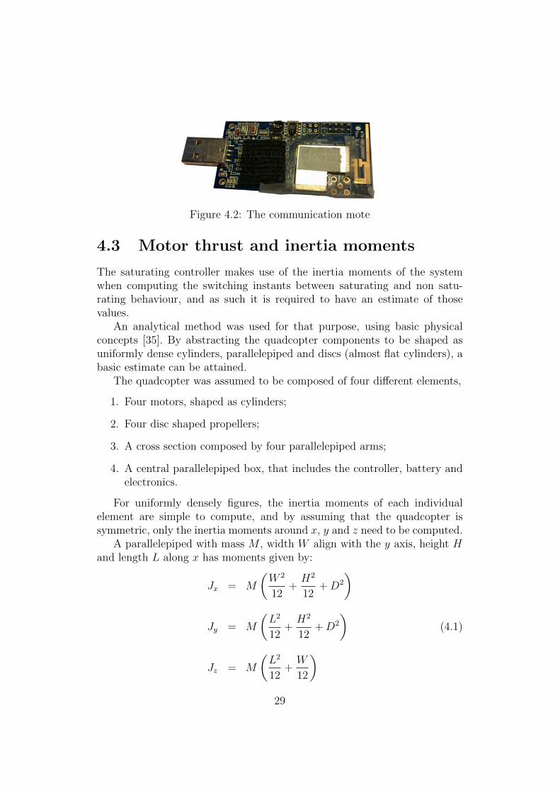
Figure 4.2: The communication mote

4.3 Motor thrust and inertia moments

The saturating controller makes use of the inertia moments of the systemwhen computing the switching instants between saturating and non satu-rating behaviour, and as such it is required to have an estimate of thosevalues.

An analytical method was used for that purpose, using basic physicalconcepts [35]. By abstracting the quadcopter components to be shaped asuniformly dense cylinders, parallelepiped and discs (almost flat cylinders), abasic estimate can be attained.

The quadcopter was assumed to be composed of four different elements,

1. Four motors, shaped as cylinders;

2. Four disc shaped propellers;

3. A cross section composed by four parallelepiped arms;

4. A central parallelepiped box, that includes the controller, battery andelectronics.

For uniformly densely figures, the inertia moments of each individualelement are simple to compute, and by assuming that the quadcopter issymmetric, only the inertia moments around x, y and z need to be computed.

A parallelepiped with mass M , width W align with the y axis, height Hand length L along x has moments given by:

Jx = M

(W 2

12+H2

12+D2

)

Jy = M

(L2

12+H2

12+D2

)

Jz = M

(L2

12+W

12

)(4.1)

29

Figure 4.3: Simplified quadcopter model, with the considered geometric fig-ures in different colours

A cylinder with its height H along z, radius R and mass M has thefollowing moments:

Jx = M

(R2

4+H2

12

)Jy = Jx

Jz = MR2

2

(4.2)

Finally, offsets from the axis of rotation are dealt with by using the par-allel axes theorem [35]. A displacement of D from an axis of rotation adds aterm to the previous formulas:

Jnew = Jcenter +MD2, (4.3)

for each axis of rotation.The motors have the dimensions M = 0.056Kg;R = 0.028m;H = 0.029m

with displacement Dx = 0.31m for two of them and Dy = 0.31mfor the other pair, with Dz = 0.033m, the propellers haveM = 0.008Kg;R = 0.125m;H = 0.01m and the same displacementalong x and y as the motors, with Dz = 0.064m. The centralbox has M = 0.486Kg;L = W0.08m;H = 0.138m and the armsM = 0.015Kg;W = L = 0.013m;H = 0.3m, with no displacement withrespect to their axis of rotation (the arms making a cross centred with thequadcopter frame of reference). The inertia moments are given by summingthe individual parts:

Jx = 2Jmotorx + Jcenterx + 2Jarmx + 2Jpropellerx

Jy = JxJz = 4Jmotorz + Jcenterz + 2Jarmz + 4Jpropellerz

(4.4)

The obtained values were Jx ' 0.02 Kg.m2 and Jz ' 0.032 Kg.m2. Thisis of course a very coarse estimation, that was not changed over the courseof the practical work, since the controller was verified to be robust against

30

Figure 4.4: Thrust measuring stand

errors in the inertia moments [28], and the obtained results compared wellto the simulations.

To get an estimate of the maximum thrust that could be provided by themotors, as well as to get the relationship between PWM and thrust, a simpletest stand was built, that attaches a motor to a wooden arm, sitting on topof a scale. When the motor spins, thrust is generated, and the scale shows adifference in measured weight.

Several experiments were carried out, where the command signal wasmade to vary between the minimum and maximum admissible values. Thisturned out to produce considerably different results for repeated tests, whichcan be traced back to changes in the battery level. Even by starting each testwith a fully-charged battery, going from the maximum admissible value tothe minimum produced significant changes, even with increasing step sizes.In figure 4.5 are depicted the results from three experiments. In the red andblack traces, the command signal started at the maximum value and wasdecreased over the experiment. The blue one depicts an experiment wherethe command signal started at its minimum and was made to increase. It isclear that there is a drop in maximum thrust in this last experiment. The

31

Measurement RegressionBlue cT = 6.665× 10−4 Kg/sRed cT = 7.0657× 10−4 Kg/s

Black cT = 6.9953× 10−4 Kg/s

Table 4.1: Experimental values for the cT constant

100 200 300 400 500 600 700 8000

0.2

0.4

0.6

0.8

PWM [µs]

Thrust

[Kg]

Figure 4.5: Sample of the obtained thrust measurements

battery output current decreased too much and the ESCs were not able toregulate the current that was sent to the motors appropriately.

There is, though, a region that keeps a closer to linear PWM to thrustrelationship, and that was chosen to be the operating range of the outputcommand values from the controller. The speed controllers can receive aPWM command signal with width from 1000µs to 2000µs. From the resultsobtained, and after removing the 1000µs offset, the operating range wasdefined to be in the [100, 600]µs range. The constants cT that were obtainedby linear regression on this region are presented in table 4.1. The used valuewas the lowest one, cT = 6.665×10−4 Kg/s. This is due to the fact that overan experiment, with the battery decreasing, the relationship between PWMand thrust will approach this value. It was deemed more acceptable to riskan underestimation of this constant (that will result in oscillations near thesteady state, due to the controller applying larger torques than the computedones) than an overestimation (that, as the battery decreases, takes controlauthority from the controller, since the saturating limit prevents this effectto be compensated, as it would with, say, a PID controller).

32

Figure 4.6: One degree of freedom test stand

4.4 Test stand

To properly test the controller, it is fundamental to be able to have a sys-tematic way of experimenting with the different parameters, for repeatabilitypurposes. Clearly, it is not possible to test the attitude controller with thequadcopter being in free space, since the lack of position control would makeit easy for the quadcopter to crash, and to explore the controller fully theneed to send aggressive reference values is present.

A test stand was built, that allows only one degree of freedom to beavailable to the quadcopter. It consists of a wooden structure with two woodpillars, see figure 4.6. A metal cable goes through the pillars and passes insideone of the axis of the quadcopter. This allows, by using the two motors onthe orthogonal axis, to change the one of the roll or pitch angles. Due to thesymmetric nature of the frame, it is irrelevant which one.

33

Chapter 5

Results

The one degree of freedom stand makes it impossible to test the controllerwith respect to the yaw. That, together with the absence of propeller dragmeasurements, resulted in the option of testing the controller for its abilityto align the thrust axis, with the drag constant being set as a fifteen timesa lower value, based on measurements done in [27]. The maximum torquesthat were given to the controller were the same as in [28], since that providedgood results and increasing this value would make the problems in the thrustrelationship estimation more evident. The experimental procedure involvessending a−45 degree reference signal, followed by a 45 degree one, resulting ina 90 degree step reference. The parameters used for the experiments are thosein table 5.1. Besides updating the inertia moments to match the real system,the switch curve parameter for ϕ, rϕ, was changed to 0.5. This allows forsmoother transitions between saturated and non-saturated behaviour, whichresulted in a less aggressive behaviour of the system. The parameters relatedto ϑ were omitted, since it is not possible to test for the yaw control on theavailable stand.

Parameter Valueϕl 10π/180 radcϕ 0.817 Nm/radvϕmax 1.425 rad/sδϕ 0.1999 Nms/rad∆ϕ 5π/180 radϕu 175π/180 radrϕ 0.5vϕ 0.1 rad/s

Table 5.1: Experimental parameters

34

Figure 5.1: Frames from a video depicting the quadcopter responding to a90 degree step in the reference. All the results present in this report wereobtained from similar experiments1

5.1 Time-triggered results

The experimental results are depicted in appendix B. There are some im-portant comments to be made, namely, the control torques that are indeedapplied to the system achieve the steady state with an offset, and there issome oscillatory behaviour before stabilizing.

The offset can be explained by the fact that lower torques did not affectthe system as in the rigid body model, since non modelled effects disturbit. The fact that the thrust constant is not exactly known and changes withthe battery level may also lead to sub or overcompensation. This last detailexplain the oscillation in the torques. The system ends up applying a largertorque than the expected one, which leads to more abrupt changes in theangular velocity, that needs to be compensated.

The smaller interpolation constant rϕ makes the transition between satu-rated and non saturated behaviour of the controller more evident, and madefor smoother behaviour. Disturbances, non modelled dynamics and the lowsampling frequency do not allow for a very high value of this variable, as thatwould result in abrupt switching, which adds to the errors in the torques es-timation for creating an oscillating behaviour. Finally, it can be seen thatthere is a variable delay in the system reaction for each experiment. Thiscan also be traced to the battery level influencing the thrust output.

1The full video can be seen at http://youtu.be/cMjN4u3IWhE.

35

5.2 Event-triggered results

The event-triggered results are affected by the low sampling rate that isachievable in the real system. As seen in chapter 3, it is expected for thelinearised and heuristic rules to perform better when the triggering functionis monitoring the state at a higher frequency, and it was not possible toverify that. The presented simulation results match the experiments thatwere done, in the model parameters, initial conditions and reference values.The α and δe parameters used for rules (3.17) and (3.18) are the ones thatin practise provided the best results, or made for important remarks.

For rule (3.12) (figure B.4), the same kind of triggering pattern seenfor the simulation results in figure 3.3 shows up, and a considerable delay isnoticeable, compared to the simulation, as well as some oscillatory behaviour.This can be once again traced back to a non-reliable thrust output from themotors.

The Lyapunov function derivative was computed only at triggering in-stants, meaning that just V (xk) is plotted for the experimental results. Itdoes not allow to see if V (xk) ≤ 0 was violated, but offers some visual inter-pretation of the effect the triggering is having on the rate of change of theLyapunov Function (2.18).

The linearised rule underperformed considerably on the experiments, re-quiring a very conservative value of the constant α to ensure a good be-haviour, as can be seen in figures B.6 and B.8. The main challenge resides instabilizing the angular velocity, task that is made difficult with the combi-nation of errors in the thrust estimation and triggering instants that do notoccur at optimal time. This is due to the fact that both rule (3.12) and (3.17)depend on the artificial torques and damping matrices from the saturatingcontroller to ensure stability, and those translate to control torques that arenot being applied to the system as supposed. The result is a limit cycle kindof behaviour in the angular speed of the system, with the triggering occurringat instants where the controller is unable to compensate for it.

The heuristic rule (3.18) is model independent in the sense that it makesno assumptions about the system, and does not rely on the saturating con-troller to be applied. Hence, while the results still differ from the simulation(the controller faces the same challenges as in the time-triggered case), theperformance either in terms of triggering instants and overall system be-haviour was found to be significantly better, see figure B.10. Note that,since the attitude estimation always carry some noise, the absence of trigger-ing found for the steady state does not translate to the experimental results(figure B.12). The results obtained in terms of triggering instants are sum-marized in table 5.2, for the first 5 seconds of each experiment.

36

Rule Control updates(3.12) 160 (64%)

(3.17), α = 0.1 163 (65%)(3.17), α = 0.01 177 (71%)(3.18), δe = 0.1 69 (28%)(3.18), δe = 0.01 214 (86%)

Baseline 250 (100%)

Table 5.2: Triggering instants results

It is clear that with this experimental conditions, the heuristic rule (3.18)provides the best results. With uncertainties in the applied torques and lowsampling frequency, the simulation results from table 3.2 can not be verified,and since the heuristic rule is independent from the system and controllermodels, it does not suffer from those facts the same way as rules (3.12) and(3.17).

37

Chapter 6

Conclusions

During this project, the saturating controller proposed in [28] was studiedand implemented experimentally for the first time, as far as the author couldassert. An event-triggering rule to work with it was derived, and its sta-bilizing properties were verified experimentally, with a linearised rule beingproposed to minimize inter-sampling computations.

Two major factors limited the obtained results, namely, the inability toprovide more than 50 Hz for the sampling frequency of the controller, dueto the embedded platform used for its implementation, and the fact that areliable application of the computed torques was not possible to attain.

Without a very good estimation of the fundamental values of the quad-copter model, specially, in the case of this specific controller, the PWM tothrust relationship for the motors, there are no practical advantages in usingthe proposed controller over a simple PID application. This is due to the PIDbeing able to correct errors in the attitude by changing the torques withoutbound, while the saturating controller has a specified limit.

Having a better identified system model, and a more powerful embeddedplatform for the computations, it would be possible to perform a more sys-tematic controller characterization and tuning, by specifying some measureof performance to be achieved (settling time of the thrust vector displacementangle, for instance), and select the parameters that minimize it.

6.1 Future work

The attitude control problem for a quadcopter has been extensively studiedbefore, as exposed in chapter 2. It is nevertheless an interesting propositionto study, implement and benchmark several different controllers on the same,well modelled, quadcopter.

38

Such comparison was not found, at least not in a systematic, repeatablemanner, and it could offer some useful insight on whether it is worthy tokeep developing new controllers, besides the obvious academic interest.

The event-triggering attitude control of a quadcopter may be of usefulapplication in a scenario where a multitude of agents are operating towardsa common goal. Distributed and autonomous control of a group of agentshas been subject of recent research [5] [11] [14] [19], just to name a few. Inthis framework, there is no central planning of how the different agents willbehave to reach a certain objective, and they rely on communication betweenthemselves to coordinate. Having an on board attitude control system thatonly needs attention on a small percentage of the sampling instants allowsfor the remaining to be devoted to communication and planning tasks.

Algorithms like the one proposed in [24] allow for impressive group be-haviour of quadcopters, but no autonomous group coordination is present.

One challenge to address would be the construction of a distributed algo-rithm that would enable autonomous group formation of quadcopters, whileachieving some sort of performance criteria.

39

Appendix A

Linearised triggering rulederivation

We need to compute the partial derivatives that composes ∇T(q) in orderto apply (3.17) With:

A =√

1− q2pk

B =√

1− q2wk

C = cϑ

∫ ϑk

0

Λϑuϑl

(ε)dε

D =cϕA

E =cϑB

F = arccos(qwk)

G = arccos(qpk)

we have:

40

∂T

∂qx

∣∣∣∣t=tk

=

DΛϕu

ϕl(ϕk)− q3

pkC

−qzkq3pkEΛϑu

ϑl(ϑk)

0

∂T

∂qy

∣∣∣∣t=tk

=

qzkq

3pkEΛϑu

ϑl(ϑk)

DΛϕuϕl

(ϕk)− q3pkC

0

∂T

∂qz

∣∣∣∣t=tk

=

qykq

3pkEΛϑu

ϑl(ϑk)

−qxkq3pkEΛϑu

ϑl(ϑk)

q4pkEΛϑu

ϑl(ϑk)

.

∂T

∂qp

∣∣∣∣t=tk

and∂T

∂qw

∣∣∣∣t=tk

will depend on the value of ϕ and ϑ, respectively,

due to (2.14). Since∂ϕ

∂qp= − 2√

1− q2p

, we have, for 0 ≤ ϕ ≤ ϕl:

∂T

∂qp

∣∣∣∣t=tk

=

(−2D

A+

2qpkDG

A2− 3q2

pkC

)qxk + 3qzkqykq

2pkEΛϑu

ϑl(ϑk)

(−2D

A+

2qpkDG

A2− 3q2

pkC

)qyk − 3qzkqxkq

2pkEΛϑu

ϑl(ϑk)

4qzkq3pkEΛϑu

ϑl(ϑk)

for ϕl < ϕ ≤ ϕu:

∂T

∂qp

∣∣∣∣t=tk

=

(ϕlDqpkA2

− 3q2pkC

)qxk + 3qzkqykq

2pkEΛϑu

ϑl(ϑk)

(ϕlDqpkA2

− 3q2pkC

)qyk − 3qzkqxkq

2pkEΛϑu

ϑl(ϑk)

4qzkq3pkEΛϑu

ϑl(ϑk)

41

and, for ϕu < ϕ ≤ π:

∂T

∂qp

∣∣∣∣t=tk

=

(− 2DϕlA (ϕu − π)

+Dϕlqpk (2G− π)

A2 (ϕu − π)− 3q2

pkC

)qxk + 3qzkqykq

2pkEΛϑu

ϑl(ϑk)

(− 2DϕlA (ϕu − π)

+Dϕlqpk (2G− π)

A2 (ϕu − π)− 3q2

pkC

)qyk − 3qzkqxkq

2pkEΛϑu

ϑl(ϑk)

4qzkq3pkEΛϑu

ϑl(ϑk)

For ϑ = 2 arccos(qw) we get

∂ϑ

∂qw= − 2√

1− q2w

and∂(ϑ)2

∂qw=

−8 arccos(qw)√1− q2

w

. When 0 ≤ ϑ ≤ ϑl,∫ ϑ(t)

0Λϑuϑl

(ε)dε =ϑ2

2and, as such:

∂T

∂qw

∣∣∣∣t=tk

=

4q3pkqxkEF +

2qwkqzkq

3pkqykEF

B2−

2qzkq3pkqykE

B

4q3pkqykEF −

2qwkqzkq

3pkqxkEF

B2+

2qzkq3pkqxkE

B

2qzkq4pkqwk

EF

B2−

2qzkq4pkE

B

When ϑl < ϑ ≤ ϑu,

∫ ϑ(t)

0Λϑuϑl

(ε)dε =ϑ2l

2+ ϑl (ϑ− ϑl):

∂T

∂qw

∣∣∣∣t=tk

=

2ϑlq3pkqxkE +

ϑlqwkqzkq

3pkqykE

B2

2ϑlq3pkqykE −

ϑlqwkqzkq

3pkqxkE

B2

ϑlqzkq4pkqwk

E

B2

Finally, for ϑu ≤ ϑ ≤ π, the integral becomes

ϑ2l

2+ ϑl (ϑu − ϑl) +

ϑl (ϑ2 − ϑ2

u)

2 (ϑu − π)+ϑlπ (ϑu − ϑ)

ϑu − πand the last partial derivative is

42

∂T

∂qw

∣∣∣∣t=tk

=

−2q3pkqxkϑlE

(π − 2F

ϑu − π

)−

2qzkq3pkqykϑlE

B (ϑu − π)+qzkq

3pkqwk

qykϑl (2F − π)E

B2 (ϑu − π)

−2q3pkqykϑlE

(π − 2F

ϑu − π

)+

2qzkq3pkqxkϑlE

B (ϑu − π)−qzkq

3pkqwk

qxkϑl (2F − π)E

B2 (ϑu − π)

−2qzkq

4pkEϑl

B (ϑu − π)−qzkq

4pkqwk

Eϑl (π − 2F )

B2 (ϑu − π)

43

Appendix B

Experimental results

−0.2

−0.1

0

0.1

0.2

[N.m

]

−1

0

1

2

3

[rad

/s]

0 0.5 1 1.5 2 2.5−0.8

−0.6

−0.4

−0.2

0

Time [s]

[N.m

.rad

/s]

0 0.5 1 1.5 2 2.50

20

40

60

80

100

Time [s]

Deg

rees

Figure B.1: Simulated results for the single axis experience

−0.2

−0.1

0

0.1

0.2

[N.m

]

−1

0

1

2

3

[rad

/s]

0 0.5 1 1.5 2 2.5−0.8

−0.6

−0.4

−0.2

0

[N.m

.rad

/s]

0 0.5 1 1.5 2 2.50

20

40

60

80

100

Deg

rees

Figure B.2: Experimental results for the single axis experience

44

−0.2

−0.1

0

0.1

0.2

[N.m

]

−1

0

1

2

3

[rad

/s]

−0.8

−0.6

−0.4

−0.2

0

[N.m

.rad

/s]

0

20

40

60

80

100

Deg

rees

0 0.5 1 1.5 2 2.5Time [s] 0 0.5 1 1.5 2 2.5Time [s]

Figure B.3: Simulated results for the experimental setup with rule (3.12)

−0.2

−0.1

0

0.1

0.2

[N.m

]

−1

0

1

2

3

[rad

/s]

−0.8

−0.6

−0.4

−0.2

0

[N.m

.rad

/s]

0

20

40

60

80

100

Deg

rees

0 0.5 1 1.5 2 2.5Time [s] 0 0.5 1 1.5 2 2.5Time [s]

Figure B.4: Experimental results for rule (3.12)

45

−0.2

−0.1

0

0.1

0.2

[N.m

]

−2

0

2

4

[rad

/s]

−1

−0.5

0

0.5

[N.m

.rad

/s]

0

20

40

60

80

100

Deg

rees

0 0.5 1 1.5 2 2.5Time [s] 0 0.5 1 1.5 2 2.5Time [s]

Figure B.5: Simulated results for the linearised rule (3.17). α = 0.1

−0.2

−0.1

0

0.1

0.2

[N.m

]

−1

0

1

2

3

[rad

/s]

−1

−0.8

−0.6

−0.4

−0.2

0

[N.m

.rad

/s]

0

20

40

60

80

100

Deg

rees

0 0.5 1 1.5 2 2.5Time [s] 0 0.5 1 1.5 2 2.5Time [s]

Figure B.6: Experimental results for the linearised rule, α = 0.1

46

−0.2

−0.1

0

0.1

0.2

[N.m

]

−1

0

1

2

3

4

[rad

/s]

−1

−0.8

−0.6

−0.4

−0.2

0

[N.m

.rad

/s]

0

20

40

60

80

100

Deg

rees

0 0.5 1 1.5 2 2.5Time [s] 0 0.5 1 1.5 2 2.5Time [s]

Figure B.7: Simulated results for rule (3.17), α = 0.01

−0.2

−0.1

0

0.1

0.2

[N.m

]

−1

0

1

2

3

[rad

/s]

−0.8

−0.6

−0.4

−0.2

0

[N.m

.rad

/s]

0

20

40

60

80

100

Deg

rees

0 0.5 1 1.5 2 2.5Time [s] 0 0.5 1 1.5 2 2.5Time [s]

Figure B.8: Experimental results for rule (3.17), α = 0.01

47

−0.2

−0.1

0

0.1

0.2

[N.m

]

−1

0

1

2

3

[rad

/s]

−0.6

−0.4

−0.2

0

0.2

[N.m

.rad

/s]

0

20

40

60

80

100

Deg

rees

0 0.5 1 1.5 2 2.5Time [s] 0 0.5 1 1.5 2 2.5Time [s]

Figure B.9: Simulated results for the heuristic rule (3.18), δe = 0.1

−0.2

−0.1

0

0.1

0.2

[N.m

]

−1

0

1

2

3

[rad

/s]

−0.8

−0.6

−0.4

−0.2

0

[N.m

.rad

/s]

0

20

40

60

80

100

Deg

rees

0 0.5 1 1.5 2 2.5Time [s] 0 0.5 1 1.5 2 2.5Time [s]

Figure B.10: Experimental results for rule (3.18), δe = 0.1

48

−0.2

−0.1

0

0.1

0.2

[N.m

]

−1

0

1

2

3

[rad

/s]

−0.6

−0.4

−0.2

0

0.2

[N.m

.rad

/s]

0

20

40

60

80

100

Deg

rees

0 0.5 1 1.5 2 2.5Time [s] 0 0.5 1 1.5 2 2.5Time [s]

Figure B.11: Simulated results for rule (3.18), δe = 0.01

−0.2

−0.1

0

0.1

0.2

[N.m

]

−1

0

1

2

3

[rad

/s]

−0.8

−0.6

−0.4

−0.2

0

[N.m

.rad

/s]

0

20

40

60

80

100

Deg

rees

0 0.5 1 1.5 2 2.5Time [s] 0 0.5 1 1.5 2 2.5Time [s]

Figure B.12: Experimental results for rule (3.18), δe = 0.01

49

Bibliography

[1] J.R. Ragazzini and G.F. Franklin. Sampled-data control systems.McGraw-Hill series in control systems engineering. McGraw-Hill, 1958.

[2] K.J. Astrom and B. Wittenmark. Computer controlled systems: the-ory and design. Prentice-Hall information and system sciences series.Prentice-Hall, 1984.

[3] M. D. Shuster. “Survey of attitude representations”. In: Journal of theAstronautical Sciences 41 (Oct. 1993), pp. 439–517.

[4] Panagiotis T. “New control laws for the attitude stabilization of rigidbodies”. In: 13th IFAC Symposium on Automatic Control in Aerospace.1994, pp. 316–321.

[5] T. Vicsek et al. “Novel type of phase transition in a system of self-driven particles”. In: Physical review letters 75.6 (1995), p. 1226.

[6] K. J. Astrom and B. Bernhardsson. “Comparison of periodic and eventbased sampling for firstorder stochastic systems”. In: Proceedings of the14th IFAC World Congress. 1999.

[7] R. Ortega et al. “Putting energy back in control”. In: IEEE ControlSystems Magazine (Apr. 2001), pp. 18–33.

[8] T. Hamel et al. Dynamic Modelling And Configuration StabilizationFor An X4-Flyer. 2002.

[9] H.K. Khalil. Nonlinear Systems. Prentice Hall PTR, 2002. isbn:9780130673893.

[10] P. Pounds et al. “Design of a Four-Rotor Aerial Robot”. In: Aus-tralasian Conference on Robotics and Automation. 2002, pp. 145–150.

[11] A. Jadbabaie, J. Lin, and A. S. Morse. “Coordination of groups of mo-bile autonomous agents using nearest neighbor rules”. In: IEEE Trans-actions on Automatic Control 48.6 (2003), pp. 988–1001.

50

[12] S. Bouabdallah, P. Murrieri, and R. Siegwart. “2004-b, “Design andControl of an Indoor Micro Quadrotor”. In: Proc. of Int. Conf. onRobotics and Automation. 2004.

[13] S. Bouabdallah, A. Noth, and R. Siegwart. “PID vs LQ control tech-niques applied to an indoor micro quadrotor”. In: IEEE Internationalconference on intelligent robots and systems. 2004, pp. 2451–2456.

[14] W. Ren and R. W. Beard. “Consensus Seeking in Multiagent SystemsUnder Dynamically Changing Interaction Topologies”. In: IEEE Trans-actions on Automatic Control 50.5 (2005), p. 655.

[15] A. Tayebi and S. McGilvray. “Attitude stabilization of a VTOL quadro-tor aircraft”. In: Control Systems Technology, IEEE Transactions on 3(Apr. 2006), pp. 562–571.

[16] P. Adigbli et al. “Nonlinear Attitude and Position Control of a Mi-cro Quadrotor using Sliding Mode and Backstepping Techniques”. In:European Micro Air VehicleConference and Flight Competition (2007).

[17] P. Tabuada. “Event-Triggered Real-Time Scheduling of StabilizingControl Tasks”. In: IEEE Transactions on Automatic Control (2007).

[18] Karl J. Astrom. “Event Based Control”. In: Analysis and Design ofNonlinear Control Systems. Ed. by A. Astolfi and L. Marconi. SpringerBerlin Heidelberg, 2008, pp. 127–147.

[19] D. Dimarogonas and E. Frazzoli. “Distributed event-triggered controlstrategies for multi-agent systems”. In: Communication, Control, andComputing, 2009. Allerton 2009. 47th Annual Allerton Conference on.IEEE. 2009, pp. 906–910.

[20] W. Premerlani and P. Bizard. Direction Cosine Matrix IMU: Theory.2009.

[21] A. Eqtami, D. Dimarogonas, and K. Kyriakopoulos. “Event-triggeredcontrol for discrete-time systems”. In: American Control Conference(ACC), 2010. IEEE. 2010, pp. 4719–4724.

[22] N.A. Chaturvedi, A.K. Sanyal, and N.H. McClamroch. “Rigid-BodyAttitude Control”. In: Control Systems, IEEE 31.3 (June 2011),pp. 30–51.

[23] N. Marchand, S. Durand, and F. Guerrero-Castellanos. A general for-mula for the stabilization of event-based controlled systems. 2011.

[24] A. Kushleyev, V. Kumar, and D. Mellinger. “Towards A Swarm of AgileMicro Quadrotors”. In: Proceedings of Robotics: Science and Systems.Sydney, Australia, July 2012.

51

[25] D. Lehmann and K. H. Johansson. Event-triggered PI control subjectto actuator saturation. 2012.

[26] Robert E. Mahony, V. Kumar, and P. Corke. “Multirotor Aerial Ve-hicles: Modeling, Estimation, and Control of Quadrotor.” In: IEEERobot. Automat. Mag. (2012), pp. 20–32.

[27] F. Castellanos et al. “Event-triggered nonlinear control for attitudestabilization of a quadrotor”. In: Journal of Intelligent and RoboticSystems (2013).

[28] O. Fritsch, B. Henze, and B. Lohmann. “Fast and Saturating AttitudeControl for a Quadrotor Helicopter”. In: Control Conference (ECC),2013 European (Sept. 2013), pp. 3851 –3857.

[29] Oliver Fritsch, Bernd Henze, Boris Lohmann, et al. “Fast and Saturat-ing Thrust Direction Control for a Quadrotor Helicopter.” In: Automa-tisierungstechnik, vol. 61, no. 3 (Mar. 2013), 172–182.

[30] WPMH Heemels, MCF Donkers, and Andrew R Teel. “Periodic event-triggered control for linear systems”. In: Automatic Control, IEEETransactions on 58.4 (2013), pp. 847–861.

[31] A. Honglei et al. “Backstepping-Based Inverse Optimal Attitude Con-trol of Quadrotor”. In: International Journal of Advanced Robotic Sys-tems (2013).

[32] C. R. Paiva. Os Quaternioes de Hamilton. 2013.

[33] APM:Copter website. url: http://copter.ardupilot.com/.

[34] K. E. Arzen. A simple event-based PID controller.

[35] T. Bresciani. Modelling, Identification and Control of a Quadrotor He-licopter.

[36] G.P. Cyril. The Breguet-Richet Quad-Rotor Helicopter of 1907.

[37] Oemichen 1922. url: http://www.aviastar.org/helicopters_eng/oemichen.php.

52