event related potentials and endogenous temporal pulse
TRANSCRIPT

Event Related Potentials and
Endogenous Temporal Pulse
An Honors Thesis Submitted to the Department of Biology
Harvard College
by
Peter H. Li
In Partial Fulfillment of the Requirements for the Degree of
Bachelor of Arts
in
Neurobiology
Thesis Director: Lecturer in Psychology W. Tecumseh Fitch
Thesis Co-Sponsor: Professor John E. Dowling
Cambridge, MassachusettsApril, 2002

For Mom and Dad
With Love
i

Acknowledgements
I would like to express my appreciation to all friends and family for their kindsupport throughout this project. Special thanks to Mom, Dad, Kuba, John, Andrea,Tiffany, and the Dunster House Opera Cast, Staff, Orchestra, and Board.
This work would not have been possible without the generosity of Dr. Allen Braunand the NIDCD in allowing me to make use of their electroencephalography equip-ment. Furthermore I would particularly like to thank Joe McArdle and Dr. VladimirNechaev, two employees at the NIDCD, for taking me under their wing and sharingtheir experience with me. I am also indebted to Dr. Bernat Kocsis and Dr. JoseCantero at the Harvard Medical School for making themselves available to answer mytechnical questions and inviting me to observe some of their electrophysiological work.
Many, many thanks to my committee for taking the time to read and review mywork, especially Professor Dowling, who has been kind enough to sponsor me beforethe biology department.
Finally, none of this would have been possible without the inspiration of my ad-visor, Dr. W. Tecumseh Fitch. Thank you for sticking with me through a numberof frustrating setbacks, thank you for helping me grow from a Matlab novice intoa master of matrix manipulation, and thank you for devoting your time to get mestarted on this work, meeting me in Washington D.C. and introducing me to the NIH.This has been an incredible learning experience for me, academically, personally, andprofessionally.
ii

Contents
1 Introduction 11.1 EEG and Biology . . . . . . . . . . . . . . . . . . . . . . . . . . . . . 1
1.1.1 Theoretical Basis of EEG . . . . . . . . . . . . . . . . . . . . 21.1.2 Empirical Confirmation of Theoretical Potentials . . . . . . . 81.1.3 Determination of EEG Generators . . . . . . . . . . . . . . . . 15
1.2 EEG and Cognitive Psychology . . . . . . . . . . . . . . . . . . . . . 201.2.1 Event Related Potentials . . . . . . . . . . . . . . . . . . . . . 201.2.2 Standard ERP Waveforms in Psychophysiology . . . . . . . . 211.2.3 Endogenous and Exogenous Components . . . . . . . . . . . . 24
1.3 The Current Study . . . . . . . . . . . . . . . . . . . . . . . . . . . . 241.3.1 Metrical Pattern Processing . . . . . . . . . . . . . . . . . . . 241.3.2 Endogenous Timing . . . . . . . . . . . . . . . . . . . . . . . . 26
2 Materials and Methods 282.1 Subjects . . . . . . . . . . . . . . . . . . . . . . . . . . . . . . . . . . 282.2 Equipment . . . . . . . . . . . . . . . . . . . . . . . . . . . . . . . . . 292.3 Procedures . . . . . . . . . . . . . . . . . . . . . . . . . . . . . . . . . 31
2.3.1 Electrode Layout . . . . . . . . . . . . . . . . . . . . . . . . . 312.3.2 Event Recording . . . . . . . . . . . . . . . . . . . . . . . . . 322.3.3 Electrode Reference . . . . . . . . . . . . . . . . . . . . . . . . 342.3.4 Detection of Overimpeded Electrodes . . . . . . . . . . . . . . 34
2.4 Experimental Paradigm . . . . . . . . . . . . . . . . . . . . . . . . . 352.5 Saccades, Blinks, and Artifact Removal . . . . . . . . . . . . . . . . . 36
3 Results 413.1 Sampling Rate . . . . . . . . . . . . . . . . . . . . . . . . . . . . . . 423.2 Analysis of Button Box Lag Time . . . . . . . . . . . . . . . . . . . . 433.3 Analysis of Subject Performance . . . . . . . . . . . . . . . . . . . . . 463.4 Comparison of ERP Waveforms . . . . . . . . . . . . . . . . . . . . . 51
3.4.1 Isolated Signature of Endogenous Pulse . . . . . . . . . . . . . 513.4.2 Bereitschafts Potential Results . . . . . . . . . . . . . . . . . . 53
3.5 Topographic Plots of Bereitschafts Amplitudes . . . . . . . . . . . . . 56
iii

3.5.1 Evidence for Contingent Negative Variation . . . . . . . . . . 59
4 Discussion 614.1 Signatures of Endogenous Pulse . . . . . . . . . . . . . . . . . . . . . 614.2 Anti-Lateralization Effects . . . . . . . . . . . . . . . . . . . . . . . . 624.3 Continuing Research . . . . . . . . . . . . . . . . . . . . . . . . . . . 62
4.3.1 Clarifying Anti-Lateral Effects . . . . . . . . . . . . . . . . . . 634.3.2 Event-Related Spectral Dynamics . . . . . . . . . . . . . . . . 63
4.4 Conclusions . . . . . . . . . . . . . . . . . . . . . . . . . . . . . . . . 64
A Matlab Code A-1A.1 CStruct Toolbox . . . . . . . . . . . . . . . . . . . . . . . . . . . . . A-1
A.1.1 fread cs.m . . . . . . . . . . . . . . . . . . . . . . . . . . . . . A-1A.1.2 sizeof cs.m . . . . . . . . . . . . . . . . . . . . . . . . . . . . . A-4
A.2 Neuroscan Toolbox . . . . . . . . . . . . . . . . . . . . . . . . . . . . A-5A.2.1 calibERP.m . . . . . . . . . . . . . . . . . . . . . . . . . . . . A-5A.2.2 collectCNT.m . . . . . . . . . . . . . . . . . . . . . . . . . . . A-7A.2.3 epochData.m . . . . . . . . . . . . . . . . . . . . . . . . . . . A-11A.2.4 fixHeader.m . . . . . . . . . . . . . . . . . . . . . . . . . . . . A-14A.2.5 loadEEG.m . . . . . . . . . . . . . . . . . . . . . . . . . . . . A-16A.2.6 plotWaves.m . . . . . . . . . . . . . . . . . . . . . . . . . . . . A-20A.2.7 topoPlot.m and topoInterp.m . . . . . . . . . . . . . . . . . . A-22
A.3 Header Files . . . . . . . . . . . . . . . . . . . . . . . . . . . . . . . . A-24A.3.1 GEN HEAD.m . . . . . . . . . . . . . . . . . . . . . . . . . . A-24
iv

List of Figures
1.1 Dipole Model of Neural Activity . . . . . . . . . . . . . . . . . . . . . 41.2 ‘Closed’ vs. ‘Open’ Fields Produced by Brain Structures . . . . . . . 61.3 Geometry of Equations 1.2, 1.3, and 1.4 . . . . . . . . . . . . . . . . 71.4 Medial and Lateral segments of the Superior Olive . . . . . . . . . . . 91.5 Polar organization of the Medial Superior Olive . . . . . . . . . . . . 101.6 Topographical Plot of Electric Fields from the Superior Olive . . . . . 121.7 Superior Olive Recordings versus Ideal Dipole Layer . . . . . . . . . . 141.8 Schematized Representation of Typical Bereitschafts Potential . . . . 23
2.1 Neuromedical Supplies Quick-Cap . . . . . . . . . . . . . . . . . . . . 302.2 Neuroscan SynAmps and STIM Equipment . . . . . . . . . . . . . . . 312.3 Electrode Locations . . . . . . . . . . . . . . . . . . . . . . . . . . . . 332.4 Extensor Digitorum . . . . . . . . . . . . . . . . . . . . . . . . . . . . 332.5 Electrode Calibration Sample from Data Set 2 . . . . . . . . . . . . . 352.6 Contamination of EEG electrodes by EOG activity . . . . . . . . . . 38
3.1 Power Spectrum from Standard EEG Data Set . . . . . . . . . . . . . 433.2 Representative Button Box versus EMG . . . . . . . . . . . . . . . . 443.3 Distribution of Button Lag Times . . . . . . . . . . . . . . . . . . . . 453.4 Plot of Intervals Between Sequential Events . . . . . . . . . . . . . . 493.5 Ratios of Sequential Intervals in the Complex Rhythm Trials . . . . . 503.6 Histogram of Intervals in the Complex Rhythm Trials . . . . . . . . . 503.7 Possible Signature of Internal Pulse . . . . . . . . . . . . . . . . . . . 523.8 Canonical Bereitschafts Result . . . . . . . . . . . . . . . . . . . . . . 533.9 ERP Results from Experimental Conditions . . . . . . . . . . . . . . 543.10 Topographic Maps of BP Amplitudes . . . . . . . . . . . . . . . . . . 583.11 Evidence for CNV in Syncopated Trials . . . . . . . . . . . . . . . . . 60
v

Abstract
In this study, we attempt to use Electroencephalography, the measurement ofelectrical potentials from the surface of the scalp, to reveal the underlying mechanismbehind the performance of endogenously-timed, metrical behaviors in humans. Itis proposed that the timing of metrically patterned voluntary movements relies onthe brain’s ability to generate and maintain an internal temporal pulse. We describeseveral hypothetical signatures of this internal pulse and then seek them out in a seriesof experiments based on the Event-Related Potentials paradigm. Results providequalified support for the primary hypothesis; we record a possible waveform signatureof the endogenous pulse as well as demonstrate the likely ability of mental pulses toact as internal cues for normally externally triggered Contingent Negative Variation.Finally, we discover an unexpected anti-lateralization in the normally contralaterallybiased Motor Readiness Potential.
vi

Chapter 1
Introduction
This introduction is divided into three sections. The second and third sections relate
directly to the current study, while the first provides a general overview of biological
issues in electroencephalography. This overview is provided to explore a few quick
and simple mathematical models of the relationship between underlying bioelectrical
activity and the extracranial potentials measured by psychophysiologists. It also
presents some of the new ways in which psychophysiological results can be related to
underlying biological mechanisms.
1.1 Electroencephalography and Biology
The Event Related Potential is a special paradigm of a more general physiological
measure, the Electroencephalogram (EEG). EEG is the recording of electric poten-
tials at the scalp of a living subject (usually human). Presumably these extracranial
potentials are produced by electrical currents associated with underlying neural activ-
1

CHAPTER 1. INTRODUCTION 2
ity.1 More formally, EEG records potential difference, with a typical amplitude range
of -100 to 100 µV, and meaningful frequencies between 0.1 and 55Hz [7]. Higher fre-
quencies are usually present in the signal, but typically reflect fast muscle fluctuations
of little neurobiological significance or spurious external noise (e.g. 60Hz AC current,
70-100Hz computer monitors refresh rates, etc.) [6].
There are two major paradigms historically used in considering EEG voltages:
bipolar recording and referenced recording. In bipolar recording, specific pairs of
electrodes are used to monitor voltages between individual scalp locations. In refer-
enced recording, a full array of scalp electrodes is referenced off of a single assumed
baseline electrode such as the nose or the ears, where no neural activity is expected.
Theoretically, in a referenced recording scheme any two electrodes can be picked out
of the array and differenced, yielding the equivalent bipolar values for that pair. This
process cannot be reversed however, thus bipolar recordings inherently carry less
information than their referenced counterparts.2
1.1.1 Theoretical Basis of EEG
The precise relationship between measured scalp potentials and underlying electrical
activity within the brain has long been controversial and is not currently entirely
understood. However, EEG does seem to be based on the same fundamental bioelec-
trical events that are monitored in other electrophysiological recording paradigms.
1This proposition is investigated more thoroughly in Sections 1.1.1 and 1.1.2 below.2Even if the individual differences between every electrode in an array are known, an unambigu-
ous single reference reconstruction is not possible because the brain is not a homogeneous medium.Perhaps it would be more formally accurate to say that ‘bipolar recordings are less internally consis-tent than their referenced counterparts.’ However, for our purposes the important conclusion is thata bipolar representation can be fully generated from a single reference data set, while the oppositeis not practically possible.

CHAPTER 1. INTRODUCTION 3
Information transmission within the nervous system operates through electrochemical
gradients propagating along and between neuronal cell processes. This propagation
of current within and between neurons naturally produces complimentary current
flows in the surrounding extracellular medium. Thus monitoring extracellular poten-
tials via microelectrode can be quite an effective way of gauging the internal activity
of nearby cells, a characteristic that is exploited in the extracellular unit recording
paradigm.
Furthermore, under appropriate conditions, the flow of current across cell mem-
branes and along neural processes results in a net electric dipole detectable outside the
cell. For example, in the simplified model neuron depicted in Figure 1.1, excitatory
synaptic contacts at the soma cause current to flow into the cell body and towards the
dendritic processes, where the current eventually crosses back through the membrane
and returns to the vicinity of the cell body through the extracellular medium. The
source-sink behavior of the neuron, combined with its particular directional geometry,
produces a dipolar charge separation [19] [27].
An important distinction between EEG and unit recording is that EEG monitors
macroelectrical fields, in contrast to the short-range potential fluctuations observable
with microelectrodes. For a signal to be detectable at the scalp surface, the number,
relative orientation, and synchronicity of the underlying neurons is extremely impor-
tant. For example, a structure like the thalamus cannot produce measurable scalp
potentials, because the fields generated by the randomly distributed individual neural
dipoles tend to cancel each other out. On the other hand, regions in which neurons or
neural processes are more systematically organized exhibit superpositional summation
and can therefore generate potentials measurable at the scalp [6]. Importantly, the

CHAPTER 1. INTRODUCTION 4
Figure 1.1: Dipole Model of Neural ActivityA dipole model of an excitatory synapse. In the top schematic, the excitatory contact causes anet current flow into the soma and out of the dendrites. Thus the dendrites are current sources,while the cell body acts as a current sink. This arrangement results in numerous positive andnegative potential wells, generating a net dipole. An inhibitory synapse produces an equivalentreversed current loop and opposite dipole. Current flow within the neuron tends to involve the somaand dendrites rather than the axon because the axon is the path of greatest resistance. Based on [19].

CHAPTER 1. INTRODUCTION 5
cortex is one such region, organized with enough directionality that cortical activity
can be reflected in EEG readings.
Although we must always bear in mind that EEG potentials can only be produced
by brain structures with the proper geometry, we should also recognize that this can be
an advantage as well as a limitation. If we received scalp signals from every part of the
brain simultaneously, the resultant waveform would be far too complicated to admit
the type of analysis and interpretation that is currently possible [6]. Furthermore,
since only certain neural clusters are valid candidates for the production of scalp
potentials, we are given a slight head start in determining the possible intracranial
sources of an observed EEG effect.
A rough model of the importance of cooperative neuron orientation in producing
a measurable EEG signal is depicted in Figure 1.2. A more quantitative comparison
of various possible arrangements is considered in Figure 1.3. Potential at a distance
d from a point charge of magnitude q is defined as the scalar quantity:
V =kq
d(1.1)
where k is Coulomb’s Constant (= 8.99× 10⁹), based on ε0, the Permittivity of Free
Space. Distance and charge are measured in International Standard units of meters
and Coulombs, potential difference is in Volts.
In the case of a single dipole with equal but opposite charges of magnitude q and
axial distances y1 and y2 (see Figure 1.3) this yields a total potential at a distance d
in the axial direction of:
Vdipole = k
(q
y1
− q
y2
)= kq
(y2 − y1)
y1y2
(1.2)
The case of a dipole layer is somewhat more complicated. If we model the dipole

CHAPTER 1. INTRODUCTION 6
Figure 1.2: ‘Closed’ vs. ‘Open’ Fields Produced by Brain StructuresIn the structure at top, the individual neurons are oriented haphazardly, resulting in a “net closedfield.” At bottom, conversely, the neurons are arranged in parallel such that their potentials sumto create a “net open field.”

CHAPTER 1. INTRODUCTION 7
Figure 1.3: Geometry of Equations 1.2, 1.3, and 1.4Single dipole at left, dipole layer represented as two parallel charged discs at right.
layer as two parallel, uniformly charged discs (see Figure 1.3), then for each disc of
total radius R and total charge Q, the total potential at distance z can be calculated
as the integral over r:
Vdisc =
∫ R
0
2kQ
R2√
r2 + z2dr =
2kQ
R2
(√R2 + z2 − z
)(1.3)
If we apply Equation 1.3 to each of the charged discs in our dipole model and
sum the resulting potentials, we arrive at the potential equation for the whole dipole
layer:
Vlayer =2kQ
R2
[(z2 +
√R2 + z2
1
)−
(z1 +
√R2 + z2
2
)](1.4)
Equations 1.2 and 1.4 quantitatively demonstrate the importance of cooperatively
oriented neuron layers in the generation of measurable EEG signals. As long as we
remain close to the dipole layer, we can assume that R� z. This simplifies Equation
1.4:
R� z =⇒ Vlayer ≈2kQ(z2 − z1)
R2(1.5)

CHAPTER 1. INTRODUCTION 8
Thus as long as we remain close to the dipole layer relative to the total size of the
layer, the potential remains constant. This is a considerable improvement in signal
persistence over the inverse square degradation from a single dipole. Of course, these
equations concern potentials produced by idealized cells and cell layers; in practice, we
would expect most brain potential fields to decay at some intermediate rate between
these ideals.
1.1.2 Empirical Confirmation of Theoretical Potentials
Section 1.1.1 above presents a model for the plausible biological basis of EEG. In this
section, we will briefly consider a set of empirical results that appear to support that
theoretical model.3
The Superior Olivary Nucleus in the pons Varolii, an early stop in the primary au-
ditory pathway, provides a particularly good system for investigating the dependence
of potential fields on relative neuron orientations. As Figure 1.4 shows, the supe-
rior olive is composed of separate medial and lateral structures: the lateral segment
has a characteristic ‘S’ shape while the medial segment takes on a relatively simple
plate form. Significantly, these structures are quite distinct on a synaptic level. The
connectivity of the lateral olivary body has no particular polarity [28]. Therefore,
according to the model presented in 1.1.1, the lateral body should not produce a
measurable external field.
The medial segment, on the other hand, has a considerable directional bias to its
organization, depicted in Figure 1.5. The schematic also illustrates the duality of this
organization; one set of tightly-packed, parallel fibers projects from the contralateral
3The following analysis is inspired by Nunez [19], but our conclusions are slightly different fromthose presented in Chapter 3 of his book.

CHAPTER 1. INTRODUCTION 9
Figure 1.4: Medial and Lateral segments of the Superior OliveCoronal section through the superior olive of a cat. The medial and lateral structures are clearlydistinct, the lateral exhibiting its characteristic ‘S’ shape. Note the extensive contra- and ipsilateralafferent fiber innervation (ipsilateral is to the right, contralateral to the left in this figure). Thearrow marks a possible path of electrode insertion for recording experiments. From [4]

CHAPTER 1. INTRODUCTION 10
Figure 1.5: Polar organization of the Medial Superior OliveThe stained image (×620) exhibits the tightly-packed, parallel fibers responsible for the strongpolarity of the medial olive; the nerve bundles are almost striate in appearance. The schematicgives a more clear view of the polarity of the innervations; one set of contralateral projections, oneset of ipsilateral. From [28]
ear and contacts olivary neurons on one side, while projections from the ipsilateral side
make contacts on the same cells from the opposite direction. Every cell in the medial
superior olive receives innervation from both ears (and therefore both directions), a
property which makes sense given the well established role of the superior olive in
sound localization [4].
The coordinated orientation of the fibers depicted in Figure 1.5 makes the medial
structure a prime candidate for detecting dipole potentials. However, the symmetric

CHAPTER 1. INTRODUCTION 11
innervation from opposite sides could be a source of concern; the innervations from
opposite ears appear to work against each other, producing interfering potential fields
that threaten to cancel each other out. The saving grace of the system is that each
major innervation is associated with a separate ear. Therefore, to protect the signal
from attenuation, it is simply a matter of stimulating one ear significantly more than
the other.
In an experiment by Biedenbach and Freeman [4] [19], recordings were taken from
the superior medial olive of cats during monaural stimulation. The electrode was
slowly moved through the olivary nucleus from the medial segment to the lateral
segment along the path described by the arrow in Figure 1.4. Table 1.1 summarizes
the results under ipsilateral stimulation. The original distances given indicate the
electrode’s depth along the path through the structure, but we are more interested in
the distance from the center of the theorized dipole, or in other words the isopotential
point, which we estimated to be at ≈ 4.65mm.4 For each distance, a large number
of observations (N = 20-100) were averaged to get mean potential readings. A topo-
graphical plot of the observed fields under ipsilateral stimulation is also provided in
Figure 1.6.
Figure 1.7 shows a plot of the experimental data, with an overlaid theoretical
curve for an ideal dipole layer from our Equation 1.4. There are several important
points to draw from Biedenbach and Freeman’s results.
First, the geometry of the fields agrees with our theoretical dipole model. The
zero potential turnaround point lies very near the midline of the medial segment
4This choice may seem unusual since the point at 4.6mm technically has crossed the isopotentialline already. 4.55mm is actually the point intermediate between the last negative reading and thefirst positive one. However, in viewing the data holistically, 4.65mm appears to be a better estimateof the center line than 4.55mm.

CHAPTER 1. INTRODUCTION 12
Distance along Directed Distance from Potential Number ofPath (mm) Estimated Dipole Center (mm) (µV) Observations
3.5 -1.15 26 1004.4 -0.25 137 204.5 -0.15 87 204.6 -0.05 -66 204.7 +0.05 -100 204.8 +0.15 -113 204.9 +0.25 -154 205.0 +0.35 -180 205.5 +0.85 -87 206.0 +1.35 -40 207.0 +2.35 -18 50
Table 1.1: Potentials Measured at the Superior Olive in Cats [4]
Figure 1.6: Topographical Plot of Electric Fields from the Superior OliveElectric fields of the superior olive under ipsilateral stimulation. The black line represents theturnaround point, i.e. the center of the dipole layer. The contours illustrate the field localizationaround the medial segment; the lateral segment seems to make no significant contribution. From [4]
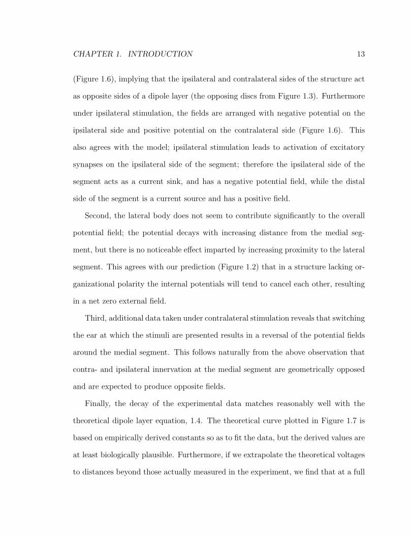
CHAPTER 1. INTRODUCTION 13
(Figure 1.6), implying that the ipsilateral and contralateral sides of the structure act
as opposite sides of a dipole layer (the opposing discs from Figure 1.3). Furthermore
under ipsilateral stimulation, the fields are arranged with negative potential on the
ipsilateral side and positive potential on the contralateral side (Figure 1.6). This
also agrees with the model; ipsilateral stimulation leads to activation of excitatory
synapses on the ipsilateral side of the segment; therefore the ipsilateral side of the
segment acts as a current sink, and has a negative potential field, while the distal
side of the segment is a current source and has a positive field.
Second, the lateral body does not seem to contribute significantly to the overall
potential field; the potential decays with increasing distance from the medial seg-
ment, but there is no noticeable effect imparted by increasing proximity to the lateral
segment. This agrees with our prediction (Figure 1.2) that in a structure lacking or-
ganizational polarity the internal potentials will tend to cancel each other, resulting
in a net zero external field.
Third, additional data taken under contralateral stimulation reveals that switching
the ear at which the stimuli are presented results in a reversal of the potential fields
around the medial segment. This follows naturally from the above observation that
contra- and ipsilateral innervation at the medial segment are geometrically opposed
and are expected to produce opposite fields.
Finally, the decay of the experimental data matches reasonably well with the
theoretical dipole layer equation, 1.4. The theoretical curve plotted in Figure 1.7 is
based on empirically derived constants so as to fit the data, but the derived values are
at least biologically plausible. Furthermore, if we extrapolate the theoretical voltages
to distances beyond those actually measured in the experiment, we find that at a full

CHAPTER 1. INTRODUCTION 14
Figure 1.7: Superior Olive Recordings versus Ideal Dipole LayerThe experimental data from Table 1.1 [4] are plotted as discrete points. Overlaid is the curvegiven by the theoretical dipole layer equation, 1.4. The values used for R, kQ, and (z2 − z1) wereestimated empirically to approximate the experimental data.

CHAPTER 1. INTRODUCTION 15
centimeter away from the dipole center the signal strength is still ≈ 0.8µV .5 Thus,
even for the relatively small dipole layer we have modeled here (R = 750µm), a
measurable potential extends roughly 1cm beyond the center of the structure. This is
strong indirect support for the assertion that EEG scalp recording can legitimately be
tied to activity in the cortex, a structure that lies just millimeters below the surface
of the scalp and exhibits organizational polarity similar to that in the superior olive,
but whose dipole layers could easily cover several times the area postulated here [19].
1.1.3 Determination of EEG Generators
Sections 1.1.1 and 1.1.2 present a rough model for the way in which scalp potentials
can be generated by activity in intracranial neural generators. However, a general
understanding of how underlying biological processes lead to EEG signals does not
necessarily clarify the biological significance of newly observed EEG effects. In other
words, if we had a full description of underlying activity in the brain, then perhaps
we could, to a good approximation, calculate the appropriate scalp potentials based
on theoretical equations; but the reverse is not necessarily true. Thus although we
can be confident that scalp potentials reflect brain activity, usually very consistently,
the precise relationship between an EEG waveform and an underlying cognitive or
physiological state is seldom transparent. This issue can be addressed in a number of
ways, and new technologies now offer additional possible approaches [6].
5In a typical setup, noise begins to obscure the EEG at a signal strength of ≈ 1µV

CHAPTER 1. INTRODUCTION 16
Animal Models
Many researchers have tried to investigate the underlying biology of EEG waveforms
using comparative approaches in animals. Furthermore, a number of animal exper-
iments have useful implications for EEG research even if this was not the primary
aim of the work. The results of Biedenbach and Freeman, presented above in Section
1.1.2, are a good example of an animal electrode study yielding data that is very
useful to the EEG community.
The obvious advantage of animal systems is that they allow considerably more
freedom in the use of invasive methods. This includes the use of intracranial depth
electrodes to get a much closer, less obstructed view of the potentials produced by
specific brain regions, as well cruder ablative lesioning or pharmacological approaches
that would not be ethical in humans [24]. Particularly helpful is the ability to use
a depth electrode both to measure intracranial signals, and to mark brain regions
histochemically where interesting effects are observed.
A recent trend is to use standard EEG methods, similar to those used in human
studies, to try to observe equivalent waveform effects in animals. If researchers can
infer a connection between known human EEG effects, and an observed animal effect,
then the animal system can be manipulated invasively in an attempt to clarify our
understanding of the animal, and hopefully the human system as well.
Combined Imaging
Another recent trend is combined imaging, in which newer technology is used in
conjunction with EEG to get multiple perspectives on the same effects [6] [1].
Magnetoencephalograpy (MEG), is based on the same underlying biology as EEG,

CHAPTER 1. INTRODUCTION 17
but monitors modulating extracranial magnetic fields rather than electrical potentials
[5]. The advantage of combining MEG with EEG is that the two methods are sensitive
to different types of signals. For example, because of the geometric properties of
magnetic fields, MEG tends to be insensitive to radial currents, i.e. currents moving
from central brain regions towards the scalp. Transverse currents on the other hand,
those which run under the surface of the scalp and parallel to it, generate measurable
extracranial magnetic fields.6 EEG is sensitive to both radial and transverse currents.
Positron Emission Tomography (PET) and Functional Magnetic Resonance Imag-
ing (fMRI) are two technologies which monitor metabolic processes in various parts
of the brain as a way of inferring relative activity [17].7 Because these methods
rely on metabolic effects, they lack the extremely high time resolution of direct elec-
trical or magnetic signals. However, both PET and fMRI are inherently spatially
localized to within about 1cm3 under typical conditions, whereas EEG generators
are generally difficult to localize even to within areas of many centimeters in diam-
eter. Furthermore, PET and fMRI do not have the same sensitivity bias of EEG to
signals originating near the scalp, nor must brain structures conform to a particu-
lar organizational geometry in order to produce PET or fMRI signals [25].8 Thus,
again, combined imaging offers the advantage of sensitivity to qualitatively different
measures of activity.
6The cortex is organized such that the vast majority of cortical currents run radially, perpendic-ular to the scalp. However, in the sulci, which are the deep furrows and grooves characteristic ofthe human cortex, the synaptic organization is essentially the same but the folding in of the braintissue results in currents that run parallel to the scalp. It is presumed that much of the MEG signaloriginates from these cortical sulci.
7The fundamental idea is that areas receiving more blood flow, consuming more metabolic pre-cursors, or producing more metabolic byproducts must therefore be more biologically active.
8There are, however, other spatial limitations that must be taken into consideration in PET andfMRI. For example, some brain regions cannot be imaged effectively with fMRI due to magneticsusceptibility artifact [25]

CHAPTER 1. INTRODUCTION 18
Combined imaging can be done sequentially or simultaneously. In the former, each
imaging technique is used separately under hopefully accurately replicated experimen-
tal conditions. Slightly more robust, simultaneous imaging uses both techniques in
the same experimental trial.9
Clinical Cases
Finally, there are a number of avenues of EEG research based on human clinical
cases. One of the most interesting of these is human intracranial electrode studies
in epilepsy patients. If a patient suffers from severe, chronic seizures that do not
respond to antiepileptic drugs, he or she may consider undergoing neurosurgery to
excise the epileptic focus, the discrete brain region that is sometimes responsible for
initiating more general epileptic activity. Of course, before surgery can be planned,
it is extremely important to make certain that the epileptic source region is identified
securely. Furthermore, it is important that the region identified as the epileptic focus
and selected for resection is not also critical to specific cortical functions such as
language or motor control.
Thus, in some cases, the need to identify confidently the epileptic source area,
and to protect proximal areas crucial to cortical function, justifies the preoperative
implantation of intracranial electrodes. These can include intracerebral ‘deep’ elec-
trodes, but even electrode strips or grids that merely rest on the surface of the cortex
allow activity localization considerably more accurate than that afforded by scalp
9This approach sometimes requires the development of new equipment, for example: carbon-wireelectrodes for EEG recording inside an fMRI magnet setup. Metal electrodes cannot be used inside anfMRI because of the strong magnetic fields used to obtain fMRI readings. These magnetic fields alsodisrupt the scalp potential, so usually fMRI and EEG recording are quickly alternated, so that themagnetic interference from the fMRI can be eliminated before EEG is recorded. Although somethingof a misnomer, the term simultaneous recording is still usually applied to these experiments becausethe readings are both taken during the same experimental trial though not technically simultaneously.

CHAPTER 1. INTRODUCTION 19
recordings; the electrical resistance of the skull in standard, extracranial EEG is one
of the chief sources of signal spread.
Patients undergoing preoperative observation with implanted subdural or intrac-
erebral electrodes are often amenable to taking part in comparative EEG studies. A
large part of preoperative monitoring involves waiting passively, sometimes for hours
or days, for the spontaneous initiation of epileptic activity. During this period, the
patient is confined to a small living space where he or she must remain near the elec-
trical recording apparatus at all times. Therefore many patients are perfectly willing
to spend a few hours as research subjects.
Implanted electrode recordings offer many advantages over traditional scalp EEG.
Comparison of scalp and intracranial signals allows for increased source localization of
known EEG waveforms. In addition, intracerebral electrodes can measure potentials
from deep structures whose geometry is not sufficiently organized to allow direct
monitoring from the surface of the head. This can be useful in understanding scalp
potentials if, for example, one particular stage in a longer processing pathway takes
place in a deep structure that cannot be monitored with standard EEG, even while
other stages in the pathway have been consistently observed from the scalp [12].
The important point to be drawn from the preceding brief discussion is that EEG,
once primarily a gross phenomenological or clinical field, is now making significant
strides towards a more intimate description of underlying mechanisms through the
burgeoning interest in source localization and characterization. As a consequence,
the vast existing EEG literature of phenomenology and waveform characterization,
as well as current and future results in that established tradition, have every hope

CHAPTER 1. INTRODUCTION 20
of being expanded and applied constructively in subsequent investigations of more
fundamental biological mechanisms.
1.2 EEG and Cognitive Psychology
1.2.1 Event Related Potentials
The brain is a massively parallel processor; at any one moment, the functions it is
carrying out simultaneously are complex and manifold. As a result, raw EEG signals
can virtually never be assumed to represent any one process or small set of processes
(notwithstanding the constraints on EEG generators based on organizational geome-
try as detailed in Sections 1.1.1 and 1.1.2).10 Because of the inherent multiplicity of
scalp readings, waveforms of interest tend to get buried in the mass of nonspecific,
coincidental activity; picking out the wave components associated with any single
stimulus or behavior, for example the motor potentials from a single hand motion,
is essentially impossible under typical experimental conditions. Therefore, some ma-
nipulation of the raw EEG must generally be employed to remove the undesirable
activity and leave only those components related to the cognitive or physiological
process of interest.
The Event-Related Potential paradigm (ERP), is computationally the simplest
means to achieve this separation. In an ERP set up, the experimental task or stimu-
lus (i.e. the ‘Event’) is simply repeated many times (usually ≈ 100− 200) and then
the segments of EEG immediately surrounding each event (i.e. the ‘Event Epochs,’
10As a further confound, a characteristic feature of raw EEG is the presence of periodic brainrhythms associated with the absence, rather than the presence, of actual processing. The canonicalexample is the generation of alpha rhythm (mid-frequency range ≈ 10Hz) in the visual cortex whenthe eyes are closed and the rapid cessation of the rhythm when the eyes are opened [27].

CHAPTER 1. INTRODUCTION 21
or just ‘Epochs’) are pulled from the raw signal and averaged together. Assuming
that each epoch is properly time-locked to its respective event, the result of the aver-
aging process is that signals that are time- and phase-locked to the event in question
augment, while all other background signals will tend to interfere destructively and
cancel out.11 The most important thing to ensure proper ERP averaging is that the
time relationship between the selected epochs and the actual event of interest is con-
sistent, to within at least 10-100ms depending on the speed and shape of the wave
associated with the event in question; for example: if the desired signal is sinusoidal
and the epoching procedure has an error range greater than half the period of the sine
wave, then clearly we will be in danger of losing the signal in the averaging process.
1.2.2 Standard ERP Waveforms in Psychophysiology
One of the advantages in using the ERP paradigm is the vast existing literature de-
scribing known waveforms and effects associated with various experimental tasks and
conditions. Two extensively characterized waves from the literature are of partic-
ular significance to our study of internal timing: the ‘Bereitschafts,’ or ‘Readiness’
Potential, and the ‘Contingent Negative Variation.’
Bereitschafts Potential
The ‘Bereitschafts’ Potential (BP) is a robust, reproducible, slow negativity (0.5-
1Hz) that has been consistently detected preceding voluntary movements [6] [2]. In
a typical BP experiment, the subject is instructed to make brisk movements of the
11The phase-locking is an important and often overlooked point; there quite conclusively are EEGeffects that although time-locked to the event, lack sufficient phase consistency to survive the ERPaveraging process [22].

CHAPTER 1. INTRODUCTION 22
hand, arm, leg, tongue, etc.. Usually these movements are made at the subject’s
leisure, but they may also be timed off of a cue or they can be responses to presented
stimuli, for example pressing a button to answer a multiple choice question displayed
on a computer screen. When the epochs surrounding the movements are averaged,
the resulting ERP waveform is characterized by a long, slowly increasing negative
shift that begins up to 1500ms before the registration of movement and reaches a
typical maximum amplitude of ≈ 10µV before dying away roughly at the onset of
motion. The negativity is localized above the central-parietal area of the brain, which
corresponds to the sensorimotor cortex.
In addition to these basic parameters, BP exhibit several other notable properties.
For the majority of the wave’s timecourse, the amplitude of the negativity is roughly
equal in both hemispheres of the brain. In the last 100-200ms preceding movement,
however, the hemisphere contralateral to the motion exhibits a slightly greater ampli-
tude negativity than the ipsilateral side. This last 100-200ms of the BP is therefore
sometimes referred to as the Lateralized Readiness Potential [6].
An idealized, representative BP is included in Figure 1.8.
Contingent Negative Variation
The Contingent Negative Variation (CNV), like the BP, is a prolonged negative shift
linked to readiness and anticipatory processes. However, whereas the BP is specific
to motor readiness, and is concentrated over the primary motor cortex, the CNV is
associated with more cognitive aspects of anticipation, and is generally localized to
frontal and frontal-central cortex [6].
A typical CNV experiment involves the performance of a prescribed task under

CHAPTER 1. INTRODUCTION 23
Figure 1.8: Schematized Representation of Typical Bereitschafts PotentialThe waves represent movement of the left hand, thus the greater peak on the contralateral side ofthe brain in the last 100ms. The time is scaled so that zero marks the event. This convention isfollowed throughout the current study. Note also the reversal of the y-axis. Negative is up, positiveis down. This is a historical convention that is discarded in the current study. Figure taken from [6]
the prompting of paired sets of cuing stimuli, separated by a given time interval. Each
pair includes first a ‘warning’ or ‘preparatory’ cue, and subsequently an ‘imperative’
cue. The subject is instructed to perform the given task as fast as possible following
the presentation of the imperative stimulus. The preparatory stimulus precedes the
imperative and thus acts as a ‘get ready’ signal to warn the subject that the imperative
stimulus is approaching [6].
When the time epochs between the two stimuli are averaged together, the resultant
waveform is a slow negative shift beginning at the presentation of the preparatory
cue and ending roughly at the presentation of the imperative. The shape of the wave
is similar to that of the BP, but topographically the CNV waveform is concentrated
farther forward on the scalp. The overall length of the negativity depends on the
interval between the cues. Maximum amplitudes recorded in CNV studies range up
to ≈ 20µV .

CHAPTER 1. INTRODUCTION 24
1.2.3 Endogenous and Exogenous Components
The classification of ERP waveforms as endogenous or exogenous is usually specific
to event-following components [6]. However, the same concepts can be extended to
event-preceding components like the BP and CNV.
Exogenous components are those waveforms whose properties (i.e. amplitude,
latency, distribution) tend to depend on the physical parameters of the event. For
example, the BP has a degree of exogeneity in its distribution property; it has been
shown that the BP localizes to the area of the motor cortex that corresponds to the
body part that is initiating movement [13]. However, on the whole the BP and CNV
fit more closely with the definition of endogenous components, that is those whose
properties depend more on the cognitive setting that surrounds the event than on
physical parameters. Thus the shape, size, and temporal localization of the BP (i.e.
the non-distribution properties of the waveform) tends to follow a single canonical
archetype regardless of which motor system is employed.
A very common characteristic of endogenous components is the dependence on
attention. Whereas exogenous components tend to persist under varying degrees
of attentiveness towards the event, an endogenous effect is often augmented under
increased attention or extinguished in the presence of distracting stimuli.
1.3 The Current Study
1.3.1 Metrical Pattern Processing
Previous work using psychological paradigms provides evidence for the separate pro-
cessing of metrical versus nonmetrical temporal patterns [8]. In this context, ‘metrical

CHAPTER 1. INTRODUCTION 25
patterns’ are distinguished by their subdividability. For example, a pattern with in-
terval relationships of 1:2 seconds is easily broken down into 1 second units. This
pattern would be categorized as ‘metrical.’ On the other hand, a pattern of interval
ratios 1.0:1.1 is considerably less easy to subdivide, requiring 10:11 units of 100ms
each to break it down accurately. Patterns which divide awkwardly like this would
be categorized as ‘nonmetrical.’
According to one study by Povel and Essens [8], the difference in subdividability
between metrical versus nonmetrical patterns can translate into a difference in subject
performance. Subjects instructed to tap their hands in reproduction of a given tem-
poral pattern perform considerably better on metrical patterns than on nonmetrical
ones, and this difference has statistical significance. Additionally, fMRI experiments
suggest that metrical and nonmetrical patterns are processed in separate areas of the
brain [26].
One possible conclusion suggested by these results is that when the subject is
asked to perform a pattern that is easy to subdivide, he does just that: recognizing
(consciously or unconsciously) that there is an underlying unit relationship between
the requested intervals, and breaking the intervals down into multiples of that fun-
damental unit of length. On the other hand, when the subject is asked to perform a
pattern that does not subdivide nicely, such as 1.0:1.1, he processes the two intervals
as entirely unrelated time segments and tries to memorize the raw lengths of each
interval separately.
Fundamental to this interpretation is the idea that the brain has a special ca-
pability to generate its own underlying unit pulse and to pattern longer intervals as
integer-multiples of that internal beat. According to the statistical results in Povel

CHAPTER 1. INTRODUCTION 26
and Essens, this method of timing based on internal pulse often leads to more accurate
pattern reproduction than trying to memorize raw interval lengths.
1.3.2 Endogenous Timing
In the current study, we are are interested in using ERP to uncover physiological
correlates of the internal pulse that is implied in the metrical pattern processing
literature. In order to reveal the influence of the hypothesized internal pulse, we will
compare the ERP waveforms associated with rhythm tapping events for rhythms that
are in-phase with the internal pulse and those that are 180◦ out of phase, or anti-phase
with the internal pulse. In-phase patterns are referred to as ‘synchronized’ conditions,
while anti-phase patterns are referred to as ‘syncopated.’ Several recent EEG and
MEG studies have shown that synchronized and syncopated behaviors appear to
activate different areas of the brain [16] [15]. However, these studies are based on
movements timed to metronomic external signals, rather than an internal beat.
The most straightforward possible result would be the identification of a signa-
ture waveform marking the temporal location of the internal beat. If such a signature
exists, we may be able to isolate it by comparing synchronized and syncopated condi-
tions. In the syncopated condition, the internal pulse falls directly between movement
events. Therefore, if we form epochs out of these times between movements, a high
frequency waveform marking the location of the internal pulse may appear. There
should not be any other high frequency waveforms present in this segment of the event
epochs; only the slow ramp of the BP passes through this region. If we compare the
between movement epochs from the syncopate and synchronize conditions, we should
definitely be able to recognize any existing signature in the anti-phase condition,

CHAPTER 1. INTRODUCTION 27
because such a signature should be absent in the in-phase trials.
Besides this most simple possible manifestation of internal pulse, we can predict
several other possible effects in our manipulation of the phase relationship between
movements and mental beats. One potential effect is the appearance of CNV in
the syncopate conditions. As described above, CNV usually marks expectation or
anticipation in non-motor regimes. In standard CNV experiments, the waveform is
triggered by a preparatory cue which acts as a ‘get ready’ signal. It is possible that
the cognitive, internal pulse could act as a similar preparatory signal in the syncopate
conditions. This would be the first identification of CNV triggered off of an internal
cue as opposed to an external warning stimuli.
Finally, we may expect to find differences in the BP waveform of movements
depending on their relation to internal beats. Particularly interesting would be an
observed difference in the BP in a canonical trial versus synchronized trials. This
would represent a direct effect on a known ERP waveform as a result of the addition
of the cognitive pulse into the experimental condition.

Chapter 2
Materials and Methods
This discussion of Materials and Methods is based on the guidelines for proper pre-
sentation of ERP studies laid out by Picton et al. [23].
2.1 Subjects
The goal of the study is to investigate the manifestation of internal pulse in normal
brain function. The current experiments do not require the participation of clinical
subjects. The usual adult age range for ERP studies is roughly 18-40 years [23]. Our
subject was 20-21 years old and in good health. A handedness score is reported to
facilitate objective comparisons of lateralization effects. The subject scored +10 in
the Edinburgh handedness inventory [20], where -20 indicates complete left-handed
bias and +20 is completely right-handed. Several of the experimental conditions
depend on the subject’s ability to produce basic, rhythmically patterned movements.
Therefore, two objective measures of subject aptitude in rhythmic tasks are recorded
to provide some basis for comparison to subjects in other studies.
28

CHAPTER 2. MATERIALS AND METHODS 29
One measure is the rhythmic portion of Edwin Gordon’s Musical Aptitude Profile
(MAP) Test [9]. The MAP test is a standardized assessment of musical aptitude in
many areas, e.g. pitch, melody, and rhythm. Scores from the MAP translate into sta-
tistical percentile ranks within peer age groups of either musicians or non-musicians.
The MAP is usually used to gauge musical potential in children or early-adolescents,
however age brackets for standardizing college student scores are available.
The second objective measure of the subject’s rhythmic accuracy is a simple cal-
culation of statistical variance in the production of metrical movements from one of
the experimental conditions. When the subject is asked to produce movements at a
specific, regular pace, the recorded interval between motions tends to vary slightly
around the intended periodicity. The degree of variance depends on many factors,
including rhythmic competence of the subject.
Subject # Moniker Age Sex Handedness MAP Score Variance (σ2)1 PHL 21 M Right (+10) 38 out of 40 31ms off of 2.25s mean
Table 2.1: List of Subjects
2.2 Equipment
An entire combined hardware and software system for ERP data acquisition and
analysis is produced by Neuroscan Labs (http://www.neuro.com/neuroscan/) and
Neuromedical Supplies r© (http://www.neuro.com/neuromed/), two divisions of Neu-
rosoft Inc.(http://www.neuro.com/).
The Neuromedical Supplies r©Quick-Cap consists of a tight-fitting elastic headgear
with 62 built-in rubber EEG electrode mounts. The cap also includes 2 electrooculo-
gram (EOG) mounts for monitoring blinks and eye movements. EOG is simply the

CHAPTER 2. MATERIALS AND METHODS 30
Figure 2.1: Neuromedical Supplies r© Quick-CapNote the electrodes positioned above and below the right eye to measure Vertical Electrooculogram
measurement of potentials produced by the eyes. Standard EOG is a dual recording:
Horizontal EOG (HEOG) and Vertical EOG (VEOG: see Figure 2.1). A more thor-
ough discussion of potentials produced by the eyes can be found below in Section 2.5.
The 62 EEG mounts in the Quick-Cap are configured in a standard layout, although
each individual electrode can be removed from its mounting and repositioned freely.
Neuromedical Supplies r© Quick-Gel is a conductive medium used to form an electrical
connection between the cap electrodes and the subject’s scalp.
Leads from the cap electrodes run directly into a pair of Neuroscan Labs SynAmpsTM
Amplifiers. The software used for data acquisition is the Neuroscan Labs SCANTM
program, version 4.2. In addition, the STIM combined hardware and software system
from Neuroscan Labs can be used to record subject responses on a button box.

CHAPTER 2. MATERIALS AND METHODS 31
Figure 2.2: Neuroscan SynAmpsTMand STIM Equipment
2.3 Procedures
2.3.1 Electrode Layout
We position most of the electrodes in their preset mountings on the cap. These
mountings correspond to standard electrode locations and have labels that follow a
standard naming scheme. All labels consist of two parts. The first part is a letter
or short sequence of letters corresponding to the rough area of cortex above which
the electrode is positioned. Frontal electrodes, for example, are given the letter ‘F,’
while Central-Parietal locations get ‘CP.’ The second part of each label refers to
the location of the electrode left or right of the scalp centerline. Electrodes directly
along the centerline are given the code ‘Z,’ those left of the centerline are assigned
odd integers, and those to the right are given even integers. The farther from the
centerline relative to the other electrodes, the higher the integer value. Refer to Figure
2.3 for an example.

CHAPTER 2. MATERIALS AND METHODS 32
2.3.2 Event Recording
We use two basic event recording paradigms. The first relies on the STIM system
button box (Figure 2.2) to record the subject’s voluntary hand motions, while the
second substitutes an electromyographic (EMG) trigger to mark each voluntary mo-
tion event. EMG is simply the monitoring of electrical potentials produced in muscle
contraction. By marking each time the EMG activity crosses an appropriate thresh-
old, we can effectively determine the precise moment the subject initiates motions.
It should be noted in Figure 2.3 that the EMG was recorded by electrodes that were
originally mounted at EEG positions AF3 and AF7. These EEG positions were sac-
rificed because they are too far forward to be a determining factor in the detection of
BP or CNV. The EMG reading was taken from the Extensor Digitorum Communis
(Figure 2.4), a muscle on the back side of the forearm close to the surface of the skin
that primarily controls straightening of the middle and ring fingers [11].
Because an extensor muscle was used for EMG rather than a flexor (which would
control finger bending), the movements prescribed under the two recording paradigms
differ slightly. In the button box runs, the subject pushes his middle finger down,
while in the EMG runs he extends his middle and ring fingers outwards. However,
these changes in the low-level details of the prescribed motion are not likely to have
large effects on the BP; certainly we would expect these low-level effects to be strongly
outweighed by any significant cognitive effect (see Section 1.2.2). EMG was recorded
from the extensor rather than the flexor, which controls finger bend motions as used
in button pressing, simply because for this subject it was easier to get a consistent
signal from the back side of the forearm.

CHAPTER 2. MATERIALS AND METHODS 33
Figure 2.3: Electrode LocationsExample electrode layout. This is a view from the top, with the face towards the top of the page.Note that two electrodes from the frontal ‘AF’ region have been relocated to record electromyograph.
Figure 2.4: The Extensor Digitorum Communis (Left Forearm)[11]

CHAPTER 2. MATERIALS AND METHODS 34
2.3.3 Electrode Reference
Although the SynAmpsTM amplifier supports both referenced and bipolar normaliza-
tion methods, the guidelines suggested by Picton et. al. [23] strongly recommend a
referenced system because bipolar values can then simply be derived from the single
reference data set (see Section 1.1.1. Readings are normalized to a reference elec-
trode on the nose. This is a popular reference location, but Nunez points out that
because of the electrical resistance of the skull, current generated in the brain tends
to be focused through holes in the braincase such as the nose or ears [19]. Therefore, a
neck reference might have provided a better baseline. If frontal activity does partially
end up pushed through the nose near the reference electrode, this could serve to veil
existing signal, particularly signal from the frontal brain areas, or create a negative
image of frontal signals in more posterior brain areas.
2.3.4 Detection of Overimpeded Electrodes
Quick-Gel is quite an effective conducting medium and usually prevents the appear-
ance of any ‘bad’ electrodes, i.e. specific electrodes for which the resistance is abnor-
mally high. Electrodes with outlying resistance levels will also show atypical levels
of noise, and should be identified and excluded from analysis [23]. The relative resis-
tivity at each electrode is recorded at the beginning of each trial, allowing any such
bad electrodes to be identified. For example, the relative calibration values depicted
in Figure 2.5 are all close to 1, indicating that there were no electrodes of seriously
outlying resistivity. Unfortunately, this will not catch electrodes whose impedances
change over the course of the trial, however, the occasional seriously noisy electrode
can usually be picked out in visual inspection of the data and ignored.

CHAPTER 2. MATERIALS AND METHODS 35
Figure 2.5: Electrode Calibration Sample from Data Set 2
2.4 Experimental Paradigm
The experimental task is based on the canonical BP experiments discussed in Section
1.2.2. We ask the subject to initiate voluntary finger motions under several experi-
mental conditions. Extension of the middle and ring fingers is necessary and sufficient
for production of a reliable Extensor Communis EMG signal, while in the case of but-
ton box trials the middle finger is used to depress the keypad. All trials presented
herein involved motion of the right hand only. There are four basic conditions, one
control and three experimental.
In the first condition, the voluntary movements are completely at the will of
the participant, although a rough guideline is given to leave at least two to three
seconds between movements. This is essentially a duplication of the canonical BP
experiments [2]. The goal of these trials is to establish that our equipment and
procedures described above can be used to duplicate results in the literature.

CHAPTER 2. MATERIALS AND METHODS 36
In the second condition, the subject is instructed to initiate movement according
to a self-maintained, even, metrical pulse with a rough guideline frequency of around
0.5Hz. Ideally this will produce ERP events at the steady, regular rate of 0.5Hz.
These events should be phase locked to the subject’s internal pulse. This is the
‘synchronize’ condition.
In the third condition, the subject is again instructed to maintain an internal
metrical pulse. However, in this trial the subject is instructed to initiate finger move-
ments exactly counter to the pulse. That is, the movements should be phase shifted
by half a period from the maintained internal pulse. Ideally this will produce ERP
events at a frequency of 0.5, phase-shifted by 1 second from the internal pulse. This
is the ‘syncopate’ condition.
A final condition involves the production of finger movements according to a more
complicated pattern, although still based in relation to a regular internal pulse. The
patterns chosen were Son Clave rhythms used in Afro-Cuban music [14], which consist
essentially of interval ratios 1, 2, and 3/2. Thus the relation of each individual motion
to the internal pulse should be either synchronized or syncopated (due to the 3/2 ratio
which shifts the movement between in-phase and anti-phase each time it appears).
2.5 Saccades, Blinks, and Artifact Removal
One of the principal sources of artifacts in EEG recordings is fluctuations caused by
blinks and eye movements. Due to a potential difference between the photoreceptor
cells in the retina and their surrounding pigment, the eyeball acts as an overall electric
dipole between the retina and the cornea; this overall dipole is the source of the
standard EOG signal. Rotations of the eyeball in saccadal eye movements cause

CHAPTER 2. MATERIALS AND METHODS 37
large external field variations that can contaminate EEG readings [21]. EOG related
field perturbations tend to propagate back through the scalp because of the relatively
higher resistance to propagation across the skull. A secondary effect is caused by
blinks, wherein the eyelids act as ‘sliding electrodes,’ also creating field variation
[3]. These fluctuations are particularly insidious because they generate potential
artifacts very near the frequency spectrum of desired ERP waves. Because EOG
contamination is propagated from the eyes back through the scalp, coefficients of
contamination in frontal EEG electrodes are greater than in those farther caudal.
This creates a very characteristic pattern of large artifacts in frontal lobe electrodes
and smaller perturbations at occipital sites. Figure 2.6 demonstrates this property of
EEG contamination by EOG activity.
Three basic approaches are commonly taken to reduce EOG contamination. The
first is to try to minimize eye-movement and blinks during the experiment. Blinks
can, of course, be eliminated by running the subjects with their eyes closed. This
method has been used on occasion [23], however, when participants close their eyes
it becomes very difficult to control saccades. As the figures reported by Gratton
et. al. [10] show, saccades in the EOG tend to contaminate the EEG considerably
worse than blinks do. Therefore, the elimination of blinks by keeping the eyes closed
throughout trials usually does more harm than good through the introduction of the
more serious saccade artifacts.
A good way to reduce saccades, on the other hand, is to provide the subject with
a fixation point and instruct him or her to keep the eyes focused on the fixation
point throughout the experiment. This method usually eliminates serious saccade
contamination. Blinking remains a problem, but blinks have a more shorter waveform

CHAPTER 2. MATERIALS AND METHODS 38
Figure 2.6: Contamination of EEG electrodes by EOG activityAt top, the contamination is visualized as artifact waveforms plotted at electrode locations. Atbottom, detail from electrodes FPZ and OZ are compared with VEOG. Colors are matched betweenthe two plots.

CHAPTER 2. MATERIALS AND METHODS 39
than most eye movements, and tend not to contaminate EEG readings as seriously as
saccades. Additionally, subjects can be asked to try to limit blinking to the times in
between significant ERP events. However, this adds an additional cognitive task to
the experimental condition. Nevertheless, instructing participants to try to restrict
blinks usually improves results [23].
A common practice in simple off-line reduction of EOG artifact is to scan through
the EOG record and throw out event epochs in which significant EOG activity is mea-
sured. This can be done manually, or criteria can be established for a computational
sorting solution. For example, eliminating all epochs in which the VEOG crosses a
±100µV threshold effectively removes blink contaminations from the ERP average.
There are several difficulties involved in this simple sorting out approach to artifact
reduction. One, of course, is the fact that in some data sets, there will not be
enough good events left to make an ERP average after the elimination of significantly
contaminated epochs. This obstacle can usually be surmounted by ensuring a safe
surplus of events are run. In practice, this usually means the collection of roughly
twice as much data as would actually be required for the ERP average without EOG
contamination. This ratio must be adjusted upwards, however, for experiments in
which the trials involve visual attention or in which certain types of subjects are used
(e.g. young children, some clinical patients, etc.).
Finally, for those situations in which is it not practical or desirable simply to excise
EOG contaminated epochs, many attempts have been made to develop algorithms to
compensate or adjust EEG data in order to factor out the artifacts. Most of these
approaches involve regression analysis of the dependence of each channel to the EOG.
This will generate a set of coefficients by which the EOG can be multiplied prior to

CHAPTER 2. MATERIALS AND METHODS 40
subtraction from each channel [10] [18].
In our study, enough data was collected using a fixation point condition so that
EOG correction algorithms were not necessary. We instead used a simple manual
survey of all the epochs, rejecting any segment that contained serious contamination.
However, because we are primarily interested in event-preceding components, epochs
with VEOG contamination shortly following the event (> +100ms) were considered
admissible, while epochs with contamination anywhere before the event (< 1250ms)
were deleted.

Chapter 3
Results
The data are summarized in Table 3.1. The sets fall into two general sessions. Sets
1-2 represent pilot work; we will not use these data in the following analysis, but
properties of the pilot data were used to develop the methods described in Sections
2.2 through 2.5.
The remaining data sets (3-10), represent the bulk of the work done for analysis in
this study. The three experimental conditions (synchronize, syncopate, and complex
clave rhythm, see Section 2.4) are each represented under both button box and EMG
thresholded event recording (sets 5-10). In addition, data set 3 was taken using both
button box and EMG recording simultaneously. This provides a quantitative measure
of any inconsistency between button-timed and EMG-timed events (see Section 3.2).
Finally, set 4 is a canonical BP trial modeled on the procedures described in the BP
literature.
Events were scanned visually for EOG contamination and other abnormalities.
Table 3.1 lists the number of events originally recorded, and the number that survived
after culling of artifacts. Data sets 3-10 all required the subject to focus his eyes on
41

CHAPTER 3. RESULTS 42
Data Sub. Date, Time Task Event Time Total GoodSet # # Recording (s) Events Events
1a 1 06/28/01, 12:12 Synchronize Button 300 2321b 1 06/28/01, 12:12 Syncopate Button 231.4 2152 1 06/28/01, 12:01 Complex Button 348.1 3133 1 12/19/01, 14:29 Canonical BP Combined 107.8 26 154 1 12/19/01, 14:32 Canonical BP EMG 480.9 105 675 1 12/19/01, 14:56 Synchronize Button 331.4 140 876 1 12/19/01, 14:43 Synchronize EMG 386.3 160 1267 1 12/19/01, 15:09 Syncopate Button 334.2 200 1298 1 12/19/01, 15:02 Syncopate EMG 345.2 196 1559 1 12/19/01, 15:16 Complex Button 432.5 355 185
10 1 12/19/01, 15:27 Complex EMG 449.0 315 203
Table 3.1: Summary of Results
a fixation point to reduce saccades rather than closing the eyes to try to prevent
blinking. Data sets 3-10 all used the electrode layout displayed in Figure 2.3.
3.1 Sampling Rate
The EEG rig was set up to record at a sampling rate of 500Hz. This is considerably
beyond the range of most cognitively meaningful EEG signals, which typically range
from 55Hz at the very high end to 0.1Hz for very slow signals like the BP deflection.
To capture signals in this range, a sampling rate of 150Hz would have been more than
sufficient. Furthermore, a cursory examination of a representative power spectrum in
Figure 3.1 demonstrates clearly that, regardless of biological significance, frequencies
above 150Hz make no significant signal contribution whatsoever. Therefore, sampling
above 300Hz cannot be expected to improve signal resolution.
These observations become important on a few occasions when unusually large
data sets begin to strain the memory capabilities of available computing resources.
Data set 11, for example, comprises a full eight and a half minutes of continuous
recording at 500Hz, or around 250,000 samples total. At 16-bit integer resolution

CHAPTER 3. RESULTS 43
and 64 channels, this means that the complete data set occupies 32MB of memory.
However, our data analysis software (Mathworks’s Matlab 5.0) works in 64-bit reso-
lution, so the values must be converted into double precision floating points before
any mathematical operations can be applied. The conversion from 16-bit to 64-bit
increases memory requirements to 128MB simply to load this data set into memory.
In these cases, we deemed it appropriate to resample the data at 250 or 300Hz, a
manipulation which should not affect the signal resolution significantly based on the
representative power spectrum in Figure 3.1.
Figure 3.1: Power Spectrum from Standard EEG Data Set
3.2 Analysis of Button Box Lag Time
In trials 5, 7, and 9 we used the STIM (Fig. 2.2) system button box to monitor
finger movement events, while in 4, 6, 8, and 10 we triggered event recording off an
EMG threshold. Since the time-locking of the waveform to the event marker is vital

CHAPTER 3. RESULTS 44
Figure 3.2: Representative Button Box versus EMGThe red lines and numbers mark the event times recorded by the button box, while the blue linesand numbers indicate the event onset according to an EMG threshold of 180µV .
to the ERP averaging process, we must consider how the event times generated by
our two different recording methods compare. To this end, trial 3 recorded a short
set of data in which the two techniques were applied simultaneously.1 This allowed
us to determine empirically any significant difference between the onset of EMG
activity and the button response signal. Representative data in Figure 3.2 illustrate
the consistent tendency for the button box to lag behind the EMG threshold event.
Figure 3.3 presents the distribution of lag times for events recorded with button
and EMG simultaneously in set 3 (N = 15). A statistical analysis of this distribution
yields a calculated mean lag time of 79ms with a standard deviation of 18ms indicating
1This was a somewhat involved process because we measured EMG from an extensor musclerather than a flexor (see Section 2.3.2). Therefore in order to get concurrent recording, we tiltedthe button box on its side, so that the subject could simultaneously extend the middle finger anddepress the button horizontally.

CHAPTER 3. RESULTS 45
Figure 3.3: Distribution of Button Lag Times
that button events consistently lag behind the true EMG onset by at least 43-115ms.
In preliminary analysis of trials in which the button box was used to record events,
this lag time manifested itself consistently as a clear forward shift in the expected
timecourse of the ERP waveform. In light of the above analysis, we considered it
justifiable to shift the button event data manually by -80ms to return the waveforms
to their natural, non-lagged positions. This manipulation resulted in a marked im-
provement in agreement between button and EMG trials under otherwise identical
conditions, and allowed us to compare between these data sets with considerably more
confidence.

CHAPTER 3. RESULTS 46
3.3 Analysis of Subject Performance
The effects we are investigating reflect different cognitive representations of an essen-
tially invariant motor task; small physical differences between individual movements
are not expected to induce significant change in the attendant brainwave. It is rather
a modulation of the perceptual setting surrounding the stereotyped movement that
is expected to affect neural activity.2
The perceptual setting that we wish to modulate depends on the subject’s ability
to base voluntary motions off of an internal pulse. Therefore, although the details
of individual motions, such as direction of movement, force, etc., are not primary
concerns, the relationships between movements could be an important (although in-
direct) indicator of the degree to which the subject’s internal representation of the
task conforms to the desired percepts. Certainly if the objective performance deviates
wildly from expectations based on the prescribed task (e.g. no apparent rhythmicity
in a synchronize trial) the validity of the experiment will be brought into question.
The objective pattern of movements was analyzed statistically for data sets 4-10.
The intervals between movements were determined by taking the differences be-
tween sequential recorded event times. These differences were calculated before elim-
inating any events based on VEOG contamination; EOG artifacts are insignificant
to this analysis. Generally, the calculated intervals between events will contain a few
major outliers, but these almost never reflect gross performance inaccuracies. Rather
they result from intentional and inconsequential breaks in motor pattern production,
to rest the eyes and hands briefly for example (producing abnormally long intervals),
2This cognitively biased approach is in part grounded in the observation that BP waveforms areknown to follow a single basic archetype despite advanced manipulation of the low-level details ofthe motor task. See Section 1.2.2.

CHAPTER 3. RESULTS 47
Data Number of Events Mean Event Interval Standard DeviationSet # (µ, in secs) (σ, in secs)
4 105 4.3023 0.946895 140 2.2758 0.147726 160 2.2904 0.202737 200 1.6555 0.107768 196 1.6439 0.10327
Table 3.2: Statistical Analysis of Subject PerformanceSet #4 is included to represent the degree of variance produced when the subject was instructed toinitiate motions at random. Note the significantly higher relative σ value. Set 4 still naturally showsconsiderable tendency towards a normal distribution, it simply has a higher degree of variance thanmore orderly trials.
or from recording errors, such as when the button box occasionally registers a double
button push in the space of a single motion event (producing abnormally short inter-
vals). These confounds are removed after detection by simple visual inspection of the
intervals, followed by unambiguous confirmation by referring back to the raw data.
First, we consider data sets 4-8. Data set 4 is the canonical BP trial, in which the
subject was instructed to initiate movements at his leisure. Therefore, set 4 should
exhibit a relatively high degree of variance in interval lengths. Data sets 5-8, on
the other hand, represent synchronize and syncopate conditions. under both these
conditions, the interval lengths should approximate a constant value, assuming that
the subject was able to maintain a reasonably even tempo. Statistical calculations of
variance for data sets 4-8 are presented in Table 3.2.
The intervals for these data sets are also plotted in Figure 3.4. One important
thing to note in the figure that is not evident from the statistics alone is that the
spread in the data is primarily the result of random fluctuations, rather than slow
monotonic trends. The one notable exception to this is a slowing down trend in
the first 40 intervals of data set 6. However, this was the first data set run on this

CHAPTER 3. RESULTS 48
day that required consistently timed events, so it is not surprising that the subject
initially timed motions inconsistently before eventually settling into an even tempo.
Furthermore, the initial tempo of set 6 was considerably faster than the desired 0.5Hz.
The tempo after the slowing down period is much closer to the speed that the subject
was instructed to approximate. Excluding or including these first 40 events from
analysis of set 6 did not show any significant effect on results.
Finally, the complex motion trials required the production of a steady pattern
composed of intervals of three different idealized lengths in a ratio of 1:3/2:2. As
Figure 3.5 shows, the subject’s performance of this ratio was fairly accurate. The
histograms in Figure 3.6 further indicate that the three interval lengths exhibit almost
no overlap over the whole course of the trials.
Figures 3.4 through 3.6, as well as Table 3.2, illustrate that the subject’s objective
performance matches well with the expected performance under the desired percepts.
The tempo produced in the in-phase and anti-phase trials is consistent to a reason-
able level of variance. Furthermore, spread in the interval lengths in these trials is
the result of scattered fluctuations and not extended monotonic trends. An inspec-
tion of Figure 3.4 reveals that the subject’s internal pulse seems to be robust even
under performance errors. In other words, despite errors in the performed interval
length, the internal perception of the tempo does not seem to modulate much. We
might expect that if the subject moved too quickly once, then subsequent movements
would also come at the new, shorter interval length. This is not generally the case
however; after moving too fast or too slow, there is a roughly equal chance that the
following interval will be short or long. Thus the performed intervals seem to cluster
around a consistent internal pulse, rather than the pulse being modified by occasional

CHAPTER 3. RESULTS 49
Figure 3.4: Plot of Intervals Between Sequential EventsThe length of intervals between events for data sets 4-8. Major outliers resulting from intentionalbreaks in the rhythm, or recording error are removed. The same scale is used in all plots. Thedashed line in each plot represents the mean interval length for that entire data set. Note theinterval lengthening trend at the beginning of data set 6; this is the only segment exhibiting sizeablemonotonic variation.

CHAPTER 3. RESULTS 50
Figure 3.5: Ratios of Sequential Intervals in the Complex Rhythm TrialsThis figure was generated by taking the ratio of one interval to the next in complex rhythm events(data set 9). The intervals that make up the complex rhythm are in a ratio of 1:1.5:2. Theoreticallypossible ratios between these intervals are (in ascending order): 1/2, 2/3, 3/4, 1, 4/3, 3/2, and 2.However, the pattern of our particular complex rhythm only includes a subset of these possibilities.The performance of the subject is plotted in blue while the ideal target ratios are laid alongside in red.
Figure 3.6: Histogram of Intervals in the Complex Rhythm TrialsData Set 10. The subject performance in the production of three different idealized interval lengthsexhibits no overlap between the three groups; they are entirely separable. Note that the meanvalues presented here should not be used to form an estimate of the produced interval ratiosas they do not provide the cycle matching necessary. For interval ratios within cycles, see Figure 3.5.

CHAPTER 3. RESULTS 51
performance inaccuracy.
3.4 Comparison of ERP Waveforms
The first level of analysis was the calculation of ERP waveforms through epoch av-
eraging. We compare resultant ERPs from the various canonical and experimental
trials.
3.4.1 Isolated Signature of Endogenous Pulse
As described in Section 1.3.2, we attempted to isolate a signature of the internal pulse
in the syncopate conditions. First we created a set of predictive pulse events. We
expect that the internal pulses will occur midway in between each movement event.
Therefore, we build a set of epochs centered around the midpoints between recorded
motion events. Figure 3.7 displays the result of averaging hypothesized pulse epochs
from data set 8.
This plot does appear to contain a high-frequency signature wave at the time in-
stant exactly between movement events (indicated by the dashed line). The signature
is distributed widely over the central and parietal areas and seems concentrated at
CZ or CPZ. Inspection of the VEOG and EMG channels does not indicate that the
signature could be caused by artifacts. However, no similar signature is evident under
similar analysis of data set 7. A further difficulty with this result is the possibility
that the signature is the result of an inadvertent small movement in-phase with the
presumed internal pulse. By the subject’s self-report, considerable care was taken to
avoid any such motion accompanying the mental beat. However, even if no physical

CHAPTER 3. RESULTS 52
Figure 3.7: Possible Signature of Internal PulseAverage of epochs built around intervals between movement events. HEOG contained no relevantinformation and was removed to allow greater magnification of plots.

CHAPTER 3. RESULTS 53
Figure 3.8: Canonical Bereitschafts ResultThe data from set 4 exhibit the standard waveform of a BP: slow negative shift in both hemisphereswith a late lateralization effect.
motion was made, there is some evidence that a signature could be created merely
by the thought of movement in-phase with the internal pulse. On the other hand,
one piece of evidence that supports the idea that Figure 3.7 could exhibit the true
signature of internal pulse is the fact that the in-phase fluctuation does not seem to
be lateralized, as we would expect an inadvertent motor potential to be.
3.4.2 Bereitschafts Potential Results
The BP waveform from set 4 is depicted in Figure 3.8. Our BP corresponds well with
the canonical waveform presented in Figure 1.8. This establishes that the equipment
and procedures followed in our study can reproduce results from the literature.
However, the waveforms recorded from the other experimental trials show signif-
icant differences from the canonical BP. Figure 3.9 summarizes the ERPs from data
sets 5-10.

CHAPTER 3. RESULTS 54
Figure 3.9: ERP Results from Experimental ConditionsThe EMG and button box trials were averaged together for each of three experimental conditions.

CHAPTER 3. RESULTS 55
The most obvious difference between the experimental and canonical BP is in
amplitude. The synchronize condition results in a much reduced negativity, while the
syncopate condition magnifies the shift. The complex rhythm ERP has an amplitude
intermediate between the two other conditions. This makes sense since the complex
rhythm is made up of a combination of synchronized and syncopated beats, all of
which we have averaged together in this plot.
The amplitude effects most likely reflect the variance of BP under different levels
of attention. Many known ERP waveform properties depend on the subject’s level
of attentiveness (Section 1.2.3). According to this interpretation, the canonical trial
represents the baseline, where the production of voluntary motions is the only activity
that demands focus. In the synchronize trial, some attention must be diverted into
the additional cognitive task of generating a mental beat. Furthermore, as long as the
internal pulse is maintained, the in-phase relationship between pulse and movement
makes the timing of motions trivial. That is, no attention need be spent on timing the
finger movement; it simply corresponds to the instant of the internal pulse. Thus it
can be argued that under the synchronize condition, not only does the added task of
mentally marking the beat distract from the movement task, it also makes the timing
of the movement cognitively less demanding. The syncopate condition, in contrast,
requires that a considerable amount of attention be focused on the timing of the
motion in order to maintain an anti-phase relationship to the mental pulse. This
is supported by the straightforward observation that it is more difficult to maintain
a syncopated beat than it is to maintain a synchronized one, and syncopated beats
suffer more under external distraction [16].
Another parameter that seems to vary among conditions according to Figure 3.9

CHAPTER 3. RESULTS 56
is the onset time of the BP, that is how soon the negative shift begins relative to the
time of the actual motion. However, this is not a reliable effect to analyze because
it may be affected by the difference in interval lengths between events. The smallest
ratio in the complex rhythm pattern results in intervals as short as 600ms, while
the average interval length in the synchronize conditions is 2300ms. The observed
variation in onset time of the BP negativity is necessarily connected to this interval
disparity.
Finally, there appears to be some effect of experimental condition on the lateral-
ization of the BP. In Figure 3.8, the standard Lateralized Readiness Potential (LPR)
is quite apparent in the last 200ms before movement onset. CP1, the contralateral
electrode in this case because the subject was performing right hand motions, shows
a greater negativity than CP2 just before the event. In the experimental conditions
this effect is distorted, most evidently in the complex rhythm plot, in which the lat-
eralization effect seems to be reversed from the normal contralateral bias. However,
the true extent of this effect is difficult to determine from these raw ERP plots, in
which we can only visualize potentials from two or three electrode locations at once.
This difficulty is addressed in the following section.
3.5 Topographic Plots of Bereitschafts Amplitudes
It is difficult to get a good picture of overall ERP distribution effects, including
lateralization effects, by considering raw ERP plots. We therefore employed a two-
dimensional interpolation scheme in order to visualize the topographic distribution
of BP amplitudes. First, the amplitude of the total negativity was measured algo-
rithmically for each electrode position. Because the data include a large amount of

CHAPTER 3. RESULTS 57
high-frequency noise, a mean of 20-50ms of voltage data was used to estimate the
potential at the start and end of each BP waveform. The end value was then sub-
tracted from the start value, thus yielding (in most cases) a positive magnitude for
the negativity. These data were combined with the known relative coordinates of each
electrode to generate a two-dimensional grid interpolation of the overall negativity
values. However, before the interpolation was applied, the EOG and EMG electrodes
were removed from the data set as their given coordinates are figurative and they fur-
thermore showed no evidence of significant waveforms. Finally, the grid was clipped
with an elliptical mask to eliminate interpolated values that had been calculated for
areas outside the head.
The resulting topographical maps are shown in Figure 3.10. BP amplitude is
visualized as a color spectrum mapping. In these plots, a clear distribution effect of
the experimental condition is evident.
First, there is an apparent spreading in the location of maximum BP amplitude
in all the experimental conditions relative to the canonical. In the synchronize con-
ditions, the spread is mostly towards the left side of the head. In the syncopate and
complex rhythm conditions however, spread to the right side is also present. This
is a very interesting result but unfortunately it is difficult to interpret because we
only have data from right hand movements. Therefore, we are unable to determine
whether the increasing amplitudes on the right side of the brain in data sets 7-10
actually represent an ipsilateralization in contrast to the normally contralateralized
BP, or whether they rather represent a right brain bias. Right brain bias could per-
haps be explained in light of the popular but scientifically controversial proposition
that musical functions tend to be localized in the right side of the brain. If not this,

CHAPTER 3. RESULTS 58
Figure 3.10: Topographic Plots of BP AmplitudesRelative coloration is not consistent between plots so that the maximum resolution of differentamplitudes is visible in each. Data set numbers are indicated to beside each map. The plots areviews of the top of the head, with the face looking towards the top of the page.

CHAPTER 3. RESULTS 59
then some similar lateralized higher function argument could be made. True ipsilat-
eralization would be harder to explain. The implication of a true ipsilateral effect
would seem to be that increasing rhythmic complexity is associated with increasingly
ambidextrous motor preparation.
3.5.1 Evidence for Contingent Negative Variation
Finally, there does seem to be evidence for the appearance of CNV under the synco-
pate condition as predicted in Section 1.3.2. Areas all over the frontal cortex show
negativities of moderate amplitude in both syncopate trials, as well as in one of the
complex rhythm trials (set 9). Recall that a standard CNV waveform is made up
of a negativity similar to that in BP, but localized to the frontal cortex rather than
sensorimotor areas. Figure 3.11 shows raw frontal ERPs from data sets 7-9, compared
alongside the frontal ERP of the canonical data set 4. The experimental conditions
clearly exhibit greater frontal negativities than in the canonical set 4.

CHAPTER 3. RESULTS 60
Figure 3.11: Evidence for CNV in Syncopated TrialsERPs from electrode FCZ in syncopated versus canonical trials. The voltage and time scales arethe same in all plots.

Chapter 4
Discussion
4.1 Signatures of Endogenous Pulse
One of the chief goals of this study was to detect an ERP waveform signature of a
hypothesized endogenous pulse. Two of our observed results appear in part to satisfy
this goal.
The first is the straightforward detection of a waveform signature at exactly mid-
way between motion events in syncopate trials described in Section 3.4.1. This result
establishes fairly certainly that there is some electrical correlate of internal pulse in
the brain. Unfortunately, it is quite possible that this correlate is actually generated
by inadvertent movements in-phase with the mental beat.
If the signature detected in data set 8 truly does reflect an internal representation
of pulse, then we should try to ascertain why no similar waveform was detected in the
other syncopate trial, data set 7. Here we encounter another of the difficulties inherent
to this approach: because ERP is so sensitive to phase-locking, slight inaccuracies in
the subject’s performed motions may lead to minor shifts in some of the hypothesized
61

CHAPTER 4. DISCUSSION 62
pulse epochs. This could result in the cancellation of the signature in the averaging
process. Referring to Table 3.2, we find that the variance of data set 7 is in fact slightly
higher than that of set 8. This higher variance could imply a larger percentage of
misaligned pulse epochs, which could in turn explain the absence of a signature in
the set 7 average.
Another observed result that supports our endogenous pulse hypotheses was the
appearance of CNV in syncopated trials (as well as complex trial set 9, whose rhythm
includes syncopated beats). CNV is associated in the literature with anticipation
following external cue presentation. However, our results suggest that the ‘get ready’
cue can also be endogenous, in the form of an internally regulated pulse.
4.2 Anti-Lateralization Effects
A third interesting effect observed in this study was the abnormal anti-lateralization
of BP under more complex rhythm conditions (Section 3.5). Unfortunately however,
we cannot determine from our current data whether the anti-lateralization is in fact an
effective ipsilateralization to the hand performing the motion, or simply an expression
of right brain bias under more complicated musical tasks.
4.3 Continuing Research
Undoubtedly, one step in continuing the work presented herein would be to repeat the
experiment with more subjects. Notwithstanding that requirement, however, there
are a few other expansions on the current paradigm worth mentioning.

CHAPTER 4. DISCUSSION 63
4.3.1 Clarifying Anti-Lateral Effects
One simple extension that could be profitable is to repeat the experiments using left-
handed motions in addition to right-handed ones. There were a few attempts within
this study to incorporate left-handed movements into the paradigm, but unfortunately
none of these trials yielded usable data. The primary goal in adding left-hand motion
to the study would be to clarify the anti-lateral effects discussed above. However,
other unpredicted benefits are certainly possible and thoroughness alone demands
that both left-handed and right-handed movements be considered.
4.3.2 Event-Related Spectral Dynamics
Finally, the current work would almost certainly benefit from an expansion from ERP
to other Event-Related EEG techniques. For example, Event-Related Spectral Dy-
namics (ERSD) is the study of event-locked changes in the frequency spectrum of
EEG signals [22]. One major advantage of this approach over ERP is that ERSD
signals are more robust to phase-shifting; although close time-locking between ERSD
effects and the recorded events is still a must, ERSD effects do not need to be phase-
locked to the events to appear in the final averages. This property of ERSD could
provide a means to circumvent the difficulty in determining precise times for endoge-
nous pulse events. While misaligned epochs can entirely obliterate an ERP signal,
they are not likely to destroy ERDS signals unless the timing inaccuracies are severe.

CHAPTER 4. DISCUSSION 64
4.4 Conclusions
The great time resolution of Event-Related Electroencephalography makes it an ideal
means of studying temporally precise psychophysiological phenomena such as our
proposed endogenous pulse. In the current study, two signatures of a mentally reg-
ulated internal beat were hypothesized and isolated through ERP analysis. These
results support the proposition that the human brain possesses a specific mechanism
for generating an internal pulse and timing patterned behaviors off of it.

Bibliography
[1] M. Barinaga. New imaging methods provide a better view into the brain. Science,276(5321):1974–1976, June 27 1997.
[2] G. Barrett, H. Shibasaki, and R. Neshige. Cortical potentials preceding voluntarymovement: evidence for three periods of preparation in man. Electroencephalog-raphy and Clinical Neurophysiology, 63:327–339, 1986.
[3] W. Barry and G. M. Jones. Influence of eyelid movement upon electro-oculographic recording of vertical eye movements. Aerospace Medicine, 36:855–858, 1965.
[4] M. A. Biedenbach and W. J. Freeman. Click-evoked potential map from thesuperior olivary nucleus. American Journal of Physiology, 206:1408–1414, 1964.
[5] Gregory D. Cascino and Jr. Clifford R. Jack, editors. Neuroimaging in Epilepsy:Principles and Practice. Butterworth-Heinemann, Boston, MA, 1996.
[6] Michael D. Rugg; Michael G. H. Coles, editor. Electrophysiology of Mind: Event-Related Potentials and Cognition. Oxford Psychology Series. Oxford UniversityPress, Walton Street, Oxford OX2 6DP, 1996.
[7] Nathan E. Crone, Diana L. Miglioretti, Barry Gordon, and Ronald P. Lesser.Functional mapping of human sensorimotor cortex with electrocorticographicspectral analysis ii. event-related synchronization in the gamma band. Brain,121:2301–2315, 1998.
[8] Peter J. Essens and Dirk Jan Povel. Metrical and nonmetrical representationsof temporal patterns. Perception and Psychophysics, 37(1):1–7, 1985.
[9] Edwin E. Gordon. Musical Aptitude Profile. Houghton Mifflin Company, Boston,MA, 2 edition, 1965. Testing materials and Audio Tapes.
[10] Gabriele Gratton, Michael G. H. Coles, and Emanuel Donchin. A new methodfor off-line removal of ocular artifact. Electroencephalography and Clinical Neu-rophysiology, 55:468–484, 1983.
65

BIBLIOGRAPHY 66
[11] Henry Gray. Gray’s Anatomy: The Classic Collector’s Edition. Gramercy Books,201 East 50th Street, New York NY 10022, 1977.
[12] Eric Halgren, Nancy K. Squires, Charles L. Wilson, John W. Rohrbaugh,Thomas L. Babb, and Paul H. Crandall. Endogenous potentials generated inthe human hippocampal formation and amygdala by infrequent events. Science,210(14):803–805, Nov 1980.
[13] H. G. Vaughan Jr., L. D. Costa, and W. Ritter. Topography of the human motorpotential. Electroencephalography and Clinical Neurophysiology, 25:1–10, 1968.
[14] Rebeca Mauleon. Salsa Guidebook for Piano and Ensembles. Sher Music Com-pany, Petaluma, CA, Nov 1993.
[15] Justine M. Mayville, S. L. Bressler, Armin Fuchs, and J. A. Scott Kelso. Spa-tiotemporal reorganization of electrical activity in the human brain associatedwith a timing transition in rhythmic auditory-morot coordination. ExperimentalBrain Research, 127:371–381, 1999.
[16] Justine M. Mayville, Armin Fuchs, Mingzhou Ding, Douglas Cheyne, LderDeecke, and J. A. Scott Kelso. Event-related changes in neuromagnetic activityassociated with syncopation and synchronization timing tasks. Human BrainMapping, 14:65–80, 2001.
[17] John C. Mazziotta and Sid Gilman, editors. Clinical Brain Imaging: Principlesand Applications, volume 39 of Contemporary Neurology. F. A. Davis, Philadel-phia, PA, 1992.
[18] Neurosoft Inc., Neuroscan Labs, a division of Neurosoft Inc., Sterling, VA. Edit4.2: Offline Analysis of Acquired Data, 2001. Document Number 2203, RevisionB.
[19] Paul L. Nunez. Electric Fields of the Brain: the Neurophysics of EEG. OxfordUniversity Press, New York City, NY, 1981.
[20] R. C. Oldfield. The assessment and analysis of handedness: the edinburgh in-ventory. Neuropsychologia, 9(1):97–113, 1971.
[21] D. A. Overton and C. Shagass. Distribution of eye movement and eyeblinkpotentials over the scalp. Electroencephalography and Clinical Neurophysiology,27:546, 1969.
[22] Gert Pfurtscheller. Central beta rhythm during sensory motor activities in man.Electroencephalography and Clinical Neurophysiology, 51:253–264, 1981.

BIBLIOGRAPHY 67
[23] T. W. Picton, S. Bentin, P. Berg, E[manuel] Donchin, S[teven] A. Hillyard, Jr.R. Johnson, G. A. Miller, W. Ritter, D. S. Ruchkin, M[ichael] D. Rugg, andM. J. Taylor. Guidelines for using human event-related potentials to study cog-nition: Recording standards and publication criteria. Psychophysiology, 37:127–152, 2000.
[24] J. A. Pineda and D. Swick. Visual p3-like potentials in squirrel monkey: effectsof a noradrenergic agonist. Brain Research Bulletin, 28:485–491, 1992.
[25] Michael D. Rugg. Convergent approaches to electrophysiological and hemody-namic investigations of memory. Human Brain Mapping, 6(6):394–398, 1998.
[26] Katsuyuki Sakai, Okihide Hikosaka, Satoru Miyauchi, Ryousuke Takino, TomoeTamada, Nobue Kobayashi Iwata, and Mathew Nielsen. Neural representation ofa rhythm depends on its interval ratio. Journal of Neuroscience, 19(22):10074–10081, Nov 1999.
[27] Gordon M. Shepherd. Neurobiology. Oxford University Press, New York City,NY, 1983.
[28] W. A. Stotler. An experimental study of the cells and connections of the superiorolive of the cat. Journal of Comparative Neurology, 98:401–431, 1953.

Appendix A
Matlab Code
This Appendix lists some of the raw Matlab code that we used in the analysis of earliersections. The size of the data sets required code that was carefully tuned to conserveas much memory as possible. We also make as much use as possible of Matlab’s builtin vector processing abilities, which is quite important to generating efficient code.The functions presented below are a subset of the total package developed for ouranalysis, representing the routines that were most central in processing the data.
The functions should be self-documented adequately. The LATEX“listings” packagewas used to auto-format the code to improve readability.
A.1 CStruct Toolbox
This package was developed as a flexible, general purpose tool for loading in longheaders and complicated data structures as robustly as possible.
A.1.1 fread cs.m
1 function data = fread_cs(fileID, cStruct);2
3 % USAGE:4 % data = fread_cs(fileID, cStruct)5 %6 % Args: fileID, cStruct7 % <fileID> File pointer ID of file to read from8 % <cStruct> Name of a static array representing the9 % structure to be read. The structure is defined
10 % with a two-column table containing the names of11 % individual data elements within the struct, and12 % the datatypes of each of these elements.13 % CStruct definitions should be stored together14 % in a psuedo-header script file. See CNT_HEAD for15 % an example.
A-1

APPENDIX A. MATLAB CODE A-2
16 %17 % Returns: data18 % <data> A two-column table giving the name of the struct19 % element and the resulting data that was read from20 % the file.21 %22 % Provides a means for reading in a C Language type struct made up23 % of many different datatypes.24
25 data = {};26
27 % Check for correct inputs28 if (nargin~= 2 | ndims(cStruct) ~= 2),29 help fread_cs;30 return31 end32
33 % Store start position of file pointer34 startPos = ftell(fileID);35
36 % Get fileLen, restore pointer to start37 fseek(fileID, 0,’eof’);38 fileLen = ftell(fileID);39 fseek(fileID, startPos, ’bof’);40
41 % Calculate how many bytes the file has left to be read, compare to42 % size of struct43 fileLeft = fileLen - startPos;44 sizeCStruct = sizeof_cs(cStruct);45 if sizeCStruct > fileLeft,46 error([’Size of Struct (’ num2str(sizeCStruct) ...47 ’) > Bytes Left in File (’ num2str(fileLeft) ’)’ ...48 ]);49 end50
51 % Main section52 for i = 1:size(cStruct,1),53
54 % Get cStruct information55 datatype = cStruct{i,1};56 dataName = cStruct{i,2};57 newData = [];58
59 % If data is character string, get entire string and convert to60 % char61 if strncmp(datatype(2:end), ’char’, 4),62
63 % How long is string, e.g. ’uchar’ means 1 char, but64 % ’uchar[20]’ means 20 chars65 stringLen = str2num(datatype(7:end - 1));66 if isempty(stringLen), stringLen = 1; end

APPENDIX A. MATLAB CODE A-3
67
68 % Now strip off the ’[]’ from the datatype69 datatype = datatype(1:5);70 [newData, count] = fread(fileID, stringLen, datatype);71 if count ~= stringLen,72 error([’Failed to read more than ’ num2str(count) ...73 ’ chars from ’ dataName ’ of length ’ ...74 num2str(stringLen) ...75 ]);76 end77
78 newData = char(newData)’;79 else80 [newData, count] = fread(fileID, 1, datatype);81 if count~= 1,82 error([ ’Failed to read’ dataName ])83 end84 end85
86 data{i,1} = dataName;87 data{i,2} = newData;88 end

APPENDIX A. MATLAB CODE A-4
A.1.2 sizeof cs.m
1 function sizeCStruct = sizeof_cs(cStruct);2
3 cStructSize = -1;4 strLen = 0;5
6 % Check for correct inputs7 if (nargin~= 1 | ndims(cStruct) ~= 2),8 help sizeof_cs;9 return
10 end11
12 % Main section13 datatypes = cStruct(:,1);14
15 strings = ...16 union(strmatch(’uchar[’, datatypes), strmatch(’schar[’, datatypes));17 strDeclars = datatypes(strings);18 for i = 1:size(strDeclars, 1);19 strLen = strLen + str2num(strDeclars{i}(7:end-1));20 end21
22 uchars = setdiff(strmatch(’uchar’, datatypes), strings);23 schars = setdiff(strmatch(’schar’, datatypes), strings);24 int8s = strmatch(’int8’, datatypes);25 uint8s = strmatch(’uint8’, datatypes);26 byte1 = size(uchars, 1) + ...27 size(schars, 1) + ...28 size(int8s, 1) + ...29 size(uint8s, 1);30
31 int16s = strmatch(’int16’, datatypes);32 uint16s = strmatch(’uint16’, datatypes);33 byte2 = size(int16s, 1) + size (uint16s, 1);34
35 int32s = strmatch(’int32’, datatypes);36 uint32s = strmatch(’uint32’, datatypes);37 float32s = strmatch(’float32’, datatypes);38 byte4 = size(int32s, 1) + size(uint32s, 1) + size(float32s, 1);39
40 int64s = strmatch(’int64’, datatypes);41 uint64s = strmatch(’uint64’, datatypes);42 float64s = strmatch(’float64’, datatypes);43 byte8 = size(int64s, 1) + size(uint64s, 1) + size(float64s, 1);44
45 sizeCStruct = strLen + ...46 byte1 + (2 .* byte2) + (4 .* byte4) + (8 .* byte8);

APPENDIX A. MATLAB CODE A-5
A.2 Neuroscan Toolbox
This package is the primary interface between Matlab and the proprietary data struc-tures of the Neurosoft Scan software, as well as providing the functions for ERPanalysis of raw EEG data.
A.2.1 calibERP.m
1 function correctedERP = calibERP(rawERP, base, sens, calib);2
3 % USAGE: correctedERP = calibERP(rawERP, base, sens, calib)4 %5 % Args: fileID, rawERP6 % <rawERP> The data that comes from averaging the EEG epochs.7 % <base> The baseline info loaded from the same file that8 % the data came from.9 % <sens> The sensitivity info from the same file
10 % <calib> The calibration info from the same file11 %12 % Returns: correctedERP13 %14 % <correctedERP> Correctly calibrated ERP data15 %16 % This function recalibrates the data so that the units are in17 % microvolts and so that each channel is weighted properly. The18 % values used in calibration calculations are all listed in the19 % electrode table header, and the calibration is implemented20 % according to the following formula (taken from the Scan 4 manual):21 % correctedERP = (rawERP - baseline) * sensitivity * calib / 204.822 %23 % It is important to calibrate the data so that the electrodes are24 % properly weighted relative to each other. It is also useful to25 % have the data in actual physical microvolts values. The correction26 % algorithm could be applied to the raw data at any stage, either27 % before averaging or after. In fact, this function could be used28 % to calibrate the raw EEG data. However, it is suggested that the29 % calibration be done retroactively on data that has already been30 % averaged, the reason being memory concerns. In order to carry out31 % the calibration, the raw input must be in double precision floats.32 % Other functions in this package (e.g. collectData) are designed to33 % keep the raw data in 16-bit integer format to conserve memory.34 % Thus it is generally best to keep the data in 16-bit format until35 % averaging is carried out. After averaging, the data is much36 % reduced, and is finally converted to doubles. Thus it is generally37 % best to calibrate at this stage, when memory strain is less38 % serious.39
40 % Check for correct inputs41 if (nargin ~= 4),

APPENDIX A. MATLAB CODE A-6
42 help calibERP;43 return44 end45
46 correctedERP = [];47
48 numSamp = size(rawERP, 2);49
50 basedERP = rawERP - repmat(base, 1, numSamp);51 sensedERP = basedERP .* repmat(sens, 1, numSamp);52 calibedERP = sensedERP .* repmat(calib, 1, numSamp);53
54 correctedERP = calibedERP / 204.8;

APPENDIX A. MATLAB CODE A-7
A.2.2 collectCNT.m
1 function [data, time, afterPos] = ...2 collectCNT(fileID, startSec, endSec, channel);3
4 % USAGE:5 % [data, time, afterPos] =6 % collectCNT(fileID, startSec, endSec, channel)7 %8 % Args: fileid, [startSec], [endSec], [channel]9 %
10 % <fileID> File pointer id number of file to read from11 % <startSec> What second of the data stream to start at,12 % defaults to zero13 % <endSec> What second of the data stream to end at,14 % defaults to end of all data. User may also15 % specify ’end’ to go to end of data16 % <channel> Which channel number to load, defaults to all17 %18 % Returns: data, time, [afterPos]19 %20 % <data> Array (rows == nchannels, cols == numSamp)21 % of data22 % <time> Array of time values, to be used to plot23 % <data> against24 % <afterPos> This function is nondesctructive to the25 % fileID, in other words after running this26 % function, fileID should be pointing to the27 % same place it started. However, the location28 % pointed to at the end of manipulations could29 % be useful, so it is returned as the <afterPos>30 % in terms of bytes from beginning of file.31 %32 % This function is very similar to loadCNT() except it makes a33 % series of passes to load in the data instead of doing it all at34 % once. In most cases this is somewhat slower, but the advantage is35 % that the data are converted into int16 on each pass instead of at36 % the end. This means that the overall memory strain is considerably37 % less. So in situations where loadCNT() might cause the computer38 % to run out of memory, collectCNT() can be used to avoid the39 % problem.40 %41 % Designed for compatibility with .CNT files generated by ACQUIRE42 % 4.0 and later, with or without SynAmps. Should work for setups43 % with earlier versions of ACQUIRE if SynAmps is not being used.44 % May not work with 286 SCAN.45
46 % Check for correct inputs47 if (1 > nargin | nargin > 4),48 help collectCNT;49 return

APPENDIX A. MATLAB CODE A-8
50 end51
52 % Load header file which contains cstruct definitions53 CNT_HEAD;54
55 % Constants for dealing with continuous neuroscan format data56 DATATYPE = ’int16’;57 DATASIZE = 2;58
59 % Constant dictating how much data to load in each single pass. This60 % should be reset depending on the memory available on the system.61 % 50000 samples times 64 channels in double format ends up taking62 % around 25MB memory. By ending a pass there and converting to int1663 % we then are only taking up around 8MB memory.64 PASSLOAD = 50000;65
66 data = [];67 time = [];68
69 % Save file pointer position to allow restore when through70 startPos = ftell(fileID);71
72 % Load header, get header information73 header = loadheader(fileID);74 nchannels = get_cs(’nchannels’ , header);75 rate = get_cs(’rate’ , header);76 NumSamples = get_cs(’NumSamples’, header);77
78 % Default endpoints79 if nargin < 3 | endSec == ’end’,80 endSec = NumSamples / rate;81 end82 if nargin < 2,83 startSec = 0;84 end85
86 % Translate endpoint seconds into sample numbers87 startSamp = startSec * rate;88 endSamp = endSec * rate;89 numSamp = endSamp - startSamp;90
91 % Validate the chosen start and end92 if (startSamp < 0) | (NumSamples < endSamp),93 error([ ...94 ’Invalid startSec or endSec: there are only ’ ...95 num2str(NumSamples / rate) ’ seconds of data in file ’ ...96 num2str(fileID) ...97 ]);98 end99
100 % Determine offset and skip depending on which channel is to be read.

APPENDIX A. MATLAB CODE A-9
101 if nargin < 4,102 offset = 0;103 skip = 0;104 else105 % Validate the chosen channel number106 if channel > nchannels,107 error([ ...108 ’Invalid channel: there are only ’ ...109 num2str(nchannels) ’ channels in file ’ ...110 num2str(fileID) ...111 ]);112 end113
114 offset = (channel - 1) * DATASIZE;115 skip = (nchannels - 1) * DATASIZE;116 end117
118 % Move file pointer to beginning of data119 fseek(fileID, ...120 sizeof_cs(HEADER_CS) + ...121 (sizeof_cs(ELECT_CS) .* nchannels) + ...122 (startSamp .* DATASIZE .* nchannels)+ offset, ...123 ’bof’ ...124 );125
126 % Read data127 % ... We read data in separate passes to save memory128 disp([’Collecting data: ’ num2str(numSamp) ’ samples total...’]);129 for thisPass = PASSLOAD:PASSLOAD:numSamp,130 if nargin < 4,131 currData = ...132 int16(fread(fileID, [nchannels, PASSLOAD], DATATYPE));133 else134 currData = int16(fread(fileID, PASSLOAD, DATATYPE, skip)’);135 end136 data = [data currData];137 disp([ ...138 ’ Collected ’ num2str(thisPass) ’/’ num2str(numSamp) ...139 ’ samples so far...’ ...140 ]);141 end142 % ... Finally, a last pass to pick up the rest143 if nargin < 4,144 currData = int16(fread(fileID, ...145 [nchannels, mod(numSamp, PASSLOAD)], DATATYPE));146 else147 currData = int16(fread(fileID, ...148 mod(numSamp, PASSLOAD), DATATYPE, skip)’);149 end150 data = [data currData];151 disp([’Finished collecting ’ num2str(numSamp) ’ samples.’]);

APPENDIX A. MATLAB CODE A-10
152
153 % If time output is requested, build linear time flow154 if nargout > 1,155 time = startSec:(1 / rate ):(endSec - (1 / rate));156 end157
158 % Return final file pointer position, restore file pointer159 afterPos = ftell(fileID);160 fseek(fileID, startPos, ’bof’);

APPENDIX A. MATLAB CODE A-11
A.2.3 epochData.m
1 function [epochs, epochTime] = ...2 epochData(data, time, events, epochPre, epochPost);3
4 % USAGE:5 % [epochs, epochTime] =6 % epochData(data, time, events, epochPre, epochPost)7 %8 % Args: data, time, events, [epochPre], [epochPost]9 %
10 % <data> An array of all the data to be epoched. Can be11 % one-dimensional if only one channel is being12 % epoched. Otherwise, second dimension represents the13 % different channels to be epoched.14 % <time> A linear list of times in seconds; the times in15 % the trial that correspond to each data point.16 % <events> A list of the times in secs of each event that17 % should be epoched.18 % <epochPre> How far back before the event the epoch should19 % extend, in secs.20 % <epochPost> How far forward after the event the epoch21 % should extend, in secs.22 %23 % Returns: epochs, epochTime24 %25 % <epochs> Each epoch is a series of datapoints extending26 % before and after the event according to the27 % <epochPre> and <epochPost> arguments selected.28 % There will be one epoch for each event in the29 % <events> argument list. Therefore the second30 % dimension of the <epochs> return will be to hold31 % all the different epochs from a given channel.32 % Finally, the third dimension will be used to hold33 % the epochs table for each channel.34 % <epochTime> The time is still in seconds, but now listed35 % as a negative before and positive time after the36 % event.37 %38 % This function is used to pick the relevant epochs out of the raw39 % data in preparation for any filtering or averaging40
41 % Check for correct inputs42 if (3 > nargin | nargin > 5),43 help epochData;44 return45 end46
47 epochs = [];48 epochTime = [];49

APPENDIX A. MATLAB CODE A-12
50 % Defaults for epochpre and epochpost51 if (nargin < 5),52 epochPost = 0.5;53 end54 if (nargin < 4),55 epochPre = 0.5;56 end57
58 % Validate requested epochs. We must cull out requested epochs that59 % lie outside of the range of available data.60 startValid = time(1) + epochPre;61 endValid = time(end) - epochPost;62 events = events(startValid <= events & events <= endValid);63
64 % Determine the number of channels and events (these will65 % characterize 2 of the 3 dimensions of the generated epochs array)66 nChannels = size(data, 1);67 nEvents = max(size(events));68 epochLen = epochPre + epochPost;69
70 % The time argument is a little bit of a hack; we just use its71 % starting point and use its apparent rate to determine the sampling72 % rate. It shouldn’t incur too much cost to pass the whole list73 % though and it is more convenient for the user since the time list74 % will be nicely created by loaddata().75 dataStartTime = time(1);76 sampRate = 1 / (time(2) - time(1));77
78 % Create array of epoch starts79 epochStarts = events - epochPre;80
81 % Translate the epochStarts and epochLen into the appropriate indices82 % for the given data and time files, generate start and end indices83 epochLenInd = round(epochLen .* sampRate);84 epochStartInd = round((epochStarts - dataStartTime) * sampRate);85 epochEndInd = epochStartInd + epochLenInd;86
87 % Set aside space for the final array so that we don’t lose time88 % expanding the array at every interation.89 epochs = repmat(int16(0), [nChannels, epochLenInd + 1, nEvents]);90
91 % Sift the data into the appropriate epochs92 disp([’Epoching data: ’ num2str(nEvents) ’ events total...’]);93 for i = 1:nEvents,94 epochs(1:nChannels, :, i) = ...95 data(1:nChannels, epochStartInd(i):epochEndInd(i));96 if mod(i, 50) == 0,97 disp([ ...98 ’ Epoched ’ num2str(i) ’/’ ...99 num2str(nEvents) ’ events so far...’ ...
100 ]);

APPENDIX A. MATLAB CODE A-13
101 end102 end103 disp([’Finished epoching ’ num2str(nEvents) ’ events.’]);104
105 % Build time output based around event106 epochTime = -epochPre:1 / sampRate:epochPost;

APPENDIX A. MATLAB CODE A-14
A.2.4 fixHeader.m
1 function header = fixHeader(header);2
3 % USAGE:4 % header = fixHeader(header)5 %6 % Args: fileid7 %8 % <header> Header to fix.9 %
10 % Returns: data, [afterPos]11 %12 % <header> Fixed Header.13 %14 % A number of the settings in the header file are not set15 % correctly by the "Scan" software (at least up to version 4.x),16 % so we set those values through manual calculation depending on17 % file type.18 %19 % See the comment at the bottom of fixheader.m for more on20 % file type determination, especially if fixHeader doesn’t21 % appear to be resetting ’NumSamples’ correctly for your file.22
23 % Check for correct inputs24 if nargin~= 1,25 help fixHeader;26 return27 end28
29 % First try to determine the file type (see endnote for discussion)30 isAVG = 0;31 isCNT = 0;32 isEEG = 0;33
34 type = get_cs(’type’, header);35 savemode = get_cs(’savemode’, header);36 ContinousType = get_cs(’ContinousType’, header);37
38 if type == 0,39 isAVG = 1;40 elseif type == 1,41 if (savemode == 3) & (ContinousType == 1),42 isCNT = 1;43 elseif (savemode == 0) & (ContinousType == 0),44 isEEG = 1;45 end46 end47
48 % Calculate and set "NumSamples"49 if isCNT,

APPENDIX A. MATLAB CODE A-15
50 nchannels = get_cs(’nchannels’, header);51 EventTablePos = get_cs(’EventTablePos’, header);52
53 dataStart = sizeof_cs(HEADER_CS) + ...54 (sizeof_cs(ELECT_CS) .* nchannels);55 dataEnd = EventTablePos;56 NumSamples = (dataEnd - dataStart) / (2 * nchannels);57
58 header = set_cs(’NumSamples’, NumSamples, header);59 elseif isEEG,60 compsweeps = get_cs(’compsweeps’, header);61 pnts = get_cs(’pnts’, header);62
63 NumSamples = compsweeps * pnts;64
65 header = set_cs(’NumSamples’, NumSamples, header);66 end67
68 % Determining file types:69 % To cut to the chase: this is not as simple as it ought to be.70 % We are already aware of the general failure of the NeuroScan71 % software to follow many of its own header conventions; indeed,72 % that is what necessitates this fixHeader function in the first73 % place.74 % For the time being, I am unable to determine exactly which75 % header bytes distinguish .CNT from .EEG files. Following, I76 % describe the considerations that went into the best-guess77 % solution used above. However, I don’t doubt that a more78 % precise solution exists. Anyone who wants to update the79 % code to determine the file type should be able to do so without80 % affecting the rest of the fix algorithm, which I am confident81 % is legitimate once the file type is assured.82 % Based on two sample files, .CNT and .EEG are both of ’type’83 % 1. ’type’ seems only to distinguish .AVG files (in which case84 % the flag is 0).85 % The entry ’savemode’ sounds like it might distinguish86 % file types, and indeed the value is 0 for my .EEG and 3 for87 % my .CNT. This is only based on two sample files though, so88 % really for now I have no idea whether this is a legitimate89 % way to determine the file type.90 % Finally, .CNT files are of ’ContinousType’ (sic) 1, while91 % .EEG are flagged at 0.92 % For now, I’ll base file type determination on ’savemode’93 % and ’ContinousType’

APPENDIX A. MATLAB CODE A-16
A.2.5 loadEEG.m
1 function [data, time, sweeps, afterPos] = ...2 loadEEG(fileID, startSec, endSec, channel);3
4 % USAGE:5 % [data, time, sweeps, afterPos] =6 % loadEEG(fileID, startSec, endSec, channel)7 %8 % Args: fileid, [startSec], [endSec], [channel]9 %
10 % <fileID> File pointer id number of file to read from.11 % <startSec> What second of the data stream to start at,12 % defaults to zero.13 % <endSec> What second of the data stream to end at,14 % defaults to end of all data. User may also15 % specify ’end’ to select end of data.16 % <channel> Which channel number to load, defaults to all.17 %18 % Returns: data, time, [afterPos]19 %20 % <data> Array (rows == nchannels, cols == numSamp)21 % of data22 % <time> Array of time values, to be used to plot23 % <data> against24 % <sweeps> Array of sweeps header information25 % <afterPos> This function is nondesctructive to the26 % fileID, in other words after running this27 % function, fileID should be pointing to the28 % same place it started. However, the location29 % pointed to at the end of manipulations could30 % be useful, so it is returned as the <afterPos>31 % in terms of bytes from beginning of file.32 %33 % This function is similar to collectCNT. Unlike .CNT data, .EEG34 % data are arranged in separate blocks ("sweeps"). So we always35 % collect the data in multiple passes, as opposed to .CNT data, which36 % can be collected in multiple passes or a single pass by collectCNT37 % or loadCNT respectively.38 %39 % Each sweep has its own associated headers, which can be used to40 % determine which sweeps were marked as rejected or accepted by the41 % NeuroScan software.42
43 % Check for correct inputs44 if (1 > nargin | nargin > 4),45 help loadEEG;46 return47 end48
49 % Load header file which contains cstruct definitions

APPENDIX A. MATLAB CODE A-17
50 EEG_HEAD;51
52 % Constants for dealing with continuous neuroscan format data53 DATATYPE = ’int16’;54 DATASIZE = 2;55
56 time = [];57 sweeps = [];58
59 % Save file pointer position to allow restore when through60 startPos = ftell(fileID);61
62 % Load header, get header information63 header = loadHeader(fileID);64 nchannels = get_cs(’nchannels’ , header);65 rate = get_cs(’rate’ , header);66 compsweeps = get_cs(’compsweeps’, header);67 pnts = get_cs(’pnts’ , header);68 NumSamples = get_cs(’NumSamples’, header);69
70 % Default endpoints71 if nargin < 3 | endSec == ’end’,72 endSec = NumSamples / rate;73 end74 if nargin < 2,75 startSec = 0;76 end77
78 % Translate endpoint seconds into sample numbers79 startSamp = startSec * rate;80 endSamp = endSec * rate;81 numSamp = endSamp - startSamp;82
83 % Validate the chosen start and end84 if ((startSamp < 0) | (NumSamples < endSamp)),85 error([ ...86 ’Invalid startSec or endSec: there are only ’ ...87 num2str(NumSamples / rate) ’ seconds of data in file ’ ...88 num2str(fileID) ...89 ]);90 end91
92 % Determine which sweeps need to be loaded to get desired samples93 endSweep = ceil(endSamp / pnts);94 startSweep = ceil(startSamp / pnts);95 % ... There’s an annoying ’fencepost’ type error here for if the startSamp96 % is zero. Haven’t come up with a clean way around it, so this hack is97 % the current solution.98 if startSweep == 0, startSweep = 1; end99 numSweep = (endSweep - startSweep) + 1;
100

APPENDIX A. MATLAB CODE A-18
101 % Determine the offset within the first sweep to the first desired102 % sample103 startSampOffset = (startSamp - ((startSweep - 1) * pnts));104
105 % Determine the cutoff within the last sweep to stop at the last106 % desired sample107 endSampCutoff = (endSweep * pnts) - endSamp;108
109 % Determine offset and skip within multiplexed data block depending110 % on which channel is to be read.111 if nargin < 4, % Defaulted to all channels112 offset = 0;113 skip = 0;114 else % One specific channel’s data have been requested115 offset = (channel - 1) * DATASIZE;116 skip = (nchannels - 1) * DATASIZE;117 end118
119 % Move file pointer to beginning of data blocks120 fseek(fileID, ...121 sizeof_cs(HEADER_CS) + ...122 (sizeof_cs(ELECT_CS) .* nchannels), ...123 ’bof’ ...124 );125
126 % Set aside array space. This will save time if there are many127 % sweeps to iterate over.128 if nargin < 4,129 channelsRead = nchannels;130 else131 channelsRead = 1;132 end133 data = repmat(int16(0), [channelsRead, numSamp]);134
135 % Read data136 disp([ ...137 ’Collecting data from sweeps ’ ...138 num2str(startSweep) ’ to ’ num2str(endSweep) ...139 ]);140 writeStart = 0;141 for sweep = 1:compsweeps,142
143 % Only process sweeps within the desired data range144 if (startSweep <= sweep) & (sweep <= endSweep),145
146 % Get sweep header, save if desired147 sweepHeader = fread_cs(fileID, SWEEP_CS);148 if nargout > 2, sweeps{sweep} = sweepHeader; end149
150 % Go to channel offset if relevant151 fseek(fileID, offset, ’cof’);

APPENDIX A. MATLAB CODE A-19
152
153 % If this is the first desired sweep, the first desired data154 % may be some distance into the sweep. We’ll read at this155 % offset.156 sweepSampOffset = 0;157 if sweep == startSweep,158 sweepSampOffset = startSampOffset;159 fread(fileID, [nchannels, sweepSampOffset], DATATYPE);160 end161
162 % If this is the last desired sweep, the last desired data163 % may end before the end of the sweep. We’ll only read to164 % this cutoff165 sweepSampCutoff = 0;166 if sweep == endSweep,167 sweepSampCutoff = endSampCutoff;168 end169
170 % Read data to temporary sweep array171 if nargin < 4,172 [sweepData, count] = fread(fileID, ...173 [nchannels, (pnts - (sweepSampOffset + sweepSampCutoff))], ...174 DATATYPE);175 else176 [sweepData, count] = fread(fileID, ...177 pnts - (sweepSampOffset + sweepSampCutoff), ...178 DATATYPE, skip);179 end180
181 % Determine where in whole data array to put data from this sweep182 sampCount = count / channelsRead;183 writeEnd = writeStart + sampCount;184
185 % Write 16-bit values to whole data array186 data(1:channelsRead, ((writeStart + 1):(writeEnd))) = int16(sweepData);187
188 writeStart = writeEnd;189
190 disp([ ...191 ’ Finished collecting data from sweep ’ num2str(sweep) ’...’ ...192 ]);193 end194 end195
196 % Build linear time flow197 time = startSec:(1 / rate ):(endSec - (1 / rate));198
199 % Return final file pointer position, restore file pointer200 afterPos = ftell(fileID);201 fseek(fileID, startPos, ’bof’);

APPENDIX A. MATLAB CODE A-20
A.2.6 plotWaves.m
1 function [Axes, figHand] = plotWaves(waves, time, xCoords, yCoords);2
3 % USAGE:4 % [figHand, Axes] = plotWaves(waves, time, xCoords, yCoords)5 %6 % Args: waves, time, xCoords, yCoords7 % <waves> Waveforms to plot.8 % <time> Time coordinates of waveforms9 % <xCoords> X positions of axes
10 % <yCoords> Y positions of axes11 %12 % Returns: [figHand, axes]13 % <fighand> Figure handle14 % <axes> Array of axes handles15 %16 % Creates a plot of waveforms laid out at specific x and y17 % coordinates18
19 % Check for correct inputs20 if (nargin ~= 4),21 help plotWaves;22 return23 end24
25 Axes = [];26 figHand = [];27
28 nWaves = size(waves,1);29 if max(size(xCoords)) ~= nWaves | max(size(yCoords)) ~= nWaves,30 error([’Dimension mismatch’]);31 end32
33 % Pull coordinates back to origin34 xCoords = xCoords - min(xCoords);35 yCoords = yCoords - min(yCoords);36
37 % Scale coordinates38 xCoords = xCoords ./ max(xCoords);39 yCoords = yCoords ./ max(yCoords);40
41 % Create buffer around edges42 xCoords = (xCoords .* 0.88) + 0.025;43 yCoords = (yCoords .* 0.85) + 0.03;44
45 figHand = figure;46 for i = 1:nWaves;47 Axes(i) = axes(’position’, [xCoords(i) yCoords(i) 0.065 0.07]);48 plot(time, waves(i,:), ’k-’);49 title(num2str(i));

APPENDIX A. MATLAB CODE A-21
50 end51
52 set(Axes, ...53 ’box’, ’off’, ...54 ’color’, ’none’, ...55 ’xtick’, 0, ...56 ’ytick’, 0, ...57 ’xticklabel’, [], ...58 ’yticklabel’, [], ...59 ’xgrid’, ’on’, ...60 ’ygrid’, ’on’ ...61 );

APPENDIX A. MATLAB CODE A-22
A.2.7 topoPlot.m and topoInterp.m
1 function [ax, srf] = topoPlot(x, y, c, precis);2
3 % USAGE: function [ax, srf] = topoPlot(x, y, c, precis);4
5 if 3 > nargin | nargin > 4,6 help topoPlot;7 return8 end9
10 if nargin == 3,11 precis = 200;12 end13
14 X = []; Y = []; Z = []; C = [];15
16 % Scale constants for basic head shape17 xScale = 0.7;18 yScale = 1.0;19 zScale = 0.5;20
21 % 2-D interpolation of c-values22 [X, Y, C] = topoInterp(x, y, c, precis, xScale, yScale);23
24 % Form Z points from ellipsoid equation25 a = xScale ./ 2;26 b = yScale ./ 2;27 c = zScale ./ 2;28
29 % Form Z squared based on ellipsoid equation30 ZSq = (c.^2) .* (1 - (((X.^2) ./ (a.^2)) + ((Y.^2) ./ (b.^2))));31
32 % We don’t want to take roots of negative numbers here, so we33 % exclude points on the underside of the ellipse. Furthermore,34 % some of the points interpolated onto the 2-D plane are outside the35 % ellipse altogether, therefore also requiring imaginary solutions.36 % Exclude those points as well.37 ZSq(ZSq < 0) = 0;38
39 Z = sqrt(ZSq);40
41 % Finally, delete any color points that lie outside Z.42 C(Z == 0) = NaN;43
44 % Plot results45 ax = gca;46 srf = surf(X, Y, Z, C);47
48 % Format plot49 view(0, 90);

APPENDIX A. MATLAB CODE A-23
50 colorbar;51 set(srf, ’EdgeColor’, ’none’);52 set(ax, ’visible’, ’off’);53 set(ax, ’xlim’, [-.5 .5]);
1 function [X, Y, C] = topoInterp(x, y, c, precis, xScale, yScale);2
3 % USAGE: function [X, Y, C]4 % = topoInterp(x, y, c, precis, xScale, yScale);5
6 if 3 > nargin | nargin > 6,7 help topoInterp;8 return9 end
10
11 if nargin < 6,12 yScale = 1;13 end14
15 if nargin < 5,16 xScale = 1;17 end18
19 if nargin < 4,20 precis = 200;21 end22
23 X = []; Y = []; C = [];24
25 % Normalize26 x = x - min(x); x = x ./ max(x);27 y = y - min(y); y = y ./ max(y);28
29 % Scale x and y30 x = x - 0.5; x = x .* xScale;31 y = y - 0.5; y = y .* yScale;32
33 xMin = min(x); xMax = max(x);34 yMin = min(y); yMax = max(y);35
36 xi = linspace(xMin, xMax, precis .* xScale);37 yi = linspace(yMin, yMax, precis .* yScale);38
39 [X, Y, C] = griddata(x, y, c, xi, yi’);

APPENDIX A. MATLAB CODE A-24
A.3 Header Files
In order to interface with the proprietary Neurosoft data structures, we had to con-struct headers to allow fread cs() to read in the data. The following header revealsthe structure of the data in Neurosoft “.CNT and .EEG: continuous data” files.
A.3.1 GEN HEAD.m
1 HEADER_CS = {2 ’uchar[12]’ , ’rev’ ;...3 ’int32’ , ’NextFile’ ;...4 ’int32’ , ’PrevFile’ ;...5 ’int8’ , ’type’ ;...6 ’uchar[20]’ , ’id’ ;...7 ’uchar[20]’ , ’oper’ ;...8 ’uchar[20]’ , ’doctor’ ;...9 ’uchar[20]’ , ’referral’ ;...
10 ’uchar[20]’ , ’hospital’ ;...11 ’uchar[20]’ , ’patient’ ;...12 ’int16’ , ’age’ ;...13 ’uchar’ , ’sex’ ;...14 ’uchar’ , ’hand’ ;...15 ’uchar[20]’ , ’med’ ;...16 ’uchar[20]’ , ’category’ ;...17 ’uchar[20]’ , ’state’ ;...18 ’uchar[20]’ , ’label’ ;...19 ’uchar[10]’ , ’date’ ;...20 ’uchar[12]’ , ’time’ ;...21 ’float32’ , ’mean_age’ ;...22 ’float32’ , ’stdev’ ;...23 ’int16’ , ’n’ ;...24 ’uchar[38]’ , ’compfile’ ;...25 ’float32’ , ’SpectWinComp’ ;...26 ’float32’ , ’MeanAccuracy’ ;...27 ’float32’ , ’MeanLatency’ ;...28 ’uchar[46]’ , ’sortfile’ ;...29 ’int32’ , ’NumEvents’ ;...30 ’int8’ , ’compoper’ ;...31 ’int8’ , ’avgmode’ ;...32 ’int8’ , ’review’ ;...33 ’int16’ , ’nsweeps’ ;...34 ’int16’ , ’compsweeps’ ;...35 ’int16’ , ’acceptcnt’ ;...36 ’int16’ , ’rejectcnt’ ;...37 ’int16’ , ’pnts’ ;...38 ’int16’ , ’nchannels’ ;...39 ’int16’ , ’avgupdate’ ;...40 ’int8’ , ’domain’ ;...41 ’int8’ , ’variance’ ;...

APPENDIX A. MATLAB CODE A-25
42 ’uint16’ , ’rate’ ;...43 ’float64’ , ’scale’ ;...44 ’int8’ , ’veogcorrect’ ;...45 ’int8’ , ’heogcorrect’ ;...46 ’int8’ , ’aux1correct’ ;...47 ’int8’ , ’aux2correct’ ;...48 ’float32’ , ’veogtrig’ ;...49 ’float32’ , ’heogtrig’ ;...50 ’float32’ , ’aux1trig’ ;...51 ’float32’ , ’aux2trig’ ;...52 ’int16’ , ’veogchnl’ ;...53 ’int16’ , ’heogchnl’ ;...54 ’int16’ , ’aux1chnl’ ;...55 ’int16’ , ’aux2chnl’ ;...56 ’int8’ , ’veogdir’ ;...57 ’int8’ , ’heogdir’ ;...58 ’int8’ , ’aux1dir’ ;...59 ’int8’ , ’aux2dir’ ;...60 ’int16’ , ’veog_n’ ;...61 ’int16’ , ’heog_n’ ;...62 ’int16’ , ’aux1_n’ ;...63 ’int16’ , ’aux2_n’ ;...64 ’int16’ , ’veogmaxcnt’ ;...65 ’int16’ , ’heogmaxcnt’ ;...66 ’int16’ , ’aux1maxcnt’ ;...67 ’int16’ , ’aux2maxcnt’ ;...68 ’int8’ , ’veogmethod’ ;...69 ’int8’ , ’heogmethod’ ;...70 ’int8’ , ’aux1method’ ;...71 ’int8’ , ’aux2method’ ;...72 ’float32’ , ’AmpSensitivity’ ;...73 ’int8’ , ’LowPass’ ;...74 ’int8’ , ’HighPass’ ;...75 ’int8’ , ’Notch’ ;...76 ’int8’ , ’AutoClipAdd’ ;...77 ’int8’ , ’baseline’ ;...78 ’float32’ , ’offstart’ ;...79 ’float32’ , ’offstop’ ;...80 ’int8’ , ’reject’ ;...81 ’float32’ , ’rejstart’ ;...82 ’float32’ , ’rejstop’ ;...83 ’float32’ , ’rejmin’ ;...84 ’float32’ , ’rejmax’ ;...85 ’int8’ , ’trigtype’ ;...86 ’float32’ , ’trigval’ ;...87 ’int8’ , ’trigchnl’ ;...88 ’int16’ , ’trigmask’ ;...89 ’float32’ , ’trigisi’ ;...90 ’float32’ , ’trigmin’ ;...91 ’float32’ , ’trigmax’ ;...92 ’int8’ , ’trigdir’ ;...

APPENDIX A. MATLAB CODE A-26
93 ’int8’ , ’Autoscale’ ;...94 ’int16’ , ’n2’ ;...95 ’int8’ , ’dir’ ;...96 ’float32’ , ’dispmin’ ;...97 ’float32’ , ’dispmax’ ;...98 ’float32’ , ’xmin’ ;...99 ’float32’ , ’xmax’ ;...
100 ’float32’ , ’AutoMin’ ;...101 ’float32’ , ’AutoMax’ ;...102 ’float32’ , ’zmin’ ;...103 ’float32’ , ’zmax’ ;...104 ’float32’ , ’lowcut’ ;...105 ’float32’ , ’highcut’ ;...106 ’int8’ , ’common’ ;...107 ’int8’ , ’savemode’ ;...108 ’int8’ , ’manmode’ ;...109 ’uchar[10]’ , ’ref’ ;...110 ’int8’ , ’Rectify’ ;...111 ’float32’ , ’DisplayXmin’ ;...112 ’float32’ , ’DisplayXmax’ ;...113 ’int8’ , ’phase’ ;...114 ’uchar[16]’ , ’screen’ ;...115 ’int16’ , ’CalMode’ ;...116 ’int16’ , ’CalMethod’ ;...117 ’int16’ , ’CalUpdate’ ;...118 ’int16’ , ’CalBaseline’ ;...119 ’int16’ , ’CalSweeps’ ;...120 ’float32’ , ’CalAttenuator’ ;...121 ’float32’ , ’CalPulseVolt’ ;...122 ’float32’ , ’CalPulseStart’ ;...123 ’float32’ , ’CalPulseStop’ ;...124 ’float32’ , ’CalFreq’ ;...125 ’uchar[34]’ , ’taskfile’ ;...126 ’uchar[34]’ , ’seqfile’ ;...127 ’int8’ , ’SpectMethod’ ;...128 ’int8’ , ’SpectScaling’ ;...129 ’int8’ , ’SpectWindow’ ;...130 ’float32’ , ’SpectWinLength’ ;...131 ’int8’ , ’SpectOrder’ ;...132 ’int8’ , ’NotchFilter’ ;...133 ’int16’ , ’HeadGain’ ;...134 ’int32’ , ’AdditionalFiles’ ;...135 ’uchar[5]’ , ’unused’ ;...136 ’int16’ , ’FspStopMethod’ ;...137 ’int16’ , ’FspStopMode’ ;...138 ’float32’ , ’FspFValue’ ;...139 ’int16’ , ’FspPoint’ ;...140 ’int16’ , ’FspBlockSize’ ;...141 ’uint16’ , ’FspP1’ ;...142 ’uint16’ , ’FspP2’ ;...143 ’float32’ , ’FspAlpha’ ;...

APPENDIX A. MATLAB CODE A-27
144 ’float32’ , ’FspNoise’ ;...145 ’int16’ , ’FspV1’ ;...146 ’uchar[40]’ , ’montage’ ;...147 ’uchar[40]’ , ’EventFile’ ;...148 ’float32’ , ’fratio’ ;...149 ’int8’ , ’minor_rev’ ;...150 ’int16’ , ’eegupdate’ ;...151 ’int8’ , ’compressed’ ;...152 ’float32’ , ’xscale’ ;...153 ’float32’ , ’yscale’ ;...154 ’float32’ , ’xsize’ ;...155 ’float32’ , ’ysize’ ;...156 ’int8’ , ’ACmode’ ;...157 ’int8’ , ’CommonChnl’ ;...158 ’int8’ , ’Xtics’ ;...159 ’int8’ , ’Xrange’ ;...160 ’int8’ , ’Ytics’ ;...161 ’int8’ , ’Yrange’ ;...162 ’float32’ , ’XScaleValue’ ;...163 ’float32’ , ’XScaleInterval’ ;...164 ’float32’ , ’YScaleValue’ ;...165 ’float32’ , ’YScaleInterval’ ;...166 ’float32’ , ’ScaleToolX1’ ;...167 ’float32’ , ’ScaleToolY1’ ;...168 ’float32’ , ’ScaleToolX2’ ;...169 ’float32’ , ’ScaleToolY2’ ;...170 ’int16’ , ’port’ ;...171 ’int32’ , ’NumSamples’ ;...172 ’int8’ , ’FilterFlag’ ;...173 ’float32’ , ’LowCutoff’ ;...174 ’int16’ , ’LowPoles’ ;...175 ’float32’ , ’HighCutoff’ ;...176 ’int16’ , ’HighPoles’ ;...177 ’int8’ , ’FilterType’ ;...178 ’int8’ , ’FilterDomain’ ;...179 ’int8’ , ’SnrFlag’ ;...180 ’int8’ , ’CoherenceFlag’ ;...181 ’int8’ , ’ContinousType’ ;...182 ’int32’ , ’EventTablePos’ ;...183 ’float32’ , ’ContinousSeconds’ ;...184 ’int32’ , ’ChannelOffset’ ;...185 ’int8’ , ’AutoCorrectFlag’ ;...186 ’int8’ , ’DCThreshold’187 };188
189 ELECT_CS = {190 ’uchar[10]’ , ’lab’ ;...191 ’int8’ , ’reference’ ;...192 ’int8’ , ’skip’ ;...193 ’int8’ , ’reject’ ;...194 ’int8’ , ’display’ ;...

APPENDIX A. MATLAB CODE A-28
195 ’int8’ , ’bad’ ;...196 ’uint16’ , ’n’ ;...197 ’int8’ , ’avg_reference’ ;...198 ’int8’ , ’ClipAdd’ ;...199 ’float32’ , ’x_coord’ ;...200 ’float32’ , ’y_coord’ ;...201 ’float32’ , ’veog_wt’ ;...202 ’float32’ , ’veog_std’ ;...203 ’float32’ , ’snr’ ;...204 ’float32’ , ’heog_wt’ ;...205 ’float32’ , ’heog_std’ ;...206 ’int16’ , ’baseline’ ;...207 ’int8’ , ’Filtered’ ;...208 ’int8’ , ’Fsp’ ;...209 ’float32’ , ’aux1_wt’ ;...210 ’float32’ , ’aux1_std’ ;...211 ’float32’ , ’sensitivity’ ;...212 ’int8’ , ’Gain’ ;...213 ’int8’ , ’HiPass’ ;...214 ’int8’ , ’LoPass’ ;...215 ’uint8’ , ’Page’ ;...216 ’uint8’ , ’Size’ ;...217 ’uint8’ , ’Impedance’ ;...218 ’uint8’ , ’PhysicalChnl’ ;...219 ’int8’ , ’Rectify’ ;...220 ’float32’ , ’calib’221 };222
223 SWEEP_CS = {224 ’int8’ , ’accept’ ;...225 ’int16’ , ’ttype’ ;...226 ’int16’ , ’correct’ ;...227 ’float32’ , ’rt’ ;...228 ’int16’ , ’response’ ;...229 ’int16’ , ’reserved’ ;...230 };231
232 TEEG_CS = {233 ’int8’ , ’Teeg’ ;...234 ’int32’ , ’Size’ ;...235 ’int32’ , ’Offset’236 };237
238 EVENT1_CS = {239 ’uint16’ , ’StimType’ ;...240 ’uint8’ , ’KeyBoard’ ;...241 ’int8’ , ’KeyResp’ ;...242 ’int32’ , ’Offset’243 };244
245 EVENT2_CS = {

APPENDIX A. MATLAB CODE A-29
246 ’uint16’ , ’StimType’ ;...247 ’uint8’ , ’KeyBoard’ ;...248 ’int8’ , ’KeyResp’ ;...249 ’int32’ , ’Offset’ ;...250 ’int16’ , ’Type’ ;...251 ’int16’ , ’Code’ ;...252 ’float32’ , ’Latency’ ;...253 ’int8’ , ’EpochEvent’ ;...254 ’int8’ , ’Accept’ ;...255 ’int8’ , ’Accuracy’ ;...256 };