Event-Driven, Asynchronous Control and Monitoring

by

Aaron Richard McCabeB.S. Electrical Engineering, Massachusetts Institute of Technology (1997)

Submitted to the Department of Electrical Engineering and Computer Sciencein Partial Fulfillment of the Requirements for the Degree of

Masters of Engineering in Electrical Engineering and Computer Science

at the

Massachusetts Institute of TechnologyJune 1998

© 1998 Massachusetts Institute of TechnologyAll rights reserved

Signature of AuthorDepartment of Electrical Engineering and computer Science

May 15, 1998

Certified by ...............................Chathan M. Cooke

Principal Research EngineerSs is)i Supervisor

Acceptedby ........ :......... .. .Arthur C. Smith

Chairman, Committee on Graduate StudentsDepartment of Electrical Engineering and Computer Science

~ ~ lf"R4 !~~

"Peoples is peoples."The Chef from The Muppets Take Manhattan

Event Driven, Asynchronous Control and Monitoring

by

Aaron Richard McCabeB.S. Electrical Engineering, Massachusetts Institute of Technology (1997)

Submitted to the Department of Electrical Engineering and Computer Scienceon May 15, 1998 in Partial Fulfillment of the Requirements for the Degree of

Masters of Engineering in Electrical Engineering and Computer Science

ABSTRACTThis thesis presents and explores an atypical method of designing a modern (com-

puter driven) digital monitoring and control system. There are two tenets which dis-tinguish this method from others. The first is the realization that, from the perspectiveof a computer driving the system, the monitoring processes and control processes arevery similar: they both require the computer to send a request to an external instru-ment, and then lie in wait for a response. The second is that there is a natural divisionbetween the user interface(s) and the instrument driver(s) that can be exploited tolighten the load on any one computer.

From these tenets derive the "concentrator" and the "observer". A concentratoris a conceptual entity that is in charge of driving external instruments (through au-tonomous processes) to observe important measurements or control important settingswithin the system, convert them to relevant values, and then buffer the information.An observer is the graphicals, the user interface, and in charge of any special calcu-lations. It is from here that the buffered values are interpreted into expert decisions,either by an algorithm or an operator. Concentrators and observers are, by defini-tion, independent and can therefore be run on separate machines (arbitrary numbersof each) communicating over a network. The minimal configuration, however, is oneconcentrator and one observer; the concentrator cannot run without first having a pa-rameter file downloaded from an observer, and the observer would be useless withouta concentrator.

The beauty of this system comes from its flexibility and expandability. A newprocess can be added to a concentrator within minutes, and likewise its values' inter-pretation on the observer. These processes need not rely on timed loops to generateactions within the system. Every process is event-driven, generating an event (andtriggering a process to run or data to flow) based on any imaginable occurrence; amouse-click, or an external trigger, or a separate timed loop if required. Furthermore,there are no bottlenecks in the system due to one parameter having a slower loop thanothers; all processes are independent and therefore asynchronous, reporting data andsetting values when needed, not just when available.

Thesis Supervisor: Chathan M. CookeTitle: Principal Research Engineer

Acknowledgments

* To Mom, Dad, and James: I don't know what I'd do without you.

* To Dr. Cooke: Thank you for giving me the freedom to explore when I neededit, and direction when I didn't.

* To Andy Loening: 8.01, 8.02, 18.04, 5.12, 6.001, 6.002, 6.003, 6.004, 6.041, 6.011,6.012, 6.013, 6.121, 6.023, 6.302, 6.241, and 6.344. Thanks for putting up withmy silly antics and half-brained witticisms. Oh, and for section 2.3.

* To Ether: Here's to all-you-can-eat wings and Chinese food, passing out at 8PMon Fridays, and punchbuggy's for all...or at least you and me. You kept me sanethis year.

* To Jawa: Hey ... if I can do this computer stuff, so can you!

* To Jessica: It's been a great year - thanks for your patience and keeping me onmy toes.

* To Amy: Imagine the luck, earning such an amazing friend. All from acting likea moron at a party. Keep studying your Minnesotan!

* To (Dr!) Robert Lyons: My IATEX and thesis-in-general mentor, thanks forputting up with my pacing.

* To Myself: Five years of work pursuing my ideals and searching for "Education",visiting home and learning the difference between permanent and temporary, andnow returning there, wondering what to do next. And yet, I wouldn't trade aday of it in for anything.

* and finally, in memory of Phil: I'll never know why, but at least I was privilegedenough to know who ...

So we weep for a person who lived at a great cost.Yet we barely knew his powers till we sensed what we had lost.

-Dar Williams, Mark Rothko Song

Contents

1 Structural Approach1.1 Overview . ................1.2 Process-Based Control and Monitoring

1.3 The Concentrator . ...........

1.3.1 Concepts of the Concentrator1.3.2 Details of the Concentrator

1.4 The Observer ..............1.4.1 Concepts of The Observer . . .1.4.2 Details of the Observer . . . . .

1.5 Combined Relationship . . . . . . . . .

2 Application: Hardware and Modeling2.1 An Introduction to the Van de Graaff Generator .2.2 Overvoltage Protection . . ................

2.2.1 Problem Statement . . . . . . . . ..2.2.2 Basic Voltage Protection Circuit . . . . . . . .2.2.3 An Improved Voltage Protection Circuit . . .2.2.4 Comparison of the original Voltage Protection

Improved Voltage Protection Circuit . . . . .2.2.5 Final Implementation and Improvements . . .

2.3 Magnet Control . . ....................2.3.1 Problem Statement ............2.3.2 Observations and Assumptions . . . . . . ..2.3.3 M odeling ........ ............2.3.4 Modeling for fixed Terminal Voltage . . . . . .2.3.5 Modeling over all Terminal Voltage . . . . . .2.3.6 Picking Optimal Points .............2.3.7 Similarity Transform Observations . . . . . .

3 Application: System Structure3.1 External Interface Issues . . . . . . . . . . . . . . ..3.2 Data Processing within the Concentrator . . . . . . .3.3 Data Processing within the Observer . . . . . . ...

19. . . . . . . . . . 19

.. . . . . 21.... .... .. 2 1

. . . . . . . . 22. . . . . . . . . 24Circuit and the. . . . . . . 27. . . . . . . . . 27

.. . . . 28.... ..... . 28

. . . . . . . . 30.. ... .. . 33

. . . . . . . . 35

. . . . . . . . . 40.. .... .. . 42

.. . . . 44

49495051

9. . . . .. . . . . . . . . . . 9

... .. . .. .... . . . . 9

................. . 10

... .. .... .... ... .. 10

... .. .... .... ... .. 1 1

. .. . . ... .. . ... .. 13

................. . 13

... .. .... .... ... .. 14..... .... .... ... .. 15

4 Performance Results 554.1 Timing the Buffer ................... . . ........ 554.2 Calculating the Network Latency ................... .. 564.3 Exploring the Keithley ........ ........... ........ 56

5 Conclusion 61

A Example source code 63

List of Figures

1.1 A typical concentrator. ................... . ...... 111.2 A typical parameter file. .................. ....... 131.3 The communication between a concentrator and an observer. ...... . 161.4 A network of concentrators and observers. . ................ 16

2.1 The important elements of the Van de Graaff Generator . ....... 202.2 View looking down onto the object belt from the shutter ......... 212.3 A Voltage Protection Circuit . .................. ..... 222.4 The long-term response of the Voltage Protection Circuit to a spark in

input current ......... .. .. . . ............. . 242.5 The short-term response of the Voltage Protection Circuit to a spark in

input current ............. .. .. .............. 242.6 Predicted and actual responses of the Voltage Protection Circuit . . .. 25

2.7 An improved voltage protection circuit, with parameter values...... 252.8 The long-term response of the Improved Voltage Protection Circuit to

a spark in input current. ................... ....... 262.9 The short-term response of the Improved Voltage Protection Circuit to

a spark in input current. . .................. ....... 272.10 Predicted and actual responses of the Improved Voltage Protection Circuit. 282.11 Response of the Voltage Protection Circuit from the positive side of Volt

to ground ........... .... ... ............... 292.12 Layout of the final implementation of this voltage protection circuit . . 292.13 The Ratio of Sum of the four direction sensors divided by total current,

and partial current divided by total current for an adjustment in filamenttemperature...................................... 31

2.14 The Summed Current versus Partial Current. . .............. 322.15 The effect of the glass rings taking on a charge is inconsequential. .... 33

2.16 Various responses at 0.5 MV Terminal Voltage. . ............. 362.17 Various responses at 1.0 MV Terminal Voltage. . ............. 37

2.18 Various responses at 1.5 MV Terminal Voltage. . ............. 37

2.19 Various responses at 2.0 MV Terminal Voltage. . ............. 382.20 Various responses at 2.5 MV Terminal Voltage. . ............. 382.21 A graphical representation of the A matrix. . ............... 39

2.22 Comparison of the actual data and the computed data from the generalmatrix A for the west-east magnet and several terminal voltages..... . 41

2.23 Comparison of the actual data and the computed data from the generalmatrix A for the north-south magnet and several terminal voltages. . . 41

2.24 Comparison of the actual data and the computed data from the generalmatrix A for the focusing magnet and several terminal voltages. ..... 42

2.25 Graphs showing T.V. = 1.25 MV data along with a fit to that set ofdata, and the fits from the T.V. = 1.0 MV and the T.V. = 1.5 MV datasets. ......... .. .... . .... .. ........ 43

2.26 Graphs showing T.V. = 1.75 MV data along with a fit to that set ofdata, and the fits from the T.V. = 1.5 MV and the T.V. = 2.0 MV datasets. ................ . ... ................ 43

2.27 Optimal points for Iwe versus Terminal Voltage. . ........ . . . 442.28 Optimal points for In, versus Terminal Voltage. . ............. 452.29 Optimal points for If versus Terminal Voltage ........... . . . . 46

3.1 A schematic diagram of the concentrator. . ................. 513.2 The user interface of an observer. ................... .. 52

4.1 Access times for multiple reads from the buffer. . ............. 564.2 The latency in the network. . .................. .... 574.3 Keithley response time for scanning one channel and buffering N reads

before sending. ................... . .......... 584.4 Keithley response time for scanning four channels and buffering N reads

before sending. . .................. ........... 59

A. 1 The block diagram for the observer. ................... . 64A.2 The block diagram for the concentrator. . ................. 65

Chapter 1

Structural Approach

1.1 Overview

Computer driven control systems can be both a blessing and a curse. While thereare numerous advantages to digital systems, and a wealth of digital signal processingtechniques, there are just as many drawbacks. In fact, the very thing that causesit's advantage is also the source of it's trouble: the ability to remember state. Inshort, digital control, particularly that which involves the use of computers, can easilygenerate too much information, and burden the system. Hence, if computers are tobe used in a control system, it is essential to develop powerful and flexible tools fordata management. One such method has been described by Bauman, et al. [2], and isexpounded upon here.

The concept is two-fold, but simple: separate the user-interface from the control,and optimize the control side for efficiency while maintaining the flexibility and ex-pandability of a digital system.

1.2 Process-Based Control and Monitoring

To a computer, both control and monitoring tasks have a lot in common. They bothinvolve the computer issuing a command to an external system, and both expect aresponse. For instance, a control task will send a request to an outside system (i.e. toset a voltage to a specific value), and then receive a validation that the voltage wasindeed set. A monitoring task could send a request to an outside system to read avoltage or capture a waveform, and then it receives this data as a response.

These tasks are independent, as well. Provided unlimited resources, it doesn'tmatter if there is just one task monitoring, or whether there are thousands reading andcontrolling. These tasks, then, should each be designed to operate independently andasynchronously. A task, control or monitoring, that behaves as such will be referredto as a "process" in this thesis. These processes should be so completely independentthat an arbitrary number of than can reside on an arbitrary number of computers,

without conflict. Of course, the processes need to be managed to a certain extent -even if only for error handling purposes - and the data that they generate (responses)should be consolidated into one (easy to search) database on each computer. As willbe seen in section 1.3, this management and consolidation will occur in what is calleda concentrator.

Computations, charts, other visuals, and the user's requests for data, then, are leftto the observer. The observer is described in section 1.4

1.3 The Concentrator

1.3.1 Concepts of the Concentrator

The concentrator serves as a translator between data which is unintelligible to an oper-ator, termed raw data (such as the voltage being read from an RTD, or unscaled valuesread from a scanner) and data which is intelligible, called values (such as temperatureor dose). The distinction is necessary; we, as operators, want to see values which arerelevant to our current experiment or operation, whereas the processes doing the con-trolling want to deal in values that are practical, such as voltages and currents. Valuesmay involve more than just scaling a raw data, they could involve other values, and allinvolve a time stamp and label. It is just as important to know the name of the valueand what time it was created as to know the contents of that value. Furthermore, theconcentrator is a (temporary) reservoir for incoming data- it will hold onto valuesfor an assignable predesignated amount of time, so that all the observers (see section1.4) that need the data can obtain it. Each concentrator, before it can run, must beconfigured with a parameter file. This parameter file, downloaded from an observer,will define (among other things, see section 1.3.2) which processes that particular con-centrator is allowed to run, the "universal" conversion factors that allow raw data tobe transformed into values, and how many records the buffer can hold for each value.

Figure 1.1 exhibits a typical concentrator. This concentrator has been configured toaccess four processes, one for reading temperature, one to read a waveform, another toset digital logic, and the last sets the reference voltage for an external control system.These four processes would have been loaded according to the parameter file, whichwould also have defined some important constants. For example, in the first processthe parameter file would have defined the relationship between the voltage read fromthe RTD and the actual temperature, in the second it would have set the sample rateand length, in the third it could have defined the baud rate that the particular logicsystem uses, and in the fourth it set the programmable gain of the control systemto keep the feedback stable. The appropriate processes read raw data, timestamp it,transform it into a value, and then place it in the buffer. The buffer is a databasethat is referenced by the value's name. This information, then, can be passed alongaccording to the requests by the observer.

Figure 1.1: A typical concentrator.

1.3.2 Details of the Concentrator

This section provides details about the concentrator that may be confusing without firstexamining a working version. Please refer to the sourcecode for a concentrator (anexample of which is included in appendix A) while reading this section.

When the concentrator begins operation it starts to listen on one specific TCP/IPport (arbitrarily chosen to be port 4321), for a connection from an observer. In orderto support many connections as quickly as possible it uses multiple buffers to supportthem. There is a very fast loop waiting for connections - when a connection attemptis made, it buffers that connection information (remote address, port, etc.) and thenresumes waiting for connections. Another loop operates only when there is bufferedconnection information, and reads the data from the client as a raw string and buffersthat string, then goes back to waiting for more buffered connections. The third loop iswhere the processing of the received data occurs. This double-buffered system allowsthe concentrator to be listening for new potential connections at the fastest rate pos-sible, to help avoid refused connection errors. Likewise, it can handle long processingtimes for the received text without causing a bottleneck in the portion of the programthat actually receives the text.

Before it is fully functional, the concentrator must receive a parameter file from anobserver. This parameter file contains all the instructions that the concentrator needsto operate on a specific computer. There are four commands that the parameter filehandler can interpret:

1. The parameter file determines which processes will be running on this particularconcentrator, and the concentrator then loads them into the computer's memory.

2. The parameter file sets "global" values, such as the scaling factors that relate theraw data to values, or other metrics that won't change during the operation of

Progwmmoble Gdnset by Pacameter ile

the concentrator. These are numbers that are sent to the processes.

3. The parameter file sets the maximum number of values that the buffer will keepin storage for a particular measurement. This number can be infinite, and canbe different for each measurement. This is to prevent the buffer from becomingtoo unwieldy, and slowing the concentrator down. It is important to note thatone value can be a single number (such as the current temperature), or it canbe thousands of numbers (such as a captured waveform), each only has onetimestamp, and is considered to be one value. It is, therefore, essential that thebuffer has different maximum lengths for different measurements.

4. The parameter file can also instruct the concentrator to send a one-time rawtext string to any of the instruments of which it is in charge. This is to allowfor expansion, in case new processes are added that don't have robust enoughcontrol over their respective instrument. This message, for instance, could besent over the GPIB, or a serial bus, or TCP/IP.

The parameter file is a text file that can be edited in any standard text editor. Ituses a very specific scripting language. The text in figure 1.2 is an example parameterfile. Note that the beginning and end are delimited with a double colon, the beginningof each line is a backslash, the end of each line is a forward slash, a line is commentedout with a percent sign, the command name is separated from it's arguments witha double semi-colon, and each argument is separated with a single semi-colon. Thisparameter file starts a number of processes, including the localstartup.proc processwhich is unique to each concentrator, initializing the instruments that are specific toit. It has a commented out GPIB send (the command POX to the instrument at address21), sets a few buffer lengths, and defines some scaling factors.

As the processes run, they fill the buffer with data. There are two modes in whichthey can update the buffer. The first is termed "poke-overwrite" mode, where theprocess actually overwrites the entire buffer with it's current update. This is one wayto force the buffer to only hold one datapoint. The other is "poke-append", which fillsthe buffer. The buffer is not First In First Out, as may be expected. Since everythingis time-stamped, the buffer sends data according to times requested, and most oftenwill be sending the most recent data point. The types of requests for data that areallowed will be discussed in section 1.4.2.

Although it is implied that all processes are independent, there are times whenthis may not be so. If it is necessary to use the same voltage scanner to observe datawhich will eventually become two entirely different values (i.e. the four voltage readingconsisting of in,, ine, isw, ise and the one voltage reading, the terminal voltage, areboth read using the same scanner, see section 2.3) then two competing processes mayactually need to draw from the same resource. To avoid any potential conflicts betweenthese two processes, a "token-ring" prioritizing scheme is used. A virtual "token" ispassed to a process, and it is allowed to use the shared resource, and as long as thatprocess has the token, no other process may use that resource. When the process

Figure 1.2: A typical parameter file.

completes its task, it passes the token along to the next process, and so forth. In thisway no two processes sharing resources will override one another.

1.4 The Observer

1.4.1 Concepts of The Observer

As the name implies, one function of the observer is to serve as the visuals that relatevalues to an educated operator. There are a few important things to realize aboutobservers, namely:

1. Observers, like concentrators and their processes, are independent and autonomous.A network of observers can run without interfering with one another.

2. An observer is both active and passive (from the perspective of the operator). Itcan both actively send commands to the concentrator (those commands issued bythe operator) and passively, or automatically, send commands to the concentratorand receive data back from the concentrator.

3. An observer has no access to raw data, that raw data never leaves a process. Itis therefore essential that the values that the concentrator creates are relevant tothe observer.

\STARTPROC;;localstartup.proc;/\%GPIBSEND;;21 ;POX;/\STARTPROC;;Scan Channels 1-4,proc;/\STARTPROC;;Terminal Voltage.proc;/\STARTPROC;;Total Current.proc;/\STARTPROC;;Partial Current.proc;/\STARTPROC;;Set Current #1.proc;/\STARTPROC;;Set Current #2,proc;/\SETMAXLENGTH;;Channels 1-4;20;/\SETMAXLENGTH;;Terminal Voltage;20;/\SETMAXLENGTH;;Total Current;20;/\SETMAXLENGTH;;Partial Current;20;/\SETVAL;;Channel 1 Scaling Factor; 10;/\SETVAL;;Channel 2 Scaling Factor; 10;/\SETVAL;;Channel 3 Scaling Factor; 10;/\SETVAL;;Channel 4 Scaling Factor; 10;/\SETVAL;;Channel 5 Scaling Factor;-5.32;/\SETVAL;;Channel 6 Scaling Factor; 100;/\SETVAL;;Channel 7 Scaling Factor; 100;/\SETVAL;;Channel 8 Scaling Factor;1;/

Observers can do a lot more than simply displaying current data, however. Thisis the power of the time-stamped data in the concentrators. It is a trivial task foran observer to integrate data over time, or calculate rates. It is just as simple to usemultiple values (even from multiple concentrators) as it is to use one.

1.4.2 Details of the Observer

Like section 1.3.2, this section provides details about the observer that may be confusingwithout first examining a working version. Please refer to the sourcecode for an observer(an example of which is included in appendix A) while reading this section.

The way that the observer handles network connections is nearly identical to theconcentrator. The only difference is that the observer is listening on a different TCP/IPport (arbitrarily chosen to be 1234). This was necessary to allow an observer and aconcentrator to run on the same machine at the same time, which may be usefulto check out some local operations. Otherwise, the observer uses the same "doublebuffered" scheme for incoming connections as the concentrator.

The functionality, however, is very different. There are two possible messages thatthe observer can receive from a concentrator. It can receive error messages (perhapspointing out mistakes in an attempted parameter file), and it can receive data. Thereare a number of messages it can send to the concentrator, and these are detailed below.

* As mentioned before, the observer is responsible for downloading the parameterfile to initialize a concentrator.

* The observer can request a value to be sent immediately. This command, whenissued to the concentrator, polls the buffer for a particular value name, and sendsit back immediately to the IP address from where it was requested.

* The observer can request for a value to be updated in an event-driven fashion.When the concentrator receives this command it sets a flag in the buffer to sendthis data to the specified IP address(es) whenever that value is updated in thebuffer.

* For each of these requests, data may be asked for delivery in three different ways.

1. "Peek-one" mode delivers the most recent value to enter the buffer for thatvalue-name.

2. "Peek-all" mode delivers all of the values in the buffer for that value-name.

3. "Peek-since" mode delivers all of the values in the buffer for that value-namethat occured since a specified time, sent with the request for data.

* The observer can also pass along commands along to control oriented processes.For instance you could tell the process "set current #1.proc" (a la figure 1.2) toset a current to 15 mA. The data-processing loop of the concentrator has very

little to do with this, when it receives the command to pass a value to a process,it passes the remaining text statement along unaltered to the process.

* The observer can halt and restart a process that has been loaded into a concen-trator by a parameter file.

* Finally, observers are responsible for the error handling. The concentrator is notintended to have a display, so all errors are reported to the observers. In generalit would be difficult to determine which observer to send a particular error to, butfortunately most errors are caused by inappropriate commands from an observer(i.e. a parameter file with a syntax error) and are therefore returned to thatobserver.

As of now, there remains one unsolved problem with the observers. It is unclear howthe observers are to recognize what concentrators are online, and which concentratorsare responsible for what values. There are many solutions to this problem, but currentlythe observer must have a local file that tells it what values are where -- a solution thatmust be changed for better functionality. The best solution that the author can thinkof is to have the observers keep track of what processes have been configured on whichconcentrator (something they already do, to know what processes can be halted andrestarted) and then as a new concentrator is configured, perhaps by another observer,that list be updated on each observer. Whether updating that list implies observer toobserver communication, or if that master list should be sent through a concentrator,is yet to be determined. It seems to be the job of a new concentrator - concentratethe processes running on each concentrator and what values they eventually create.

1.5 Combined Relationship

Although the details are highlighted in the previous few sections, the relationshipbetween the concentrator and the observer is the key element in this data managementscheme, and will be restated here for robustness. This relationship is probably bestdescribed with diagrams. A generalized picture of the relationship between one observerand a concentrator is exhibited in figure 1.3. The observer is the "front end" to thecontrol and monitoring system. It is from here that the operator can view relevantvalues in the system, and can evaluate equations that use multiple values. It is alsofrom here that the operator can send instructions to the instruments operating themachine. A concentrator collects and sends values based on its set of instructions.

As can be seen from figure 1.4, every concentrator and observer are completelyautonomous. There can be an arbitrary number of concentrators and observers in asystem and, within limits, they will not conflict with one another.

This type of control system is completely asynchronous; all processes are au-tonomous and may report data at any time. Thus, slower processes do not affectfaster processes. The problem of the slowest time-constant dominating is altogetheravoided. Likewise, this control system is completely event-driven. A user clicking a

Figure 1.3: The communication between a concentrator and an observer.

Figure 1.4: A network of concentrators and observers.

Concentrator

button on the observer generates an event to send instantaneous values, in the sameway that a value that has been designated as event-driven is passed. Timed loops arecertainly not necessary any longer, but if needed the timer for the loop becomes aprocess, generating a timed event to another process within its concentrator, anotherconcentrator altogether, or even to an observer.

18

Chapter 2

Application: Hardware andModeling

2.1 An Introduction to the Van de Graaff Genera-tor

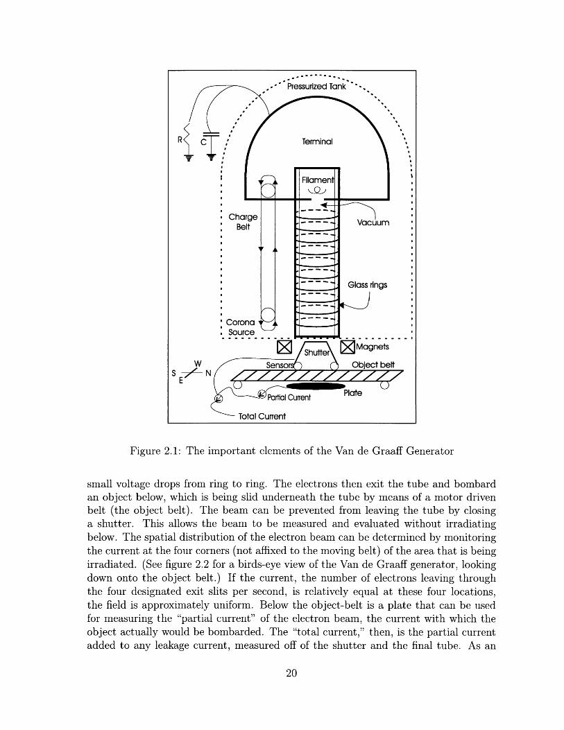
A Van de Graaff generator uses a corona source, powered by a high voltage powersupply, as its source of electrons. (Please see Figure 2.1 for a sketch of the importantelements of a Van de Graaff generator). These electrons ionize the air in the vicinity ofthe corona points so that the charge is "sprayed" onto a rapidly moving conveyor belt(the charge belt). This belt carries the charge up to an isolated high voltage terminalthat is in a pressurized environment (SF 6 gas) that helps prevent it from breaking downthe gas and "sparking". This belt introduces an inherent delay in the system that isthe height of the belt divided by its velocity. There are practical limitations on boththe speed of the belt and the electrons sprayed on: if the belt goes too fast there arediminishing returns due to electrons being lost to the environment, and if too muchvoltage is applied to the belt it can break or spark.

The high voltage terminal has a natural capacitance with ground. Furthermore, ithas a 1011 2 resistor running to ground. The electrons are coerced off of this terminalby means of a filament. The current flowing through the filament sets its temperature,and this serves as a coarse-adjust for electron flow: the hotter the element the moreamperage. The filament current is adjusted via a variac that is controlled from belowby a rod and motor setup. The fine-adjust for electron flow, then, comes from the biasvoltage of the filament. This can be controlled to precisely define the electron beam.Next, the electrons are accelerated in a vacuum tube, and directed and focused bymeans of the field created by magnets at the exit side of the acceleration tube. Thereare three magnets all together, a solenoidal focusing magnet that keeps the beamreasonably columnated, a north-south magnet and an west-east magnet, which havethe effect of pulling the beam in their respective directions, to aim it. The accelerationtube is lined with glass rings, to have the total voltage drop be realized as the sum of

S°-' Pressurized Tank

Figure 2.1: The important elements of the Van de Graaff Generator

small voltage drops from ring to ring. The electrons then exit the tube and bombardan object below, which is being slid underneath the tube by means of a motor drivenbelt (the object belt). The beam can be prevented from leaving the tube by closinga shutter. This allows the beam to be measured and evaluated without irradiatingbelow. The spatial distribution of the electron beam can be determined by monitoringthe current at the four corners (not affixed to the moving belt) of the area that is beingirradiated. (See figure 2.2 for a birds-eye view of the Van de Graaff generator, lookingdown onto the object belt.) If the current, the number of electrons leaving throughthe four designated exit slits per second, is relatively equal at these four locations,the field is approximately uniform. Below the object-belt is a plate that can be usedfor measuring the "partial current" of the electron beam, the current with which theobject actually would be bombarded. The "total current," then, is the partial currentadded to any leakage current, measured off of the shutter and the final tube. As an

Ws E7-N

E

- Total Current

object slides through the charge area, optical sensors are able to relate its position to

an observer.

Figure 2.2: View looking down onto the object belt from the shutter.

2.2 Overvoltage Protection

2.2.1 Problem Statement

The required measurements of this system are small currents that are read as a voltages

over a known (large) resistor. For example, all four sensor currents, the partial current,the total current, and even the terminal voltage, are all read as voltages by various

means. Due to the excessive charges that are present in this system (the terminal

voltage is typically measured in megavolts) it is necessary to protect all measurement

equipment from possible spikes. It is necessary, therefore, to design a Voltage Protec-

tion Circuit that possesses the following traits:

1. The output voltage needs to be read over a large resistor, to account for the

typically small input currents.

2. Any incoming spike should be sufficiently attenuated when viewed at the output.(By a factor of ten or greater)

3. The spike should be attenuated at all nodes of the circuit, not just a differentialoutput - to prevent any probe from seeing the spike.

4. There should be a delay between the peak of the spike at the input and the peak

of the spike at the output that is 1 ms or greater.

5. The output should settle within 100 ms.

One possible implementation of a protection scheme is presented in the following

section. It is then developed into a system that satisfies all of the above constraints.

2.2.2 Basic Voltage Protection Circuit

Interpreting the Goals

IInL Ra

+ +

Vin C1 C2 RVour

L Ra

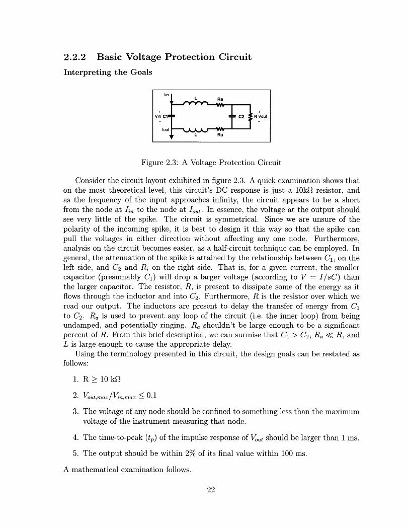
Figure 2.3: A Voltage Protection Circuit

Consider the circuit layout exhibited in figure 2.3. A quick examination shows thaton the most theoretical level, this circuit's DC response is just a 10kQ resistor, andas the frequency of the input approaches infinity, the circuit appears to be a shortfrom the node at lin to the node at Iot. In essence, the voltage at the output shouldsee very little of the spike. The circuit is symmetrical. Since we are unsure of thepolarity of the incoming spike, it is best to design it this way so that the spike canpull the voltages in either direction without affecting any one node. Furthermore,analysis on the circuit becomes easier, as a half-circuit technique can be employed. Ingeneral, the attenuation of the spike is attained by the relationship between C1, on theleft side, and C2 and R, on the right side. That is, for a given current, the smallercapacitor (presumably C1 ) will drop a larger voltage (according to V = I/sC) thanthe larger capacitor. The resistor, R, is present to dissipate some of the energy as itflows through the inductor and into C2 . Furthermore, R is the resistor over which weread our output. The inductors are present to delay the transfer of energy from C1

to C2. Ra is used to prevent any loop of the circuit (i.e. the inner loop) from beingundamped, and potentially ringing. Ra shouldn't be large enough to be a significantpercent of R. From this brief description, we can surmise that C1 > C2, Ra < R, andL is large enough to cause the appropriate delay.

Using the terminology presented in this circuit, the design goals can be restated asfollows:

1. R > 10 kQ

2. Vout,max/Vln,max < 0.1

3. The voltage of any node should be confined to something less than the maximumvoltage of the instrument measuring that node.

4. The time-to-peak (tp) of the impulse response of Vout should be larger than 1 ms.

5. The output should be within 2% of its final value within 100 ms.

A mathematical examination follows.

Analysis of the Voltage Protection Circuit

In an attempt to quantify the previous circuit, the following transfer functions were

found. During this analysis, it was assumed that the negative side of Vi/ was ground,as this corresponded to the setup used when attaining the experimental results. The

response of the circuit to a voltage over C1 is:

Volut R

Vi, 2RLC 2s 2 + (2L + 2RaRC2)s + 2RaR

This leads directly to the transfer function from Iin to Vi,:

Vn 2RLC 2s2 + (2L + 2RaRC2)s + 2RaR

Iin 2RLC1 C 2s3 + (2LC1 + 2RaRCiC 2)S2 + (2RaCi + RC1 + RC 2)s + 1

Which, in turn, leads us to the transfer function from in to Vout:

Vout R

Ii, 2RLCC 2s 3 + (2LC + 2RaRCiC 2)S2 + (2RaCi + RC 1 + RC 2)s + 1

Again, the above is true if the negative side of Vin is tied to ground. Using theabove equations, a MATLAB simulation was employed to develop (realistic) circuitparameters that meet the above requirements. By choosing C1 = .15 pF, L = .001 mH,Ra = 1 kM, C2 = 1 pF, and R = 10 kQ, the following results are conjectured by the

model. When both Vin and Vout are measured in response to an identical Iin, there will

be a 8.4:1 ratio between Vi, and Vout, there will be a delay of 1 ms until the peak ofVout, and Vout will be within 2% of its final value after .05 seconds.

Results

The circuit was constructed and given an input current via a charged capacitor, and

output voltage was recorded on a digital oscilloscope, and transferred to a computer.

Figure 2.4 shows the entire response by using an appropriately long time-frame.Note that the response is at its final value by 100 ms and that the input to output

ratio is approximately 10:1. Figure 2.5 shows the same response, only zoomed in tosee the Vot rise to its maximum value.

Note that there is a 1 ms time-to-peak in the output. Figures 2.4 and 2.5 imply that

the model has accurately predicted the response of the circuit. In fact, after feedingthe measured input voltage into the model, a direct comparison between the measured

and the predicted response can be made. As can be seen, the two plots in figure 2.6

are nearly identical. This explains the accuracy with which the model anticipated the

response goals.There is, however, one problem with this design. It does not satisfy criterion number

3 of the design goals. To see this, please examine figure 2.11. The top chart in this

figure clearly exhibits an artifact of the current spike that can be seen when referencing

a node to ground instead of differentially. The bottom graph plots the response of the

circuit that solves this problem, which is also developed in section 2.2.3.

UU

04

02 -

0

noic0 0 01 002 003 0.04 005 006 007 008 0.09 0.

time (seconds)

x 10-3

6-

0 0.01 0 02 0.03 0.04 0.05 0.06 0.07 0.08 0.09time (seconds)

Figure 2.4: The long-terminput current.

5

0

response of the Voltage Protection Circuit to a spark in

time (seconds)

0 05 15 2time (seconds)

x 10

2.5

x 103

Figure 2.5: Theinput current.

short-term response of the Voltage Protection Circuit to a spark in

2.2.3 An Improved Voltage Protection Circuit

A natural solution to this problem is to place capacitors (C3) between the positive sideof Vot and ground, and between the negative side of V0ot and ground. The capacitorwill tend to shield against a spike by "integrating" it out over time. A capacitor valueof 1 pF is chosen to keep the RC time constant (RC3 = 10 ms, well below our settling

0.1

0

0 0.

0n

x 108

7

6-

5 A

2

1 i

-10 0.01 0.02 0.03 0.04 0.05 0.06 0.07 0.08 0.09 0.1

time (seconds)

Figure 2.6: Predicted and actual responses of the Voltage Protection Circuit

time requirement of 100 ms) manageable. Figure 2.7 shows this improved circuit, withparameter names replaced with their respective values in this implementation.

Figure 2.7: An improved voltage protection circuit, with parameter values.

Analysis of the Improved Voltage Protection Circuit

The math for this circuit is considerably more in depth than the previous circuit. Asin the last case, we assume that the negative side of both C3 's is grounded to the sameground as the node that provides Iot, as this was the experimental setup used forverification. Unfortunately, using this setup removes symmetry from the circuit, andwith it the easy half-circuit analytic method. The transfer function from Vmj to Vot isrelatively easy to find, but the other two transfer functions (lin to Vi and Iin to Vout)are much more algebra-intensive. To solve them, the symbolic mathematics packageMaple was used. The results were used in the model (see section 2.2.3, but are toolong to publish in closed form here. (The denominator is fifth order.)

From Vin to Vt we have:

Vout R

Vi (2LRC2)s 2 + (2L + 2RaRC2 + RaRC 3)s + 2Ra + R

Please note that the negative side of Vi, is grounded in the above equation, due to theexperimental setup. When used in its final application this circuit will be placed inseries with the rest of the system.

Results

As before, the circuit was built and given a spike in I,,n via a charged capacitor. Theoutput (Vt) was recorded on the digital scope and transferred to a computer. Thecircuit's response is shown here, in a similar fashion as before. Figure 2.8 displays theentire response, by using a large time-step. Figure 2.9 is the same circuit (differentinput, as can be noted by comparison), only with a smaller time step to see the risetime.

40

30-

S20

10-

0

0 002 0.04 006 008 01 012 0.14 016 018 0.2Time (seconds)

4

3

2-

1

0

-10 002 0.04 006 008 01 012 0.14 016 0.18 02

Time (seconds)

Figure 2.8: The long-term response of the Improved Voltage Protection Circuit to aspark in input current.

The results are similar: this circuit also has an approximate 1 ms time-to-peak inthe output (perhaps longer!), the response has settled well before 100ms, and there isa ratio of approximately 10:1 from the input to the output. Furthermore, the modelused to predict the response of this circuit is very accurate. It is almost difficult to seethe difference between the theoretical and measured results in figure 2.10. The thinline (theoretical results) barely deviates from the noisier measured results.

40 -

2

0

-200 0.001 0.002 0.003 0.004 0.005 0.006 0.007 0.008 0.009 0.01Time (seconds)

Figure 2.9: The short-term response of the Improved Voltage Protection Circuit to a

spark in input current.

2.2.4 Comparison of the original Voltage Protection Circuit3-2-

and the Improved Voltage Protection Circuit

It is fair to say, then, that this circuit performs at least as well as the original VoltageProtection Circuit, even with the added capacitors. The final test is to see if there is amarked improvement protection against spikes at the other nodes. Namely, the voltagefrom the positive side of Vot to ground shouldn't spike as it did for the previous circuit.Figure 2.11 shows a direct comparison of this voltage in the original circuit (the darkerplot) and in the improved circuit (lighter plot). As can clearly be seen, the spike thatwas present in the original circuit has disappeared. This circuit, then, is suitable foruse in protecting the computer equipment from possible spikes from the Van de Graaffgenerator.

2.2.5 Final Implementation and Improvements

Of course, if the circuit is hit with a very large surge, something will give. Somecomponent will overload, burn out, or otherwise fail. To help prevent this, an extrasafeguard can be taken by placing passive "surge suppressor" components across theinput and output terminals of the protection circuit. This surge suppressor is essentiallya very nonlinear resistor that shorts in the presence of excessive voltage. To remainpractical, 18 volt surge suppressors are used - any voltage above 18 volts is deemedexcessive. In its final form, the circuit can be made in a layout such as the one infigure 2.12. Note that this layout uses the actual size of components.

There are a lot of engineering decisions involved with the layout in figure 2.12.

3.5 -

2.5

2

1.5 -

1-

0.5

0 0.001 0.002 0.003 0 004 0.005 0.006 0.007 0 008 0.009 001Time (seconds)

Figure 2.10: Predicted and actual responses of the Improved Voltage Protection Cir-cuit.

For instance, note the spacing between the input terminals. They are placed close sothat in the case of a very large spike it will actually break down the air between thetwo terminals and spike through the circuit - showing no effect at the output. Thereis a gap between the high voltage and low voltage sections of the circuit to preventcrossover between these two sides.

2.3 Magnet Control

2.3.1 Problem Statement

During the irradiation of an object, it makes sense (for efficiency, predictability, andreproducibility's sake) to maximize the amount of the beam that hits the object. Inother words, provided a terminal voltage we must maximize the strength of the beamthat hits the object. There are three different ways to measure this beam strength.One (the direct method) is to use the partial current, the number of electrons persecond that arrive on the circular disk underneath the object-belt (see figure 2.2). Apotential problem may arise, however if the object is thick; not allowing any electronsthrough the object (much less the object belt). Another is to use the four nano-amperesensors that are located in the northwest, northeast, southwest, and southeast cornersof the radiation area. It has been experimentally shown that when the partial currentis maximized so is the sum of the four sensors. These four sensors also need to read(approximately) equal values, in order to assure that the beam is distributed evenly onthe radiation area. Finally, the total current (see figure 2.1) can be used as well. It isimportant to note that there is the potential of a physical coupling between the steering

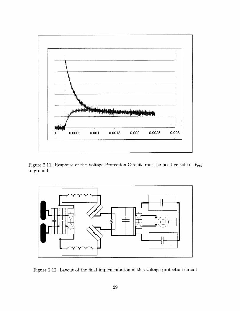
Figure 2.11: Response of the Voltage Protection Circuit from the positive side of Votto ground

Figure 2.12: Layout of the final implementation of this voltage protection circuit

magnets. The columnating magnet could interfere with the north-south magnet, andlikewise with the west-east magnet, or vice-versa. Currently the following manualprotocol (as developed by Ken Wright, MIT High Voltage Research Lab) is used tomaximize the beam current:

1. Fix the energy (the charge belt current) that the Van de Graaff generator will beusing.

2. Adjust the solenoidal magnet until the partial current is maximized.

3. Adjust the N/S magnet until the partial current is maximized.

4. Adjust the W/E magnet until the partial current is maximized.

5. Adjust the solenoidal magnet once more.

It has been observed that the magnet settings vary both with beam energy and withbeam current (which is proportional to the filament temperature). Another potentialproblem is that the acceleration tube is made out of glass, and could take on a chargeover time, which may introduce "second-order" dynamics. If a model of the systemcan be derived, this protocol can be forgone, by setting the magnets at their propervalue and then allowing the system to warm up to them.

2.3.2 Observations and Assumptions

This section is an attempt to provide the reader with an intuitive feel for the response ofthe Van de Graaff generator to various inputs. There are a lot of variables, dependen-cies, and conclusions drawn in the rest of this section which are based upon this "feel",and it is of benefit to the reader to have some understanding of these non-obviousconclusions before continuing. This section is non-rigorous and non-mathematical.

For the purposes of this paper we have full control of the current in the north-southmagnet (is), the current in the west-east magnet (ie), the current in the solenoidalfocusing magnet (if), and the terminal voltage. We do not have complete control ofthe filament temperature, which determines the total current (itotal) and the partialcurrent (ipatial). Current flow (by means of the filament) depends on a temperaturegradient, and the temperature varies during an irradiation. Provided no other changes,however, the total and partial current move proportionally. That is, the ratio betweenpartial and total current remains approximately constant with variations in temper-ature. Figure 2.13 shows a set of data that exhibits this ratio. Unfortunately thisratio breaks down at lower temperatures, as there is less current flowing through themachine and therefore fewer electrons are lost to the surroundings.

Figure 2.13 also raises another issue. It is assumed throughout this paper that thesum of the four directional nano-ampere sensors is as good (perhaps better) a metricfor representing the beam in the irradiation area as the partial current. Logically,there are a number of arguments for this. A sense of beam dispersion can be obtained

Sum / Total and Partial / Total for various FilamentTemperatures

0.7

0.6

0.5

. 0.4 = =_ Partial/Total

S0.3- - Sum/Total (Scaled)

0.2

0.1

0 5 10 15 20 25

Total Current (representation ofTemperature)

Figure 2.13: The Ratio of Sum of the four direction sensors divided by total current,and partial current divided by total current for an adjustment in filament temperature.

through the four sensors which is not seen in the partial current. Also, the partialcurrent plate is located underneath the object belt, so lower energy electrons may notbe able to penetrate the belt (or at least to the extent that they would at higherenergies), whereas the four sensors are above the belt, avoiding this problem. To seean initial "proof' that the sum of the four sensors can at least replace the partialcurrent measurement, please examine Figure 2.14. It is evident that the sum currentis proportional to the partial current. Although this proportionality changes withterminal voltage (perhaps representing the amount of energy absorbed by the objectbelt) it is still a linear relationship.

When examining the output of the Van de Graaff generator, there is one optimalsetting of in, iwe, and if for each terminal voltage. By optimal it is meant that theratio of partial current to total current (or for that matter the ratio of the sum of thefour directional sensors to total current) is maximized, and the beam is distributedevenly over the irradiation area (as determined by the four directional sensors). Thereare, however, plenty of local maximums and minimums over the set of possible inputcurrents, which present a notable algorithm development problem.

If we place the system at its optimal point (as determined by the manual method

Sum vs Partial

Figure 2.14: The Summed Current versus Partial Current.

described in the introduction) and vary the magnet currents one at a time we see theresponse (the ratios) taper off as the current leaves the optimal point in either direction.Put most simply it looks like a parabola. This is true for all ins, iwe, and usually truefor if. The focusing current has the peculiarity that, at low terminal voltages, as ifgoes to 0 (leaving the optimal point going to the "left") the response gets stuck at aconstant level. (It bears a strange resemblance to the bode magnitude plot of a second-order low-pass filter.) It has been assumed that this is due to hysteresis in the focusingmagnet (the magnet has been driven with only positive current for as long as it hasbeen in operation) such that as the current goes to zero there is still a magnetic fieldpresent strong enough to affect beams that have relatively little energy. Regardless, allother settings look roughly parabolic, influencing decision to use a second order fit forthis system.

As we change the terminal voltage, a large non-linearity (that will be addressedlater) is introduced into the system. Despite this, though, it can be said that themagnitude of i,,, iwe, and if at the optimal point move monotonically with terminalvoltage. How they move may vary from day to day (as is shown in the set of data),but it is the observation of those who run this system daily that on a given day thenecessary currents to optimize the system increase with terminal voltage. Please see

3 35 4 45 515 2 25

partial

0 05

section 2.3.6 later in this section for a more detailed discussion of this.Lastly, it is a basic assumption in this paper that the effect of the glass rings taking

on a charge during operation (and thus affecting later results) is minimal and not worthtaking into account. To test this assumption two runs of the machine were performedat a terminal voltage of 1.5 MV. In between these runs, the machine was operated for aprolonged period at a significantly higher (greater than 2.5 MV) terminal voltage. Theresults of the two 1.5 MV results are presented in figure 2.15, and are nearly identical.

Figure 2.15: The effect of the glass rings taking on a charge is inconsequential.

2.3.3 Modeling

While a state-space model for this system could potentially be used, in terms of imple-mentation such a model is entirely unnecessary. The generator is controlled via dataacquisition and output hardware interfaced to a computer with a GPIB bus. Laten-cies within the computer, the bus, and the acquisition hardware entail that the entiresystem cannot operate at speeds much greater then 1 Hz. Any intermediate variablescan be assumed to arise from phenomena that are orders of magnitude faster, and havereached their steady-state values by the time the next data acquisition cycle has beenperformed. For this reason, a simple input-output coupling matrix model has beenassumed for the purposes of this analysis, which is of the form:

A Comparison of Two Runs at 1.5 MV, Separated by aProlonged Run of Higher Terminal Voltage.

251

15-#+-Total Current Run #1--- Partial Current Run #1

-&-Total Current Run #2- -Partial Current Run #2

10

5

various (identical for both runs) settings of the three directional magnets

y = Ax

The output vector will simply consist of the outputs available to us:

1 inw

Y2 ine

Y3 isw

Y4 ise

Y5 itotal

Y6 J i partial

inw is the current measured off of the north-west nano-ampere sensor.ine is the current measured off of the north-east nano-ampere sensor.i , is the current measured off of the south-west nano-ampere sensor.ise is the current measured off of the south-east nano-ampere sensor.ipartial is the partial current as defined in the introduction.itotal is the total current as defined in the introduction.

The input vector will consist of the variables over which we have direct control (i.e.filament temperature is excluded). We will also be including second order terms forthe inputs in accordance with the notes made in the observations section. So:

i2X1 ns

X2 insi2X3 we

X = X4 we

X5 focus

X6 ifocus

x 7 C

ins is the current through the north-south magnet.iwe is the current through the west-east magnet.ifocus is the current through the focusing magnet.C is the combined DC term of the three inputs.

The coupling matrix, A, will then consist of coefficients that match the inputs tothe outputs. These coefficients are assumed to be functions of primarily the terminalvoltage. i.e.

all11 " a17

A=a 61 a 67

where aij = f(terminal voltage).

2.3.4 Modeling for fixed Terminal Voltage

Theory

The use of the coupling matrix for a given terminal voltage, At.v., will be to determinethe initial optimal operating point for that terminal voltage. Ideally, the characteristicsof the Van de Graaff generator are fixed, and once a coupling matrix is determined, itwill hold for all time. In reality, the generator's characteristics vary greatly from dayto day depending on innumerable conditions, such as changing sensor locations, tankpressures, vacuum pump efficiencies, room temperatures, and the vacuum tube poweramplifiers used for setting the filament temperature. Because of this, a more realisticapproach is to start at a guessed optimal point, conduct iterations around this point,use recursive least squares to update the coupling matrix At,., and then find the trueoptimal point du jour.

Having a decent guess for the initial optimal point is vital for a quick convergence.Therefore, the hope is that a general coupling matrix A can be obtained, where eachcoefficient, aij, is a function of terminal voltage. The constant coefficients of thecoupling matrix of interest, At.,., can then be obtained for any given terminal voltageby simply evaluating the general coupling matrix coefficients at a set terminal voltage.The initial optimal point can then be obtained from this first guess of At.v..

In order to obtain A, several different At.v. matrices will be obtained, and then,hopefully, the coefficients of the general matrix A can be formed by fitting curves

(non-linear if necessary) to the coefficients of the At.,.'s. To accomplish this, sets ofoutput and input measurements were taken around optimal points obtained from themanual method described in the introduction at several different terminal voltages (0.5,1.0, 1.5, 2.0, and 2.5 MV).

For each of the sets of data, the coupling matrix At.v. was obtained as follows. Theinput and output data could each be combined into stacked input and output vectors.

y(1)- ...- yi(k)

" ; . [y(1) y(2) ... y(k)

Y6 (1) ... Y (k)

and

x (1) x, X l(k)

-- - . [""x(1) x(2) ..- x(k)]F xi(1) ... x (k) 1

such that

= At.v.X

and k is the number of points taken in the set.Now we'd like to find the coefficients of At.v.. This is not quite the normal least

squares problem, as usually we're trying to find the vector x, not the matrix At.v.. We

can transform this into the familiar form by taking the transpose of the last equation,so that:

y' = (A)' = A'

the solution of A follows as:

A=

which can be re-written as

by noting that

Results and Discussion

The input and output data from the different runs at different terminal voltages were fitto coupling matrices in the least squares sense. The results are shown in the followingfigures.

Figure 2.16: Various responses at 0.5 MV Terminal Voltage.

As is easily seen from Figures 2.16-2.20, the model that uses the previously men-

tioned least squares technique fits the experimental data well. A more specific discus-sion of the figures follows.

XVI Focus Magnet around optimal point 8 X W-E Magnet around optiml point8 8

1 6

2 Actual DataComputed Data

0 0.2 0.4 0.6 0 20 40 60 80kocus current (locu) wea-east magnet current (iwe)

x Ytf magn-s r e wound opmu pont8

s16

32

0-100 -50 0 50

Noh-South magnet current (Ins)

Vuhingthe Focus Magnt ound opt point

0 0.5 1focus curent (hoa)

Vwyhg the North-Souh magnet wound optlm polin0.03,

VmyingitisWsst-E~ Mspisi misid oplinisi poliOVvig the We-Ert Magnt wound opml point

0.03

0.02

0.01

0-50 0 50 100

wst-as agn currnt (kn)

00 -50 0 50North-South magnet cuent (is)

Figure 2.17: Various responses at 1.0 MV Terminal Voltage.

Varying he Focus Mgn around optinsl point Vying the West-Est Magnt ound opl point0.05 0.05

S0.04 0.04

S0.03 0.03

0.02 0.02

C 0 .01 -n 0 .0 1

0 0.0 0.5 1 1.5 -50 0 50 100 150

tocus cumrnt (fou) Varying the West-East magt wh ocusing too high

Varing the North-South magnet ound optimal point 0.050.05 0

-0.050.04 -50 0 50 100

West-East magnet current (ins)

10.03

0.02 Varying the North-South magnet with focusing too high0.05

0.01 0

-0.05-100 -50 0 50 -100 -50 0 50 10050 -100 -50 0 50 No-Sh magnet current (nrs)

Norl-South mgnet currnt (ns)

Figure 2.18: Various responses at 1.5 MV Terminal Voltage.

Figure 2.16: While the north-south and west-east predictions are very close, the fo-cusing magnet prediction misses the target. This can be attributed to the lackof a parabolic shape in the real data. As mentioned before, the focusing magnetseems to have hysteresis that affects low energy beams.

Figure 2.17: Again, the north-south and west-east predictions are close, but the fo-cusing magnet prediction is much closer then before.

Vinithiothe Focus Magnet wound opihotet point Vayingihe West-East Magnet wound optinul pobWVying the Focus Magme around opTM pnt

0.04

0.03

0.02

0.01

0

-

0 0.5 1 1.5focu urrent (Ilocus)

Varyg th North-Souh magnet wound optimal por0.04

0.03

0.02

0.01

-100 0North-ouh magnat urrent (in)

Figure 2.19: Various responses

Varying th Focus Magnet around optimal point

0.5 1 1.5focu current (idcus)

varyng the North-South magn around optrnal point0.04

0.03

0.02

0.01

-L -100 0 100North-South magnat current (In )

Vwryig h WW-Ea Magne round optimal point0.04

0.03

0.02

0.01

0-50 0 50 100 150Vary the Wet-Eat magn wth focusing too high

0.04

-50 0 50 100 150West-East magnet cuent (ina)

Varying the Norh-South magne with focusing too high0.05

-0.05-100 0 100 200

North-South magnet curent (ins)

at 2.0 MV Terminal Voltage.

Varying the West-East Magnet around optimal point

-100 0 100 200wes-east magnet current ()

Varying the North-South magne with focusing too high0.04

0o.o03

0.02

0.01

-?00 0 100 200Nor-South magna curnrent (Ins)

Figure 2.20: Various responses at 2.5 MV Terminal Voltage.

Figure 2.18: This time we see an improvement in the focusing magnet prediction,but the north-south prediction is off. Although it (approximately) guesses theappropriate optimal current, the predicted magnitude of the response isn't ac-curate. The 1.5 MV set of data was actually taken on two different days, andended up having vastly different optimal north-south magnet currents, hence thediscrepancy. Note that the 1.5 MV data does a fairly good job of predicting datathat is not near the optimal point as well. It is the expectation that the model

should be "close" in these ranges, but an exact match isn't necessary as we willbe using this model to predict the neighborhood of the optimal point.

Figure 2.19: Again, acceptable fits all across the board, especially when consideringusing the At.v. matrix to pick out the location of the optimum point.

Figure 2.20: The fits to the data in the vicinity of the optimal point are good, butthere is a serious degradation of the data when looking outside of this optimalpoint. It does however, match the appropriate range of values when the focusingcurrent is set too high, it just shifts the peak slightly.

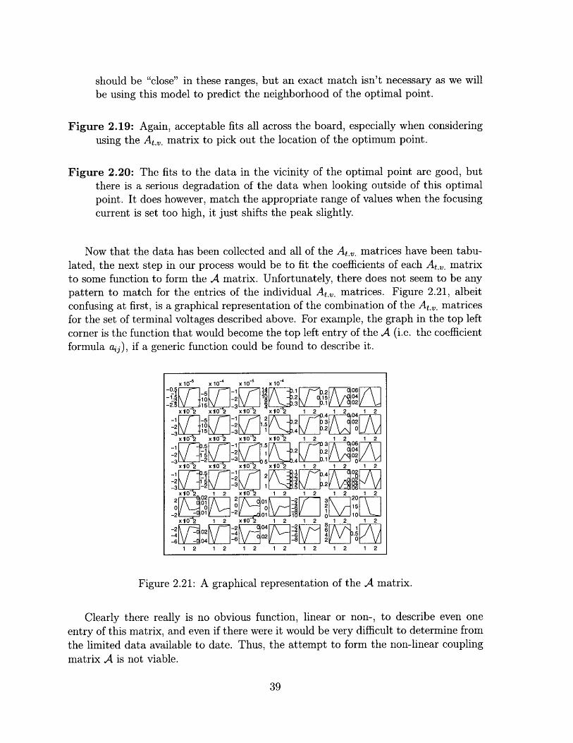
Now that the data has been collected and all of the At.v. matrices have been tabu-lated, the next step in our process would be to fit the coefficients of each At.,. matrixto some function to form the A matrix. Unfortunately, there does not seem to be anypattern to match for the entries of the individual At.'. matrices. Figure 2.21, albeitconfusing at first, is a graphical representation of the combination of the At.,. matricesfor the set of terminal voltages described above. For example, the graph in the top leftcorner is the function that would become the top left entry of the A (i.e. the coefficientformula aij), if a generic function could be found to describe it.

x 0l x 10-4

x 10-s

x 10-0 2x10 106

x102 x2 x102 x02 1 2 12 1-2 _ 10 5 J]_ _3 _L 2 _ . 32

1 O 2

x-1 2 x10-2 xlO 2 xo 2 1 2 1 2 0 1 2

x10-2 xlO-2 xO-2 x1 2 1 2 1 2 1 22 3 206

-2 E I2 5_ 01 1[ r.2 10 --]

- 1 2 0 01-22 I 15

xo 2 x10 2 xO 2 x102 1 2 1 2 1 2

-- 1 3 2 64-2 5 2

x10 2 1 2 x102 1 2 1

-2 0 - 04_T 772]

1 2 1 2 1 2 1 2 1 2 1 2 1 2

Figure 2.21: A graphical representation of the A matrix.

Clearly there really is no obvious function, linear or non-, to describe even oneentry of this matrix, and even if there were it would be very difficult to determine fromthe limited data available to date. Thus, the attempt to form the non-linear couplingmatrix A is not viable.

2.3.5 Modeling over all Terminal Voltage

Theory

Another attempt at modeling the system was made, this time using brute force. Sincecreating coefficients that were functions of terminal voltage didn't work, our next at-tempt was to include the terminal voltage as an input into the model. The new modelfor this system would then be:

y = Ax

A is a general coupling matrix relating the input x to the output y. This matrix couldthen be used to pick the initial optimal point for a given terminal voltage from whichthe recursive least squares of the matrix At.v. would start. The input vector, x, in thiscase would be:

.2Xl ns

X2 ins.2

X3 'we

X4 iwe

X5 if ocus

X6 ifocus

x7 T.V.

x8 C

where T.V. is the terminal voltage of the Van de Graaff, and all the other entries are thesame as before. The output vector, y, is the same output vector as was used previously.

The data from the various runs were then stacked into input and output matrices,and the coupling matrix A was fitted to the data in a least squares sense in the samegeneral manner as before.

Results and Discussions

The performance of the coupling matrix A is compared against the actual data inFigures 2.22-2.24. A discussion follows.

Figure 2.22: These six graphs show that the general coupling matrix model actualperforms surprisingly well for our purposes. Although the magnitudes of the fitscan be off by as much as fifty percent, the location of the peaks of the fit, theimportant issue to us, corresponds quite well to the actual data.

Figure 2.23: Again, in terms of actual magnitude, the fits are significantly off fromthe actual data. The peaks, however, are acceptable although this time they arenot as closely correlated to the actual data peaks as in the west-east magnet case.The important thing to note is that even in the worst case of the peak being off(T.V. = .05), the calculated peak is still within the broad peak area of the actualdata.

Vaulyg h We*Ema IMhtnd opmal pot TWO50.01

0.005

0 20 40 60 80

Vyig th Wms..mt M mmd apmkd pon V-1.5 DOy

0.00

0.04

0.02

50 0 50 100 150

-50 0 50 100 150wampmuina=uwh)

0

Vm~dne r Wet.-as apet amMd Qopml putt TV .o0.03

0.02

0.01

0-50 0 50 100

Vawyk Wge-s Maulp amsmmd pok iTV-.1A Day 2

arig Vm WeEat MawdWamumd opm poht TIV.0.04

0.02

-o 0 100 200wsutmasnt rouriWm)

Figure 2.22: Comparison of the actual data and the computed datamatrix A for the west-east magnet and several terminal voltages.

Figure 2.23: Comparison of the actual data and the computed datamatrix A for the north-south magnet and several terminal voltages.

from the general

from the general

Figure 2.24: These graphs show that the general coupling matrix idea performs quitepoorly when compared to the actual focusing magnet data. In terms of fittingthe actual magnitudes, the performance is a little worse than in the north-southand west-east magnet cases. However, in terms of getting the peaks right, themodel really starts to fall apart. At the higher terminal voltages, the calculated

Vasing m Foam Mn amd opdI point TV.5 VMying I Fou -M ammud opnal point TV-.

Vaying t Focus Ma t a d o p point TV-1.4 day I Vayingr Fou M.p amd op"l pok TV-.1. day 2

0.06 0.04

0.02

0 0.5 1 1.5 0 0.5 1 1.5

Voymg F Focus Mwet aroud op l poin TLV.O Vaying Focus MapIm amd opuimd okrTV-2.5

0.04 0.050.04

S0.02-0.03

0 0.5 1 1.5 0.5 1 1.5foammit curran obou

Figure 2.24: Comparison of the actual data and the computed data from the generalmatrix A for the focusing magnet and several terminal voltages.

peak is fairly close, but as the model moves into the lower terminal voltages, thecalculated peak is no longer within the broad actual data peak.

Overall, using the general coupling matrix, A, does not seem like it will be a viableoption for picking an initial optimal point for the system. While the fit performsdecently well compared to the actual data for the north-south and west-east magnets;the performance to the actual focusing magnet is simply too far off to justify thismethod. This method could conceivably be used in practice, but a more efficientmethod is desirable.

2.3.6 Picking Optimal Points

Since the last method did not work well for predicting the optimal point at any specificterminal voltage, we are still stuck deriving a method whereby this optimal point canbe determined. The knowledge that we have gained from the previous sections of thispaper will allow us to do this easily. We will make use of two related facts for thismethod. The first is that when examining two proximal terminal voltages, the At.,.matrix from one can be used to approximate the other. Figures 2.25 and 2.26 exemplifythis.

The other useful observation is that to a good approximation the optimal pointsvary monotonically with terminal voltage, as presented in the observations section. In

fact, a simple linear fit comes reasonably close to this data, as shown in Figures 2.27

through 2.29.Using this knowledge, the final algorithm will follow this general plan:

Figure 2.25: Graphs showing T.V. = 1.25 MVand the fits from the T.V. = 1.0 MV and the

Figure 2.26: Graphs showing T.V. = 1.75 MVand the fits from the T.V. = 1.5 MV and the

data along with a fit to that set of data,T.V. = 1.5 MV data sets.

data along with a fit to that set of data,T.V. = 2.0 MV data sets.

1. Fix the terminal voltage of the Van de Graaff generator.

2. Compute the optimal point for that terminal voltage by plugging the value intothe linear fit of the actual optimal points.

3. Pick the closest At.,. matrix to that terminal voltage. Previous At.,.'s are stored

Varyingth Focus Magne round opil point Varying the West-Est Magnet mund opreal point0.04 0.04

0.03 0.03 , ..

O.01 I-iactu ! aI 10.01

0 00 0.2 0.4 0.6 0.8 -50 0 50 100

focuscurrent (locus) wet-east n cunt ()

Vayingthe North megne around optn point0.04

S0.02

50 -100 -50 0 50Noth-South maet curmnt (in )

Varying the Focus Magne round optimrapo Varying the Wed-East Magnet round opdmW point0.05 0.04 - -

0.04- 0.03

a0.03 0.02

10.02 - 0.01 V0.00

Ea u 0

0 -0.010 0.5 1 1.5 -50 0 50 100 150

focus current (ocus) west-east mgnet currnent (i)

Varying the North-South magnet round optmnl point0.04

0.03 , -

0.02

0'

-00 -100 0 100North-Soulh magn currt (Ins)

Optimal Iwe for different Terminal Voltages

60

50 = 11.81x + 17.286R = 0.789

"40E

SOptimal Iwec 30

- Linear (Optimal Iwe)

0 20

10

00 1 2 3

Terminal Voltage (MV)

Figure 2.27: Optimal points for Ie versus Terminal Voltage.

on the computer.

4. Use this At.v. matrix to initiate a recursive least squares fit, starting with datapoints around the initial optimal points derived in step 2.

5. Keep generating data points with the Van de Graaff generator extending aroundthis initial data point until a new optimal point can be identified.

6. Set the Van de Graaff generator at this optimal point for the duration of theexperiment.

7. Save the computed At.v. matrix and the optimal point for this terminal voltagefor later use.

2.3.7 Similarity Transform Observations

Since many of the inputs and outputs of the modeled system (i.e. the north-south andwest-east magnets, and the northwest, southwest, southeast, and northeast sensors)are directional in nature, it may prove interesting to look for patterns in the A matrix.We would not expect to see any patterns as is, because the coordinate directions of

Optimal Ins, for different Terminal Voltages

70

60 = 10.19x + 29.339R2 = 0.2983

50

E 40--- Optimal Ins

3 - Linear (Optimal Ins)

20

10

00 1 2 3

Terminal Voltage

Figure 2.28: Optimal points for Ins versus Terminal Voltage.

the outputs of the system do not match the coordinate directions of the inputs. To getaround this problem, we make use of a similarity transform, changing the directionaloutputs from northwest, southwest, southeast, and northeast, to north, south, west,and east. i.e.:

north component

south component

west component

east component

total component

partial component

.5(inw + ine)

.5(is, + ise).5(inw + isw).5(ine + ise)

itotal

ipartial

where T is the similarity transform of interest.

We can multiply our model by this T to obtain a new coupling matrix, TA, whosestructure, if we assume orthogonality between the north-south and west-east magnets,can be expected to follow the form:

y

inw

ine

is,

ise

itotal

L ipartial

STy

Figure 2.29: Optimal points for If versus Terminal Voltage

* = Ty = YAx =

north component

south component

west component

east component

total component

partial component

indicates an expected entry in the coupling matrix.indicates an expected 0 in the coupling matrix.indicates no expectations for that coefficient in the coupling matrix.

To test out this similarity matrix, the 2.5 MV data was first normalized. Thisnormalization was done so that the coefficients of coupling matrices could be directlycompared. A coupling matrix, A 2.5*, was then fit to this data and multiplied by T.The result was:

Optimal If for different Terminal Voltages

1.4-

1.2 0.4914x - 0.03841.2 R2 = 0.9734

EE0.8 --.- Optimal If0.6 --Linear (Optimal If)

o 0.4

0.2

0

0 1 2 3

Terminal Voltage (MV)

0 00 00 0

.2ns

insi2we

'we.2f

ifC

-0.0771 0.0162 -0.2389 0.4308 -1.5127 2.4522 0.2434-0.0677 0.0822 -0.2395 0.4376 -1.2396 2.2243 0.0906-0.0745 0.0475 -0.2562 0.3844 -1.3687 2.2792 0.3015

Ty = TA 2.5 xZ TA2.5* = -0.0745 0.0509 -0.2221 0.4840 -1.3836 2.3974 0.0325

-0.0005 0.0054 -0.0078 0.0169 -0.1170 0.2265 0.8855-0.0749 0.0568 -0.2438 0.4348 -1.2440 2.0951 0.2787

Recall that the output and input vectors are composed of:

yi north current xl (north-south magnet)2

Y2 south current x 2 north-south magnet

Y3 west current x 3 (west-east magnet) 2

Y4 east current as inputs and x 4 west-east magnet as outputs.Y5 total current x5 (focus magnet)2

Y6 partial current x 6 focus magnetx7 constant

There are a couple of things which can be said about this matrix (TA 2.5*).

* Looking at the row which determines total current (row 5), we see that thisoutput is determined primarily by the constant term (column 7). Intuitively thismakes sense, as the current should be set primarily by the speed of the Vande Graaff generator's belt and partially by the terminal voltage the generator isoperating at.

* We see that the partial current (row 6) has a stronger dependence on the focusingmagnet (columns 5 and 6) then the other inputs. Again, this makes sense. Thepartial current sensor has a large surface area, and will depend primarily whetherthe beam coming down the tube is focused rather then if the beam is a little tothe north, south, west, or east.

* Finally, there is no obvious relationship between the directional outputs (rows 1-4), and the directional inputs (columns 1-4). This is because there is a verysmall range over which, for example, an increase in the north-south magnet willcause an increase in the north current component, a decrease in the south currentcomponent and no change in the west or east current components. Outside ofthis range, an increase in the north-south magnet will cause decreases in thenorth, south, west, and east current components as the electron beam begins tolose current to the metal sides of the acceleration tube.

To show that there is a range over which the north-south magnet primarily affectsthe north and south currents, a linear fit was made to data from the linear range of theTV = 2.5 MV run. Again, this data was normalized to itself so that the coefficients

of the transformed matrix could be directly compared. To highlight this point, thefocusing magnet was not taken into account and the north-south and west-east magnetswere assumed to be linear. So:

yl north current {xz (north-south magnet)2

3 wesouth current as inputs and x2 north-south magnety3 west current x3 (west-east magnet)2

Y4 east current X4 constant

and the transform:

.5 .5 0 00 0 .5 .5.5 0 .5 00 .5 0 .5

was used. The resulting TA2.5** matrix from this fit was then:

-0.0050 0.0040 1.0010-0.0372 -0.0012 1.0384-0.0195 0.0775 0.9420-0.0227 -0.0746 1.0973

This matrix shows that, over the linear range:

* The east current component (row 4) depended primarily on the negative of thewest-east magnet (column 2).

* The west current component (row 3) depended primarily on the west-east magnet(column 2).

* The south current component (row 2) depended primarily on the negative of thenorth-south magnet (column 1).

* And it's anyone's guess what is going on with the north current component(row 1).

What these results do show us, though, is that the coupling between the differentinputs and the different outputs are often non-intuitive over the entire range of thebeam. This might explain why previous attempts to model the system from a physicalstandpoint met with failure. The results also show that, over a small range near theoptimal point, the directional inputs can be expected to affect the directional outputsin a somewhat predictable manner.

Chapter 3

Application: System Structure

A few words about implementing this proposed control scheme are included for here.

3.1 External Interface Issues

* All information will be shared between the instruments and a concentrator viaa GPIB network using the IEEE 488.2 communication protocol, to insure thatall instruments will be safe from the dangerous voltages present in the Van deGraaff. Instruments that use the RS-232 or RS-485 communication protocol willalso be used, but will still communicate with the computer over the GPIB bus,by means of a serial-to-GPIB converter.

* The north-south and west-east magnets will be current driven to avoid hysteresis.The approximate range of currents needed to drive these magnets is -100 mA to100 mA, at a resistance of approximately 40 Q. That is, the current source neededto drive this must be able to operate in a constant current mode, that can outputup to 100 mA at up to 4 Volts. There are 0-20 mA current sources available forRS-485 that when appropriately biased and amplified will work in this range.

* The focusing magnet, on the other hand, requires some special instrumentation.It operates in a range of 0-2 Amps, at up to 200 Volts. For this application, ahigh current/voltage power supply (capable of 0-7 Amps at 300 Volts) that isanalog programmable will be used. The analog programming will be performedby a GPIB compatible D/A converter that can create a very accurate and fastsettling 0-1 Volt output. This output will serve as the analog input to the highvoltage power supply, which will in turn drive the focusing magnet.

* The four beam-position currents (inw, i s e, i, i), the terminal voltage, the

partial current, and the total current are all read through a Keithley 8 channelvoltage scanner, after being scaled into range by appropriate resistor networks

(or in the case of the terminal voltage a generating voltmeter).

* At present, the system is also capable of reading data from a slew of other in-struments, including the Analog Devices 6B serial products (read voltage, setcurrent, read RTD, read/set 32 bits of digital logic), and Tektronix 200 and 500series oscilloscopes.

3.2 Data Processing within the Concentrator

Figures 3.1 and 3.2 show pictures of the working concentrator and observer. All codewas written in LabVIEW 4.1, and is portable to any system that has LabVIEW com-piled for it; no platform dependent operations were used in the design of this project.Figure 3.1 is a hierarchy of the concentrator. Consider each square a functioning pro-gram on the computer. A line connecting two programs indicates a data dependency.The box marked "conc" is the part of the concentrator that is running immediatelyat startup, the part that receives data over the network. This part of the code runsbefore a parameter file has been downloaded from an observer. The remaining boxeson the top row are all processes that are loaded by the parameter file. They are (fromleft to right):

* Set HP Voltage. This process is used to control the focusing magnet by meansof a GPIB programmable voltage supply which is connected to a large (analogprogrammable) current supply.

* Set Analog Devices 6B21 Current #1. This process sets a current of 0-20 mAwhich can then be used (through proper amplification) to control the north-southmagnet's current.

* Set Analog Devices 6B21 Current #2. This process is used to control the west-east magnet's current.

* Local Startup process. This process initializes the instruments for which thisparticular concentrator is responsible.

* Partial Current. This process monitors the Partial Current from the KeithleyScanner.

* Scan Channels 1-4. This monitors inw, ine, is, and ise by means of the KeithleyScanner.

* Terminal Voltage. This process monitors the Terminal Voltage from the KeithleyScanner.

* Total Current. This process monitors the Total Current from the Keithley Scan-ner.

The processes in the second row all are subroutines of the startup concentratorprogram. From left to right they are:

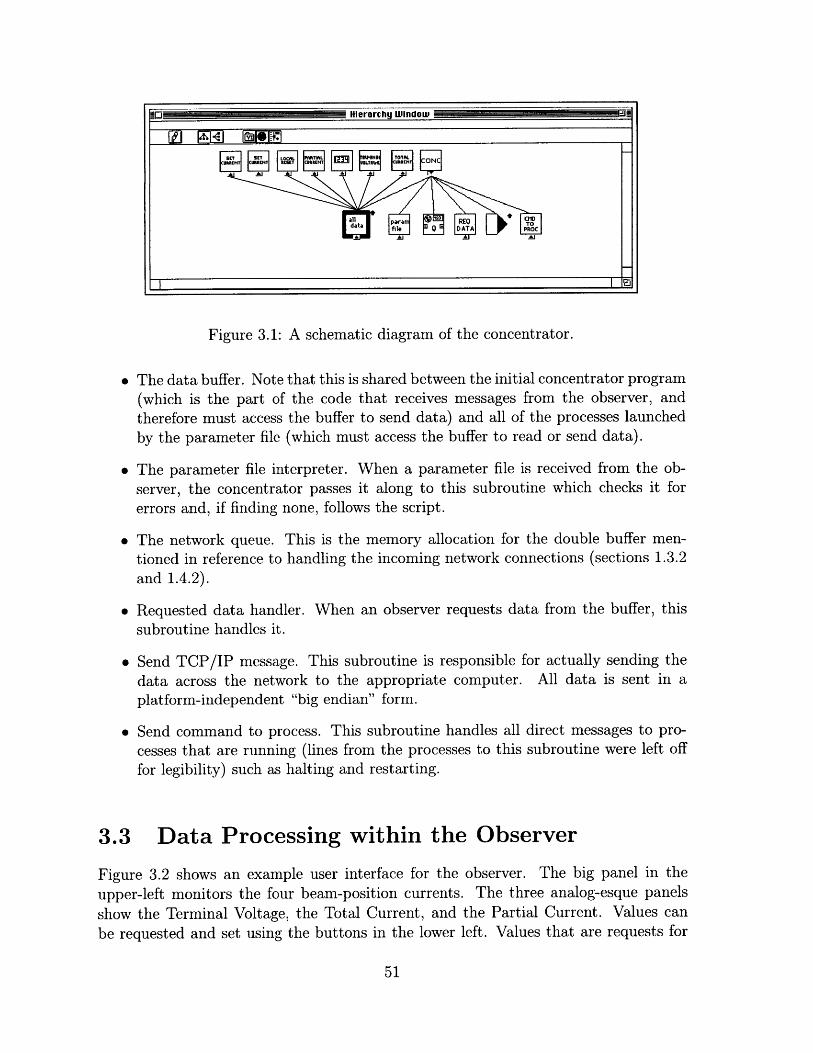
IQJ Hierarchy Window i!

Idat fl DATA PRO C

Figure 3.1: A schematic diagram of the concentrator.

* The data buffer. Note that this is shared between the initial concentrator program(which is the part of the code that receives messages from the observer, andtherefore must access the buffer to send data) and all of the processes launchedby the parameter file (which must access the buffer to read or send data).

* The parameter file interpreter. When a parameter file is received from the ob-server, the concentrator passes it along to this subroutine which checks it forerrors and, if finding none, follows the script.

* The network queue. This is the memory allocation for the double buffer men-tioned in reference to handling the incoming network connections (sections 1.3.2and 1.4.2).

* Requested data handler. When an observer requests data from the buffer, thissubroutine handles it.

* Send TCP/IP message. This subroutine is responsible for actually sending thedata across the network to the appropriate computer. All data is sent in aplatform-independent "big endian" form.

* Send command to process. This subroutine handles all direct messages to pro-cesses that are running (lines from the processes to this subroutine were left offfor legibility) such as halting and restarting.

3.3 Data Processing within the Observer

Figure 3.2 shows an example user interface for the observer. The big panel in theupper-left monitors the four beam-position currents. The three analog-esque panelsshow the Terminal Voltage, the Total Current, and the Partial Current. Values canbe requested and set using the buttons in the lower left. Values that are requests for

. .Observeruit

2 2 000 KigO~ f&7

Wo

-01 -02 -01 -0200 -0t 00 -T

::R -0 -01 -02

o o 3t0. ajo00 0300 -03

doooloi uofnl

jSu. of Chams -4m.1 currnt -1Ilil~

;Termnaul Volt Hat

concentrator address

lPatull Cu-rca(

IDoeCalculation OFF

Pulal Cu-rent do

10000 ~I te .. to... mantintaneoua doM

iSimulated Feedbac OFF

O new Terminal ol ultiply by gi

o-ui- t-e-u- -utt t2-t--s--( Iicute urro en Yj

L _ = ____jt

Total Cu-rei-50 -t00 -tOO

...00 -200

2000 0

-50 -50 -1 0

00 -_20 0

000

Deviation Calculations requires both

scan h 1-4 and sum of channels 1-4to be runnin,

ocot oo O F

ISum

Figure 3.2: The user interface of an observer.

data can be requested in two ways: by clicking the left button the value is requestedfor immediate delivery, by clicking the right button the value is sent when new datais available (event-driven mode). The parameter file can selected, edited and thendownloaded by clicking a button in the lower left as well. The remaining three groupsof buttons show "higher-level" calculations. The dose and instantaneous dose can becalculated by turning the appropriate box on. The dose calculation can be based oneither Partial Current or Total Current by means of a toggle switch. The simulatedfeedback box, when turned on, sets a current as a scaled value of the Terminal Voltagewhenever the Terminal Voltage value arrives at the observer (regardless of the meansby which it was requested). The percent deviation calculation, when selected, actuallyuses two values, which could (but don't) come from different concentrators. It looks tosee if the one of the beam-position currents is a certain percentage higher or lower thanthe average of the four, and sets a flag if it has. The individual currents is one value,and the sum of those four is another value, both required by this calculation. Whilethe example is trivial, as the sum could certainly be derived from the four individuals itrepresents the possibility of more meaningful, complex calculations based on multiplevalues.

Some examples of other possible complex computations for the observer follow.

U ~ i~;i~,,,,,..,,., i,, ;,~---- --- -- ----- -- -- -- -

I iti JM r4M-1jj 12pt Palatimo -li1M "-I1Z vl

* A running average, with possible weights.

* Integration or other methods of filtering values.

* Complex chart displays

* FFTs or other spectrum analyses.

54

Chapter 4

Performance Results

Included in this chapter are some charts showing some timing constraints of a workingconcentrator/observer system.

4.1 Timing the Buffer

The first figure, figure 4.1, shows a plot of access times in the buffer. This was doneoutside of the context of the concentrator or observer, it is merely a test of the comput-ers' ability to sort data. This test was setup as follows. N datapoints were placed intothe buffer (horizontal axis of the plot) as a certain value, all with different timestamps.The buffer was then asked to return all the datapoints since time zero in "peek-since"mode (defined in section 1.4.2), which will have the effect of returning all the data-points in the buffer for that value. The time it took to complete this request is shownon the vertical axis, in milliseconds. There are a couple of things to note about thisexperiment. First, it would be much more efficient to use "peek-all" mode, since weknow we are requesting all the data, but this test was designed as a worst case scenario.Second, the code for the buffer is not necessarily optimized in "peek-since" mode. Thecode assumes that the datapoints can be in the buffer for that value in any order,which is the only safe assumption. This is not optimal, however, if we know that thevalues will enter the buffer sequentially. In this case, the code could be modified toonly look for the first value whose timestamp comes after the requested time and thensend the remaining values. This would greatly increase the performance of the buffer,but at the cost of true generality in the system. Regardless, as expected the accesstime increases with the complexity of the request. The code is written to take time oforder N to service the request, and in the long run it does seem to be linear. The twocurves on the plot represent the results from two different computers, as described inthe legend.

Buffer Access Times

Figure 4.1: Access times for multiple reads from the buffer.

4.2 Calculating the Network Latency

Figure 4.2 exhibits a histogram of the latency in the network. In this experiment, thetime was recorded just after sending a request for one value ("peek-one") from thebuffer on a remote concentrator, and recorded again after the concentrator replied.The difference in these two times was recorded and was binned into a histogram. Notethat while most values are clustered, there are occasional requests that take a muchlonger time to return. This can be explained: the concentrator in question was runningfour processes in tandem, to simulate a busy system, during this test. If one of theseprocesses is writing to the buffer when the request to see data is received from theobserver, the request cannot be fulfilled until the buffer is no longer in use, therebystalling the system temporarily and increasing the latency time.

4.3 Exploring the Keithley

Figures 4.3 and 4.4 show the results of an experiment verifying the properties of theKeithley eight channel scanner that is used to measure the terminal voltage, partialcurrent, total current, and the four beam-position currents. The scanner has two res-

14000

12000

10000

8000

S 6000

4000

2000

0200 400 600 800 1000 1200 1400

number of datapoints

-- Power Mac 7200 - Pentium Pro 200

Network Delay

Figure 4.2: The latency in the network.

olutions with which it can operate: 4.5 decimal accuracy and 5.5 decimal accuracy.Furthermore, it has the option to filter the data while scanning, or it can just reportvalues without filtering. The four combinations of the above modes were tested forspeed. In both of these charts, the horizontal axis represents the number of pointsbuffered into the Keithley's memory before sent over the GPIB, by means of the pro-cess, and into the data buffer. The vertical axis is the time, in milliseconds, that theentire operation took. Figure 4.3 has the scanner reading one channel per instruction,as the process that manages the measuring of the terminal voltage would require; andfigure 4.4 has the scanner configured to read four channels in one shot, as the processthat monitors the four beam-position currents would need. The most apparent conclu-sion to draw from this figure is that if speed is a requirement, it is quite a detrimentto use both internal filtering and 5.5 digit resolution mode.

35

30

25

J 20

E 15

0I I, $ IIim I u 4 ; m u5m

miliseconds

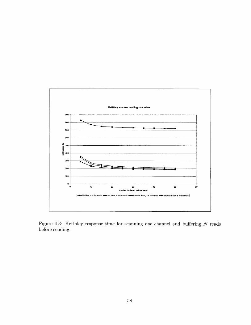
Keithley scanner reading one value.

900 ------

800

700

600

V500

400

300

200

100

0

0 10 20 30 40 50 60

number buffered before send

-- No filter, 4 5 decimals -- No filter, 5 5 decimals -- Internal Filter, 4 5 decimals -- Internal Filter, 5 5 decimals

Figure 4.3: Keithley response time for scanning one channel and buffering N readsbefore sending.

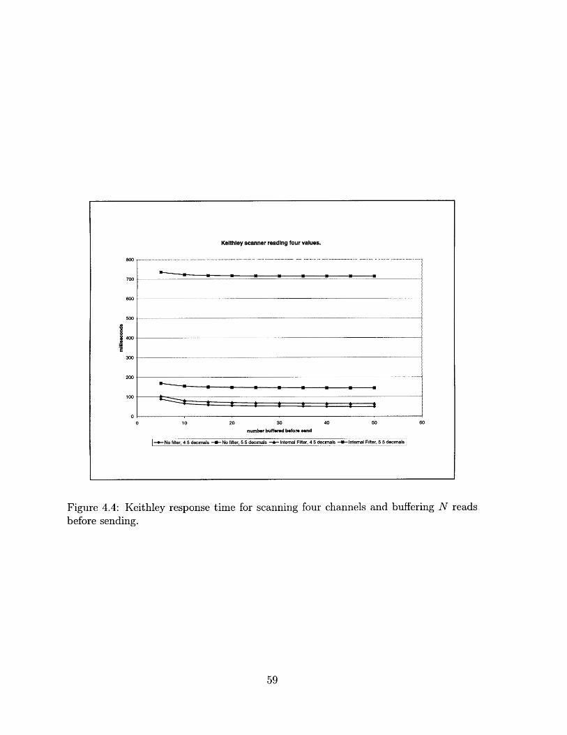
Keithley scanner reading four values.

800 -

700

600

500

I- 400

300

200

100

0 10 20 30 40 50 60

number buffered before send

I--*-No filter, 4 5 decimals --- No filter, 5 5 decimals -- Intemal Filter, 4 5 decimals -- Internal Filter, 5 5 decimals

Figure 4.4: Keithley response time for scanning four channels and buffering N readsbefore sending.

60

Chapter 5

Conclusion

This thesis has developed and followed into application a distributed method for ap-proaching digital control and monitoring. As the "Digital Age" continues there willbe more powerful computers available at trivial prices, and with them the expectationthat difficult tasks will be split among multiple computing resources. Gone are thedays of the mainframe where all applications must be run on one machine, locally.

The natural division between the concentrator and the observer makes this a veryintuitive scheme for devising a distributed monitoring and control system, one that istruly asynchronous and purely event-driven. Certainly, while the Van de Graaff controlsystem displays all the qualities of a concentrator/observer system, the system neednot be as simple or as focused. One can envision a large manufacturing plant with allof its controls and displays as concentrators and observers. While still being usableenough for any skilled operator to run, the system could include communication be-tween machines that have traditionally remained isolated, and use an observer-basedexpert-system to increase throughput. Or, leaving industrial controls altogether, onecan easily see how a home or business could profit from being able to externally monitorthe hot water and electricity usage all at one display, and use an appropriate controlalgorithm to prepare accurately prepare for high traffic times (when a lot of hot wateror electricity is being used) and to shut down in low traffic times. There are as manyapplications as there are traditional control systems waiting to be replaced by a modernsystem. This system's flexibility and expandability make it an ideal choice for control-ling large systems, particularly those complex enough to require many computers toperform all of the necessary calculations.

62

Appendix A

Example source code

Included for completeness are screenshots that exemplify the sourcecode of the con-centrator and the observer. Due to LabVIEW's graphical programming structure, itis impractical to include a complete transcript of the code here, the following figuresare simply examples. This may enlighten the reader slightly to the deuble-bufferednetwork connection scheme that both the concentrator and the observer uses. If thereader is unfamiliar with the LabVIEW programming language, he is encouraged toexamine manuals at the National Instruments web page, http://www.natinst. com.

Figure A.1 shows one state of the block diagram for the observer, and figure A.2does the same for the concentrator.

Fast Grab Conrcton

Figure A.1: The block diagram for the observer.

L Its asttabatue

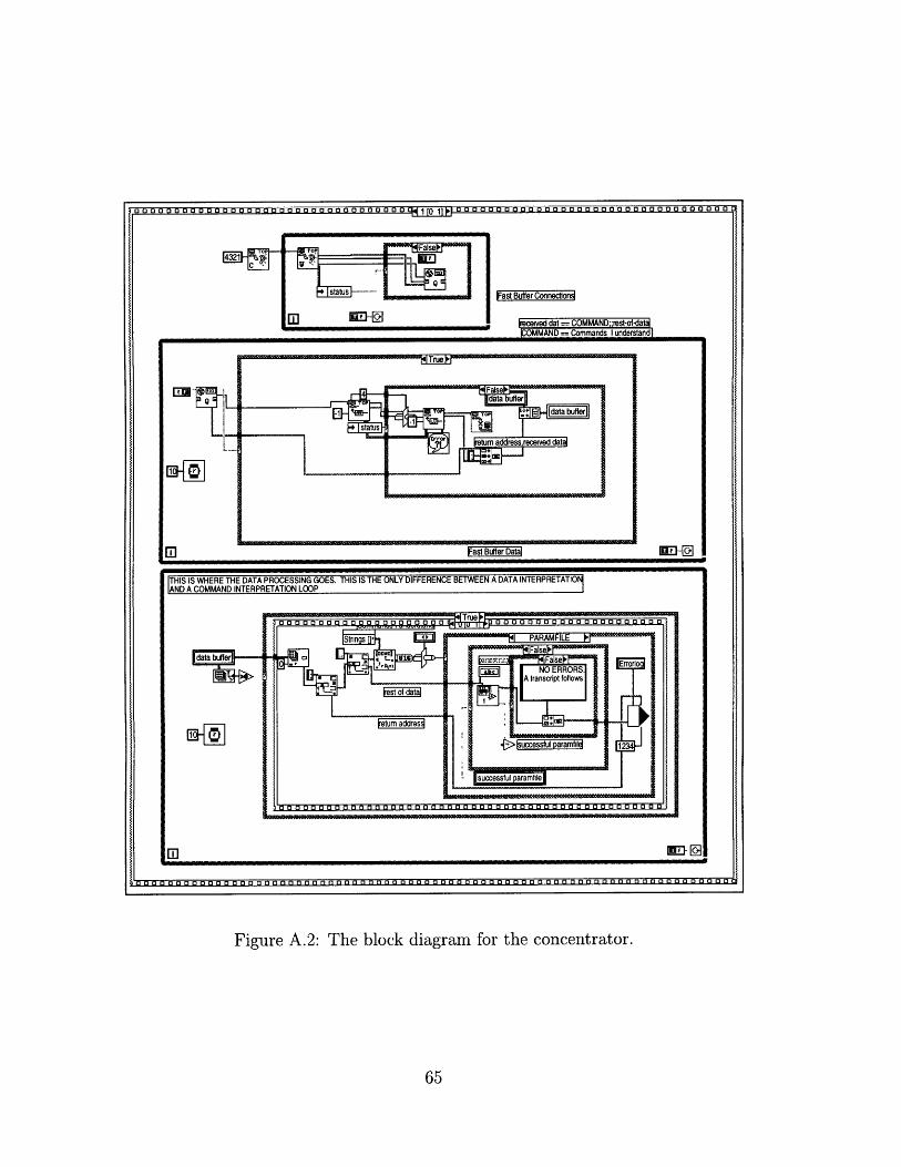
0 0 0 0 0 0 0 0 0 0 0 0 0 0 0 00 0 ~~g~oooo1ffioooooooooooooo~

Fast Buffer Connection

eceed dat == COMMAND;;rest-of-dataICOMMAND= Commands I understandl

Figure A.2: The block diagram for the concentrator.

THIS IS WHERE THE DATA PROCESSING GOES. THIS IS THE ONLY DIFFERENCE BETWEEN A DATA INTERPRETATIOAND A COMMAND INTERPRETATION LOOP

0o oIoooIo

00000000000003000000000000000000300 00Q 13 13 0tLLL0 000000000000000000000

66

Bibliography

[1] Astrom, Wittenmark, Computer Controlled Systems

[2] R. Bauman, T. Diaz, et. al, The Control of the Vivitron, Presented at the SNEAPConference (Jiilich), 1997

[3] J. G. Trump, K. A. Wright, A. M. Clarke Distribution of Ionization in Materi-als Irradiated by Two and Three Million-Volt Cathode Rays, Journal of AppliedPhysics, Volume 21, No. 3, pp. 345-348, 1950

[4] Bygrave, Treado, and Lambert. Accelerator Nuclear Physics - Fundamental Ex-

periments with a Van de Graaff Accelerator, High Voltage Engineering Corpora-tion, 1970

[5] C. M. Cooke, Dialectric Diagnosis and Expert Systems, ISH, 1995

[6] P. Katz, Digital Control Using Microprocessors, Prentice-Hall International, 1981

[7] A. S. Tanenbaum, Modern Operating Systems, Prentice-Hall Incorporated, 1992