evaluation of two statistical downscaling models for daily precipitation over an arid basin in china

INTERNATIONAL JOURNAL OF CLIMATOLOGYInt. J. Climatol. 31: 2006–2020 (2011)Published online 18 January 2011 in Wiley Online Library(wileyonlinelibrary.com) DOI: 10.1002/joc.2211

Evaluation of two statistical downscaling models for dailyprecipitation over an arid basin in China

Zhaofei Liu,a,b Zongxue Xu,a,c* Stephen P. Charles,d Guobin Fub,d and Liu Liua

a Key Laboratory of Water and Sediment Sciences, Ministry of Education, College of Water Sciences, Beijing Normal University,Beijing 100875, China

b Institute of Geographic Sciences and Natural Resources Research, Chinese Academy of Sciences, Beijing 100101, Chinac Xinjiang Institute of Ecology and Geography, Chinese Academy of Sciences, Urumqi 830011, China

d CSIRO Land and Water, Private Bag 5, Wembley, WA 6913, Australia

ABSTRACT: Two statistical downscaling (SD) models, the nonhomogeneous hidden Markov model (NHMM) and thestatistical down-scaling model (SDSM), which have been widely applied and proved skillful in terms of downscalingprecipitation, were evaluated based on observed daily precipitation over the Tarim River basin, an arid basin located inChina. The evaluated metrics included residual functions, correlation analyses, probability density functions (PDFs) anddistributions. Overall, both models exhibited stability with little model performance difference between the calibrationand validation periods. There was little difference for model performance on dry-spell length (dsl) and wet-spell length(wsl) between NHMM and SDSM. NHMM showed skill in simulating wet-day precipitation amount (wpa), whilst SDSMperformed relatively poorly on extreme values of wpa, especially for dry stations with annual precipitation lower than200 mm. Both NHMM and SDSM captured the spatial distribution characteristics of precipitation for most of the stations,as 11 months had an at-station correlation coefficient being greater than 0.9 and 0.8 for NHMM and SDSM in calibrationperiod. NHMM showed slightly better model performance than SDSM on simulating monthly precipitation, as the formerwas able to model precipitation well for all months, whereas the later was well only for certain months. SDSM was able tocapture the inter-site correlation characteristics of observed series, whilst the NHMM multi-site simulation over estimatedinter-site correlation. Both NHMM and SDSM had less skill downscaling annual series because of stochastic componentsin precipitation amounts modelling. Copyright 2011 Royal Meteorological Society

KEY WORDS hidden Markov model; NHMM; SDSM; model comparison; probability density function (PDF); extreme values

Received 1 January 2010; Revised 21 June 2010; Accepted 26 July 2010

1. Introduction

General circulation models or global climate models(GCMs), which are advanced mathematical models usedto simulate the present climate and project future cli-mate with forcing by greenhouse gases and aerosols,are the primary tool for capturing global climate sys-tem behaviour (Christensen et al., 2007). However, thespatial resolutions of GCMs are usually quite coarse (hun-dred kilometres) because of their significant complex-ity and the need to provide multi-century integrations.This results in the loss of regional and local details ofthe climate that are influenced by spatial heterogeneitiesmissing from these models. Therefore, GCM simulationsof local climate on spatial scales smaller than grid cellsare often poor, especially when the area has a complextopography (Schubert, 1998; McAvaney et al., 2001).Consequently, large-scale GCM scenarios should not beused directly for impact studies (Schubert and Sellers,

* Correspondence to: Zongxue Xu, Key Laboratory of Water andSediment Sciences, Ministry of Education, College of Water Sciences,Beijing Normal University, Beijing 100875, China.E-mail: [email protected]

1997), and generating information below the grid scale ofGCMs, which is referred to as downscaling, is needed inassessments for impact of climate change studies. Thereare two main approaches for downscaling: dynamical andstatistical (Christensen et al., 2007; Fowler et al., 2007).Fowler et al. (2007) reviewed downscaling techniquesand concluded that dynamical downscaling methods pro-vide little advantage over statistical techniques, at leastfor present day climates. Given the advantages of beingcomputationally inexpensive, able to access finer scalesthan dynamical methods and relatively easily applied todifferent GCMs, parameters and regions (Cubasch et al.,1996; Timbal et al., 2003; Wilby et al., 2004; Woodet al., 2004), statistical downscaling (SD) methods wereused in this study.

SD methods use empirical statistical techniques toestablish relationships between observed large-scale andregional/local climate (predictors and predictands) for abaseline period (Karl et al., 1990; Busuioc et al., 2001;Christensen et al., 2007). These relationships are thenapplied to downscale future climate scenarios using GCMoutput predictors. SD methods can be basically classified

Copyright 2011 Royal Meteorological Society

EVALUATION OF TWO STATISTICAL DOWNSCALING MODELS 2007

into three types (Wilby et al., 2004): regression mod-els (transfer functions), weather generators and weatherclassification. Regression models use linear or nonlinearmethods to represent relationships between predictandsand the large scale atmospheric forcing. Weather gener-ators, both unconditional (i.e. stationary) or conditional(i.e. using predictors), replicate the statistical attributes ofa local climate variable (such as the mean and variance)but not observed sequences of events (Wilks and Wilby,1999). Weather classification methods group days intofinite number of discrete weather types or ‘states’ accord-ing to their synoptic similarity. In general, SD methodswhich combine these techniques are often most effective(Christensen et al., 2007).

The statistical down-scaling model (SDSM) incorpo-rates both deterministic transfer functions and stochas-tic components (Wilby and Wigley, 1997; Wilby et al.,2002). SDSM has been widely applied in SD stud-ies for both climate variables and air quality variables(Diaz-Nieto and Wilby, 2005; Dibike and Coulibaly,2005; Khan et al., 2006; Wetterhall et al., 2006; Gachonand Dibike, 2007; Prudhomme and Davies, 2009; Wise,2009; and others), and has been recommended by theCanadian Climate Impacts and Scenarios (CCIS) project(http://www.cics.uvic.ca).

The nonhomogeneous hidden Markov model(NHMM), originally developed by Hughes and Guttorp(1994), simulates multi-site patterns of daily precipitationconditioned on a finite number of ‘hidden’ weather states.Therefore, the NHMM has weather classification andstochastic components. The NHMM has also had manysuccessful applications of downscaling daily precipitation(Bates et al., 1998; Charles et al., 1999; Hughes et al.,1999; Robertson et al., 2004). These studies have docu-mented that the NHMM is a promising method to repro-duce both daily precipitation occurrence and amount.

Comparisons between the SDSM and other down-scaling methods have shown that the SDSM performedwell in reproducing observed climate variability (Dibikeand Coulibaly, 2005; Diaz-Nieto and Wilby, 2005; Khanet al., 2006; Wetterhall et al., 2006; Gachon and Dibike,2007; Prudhomme and Davies, 2009). For example,Khan et al. (2006) compared three downscaling methods,SDSM, Long Ashton Research Station Weather Genera-tor (LARS-WG) model and an artificial neural network(ANN) for downscaling daily precipitation and maximumand minimum temperatures in a watershed of Canada andfound SDSM performed the best. Similar results werealso reported by Dibike and Coulibaly (2005). Althoughboth SDSM and LARS-WG were able to reproduce meandaily precipitation reasonable well, SDSM performed bet-ter in simulating variability of precipitation, and betterthan the perturbation method in the Thames Valley, UK(Diaz-Nieto and Wilby, 2005). Wetterhall et al. (2006)evaluated four SD methods for daily precipitation in threecatchments located in southern, eastern and central Chinaand northern Europe, and showed that SDSM performedbest.

The NHMM, although widely used in SD studies,has not been compared with other downscaling meth-ods as much as SDSM. Timbal et al. (2008) evalu-ated the NHMM and an analog approach for downscal-ing precipitation in southwest Western Australia. TheNHMM showed better model performance than the ana-log approach. Chiew et al. (2010) also compared severaldownscaling techniques and found that the NHMM to beone of the better performers. Therefore, the main aimof this study was to evaluate and compare these twowidely used models, SDSM and NHMM, for downscal-ing observed daily precipitation over the Tarim Riverbasin (TRB), an arid basin located in China (Xu et al.2010).

2. Methodology and datasets

2.1. Choice of predictors and predictor domains

Choice of predictor variables should be given highattention in applying SD (Wilby et al., 2004). Circulation-related predictors are usually selected as candidate pre-dictors, because observations (i.e. various reanalysisproducts) with relatively long series are available andGCMs simulate these with some skill (Cavazos andHewitson, 2005). However, it is increasingly acknowl-edged that circulation variables alone are not sufficient, asthey usually fail to capture key precipitation mechanismsbased on thermodynamics and moisture content. Thushumidity has increasingly been used to downscale precip-itation (e.g. Karl et al., 1990; Wilby and Wigley, 1997;Murphy, 1999), especially as it may be an important pre-dictor under a changed climate. It is suggested that theoptimal predictors must be strongly correlated with thepredictand, be physically sensible and capture multiyearvariability (Wilby and Wigley, 2000; Wilby et al., 2004;Gachon and Dibike, 2007). In this study, 20 NationalCenters for Environmental Prediction (NCEP) reanaly-sis (Kalnay et al., 1996) large-scale variables (Table I),which have potential physical relationships with pre-cipitation, were selected as candidate predictors. Thesepredictors include not only circulation variables (i.e.geopotential and wind component) but also temperature,radiation and moisture variables (specific humidity).

To avoid overfitting, it is well known that selectedpredictors should not be highly correlated, which wasconfirmed in this study as the model performance gen-erally improved when different types of variables wereincluded. If we only focused on explained variance ofprecipitation, then the same type variables (e.g. spe-cific humidity at several levels: shum400, shum500 andshum600) with high inter-correlations were more likelyto be selected. Therefore, both explained variance andpartial correlation analysis were used for choice of pre-dictors in this study to avoid this problem. Explainedvariance described the correlations between precipita-tion and the candidate predictors, while partial correla-tion analysis accounted for the correlations between thecandidate predictors themselves.

Copyright 2011 Royal Meteorological Society Int. J. Climatol. 31: 2006–2020 (2011)

2008 Z. LIU et al.

Table I. NCEP/NCAR candidate predictors.

ID Full name Classification

Air Air temperature Pressure levelvariables (three levels400 hPa, 500 hPa and600 hPa)

Hgt Geopotential heightShum Specific humidityuwnd East-west wind

velocityvwnd North-south wind

velocitySlp Air pressure at sea

levelSurface variables

Lhtfl Latent heat net flux atsurface

Shtfl Sensible heat net fluxat surface

nlwrs Net longwaveradiation flux atsurface

nswrs Net shortwaveradiation flux atsurface

NCEP, National Centers for Environmental Prediction; NCAR, NationalCenter for Atmospheric Research.

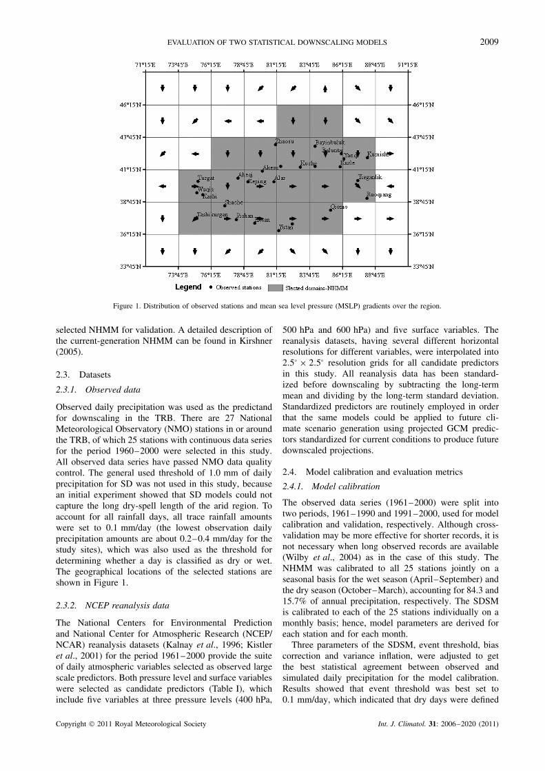
The choice of predictor domain, which is generallylittle reported, has also been found to be a critical fac-tor affecting downscaled results (Goodess and Palutikof,1998; Benestad et al., 2001; Tomozeiu et al., 2007), espe-cially for downscaling precipitation (Wilby and Wigley,2000), because single-grid predictors are not necessar-ily related to an underlying location (Brinkmann, 2002).Therefore, multi-grid predictor domains were selected foreach observed station in the application of SDSM. Poten-tial grids include the grid nearest to the observed stationand the eight grids surrounding it. The predictor domainswere selected from these candidate potential grids basedon mean sea level pressure gradients. For each station, thecentre grid in which a station was located and its neigh-bour grids which have a mean sea level pressure gradient(Figure 1) towards this centre grid were selected as thegrid domain for the station in SDSM. The boundary of theTarim River catchment was used for the NHMM domainas shown by grey grids in Figure 1.

2.2. Model descriptions

2.2.1. Statistical down-scaling model

As mentioned above, SDSM uses a hybrid stochasticweather generator and multi-linear regression method tosimulate local precipitation at each station conditionalon regional circulation and atmospheric moisture pre-dictors (Harpham and Wilby, 2005). The multi-linearregression derives a statistical relationship between pre-dictors and precipitation (Wetterhall et al., 2006). Pre-cipitation is then modelled by the stochastic weather

generator to replicate the observed variability, becausethe chaotic nature of local weather conditions cannot befully explained by the variations in predictor variablesalone (Prudhomme and Davies, 2009). Therefore, SDSMenables generation of multiple simulations with slightlydifferent time series attributes, but the same overall sta-tistical properties. The detailed technical information ofSDSM can be found in Wilby et al. (2002).

Generally, the application of SDSM contains five steps(Wilby et al., 2000, 2002, 2006): (1) selection of pre-dictors; (2) model parameter calibration; (3) simulation;(4) model validation and (5) generation of future seriesof the predictand. As the purpose of this study is toevaluate the performance of two downscaling methodsfor downscaling observed precipitation, Step 5 was notincluded. Model calibration involves optimizing multi-ple linear regression equations for daily precipitation asa function of the selected large-scale atmospheric vari-able NCEP reanalysis predictors. Then, daily precipita-tion was simulated by the weather generator in the model,driven by NCEP reanalysis predictors. Evaluation of themodel is based on comparison between the simulated andobserved daily precipitation series.

2.2.2. Nonhomogeneous hidden Markov model

The NHMM defines stochastic conditional relationshipsbetween multi-site daily precipitation patterns and a dis-crete set of weather states, which are hidden statesbecause they are not directly observable (Charles et al.,1999; Robertson et al., 2004; Greene et al., 2008). Theformulation of the NHMM reproduces the spatial struc-ture of multi-site patterns of precipitation. The transi-tion probabilities between the hidden states, conditionalon the set of predictors, are defined by a first-orderMarkov chain (Robertson et al., 2004). Daily precipita-tion amounts for each station are simulated based on thegamma distribution. By conditioning precipitation on hid-den states, rather than atmospheric circulation patterns,the NHMM captures much of the spatial and tempo-ral variability of daily multi-site precipitation records(Charles et al., 1999).

The application of the NHMM to a selected networkof precipitation stations consists of five steps (Robert-son et al., 2004; Greene et al., 2008): (1) selection ofnumber of hidden states; (2) selection of predictors;(3) calibration; (4) simulation and (5) model validation.The most appropriate number of hidden states is esti-mated based on maximum likelihood, as evaluated bythe Bayes information criterion (BIC) (Robertson et al.,2004). Once the number of hidden states has been esti-mated, the most likely daily sequence of hidden statescan be determined by the Viterbi algorithm (Forney,1978). Thus, although the weather states are statisticalconstructs of the model, they could be examined by clas-sifying each day into its most probable weather state andconstructing composite plots of the associated precipi-tation patterns and atmospheric predictor fields. Simu-lations of multi-site precipitation were generated by the



Figure 1. Distribution of observed stations and mean sea level pressure (MSLP) gradients over the region.

selected NHMM for validation. A detailed description ofthe current-generation NHMM can be found in Kirshner(2005).

2.3. Datasets

2.3.1. Observed data

Observed daily precipitation was used as the predictandfor downscaling in the TRB. There are 27 NationalMeteorological Observatory (NMO) stations in or aroundthe TRB, of which 25 stations with continuous data seriesfor the period 1960–2000 were selected in this study.All observed data series have passed NMO data qualitycontrol. The general used threshold of 1.0 mm of dailyprecipitation for SD was not used in this study, becausean initial experiment showed that SD models could notcapture the long dry-spell length of the arid region. Toaccount for all rainfall days, all trace rainfall amountswere set to 0.1 mm/day (the lowest observation dailyprecipitation amounts are about 0.2–0.4 mm/day for thestudy sites), which was also used as the threshold fordetermining whether a day is classified as dry or wet.The geographical locations of the selected stations areshown in Figure 1.

2.3.2. NCEP reanalysis data

The National Centers for Environmental Predictionand National Center for Atmospheric Research (NCEP/NCAR) reanalysis datasets (Kalnay et al., 1996; Kistleret al., 2001) for the period 1961–2000 provide the suiteof daily atmospheric variables selected as observed largescale predictors. Both pressure level and surface variableswere selected as candidate predictors (Table I), whichinclude five variables at three pressure levels (400 hPa,

500 hPa and 600 hPa) and five surface variables. Thereanalysis datasets, having several different horizontalresolutions for different variables, were interpolated into2.5° × 2.5° resolution grids for all candidate predictorsin this study. All reanalysis data has been standard-ized before downscaling by subtracting the long-termmean and dividing by the long-term standard deviation.Standardized predictors are routinely employed in orderthat the same models could be applied to future cli-mate scenario generation using projected GCM predic-tors standardized for current conditions to produce futuredownscaled projections.

2.4. Model calibration and evaluation metrics

2.4.1. Model calibration

The observed data series (1961–2000) were split intotwo periods, 1961–1990 and 1991–2000, used for modelcalibration and validation, respectively. Although cross-validation may be more effective for shorter records, it isnot necessary when long observed records are available(Wilby et al., 2004) as in the case of this study. TheNHMM was calibrated to all 25 stations jointly on aseasonal basis for the wet season (April–September) andthe dry season (October–March), accounting for 84.3 and15.7% of annual precipitation, respectively. The SDSMis calibrated to each of the 25 stations individually on amonthly basis; hence, model parameters are derived foreach station and for each month.

Three parameters of the SDSM, event threshold, biascorrection and variance inflation, were adjusted to getthe best statistical agreement between observed andsimulated daily precipitation for the model calibration.Results showed that event threshold was best set to0.1 mm/day, which indicated that dry days were defined


2010 Z. LIU et al.

Figure 2. Bayes information criterion (BIC) with differing numbers of hidden states (a) for the wet season model; (b) for the dry season model.This figure is available in colour online at wileyonlinelibrary.com/journal/joc

when daily precipitation was less than 0.1 mm/day,while wet days were defined when it was greater than0.1 mm/day. The relative errors of long-term annualprecipitation were used to calibrate bias correction andvariance inflation.

The choice of the appropriate number of hidden statesin the NHMM was based on BIC indices for both wet anddry season models, respectively, for the calibration period(1961–1990) in which observed station precipitation dataand selected NCEP predictor data were used. Resultsshowed that the BIC reached their minimum values whenhidden state numbers were six and three for the wetand dry seasons, respectively (Figure 2). These wereselected as the appropriate number of hidden states forthe NHMM.

Several event thresholds for wet and dry days werecalibrated and a similar result as that of SDSM wasobtained: the best model performance was achieved withan event threshold of 0.1 mm/day.

2.4.2. Evaluation metrics

Several objective functions were selected for modelevaluation in this study. All objective functions wereevaluated both for the model calibration (1961–1990)and validation (1991–2000). The predictor sets and theirdomains fixed in the calibration period were used in thevalidation period.

Firstly, residual functions were used to compare thedifferences of statistical properties between observedand simulated precipitation series. The model bias wasevaluated by the relative error (RE) of long-term annualprecipitation at each individual station. Extreme events,which are of interest in climate impact assessments,were evaluated by the 50th, 90th and 99th percentiles ofthe wet-day precipitation amount (wpa), wet-spell length(wsl) and dry-spell length (dsl).

The correlation coefficient was used to assess thewithin-year (i.e. intra-annual) cycle and at-station distri-bution of precipitation. For intra-annual cycle assessment,the correlation coefficient was calculated with observedand simulated long-term monthly mean values for thesample size of 12 (the number of months). For at-stationdistribution assessment, the correlation coefficient wascomputed with observed and simulated long-term meanvalues for each station. The sample size is 25, the numberof stations.

Two skill metrics, the Brier score (BS) and the skillscore (Sscore), based on probability density functions(PDFs), were used to measure how well each model cancapture the PDFs of wpa, wls and dsl distributions, andwere computed by:

BS = 1

n

n∑

i=1

(Pmi − Poi)2 (1)

Sscore =n∑

i=1

Minimum(Pmi, Poi) (2)

where Pmi and Poi are the modelled and observed ithprobability values of each bins and n is the number ofbins. The BS is a mean squared error measure used forprobability forecasts (Brier, 1950), and Sscore calculatesthe cumulative minimum value between observed andmodelled distributions for each binned value, therebymeasuring the overlap area between two PDFs (Perkinset al., 2007).

The quantile–quantile (Q–Q) plot (Gnanadesikan andWilk, 1968) is a graphical method for comparingtwo probability distributions by plotting their quantilesagainst each other. If the two distributions being com-pared are similar, the points in the Q–Q plot will approx-imately lie on the line y = x. If the distributions arelinearly related, the points in the Q–Q plot will approxi-mately lie on a line, but not necessarily on the line y = x.

3. Results

3.1. Predictor selection

Table II presents the predictors selected in SDSM andNHMM calibration. The shum400, vwnd500, shtfl, lhtfl,nlwrs, slp and air500 were selected as predictors forthe NHMM, based on explained variances and partialcorrelation analysis. These predictors are consistent withthe dynamic mechanism of precipitation in the TRB,which is mainly controlled by westerly water vapourtransport (Dai et al., 2007; Qian and Qin, 2008). Predictorsets were varied for each individual station for the SDSM.Overall, the selected predictor number for each stationwas between five and seven: shum and vwnd were themost selected predictors, shtfl, lhtfl, nlwrs, slp, uwnd andair followed, while other variables were rarely selected.



Table II. Explained variances of each predictor and SDSM and NHMM selected predictors.

Variables Explained variance Selectiona Variables Explained variance Selectiona

air400 0.316 – uwnd500 0.074 –air500 0.213 9b uwnd600 0.074 6air600 0.237 5 vwnd400 0.060 –hgt400 0.203 – vwnd500 0.052 17b

hgt500 0.182 – vwnd600 0.047 6hgt600 0.181 – slp 0.039 18b

shum400 0.181 9b lhtfl 0.037 20b

shum500 0.180 5 shtfl 0.028 21b

shum600 0.150 11 nlwrs 0.027 19b

uwnd400 0.095 4 nswrs 0.023 5

SDSM, statistical down-scaling model; NHMM, nonhomogeneous hidden Markov model.a Number of stations selected as predictor by SDSM.b Indicates selected by NHMM.

Figure 3. Box plots of relative errors for monthly and annual precipitation across all stations: the horizontal lines represent the median values;the Interquartile Range (IQR, i.e. 25th–75th quantiles) is represented by boxes; the whiskers indicate the lowest value within the lower limit ofQ1 − 1.5(Q3 − Q1) and the highest data value within the upper limit of Q3 + 1.5(Q3 − Q1), respectively; values beyond the whiskers are

outliers (asterisks).

3.2. Comparison between two downscaling models

3.2.1. Residual functions

Relative errors of annual precipitation for SDSM andNHMM at each station are shown in Figure 3. In general,both SDSM and NHMM performed well in simulatingmean annual precipitation with relative errors at moststations being less than 20%. Overall, NHMM showedslightly better model performance for the mean annualprecipitation than SDSM. Models biases of long-termmean monthly precipitation for the two models are alsoshown in Figure 3. Median relative errors of NHMMfor all stations were lower than 20% in most of themonths except for April and December. Median relativeerrors of SDSM were lower than 20% only from Juneto September, in which precipitation takes more than60% of annual precipitation. SDSM shows higher relativeerrors in other months, especially for dry season monthswith median values for all stations larger than 50%. Ingeneral, relative errors of monthly precipitation simulatedby NHMM were lower than those simulated by SDSM.

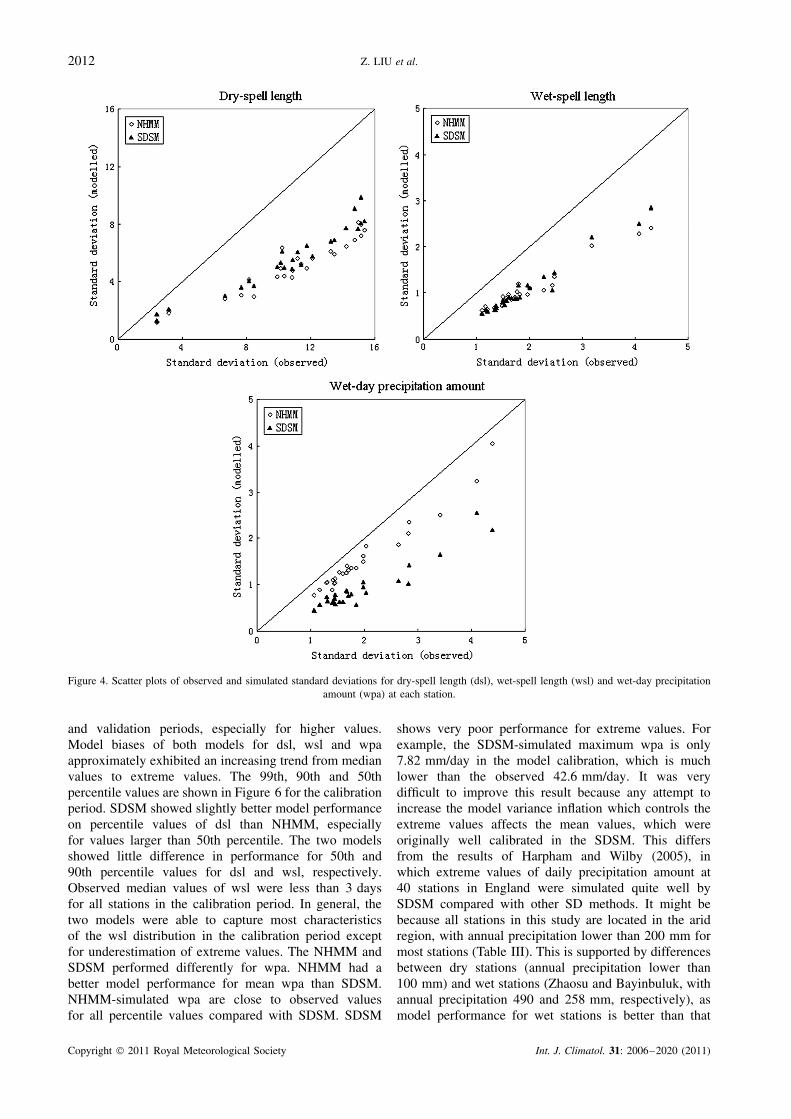
Figure 4 compares the standard deviations of observedand downscaled dsl, wsl and wpa for all stations. Bothmodels consistently under-represent standard deviationsfor all statistics. There is a noticeable difference in model

performance between relatively dry and wet stations (seeTable III to distinguish between lower and higher annualprecipitation stations). For dsl and wpa, model biases ofstandard deviation at relatively wet stations (most notablyat Turgat and Bayinbuluk) were lower than that at rela-tively dry stations. Conversely, the largest biases for wslwere at relatively wet stations. Both NHMM and SDSMshow better performance at wet stations for wpa and dsl,while showing better performance at dry stations for wsl.The mean value of standard deviation biases betweenobserved and downscaled dsl for all stations is 0.49 forNHMM, compared with 0.41 for SDSM. Similarly, bothmodels show mean biases with 0.39 for wsl. There waslittle difference between NHMM and SDSM for stan-dard deviation of wsl, while SDSM showed slightly bettermodel performance than NHMM for standard deviationof dsl. Large differences in simulating standard deviationof wpa are seen at all stations, with mean biases 0.22 forNHMM, compared with 0.53 for SDSM. This was causedby the underestimation of extreme wet-day precipitationamounts, as seen in Figure 5 (The model performance foreach station can be found in Table III).

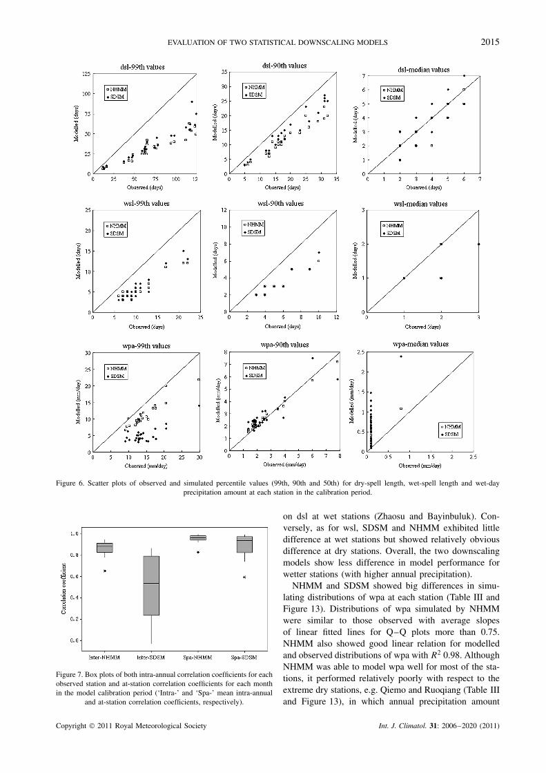
Both NHMM and SDSM underestimated the selectedpercentile values of dsl, wsl and wpa in the calibration


2012 Z. LIU et al.

Figure 4. Scatter plots of observed and simulated standard deviations for dry-spell length (dsl), wet-spell length (wsl) and wet-day precipitationamount (wpa) at each station.

and validation periods, especially for higher values.Model biases of both models for dsl, wsl and wpaapproximately exhibited an increasing trend from medianvalues to extreme values. The 99th, 90th and 50thpercentile values are shown in Figure 6 for the calibrationperiod. SDSM showed slightly better model performanceon percentile values of dsl than NHMM, especiallyfor values larger than 50th percentile. The two modelsshowed little difference in performance for 50th and90th percentile values for dsl and wsl, respectively.Observed median values of wsl were less than 3 daysfor all stations in the calibration period. In general, thetwo models were able to capture most characteristicsof the wsl distribution in the calibration period exceptfor underestimation of extreme values. The NHMM andSDSM performed differently for wpa. NHMM had abetter model performance for mean wpa than SDSM.NHMM-simulated wpa are close to observed valuesfor all percentile values compared with SDSM. SDSM

shows very poor performance for extreme values. Forexample, the SDSM-simulated maximum wpa is only7.82 mm/day in the model calibration, which is muchlower than the observed 42.6 mm/day. It was verydifficult to improve this result because any attempt toincrease the model variance inflation which controls theextreme values affects the mean values, which wereoriginally well calibrated in the SDSM. This differsfrom the results of Harpham and Wilby (2005), inwhich extreme values of daily precipitation amount at40 stations in England were simulated quite well bySDSM compared with other SD methods. It might bebecause all stations in this study are located in the aridregion, with annual precipitation lower than 200 mm formost stations (Table III). This is supported by differencesbetween dry stations (annual precipitation lower than100 mm) and wet stations (Zhaosu and Bayinbuluk, withannual precipitation 490 and 258 mm, respectively), asmodel performance for wet stations is better than that



Table III. Linear relation for Q–Q plot.

Stations dsl wsl wpa Annual precipitation (mm)

SDSM NHMM SDSM NHMM SDSM NHMM

k R2 k R2 k R2 k R2 k R2 k R2

Aheqi 0.43 0.96 0.38 0.98 0.57 0.97 0.49 0.97 0.23 0.54 0.82 0.99 188Akesu 0.51 0.97 0.43 0.97 0.41 0.93 0.46 0.95 0.17 0.50 0.71 0.99 69Alar 0.56 0.96 0.52 0.96 0.34 0.89 0.39 0.92 0.33 0.70 0.85 0.99 50Bluntai 0.78 0.97 0.78 0.98 0.73 0.93 0.65 0.94 0.32 0.63 0.73 0.99 191Baicheng 0.45 0.97 0.30 0.93 0.30 0.91 0.31 0.89 0.29 0.64 0.89 0.98 109Hotan 0.57 0.99 0.42 0.96 0.39 0.91 0.32 0.87 0.24 0.58 0.86 0.98 36Kashi 0.49 0.97 0.44 0.98 0.54 0.93 0.47 0.91 0.16 0.62 0.83 0.98 67Keping 0.64 0.99 0.43 0.98 0.54 0.96 0.51 0.96 0.24 0.50 0.82 1.00 87Kuche 0.50 0.95 0.41 0.95 0.45 0.92 0.50 0.93 0.24 0.56 0.68 0.99 69Kurle 0.58 0.98 0.52 0.98 0.40 0.92 0.42 0.88 0.18 0.48 0.95 0.99 57Kumishi 0.49 0.95 0.44 0.95 0.46 0.92 0.45 0.86 0.21 0.53 0.63 0.98 49Luntai 0.52 0.97 0.49 0.98 0.44 0.91 0.48 0.93 0.16 0.50 0.78 1.00 61Minfeng 0.70 0.98 0.44 0.98 0.41 0.85 0.41 0.86 0.16 0.45 0.65 0.98 37Pishan 0.54 0.99 0.43 0.98 0.41 0.89 0.34 0.85 0.17 0.49 0.70 0.99 49Qiemo 0.50 0.95 0.49 0.98 0.35 0.86 0.39 0.89 0.15 0.54 0.53 0.96 28Ruoqiang 0.55 0.95 0.58 0.96 0.29 0.81 0.42 0.86 0.16 0.61 0.38 0.91 28Tashikurgan 0.48 0.98 0.51 0.99 0.49 0.95 0.37 0.92 0.15 0.43 0.57 0.98 72Tieganlik 0.53 0.94 0.63 0.99 0.42 0.88 0.51 0.89 0.42 0.88 0.80 1.00 39Turgat 0.53 0.96 0.46 0.96 0.62 0.99 0.50 0.98 0.24 0.73 0.62 0.97 236Wuqa 0.47 0.98 0.43 0.98 0.61 0.95 0.41 0.95 0.16 0.52 0.77 0.99 165Yanqi 0.50 0.98 0.38 0.94 0.39 0.91 0.39 0.90 0.20 0.58 1.07 0.98 73Yutan 0.72 0.98 0.48 0.96 0.38 0.82 0.36 0.79 0.27 0.67 0.78 0.99 47Shache 0.51 0.98 0.50 0.99 0.47 0.92 0.35 0.90 0.13 0.43 0.76 1.00 49Bayinbuluk 0.73 0.97 0.43 0.96 0.76 0.93 0.54 0.99 0.32 0.69 0.92 0.99 258Zhaosu 0.67 0.98 0.55 0.98 0.81 0.97 0.65 0.98 0.31 0.68 0.94 1.00 490Average 0.56 0.97 0.47 0.97 0.48 0.91 0.44 0.91 0.22 0.58 0.76 0.98

dsl, dry-spell length; wsl, wet-spell length; wpa, wet-day precipitation amount; SDSM, statistical down-scaling model; NHMM, nonhomogeneoushidden Markov model.k is the slope of linear fitted line for the Q–Q plot, which is perfect for 1; R2 describes the degree of linear relation for observed and modeleddistributions, which is also perfect for 1.

for dry stations. Overall, NHMM simulates both wpadistribution shape and extreme values, whereas SDSMhas poor performance for extreme values, especially fordry stations with annual precipitation lower than 200 mm.

3.2.2. Correlation analysis of seasonal-cycle andat-station distributions

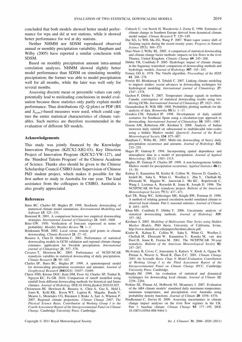
Results for correlation analysis of seasonal-cycle and at-station distribution are shown in Figure 7. In general,both models could capture well the at-station distributioncharacteristics of observed precipitation, as 11 monthshad an at-station correlation coefficient being larger than0.9 and 0.8, respectively, for NHMM and SDSM in thecalibration period. It could also be noted that NHMM per-formed a little better than SDSM on simulating at-stationdistribution characteristics for most stations. The medianat-station correlation coefficient was larger than 0.95 forthe NHMM model calibration period, and NHMM alsoperformed well for the validation period with median val-ues nearly to 0.9. Although not performing as well as theNHMM, SDSM was also able to capture at-station dis-tribution characteristics of precipitation, with a medianvalue of at-station correlation coefficient nearly to 0.9

for both calibration and validation periods. However, itshould be noted that the SDSM is calibrated to each sta-tion independently and so is not a spatial model, whereasthe NHMM calibrates to all station simultaneously andis fully spatial, so daily sequences would have the cor-rect spatial coherence for the NHMM but not for SDSM.NHMM-modelled intra-annual data series have high cor-relation coefficients for almost all observed stations in thecalibration period, with most station’s correlation coef-ficient larger than 0.8. Although SDSM could simulatelong-term annual mean precipitation well (Figure 3), itperformed relatively poorly for intra-annual cycle char-acteristics. In the calibration period, intra-annual cyclecorrelation coefficients were less than 0.5 for 11 stations,2 stations even with negative correlation coefficients.

In contrast to performance for intra-annual and at-station distribution, both NHMM and SDSM showedlittle ability in downscaling annual series inter-annualvariability with relatively lower correlation coefficientsfor annual series of monthly and annual precipitation(Figure 8). The stochastic nature of the simulation ofthe precipitation amounts in NHMM and SDSM, whichmeans that any downscaled precipitation series would not


2014 Z. LIU et al.

Figure 5. Distributions of modelled and observed average wet-day precipitation amount of all stations in the model calibration (the distributionswere fit based on the Gamma distribution).

be expected to exactly match observations, might explainpart of this. This is consistent with results of Harphamand Wilby (2005), in which annual series of precipitationamounts were downscaled by SDSM with least skill.

As mentioned above, the dynamic mechanism ofprecipitation generation in the basin is mainly controlledby westerly water vapour transport (Dai et al, 2007;Qian and Qin, 2008). However, the inter-site correlationcoefficients of the annual cycle series were less than0.8, with most of the values between 0.2 and 0.5(Figure 9). SDSM was able to capture this character ofinter-site correlation better than NHMM. The NHMMoverestimated inter-site correlation.

3.2.3. Skill scores based on PDFs

The results of two PDF-based skill scores Sscore and BSindicated that there is little difference between NHMMand SDSM performance simulating dsl and wsl, withboth models showing good skill with high stabilities(Figure 10). However, skills of the two models showa larger difference simulating wpa, with NHMM bettersimulated wpa than SDSM. Overall, NHMM shows verygood skill in modelling wpa, dsl and wsl, especiallyfor wpa with Sscore greater than 0.9 for both calibrationand validation periods. SDSM also shows good skillin modelling dsl and wsl with Sscore being greater than0.75 for all stations used in this study. However, SDSMdoes not show skill for wpa, potentially because of itspoor performance on extreme values. There was little

difference for model performance of NHMM and SDSMbetween the calibration and validation periods, whichcould also be found in other statistics (such as residualfunctions and correlation analyses) but not shown. Thisindicates that both models are stable in downscaling dailyprecipitation at all stations.

3.2.4. Q–Q plots

Linear relationships for Q–Q plots of observed and mod-elled dsl, wsl and wpa for SDSM and NHMM at allstations are presented in Table III. Although the twodownscaling models’ simulated distributions of dsl andwsl were not exactly the same as observed, with the aver-age slopes of linear fitted lines for the Q–Q plots about0.5, the distributions modelled by the two models showedoverall linear relationship with observed, with average R2

more than 0.9, especially for dsl with average R2 0.97.There was little difference in model performance for dis-tributions of dsl and wsl between SDSM and NHMM,with SDSM showing slightly better performance, espe-cially for dsl at relatively wet stations (Figure 11), e.g.Zhaosu, Bayinbuluk. Q–Q plots of dsl, wsl and wpa atsix typical stations, which represent different levels ofannual precipitation amounts (Table III), are also shownin Figures 11–13. These reveal that both models tendto underestimate dsl and wsl at all stations, especiallyfor higher values. The two models show little differencein performance on dsl at dry stations (Shache and Ruo-qiang), but have obviously different model performance



Figure 6. Scatter plots of observed and simulated percentile values (99th, 90th and 50th) for dry-spell length, wet-spell length and wet-dayprecipitation amount at each station in the calibration period.

Figure 7. Box plots of both intra-annual correlation coefficients for eachobserved station and at-station correlation coefficients for each monthin the model calibration period (‘Intra-’ and ‘Spa-’ mean intra-annual

and at-station correlation coefficients, respectively).

on dsl at wet stations (Zhaosu and Bayinbuluk). Con-versely, as for wsl, SDSM and NHMM exhibited littledifference at wet stations but showed relatively obviousdifference at dry stations. Overall, the two downscalingmodels show less difference in model performance forwetter stations (with higher annual precipitation).

NHMM and SDSM showed big differences in simu-lating distributions of wpa at each station (Table III andFigure 13). Distributions of wpa simulated by NHMMwere similar to those observed with average slopesof linear fitted lines for Q–Q plots more than 0.75.NHMM also showed good linear relation for modelledand observed distributions of wpa with R2 0.98. AlthoughNHMM was able to model wpa well for most of the sta-tions, it performed relatively poorly with respect to theextreme dry stations, e.g. Qiemo and Ruoqiang (Table IIIand Figure 13), in which annual precipitation amount


2016 Z. LIU et al.

Figure 8. Box plots of correlation coefficients between observed and modelled annual series of monthly and annual precipitation.

Figure 9. Inter-site correlation coefficient of daily precipitation amountfor all stations.

was only 28 mm (Table III). SDSM showed satisfactorymodel performance for linear relation of modelled andobserved distributions of wpa with R2 close to 0.6, butperformed poorly on similarities of distributions withslopes only up to 0.42. It showed a very poor perfor-mance on extreme values for all stations, including thesix typical stations shown in Figure 13.

4. Discussion and conclusion

This study evaluated two widely used SD models,NHMM and SDSM, based on their simulation of dailyprecipitation over the TRB, which is an arid region withannual precipitation lower than 200 mm for most stations(Table III). Results showed that there was little differ-ence for model performance on dsl and wsl betweenNHMM and SDSM, but NHMM exhibited better perfor-mance than SDSM for wpa. Both models exhibited skillsfor model stability with little model performance differ-ence between the calibration and validation periods. Morespecifically, the following conclusions are made.

The choice of predictors and predictor domains wasan important step in the application of SD techniquesbecause it has a great impact on the downscaling results.In this study, multiple grids, which were selected basedon mean sea level pressure gradients, were used as pre-dictor domains to capture more circulation conditionsrelated to local physical precipitation mechanisms. It wasfound that moisture and wind variables (shum and vwnd)had the strongest relationship with precipitation, whichwas consistent with the dynamic mechanisms of pre-cipitation in the TRB. Other candidate predictors suchas air temperature, mean sea level pressure and radi-ation variables, which had strong statistical relation-ships with precipitation, were also selected for down-scaling models because of their contribution to localprecipitation.

NHMM showed skill in simulating wpa, while SDSMperformed relatively poorly on extreme values of wpa,especially for dry stations with annual precipitation lowerthan 200 mm. This was different from the performance ofSDSM on wet stations in England (Harpham and Wilby,2005), in which extreme values of daily precipitationamount were well simulated by SDSM compared withother SD methods. It is concluded that SDSM tends tolose skill when simulating extreme precipitation amountat relatively dry stations located in arid regions.

Both NHMM and SDSM could capture the spatialdistribution characteristics of precipitation in the TRB,with the NHMM performing a little better. This may beattributed to the NHMM including spatial correlationsfor modelling multi-site precipitation, which is missingin SDSM as it models each individual station separately.This conclusion is consistent with results of Wetterhallet al. (2006), comparing SDSM with a fuzzy-rule-basedweather-pattern-classification method for simulating dailyprecipitation in three catchments of China, which con-cluded that the SDSM had the disadvantage of modellingeach station separately. As for the correlation betweendifferent stations, SDSM was able to capture the inter-sitecorrelation characters of observed series, while NHMMoverestimated the inter-site correlation.

There is difference in performance between relativelydry stations and wet stations for both models. It was



Figure 10. Interval plots of two skill scores for wet-spell length, dry-spell length and wet-day precipitation amount of each station in the modelcalibration and validation, (a) and (b) are for skill score (Sscore) in the calibration and validation, respectively; whereas (c) and (d) are the same

but for Brier score (BS). This figure is available in colour online at wileyonlinelibrary.com/journal/joc

Figure 11. Quantile–quantile plots for dry-spell length (dsl) at typical stations for the calibration period.


2018 Z. LIU et al.

Figure 12. Quantile–quantile plots for wet-spell length (wsl) at typical stations for the calibration period.

Figure 13. Quantile–quantile plots for wet-day precipitation amount (wpa) at typical stations for the calibration period.



concluded that both models showed better model perfor-mance for wpa and dsl at wet stations, while it showedbetter performance for wsl at dry stations.

Neither NHMM nor SDSM reproduced observedannual or monthly precipitation variability. Harpham andWilby (2005) have reported a similar conclusion withSDSM.

Based on monthly precipitation amount intra-annualcorrelation analyses, NHMM showed slightly bettermodel performance than SDSM on simulating monthlyprecipitation; the former was able to model precipitationwell for all months, while the later was well only forseveral months.

Assessing discrete mean or percentile values can onlypotentially lead to misleading conclusions in model eval-uation because these statistics only partly explain modelperformance. Thus distributions (Q–Q plots) or PDF (BSand Sscore)-based measures were used, which could cap-ture the entire statistical characteristics of climate vari-ables. Such metrics are therefore recommended in theevaluation of different SD models.

Acknowledgements

This study was jointly financed by the KnowledgeInnovation Program (KZCX2-XB2-03), Key DirectionProject of Innovation Program (KZCX2-YW-127), andthe ‘Hundred Talents Program’ of the Chinese Academeof Science. Thanks also should be given to the ChineseScholarship Council-CSIRO Joint Supervision of ChinesePhD student project, which makes it possible for thefirst author to study in Australia for one year. The kindassistance from the colleagues in CSIRO, Australia isalso greatly appreciated.

ReferencesBates BC, Charles SP, Hughes JP. 1998. Stochastic downscaling of

numerical climate model simulations. Environmental Modelling andSoftware 13: 325–331.

Benestad R. 2001. A comparison between two empirical downscalingstrategies. International Journal of Climatology 21: 1645–1668.

Brier GW. 1950. Verification of forecasts expressed in terms ofprobability. Monthly Weather Review 78: 1–3.

Brinkmann WAR. 2002. Local versus remote grid points in climatedownscaling. Climate Research 21: 27–42.

Busuioc A, Chen D, Hellstrom C. 2001. Performance of statisticaldownscaling models in GCM validation and regional climate changeestimates: application for Swedish precipitation. Internationaljournal of Climatology 21: 557–578.

Cavazos T, Hewitson BC. 2005. Performance of NCEP-NCARreanalysis variables in statistical downscaling of daily precipitation.Climate Research 28: 95–107.

Charles SP, Bates BC, Hughes JP. 1999. A spatiotemporal modelfor downscaling precipitation occurrence and amounts. Journal ofGeophysical Research 104(D24): 31657–31669.

Chiew FHS, Kirono DGC, Kent DM, Frost AJ, Charles SP, Timbal B,Nguyen KC, Fu GB. 2010. Comparison of runoff modelled usingrainfall from different downscaling methods for historical and futureclimates. Journal of Hydrology DOI:10.1016/j.jhydrol.2010.03.025.

Christensen JH, Hewitson B, Busuioc A, Chen A, Gao X, Held I,Jones R, Kolli RK, Kwon WT, Laprise R, Magana Rueda V,Mearns L, Menendez CG, Raisanen J, Rinke A, Sarr A, Whetton P.2007. Regional climate projections. Climate Change 2007: ThePhysical Science Basis, Contribution of Working Group I to theFourth Assessment Report of the Intergovernmental Panel on ClimateChange. Cambridge University Press: Cambridge.

Cubasch U, von Storch H, Waszkewitz J, Zorita E. 1996. Estimates ofclimate change in Southern Europe derived from dynamical climatemodel output. Climate Research 7: 129–149.

Dai XG, Li WH, Ma ZG, Wang P. 2007. Water-vapor source shift ofXinjiang region during the recent twenty years. Progress in NaturalScience 17(5): 569–575.

Diaz-Nieto J, Wilby RL. 2005. A comparison of statistical downscalingand climate change factor methods: impacts on low flows in the riverThames, United Kingdom. Climatic Change 69: 245–268.

Dibike YB, Coulibaly P. 2005. Hydrologic impact of climate changein the Saguenay watershed: comparison of downscaling methods andhydrologic models. Journal of Hydrology 307: 145–163.

Forney GD Jr. 1978. The Viterbi algorithm. Proceedings of the IEEE61: 268–278.

Fowler HJ, Blenkinsop S, Tebaldi C. 2007. Linking climate modelingto impacts studies: recent advances in downscaling techniques forhydrological modeling. International journal of Climatology 27:1547–1578.

Gachon P, Dibike Y. 2007. Temperature change signals in northernCanada: convergence of statistical downscaling results using twodriving GCMs. International Journal of Climatology 27: 1623–1641.

Gnanadesikan R, Wilk MB. 1968. Probability plotting methods for theanalysis of data. Biometrika 55(1): 1–17.

Goodess CM, Palutikof JP. 1998. Development of daily rainfallscenarios for Southeast Spain using a circulation-type approach todownscaling. International Journal of Climatology 10: 1051–1083.

Greene AM, Robertson AW, Kirshner S. 2008. Analysis of Indianmonsoon daily rainfall on subseasonal to multidecadal time-scalesusing a hidden Markov model. Quarterly Journal of the RoyalMeteorological Society 134: 875–887.

Harpham C, Wilby RL. 2005. Multi-site downscaling of heavy dailyprecipitation occurrence and amounts. Journal of Hydrology 312:235–255.

Huges JP, Guttorp P. 1994. Incorporating spatial dependence andatmospheric data in a model of precipitation. Journal of AppliedMeteorology 33(12): 1503–1515.

Hughes JP, Guttorp P, Charles SP. 1999. A non-homogeneous hiddenMarkov model for precipitation occurrence. Applied Statistics 48(1):15–30.

Kalnay E, Kanamitsu M, Kistler R, Collins W, Deaven D, Gandin L,Iredell M, Saha S, White G, Woollen J, Zhu Y, Chelliah M,Ebisuzaki W, Higgins W, Janowiak J, Mo KC, Ropelewski C,Wang J, Leetmaa A, Reynolds R, Jenne R, Joseph D. 1996. TheNCEP/NCAR 40-Year reanalysis project. Bulletin of the AmericanMeteorological Society 77(3): 437–471.

Karl TR, Wang WC, Schlesinger ME, Knight RW, Portman D. 1990.A method of relating general circulation model simulated climate toobserved local climate. Part I: seasonal statistics. Journal of Climate3: 1053–1079.

Khan MS, Coulibaly P, Dibike Y. 2006. Uncertainty analysis ofstatistical downscaling methods. Journal of Hydrology 319:357–382.

Kirshner S. 2005. Modeling of Multivariate Time Series using HiddenMarkov Models , PhD thesis, University of California, Irvine,http://www.datalab.uci.edu/papers/kirshner thesis.pdf.

Kistler R, Kalnay E, Collins W, Saha S, White G, Woollen J,Chelliah M, Ebisuzaki W, Kanamitsu V, Kousky M, van denDool H, Jenne R, Fiorino M. 2001. The NCEP/NCAR 50-yearreanalysis. Bulletin of the American Meteorological Society 82:247–267.

McAvaney B, Covey C, Joussaume S, Kattsov V, Kitoh A, Ogana W,Pitman A, Weaver A, Wood R, Zhao Z-C. 2001. Climate Change2001, the Scientific Basis, Chap. 8: Model Evaluation, Contributionof Working Group I to the Third Assessment Report of theIntergovernmental Panel on Climate Change IPCC. CambridgeUniversity Press: Cambridge.

Murphy JM. 1999. An evaluation of statistical and dynamicaltechniques for downscaling local climate. Journal of Climate 12:2256–2284.

Perkins SE, Pitman AJ, Holbrook NJ, Mcaneney J. 2007. Evaluationof the AR4 climate models’ simulated daily maximum temperature,minimum temperature, and precipitation over Australia usingprobability density functions. Journal of Climate 20: 4356–4376.

Prudhomme C, Davies H. 2009. Assessing uncertainties in climatechange impact analyses on the river flow regimes in the UK.Part 1: baseline climate. Climate Change 93: 177–195, DOI:10.1007/s10584-008-9464-3.


2020 Z. LIU et al.

Qian WH, Qin A. 2008. Precipitation division and climate shift inChina from 1960 to 2000. Theoretical and Applied Climatology 93:1–17.

Robertson AW, Kershner S, Smyth P. 2004. Downscaling of dailyrainfall occurrence over Northeast Brazil using a hidden Markovmodel. Journal of Climate 17: 4407–4424.

Schubert S. 1998. Downscaling local extreme temperature changes insouth-eastern Australia from the CSIRO Mark2 GCM. InternationalJournal of Climatology 18: 1419–1438.

Schubert S, Sellers AH. 1997. A statistical model to downscalelocal daily temperature extremes from synoptic-scale atmosphericcirculation patterns in the Australian region. Climate Dynamics 13:223–234.

Timbal B, Dufour A, McAvaney B. 2003. An estimate of future climatechange for western France using a statistical downscaling technique.Climate Dynamics 20: 807–823, DOI: 10.1007/s00382-002-0298-9.

Timbal B, Hope P, Charles S. 2008. Evaluating the consistencybetween statistically downscaled and global dynamical modelclimate change projections. Journal of Climate 21(22): 6052–6059.

Tomozeiu R, Cacciamani C, Pavan V, Morgillo A, Busuioc A. 2007.Climate change scenarios for surface temperature in Emilia-Romagna (Italy) obtained using statistical downscaling models. The-oretical and Applied Climatology 90: 25–47, DOI: 10.1007/s00704-006-0275-z.

Wetterhall F, Bardossy A, Chen DL, Halldin S, Xu CY. 2006. Dailyprecipitation-downscaling techniques in three Chinese regions. WaterResources Research 42: W11423, DOI:10.1029/2005WR004573.

Wilby RL, Charles SP, Zorita E, Timbal B, Whetton P, Mearns LO.2004. Guidelines for use of climate scenarios developed fromstatistical downscaling methods. Supporting material of theIntergovernmental Panel on Climate Change (IPCC), prepared onbehalf of Task Group on Data and Scenario Support for Impacts and

Climate Analysis (TGICA), http://ipccddc.cru.uea.ac.uk/guidelines/StatDown Guide.pdf.

Wilby RL, Dawson CW, Barrow EM. 2002. SDSM – A deci-sion support tool for the assessment of regional climatechange impacts. Environmental Modelling and Software 17:147–159.

Wilby RL, Hay LE, Gutowski WJ, Jr. Arritt RW, Takle ES, Pan Z,Leavesley GH, Clark MP. 2000. Hydrological responses todynamically and statistically downscaled climate model output.Geophysical Research Letters 27: 1199–1202.

Wilby RL, Whitehead PG, Wade AJ, Butterfield D, Davis RJ, Watts G.2006. Integrated modelling of climate change impacts on waterresources and quality in a lowland catchment River Kennet, UK.Journal of Hydrology 330: 204–220.

Wilby RL, Wigley TML. 1997. Downscaling general circulation modeloutput: a review of methods and limitations. Progress in PhysicalGeography 214: 530–548.

Wilby RL, Wigley TML. 2000. Precipitation predictors for downscal-ing: observed and general circulation model relationships. Interna-tional Journal of Climatology 20: 641–661.

Wilks DS, Wilby RL. 1999. The weather generation game: a reviewof stochastic weather models. Progress in Physical Geography 23:329–357.

Wise EK. 2009. Climate-based sensitivity of air quality to climatechange scenarios for the southwestern United States. InternationalJournal of Climatology 29: 87–97.

Wood AW, Leung LR, Sridhar V, Lettenmaier DP. 2004. Hydrologicimplications of dynamical and statistical approaches to downscalingclimate model outputs. Climatic Change 62: 189–216.

Xu ZX, Liu ZF, Fu GB, Chen YN. 2010. Hydro-climate trends of theTarim River basin for the last 50 years. Journal of Arid Environments74: 256–267.


evaluation of two statistical downscaling models for daily precipitation over an arid basin in china

Documents