evaluation of time-area closures to reduce incidental sea

NOAA Technical Memorandum NMFS-PIFSC-4

March 2005

Evaluation of Time-area Closures to Reduce Incidental Sea Turtle Take in the Hawaii-based

Longline Fishery: Generalized Additive Model (GAM)Development and Retrospective Examination

Donald R. Kobayashi and

Jeffrey J. Polovina

Pacific Islands Fisheries Science Center National Marine Fisheries Service National Oceanic and Atmospheric Administration U.S. Department of Commerce

About this document The mission of the National Oceanic and Atmospheric Administration (NOAA) is to understand and predict changes in the Earth=s environment and to conserve and manage coastal and oceanic marine resources and habitats to help meet our Nation=s economic, social, and environmental needs. As a branch of NOAA, the National Marine Fisheries Service (NMFS) conducts or sponsors research and monitoring programs to improve the scientific basis for conservation and management decisions. NMFS strives to make information about the purpose, methods, and results of its scientific studies widely available. NMFS= Pacific Islands Fisheries Science Center (PIFSC) uses the NOAA Technical Memorandum NMFS series to achieve timely dissemination of scientific and technical information that is of high quality but inappropriate for publication in the formal peer-reviewed literature. The contents are of broad scope, including technical workshop proceedings, large data compilations, status reports and reviews, lengthy scientific or statistical monographs, and more. NOAA Technical Memoranda published by the PIFSC, although informal, are subjected to extensive review and editing and reflect sound professional work. Accordingly, they may be referenced in the formal scientific and technical literature. A NOAA Technical Memorandum NMFS issued by the PIFSC may be cited using the following format:

Author. Date. Title. U.S. Dep. Commer., NOAA Tech. Memo., NOAA-TM-NMFS-PIFSC-XX, xx p.

_________________________ For further information direct inquiries to

Chief, Scientific Information Services Pacific Islands Fisheries Science Center National Marine Fisheries Service National Oceanic and Atmospheric Administration U.S. Department of Commerce 2570 Dole Street Honolulu, Hawaii 96822-2396

Phone: 808-983-5386 Fax: 808-983-2902

___________________________________________________________

Pacific Islands Fisheries Science Center National Marine Fisheries Service National Oceanic and Atmospheric Administration U.S. Department of Commerce

Evaluation of Time-area Closures to Reduce Incidental Sea Turtle Take in the Hawaii-based

Longline Fishery: Generalized Additive Model (GAM) Development and Retrospective Examination

Donald R. Kobayashi and

Jeffrey J. Polovina

Pacific Islands Fisheries Science Center 2570 Dole Street

Honolulu, Hawaii 96822-2396

NOAA Technical Memorandum NMFS-PIFSC-4

March 2005

iii

ABSTRACT Generalized additive models (GAMs) of sea turtle take in the Hawaii-based longline fishery were developed at the National Marine Fisheries Service (NMFS), Pacific Islands Fishery Science Center (PIFSC) to identify time-area closures that would effectively reduce interactions with sea turtles while minimizing hardship to longline fishermen. Detailed observations gathered by NMFS Southwest Region (NMFS-SWR) and NMFS Pacific Islands Region (NMFS-PIR) observers assigned to the longline fleet were used to develop the GAMS. The GAMs were then used in predictive mode to estimate turtle take over the entire longline fleet using federally mandated logbook data. High-resolution environmental data were merged with the fishery data in an attempt to find useful covariates of turtle take. Computer simulation was used to assess the impact of seasonal (monthly resolution) closures or spatial (whole degrees of latitude/longitude resolution) closures over a systematic grid of 361,194 possible closure scenarios. Leatherback turtles were of primary concern because of their endangered status. Immediate impacts to the fishery were measured by predicting the fraction of the fleet displaced spatially or temporally by the proposed management action. Long-term and financial impacts were also estimated using models of fishing effort reallocation and predicted catch rates of the displaced fishing effort coupled with market revenue data. Variability was addressed by the randomization procedure called bootstrapping. “Efficient frontier” analysis was used to visually determine the efficacy of proposed management scenarios. This approach is used primarily in Modern Portfolio Theory but has wide applicability for the identification of optimal solutions in a complex setting. Due to the widespread patterns of leatherback turtle take (primarily in space, but also in time), it was difficult to define an optimal management scenario that could substantially reduce leatherback takes with a minimal impact to the fishery. However, the Emergency Closure (November 1999) of the fishery was shown to be quite distant from the efficient frontier. The GAM results were evaluated by using a substantially larger (4.5X) database of more recent observer data, facilitated by the increased rate of observer coverage of the fleet as mandated by the federal court. These findings indicate that the initial time/area closure analysis was robust with respect to general patterns of turtle take in time and space for loggerheads and leatherbacks, the two species primarily encountered by the fishing fleet.

INTRODUCTION

Longline fisheries and their interaction with protected species have recently become a forefront issue in fisheries management and policymaking. A variety of seabirds, sea turtles, and marine mammals are protected by law (e.g., U. S. Endangered Species Act and Marine Mammal Protection Act), yet often undergo injurous or fatal interactions with longline fishing gear (e.g., Bearzi, 2002; Carreras et al., 2004; Kotas et al., 2004; Weimerskirch et al., 1997; Witzell, 1999); and the overall ecological impact is asserted to be substantial (Crowder and Myers, 2001). It should be noted, however, that reducing longline bycatch may be much less important than beach protection for some sea turtles (Pritchard, 1996). The Hawaii based longline fishery is a year-round, limited-entry, high-seas fishery targeting billfishes and tunas in the central Pacific Ocean (Ito and Machado, 2001). Most fishing activity takes place in the region bounded by latitude 0 to 45°N, longitude 180° to 140°W (Fig. 1). Over the pre-litigation time period 1994-1999 an average of 114 active vessels made 1,153 fishing trips and 11,888 longline sets in this fishery annually (Table 1). Observer coverage over this time period averaged less than 5% of the fleet. Sea turtle interactions in the Hawaii-based longline fishery primarily involve four species with wide geographic ranges throughout the eastern and Indo-West Pacific Ocean: loggerhead (Caretta caretta), leatherback (Dermochelys coriacea), olive ridley (Lepidochelys olivacea), and green (Chelonia mydas). Loggerheads are the most commonly encountered species, with an average annual fleet-wide take of 418 individuals over the same pre-litigation time period 1994-1999 (Table 2). Leatherbacks, olive ridleys, and greens followed with averages of 112, 146, and 40 individuals taken per year, respectively. It should be pointed out that not all turtles that are “taken” are dead or will necessarily die later. The kill rates (kills per take) presently used depend on the severity of the hooking or entanglement, the type of gear configuration used, and also vary by species. Fleet-wide average annual kills over the same time period were estimated to be 168, 37, 73, and 18, respectively (Table 2). Historically, these takes have been well documented (e.g., Kleiber, 1998; McCracken, 2000; Nitta and Henderson, 1993). Mortality estimates have varied, and the final estimates given in Table 2 follow an official NMFS policy (NMFS, 2001). Efforts are underway to better estimate (Epperly and Boggs, 2004) and understand mortality (e.g., Work and Balazs, 2002, Hays et al., 2003) as well as to develop mitigation techniques to reduce mortality (e.g., Bolten and Bjorndal, 2002; Polovina et al., 2003; Boggs, 2004; Watson et al., in press). Sea turtles appear to have well-defined pelagic habitat requirements based on a composite of surveys, satellite tagging, and remotely sensed data (Coles and Musick, 2000; Polovina et al. 2000; 2004); and their incidental take in pelagic longline fisheries follows distinct spatial and temporal patterns (Witzell, 1999). These patterns are not particularly surprising considering that many sea turtle species have predictable transoceanic migration routes (e.g., Nichols et al., 2000) or predictable oceanographic regions of relatively higher

2

residence times (Polovina, personal communication). The intersection of these migratory pathways or high-residence areas with fishery activities results in a mutually deleterious situation for sea turtles and fishermen. One logical approach to remedy this undesirable overlap in time and space is to impose a type of fishery management tool termed a time-area closure, which restricts fishing activity to a designated geographic fishing area and a designated fishing season. Despite the impression by some that time-area closures are a “blunt tool” in fisheries management (e.g., Curtis and Hicks, 2000), such closures have been shown to have great potential in reducing unwanted bycatch while minimizing changes to target species catch (e.g., Goodyear, 1999), and have been explored as possible tools in reducing sea turtle take in the Hawaii-based longline fishery (Kobayashi and Polovina, 2001; Chakravorty and Nemoto, 2001). Obviously, if the species of interest has a predictable distribution in time and space, this would facilitate the designing of an effective time-area closure. Generalized additive models (henceforth GAMs) are a relatively new analytical technique (Hastie and Tibshirani, 1990) and have been widely utilized in quantitative fishery applications including topics as diverse as size at maturity (Watters and Hobday, 1998), habitat use (Knapp and Preisler, 1999; Stoner et al., 2001), stock-recruitment (Jacobson and MacCall, 1994), and survey/assessment (Swartzman et al., 1992; Borchers et al., 1997; Bigelow et al., 1999; Forney, 2000; Walsh and Kleiber, 2001; Walsh et al., 2002). GAMs are useful when the predictor variables have nonlinear effects upon the response variable. For example, the abundance of a particular species may increase as a function of latitude or longitude, and then decline, as a characterization of a preferred habitat. GAMs can quantify these types of distributional patterns using flexible nonparametric smoother functions. This report documents a series of steps taken at the National Marine Fisheries Service, Pacific Islands Fisheries Science Center in response to the Order issued by Chief U.S. District Court Judge David Alan Ezra, District of Hawaii, in the case of CMC et al. versus NMFS et al.; CIVIL NO. 99-00152; dated November 23, 1999, to complete an analysis of the temporal and spatial distribution of interactions between Hawaii-based longline vessels and sea turtles to determine time and area closures that would provide the greatest benefit to the turtles. Firstly, GAMs will be developed for each species to enable prediction of sea turtle take fleet-wide on a set-by-set basis. Secondly, a large number of potential time-area closures will be evaluated. Thirdly, the Emergency Closure ordered by the federal court in November 1999 will be compared to these findings. Lastly, the GAMs will be evaluated in retrospective fashion using a much larger database (~4.5X increase, 12,688 sets vs. the initial 2,812 sets) of observed sea turtle takes. Leatherbacks are presently considered to be the most threatened of all of these species (e.g., Spotila et al., 1996); therefore, closures most beneficial to leatherbacks will be the focus of this report. Since there is much controversy and ongoing research involving post-hooking turtle mortality, all impacts presented in this report are in the form of a scale-free percent change to turtle take, which could apply equally to turtle kills as well, once the latter are better estimated. The complete findings are presented elsewhere with a lengthy appendix of

3

candidate time-area closures (Kobayashi and Polovina, 2001), and is also available online at http://swr.nmfs.noaa.gov/pir/pfseis/AppendixH.pdf.

METHODS

Previous analyses of sea turtle take in the Hawaii-based longline fishery have primarily focused on overall annual take numbers (e.g., Kleiber, 1998, 1999; McCracken, 2000), with less emphasis on take by area or month. These latter types of data are essential, however, toward constructing effective time-area closures. The first objective of this report was to create a database of turtle take structured over time and area. This was accomplished by applying predictive GAMs to the attributes of each set of longline gear. These attributes include variables reported in the mandated federal logbook such as latitude, longitude, trip type (a 3-value index expressing the fish species targeting practice of that particular fishing trip: swordfish, tuna, or mixed), month, and year. Other variables such as moon phase and satellite-measured sea surface temperature (weekly 0.1° lat./lon. resolution multichannel sea surface temperature, MCSST, using NOAA AVHRR polar-orbiting satellites, data available from the University of Miami) were merged with the logbook data independently for this analysis, using exact location and date to determine the corresponding values. The GAMs for predicting sea turtle take were constructed from detailed observations gathered by NMFS-SWR and NMFS-PIR observers, who monitored approximately 3%-5% of the total longline fleet activity during the pre-litigation years 1994-1999 (Table 1). Observers are required to tally all turtle takes, and other ancillary data. Modeling fleet-wide turtle take from this small subset of the data is preferable to using logbook data verbatim for these controversial interactions with protected species. Earlier work has shown that logbook-derived estimates of turtle take account for only about 9% of the total take; i.e., there are about 11 times more turtles being taken than logbook data alone would indicate (Dinardo, 1993).

GAMs differ from more conventional models in that they can easily incorporate

complex nonlinear effects from multiple sources. Other commonly used models such as generalized linear models (GLM), analysis of variance (ANOVA), and multiple regressions all assume a form of linearity with the predictor variables. However if we are attempting to model the per-set take of loggerhead turtles against SST, for example, it might a priori be expected that there is an optimal temperature when turtle take is high and varying degrees of reduced take to either side of this optimum turtle habitat (Polovina et al., 2000). Conventional linear approaches would fail to capture this effect, or could produce misleading or nonsensical predictions because of a forced linearization of the underlying process. Linearity remains a special case of the GAM and can be accommodated if the data suggest such an effect. When dealing with a suite of unknown effects, a conservative or precautionary approach should include models that can handle complex nonlinear effects as well as the simpler linear effects. The nonlinear effects in a GAM are expressed as a smoother function of each variable, whose sum effect (hence additive) results in the predicted value of interest, in this case species-specific per-set sea turtle take. There are several choices for smoother function specification in a GAM; in our

4

application we chose to use smoothing splines since these generally perform better with regard to the bias-variance tradeoff than lowess or kernel smoothers (Trevor Hastie, personal communication).

Turtle-take GAMs were constructed using the software package S-Plus (v. 3.4)

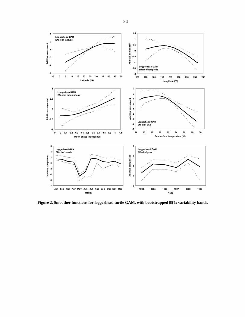
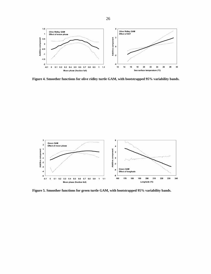
running under IRIX 6.5.4 on an SGI Challenge L workstation. Observer data (n=2,812 sets) and logbook data from un-observed trips (n=55,785 sets) from the years 1994-1998 were initially examined. A set of variables common to both the observer and logbook databases was evaluated in the GAMs: latitude, longitude, trip type, month, and year, as well as the added variables moon phase and satellite- measured SST. Stepwise procedures were used to identify variables with a statistically significant contribution toward predicting turtle take. The stepwise procedure starts out with a fully saturated model with all variables specified with smoother functions, then the model is simplified by eliminating variables or using linear functions instead of nonlinear smoother functions. The rearward stepwise approach is favored in this type of statistical model (Trevor Hastie, personal communication). The statistical criterion used for the automated acceptance or rejection of terms in the GAM is called the Akaike Information Criterion (AIC, see Akaike, 1974), which is a goodness of fit index penalized by the number of parameters in the model. Individual GAMs were run for each turtle species: loggerhead, leatherback, olive ridley, and green. Degrees of freedom in each smoother function were constrained (df=2) to eliminate extraneous curvature. The individual smoother functions for each of the final models are shown graphically in Figures 2-5. The final loggerhead GAM included smoothed nonlinear effects from latitude, longitude, moon phase, and SST, and categorical effects from each month and each year. The final leatherback GAM included smoothed nonlinear effects from latitude and moon phase, a linear effect from longitude, and categorical effects from each month. The final olive ridley GAM included a smoothed nonlinear effect from moon phase and a linear effect from SST. The final green GAM included a linear effect from longitude and a smoothed nonlinear effect from moon phase. These GAMs were used to make per-set take predictions across the entire logbook database using the selected variables for each turtle species. Exploratory plots summarizing turtle take by latitude, longitude, and month were created from the final turtle take database. Each GAM was bootstrapped 100 times using random permutations of the observer database, and the 95% variability bands were estimated from the distributions of the smoother functions (Efron & Gong, 1983). These nonparametric or empirical variability bands were constructed by sorting the binned smoother function values from low to high and using the 2.5%th and the 97.5%th values to identify the medial 95% of the distribution.

The logbook database of turtle take was then examined in a series of computer

simulations mimicking the effects of various protective management scenarios. Management scenarios were restricted to seasonal and spatial closures of the longline fishing grounds. Seasonal closures consisted of single month and adjacent multimonth closures spanning all possible combinations from 1 to 11 months in duration. Spatial closures consisted of latitudinal closures (i.e., “no fishing north of…”), longitudinal closures (i.e., “no fishing east of…”), and box closures, which combined the characteristics

5

of a latitudinal closure and a longitudinal closure. These constraints on fishing effort were chosen because of the predominantly northward and westward distributions of leatherback turtle take and the orientation of the fishing grounds with respect to the Hawaiian island chain; hence, spatial closures were examined at the resolution of whole degrees with “north of” values ranging from latitude 20°N to 40°N and “east of” values ranging from longitude 174° W to 145°W. Seasonal and spatial closures were combined in two possible ways with the first being a “separated” mode where the seasonal closure impacts all areas for the duration of the closed season, while the spatial closure is in effect for all time. The second type of seasonal and spatial closure combination is a “merged” mode, where the seasonal closure applies only to the spatial closure region. Similarly, the spatial closure is only for the duration of the seasonal closure. In any given management action simulation, fishing effort, fish catch, fish catch revenue, and turtle take of all species were tabulated under two modes of effort reallocation. In the “static” mode, fishing activity was assumed to not adjust after any management action, and any fishing effort lost because of spatial and/or seasonal closures was simply ignored. In the “dynamic” mode, the fishery was assumed to respond to the closures in a predictable manner. For spatial closures, it was assumed that complete spatial reallocation of lost fishing activity would occur, and this was modeled using monthly trip type-based expansions of open-area fishing activity. For seasonal closures, it was assumed that a maximum of one month’s fishing activity could be reallocated symmetrically to adjacent months bounding the seasonal closure; operationally this was approximated by allocating each lost set with a multiplier of 0.5/(number of closed months) to each bounding month. For this report, all years of data were combined to provide an average historical effect of a given management scenario. It should be noted that reallocation is based upon existing fishing patterns and this leads to several important points: 1) reallocation of fishing effort could possibly not occur, if there were no entries in the appropriate month-trip type-area strata, 2) unfished month-trip type-area strata would remain unfished; i.e., we do not account for possible expansion of the fishing grounds, and 3) management mechanisms currently in place and reflected in the data are accounted for in the reallocation; i.e., protective influences of the existing 50 nmi longline closures around the Northwestern Hawaiian Islands are retained, and all predicted changes from status quo are considered as supplemental to existing effects.

Fish catch revenue impacts of each closure scenario were calculated based upon the

values of individual fish kept or lost due to the closure. These data were made available from economic analyses of the pre-litigation longline fishery (Sam Pooley, personal communication). Ex-vessel prices ($/pound) and values ($/fish) were calculated for all major species by month and trip type (broadbill, mixed, tuna) for the 1998 fishing year by merging the NMFS sample of wholesale market prices with trips identified in the NMFS logbook reports for 1998. These values were applied to estimated catches in each time-area stratum to estimate ex-vessel revenues. The NMFS wholesale price sample was roughly 30%-35% of all longline transactions in 1998. Previous analysis has shown consistency with the Hawaii Division of Aquatic Resources longline price reports for recent years. Where no data were available for a species-month-trip type stratum, extrapolations for that month and species were used, weighted by annual average differences between trip types.

6

After accounting for all possible combinations of seasonal and spatial closures under separated, merged, static, and dynamic modes, a total of 361,194 possible management scenarios were evaluated. Evaluation was based on several important criteria such as percent change in turtle take by species, percent of fishing activity (longline gear sets) disrupted by the management action (i.e., static), percent of fishing activity lost after reallocation (i.e., dynamic), and percent change in fish catch revenue. For simplicity all scenarios were first partitioned into bins (e.g., 0%-5%, 5%-10%, 10%-15%, etc.) based upon values of the dynamic percent change in the take of leatherback turtles since this was the primary species of concern. Within these bins of leatherback take, the results were further sorted to discover optimal scenarios based on the criteria mentioned above, particularly the static value of fishing effort impact. This value of fishing effort disruption is an attractive criterion for gauging the impact of a time-area closure because it makes no assumptions about reallocation of lost fishing effort and is, therefore, useful in comparing different types of closure scenarios. We feel that fishing effort disrupted by a closure provides a basic measure of the impact of the closure because while it provides a measure of the fraction of effort impacted by the closure, it stops short of making further assumptions about how the fleet responds to that disruption and the economic impacts of this hypothetical response. At present, we are not confident we can model the fleet response and resulting economics with sufficient accuracy to determine the best closures; hence, fishing effort disruption remains the index value of choice. Several multicriteria optimizations were also attempted, such as simply summing static percent fishing activity lost and dynamic percent fishing activity lost to form a sum of percents. This particular optimization would search for a scenario with a minimal combined effect of disruption of fishing activity and net loss of fishing activity after adjustment to a seasonal or spatial closure. Another multicriteria optimization summed the individual turtle species’ take change together. This optimization would search for a scenario that best reduced the take of all turtle species, in an equally weighted fashion. A larger multicriteria optimization was formed by appropriately combining the two previously mentioned optimizations while paying close attention to arithmetic sign, so that the final criterion would both minimize disruption/loss while maximizing aggregate take reduction. For a given optimization, there were often many scenarios that nearly equally well met the optimization criteria, even at the resolution of whole degrees of latitude/longitude and whole months of time. The output from these exercises is voluminous, and it is difficult to select a clearly superior solution for a given optimization. Scenarios that differ in only a few percentage points are probably not significantly different from each other based upon some preliminary analyses of variability. For this reason, many scenarios should be evaluated together with additional input and criteria from fishermen, industry, and other concerned parties.

Variability of predicted turtle take was estimated by constructing 95% variability

bands around the values of interest using a randomization bootstrap procedure (Efron & Gong, 1983). In this procedure, individual longline sets in the observer database were randomly resampled with replacement to construct a new database of the original size. The GAMs were refitted with this new dataset and a new fleet-wide set of predicted turtle takes generated. This process was repeated 100 times and the distributions of the final values were used to address variability. The nonparametric or empirical variability bands were

7

constructed by sorting the values from low to high and using the 2.5%th and the 97.5%th values to identify the medial 95% of the distribution. This approach was also used to explore variability of the GAM smoother functions as described earlier and was here used to address variability of the optimal management scenarios for reducing leatherback sea turtle take.

The predicted effect of the emergency closure was examined using the same fleet-

wide turtle take database. This closure went into effect in November 1999 and closed the area north of latitude 28°N and between longitude 168°W and 150°W. The effects on turtle take, fishing effort, fish catch, and fish catch revenue were examined for this proposal under both static and dynamic reallocation modes. These results were compared to the results from the optimizations.

Lastly, the GAMs were refitted using a substantially larger amount of observer data

(12,688 sets vs initial 2,812 sets), made available from a longer time span of data collection and a sharply increased observer coverage in the longline fleet during recent years (Table 1). This represented an approximately 4.5X increase in the sample size. Each GAM was refit using the augmented data and monthly, latitudinal, and longitudinal summaries were compared to the initial analysis.

RESULTS AND DISCUSSION

The results of this report will focus on optimal time-area closures with emphasis on leatherback turtles. The exploratory graphical analyses (Figs. 6 and 7) indicated that April and May accounted for the highest monthly leatherback takes, with a relatively widespread spatial distribution. This is in contrast to olive ridleys and especially loggerheads, which have relatively well defined latitudinal ranges. Olive ridleys tend to be taken more in the southerly regions of the fishing grounds, while loggerheads are primarily taken in the northerly regions. Results from all scenarios are plotted graphically in Figure 8, using leatherback turtle take on the x-axis, and fishing effort disruption on the y-axis. This method of presenting the data is very similar to the “efficient frontier,” a financial concept used in Modern Portfolio Theory (Markowitz, 1991). The graph displays an envelope of points representing the hyperspace of possible outcomes. The efficient frontier is the point at which one quantity of interest is optimized at some preset value of another quantity of interest (in finance the plot would be of risk versus return). In Figure 8, fishing effort disruption is the quantity to be optimized, and the efficient frontier is the trace of points at the highest elevation for a given value of leatherback turtle take. Further examination of the management scenarios focused upon values along several of these efficient frontiers.

The five best scenarios per take reduction bin for each of the 10 different types of

management regimes are broken down in Figure 9 for leatherback turtle take and fishing effort disruption. This shows the performance and capability of various types of time or

8

area closures. Note that to achieve optimal solutions at high levels of turtle take reduction, separated mode combinations of seasonal and spatial closures are required. At lower levels of turtle take reduction, simpler merged-mode combinations or spatial closures only may be adequate. Generally, combinations of seasonal and spatial closures provide the best solutions when targeting a particular level of turtle take reduction, at least when best is defined as having the least disruption of fishing effort.

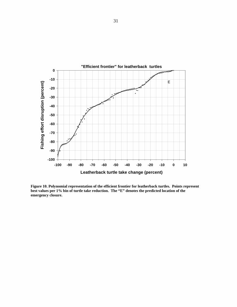
The efficient frontier margin for leatherbacks, estimated with a high degree

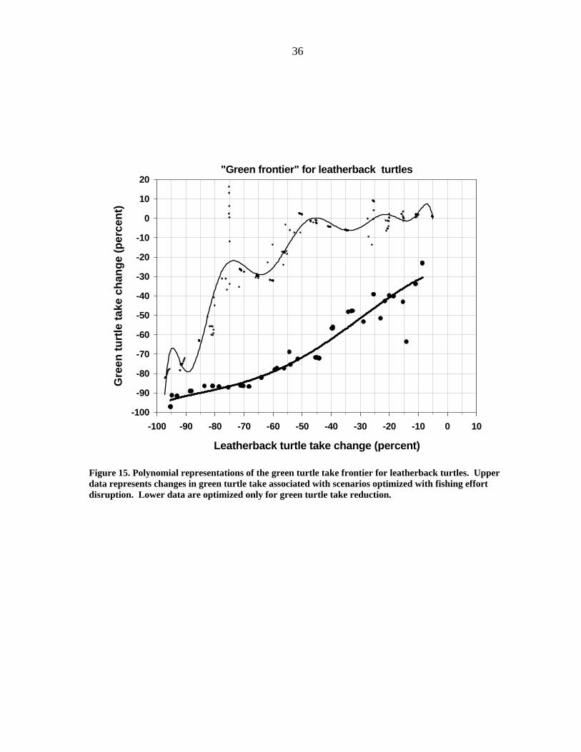
polynomial fit to 1% bin points, is shown in Figure 10. Variability along the leatherback turtle efficient frontier is shown in Figure 11, where each best scenario per 1% take bin is bootstrapped 100 times, with the medial 95% of values bounded by a variability band. This approach will allow construction of nonparametric or empirical variability bands around not only the efficient frontier but also any specific output for a given management scenario. Revenue values from the efficient frontier for fishing effort disruption are shown in Figure 12. Note that this plot does not show an efficient frontier since revenue was not the value under optimization (earlier attempts at this approach were unsuccessful due to unstable boundary solutions; i.e., proposing nearly 100% fishing effort disruption to inflate low sample size revenue values). This figure is presented to indicate how revenue is predicted to change for targeted levels of leatherback turtle take reduction at optimal values of fishing effort disruption. This is only revenue changes from changes in fish catch quantity and composition and does not include potential additional costs associated with compliance to a management scenario (e.g., transit costs, loss of fishing days). Figures 13-15 show how the takes of other turtle species change along the efficient frontier for leatherback turtle take and fishing effort disruption. These are also not true efficient frontiers since the take rates for loggerhead, olive ridley, and green were not optimized. These show predicted changes in take for other turtle species along the leatherback efficient frontier with respect to optimized fishing effort disruption. Figure 13 is particularly interesting because it highlights some closures that reduce leatherback takes and also substantially reduce loggerhead takes. Specifically for the closures that reduce leatherback takes by 20%-30% and by 50%-60% there are some closures that also reduce loggerhead takes by 40%-55% (Fig. 13). Additionally, the true efficient frontiers of other turtle takes are plotted on Figures 13-15; these are easily distinguished from the above by their relative smoothness and magnitude of turtle take reductions. These scenarios, however, tend to disrupt the fishery to a greater extent.

Table 3 shows the “best” results for all 19 bins by 5% leatherback turtle take

reduction. The optimization criterion in choosing these scenarios was to minimize disruption of fishing effort. Other criteria, including multicriteria, were attempted, but until they are better refined the simple disruption of fishing effort appears to provide the best optimization index. Some problems with the multicriteria optimizations included high fishing effort disruption balanced by an assumed complete spatial reallocation to a small area; this optimization needs to be constrained to minimize disruption and loss separately. Summing these two changes resulted in lost information content. The aggregated turtle take reduction optimization suffered from excessive weighting toward loggerhead solutions since these were the most easily reduced; again, summing the take changes

9

resulted in lost information content, and a penalty function for asymmetry may be the solution. For the fishing effort disruption criterion, even this small subset of the simulation output comprises 19 management scenarios, each one worthy of consideration for a particular level of targeted leatherback turtle take. These 19 scenarios represent the most efficient management actions to consider with regard to leatherback turtle protection. It is important to emphasize that many other unpresented scenarios may differ in only a degree of latitude or a degree of longitude or a single month yet fall upon a similar location on the efficient frontier. These subtle differences in management tactic may be very important from the perspective of a longline fisherman. For example, the transit time/expense for a single degree of latitude/longitude is nontrivial. If travel time increases by only a single day per trip, the net loss to a fisherman was estimated to be $4,000 per year in 1993 (Hamilton et al., 1996). The loss of a single day of fishing (i.e., approximately one longline set) per trip was estimated to incur an annual cost of $16,000. The predicted effects of the emergency closure for turtle take effects and fish catch effects are summarized in Tables 4A and 4B. Since this is a strictly spatial closure, the simulation reallocated 100% of the disrupted fishing effort to areas outside of the closure during the same months and same trip-type effort. Fish catch revenue references the total change using the entire catch, including many additional species not listed in the table. The effects are broken down by year and a multiyear average is presented at the bottom of each table. This scenario is predicted to be somewhat detrimental to olive ridley and green turtles, while producing a relatively small protective effect for leatherback turtles, the species for which it was originally intended. It disrupts approximately 13% of the fishing effort with a small decrease in fish catch revenue. The emergency closure scenario is quite distant to the efficient frontier for all species, when compared to other management scenarios found in Table 3 at this level of turtle take reduction. The symbol “E” is plotted on Figures 9-10 to indicate the predicted location of the emergency closure in comparison to the other scenarios. Table 5 lists 25 management scenarios that disrupt longline fishery effort to approximately the same extent as the emergency closure, but with more effective leatherback turtle take reduction. The GAM analyses appeared to be robust for all species since the monthly, latitudinal, and longitudinal summaries were similar between the initial runs and the 4.5X augmented data runs. This suggests that the spatial and temporal patterns identified in the initial modeling persisted as the sample size of the observer database grew from 2,812 sets to 12,688 sets. In particular, features such as the March-April pulse of leatherback takes appeared in both analyses (Fig. 16). Other spatial patterns in latitude (Fig. 17) and longitude (Fig. 18) were retained in both sets of take predictions, with a commensurate narrowing of the bootstrapped 95% variability bands as would be expected with a larger sample size. In conclusion, it has been shown that time-area closures are a viable option even in complex situations with multiple species of concern. The compromises in take reductions and impacts to fishermen can be quantitatively examined in a rigorous framework, which would assist fishery managers and protected resource managers in reaching consensus on

10

effective management measures acceptable to all constituents. The use of GAMs in processing observer data to identify important spatial and temporal patterns of sea turtle take is promising, and results appear to be robust with respect to sample size concerns. Further work in modeling pelagic movement as well as fishing gear characteristics will be a useful tool to assist in take mitigation.

ACKNOWLEDGMENTS

We thank Sam Pooley for providing the data necessary to estimate revenue impacts

in the time/area closure simulations, and for preparing the paragraph describing the data. Pierre Kleiber provided much-appreciated assistance with S-Plus GAM analysis and database preparation. We also thank Kathy Cousins, Charles Karnella, Pierre Kleiber, Mike Laurs, Marilyn Luipold, Alec MacCall, Marti McCracken, Rod McInnis, Dick Neal, Sam Pooley, Barbara Schroeder, Mike Tillman, and Jerry Wetherall for their helpful advice and reviews of earlier drafts of this report. The Time/Area Review Panel members Larry Crowder, John Hampton, and Mike Sissenwine offered helpful advice and constructive criticism as well.

11

REFERENCES

Akaike, H. 1974. A new look at statistical model identification. IEEE Transactions on Automatic Control. AU-19, 716-722.

Bearzi, G. 2002. Interactions between cetacean and fisheries in the Mediterranean Sea. In:

G. Notarbartolo di Sciara (Ed.), Cetaceans of the Mediterranean and Black Seas: state of knowledge and conservation strategies. A report to the ACCOBAMS Secretariat, Monaco, February 2002. Section 9, 20 p.

Bigelow, K. A., C. H. Boggs, and X. He. 1999. Environmental effects on swordfish and

blue shark catch rates in the US North Pacific longline fishery. Fish. Oceanogr. 3: 178-198.

Boggs, C. H. 2004. Pacific research on longline sea turtle bycatch. Pages 121-138 in Long,

K. J., and B. A. Schroeder (editors). Proceedings of the International Technical Expert Workshop on Marine Turtle Bycatch in Longline Fisheries. U. S. Dep. of Commer., NOAA Technical Memorandum NMFS-F/OPR-26, 189 p.

Bolten, A. B., and K. A. Bjorndal. 2002. Experiment to evaluate gear modification on rates

of sea turtle bycatch in the swordfish longline fishery in the Azores. NOAA Award Number NA96FE0393 Final Project Report. Archie Carr Center for Sea Turtle Research, Gainesville, Florida. 14 p.

Borchers, D. L., S. T. Buckland, I. G. Priede, and S. Ahmadi. 1997. Improving the

precision of the daily egg production method using generalized additive models. Can. J. Fish. Aquat. Sci. 54: 2727-2742.

Carreras, C., L. Cardona, and A. Aguilar. 2004. Incidental catch of the loggerhead turtle

Caretta caretta off the Balearic Islands (western Mediterranean). Biol. Conserv. 117(3): 321-329.

Chakravorty, U., and K Nemoto. 2001. Modeling the effects of area closure and tax

policies: a spatial-temporal model of the Hawaii longline fishery. Marine Resource Economics 15(3): 179-204.

Coles, W. C., and J. A. Musick. 2000. Satellite sea surface temperature analysis and

correlation with sea turtle distribution off North Carolina. Copeia 2: 551-554. Crowder, L. B. and R. A. Myers. 2001. A Comprehensive Study of the Ecological Impacts

of the Worldwide Pelagic Longline Industry. First Annual Report to the Pew Charitable Trusts. 31 December 2001. 166 pp.

Curtis, R., and R. L. Hicks. 2000. The cost of sea turtle preservation: the case of Hawaii’s

pelagic longliners. American Journal of Agricultural Economics 82(5): 1191-1197.

12

Dinardo, G. T. 1993. Statistical guidelines for a pilot observer program to estimate turtle takes in the Hawaii longline fishery. U.S. Dep. Commer., NOAA Tech. Memo. NOAA-TM-NMFS-SWFSC-190, 40 p.

Efron, B., and G. Gong. A leisurely look at the bootstrap, the jackknife, and cross-

validation. The American Statistician. 37(1): 36-48. Epperly, S. P., and C. Boggs. 2004. Post-hooking mortality in pelagic longline fisheries

using “J” hooks and circle hooks: application of new draft criteria to data from the Northeast distant experiments in the Atlantic. Southeast Fisheries Science Center, Protected Resources and Biodiversity Division. Internal document no. PRD-03/03-04. 8 p.

Forney, K. A. 2000. Environmental models of cetacean abundance: reducing uncertainty in

population trends. Conserv. Biol. 14:1271-1286. Goodyear, C. P. 1999. An analysis of the possible utility of time-area closures to minimize

billfish bycatch by U.S. pelagic longlines. Fish. Bull. 97: 243-55. Hamilton, M. S., R. E. Curtis, and M. D. Travis. 1996. Hawaii longline vessel economics.

Marine Resource Economics. 11(2): 137-140. Hastie, T. J., and R. J. Tibshirani. 1990. Generalized Additive Models. CRC Press. Boca

Raton, FL. 336 pp. Hays G. C., A. C. Broderick, B. J. Godley, P. Luschi, and W. J. Nichols. 2003. Satellite

telemetry suggests high levels of fishing-induced mortality in marine turtles. Mar. Ecol. Prog. Ser. 262: 305-309.

Ito, R. Y., and W. A. Machado. 2001. Annual report of the Hawaii-based longline fishery

for 2000. Honolulu Lab., Southwest Fish. Sci. Cent., Natl. Mar. Fish. Serv., NOAA, Honolulu, HI 96822-2396. Southwest Fish. Sci. Cent. Admin Rep. H-01-07, 39 p.

Jacobson, L. D., and A. D. MacCall. 1995. Stock-recruitment models for Pacific sardine

(Sardinops sagax). Can. J. Fish. Aquat. Sci. 52: 566-577. Kleiber, P. 1998. Estimating annual takes and kills of sea turtles by the Hawaiian longline

fishery, 1991-97, from observer program and logbook data. Honolulu Lab., Southwest Fish. Sci. Cent., Natl. Mar. Fish. Serv., NOAA, Honolulu, HI 96822-2396. Southwest Fish. Sci. Cent. Admin Rep. H-98-08, 21 p.

Kleiber, P. 1999. Estimated fleet-wide turtle takes and kill in the Hawaiian longline

fishery, 1994-1998. In: Pelagic Fisheries of the Western Pacific Region, 1998 Annual Report. Western Pacific Regional Fishery Management Council, Honolulu.

13

Knapp, R. A., and H. K. Preisler. 1999. Is it possible to predict habitat use by spawning salmonids? A test using California golden trout (Oncorhynchus mykiss aguabonita). Can. J. Fish. Aquat. Sci. 56: 1576-1584.

Kobayashi, D. R. and J. J. Polovina. 2001. Time/Area closure analysis for turtle take

reduction. Appendix C, Final Environmental Impact Statement, March 30, 2001, Fishery Management Plan - Pelagic Fisheries of the Western Pacific Region. URS Corporation, Honolulu, Hawaii. 45 p.

Kotas, J.E., S. dos Santos, V. G. Azevedo, B. M. G. Gallo, and P. C. R. Barata. 2004.

Incidental capture of loggerhead (Caretta caretta) and leatherback (Dermochelys coriacea) sea turtles by the pelagic longline fishery off southern Brazil. Fish. Bull. 102(2): 393-399.

Lewison, R. L., S. A. Freeman, and L. B. Crowder. 2004. Quantifying the effects of

fisheries on threatened species: the impact of pelagic longlines on loggerhead and leatherback sea turtles. Ecology Letters 7(3): 221-231.

Markowitz, H. M. 1991. Portfolio Selection: Efficient Diversification of Investments.

Blackwell Publishers. Oxford, U.K. 400 pp. McCracken, M.L. 2000. Estimation of sea turtle take and mortality in the Hawaiian

longline fisheries. Honolulu Lab., Southwest Fish. Sci. Cent., Natl. Mar. Fish. Serv., NOAA, Honolulu, HI 96822-2396. Southwest Fish. Sci. Cent. Admin Rep. H-00-06 29 p.

Nichols,W. J., A. Resendiz, J.A.Seminoff, and B. Resendiz. 2000. Transpacific migration

of a loggerhead turtle monitored by satellite telemetry. Bull. Mar. Sci. 67:937-47. Nitta, E. T., and J. R. Henderson. 1993. A review of interactions between Hawaii's

fisheries and protected species. Marine Fisheries Review 55(2): 83-92. NMFS 2001. Mortality of Sea Turtles in Pelagic Longline Fisheries Decision

Memorandum. February 16, 2001. Polovina, J. J., G. H. Balazs, E. A. Howell, D. M. Parker, M. P. Seki, and P. H. Dutton.

2004. Forage and migration habitat of loggerhead (Caretta caretta) and olive ridley (Lepidochelys olivacea) sea turtles in the central North Pacific Ocean. Fish. Oceanogr. 13(1): 36-51.

Polovina, J.J., E. Howell, D. M. Parker, and G. H. Balazs. 2003. Dive-depth distribution of

loggerhead (Carretta carretta) and olive ridley (Lepidochelys olivacea) sea turtles in the central North Pacific: Might deep longline sets catch fewer turtles? Fish. Bull. 101(1): 189-193.

14

Polovina, J. J., D. R. Kobayashi, D. M. Ellis, M. P. Seki, and G. H. Balazs. 2000. Turtles on the edge: movement of loggerhead turtles (Caretta caretta) along oceanic fronts, spanning longline fishing grounds in the central North Pacific, 1997-1998. Fish. Oceanogr. 9: 71-82.

Pritchard, P. C. H. 1996. Are leatherbacks really threatened with extinction? Chelonian

Conserv. Biol. 2(2): 303-305. Spotila, J.R., A.E. Dunham, A.J. Leslie, A.C. Steyermark, P.T. Plotkin, and F.V. Paladino.

1996. Worldwide population decline of Dermochelys coriacea: Are leatherback turtles going extinct? Chelonian Conserv. Biol. 2(2): 209-222.

Stoner, A. W., J. P. Manderson, and J. P. Pessutti. 2001. Spatially explicit analysis of

estuarine habitat for juvenile winter flounder: combining generalized additive models and geographic information systems. Mar. Ecol. Prog. Ser. 213: 253-271.

Swartzman, G., C. Huang, and S. Kaluzny. 1992. Spatial analysis of Bering Sea groundfish

survey data using generalized additive models. Can. J. Fish. Aquat. Sci. 49: 1366-1378.

Walsh, W. A., and P. Kleiber. 2001. Generalized additive model and regression tree

analyses of blue shark (Prionace glauca) catch rates by the Hawaii-based commercial longline fishery. Fish. Res. 53: 115-131.

Walsh, W. A., P. Kleiber, and M. McCracken. 2002. Comparison of logbook reports of

incidental blue shark catch rates by Hawaii-based longline vessels to fishery observer data by application of a generalized additive model. Fish. Res. 58: 79-94.

Watson, J. W., S. P. Epperly, A. K. Shah, and D. G. Foster. In Press. Fishing methods to

reduce sea turtle mortality associated with pelagic longlines. Can. J. Fish. Aquat. Sci.

Watters, G., and A. J. Hobday. 1998. A new measure for estimating the morphometric size

at maturity of crabs. Can. J. Fish. Aquat. Sci. 55: 704-714. Weimerskirch, H., N. Brothers, and P. Jouventin. 1997. Population dynamics of

Wandering Albatross Diomedea exulans and Amsterdam Albatross Diomedia amsterdamensis in the Indian Ocean and their relationships with long-line fisheries: Conservation implications. Biol. Conserv. 79: 257-270.

Witzell, W. N. 1999. Distribution and relative abundance of sea turtles caught incidentally

by the U.S. pelagic longline fleet in the western North Atlantic Ocean, 1992-1995. Fish. Bull. 97:200-211.

Work, T. M., and G. H. Balazs. 2002. Necropsy finding in sea turtles taken as bycatch in

the North Pacific long line fishery. Fish. Bull. 100:876-880..

15

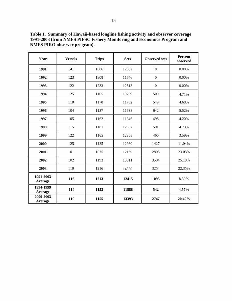
Table 1. Summary of Hawaii-based longline fishing activity and observer coverage 1991-2003 (from NMFS PIFSC Fishery Monitoring and Economics Program and NMFS PIRO observer program).

Year Vessels Trips Sets Observed sets Percent observed

1991 141 1686 12632 0 0.00%

1992 123 1308 11546 0 0.00%

1993 122 1233 12318 0 0.00%

1994 125 1105 10799 509 4.71%

1995 110 1170 11732 549 4.68%

1996 104 1137 11638 642 5.52%

1997 105 1162 11846 498 4.20%

1998 115 1181 12507 591 4.73%

1999 122 1165 12805 460 3.59%

2000 125 1135 12930 1427 11.04%

2001 101 1075 12169 2803 23.03%

2002 102 1193 13911 3504 25.19%

2003 110 1216 14560 3254 22.35%

1991-2003 Average 116 1213 12415 1095 8.39%

1994-1999 Average 114 1153 11888 542 4.57%

2000-2003 Average 110 1155 13393 2747 20.40%

16

Table 2. Summary of annual sea turtle take and mortality in the Hawaii-based longline fishery 1994-2002 (sea turtle takes from McCracken, personal communication; sea turtle mortality from Wetherall, personal communication).

Loggerhead Leatherback Olive Ridley Green Year Takes Mortality Takes Mortality Takes Mortality Takes Mortality

1994 501 202 109 36 107 52 37 16 1995 412 166 99 32 143 70 38 16 1996 445 178 106 35 153 74 40 17 1997 371 149 88 28 154 76 38 17 1998 407 164 139 47 157 80 42 18 1999 369 149 132 45 164 88 45 22 2000 246 106 132 45 113 65 65 35 2001 18 8 10 3 36 27 11 8 2002 17 7 5 2 31 29 3 3

1994-2002 Average 310 125 91 30 118 62 35 17 1994-1999 Average 418 168 112 37 146 73 40 18 2000-2002 Average 94 40 49 17 60 40 26 15

17

Table 3. “Best” scenarios optimized for minimal fishing effort disruption per 5% bin of leatherback turtle take reduction. Notations: LTTR = leatherback turtle take reduction 5% bin upper bound, #Mn = the number of months for a seasonal closure, Ms = the starting month of a seasonal closure, Lon/Lat = position of spatial closure, FED = fishing effort disruption, FEL = fishing effort lost, Rev = fish catch revenue change, Log = loggerhead turtle take change, Lea = leatherback turtle take change, Rid = olive ridley turtle take change, Gre = green turtle take change, Swo = swordfish catch change, Big = bigeye tuna catch change. Other fish species included in the revenue calculations are not presented.

LTTR

Type of management

action #Mn Ms Lon/Lat FED FEL Rev Log Lea Rid Gre Swo Big

-95%

Separated season latitude 9 11 37N -83.74% -73.03% -80.50% -90.17% -95.69% -59.98% -77.72% -91.30%

-76.27%

-90%

Separated season latitude 8 12 33N -76.98% -64.30% -74.84% -94.10% -90.50% -48.62% -72.00% -90.96%

-59.80%

-85% Separated season box 9 4 150W/32N -73.13% -63.69% -55.21% -36.31% -85.39% -74.87% -63.31% -61.67%

-60.34%

-80%

Separated season latitude 4 4 24N -58.84% -26.95% -36.91% -92.03% -80.44% 7.33% -40.79% -87.62%

-12.45%

-75%

Separated season latitude 4 4 31N -44.74% -26.95% -25.80% -46.54% -75.00% -21.38% -33.81% -48.50% -7.45%

-70% Separated season box 4 4 173W/33N -41.08% -26.95% -24.90% -16.17% -70.08% -25.78% -27.43% -36.11%

-10.48%

-65% Separated season box 4 4 157W/33N -38.72% -26.95% -25.89% 0.12% -65.00% -27.79% -30.01% -31.16%

-13.03%

-60%


-55% Separated season box 3 4 165W/33N -32.95% -19.00% -19.71% -15.08% -55.15% -14.54% -18.32% -27.08% -7.68%

-50%


18

Table 3. (Continued)

LTTR

Type of management

action #Mn Ms Lon/Lat FED FEL Rev Log Lea Rid Gre Swo Big -45%

Separated season box 2 4 171W/34N -23.93% -10.04% -10.25% -16.39% -45.01% -5.82% -2.59% -16.30% -3.21%



-30% Season 2 4 - -20.07% -10.04% -11.02% -2.19% -34.23% -7.78% -6.22% -11.33% -5.58%

-25%

Separated season latitude 1 4 33N -16.15% 0.00% 0.57% -32.68% -25.48% 6.14% -0.46% -11.79% 5.65%

-20%

Merged season latitude 11 9 31N -8.62% 0.00% 0.88% -35.26% -20.03% 5.84% 2.26% -15.67% 6.16%

-15%

Merged season latitude 4 9 31N -4.89% 0.00% 1.58% -20.19% -15.06% 5.05% -1.24% -10.43% 4.61%

-10% Merged

season box 2 11 170W/33N -2.81% 0.00% 0.71% -10.29% -10.11% 1.44% 1.90% -4.30% 2.09%

-5% Merged

season box 1 12 160W/33N -1.12% 0.00% 0.18% -0.48% -5.03% 0.39% 0.96% -1.14% 0.34%

19

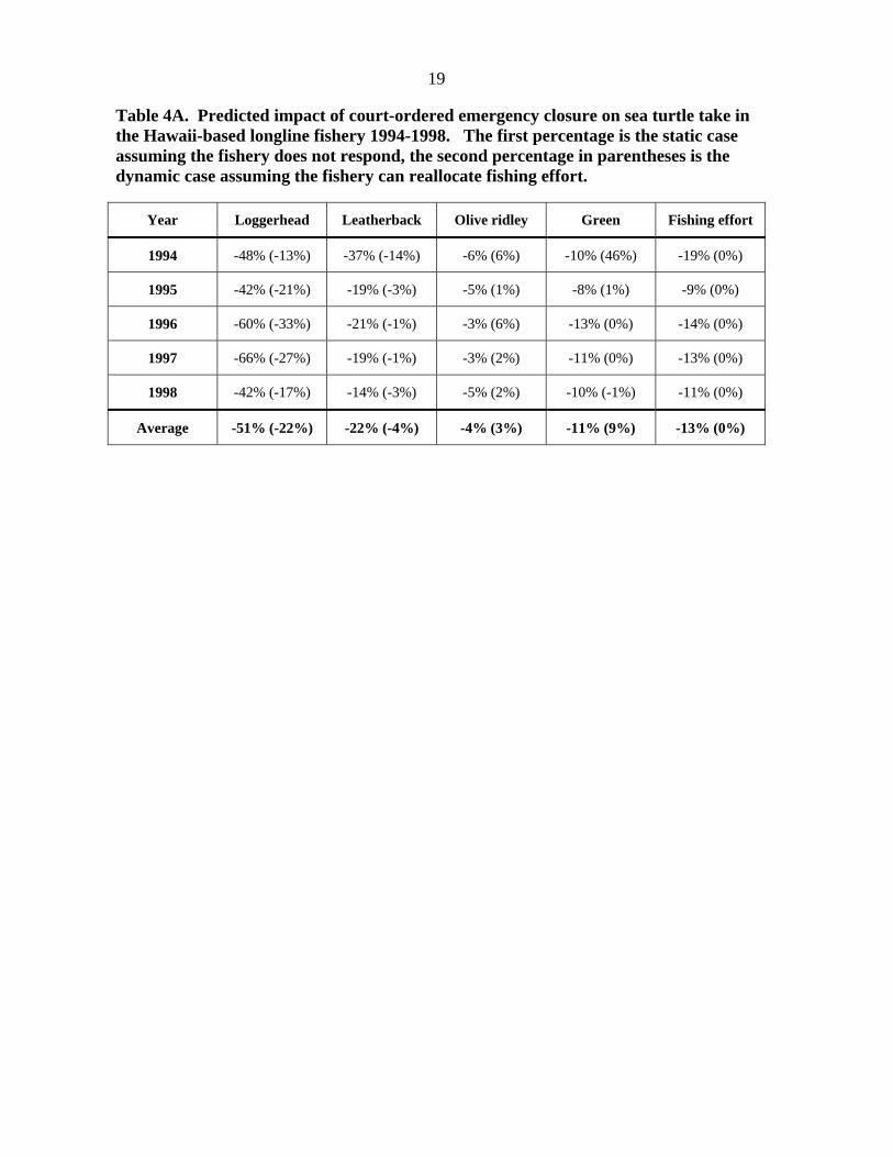
Table 4A. Predicted impact of court-ordered emergency closure on sea turtle take in the Hawaii-based longline fishery 1994-1998. The first percentage is the static case assuming the fishery does not respond, the second percentage in parentheses is the dynamic case assuming the fishery can reallocate fishing effort.

Year Loggerhead Leatherback Olive ridley Green Fishing effort

1994 -48% (-13%) -37% (-14%) -6% (6%) -10% (46%) -19% (0%)

1995 -42% (-21%) -19% (-3%) -5% (1%) -8% (1%) -9% (0%)

1996 -60% (-33%) -21% (-1%) -3% (6%) -13% (0%) -14% (0%)

1997 -66% (-27%) -19% (-1%) -3% (2%) -11% (0%) -13% (0%)

1998 -42% (-17%) -14% (-3%) -5% (2%) -10% (-1%) -11% (0%)

Average -51% (-22%) -22% (-4%) -4% (3%) -11% (9%) -13% (0%)

20

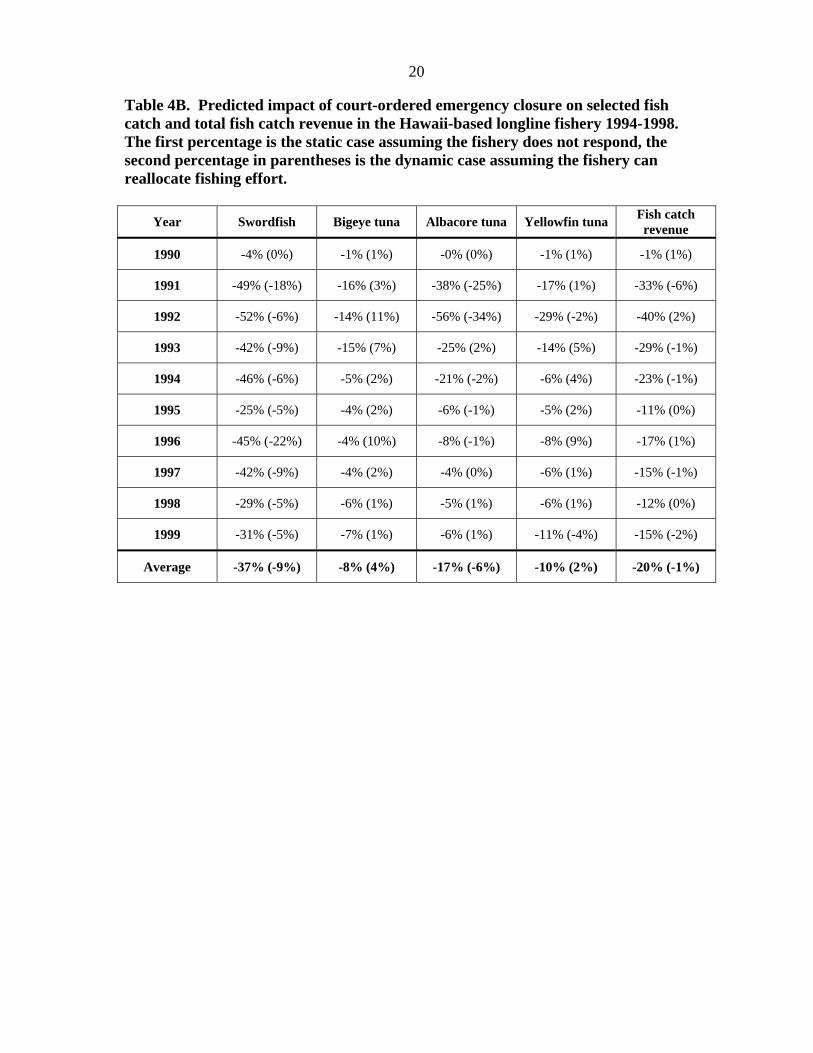
Table 4B. Predicted impact of court-ordered emergency closure on selected fish catch and total fish catch revenue in the Hawaii-based longline fishery 1994-1998. The first percentage is the static case assuming the fishery does not respond, the second percentage in parentheses is the dynamic case assuming the fishery can reallocate fishing effort.

Year Swordfish Bigeye tuna Albacore tuna Yellowfin tuna Fish catch

revenue

1990 -4% (0%) -1% (1%) -0% (0%) -1% (1%) -1% (1%)

1991 -49% (-18%) -16% (3%) -38% (-25%) -17% (1%) -33% (-6%)

1992 -52% (-6%) -14% (11%) -56% (-34%) -29% (-2%) -40% (2%)

1993 -42% (-9%) -15% (7%) -25% (2%) -14% (5%) -29% (-1%)

1994 -46% (-6%) -5% (2%) -21% (-2%) -6% (4%) -23% (-1%)

1995 -25% (-5%) -4% (2%) -6% (-1%) -5% (2%) -11% (0%)

1996 -45% (-22%) -4% (10%) -8% (-1%) -8% (9%) -17% (1%)

1997 -42% (-9%) -4% (2%) -4% (0%) -6% (1%) -15% (-1%)

1998 -29% (-5%) -6% (1%) -5% (1%) -6% (1%) -12% (0%)

1999 -31% (-5%) -7% (1%) -6% (1%) -11% (-4%) -15% (-2%)

Average -37% (-9%) -8% (4%) -17% (-6%) -10% (2%) -20% (-1%)

21

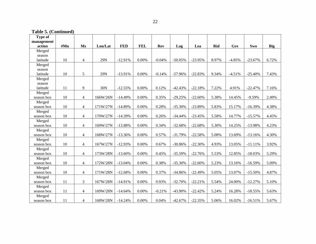
Table 5. Listing of twenty-five best scenarios for fishing effort disruption approximating Emergency closure effect (-10% to -15%) optimized for leatherback turtle take reduction. Notations: #Mn = the number of months for a seasonal closure, Ms = the starting month of a seasonal closure, Lon/Lat = position of spatial closure, FED = fishing effort disruption, FEL = fishing effort lost, Rev = fish catch revenue change, Log = loggerhead turtle take change, Lea = leatherback turtle take change, Rid = olive ridley turtle take change, Gre = green turtle take change, Swo = swordfish catch change, Big = bigeye tuna catch change. Other fish species included in the revenue calculations are not presented. Results are not presented in any ordered sequence.

Type of management

action #Mn Ms Lon/Lat FED FEL Rev Log Lea Rid Gre Swo Big Latitude 0 0 30N -13.54% 0.00% -0.26% -49.88% -22.23% 8.15% 2.82% -24.38% 7.22%

Separated season latitude 1 4 34N -14.77% 0.00% 0.21% -26.41% -22.18% 5.08% -0.96% -10.19% 4.78%

Separated season box 1 4 170W/33N -14.93% 0.00% 1.27% -20.67% -22.46% 3.44% 5.75% -6.81% 4.22% Separated season box 1 4 169W/33N -14.80% 0.00% 1.15% -19.85% -22.18% 3.32% 5.71% -6.53% 4.02% Separated season box 1 4 168W/33N -14.74% 0.00% 1.08% -19.70% -22.17% 3.25% 5.59% -6.37% 3.88%

Merged season latitude 7 7 26N -13.54% 0.00% -0.89% -54.36% -22.22% 16.00% -11.67% -23.96% 2.93% Merged season latitude 9 4 28N -13.60% 0.00% 0.51% -35.22% -23.67% 9.71% -8.45% -22.62% 4.34% Merged season latitude 9 5 27N -14.75% 0.00% -0.08% -52.63% -23.93% 11.51% -12.23% -23.58% 4.60% Merged season latitude 9 5 28N -12.64% 0.00% -0.02% -51.39% -23.05% 9.90% -8.99% -21.64% 4.99% Merged season latitude 9 6 28N -14.93% 0.00% -1.48% -64.37% -22.39% 10.57% -8.80% -27.76% 5.71%

22

Table 5. (Continued) Type of

management action #Mn Ms Lon/Lat FED FEL Rev Log Lea Rid Gre Swo Big Merged season latitude 10 4 29N -12.91% 0.00% -0.04% -50.05% -23.95% 8.97% -4.85% -23.67% 6.72% Merged season latitude 10 5 29N -13.91% 0.00% -0.14% -57.96% -22.83% 9.34% -4.51% -25.40% 7.43% Merged season latitude 11 9 30N -12.55% 0.00% 0.12% -42.43% -22.18% 7.22% 4.91% -22.47% 7.16% Merged

season box 10 4 166W/26N -14.49% 0.00% 0.35% -29.25% -22.60% 5.38% 14.45% -9.59% 2.49% Merged










season box 11 4 169W/28N -14.64% 0.00% -0.21% -43.90% -22.42% 5.24% 16.28% -18.55% 5.63% Merged

season box 11 4 168W/28N -14.24% 0.00% 0.04% -42.67% -22.35% 5.06% 16.02% -16.51% 5.67%

23

Figure 1. Map of Hawaii-based longline fishing effort (1994-1999).

24

Figure 2. Smoother functions for loggerhead turtle GAM, with bootstrapped 95% variability bands.

25

Figure 3. Smoother functions for leatherback turtle GAM, with bootstrapped 95% variability bands.

26

Figure 4. Smoother functions for olive ridley turtle GAM, with bootstrapped 95% variability bands.

Figure 5. Smoother functions for green turtle GAM, with bootstrapped 95% variability bands.

27

Turtle take in longline fishery by month (1994-1998)

MonthJan Feb Mar Apr May Jun Jul Aug Sep Oct Nov Dec

Perc

ent i

n m

onth

ly b

in

0

5

10

15

20

25 LoggerheadLeatherbackOlive RidleyGreen

Figure 6. Turtle take in the Hawaii-based longline fishery by month, 1994-1998.

28

Turtle take in longline fishery by latitude (1994-1998)

Latitude

0N 5N 10N 15N 20N 25N 30N 35N 40N 45N 50N

Perc

ent i

n on

e de

gree

bin

0

2

4

6

8

10

12

14

16

18

LoggerheadLeatherbackOlive RidleyGreen

Turtle take in longline fishery by longitude (1994-1998)

Longitude

170E 175E 180 175W 170W 165W 160W 155W 150W 145W 140W 135W

Perc

ent i

n on

e de

gree

bin

0

2

4

6

8

10

12

LoggerheadLeatherbackOlive RidleyGreen

Figure 7. Turtle take in the Hawaii-based longline fishery by latitude and longitude, 1994-1998.

29

Figure 8. All management scenarios evaluated in the leatherback turtle take reduction simulations, showing changes in turtle take and fishing effort disruption.

30

Five best scenarios per 5% take bin per type of regime

Leatherback turtle take change (percent)-100 -90 -80 -70 -60 -50 -40 -30 -20 -10 0

Fish

ing

effo

rt d

isru

ptio

n (p

erce

nt)

-100

-90

-80

-70

-60

-50

-40

-30

-20

-10

0

1 1

1 1

11

11

11

1

1

1

1

1

11

11

1

1

11

11

1

1

1

1

1

1

1

1 1

1

1

1 1

1

1

1

1

1

1

1

1

1

1

11

111

1

11

1

1

1

1

11

1 1

1

1

11

11

1

1

11

1

11

11

12

2 2 2 2

2

22

22

2

2

2

2

2

3 33

33

3

3

3

3

3

3

3

3

3

3

3

44444

44444

44 444

444 4

4

4

4444

4 4 4

4 444

44 44

4

4

4

4

55 55555 555

55555

555 55

5

5

555

55555

5

5

555

55555

6666666666

66666

6666

6

66666

6 6

66

6

6

6

6

6

6

7777777777

77777

777 77

77

777

77777

7

7

777

77777

88 8 8 8

8 8888

8 8 8 88

88

8

88

88

88

88 8

888

8

88 8 8

88 8 8 8

8

8

8 88

8888 8

8

8

888

8 8 88

8

8

8888

8

88

8 8

88888

88888

8888

8

88888

88888

9999 9

99999

9 9999

999 9

9

99

9

99

9

9

99

9

9 9 99

9

9

9

99

9

9

9 9 9

9

99

9

9

9

9

99

9

9

9

99

9 9

99

99

99

9

99 9

9

9

9

99

9

9

99

9

9999

9

99999

99999

10101010101010101010

1010101010

1010101010

1010101010

101010101010101010101010101010

1010101010

1010101010

1010101010

1010101010

10101010101010101010

101010

10

10

10

10

1010

10

1010101010

1010101010

1010101010

E

Season1

Longitude2

Latitude3

Merged season longitude4

Merged season latitude5

Box6

Merged season box7

Separated season longitude8

Separated season latitude9

Separated season box10

Emergency closureE

Figure 9. Best management scenarios evaluated in leatherback turtle take reduction simulations, broken down by type of management regime, changes in turtle take and fishing effort disruption. The “E” denotes the predicted location of the emergency closure.

31

"Efficient frontier" for leatherback turtles

Leatherback turtle take change (percent)

-100 -90 -80 -70 -60 -50 -40 -30 -20 -10 0 10

Fish

ing

effo

rt d

isru

ptio

n (p

erce

nt)

-100

-90

-80

-70

-60

-50

-40

-30

-20

-10

0

E

Figure 10. Polynomial representation of the efficient frontier for leatherback turtles. Points represent best values per 1% bin of turtle take reduction. The “E” denotes the predicted location of the emergency closure.

32

Variability of "efficient frontier" for leatherback turtles


-100 -90 -80 -70 -60 -50 -40 -30 -20 -10 0

Fish

ing

effo

rt d

isru

ptio

n (p

erce

nt)

-100

-90

-80

-70

-60

-50

-40

-30

-20

-10

0

Figure 11. 95% variability envelope of the efficient frontier for leatherback turtle take reduction and fishing effort disruption from bootstrapping.

33

"Revenue frontier" for leatherback turtles


-100 -90 -80 -70 -60 -50 -40 -30 -20 -10 0 10

Fish

cat

ch re

venu

e ch

ange

(per

cent

)

-100

-90

-80

-70

-60

-50

-40

-30

-20

-10

0

10

Figure 12. Polynomial representation of the revenue frontier for leatherback turtles. This represents the changes in fish catch revenue associated with scenarios optimized with respect to fishing effort disruption.

34

"Loggerhead frontier" for leatherback turtles


-100 -90 -80 -70 -60 -50 -40 -30 -20 -10 0 10

Logg

erhe

ad tu

rtle

take

cha

nge

(per

cent

)

-100

-90

-80

-70

-60

-50

-40

-30

-20

-10

0

10

Figure 13. Polynomial representations of the loggerhead turtle take frontier for leatherback turtles. Upper data represents changes in loggerhead turtle take associated with scenarios optimized with fishing effort disruption. Lower data optimized only for loggerhead turtle take reduction.

35

"Olive ridley frontier" for leatherback turtles


-100 -90 -80 -70 -60 -50 -40 -30 -20 -10 0 10

Oliv

e rid

ley

turt

le ta

ke c

hang

e (p

erce

nt)

-100

-90

-80

-70

-60

-50

-40

-30

-20

-10

0

10

20

Figure 14. Polynomial representations of the olive ridley turtle take frontier for leatherback turtles. Upper data represents changes in olive ridley turtle take associated with scenarios optimized with fishing effort disruption. Lower data optimized only for olive ridley turtle take reduction.

36

"Green frontier" for leatherback turtles


-100 -90 -80 -70 -60 -50 -40 -30 -20 -10 0 10

Gre

en tu

rtle

take

cha

nge

(per

cent

)

-100

-90

-80

-70

-60

-50

-40

-30

-20

-10

0

10

20

Figure 15. Polynomial representations of the green turtle take frontier for leatherback turtles. Upper data represents changes in green turtle take associated with scenarios optimized with fishing effort disruption. Lower data are optimized only for green turtle take reduction.

37

Figure 16. Sea turtle take (1994-1999) summarized by month for each species. The initial GAM predictions are on the left (n=2,812 sets) and the augmented-data GAM predictions are on the right (n=12,688 sets).

38

Figure 17. Sea turtle take (1994-1999) summarized by latitude for each species. The initial GAM predictions are on the left (n=2,812 sets) and the augmented-data GAM predictions are on the right (n=12,688 sets).

39

Figure 18. Sea turtle take (1994-1999) summarized by longitude for each species. The initial GAM predictions are on the left (n=2,812 sets) and the augmented-data GAM predictions are on the right (n=12,688 sets).

evaluation of time-area closures to reduce incidental sea

Documents