Master Thesis, 30 ECTS

M.Sc. Industrial Engineering and Management, 300 ECTS

Industrial Statistics and Risk Management

Spring 2021

EVALUATION OF THE

VARIANCE IN THE PREMIUM

PROVISION ESTIMATE

Handling Inhomogeneous and Decreasing Risk in Premium Provision Purposes

AUTHORS

Eric Egelius & Anna Methander

Copyright ©2021 Eric Egelius & Anna MethanderAll rights reserved.

EVALUATION OF THE VARIANCE OF THE PREMIUM PROVISION ESTIMATEHandling Inhomogeneous and Decreasing Risk in Premium Provision Purposes

Department of Mathematics and Mathematical StatisticsUmea University, Sweden

Supervisors:Hanna Magnusson, Anticimex InsuranceOleg Seleznjev, Umea UniversityGustav Tornqvist, Anticimex Insurance

Examiner:Leif Nilsson

Acknowledgements

We want to express our greatest gratitude to our supervisors at Anticimex Insurance,Gustav Tornqvist and Hanna Magnusson, for your valuable insights, supportive attitudeand open mindset. It has been a true privilege to have you as our supervisors. Thankyou!

The work process of this thesis has not been a straight path. We have had ups anddowns, highs and lows, but we do feel proud and cheerful that we now have brought it toa successful conclusion. Moreover, we want to thank Leif Nilsson, Program Director inUmea, for constantly develop the program and always care for the students.

Finally, we want to thank the persons that have contributed to the quality of the re-port by proofreading, among Emil Sandstrom, Ludvig von Schewelov and Oleg Seleznjev.Last but not least, thanks to our partners, Linn von Schewelov and Kristian Willman,for the unconditional support.

May 28th, 2021Stockholm

Eric Egelius & Anna Methander

i

Abstract

The costs related to events of losses within non-life insurance are stochastic and a pre-requisite of running a successful insurance business is to predict risks and future costs.From both a business- and regulatory perspective, it is of high interest to have a genuineunderstanding of the precision and the sensitivity of the estimated costs and future risks.This thesis aims to provide an alternative procedure of how to estimate the costs relatedto the future and, above all, the variance, in the case of dealing with inhomogeneous anddecreasing risk. The procedure is based on a separate modeling of the claim frequencyand the claim severity, that later can be combined to yield a total cost distribution fora determined time period. The claim severities are modeled based on a parametric anda non-parametric approach and the claim frequencies are modeled with the resamplingmethod bootstrap and by the use of scenarios. The thesis is made in collaboration withthe insurance company, Anticimex Insurance, who has contributed with the data as wellas expert knowledge related to the actuarial field. The results of the thesis show thatthe procedure is successful for evaluating estimated total costs distributions and theirfirst and second moments, even in the case of inhomogeneous and decreasing risk.

Keywords: Premium Provision, Reserves, Insurance, Claim Frequency,Inhomogeneous Risk, Claim Severity, Hidden Fault, Title Transfer Insurance.

Sammanfattning

Kostnader som uppkommer pa grund av skador inom skadeforsakring ar stokasiska ochen forusattning for att kunna bedriva ett framgangsrikt forsakringsbolag ar att kun-na prediktera risk och framtida kostnader. Utifran ett saval forsakrings- som reglato-riskt perspektiv ar det av stor vikt att ha en gedigen forstaelse av bade precisionenoch kansligheten i de skattade estimaten. Denna uppsats syftar till att ta fram ettalternativt tillvagagangssatt till hur kostnader relaterade till framtiden ska predikte-ras, med fokus pa att utvardera variationen i estimaten, vid fallet av en inhomogenoch avtagande risk. Tillvagagangssattet bygger pa en uppdelning mellan antalet ska-dor och kostnaden for skador, vilka modelleras separat for att sedan kombineras ochge en totalkostnadsfordelning for den avsedda tidsperioden. De historiska kostnadernamodelleras utifran ett parametriskt- och ett ickeparametriskt tillvagagangssatt. Ska-defrekvensen modelleras med hjalp av bland annat samplingsmetoden bootstrap samtgenom anvandandet av scenarier. Uppsatsen gors i samarbete med skadeforsakringsbo-laget, Anticimex Forsakringar, vilka har bidragit med data och expertkunskap inom detaktuariella omradet. Arbetets resultat visar att det foreslagna tillvagagangssattet aren framgangsrik strategi for att utvardera de forsta tva momenten av de predikteradetotalkostnadsfordelningarna, aven vid fallet av en inhomogen och avtagande risk.

Nyckelord: Premiereserv, Reserv, Forsakring, Skadefrekvens,Inhomogen Risk, Skadekostnad, Dolda Fel, Saljaransvarsforsakring.

ii

Contents

1 Introduction 21.1 Background . . . . . . . . . . . . . . . . . . . . . . . . . . . . . . . . . . . 2

1.1.1 Insurance . . . . . . . . . . . . . . . . . . . . . . . . . . . . . . . . 21.1.2 Reserving . . . . . . . . . . . . . . . . . . . . . . . . . . . . . . . . 3

1.2 Motivation and Approach . . . . . . . . . . . . . . . . . . . . . . . . . . . 31.3 Company and Project Description . . . . . . . . . . . . . . . . . . . . . . 4

1.3.1 Hidden Faults . . . . . . . . . . . . . . . . . . . . . . . . . . . . . . 51.3.2 Description and Problem Statement . . . . . . . . . . . . . . . . . 51.3.3 Confidentiality . . . . . . . . . . . . . . . . . . . . . . . . . . . . . 6

1.4 Outline . . . . . . . . . . . . . . . . . . . . . . . . . . . . . . . . . . . . . 7

2 Theory 82.1 Models for Claim Severity . . . . . . . . . . . . . . . . . . . . . . . . . . . 8

2.1.1 Log-normal Distribution . . . . . . . . . . . . . . . . . . . . . . . . 82.1.2 Gamma Distribution . . . . . . . . . . . . . . . . . . . . . . . . . . 92.1.3 Complications in Insurance Data . . . . . . . . . . . . . . . . . . . 9

2.2 Models for Claim Frequency . . . . . . . . . . . . . . . . . . . . . . . . . . 102.2.1 Bernoulli Distribution . . . . . . . . . . . . . . . . . . . . . . . . . 102.2.2 Binomial Distribution . . . . . . . . . . . . . . . . . . . . . . . . . 112.2.3 Poisson Distribution . . . . . . . . . . . . . . . . . . . . . . . . . . 11

2.3 Bootstrap . . . . . . . . . . . . . . . . . . . . . . . . . . . . . . . . . . . . 122.4 Stylized Scenarios . . . . . . . . . . . . . . . . . . . . . . . . . . . . . . . . 132.5 Law of Large Numbers (Weak) . . . . . . . . . . . . . . . . . . . . . . . . 132.6 Lyapunov Central Limit Theorem . . . . . . . . . . . . . . . . . . . . . . . 132.7 Pearson’s Chi-Square Test . . . . . . . . . . . . . . . . . . . . . . . . . . . 14

3 Methodology 163.1 Data . . . . . . . . . . . . . . . . . . . . . . . . . . . . . . . . . . . . . . . 16

3.1.1 Data Preprocessing - Product A . . . . . . . . . . . . . . . . . . . 163.1.2 Data Preprocessing - Product B . . . . . . . . . . . . . . . . . . . 213.1.3 Specific Data Adjustments for Product B . . . . . . . . . . . . . . 23

3.2 Method . . . . . . . . . . . . . . . . . . . . . . . . . . . . . . . . . . . . . 253.2.1 Software . . . . . . . . . . . . . . . . . . . . . . . . . . . . . . . . . 25

3.2.2 Claim Frequency Following a Poisson Distribution . . . . . . . . . 253.2.3 Risk of Claims . . . . . . . . . . . . . . . . . . . . . . . . . . . . . 283.2.4 Scenario Analysis of Claim Frequency . . . . . . . . . . . . . . . . 313.2.5 Allocate Underwriting Date . . . . . . . . . . . . . . . . . . . . . . 323.2.6 Cost of Claims . . . . . . . . . . . . . . . . . . . . . . . . . . . . . 32

4 Results 364.1 Validate Poisson Assumption . . . . . . . . . . . . . . . . . . . . . . . . . 364.2 Risk Curves . . . . . . . . . . . . . . . . . . . . . . . . . . . . . . . . . . . 37

4.2.1 Product A . . . . . . . . . . . . . . . . . . . . . . . . . . . . . . . . 374.2.2 Product B . . . . . . . . . . . . . . . . . . . . . . . . . . . . . . . . 38

4.3 Claim Frequency . . . . . . . . . . . . . . . . . . . . . . . . . . . . . . . . 404.3.1 Perspective 1 . . . . . . . . . . . . . . . . . . . . . . . . . . . . . . 404.3.2 Perspective 2 . . . . . . . . . . . . . . . . . . . . . . . . . . . . . . 404.3.3 Perspective 3 . . . . . . . . . . . . . . . . . . . . . . . . . . . . . . 41

4.4 Cost of Claims . . . . . . . . . . . . . . . . . . . . . . . . . . . . . . . . . 424.4.1 Product A . . . . . . . . . . . . . . . . . . . . . . . . . . . . . . . . 424.4.2 Product B . . . . . . . . . . . . . . . . . . . . . . . . . . . . . . . . 43

4.5 Total Cost Distribution . . . . . . . . . . . . . . . . . . . . . . . . . . . . 454.5.1 Perspective 1 . . . . . . . . . . . . . . . . . . . . . . . . . . . . . . 454.5.2 Perspective 2 . . . . . . . . . . . . . . . . . . . . . . . . . . . . . . 494.5.3 Perspective 3 . . . . . . . . . . . . . . . . . . . . . . . . . . . . . . 53

5 Discussion and Conclusions 585.1 General Comments . . . . . . . . . . . . . . . . . . . . . . . . . . . . . . . 58

5.1.1 Poisson Assumption . . . . . . . . . . . . . . . . . . . . . . . . . . 585.1.2 Claim Frequency . . . . . . . . . . . . . . . . . . . . . . . . . . . . 585.1.3 Cost of Claims . . . . . . . . . . . . . . . . . . . . . . . . . . . . . 595.1.4 Total Cost Distribution . . . . . . . . . . . . . . . . . . . . . . . . 60

5.2 Conclusions . . . . . . . . . . . . . . . . . . . . . . . . . . . . . . . . . . . 615.2.1 Final Models . . . . . . . . . . . . . . . . . . . . . . . . . . . . . . 61

5.3 Recommendations . . . . . . . . . . . . . . . . . . . . . . . . . . . . . . . 62

Appendices 65

A Product A 66

B Product B 68

Glossary

• ClaimA coverage request by a policyholder to the insurance company, in the event of ahidden fault. The claim can result in a

– Nil claim, if it does not result in a payment for the company.

– Non-nil claim, if it results in a payment for the company.

• Total Cost DistributionThe total cost and its estimated parameters for a determined amount of contractsand at a given time period.

• ReserveAlso known as technical provisions, which overall consists of the premium provisionand the claims provision. The reserve is the amount of funds required to cover theinsurance company’s undertakings and can be interpreted as a collateral. The totalcost distribution works as an input to the reserve calculations.

• Underwriting YearThe year of which the contract is written.

• Development YearThe number of years the contract has developed, after its underwriting. The under-writing year corresponds to the development period [0,1) and hence developmentyear 0. The year after the underwriting year corresponds to development year 1,and so forth.

• Accident YearThe year of which a fault has occurred. In this project, the occurrence is set tothe time the fault is detected by the buyer.

1

1. Introduction

This chapter serves as an introduction to the actuarial area and describes the specificreserving methods that are used today and the problems those methods encounter. There-after, the company behind this thesis is introduced together with a further description ofthe title transfer insurance contacts, the focus area of this thesis. Lastly, the structureoutline of this thesis is presented to the reader.

1.1 Background

1.1.1 Insurance

Insurance companies provide risk management to individuals, companies and institu-tional clients through contracts in order to protect against unexpected events. Thoughthere are multiple different types of insurance companies, the basic principal of insur-ance is to pool risks so that each policyholder shares the risk with a collective. Eachpolicyholder then pays a premium, that reflects the risk the policyholder adds to thecollective which, thanks to the pooled risk, is an affordable rate. Then, in the event oflosses, the insurer pays a reimbursement to the insured (Aviva, 2021). The insurancecompany does not know if a reimbursement will be made to a policyholder, how large thereimbursement will be and when in time it will occur. The potential costs are stochasticand infer uncertainty to the business and have to be assessed and evaluated from a sci-entific perspective. This is the job of an actuary. An actuary needs a strong backgroundin statistics, mathematics and business and needs to pass a series of exams to become acertified professional. The actuary’s job includes assisting in the scientific analysis andquantification of risks to evaluate the current financial implications of contingent eventsin the future, primarily by using probability- and economic theory and computer science.The convergence of those fields is called actuarial science (U.S. Bureau of Labor Statis-tics, 2021). According to the International Actuarial Association (2013), the actuarialknowledge should include expertise in developing and applying statistical- and financialmodels, as well as setting capital requirements, pricing and establishing the amount ofliabilities for uncertain future events.

2

1.1.2 Reserving

Every non-life insurance company must set up a reserve that covers the costs for con-tracts already entered to lower the risk of insolvency. This reserve can be divided intotwo parts: one part that covers the costs related to events that have occurred and onepart that covers the costs related to events that have not yet occurred, but for contractsalready entered. These parts are denoted the claims provision and the premium provi-sion, respectively, and consist of more than claims (Ohlsson, 2017). However, when theclaims- and premium provision are referred henceforth, only the claims’ part of thosereserves is considered. The scope of this project only includes the premium provision.

As previously stated, the premium provision considers events that have not yet hap-pened, but might occur in the future lifetime of the contracts. It is of great importancethat the insurance company has sophisticated estimates of how the costs related to con-tracts already entered will develop. The insurance company’s reserves must be carefullycalculated so that the company can meet their undertakings related to the outstand-ing contracts. However, it is of importance not to have too much excess capital in thereserves, since the money could be better used in other purposes, where the potentialreturn on the investment is higher. Since the reserves usually constitute a large share ofthe insurance company’s total holdings, even a small miscalculation of the reserve esti-mates can lead to a considerable large share of money (Bjorkwall, 2011). Therefore, it isfrom both a business strategic perspective and a regulatory perspective of high interestto know the precision and the sensitivity of the estimates.

1.2 Motivation and Approach

One of the most well-known methods used for estimating outstanding liabilities in non-life insurance is the Chain Ladder method (CLM). This method is a purely deterministicmethod based on finding representative development factors between time periods andis based on the assumption that prior patterns of losses will persist in the future. Itwas developed during a time when simple, closed-form expressions were important sincecomputers were not readily available. Since then, a lot of articles have been publishedshowing how these estimates are related to classic probability theory and more precisely,maximum likelihood theory. In 1991, Mack showed that the development factors of theCLM are maximum likelihood estimators of a multiplicative Poisson model (Martınez-Miranda, Nielsen and Verrall, n.d.). In 1993, Mack showed how the mean-squarederror of the Chain Ladder predictors could be calculated analytically (Mack, 1993) andin 1998, Renshaw and Verrall showed how Mack’s multiplicative Poisson model of thedevelopment factors could be extended to an over-dispersed Poisson model. These worksresulted therefore in some mathematical statistics of the CLM, while still maintainingthe simplicity and intuitiveness of the method (Bjorkwall, 2011).

A typical way to perform the reserving analysis is by using run-off triangles wheredevelopment factors are applied. Those triangles show how, e.g., the claim severityor the claim frequency develop over time, see Table 1.1 for an illustrative picture. Inaccordance with the notations used in Bjorkwall (2011), let the set {Cti; t, i ∈ ∇} denote

3

the incremental triangle of non-nil claims where ∇ = {t = 1, . . . T ; i = 0, . . . , T − t}. Thesuffixes t and i refer to the underwriting year and development year, respectively. Notethat the diagonals of ∇, i.e., t + i, represent the calendar years. In order to obtain anestimate of the reserve in accordance with this procedure, the lower, unobserved, futuretriangle {Cti; t, i ∈ ∆} where ∆ = {t = 1, . . . T ; i = T − t+ 1, . . . , T} must be predicted.

The company behind this project estimates the premium provision by using themethodology presented above, with starting point in either underwriting year or ac-cident year. Then, a prediction of the total reserve and the claims provision can beretrieved, respectively. By subtracting the estimate of the claims provision from the to-tal reserve and further correct for payments already made, an estimate of the premiumprovision is obtained. The major problem the actuarial team at the company encounterwhen retrieving the premium provision by the triangular approach is how to evaluatethe amount of variance appurtenant to the premium provision. Note that the approachresults in a dependency between the prediction of the premium provision and the claimsprovision and a distinct variance measure that corresponds to each of the reserves is notobtained, unless far-reached assumptions, e.g., equal uncertainty of both reserves, aremade. From a business perspective, it is of high importance to have a broad understand-ing regarding future costs related to the contracts already entered, where the first andsecond moments, i.e., the expected value and the variance, of the premium provision’sprobability distribution can be considered fundamental. Therefore, this thesis will pro-pose an alternative approach of how to estimate the premium provision in the case ofinhomogeneous and decreasing risk, where further the second moment of the premiumprovision’s probability distribution can be obtained.

Table 1.1: Incremental triangle of the observed claim severity {Cti; t, i ∈ ∇} where∇ = {t = 1, . . . T ; i = 0, . . . , T − t} and t is the year of underwriting and i is the year ofdevelopment.

Development YearUnderwriting Year 0 1 . . . T-1 T

1 C1,0 C1,1 · · · C1,T−1 C1,T

2 C2,0 C2,1 · · · C2,T−1

......

...T-1 CT−1,0

T CT,0

1.3 Company and Project Description

Anticimex Insurance is a subsidiary to Anticimex Group, the service company, and is amarket leader insurance company within the area of pest solutions and building environ-ments. Approximately 1’250 million SEK in yearly revenue makes Anticimex Insurancethe largest pest insurer in the world (Anticimex Insurance, 2019). A considerable part

4

of Anticimex Insurance business consists of title transfer insurance related to real prop-erty. There are multiple versions of those insurance contracts and the versions coverdifferent parts, but with the similarity that they all concern hidden faults govern by theLand Code. For analytical purposes, those contracts are partitioned into two productcategories, henceforth referred to Product A and Product B, where the insurance coverfor Product A is more extensive than it is for Product B. The Swedish law, Land Code(1970:994), governs hidden faults regarding real property. Chapter 4, 19§ specifies thatif the real property does not comply with the provisions of the agreement or if it de-viates from what the buyer could have presupposed at the time of the transaction, thebuyer has the right to make a deduction of the purchasing price. In reality, this is anindemnity paid out after the real property transaction is complete. Further, the buyerhas the right to a compensation for the costs related to the remedy of the hidden faultand the seller of the real estate is accountable for hidden faults in ten years from thetransaction time (SFS 1970:994). By entering a title transfer contract with AnticimexInsurance, the seller is, to a large extent, insured to potential costs related to hiddenfaults of the real property during the ten-year period by transferring this obligation toAnticimex Insurance.

1.3.1 Hidden Faults

A hidden fault is a fault that existed in the property at the time of the purchase that couldnot be detected, neither by the buyer nor by an inspection technician. Furthermore, thefault could not be expected based on a number of parameters, amongst age, conditionand price. Misunderstandings of how the concept hidden fault should be interpreted arecommon, since many people have heard about it, but might not have a full understandingof how to interpret it.

The age of the real estate is a vital factor for determining whether it concerns ofa hidden fault or not. A guideline is that the older the real estate is, the more faultsare expected and should have been taken into account by the buyer and are thereforeoften not considered hidden faults. If a fault is found in a new real estate, that couldnot be found at the time of the purchase, it can probably be considered a hidden fault(Anticimex, 2018).

One example of a hidden fault is an incorrectly executed drainage. Another is anewly laid roof with missing roofing felt on a smaller surface, which then leads to amoisture damage. For both to be classified as a hidden fault, they should not have beennoted during an inspection (Anticimex, n.d.). Note that both Product A and ProductB cover the parts described, but Product A further comprises some additional parts.

1.3.2 Description and Problem Statement

At the end of each fiscal year, Anticimex Insurance has active revenue-recognized con-tracts for ten underwriting years, which have been observed for various amount of time.The risk that a policyholder will report a claim differs depending on the remaining timeof the contract. To clarify: a contract that has been active for, e.g., nine years can be

5

considered less risky than a newly written contract. Partly because the remaining timeis shorter, but also because it becomes more difficult to show that a fault existed beforethe purchase. Therefore, a new cohort can be considered more uncertain than the olderones.

Further, as mentioned in Section 1.3, the title transfer insurance is for analyticalreasons divided into two product types. Due to the products’ structural differences, theamount of data differs between them, which further entails uncertainty.

The major focus of this thesis is to evaluate the variance of the total cost distributionfor both product types. To do so, an alternative approach to the one Anticimex applies,that separates the claims- and premium provision from one another, is suggested. Thisenables a retrievement of a more reliable variance measure for the total cost distributions.For each of the two products, the following will be estimated, by applying the suggestedapproach

• The total cost distribution for contracts with underwriting year 2021.

• The total cost distribution for accident year 2021.

• The total cost distribution for all active contracts.

Those three assignments are described in detail in Section 1.4 and are henceforth referredto as Perspective 1, 2 and 3, respectively.

The undertaking of this assignment will be made in collaboration with the actuarialteam at Anticimex Insurance. Further, the last observed date in the data is 2020-12-31and when referring to active contracts, it is the contracts that were active in this datethat are referred.

1.3.3 Confidentiality

Due to the sensitive nature of the data, a confidentiality agreement has been signedby both parties. This report is a limited version of the full report, where informationregarding the remaining risk of a claim, the claim frequencies, the claim severities andthe total cost distributions has been censured. The tables where results related to thoseareas are presented, are benchmarked with respect to a specific approach and method.For the remaining risk of a claim, the chosen benchmark is normalized to 1, and for theclaim frequencies and the total cost distributions, they are normalized to 100. Further,one of the axis in the figures is often removed, so that information regarding costs cannotbe retrieved. However, it will be pointed out clearly in the caption of the figures andtables if they have been normalized. Lastly, some results have been censored and arethus covered by black boxes.

All information and results have been approved by Anticimex Insurance before pub-lishing.

6

1.4 Outline

The thesis is structured as follows. In Chapter 2, a theoretical framework that gives thereader a relevant background to the reserving area, with focus on distribution functionsand statistical methods, is presented. In Chapter 3, the company data of the title transferinsurance contracts is introduced together with the preliminary data analyses and dataadjustments. Those analyses aim to give the reader a wider understanding of the twoproducts, so that the latter applied methods and procedures perceive straightforward.The chapter contains many algorithms and in order to make it easier for the reader tounderstand the chosen approaches, the algorithms are written in a mixture of descriptivetext, mathematical symbols and pseudocode. In Chapter 4, the results from the above-applied methods are presented and visualized. First, a visualization of the validation ofthe distribution functions is presented together with some test statistics. Thereafter, theresults for the following perspectives and/or the two products are presented separately.The perspectives are

• Perspective 1The first perspective refers to the expected claim frequency and claim severity forall contracts with underwriting year 2021. This includes estimating the numberof contracts for year 2021 and the remaining risk associated with those contracts.For an insurance company, this is important information for reinsurance purposesand for the general pricing of the products.

• Perspective 2The second perspective refers to the expected claim frequency and claim severityrelated to accident year 2021. This includes all currently active contracts andthose that will be written in year 2021. This perspective is important for regulatorypurposes, such as Solvency 2, where the capital requirements are determined on a99.5% value-at-risk measure over one year.

• Perspective 3The third perspective refers to the expected claim frequency and claim severity forall currently active contracts, when standing in 2020-12-31, that will occur duringthe remaining time of these contracts. The result from this perspective givesvaluable information about the company’s business, in terms of e.g. future costsand the company’s risk appetite.

Further, for each perspective and/or product, a parametric and a historic approachare applied together with three risk methods: Single Risk, Bootstrap and Scenario. InChapter 5, the results are discussed, conclusions are made and recommendations tofurther studies are suggested.

7

2. Theory

In this chapter, a theoretical framework covering the distribution functions used, generalcomplications in insurance data, algorithms, statistical tests and theorems are presented.The chapter aims to give the reader a theoretical understanding of the concepts andmethods later used in the thesis.

2.1 Models for Claim Severity

Within non-life insurance a common approach is to fit a probability density function tothe claim severity for a certain insurance type. A common feature of claim severitiesis that a small proportion of the claims constitutes a large proportion of the total cost.Therefore, long-tailed distributions often describe the data well (Johansson, 2014). Apresupposition in this section is that the claim severities are independent and equallydistributed stochastic variables.

2.1.1 Log-normal Distribution

A log-normally distributed stochastic variable can be written as eX , where X is a nor-mally distributed random variable with expected value µ and standard deviation σ.Thus, the variable (X − µ)/σ has expected value 0 and standard deviation 1, which isa standard normally distributed random variable. The probability density function of alog-normally distributed stochastic variable is defined as

f(x) =

{1√

2πσxexp

{− (lnx−µ)2

2σ2

}, x > 0,

0, x ≤ 0.

Expected Value

The expected value of a log-normally distributed random variable is

E[X] = exp

(µ+

σ2

2

).

8

Variance

The variance of a log-normally distributed random variable is

Var[X] =(

exp (σ2)− 1)

exp (2µ+ σ2).

2.1.2 Gamma Distribution

The probability density function of the gamma distribution is defined as

f(x;α, β) =

{βα

Γ(α)xα−1e−βx, x > 0,

0, x ≤ 0,

where Γ denotes the gamma function

Γ(α) :=

∫ ∞0

xα−1e−xdx,

with α > 0 and β > 0, where α is known as the shape parameter and β is known asthe inverse scale parameter or the rate parameter, where β = 1/θ and θ is the scaleparameter. The cumulative distribution function of a gamma distribution is defined as

F (y) =

∫ y

0

βα

Γ(α)xa−1e−βxdx.

The gamma distribution can further be adjusted in its horizontal location with thelocation parameter, µ. When µ = 0, it is usually referred to as ”the” gamma distribution(Wolfram Research, 2016).

Expected Value

If X has an absolutely continuous gamma distribution with probability density functionf, the expected value is

E[Xk]

=Γ(α+ k)

Γ(α)βk, k ≥ 0.

Variance

The variance of a gamma distributed random variable is

Var[X] =α

β2.

2.1.3 Complications in Insurance Data

In the following section, two frequently occurring complications in insurance data aredescribed.

9

Accretion of Costs

According to Johansson (2014), there are tendencies of rounding costs to even amounts,e.g., even thousands, which results in accretions of certain numbers. If the costs theretoare estimates of future payments, which often is the case for recently reported damages,this is even more frequently occurring. If the latter is the reason, there is no purposeof modeling these exact costs since they most probably will not be the final costs. Ifthe former is the case and if the accretions are modeled, the models will become toocomplicated.

Mixed Distributions

Sometimes it can be difficult to find a distribution that fits the entire data and a mixeddistribution can then be a proper choice. Johansson (2014) states an example whenmixed distributions are needed. The example is related to fire damage costs, where theinsurance payout is low if the fire was put out in an early stage and high if the fire tookhold and spread. Those costs could preferably be modeled with a mixed distribution.

A mixed distribution can be described as follows. Let X denote the cost for anarbitrary claim and let q denote the probability of a large claim (fire took hold andspread). Further, let the small claims follow the distribution G and the large claims thedistribution H. Then, X follows the distribution

F (x) = P (small damage) ∗ P (X ≤ x|small damage)+

P (large damage) ∗ P (X ≤ x|large damage) = (1− q)G(x) + qH(x).

Furthermore, note that a mixed distribution can contain of more than two distribu-tions.

2.2 Models for Claim Frequency

In the following section, let X denote a stochastic variable describing the number ofdamages affecting an insurance product. Moreover, all the distributions included in thissection are not used in the project, but are described in order to derive the later applieddistribution.

2.2.1 Bernoulli Distribution

The Bernoulli distribution is a special case of the binomial distribution (see definitionin Section 2.2.2). The Bernoulli distribution is a discrete distribution with two possibleoutcomes: k = 1 with probability p and k = 0 with probability q = 1 − p, where{p ∈ R : 0 ≤ p ≤ 1}. The probability mass function is defined as

Pr(k) = pk(1− p)(1−k).

A Bernoulli distributed random variable has expected value E[X] = p and varianceVar[X] = p(1 − p). Bernoulli trails are known as the performance of a fixed number oftrails and with a fixed probability of success in each trail.

10

2.2.2 Binomial Distribution

The binomial distribution is a discrete probability distribution with parameters n and p,modeling the number of successes in a sequence of n independent Bernoulli trails. Theoutcome from each experiment is either a success, with probability p, or a failure withprobability q = 1− p.

If X follows a binomial distribution with n ∈ N+, it is denoted as

X ∼ B(n, p).

The probability mass function of X describes the probability of getting exactly ksuccesses in n independent Bernoulli trails for k = 1, . . . , n and is given by

f(k, n, p) = Pr(X = k) =

(nk

)pk(1− p)n−k,

and where (nk

)=

n!

k!(n− k)!.

Expected Value

The expected value of X ∼ B(n, p) can be found by using the fact that X is the sum of nidentical Bernoulli random variables with the same probability, p. So, if X1, . . . , Xn areindependent and identically distributed (i.i.d) Bernoulli random variables with expectedvalue p, then

E[X] = E [X1 + . . .+Xn] = E [X1] + . . .+ E [Xn] = p+ · · ·+ p = np.

Variance

The variance of X ∼ B(n, p) can be found by using the fact that X1, . . . , Xn are i.i.d.Bernoulli random variables with expected value p, and X = X1, . . . , Xn, then the factthat the variance of a sum of i.i.d. random variables is the sum of variances can be used.It follows that

Var[X] = np(1− p).

2.2.3 Poisson Distribution

The Poisson distribution can be used as an approximation to the binomial distributionwhen the number of trails, n, is large and then the probability of a success, p, is smalland np := λ is constant. Note that the independence between events must be satisfiedfor the Poisson to be applicable.

The Poisson probability mass function denoting the probability of k events in a timeperiod with intensity λ is

f(k;λ) = e−λλk

k!, k ≥ 0.

11

Expected Value

The expected value of a Poisson distributed random variable is

E [X] = λ.

Variance

The variance of a Poisson distributed random variable is

Var[X] = λ.

Characteristics

If the following three characteristics hold, the Poisson distribution can be an appropriatemodel.

1. The probability that an event will occur is independent of any other events.

2. The average rate at which events occur is independent of any other occurrences.The average rate is often assumed to be constant, but may in practice vary withtime.

3. Two events cannot occur at the same time. In each very small sub-interval, eitherexactly one event occurs or not.

2.3 Bootstrap

The bootstrap method is based on the simple idea that even if the true distribution, F, ofthe data is unknown, it can be approximated from the data by the sample distribution,F , to make inference of some parameter θ from the sample distribution instead of fromF itself. If enough data is available, the law of large numbers (see definition in Section2.5) tells us that F is a good approximation of F.

Let X1, . . . , Xn be an i.i.d. sample from the distribution F, that is P (Xi ≤ x) = F (x).To make inference regarding the parameter θ associated with the distribution (e.g.,variance, mean, median), the estimator θ = t({X1, . . . , Xn}) can be used, where t denotessome function that can be used to estimate θ from the data. To get an approximationof the estimator distribution, the data-generating experiment is repeated N times andeach time, the estimated parameter, θ, is calculated. That is, N samples of size n wouldbe drawn from the true distribution F, but since this is impossible, the approximateddistribution F is used instead of F. The procedure of how the approximation of F isobtained can be divided into two broad areas, the non-parametric bootstrap and theparametric bootstrap, where only the non-parametric approach is described and appliedin this thesis. Further, note that the non-parametric bootstrap also is called empiricalbootstrap.

12

Assume that a data set x = (x1, . . . , xn) is available. Note that the bootstrap re-sample size must be of the same size as the original sample, since the variation of thestatistics, θ, will depend on the size of the sample.

Algorithm - Non-Parametric Bootstrap

1. Set the number of bootstrap re-samples, N.

2. Sample a new data set, x′, of size n with replacement from x.

3. Estimate θ from x′. Store the estimate θ′i, where {i ∈ N : 1 ≤ i ≤ N}.

4. Repeat step 2 and step 3 N times.

5. Consider the empirical distribution of (θ′1, . . . , θ′N ) as an approximation of the true

distribution of θ.

2.4 Stylized Scenarios

A stylized scenario is a type of stress test that can be performed to identify vulnerabilitiesand risks in the results. The test involves specific changes of, e.g., model parametersduring the tests, where the changes can be based on the actuary’s expert knowledge. Anexample of a change is tuning the intensity parameter that describes the expected claimfrequency in a time period.

2.5 Law of Large Numbers (Weak)

Let X1, X2, . . . , Xn be an infinite sequence of i.i.d. (Lebesgue integrable) random vari-ables with expected value E(Xn) = µ. Further, note that the i.i.d. assumptions cansomewhat be relaxed. The sample average, Xn = 1

n(X1 + . . .+Xn), converges in prob-ability to the expected value, Xn → µ, for n→∞ (Taleb 2020, 8).

2.6 Lyapunov Central Limit Theorem

In the Lyapunov variant of the central limit theorem, the random variable Xi has to beindependent, but not identically distributed.

Suppose {X1, . . . , Xn} is a sequence of independent random variables, with finiteexpected value, µi, and variance σ2

i . The theorem states that the sum of Xi−µisnconverges

in distribution to a standard normal distribution, as n goes to infinity, i.e.,

1

sn

n∑i=1

(Xi − µi)d→ N (0, 1),

13

where

s2n =

n∑i=1

σ2i ,

if δ > 0 and Lyapunov’s condition is satisfied. Lyapunov’s condition is defined as

limn→∞

1

s2+δn

n∑i=1

E[|Xi − µi|2+δ

]= 0.

2.7 Pearson’s Chi-Square Test

The Pearson’s chi-square test, also denoted χ2-test, is a statistical test that can be usedto assess, e.g., the goodness of fit of an observed frequency of a distribution in relationto the hypothetical distribution. In this section, the chi-square test for the goodness offit is described.

The chi-square test is an alternative test to the Kolomogorov-Smirnov (KS) andAnderson-Darling (AD) goodness-of-fit tests. In contrast to those tests, the chi-squaretest can be applied to discrete distributions such as, e.g., Poisson while the KS and ADonly apply to continuous distributions.

The χ2 test-statistic is defined as

χ2 =

n∑i=1

(Oi − Ei)2

Ei= N

n∑i=1

(Oi/N − pi)2

pi,

where χ2 is the Pearson’s cumulative test statistic, Oi is the number of observationsof type i, N is the total number of observations, n is the number of categories andEi = Npi is the theoretical count value if type i that is asserted by the null hypothesisas the fraction of type i if the population is pi. The hypotheses are{

H0 : The observations are derived from the hypothetical distribution,

H1 : The observations are not derived from the hypothetical distribution.

Further, Ei reduces the degrees of freedom with one, since Oi is constrained to sumto N. The reduction in degrees of freedom is calculated by k := s + 1, where s is thenumbers of parameters estimated in the distribution. For example, if the goodness offit is compared against the Poisson distribution, the parameter λ has to be estimatedand thus k = 1 + 1 = 2. The degrees of freedom, df, is calculated as df = n − k.Once the χ2 test-statistic is obtained, it can be compared to the critical value with dfdegrees of freedom from the chi-squared distribution. If χ2 exceeds the critical valueof the chi-squared distribution, the null hypothesis is rejected. Further, based on theprobability distribution of chi-square, a p-value can be obtained. The p-value representsthe probability of observing an equally extreme outcome, or more extreme, if the nullhypothesis is true. For small numbers of degrees of freedom, the chi-square distributionis highly skewed, but the skewness is attenuated as the number of degrees of freedomincreases.

14

Problems

The chi-square distribution is not applicable in some cases, and depending on the litter-ateur chosen, the recommendations can differ slightly.

When the expected frequencies are too low, the chi-squared distribution breaks down.Normally, the approximation will be acceptable as long as at least 80% of the eventshave expected frequencies above 5. However, if there is only 1 degree of freedom, theexpected frequencies must be above 10 to be reliable or can be corrected by using Yates’scorrection.

15

3. Methodology

In this chapter, the exact methodologies used to conduct the analyses are described. Thisincludes the pre-processing of both products, how the distribution assumptions are han-dled and further validated, the specific algorithms applied and motivations of the chosenapproaches.

3.1 Data

As mentioned in Section 1.3, Anticimex has multiple versions of insurance contractsthat govern hidden faults. The contracts are conveyed by both Anticimex, but also byexternal parties, and were introduced to the market in year 2001. Based on structuralchanges in the insurance contracts, as well as to changes in the inspection process,contracts written before year 2009 cannot be seen as representative for the productstoday. Therefore, data that originates from those years is excluded from the analyzes.

The data in this report will be considered as two separate datasets, one for eachproduct. The datasets contain information about when the contracts were written, theindividual policy numbers and the development time of the contracts. If the policyholderreports a claim to the company, then additional information is collected: when theclaim was discovered, when it was reported to the company, the status of the claims(closed/open/reopened), the amount paid to the policyholder related to the reportedclaim, the expected cost of the claim (denoted as the incurred cost) and the reserveamount related to the claim, i.e., the difference between the incurred- and the paidamount. This dataset will later on be referred to as the claims dataset. If a claim resultsin an incurred cost greater than zero, then the claim is denoted as a non-nil claim. Ifthe claim does not result in a payment, then it is considered a nil claim. From now on,a non-nil claim will be referred to as a claim, if nothing else is specifically stated.

3.1.1 Data Preprocessing - Product A

When analyzing the difference between the paid- and the incurred data, it was discov-ered that a large proportion of claims with a very large claim severity had status ”open”.Those claims still have a reserve value, which means that there is a difference betweenwhat the company believes that the claim will cost and the amount paid to the poli-cyholder up until now. Therefore, if only the closed claims are considered, which for

16

obvious reasons are the most accurate ones, information about the upper tail of the costdistribution is lost. Further, open claims almost always have a difference between theincurred- and the paid amount, which means that if the paid data is used, the dignity ofthe (expected) claim cost is lost. When a claim is closed, the incurred amount is equalto the paid amount and the reserve value is set to zero. A drawback with incurred datais the uncertainty of the actual cost of the reported claim. The amount allocated to theincurred data is set based on an assessment made by an inspection technician, or, setto a standard cost of a claim. If the claim cost is set to the standard cost, it can beconsidered more uncertain than if more information is taken into account. Therefore, ifthere are no additional information about the claim, the claim is considered a nil claimand is excluded from the analysis of the claim severities. Further, those claims are alsoexcluded from the ”risk of a claim”-estimation, since these claims may result in a nilclaim.

Another perspective that is important to evaluate is if the claim frequency is similarbetween the years. In Figure 3.1, the percentage number of claims for different un-derwriting years is visualized. The figure reveals that the development pattern, of thepercentage number of claims, looks relatively similar for all underwriting years. Furtherit seems like there is a dependency of time that describes when claims occur, where thelargest proportion of claims happens during the first development year.

17

Figure 3.1: Cumulative percentage of claim frequency in relation to the total numberof contracts written in the same underwriting year. Development year 0 corresponds tothe development of claims that occurred during year 0-1, development year 1 to claimsthat occurred during year 1-2 and so on. The contracts are active for 10 years, whichcorresponds to 9 development periods where faults can occur. However, the developmentof a reserve that corresponds to a cohort can develop even further, since it can taketime until all damages are fully regulated. The values on the y-axis are removed due toconfidentiality.

In Figure 3.2, the incurred data for the individual claims, in relation to the numberof days the contract was active before the claim was reported, is visualized.

18

Figure 3.2: Scatter plot showing the incurred claim severities for contracts written be-tween the years 2009-2019. The x-axis represents the number of days it took for theclaim to occur and the y-axis represents the incurred claim severity. Note: the costs arenot adjusted to the time value of money nor to any other benchmark. The values on they-axis are removed due to confidentiality.

At first sight, it looks like there is evidence indicating that large claim severities occur atthe beginning of the contract period and that the severity of a claim decreases during thecontract period. However, the figure also reveals that most claims occur at the beginningof the contract’s lifetime. More precisely, as presented in Table 3.1, approximately 63.5%of all claims occur during the first 365 days of the contracts. With this in mind, more rareevents, e.g., exceptionally large claim severities, are expected in this period compared toother periods.

Table 3.1: Table showing the percentage number of claims that occurred in each develop-ment year, given the total number of claims.

Development Year 0 1 2 3 4 5 6 7 8 9

Percentage of Claims (%) 63.5 14.6 8.4 5.2 3.3 2.3 1.1 0.7 0.7 0.2

It is important to point out that this potential explanation is not evidence of the oppositeeither; it might be the case that there is a greater risk of a large claim severity at thebeginning of the contract period. Intuitively, it does not seem reasonable to assume thatlarge claim severities cannot occur after a certain time of development. However, dueto the nature of the insurance contract, i.e., it concerns hidden faults, it is reasonableto believe that the risk of a claim will decrease as more time of the contract passes by,which is strengthened by Figure 3.1. To qualify as a hidden fault, it needs to meet

19

the requirements described in Section 1.3.1. To clarify with an example: if a moisturedamage, that could be classified as a hidden fault, is discovered after one day, it willbe easier to prove that the damage occurred before the underwriting date, than if itwas discovered five years into the contract. Therefore, the risk of a claim will decreaseas time passes by. This does not mean that an abnormally large claim severity cannothappen after a certain time period in the future, but based on the historical data, it isnot expect to happen frequently.

Another perspective that is important to evaluate is whether there is evidence ofsystematic differences between the costs related to different time periods, e.g., accidentyear/month and underwriting year/month. In Figure 3.3, the costs related to eachunderwriting year in the time period are shown. For similar box plots, but with othertime perspectives, see Appendix A. It can be ascertained that the minimum values up tothe 75th percentile + 1.5 ∗ interquartile range are much alike between the underwritingyears. The costs shown in Figure 3.3 are not adjusted to the time value of money.With this in mind, and given the assumption that the individual claim severities havenot increased over the years, lower costs are expected in the older underwriting years.Further, it is also expected that the range covered by the box, is slimmer for the olderunderwriting years compared to the latter ones, which is not the case. With this states, itcan be concluded that the individual claim severities have decreased during the examinedtime period. However, the actuarial team does not believe that this trend will continuein the future.

Figure 3.3: Claim severities grouped by the underwriting year of the contracts, wherethe largest values have been removed. The incurred costs up to the 75th percentile + 1.5∗ interquartile range look relatively similar between the underwriting years. Note: theincurred costs are not adjusted to the time value of money nor to any other benchmark.The values on the y-axis are removed due to confidentiality.

20

3.1.2 Data Preprocessing - Product B

Similar to the handling of Product A, the incurred data is used, so that the upper tail ofthe incurred amount is preserved. The incurred data still have more uncertainty than thepaid data, since it is a forecast of the final claim severity until the claim is closed. Withthis in mind, there are some incurred costs that are more uncertain than others. When aclaim is reported to the company, the severity of the claim is set to a standard cost andas soon additional information about the claim is available, the estimated cost relatedto the claim is updated. This infers that the cost of the claim, after more informationabout the claim has been accessed, can be increased, lowered, maintained or set to zero(becoming a nil-claim). Therefore, due to this uncertainty, all claims with a forecastseverity equal to the standard cost are excluded in the analysis.

Figure 3.4 illustrates the cumulative percentage of claim frequency related to differentunderwriting years. To investigate whether the claim frequency is similar between theunderwriting years, the figure can be inspected. In the figure, it can be concluded thatmost underwriting years follow approximately the same pattern. One year distinguishesin its pattern and has a higher claim frequency than the other underwriting years. This isunderwriting year 2009. Since it is the oldest cohort in the analysis, lies in the breakpointbetween representative and not representative data and differentiate a lot for the othercohorts, it is excluded in the coming analysis.

Figure 3.4: Cumulative percentage of claims frequency in relation to the total exposure ofcontracts in the same underwriting year. Development year 0 corresponds to the develop-ment of claims that occurred during year 0-1, development year 1 to claims that occurredduring year 1-2 and so on. The contracts are active for 10 years which corresponds to9 development periods where faults can occur. However, the development of a reservewhich corresponds to a cohort can develop even further, since it can take time until alldamages are fully regulated. The values on the y-axis are removed due to confidentiality.

21

Table 3.2 shows in which development year the claims occur, given that a claim hasoccurred. The result presented in the table confirms that most of the claims occur duringthe first development period.

Table 3.2: Table showing the percentage number of claims that occurred in each develop-ment year, given the total number of claims.

Development Year 0 1 2 3 4 5 6 7 8 9

Percentage Claims (%) 63.8 17.6 9.2 4.2 2.3 1.7 0.6 0.1 0.3 0.0

By investigating Figure 3.5, it can be concluded that it, similar to Product A, seemsto be evidence that large claim severities occur at the beginning of the contract period.However, the reasoning carried out for Product A is also applicable for Product B. His-torically, 63.8% of all claims have occurred during the first development year. Assumingthat claims after a certain period cannot result in a large claim severity, does also forProduct B seem intuitively wrong. In the data, there is one example of an abnormallylarge claim severity that occurred in the pre-middle time of the contract period. Withall of this stated, large claim severities in the later development period are allowed in themodel, even though they have not been observed historically, since it is assumed that itdoes not exist a time dependency related to the severity of the claim.

Figure 3.5: Scatter plot showing the claim severities for contracts written between theyears 2010-2019. The x-axis represents the number of days it took for a claim to occurand the y-axis represents the claim severity. Note: the costs are not adjusted to the timevalue of money nor to any other benchmark. The values on the y-axis are removed dueto confidentiality.

22

To investigate whether the claim severities depend on the contracts’ underwritingyears, the individual claim severities are grouped on a yearly underwriting basis andare presented as a box plot in Figure 3.6. By inspecting the figure, it can be seen thatthe incurred claim severities up to the 75th percentile + 1.5 * interquartile range lookrelatively similar between the underwriting years and that there is no apparent evidencethat the underwriting year impacts the claim severity. Compared to the correspondingfigure for Product A, Figure 3.3, the result for Product B does not look as stable, whichis explained by the considerably less amount of data.

Figure 3.6: Boxplot of claim severities grouped by the underwriting year of the contract,where the largest values have been removed. The costs up to the 75th percentile + 1.5 ∗interquartile range look relatively similar between the underwriting years. Note: the costsare not adjusted to the time value of money nor to any other benchmark. The values onthe y-axis are removed due to confidentiality.

For similar box plots, but with other time perspectives, see Appendix B.

3.1.3 Specific Data Adjustments for Product B

Due to the structural differences between the two products, Product B has fewer claimsthan Product A. This results in fewer data points that can be used for modeling. Further,the only available information of contracts written before year 2013 is the total number ofcontracts written during the year, if the contract did not have a reported claim. However,if the contract has had a claim, all variables are available. Since this product has fewerclaims in total, especially in the end of the development period, it is of high interestto use all data that are considered to be representative. Therefore, some assumptionsand adjustments have to be applied to the contracts’ data so that it can be used in amodeling purpose. By inspecting trends of when during the year contracts are written,

23

some insights regarding the underwriting dates for contracts written between 2010 and2011 can be obtained. The percentage number of contracts written in the differentmonths are similar between the years 2013-2019. For the interested reader, bar chartsthat illustrates this is found in Appendix B and can be inspected further. In Table3.3, the average percentage number of contracts written in each month, based on years2013-2019, is found. By inspecting the table, it can be concluded that there are somedifferences in the number of contracts written in different months.

Since neither underwriting year 2011 nor 2012 are fully developed, the assignedunderwriting date of the contracts will have an impact on the total cost estimate, whilethe contracts that were written before 2011 only will contribute to the risk models.Therefore, it is of high importance that the underwriting date for the contracts writtenbetween 2011 and 2012 are reasonable, since the risk of a claim differs considerably in atime period of 365 days, i.e., if the underwriting date is January 1 or December 31.

Table 3.3: Percentage number of contracts written in each respective month, based ondata from underwriting years 2013-2019.

Month 1 2 3 4 5 6 7 8 9 10 11 12

% 6.5 6.1 6.5 7.3 8.1 10.3 9.7 10.3 9.2 9.1 8.7 8.3

By applying the following algorithm, estimated underwriting dates for contracts withmissing dates can be found.

Algorithm - Allocating Underwriting Date

1. In the claims dataset, find all unique contracts written between 2010 and 2012 andgroup by underwriting year i, where {i ∈ N : 2010 ≤ i ≤ 2012}.

2. In the exposure-file from the external parties, doIn each underwriting year, subtract the number of unique contracts in underwritingyear i from the number of contracts in underwriting year i retrieved in Step 1. Letthe difference be denoted exposurei.

3. In each month, j, and in each underwriting year, i, where {j ∈ N : 1 ≤ j ≤ 12} andpercentage is the percentages from Table 3.3, assign X contracts to underwritingyear i and month j where Xi,j is

Xi,j =

⌊percentagej

100∗ exposurei

⌋.

4. For each Xi,j , assign the starting date during the month with a uniform probability.

Now, the contracts with underwriting year 2010-2012 can be included in the analysis.

24

3.2 Method

In this section, software, algorithms and applied approaches are described. Moreover,the procedure for estimating the total cost is divided into two main parts. One partwhere the number of claims related to the total cost is presented and a second part thatfocuses on the claim severities that ensue from the first part. For both divisions, theapproaches and algorithms used are presented and motivated.

3.2.1 Software

Python (3.7.3) has been used for numerical calculations and simulations, where SciPy(1.6.0) is the ecosystem. The ecosystem incorporates both general and specialized toolsapplicable for computation and data management, productive experimentation and high-performance computing. The SciPy ecosystem incorporates the following core packages,among others: NumPy, Matplotlib and Pandas (SciPy, n.d.). For simple data processing,Excel (16.0) has been used.

3.2.2 Claim Frequency Following a Poisson Distribution

Usually when a distribution is assumed, the goodness of fit of the distribution to the datacan be tested by, e.g., performing tests and inspecting plots. The Poisson distributionhas the three basic characteristics presented in Section 2.2.3 and if those are fulfilled,it can be assumed that the data follows a Poisson distribution. Although, the Poissondistribution also has the unique property of mean = variance, which is not always thecase in the data. Therefore, it is preferable if it can be verified that the distributionassumption is a valid approximation of the true distribution.

Due to the very special structure of the products, it is not straight forward to verifyif the count data in this particular case follows a Poisson distribution. This is among allexplained by the inhomogeneous and decreasing risk of a claim, but also by the fact thatthe exposure differs between the years. To clarify the problematics: given that there areexactly equally many contracts in all days, {days ∈ N : 1 ≤ days ≤ 3652}, the numberof claims that is expected in the first day is greater than the number of claims expectedin the second day and so forth, until the number of claims expected in the last day, i.e.,day 3652. Therefore, one of the characteristic of the Poisson distribution is not met andthe number of claims between the development days cannot be compared between eachother. The second issue concerns the different amount of contracts that originates fromeach underwriting year. Thus, the number of claims that is expected in the same day,i.e., equal risk of a claim, differs between the years due to the different exposures. Toclarify with an example, if one underwriting year with 1000 contracts has 10 claims onday 1 and a second underwriting year with 2000 contracts has 20 claims in the sameday, a comparison based on the number of claims indicates that the risk of a claim hasdoubled from the first year to the second, if the exposure is not taken into consideration.This is not true, since the risk has not changed at all. For both underwriting years, therisk of a claim in day 1 was 1%.

25

With this in mind, some adjustments to the data have to be made so that thedistribution-validation becomes relevant. First, since the exposure differs between theyears, they have to be adjusted to a baseline so the number of claims for the same timeperiod can be compared. The exposure adjustments are described in the following algo-rithm

Algorithm - Exposure Adjustment

1. Set a time period of underwriting years. For Product A, the period is set tounderwriting years 2009-2019 and for Product B, the period is set to 2010-2019.

2. Find the number of contracts for each underwriting year, save as UWYy.

3. Set a base year, i.e., an underwriting year that all years will be compared against.

4. Calculate the exposure quotient between the number of contracts for each under-writing year, UWYy, and the base year, where {y ∈ N : 2009 ≤ y ≤ 2019} forProduct A and {y ∈ N : 2010 ≤ y ≤ 2019} for Product B,

quotient year y =Number of contracts for UWYy

Number of contracts for base year.

5. Find the number of claims related to each underwriting year. For each underwritingyear, multiply this number with the exposure quotient for that year and round tothe nearest integer.

Now, the number of claims for the different underwriting years can be compared amongeach other, since the effect caused by the difference in exposure is eliminated. However,due to the few data points, i.e., eleven underwriting years which results in eleven datapoints, even further adjustments have to be made to evaluate whether the data followa Poisson distribution. Therefore, the development periods have to be adjusted so thatthey can be compared among each other. This is done by finding n number of timeslices of different sizes, but with a homogeneous intensity, i.e., approximately the samenumber of claims, for all underwriting years. The number of slices cannot be too many,since it would result in small periods with too few claims. Remember: the number ofclaims each day is very few and small time cuts will result in instability, which is thereasons to why the number of claims cannot be investigated on a daily basis from start.Further, the number of slices cannot either be too few, since it would result in too fewdata points and the distribution assumption still cannot be evaluated. The procedure isdescribed in the following algorithm

26

Algorithm - Intensity Adjustment

1. Set a time period of underwriting years. For Product A, the period is set tounderwriting years 2009-2019 and for Product B, the period is set to 2010-2019.Adjust the data according to Algorithm - Exposure Adjustment.

2. Set the development period to use. The development period is set to the first twodevelopment years, since approximately 80% of all claims happen during the firsttwo development years for both Product A and Product B (see Table 3.1 and 3.2).

3. Find the total number of claims in the development period, for each underwritingyear. Let the total number of claims for each underwriting year during the de-velopment period be denoted CUWY y, where y denotes the underwriting year and{y ∈ N : 2009 ≤ y ≤ 2019} for Product A and {y ∈ N : 2010 ≤ y ≤ 2019} forProduct B.

4. Find the average number of claims, C, based on all underwriting years, where

C =

∑2019y= start yearCUWY y

number of UWYs.

5. Set the number of splits, n, the development period should be divided into. Thenumber of splits is set to 5 for Product A and to 4 for Product B.

6. Find the average number of expected claims in each split by

Cn =C

n.

7. For each underwriting year, y, find the number of claims in each day. Let the claimin underwriting year y and day t, be denoted by cy,t, where {t ∈ N : 1 ≤ t ≤ 720}.

8. Find the average number of claims in day t, ∀t, by

ct =

⌊∑2019y=start year cy,t

Number of years

⌋.

9. Find n consecutive time periods containing approximately Csplits by iteratingthrough ct.

(i) Set claim counter to zero.

(ii) For each ct, note the number of claims and add to claim counter. Whileclaim counter ≤ Csplits, continue to add ct to claim counter. If claim counter> Csplits. Note t as a splitting point and go back to step (i) until repeatedfor all splits.

10. For each underwriting year, y, check the number of claims that occurred duringeach one of the time splits.

27

Now, periods with the same expected number of claims, based on the average of allunderwriting years, are obtained. These observed claim frequencies can be comparedbetween the different underwriting years, since the exposure effect is eliminated. Further,they can be compared between the development periods since the intensity, in terms ofthe claim frequency, is homogeneous. Based on this data, the underlying distributionassumption describing the claim frequency, i.e., the Poisson distribution, is tested byperforming a chi-square goodness of fit test.

3.2.3 Risk of Claims

As mentioned in Section 1.2, an alternative approach, which is independent of the claimsprovision and can be applied in the case of inhomogeneous and decreasing risk, is pre-sented in this thesis. This approach is based on the assumption that all contracts beara continuous and decreasing risk of having a claim during their lifetime, and the onlyexplanatory factor of the continuing risk is the development time of the contract. Thefollowing assumptions regarding the claim frequencies are made

• There is an underlying process that describes the development pattern and it canbe modeled.

• Development patterns from prior underwriting years will persist in the future,where development patterns from recent underwriting years are the most repre-sentative.

• The insurance contract specifies that faults, that were not classified as a faultduring the time of underwriting, cannot be claimed faults even if they later on areconsidered faults. To exemplify, if a building material is considered an approvedbuilding material at the time of underwriting and later gets classified as a non-approved material, it cannot be claimed a hidden fault, since it was not classifiednon-approved during the time of underwriting. Therefore, the historic developmentpattern is assumed to be preserved.

• The claims are independent of each other. This is an important assumption andis thereto reasonable since the insurance contract reflects faults, covered by thecontract, in the real estate that occurred before the underwriting date and werenot expected, nor noted, by neither the buyer nor by the inspection technician.

• The underlying process that describes the development pattern has historicallybeen too stable compared to true variation in the process. Therefore, the futurewill incorporate a larger uncertainty than what the models that are purely basedon historic data will indicate.

The remaining risk for each contract can be found by following the algorithm

28

Algorithm - Remaining Risk

1. Determine the set of historical data to use. For Product A, the period is set tounderwriting years 2009-2019 and for Product B, the period is set to 2010-2019.

2. For each day i, where {i ∈ N : 1 ≤ i ≤ T} and T is the lifetime of the contractsand is for both products set to 3652 days, do

(i) Observe the number of claims in day i, ci, and the number of contracts thathave been active for at least i days, ni, where ni ∈ N+.

(ii) Calculate the historical risk of having a claim at day i

ri =cini

(iii) Repeat step (i) and (ii) until i=T.

3. Find the remaining risk, Rt, ∀t, where {t ∈ N : 1 ≤ t ≤ T}.

Rt =

T∑i=t

ri

4. If ∃Rt = 0, then assign the last non-zero value of Rt to ∀Rt = 0.

Now, a remaining risk curve that describes the risk of receiving a claim during theremaining contract period is obtained. Based on this remaining risk curve, the expectednumber of claims that will arise in the future can be modeled by applying multiple,e.g., binomial or Poisson distributions on a daily basis. Further, worth noting is thatcontracts can have more than one claim and that there is no upper limit of the numberof claims a contract can have. However, there is an upper limit of the total amount theinsurance company will cover for a specific contract, but since this limit rarely has beenreached, it will be neglected. Although, since the risk curve is calculated based on thenumber of claims that has occurred in relation to the exposure and the goal is to findthe total number of claims expected, independently of which contract they derive from,this is not an issue.

Further, as long as the same historical period is used, the resulting remaining riskcurve does not vary. With this stated, the resulting variance of the number of claimsestimate originates only from the applied distribution. However, the percentage numberof claims of the contracts, denoted as the risk, differs among the underwriting years.Therefore, a more accurate model should capture the inherent variance in the historicaldata as well. To capture the uncertainty of the remaining risk curve, an empirical boot-strap approach is applied to the claims dataset.

29

Algorithm - Bootstrap Claims Dataset

1. Determine the set of historical data to use. For Product A, the period is set tounderwriting years 2009-2019 and for Product B, the period is set to 2010-2019.

2. Set the number of bootstrap re-samples, N. For both cases, N is set to 5000.

3. Create a historical dataset that for each contract contains the following features

• Days of Contract.

• Dummy Variable indicating if the contract has had a claim, and if so, thenumber of days to the claim, i.e.,

Claim =

{DaysToClaim, if the contract has had a claim,−1, else.

4. From the historical dataset, x, sample with replacement a new dataset, x′j , from x.x′j , should be of the same size as x and {j ∈ N : 1 ≤ j ≤ N}.

5. Apply step 2 and onward in the ”Algorithm - Remaining Risk” presented inSection 3.2.3. Save the remaining risk curve, Rt,j .

6. Back to step 4 and repeat until j=N.

Now, N remaining risk curves are obtained.

Algorithm - Simulations of Poisson Distributed Claims

1. Set the number of simulations, S, to perform.

2. Create S counters denoting the total number of claims, total claimsk, where{k ∈ N : 1 ≤ k ≤ S}.

3. Find the number of active contracts in each day during the period [1,3652]. Letthe number of contracts that have been active for precisely t days be denoted asnt, where {t ∈ N : 0 ≤ t ≤ 3652} and {n ∈ N : 0 ≤ n <∞}.

4. Draw a random sample, with replacement, among the N remaining risk curves.Use this risk curve in the next steps.

5. Find the intensity λt = Rt+1,j ∗ nt, ∀t.

6. For each t, generate the number of claims from Po(λt) and add to total claimsk.

7. Back to step 4 until S simulations are performed.

30

Note that the risk related to the future is found by taking the risk in the next dayof the contract, i.e., if standing in day t, then the risk related to the future is found inday t+1. A part of the risk that is related to the claims provision is found by takingRt − Rt−1. However, when considering contracts not yet written, an exception to thisprocedure has to be made, since all risk lies in the future, and the premium provisionrisk is found in R0.

3.2.4 Scenario Analysis of Claim Frequency

All methods presented so far only depend on historical data and since the actuarial teamat Anticimex Insurance believes that the process that describes the frequency of claimshas been too stable historically, compared to the true variation of the process, morevariability is incorporated by the use of scenarios. Bring to mind that the value of thepremium provision corresponds to the costs for contracts already entered, but for dam-ages that have not occurred yet, i.e., it concerns events that will happen in the future.Even though historical data indicates how the premium provision is likely to develop, itcan easily be motivated why there is a need of scenarios, independently of the historicindications. Again, a lot can change during a ten year period. To capture a wider rangeof possible outcomes, the actuarial team has suggested a scenario incorporating a sys-temic change in the claim frequency in the span of ± 20%. From their point of view,they see no indications that the underlying development pattern of when claims happenwill change in the future, and therefore a systemic change that affects the entire periodis applied. Further, the systemic change of the span of ± 20% is considered to be equallyprobable, based on the fact that there are no indications that the percentage number ofclaims resulting from an underwriting year will change. The desired effect is rather toincorporate a larger uncertainty, as well as to illustrate the concept of scenarios. Theprocedure is described in the following algorithm

Algorithm - Uniform Risk Adjustment

1. Use the N risk curves generated from ”Algorithm - Bootstrap Claims Dataset”.Further, follow the notations previously used and denote the risk curve as Rt,j .

2. Draw a random risk curve, with replacement.

3. Generate a uniform random number, x, between a span of the set percentages, i.e.,{x ∈ R : 0.8 ≤ x ≤ 1.2}.

4. Multiply the risk curve with the random number, i.e., Rt,j ∗ x. This can be seenas an systemic movement in the frequency, either to the better, to the worse, orunchanged. Note, the underlying development pattern is unchanged.

5. Simulate the number of claims from Po(λt) ∀t, {t ∈ N : 1 ≤ t ≤ T} and save thetotal number of generated claims. Back to step 2, until j = N.

31

With this approach, the risk curves generated from the bootstrapped data are ma-nipulated to capture the uncertainty that the future is assumed to hold. Moreover, inthis thesis this is the only scenario used, since it is not the effect of a specific scenariothat is of interest, but rather to show how a scenario can be used and how it affects theresults. The actuarial team can later apply more specific scenarios that they want toevaluate.

3.2.5 Allocate Underwriting Date

To determine the expected exposure for underwriting year 2021, the number of contractsthat will be written in year 2021 has to be estimated. For both products, the actuarialteam believes that the best guess of the exposure is the same as the number of contractsas written the past year, i.e., during underwriting year 2020. To assign specific under-writing dates, the following algorithm is applied

Algorithm - Allocating Underwriting Date

1. For Product A, the period is set to underwriting years 2009-2019 and for ProductB, the period is set to 2013-2019.

2. Set the expected number of exposure.

3. Calculate, for all months, the percentage number of contacts that should be allo-cated to each month by

percentagej =UWMj∑12i=1 UWMi

,

where j indicates the month, i.e., {j ∈ N : 1 ≤ j ≤ 12} and UWMj is the numberof contracts in a specific underwriting month summed for all previous years.Note that

∑12i=1 UWMj sums to the total number of contracts in the set time

period, for each specific product.

4. In each month, j, assign X contracts to underwriting month j, by

Xj = bpercentagej ∗ exposurec.

5. For each Xj , randomly assign starting dates, where all dates in the period have anequal probability.

3.2.6 Cost of Claims

The following assumptions have been made for the incurred costs

• The claim severity does not depend on time.

32

• The standard claim severities, i.e., when both the reserve- and the incurred costare set to the standard cost, are too uncertain and are therefore excluded from theanalysis.

• The historical claim severities are representative of future costs if they are adjustedto the time value of money reflected by the change in construction costs.

Moreover, two cost approaches, i.e., a parametric and a historic, are used to estimatethe total cost distribution for each time period.

Before continuing with the parametric and historic approach, the historical costs areadjusted to the factor price index for buildings, henceforth called FPI. FPI measureschanges in costs based on production factors in housing constructions, where includedfactors are equipment, salaries and transports, among others (SCB, 2021). In Table3.4 below, the adjustment factors for each year yi, where {i ∈ N : 2009 ≤ i ≤ 2019},are shown. To express the historical costs in the time value of money of year 2020,the individual costs of each year should be multiplied with its yearly factor. In theforthcoming sections when claim costs are referred, the costs are adjusted according toFPI reflecting the time value of money in year 2020.

Table 3.4: The table shows the FPI adjustment factors for each year, yi where {i ∈ N :2009 ≤ i ≤ 2019}.

Year 09 10 11 12 13 14 15 16 17 18 19

FPI 1.262 1.230 1.190 1.164 1.149 1.140 1.120 1.101 1.075 1.040 1.005

Parametric Approach

After performing the initial data analysis of the claim severities and further trying toadjust a distribution to the data, it could be ascertained that mixed distribution modelsclearly were needed. To determine the number of distribution models, both inspectionof the data and a trial-and-error approach were performed. The applied procedure issimilar for the two products and is therefore only described for one of them, i.e., ProductA.

The individual claim severities were sorted by their amount and by inspection anda trial-and-error approach, the costs were divided into three cost intervals: small, largeand extreme. For the costs appurtenant to the small and large interval, two distributionfunctions were fitted to the historical claim cost data, one for each interval. For claimseverities appurtenant to the extreme interval, some assumptions had to be made. Thenumber of claims in this interval is very few and historically, there have never been costsclose to the maximum cost. With that stated, it cannot be assumed that it will neverhappen in the future. Further, due to the deficient amount of data points, no complexmodel should be fitted and therefore, a uniform distribution was fitted to the entireinterval.

33

For each of the simulated number of claims, the total cost distribution was estimatedaccording to the algorithm presented below. Further, let psmall, plarge and pextreme de-note the historical probabilities of getting a small-, large- and extreme claim severity,respectively. The probabilities of each of those cost groups are presented in Table 4.10.

Algorithm - Estimating Premium Provision with Mixed Distributions

1. Observe the total number of claims, total claimsk, generated from a simulation,k, from ”Algorithm - Simulations of Poisson Distributed Claims”. Lettotal claimsk := n.

2. Generate n uniformly distributed random numbers between [0, 1] and denote thoseas p1, . . . , pn. Further, let these probabilities determine if the claim severitiesbelong to the class small-, large- or extreme cost. Set total cost to 0.

3. For each pi, where i = 1, . . . , n, do

(i) If pi ≤ pextreme, then draw a random sample from the uniform distributionbetween (upper limit of large claims, maximum cost ] and add to total cost.

(ii) Else if pextreme < pi ≤ (plarge + pextreme), then draw a random sample fromthe gamma distribution with θlarge, αlarge, µlarge and add to total cost.

(iii) Else, draw a random sample from the gamma distribution with θsmall, αsmall,µsmall and add to total cost.

4. Save the total cost estimate and let it denote the estimated total cost for thatsimulation. Go back to step 1 until k=S.

Historic Approach

When the historic approach is used, the underlying assumption is that the historic costswill persist in the future. With this stated, one consequence is that the largest paid outcost in the past also is the largest one can expect in the future. Therefore, by usingrandom sampling from historic data, the events that have not happened in the past areindirectly assumed to have probability = 0 of happening in the future. This is mostprobably not a valid assumption and is therefore an obvious disadvantage with the ap-proach. However, when a parametric approach is applied and if it occurs to be wrong,then a more inaccurate estimate can be obtained. Therefore, a more comprehensiveunderstanding of the potential future outcomes is obtained if multiple approaches areused and the results from these can be compared between each other.

34

Algorithm - Total Cost by Random Sampling

1. Set a period from which the costs will be drawn. For Product A, the period is setto underwriting years 2009-2019 and for Product B, the period is set to 2010-2019.Perform prerequisite adjustments, e.g., monetary value adjustments to a certainindex. Those costs are in this algorithm referred to as historical costs.

2. Observe the number of claims, n, generated from a simulation, k, from”Algorithm - Simulations of Poisson Distributed Claims”.

3. Draw with replacement n samples from the historical costs. Let the sum of thosecosts be the total cost estimate for the specific simulation. Save the estimate andgo back to step 2 until k=S.

35

4. Results

In this chapter, the results obtained from the applied methodology are presented for bothproducts. In all sections, except the first, the result is presented separately for the twoproducts. First, the validation of the Poisson assumption is demonstrated followed bythe risk curves obtained for the three methods: Single Risk, Bootstrap and Bootstrapwith applied scenarios. Secondly, the number of claims for the three perspectives arepresented. Thereafter, the parametric cost distributions are displayed and lastly, thetotal cost distributions are presented for the two approaches and the three perspectives.

4.1 Validate Poisson Assumption

In this section, the validation of the Poisson assumptions and results obtained from thechi-square tests for both of the products are presented. In Figure 4.1, the observedfrequencies of the grouped number of claims versus the theoretical frequencies obtainedwhen the underlying distribution follows a Poisson, are presented for both products.

(a) Product A (b) Product B

Figure 4.1: Theoretical Poisson frequencies versus observed frequencies of the claimsdata for both products. The values on the x-axes are removed due to confidentiality.

In Table 4.1, the test statistics from the χ2-tests are presented for Product A andB, respectively. Based on the occasion of data points, the remaining degrees of freedomdiffers between the products. The p-value for Product A shows that the null hypothesisis not rejected at neither of the significance levels α = 0.05 and α = 0.01. However,

36

for Product B, the p-value is below the the significance level for α = 0.05, but not forα = 0.01. Therefore, the null hypothesis is rejected at confidence level 95%, but not atconfidence level 99%.

Table 4.1: χ2-test statistics for both products where the tested, underlying distribution isthe Poisson distribution.

Test Statistics Product A Product B

Degrees of Freedom 6 3Chi-Square Test Statistics 9.862 11.234p-value 0.131 0.0105

4.2 Risk Curves

In the following section, the risk curves resulted from the three applied methods: SingleRisk-, Bootstrap- and Scenario, are presented and visualized for the two products.

4.2.1 Product A

In Figure 4.2, the Single Risk curve is presented and in Figure 4.3, the Bootstrap andthe and the Scenario risk curves are presented. Some percentile values that resultedfrom the applied three methods can be found in Table 4.2.

Figure 4.2: Single risk curve illustrating the risk of a claim during the remaining contractperiod. The values on y-axis are removed due to confidentiality.

37

(a) Bootstrap (b) Scenario

Figure 4.3: Risk curves with bootstrapped data and applied scenarios that illustrate therisk of a claim during the remaining contract period. The values on the y-axes areremoved due to confidentiality.

By inspecting the results presented in Table 4.2, it can be concluded that depending onthe choice of method, the risk span increases from Single Risk to Bootstrap to Scenario.

Table 4.2: Normalized percentiles showing the remaining risk of a claim for contracts inday 0. Since the Single Risk curve only is a single value, all percentiles are the samesince min = max.

Percentiles 1% 10% 25% 50% 75% 90% 99% 99.5%

Single Risk 1.0000 1.0000 1.0000 1.0000 1.0000 1.0000 1.0000 1.0000Bootstrap 0.9558 0.9751 0.9858 0.9984 1.0111 1.0219 1.0410 1.0449Scenario 0.7957 0.8384 0.8995 0.9994 1.0982 1.1582 1.2104 1.2206

4.2.2 Product B

In Figure 4.4, the Single Risk curve is presented and in Figure 4.5, the Bootstrap- andthe Scenario risk curves are presented.

38

Figure 4.4: Single risk curve illustrating the risk of a claim during the remaining contractperiod. The values on the y-axis are removed due to confidentiality.

(a) Bootstrap (b) Scenario

Figure 4.5: Risk curves with bootstrapped data and applied scenarios that show the riskof a claim during the remaining contract period. The values on the y-axes are removeddue to confidentiality.

Table 4.3 illustrates the remaining risk of a claim for contracts in day 0 for the threerisk methods. By inspecting the results presented in Table 4.3, it can be concluded thatdepending on the choice of method, the risk span increases from Single Risk to Bootstrapto Scenario.

Table 4.3: Normalized percentiles showing the remaining risk of a claim for contracts inday 0. Since the Single Risk curve only is a single value, all percentiles are the samesince min = max.

Percentiles 1% 10% 25% 50% 75% 90% 99% 99.5%

Single Risk 1.0000 1.0000 1.0000 1.0000 1.0000 1.0000 1.0000 1.0000Bootstrap 0.9135 0.9520 0.9778 1.0040 1.0312 1.0552 1.0967 1.1074Scenario 0.7766 0.8399 0.9026 1.0073 1.1013 1.1720 1.2502 1.2706

39

4.3 Claim Frequency

In this section, the resulting frequency of claims analyzed from the three following per-spectives is presented.

4.3.1 Perspective 1

In this section, the number of claims expected during the lifetime of the contracts withunderwriting year 2021 is presented for each product respectively. Note that the numberof contracts written during year 2021 is an estimate based on the actuarial teams’ bestguess.

Product A

The estimated number of claims resulted from each method is shown in Table 4.4. Byinspecting the table, it can be concluded that the method Single Risk results in thesame estimate of claims and an equally wide span as the Bootstrap method. Further,the method Scenario has the widest span of estimated claims.

Table 4.4: Normalized number of expected claims for all contracts related to underwritingyear 2021, for all three different risk methods.

Percentiles 1% 10% 25% 50% 75% 90% 99% 99.5%

Single Risk 88 94 97 100 103 106 112 113Bootstrap 88 93 96 100 103 106 112 113Scenario 76 83 89 100 110 117 126 128

Product B

In Table 4.5, the estimated number of claims for all contracts related to underwritingyear 2021 is presented for the three methods. The methods Single Risk and Bootstraphave similar estimates of the number of claims in all percentiles. The span of estimatedclaims is wider for the method Scenario, when compared to the other methods.

Table 4.5: Normalized number of expected claims for all contracts related to underwritingyear 2021, for all three different risk methods.

Percentiles 1% 10% 25% 50% 75% 90% 99% 99.5%

Single Risk 80 88 94 100 107 113 123 126Bootstrap 78 87 94 100 107 114 125 128Scenario 68 80 89 100 112 121 136 141

4.3.2 Perspective 2

In this section, the number of claims expected in accident year 2021 obtained from thePoisson distributions applied for all active contracts, together with contracts written in

40

year 2021, is presented for each product respectively.

Product A

In Table 4.6, the estimated number of claims resulting from the three risk methods ispresented for a few percentiles.

Table 4.6: The estimated normalized number of claims in accident year 2021, based onall active contracts and the contracts that are expected to be written in year 2021, ispresented for all three risk methods.

Percentiles 1% 10% 25% 50% 75% 90% 99% 99.5%

Single Risk 89 94 97 100 103 107 112 112Bootstrap 88 93 97 100 103 107 112 114Scenario 82 89 94 100 106 111 119 121

By inspecting Table 4.6, it can be concluded that the Single Risk and the Bootstrapmethod indicate approximately an equal spread of number of claims, while the Scenariomethod results in a wider spread.

Product B

In Table 4.7, the estimated number of claims resulting from the three risk methodsis presented in percentile values. The Single Risk and the Bootstrap method indicateapproximately an equal spread of number of claims, while the Scenario method resultsin a wider spread.

Table 4.7: The estimated normalized number of claims in accident year 2021, based onall active contracts and the contracts that are expected to be written in year 2021, arepresented for all three risk methods.

Percentiles 1% 10% 25% 50% 75% 90% 99% 99.5%

Single Risk 78 88 93 100 107 112 121 125Bootstrap 77 86 92 99 106 112 122 125Scenario 72 83 91 99 107 116 130 134

4.3.3 Perspective 3

In this section, the estimated number of claims obtained from the Poisson distributionsapplied to all currently active contracts, are presented for each product respectively.

Product A

In Table 4.8, the estimated number of claims for the remaining lifetime of all active con-tracts, standing in date 2020-12-31, is presented. The number of claims is obtained from

41

the Poisson distributions and estimated by the three methods Single Risk, Bootstrapand Scenario.

Table 4.8: The estimated, normalized number of claims during the remaining lifetime ofall active contracts are presented for the three risk methods.

Percentiles 1% 10% 25% 50% 75% 90% 99% 99.5%

Single Risk 91 95 97 100 103 105 109 110Bootstrap 88 93 96 100 104 107 113 115Scenario 75 83 90 100 110 117 127 129

Product B

In Table 4.9, the estimated number of claims for Product B, during the remaining life-time of all active contracts at date 2020-12-31, are presented. The number of claims isestimated by all three risk methods.

Table 4.9: The estimated, normalized number of claims for the remaining lifetime of allactive contracts, is presented for the three risk methods.

Percentiles 1% 10% 25% 50% 75% 90% 99% 99.5%

Single Risk 82 90 95 100 106 110 118 120Bootstrap 77 87 93 101 108 115 127 130Scenario 67 80 89 100 112 122 139 147

4.4 Cost of Claims

In this section, the fitted distribution functions to the FPI adjusted costs are presentedfor both products.

4.4.1 Product A

In Table 4.10, the three distribution functions applied to the FPI adjusted claim severitiesare presented. As can be seen in the table, not a single distribution could be adjustedto the entire cost interval, i.e., (0,max cost ].

Table 4.10: Fitted distribution functions and the estimated parameters for the individualclaim severities. The notations of the parameters are similar to the ones introduced inSection 2.1.2, i.e., θ, α, µ denotes the scale, shape and location parameter of the gammadistribution, respectively. Note: the claim severities are in million SEK.

Notation Cost Prob Sample Distribution θ α µ

Small 0.90954 GammaLarge 0.08211 GammaExtreme 0.00835 Uniform

42

In Figure 4.6, the small and large costs together with the fitted gamma distributionfunctions are visualized. By inspecting the figure, it can be concluded that there arepresence of formations in costs, which are seen in the high peaks and in the gaps betweenthe formations. Further, by inspection it can be concluded that the gamma distributionsseem to fit the data relatively well.

(a) Gamma distribution with small incurred costs. (b) Gamma distribution with large incurredcosts.

Figure 4.6: FPI adjusted historical costs together with the fitted gamma distribution func-tions and random variables from these distribution functions are presented for the smalland large costs, respectively. The values on the x-axes are removed due to confidentiality.

In Figure 4.7, a visualization of the extreme costs is shown. By inspecting the figure,it can seen that no claim has reached the maximum payable amount and further, thenumber of extreme costs is scarce, especially in the upper tail.

Figure 4.7: The costs denoted as extreme. To these costs, a uniform distribution functionis fitted, but is not shown in the graph. The values on the x-axis are removed due toconfidentiality.

4.4.2 Product B

In Table 4.11, the two distribution functions applied to the FPI adjusted historicalclaim severities are presented. As can be seen in the table, not a single distribution was

43

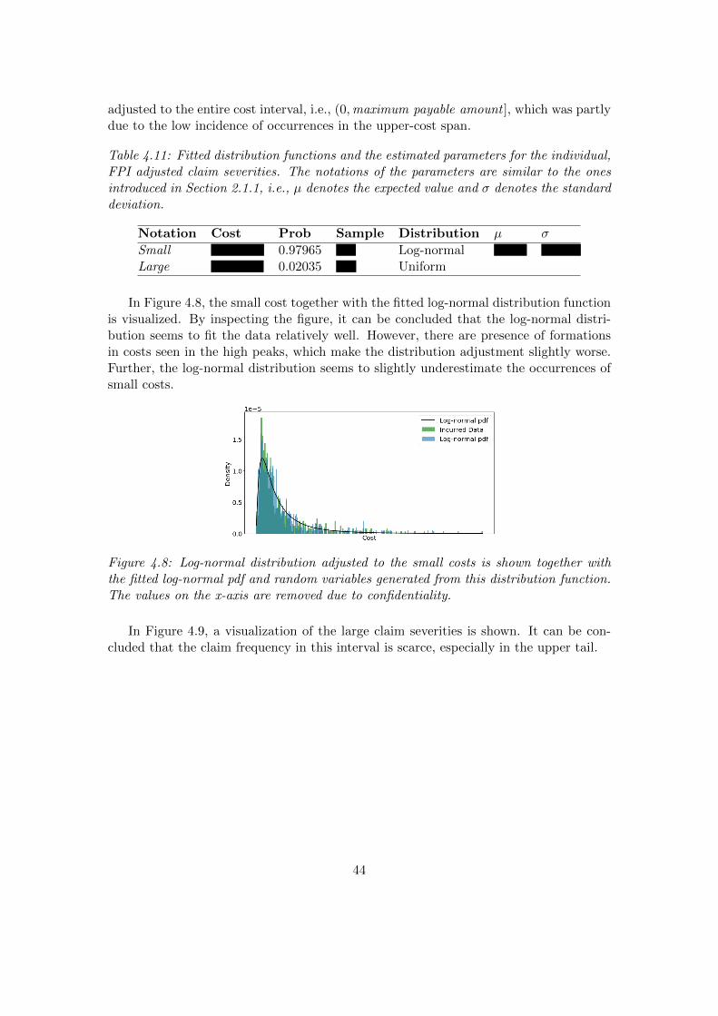
adjusted to the entire cost interval, i.e., (0,maximum payable amount ], which was partlydue to the low incidence of occurrences in the upper-cost span.

Table 4.11: Fitted distribution functions and the estimated parameters for the individual,FPI adjusted claim severities. The notations of the parameters are similar to the onesintroduced in Section 2.1.1, i.e., µ denotes the expected value and σ denotes the standarddeviation.

Notation Cost Prob Sample Distribution µ σ

Small 0.97965 Log-normalLarge 0.02035 Uniform

In Figure 4.8, the small cost together with the fitted log-normal distribution functionis visualized. By inspecting the figure, it can be concluded that the log-normal distri-bution seems to fit the data relatively well. However, there are presence of formationsin costs seen in the high peaks, which make the distribution adjustment slightly worse.Further, the log-normal distribution seems to slightly underestimate the occurrences ofsmall costs.

Figure 4.8: Log-normal distribution adjusted to the small costs is shown together withthe fitted log-normal pdf and random variables generated from this distribution function.The values on the x-axis are removed due to confidentiality.

In Figure 4.9, a visualization of the large claim severities is shown. It can be con-cluded that the claim frequency in this interval is scarce, especially in the upper tail.

44

Figure 4.9: The costs denoted as large. To those costs, a uniform distribution is fitted,but is not shown in the figure. The values on the x-axis are removed due to confidentiality.

4.5 Total Cost Distribution

In this section, the total cost distribution resulting from the number of claims fromPerspective 1, 2 and 3 are presented for each of the products separately.

4.5.1 Perspective 1

In this section, the total cost for contracts related to underwriting year 2021 is presented.The total cost distribution is evaluated based on the two approaches: parametric andhistoric, and based on the three methods: Single Risk, Bootstrap and Scenario.

Product A

In Table 4.12, the estimated total cost for contracts with underwriting year 2021 ispresented for the parametric and historic approach and all three risk methods. By in-specting the table, it can be concluded that the historic approach results in a smaller costspan than the parametric approach, when compared for the same method. Further, themethod Single Risk results in a larger reserve than the Bootstrap method, if comparedagainst the 50th percentile, but have a lower standard deviation. The result stands forboth approaches and can be further strengthened by inspecting Table 4.13.

45

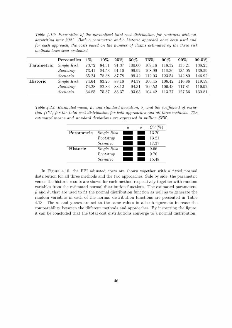
Table 4.12: Percentiles of the normalized total cost distribution for contracts with un-derwriting year 2021. Both a parametric and a historic approach have been used and,for each approach, the costs based on the number of claims estimated by the three riskmethods have been evaluated.

Percentiles 1% 10% 25% 50% 75% 90% 99% 99.5%

Parametric Single Risk 73.72 84.31 91.37 100.00 109.16 118.32 135.21 138.25Bootstrap 73.41 84.53 91.10 99.92 108.99 118.36 135.05 139.59Scenario 65.24 78.38 87.78 99.42 112.03 123.54 142.80 146.92

Historic Single Risk 74.64 83.25 88.18 94.37 100.45 106.42 116.86 119.59Bootstrap 74.28 82.83 88.12 94.31 100.52 106.43 117.81 119.92Scenario 64.85 75.37 83.37 93.65 104.42 113.77 127.56 130.81

Table 4.13: Estimated mean, µ, and standard deviation, σ, and the coefficient of varia-tion (CV) for the total cost distribution for both approaches and all three methods. Theestimated means and standard deviations are expressed in million SEK.

µ σ CV (%)

Parametric Single Risk 13.20Bootstrap 13.21Scenario 17.37

Historic Single Risk 9.66Bootstrap 9.76Scenario 15.48

In Figure 4.10, the FPI adjusted costs are shown together with a fitted normaldistribution for all three methods and the two approaches. Side by side, the parametricversus the historic results are shown for each method respectively together with randomvariables from the estimated normal distribution functions. The estimated parameters,µ and σ, that are used to fit the normal distribution function as well as to generate therandom variables in each of the normal distribution functions are presented in Table4.13. The x- and y-axes are set to the same values in all sub-figures to increase thecomparability between the different methods and approaches. By inspecting the figure,it can be concluded that the total cost distributions converge to a normal distribution.

46

(a) Parametric Single Risk (b) Historic Single Risk

(c) Parametric Bootstrap (d) Historic Bootstrap

(e) Parametric Scenario (f) Historic Scenario

Figure 4.10: Estimated total cost distribution for contracts written in year 2021 togetherwith a fitted normal distribution function and generated random variables from the dis-tribution function. The estimated parameters, µ and σ, are presented in Table 4.13. Thevalues on the x-axes are removed due to confidentiality.

Product B

In Table 4.14, the estimated total cost for contracts with underwriting year 2021 ispresented for both approaches and the three risk methods. By inspecting the table, it canbe concluded that both the parametric and the historic approach result in approximatelythe same total cost, independently of the method applied. Although, it should be pointedout that the parametric approach results in a slightly higher cost in the upper percentiles,than the historic approach does. Further, the Scenario method results in a moderately

47

wider cost span than the other two methods.

Table 4.14: Percentiles of the normalized total cost distribution for contracts with under-writing year 2021. Both a parametric and a historic approach have been used and, foreach approach, the costs based on the number of claims estimated by the three risk meth-ods have been evaluated. The results are normalized with respect to the 50th percentileof the parametric, Single Risk method.

Percentiles 1% 10% 25% 50% 75% 90% 99% 99.5%

Parametric Single Risk 64.26 78.01 88.19 100.00 113.49 126.72 149.93 157.10Bootstrap 62.82 77.73 87.78 99.81 113.48 126.38 151.20 155.05Scenario 57.03 73.05 85.30 100.29 116.72 132.16 161.40 168.49

Historic Single Risk 64.37 78.50 87.78 99.20 111.35 123.73 144.67 149.73Bootstrap 63.79 78.16 87.73 98.86 111.38 123.71 145.44 149.27Scenario 56.14 73.60 84.51 98.24 113.64 129.39 157.85 162.77

The estimated means, standard deviations and coefficients of variation of the totalcost distributions are presented in Table 4.15.

Table 4.15: Estimated mean, µ, and standard deviation, σ, and the coefficient of varia-tion (CV) for the total cost distribution for both approaches and all three methods. Theestimated means and standard deviations are expressed in million SEK.

µ σ CV (%)

Parametric Single Risk 18.59Bootstrap 18.89Scenario 22.69

Historic Single Risk 17.45Bootstrap 17.74Scenario 21.81

In Figure 4.11, the FPI adjusted costs are shown together with a fitted normaldistribution for all three methods and the two approaches. Side by side, the parametricversus the historic results are shown for each method respectively together with randomvariables from the estimated normal distribution functions. The estimated parameters,µ and σ, that are used to fit the normal distribution function as well as to generate therandom variables in each of the normal distribution functions are presented in Table4.15. The x- and y-axes are set to the same values in all sub-figures to increase thecomparability between the different methods and approaches.

48

(a) Parametric Single Risk (b) Historic Single Risk

(c) Parametric Bootstrap (d) Historic Bootstrap

(e) Parametric Scenario (f) Historic Scenario

Figure 4.11: Estimated total cost distribution for contracts written in year 2021 togetherwith a fitted normal distribution function and generated random variables from this dis-tribution function. The estimated parameters, µ and σ, are presented in Table 4.15. Thevalues on the x-axes are removed due to confidentiality.

4.5.2 Perspective 2

In this section, the estimated total cost for accident year 2021, for already active con-tracts and for contracts with underwriting year 2021, is presented. Both a parametricand a historic approach reflecting the individual claim severities are used in combinationwith the three risk methods.

49

Product A

In Table 4.16, the estimated total cost for accident year 2021 is presented for the para-metric and historic approach. For both approaches, the three risk methods are applied.

By inspecting Table 4.16, it can be concluded that the parametric approach resultsin a larger reserve in the 50th percentile than the historic approach does, independentlyof risk method used. Further, if the same risk method is compared between the twoapproaches it can be concluded that the parametric approach results in a wider spreadin the estimated total cost. The result applies to all three methods.

Table 4.16: Percentiles of the normalized total cost distribution for accident year 2021.Both a parametric and a historic approach have been used and, for each approach, thecosts based on the number of claims estimated by the three risk methods have been eval-uated. The results are normalized to the 50th percentile with the parametric, Single Riskmethod.

Percentiles 1% 10% 25% 50% 75% 90% 99% 99.5%

Parametric Single Risk 73.86 84.83 91.84 100.00 109.92 118.71 135.40 139.46Bootstrap 73.71 84.57 91.59 100.26 109.80 119.20 136.18 142.00Scenario 70.62 82.05 89.97 99.96 111.31 121.25 139.44 145.36

Historic Single Risk 73.48 82.82 88.18 94.36 100.82 106.75 117.48 120.90Bootstrap 74.78 83.11 88.37 94.39 101.06 106.97 117.80 121.12Scenario 70.04 80.38 86.51 94.41 102.38 109.72 122.35 125.78

The estimated means, standard deviations and coefficients variation for the total costdistributions are presented in Table 4.17.

Table 4.17: Estimated mean, µ, and standard deviation, σ, and the coefficient of vari-ation of the total cost distribution for both approaches and all three methods. The esti-mated means and standard deviations are expressed in million SEK.

µ σ CV (%)

Parametric Single Risk 13.09Bootstrap 13.47Scenario 15.18

Historic Single Risk 9.91Bootstrap 9.86Scenario 12.09

In Figure 4.12, the FPI adjusted costs are shown together with a fitted normaldistribution for all three methods and the two approaches. Side by side, the parametricversus the historic results are shown for each method respectively, together with randomvariables from the estimated normal distribution functions. The estimated parameters,µ and σ, that are used to fit the normal distribution function as well as to generate therandom variables in each of the normal distribution functions are presented in Table

50

4.17. The x- and y-axes are set to the same values in all sub-figures to increase thecomparability between the different methods and approaches.

(a) Parametric Single Risk (b) Historic Single Risk

(c) Parametric Bootstrap (d) Historic Bootstrap

(e) Parametric Scenario (f) Historic Scenario

Figure 4.12: Estimated total cost distribution for all active contracts and for accidentyear 2021. The estimated values are shown together with a fitted normal distributionfunction and generated random variables from this distribution function. The estimatedparameters, µ and σ, are presented in Table 4.17. The values on the x-axes are removeddue to confidentiality.

Product B

In Table 4.18, the estimated total cost for accident year 2021 is presented for both theparametric and the historic approach. For both approaches, all three risk methods, i.e.

51

Single Risk, Bootstrap and Scenario, are applied.By inspecting Table 4.18, it can be concluded that the parametric approach and the

historic approach result in approximately the same total cost for the 50th percentile.However, if the same risk method is compared between the two approaches, it can beconcluded that the parametric approach results in a slightly wider cost spread. Theresult applies to all three risk methods.

Table 4.18: Percentiles of the normalized total cost distribution for accident year 2021.Both a parametric and a historic approach have been used and, for each approach, thecosts based on the number of claims estimated by the three risk methods have been eval-uated. The results are normalized to the 50th percentile in relation to the parametric,Single Risk method.

Percentiles 1% 10% 25% 50% 75% 90% 99% 99.5%

Parametric Single Risk 63.29 77.86 87.89 100.00 113.77 126.22 150.38 158.80Bootstrap 62.40 76.55 86.65 99.15 112.29 125.51 151.39 158.43Scenario 58.61 74.92 85.88 99.48 113.90 127.38 154.45 160.13

Historic Single Risk 64.95 78.49 87.94 98.96 111.36 123.24 146.56 151.42Bootstrap 62.22 76.78 86.71 97.98 110.44 122.09 143.56 149.60Scenario 60.23 75.55 86.13 98.71 112.15 125.60 148.76 154.83

The estimated means, standard deviations and coefficients of variations for the totalcost distributions are presented in Table 4.19.

Table 4.19: Estimated mean, µ, and standard deviation, σ, and the coefficient of varia-tion (CV) for the total cost distribution for both approaches and all three methods. Theestimated means and standard deviations are expressed in million SEK.

µ σ CV (%)

Parametric Single Risk 18.90Bootstrap 19.37Scenario 20.70

Historic Single Risk 17.55Bootstrap 17.86Scenario 19.38

The FPI adjusted costs are shown in Figure 4.13 together with a fitted normal dis-tribution for all three methods and both of the two approaches. Side by side, the resultsfor the parametric versus the historic approach are shown for each method respectivelytogether with random variables from the estimated normal distribution functions. Theestimated parameters, µ and σ, used to fit the normal distribution function as well asto generate the random variables in each normal distribution function are presented inTable 4.19. The x- and y-axes are set to the same values in all sub-figures to increasethe comparability between the different methods and approaches.

52

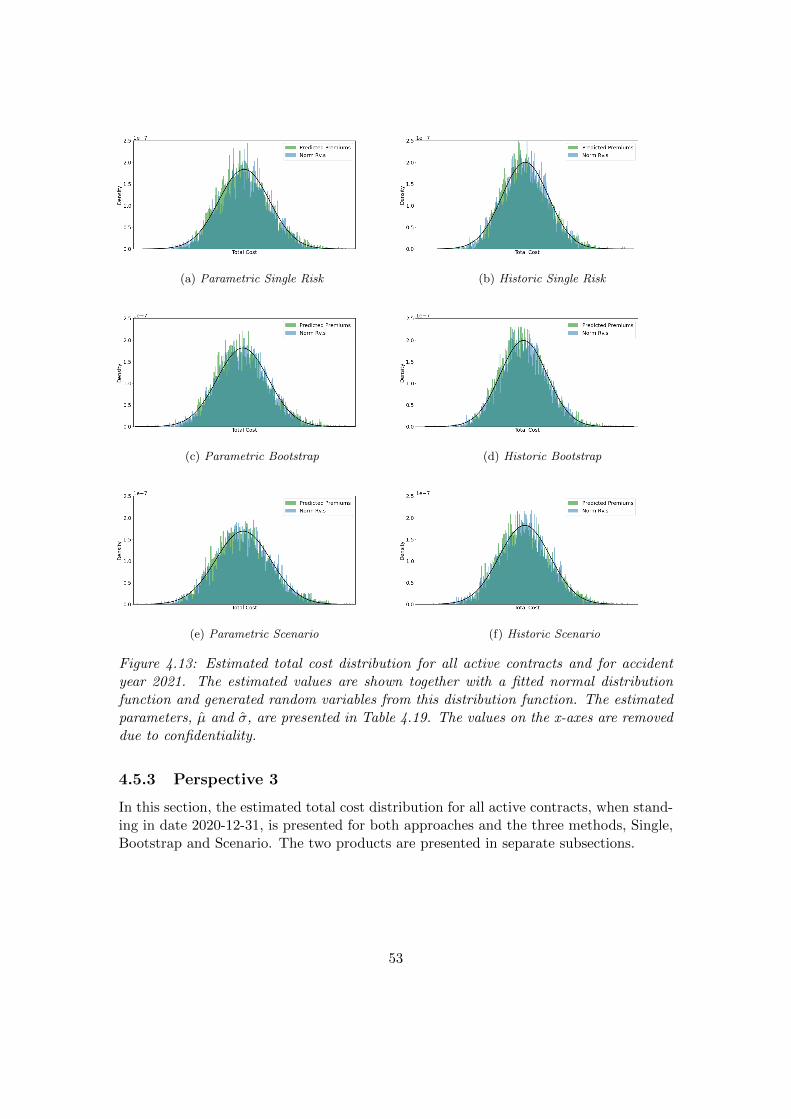
(a) Parametric Single Risk (b) Historic Single Risk

(c) Parametric Bootstrap (d) Historic Bootstrap

(e) Parametric Scenario (f) Historic Scenario

Figure 4.13: Estimated total cost distribution for all active contracts and for accidentyear 2021. The estimated values are shown together with a fitted normal distributionfunction and generated random variables from this distribution function. The estimatedparameters, µ and σ, are presented in Table 4.19. The values on the x-axes are removeddue to confidentiality.

4.5.3 Perspective 3

In this section, the estimated total cost distribution for all active contracts, when stand-ing in date 2020-12-31, is presented for both approaches and the three methods, Single,Bootstrap and Scenario. The two products are presented in separate subsections.

53

Product A

The estimated total cost is presented in Table 4.20. In the table, a number of percentilesshowing the total cost from both approaches and all three methods are presented. Itcan be concluded that the spread of the total cost increases as the methods proceedfrom Single to Bootstrap and lastly to Scenario. The estimated total cost in the 50thpercentile is relatively similar between the methods and the approaches, but it should bepointed out that the parametric approach results in a slightly higher best estimate, i.e.50th percentile, as well as a wider cost interval. This result is applicable to all methods.

Table 4.20: Percentiles of the normalized total cost distribution for all active contracts,when standing in 2020-12-31. Both a parametric and a historic approach have been usedand, for each approach, the costs based on the number of claims estimated by the threerisk methods have been evaluated. The results are normalized with respect to the 50thpercentile of the parametric, Single Risk method.

Percentiles 1% 10% 25% 50% 75% 90% 99% 99.5%

Parametric Single Risk 79.44 87.96 93.46 100.00 107.17 114.11 125.81 129.19Bootstrap 77.32 87.02 92.99 100.26 107.77 114.87 129.59 133.74Scenario 68.55 80.56 89.27 100.44 111.96 122.02 140.99 144.66

Historic Single Risk 78.85 85.54 89.57 94.18 99.18 103.58 112.08 113.77Bootstrap 76.82 84.00 88.78 94.40 99.96 104.95 114.65 116.84Scenario 66.55 76.96 84.49 94.40 104.12 112.16 125.40 128.19

In Table 4.21, the estimated means, standard deviations and coefficients of variationof the fitted normal distribution functions to the total costs are presented. It can beconcluded that the standard deviation is larger for the parametric approach than it isfor the historic approach, if the same method is compared. Further, it can be concludedthat the standard deviation of the estimated total cost distributions increases as themethod goes from Single to Bootstrap to Scenario.

Table 4.21: Estimated mean, µ, and standard deviation, σ, and the coefficient of varia-tion (CV) for the total cost distribution for both approaches and the three methods. Theestimated means and standard deviations are expressed in million SEK.

µ σ CV (%)

Parametric Single Risk 10.11Bootstrap 11.00Scenario 15.82

Historic Single Risk 7.49Bootstrap 8.58Scenario 14.19

In Figure 4.14, the total costs are visualized together with fitted probability den-sity functions for the normal distribution and with random variables generated from

54

those normal distributions. The estimated parameters, µ and σ, are presented in Table4.21. The x- and y-axes are set to the same values in all sub-figures to increase thecomparability between the different methods and approaches.

(a) Parametric Single Risk (b) Historic Single Risk

(c) Parametric Bootstrap (d) Historic Bootstrap

(e) Parametric Scenario (f) Historic Scenario

Figure 4.14: Estimated total cost distribution for all active contracts, when standingin 2020-12-31, together with a fitted normal distribution function and generated ran-dom variables from this distribution function. The estimated parameters, µ and σ, arepresented in Table 4.21. The values on the x-axes are removed due to confidentiality.

Product B

In Table 4.22, the estimated total cost for all active contracts is presented for the para-metric and the historic approach and all three methods. By inspecting the table, it can

55

be concluded that the spread of the total cost gets larger as the method goes from Singleto Bootstrap to Scenario. Further, it can be noted that the parametric approach resultsin a larger total cost than the historic approach, especially if compared in the upperpercentiles and between the same method.

Table 4.22: Percentiles of the normalized total cost distribution for all active contracts,when standing in 2020-12-31. Both a parametric and a historic approach have been usedand, for each approach, the costs based on the number of claims estimated by the threerisk methods have been evaluated. The results are normalized with respect to the 50thpercentile of the parametric, Single Risk method.

Percentiles 1% 10% 25% 50% 75% 90% 99% 99.5%

Parametric Single Risk 70.00 81.60 89.97 100.00 110.69 120.97 141.45 146.61Bootstrap 65.38 79.23 89.19 100.69 112.66 125.13 147.08 153.27Scenario 58.22 75.25 86.06 100.29 115.40 129.74 154.77 164.68

Historic Single Risk 69.48 81.72 89.23 98.37 108.49 118.46 136.35 140.56Bootstrap 65.28 79.67 88.79 99.66 111.34 121.73 140.20 145.12Scenario 59.34 74.65 85.45 99.45 113.57 127.05 153.94 159.44

In Table 4.23, the estimated means, standard deviations and coefficients of variationof the fitted normal distribution functions are presented. It can be concluded that themean is relatively similar for both approaches and that the estimated standard deviationincreases as the method proceed from Single Risk to Bootstrap to Scenario.

Table 4.23: Estimated mean, µ, and standard deviation, σ, and the coefficient of varia-tion (CV) for the total cost distribution for both approaches and all three methods. Theestimated means and standard deviations are expressed in million SEK.

µ σ CV (%)

Parametric Single Risk 15.37Bootstrap 17.49Scenario 21.04

Historic Single Risk 14.41Bootstrap 16.45Scenario 20.36

In Figure 4.15, the total costs are visualized together with fitted probability den-sity functions for the normal distribution and with random variables generated fromthose normal distributions. The estimated parameters, µ and σ, are presented in Table4.23. The x- and y-axes are set to the same values in all sub-figures to increase thecomparability between the different methods and approaches.

56

(a) Parametric Single Risk (b) Historic Single Risk

(c) Parametric Bootstrap (d) Historic Bootstrap

(e) Parametric Scenario (f) Historic Scenario

Figure 4.15: Estimated total cost distribution for all active contracts, when standingin 2020-12-31, together with a fitted normal distribution function and generated ran-dom variables from the distribution function. The estimated parameters, µ and σ, arepresented in Table 4.23. The values on the x-axes are removed due to confidentiality.

57

5. Discussion and Conclusions

In this chapter, general comments of the results are presented and discussed. Areas in-cluded in the discussions are the Poisson assumption, the claim frequencies, and the costof claims. Further, the result of the total cost distributions are compared and discussedand lastly, final conclusions regarding which models that are most accurate are made.

5.1 General Comments

5.1.1 Poisson Assumption

The Poisson assumption was at neither of the tested significance levels rejected forProduct A, but was rejected on a 95% confidence level for Product B. Despite therejection of the null hypothesis for Product B, the Poisson distribution was applied todescribe the claim counts for both products. The tested data for Product B indicated atoo high observed frequency for the lowest number of claims, compared to the expectedPoisson frequency. Therefore, the Poisson distribution would indicate slightly too manyclaims, compared to what the historic data indicated.

Based on the similarities of the two products, the underlying process that describesthe number of claims is assumed to be similar to each other. Further, both productshave a limited amount of claims data and depending on how the time splits were made,the resulting test statistics differed a lot, especially for Product B. This is caused bythe lack of data in the periods, which makes it highly sensitive to the groupings. Withthis in mind, the results from the tests were not definite in the decision of underlyingdistributions and more concern was weighted towards the actuarial team’s knowledgeand recommendations about the products.

5.1.2 Claim Frequency

The three perspectives of which the claim frequency has been evaluated against, resultedin different outcomes, which is expected due to the differences in number of contractsand time horizons. However, the result from Perspective 1 as well as the result fromPerspective 2 distinguish in a way that was not expected: the Single Risk method resultsin approximately equally many claims, and sometimes more, than the Bootstrap methoddoes, for both products. At first glance, this was not anticipated since the Bootstrapmethod incorporates more uncertainty than the Single Risk method. However, the result

58

is explained by the same argument. The uncertainty is larger in the later period of thecontract for the Bootstrap method, which can be seen in Figure 4.2 and Figure 4.3 ifthey are compared between each other. This leads to approximately the same estimateof the number of claims in the first part of the period, but if the entire contract periodis considered, then the Bootstrap method results in more claims than the Single Riskmethod. The intended difference between Figure 4.2 and Figure 4.3 can be difficult todecipher, but if they are carefully studied it can be seen that the spread (in the verticaldirection) is relatively slim at the very beginning of the contract period in the Bootstrapmethod and thereafter gets wider. The higher located the curve is, the larger remaininguncertainty, i.e., the risk of the contract. A natural question then is why we do not seea similar result when the Scenario method is applied. Most likely, this can be explainedby the fact that the vertical offset in the risk curve makes an evident impact in theentire time period of the contract. To clarify, the Scenario can be interpreted as ”theuncertainty” of a claim during the lifetime of this contract is best estimate * [1 ± 0.2],i.e., somewhere in the interval [0.8 * best estimate, 1.2 * best estimate]. Since all theoutcomes in the offset are equally probable and the magnitude of the offset is identicalin both directions, the 50th percentile is expected to be the same as the result from theSingle Risk and the Bootstrap method. However, the uncertainty will further result infewer claims in the percentiles below fifty, and more claims in the percentiles above fifty,which is thereto verified in the results.

5.1.3 Cost of Claims

Two approaches have been applied to estimate the cost of a claim: a parametric and ahistoric approach. A few pros and cons of those two have been discussed in Section 3.2.6,but can again be noted. The parametric approach has the obvious disadvantage thatif the distribution is not a good approximation of the true distribution, then applyingthe distribution will result in an incorrect result that should not be trusted. However,if the distribution is a good approximation of the underlying process, the result can bevery satisfactory. The historic approach on the other hand, will always be wrong, buthopefully not too wrong. To clarify, assuming that future costs never can differ fromhistorically observed costs is probably not a supportable assumption. The inadequacygets most evident in the extreme cost interval, where the number of data points is few.It is difficult to argue why we in the future only expect the very few outcomes that wehave had in the past, and no others. This is a palpable disadvantage with the historicapproach and is also the reason to why the historic approach results in lower predictedcosts, than the parametric approach does.

As discussed in the theory section, accretion of costs is common in insurance data.This aggravates the process of adjusting a distribution to the data. If those accretionsof costs are modeled, then the model will become too complicated and if they are partlyignored, then the fit of the model can appear worse than it is. This, together withthe fact that we deal with large samples, complicate the statistical verification of thedistributions’ fit to the data. Therefore, to verify if the parametric adjustments are goodapproximations of the true cost distributions, visualizations of the data together with

59

the fitted distributions and random variables generated from those, have composed asthe test base.

Further, the presence of data is not equal in the entire indemnity interval. In theupper part of the interval, uniform distributions have been assumed. When inspectingFigure 4.7 and Figure 4.9, it looks like the risk of getting a claim in the lower part of theinterval is higher than in the upper part. Although, based on the low frequency of datapoints in the interval, a more complex distribution would probably be too volatile andshould therefore not be trusted. As an example, assume that some sort of highly right-skewed distribution was fitted to the interval for both products. If the insurance companythen would have as few as five claims or two claims in the upper part of the interval, thedistribution would change from a highly right-skewed distribution to a highly left-skeweddistribution, for the two products respectively. If such few data points completely couldchange the entire shape of the distribution, then we find if hard to motivate that thosedifferences should be modeled. Instead, a more reasonable assumption is to assume equalprobability, until more data is available.

5.1.4 Total Cost Distribution

By inspecting the results, it can be concluded that the parametric approach, in general,results in a higher reserve than the historic approach does, even though the differencesin the 50th percentiles are slim. The fact that the best estimate, i.e., the 50th percentile,is very alike between the two approaches makes us feel assuaged of the adjusted distri-butions. This tells us that the best estimate of the reserve, in median terms spoken,does not depend much on the chosen approach. However, due to the evident drawbackof the historic approach and the relatively satisfactory fit in the parametric approach,we strongly believe that the parametric approach engages the true variation and thetrue best estimate of the total cost distributions better. With this stated, this doesnot mean that the actual variation of the true total cost distribution is captured by theparametric approach, even though we do feel satisfied with the adjusted distributionsto the costs’ data. It should however be remembered that the total cost distributionsare highly affected by the probabilities of choosing each respective distribution. Theseprobabilities are estimated from the FPI adjusted historic data, and do not necessarilyhave to be representative in the future. On the other hand, in Figure 3.3 and Figure 3.6,the historical claim severities are shown and it can be seen that they have not increasedover time. Important to note is that the costs in those figures are not FPI adjusted.Therefore, if the FPI adjustment is taken into account, the average claim severity hasdecreased over time. According to the actuarial team, this depends on an increasedwork standard performed by the inspection technicians. The result is that the increasedstandard has netted out the effect of increased building costs. Since this effect is not as-sumed to continue in the future, the estimated probabilities and distributions are basedon FPI adjusted claim severities and with this stated, by using these distributions andprobabilities, we rather tend to overestimate the costs than the opposite.

Another perspective that is important to evaluate is which one of the risk methodswe consider predict the future best. Since the insurance product has a horizon of 10

60

years, time is a natural uncertainty factor. Many aspects highlight the importanceto know the expected cost: the pricing of the insurance products, the evaluation ofreinsurance contracts and last but not least, the reserve amount needed to stay solvent.With this stated, we do not feel confident to say that the future will not differ comparedto the past and therefore, both the Single Risk- and the Bootstrap method have obviousshortcomings. However, the Scenario risk curve incorporates both indications from thepast and takes into account reasonable changes that lie in the future. If we only considerthe parametric - Scenario results, a reasonable question to ask is if we do feel confidentwith the adjusted distributions. In accordance with the central limit theorem, the totalcost distributions converge to a normal distribution. The question is, do we feel confidentthat the estimated standard deviation, σ, is a sensible estimate of the true standarddeviation, σ. Without possessing the expert knowledge about the products, it is difficultto judge whether the estimate, σ, is sensible or not. Therefore, the actuarial team’ssense has been highly valued and has acted as an important element in the evaluationof the estimates. With this stated, we do believe that the estimated standard deviationscapture the true standard deviation for Perspective 1 and 3. For Perspective 2 however,we believe that a scenario which incorporates a variation of ± 20% overestimates the riskand that another, lower scenario, not included in this thesis, can be a better estimate.

5.2 Conclusions

To conclude, the Scenario risk curves capture the future best of the applied methods. Theestimated standard deviations of the total cost distributions for Perspective 1 and 3 aresensible. However, the estimated standard deviation of the total cost for Perspective 2 isbelieved to be too high, due to the applied scenario. Remark that the estimated numberof claims and the estimated costs for Perspective 2 have a time horizon of one year,in contrast to Perspective 1 and 3, which have a time horizon of ten years. Therefore,the Bootstrap method is considered as the most accurate prediction, among the appliedmethods, of the risk for Perspective 2.

The parametric approach is considered the most reliable, since it does not only coveroutcomes seen in the past. In the small cost intervals, relatively much data are availableand we feel confident with the adjusted distributions. The same holds for the largecost distribution for Product A. In the highest cost interval, i.e., extreme for ProductA and large for Product B, we recommend that the uniform distribution assumption ischallenged as soon as a sufficient amount of data is available.

To summarize, the estimated parameters of the total cost distributions that areconsidered the most accurate in each respective perspective are presented in Table 5.1.

5.2.1 Final Models

In Perspective 1 and 3, the parametric approach applied with the Scenario method isconsidered the most reliable. In Perspective 2, the parametric approach applied withthe Bootstrap method is considered the most reliable.

61

Table 5.1: Summary of the estimated parameters of the best models. Perspective 1 and 3correspond to the risk method Scenario and Perspective 2 corresponds to the risk methodBootstrap. In all three perspectives, the parametric approach is used to estimated thecosts.

Perspective 1 Perspective 2 Perspective 3

Product A Product B Product A Product B Product A Product Bµσ

5.3 Recommendations

Due to the time constraint of this thesis, some delimitations had to be made and areaswhich we wanted to investigate more thoroughly had to be given a lower priority. Tofuture studies, we therefore recommend the following areas to be investigated further

• Challenge the distribution assumption of the number of claims by applying, e.g.,a negative binomial distribution.

• Challenge the distribution assumptions of the claim severities.

• Challenge the time-assumption reflecting the size of a claim, i.e., if the probabilityof a large claim severity is greater in the beginning of the contract’s lifetime.

• Challenge the risk curve calculations by putting, e.g., a large weight to more recentunderwriting years.

• Investigate if a model that describes when the predicted claims will be reportedcan be found. The model can then be used to predict when claims will occurand not only if/if not a claim will occur. To clarify: by applying the risk curvesin accordance with the approach suggested in this thesis, the obtained estimateshows how many claims that are expected during a determined period and notwhen in this period they occur.

• Develop a more complex model which describes the number of contracts that areexpected to be written during a certain period.

62

References

Anticimex. 2019. Annual report.https://www.anticimex.com/globalassets/_sverige-sv-se/forsakringsbolaget/

media/arsredovisning-2019.pdf. (Retrieved: 2021-02-04).

Anticimex. n.d. Saljaransvarsforsakring - skydda dig mot dolda fel.https://www.anticimex.com/sv-se/privatkunder/vara-tjanster/saljaransvarsforsakring/.(Retrieved: 2021-05-04).

Anticimex. 2018. Vad ar ett dolt fel?. https://www.anticimex.com/sv-se/nyhetsrum/2017/vad-ar-ett-dolt-fel/. (Retrieved: 2021-05-04).

Aviva. 2021. How we´re organised.https://www.aviva.com/about-us/how-we-are-organised/. (Retrieved: 2021-05-12).

Bjorkwall, Susanna. 2011. Stochastic claims reserving in non-life insurance. Stock-holms Universitet. ISBN 978-91-7447-255-4.

International Actuarial Association. 2013. THE ROLE OF THE ACTUARY.http://www.actuaries.org/LIBRARY/Papers/role_actuary_en.pdf. (Retrived: 2021-05-12).

Johansson, Bjorn. 2014. Matematiska modeller inom sakforsakring. [Kompendium].Stockholms Universitet. Matematiska Institutionen. Matematisk Statistik.

Mack, Thomas. 1993. Measuring the variability of chain ladder reserve estimates.https://www.casact.org/pubs/forum/94spforum/94spf101.pdf. (Retrieved: 2020-02-25).

Martınez Mirande, Marıa Dolores; Nielsen, Jens Perch; Verrall, Richard. n.d.. Dou-ble Chain Ladder.https://www.actuaries.org/ASTIN/Colloquia/Madrid/Papers/Miranda_Nielsen_Verrall_

1.pdf. (Retrieved: 2021-02-25).

Ohlsson, Esbjorn. 2017. Skadeforsakringsredovisning for aktuarier. [Kompendium].Stockholms Universitet. Matematiska Institutionen. Matematisk Statistik.

SCB. 2021. Faktorprisindex for byggnader (FPI).https://www.scb.se/vara-tjanster/scbs-olika-index/bygg--och-fastighetspriser/

faktorprisindex-for-byggnader-fpi/. (Retrieved: 2021-04-20).

Renshaw, Artur; Verrall, Richard. 1998. A stochastic model underlying the chain-ladder

63

technique.https://doi.org/10.1017/S1357321700000222. (Retrieved: 2021-02-25).

Scipy. n.d. Scientific computing tools for Python. https://www.scipy.org/about.

html. (Retrieved: 2021-05-04).

SFS 1970:994. Jordabalk

Taleb, N. 2020. Statistical Consequences of Fat Tails: Real World Preasymtotics, Epis-temology, and Applications (The Technical Incerto Collection). STEM Academic Press.

U.S. Bureau of Labor Statistics. 2021. Actuaries.https://www.bls.gov/ooh/math/actuaries.htm?view_full. (Retrieved: 2021-05-12).

Wolfram Research. 2016. Gamma Distribution, Wolfram Language function. https://

reference.wolfram.com/language/ref/GammaDistribution.html. (Retrieved: 2021-04-06).

64

Appendices

65

A. Product A

Claim Cost - Accident Month

Figure A.1: Box plot illustrating the claim costs based on the month of the accident. Thevalues on the y-axis are removed due to confidentiality.

66

Claim Cost - Accident Year

Figure A.2: Box plot illustrating the claim costs based on the year of the fault. Thevalues on the y-axis are removed due to confidentiality.

Claim Cost - Underwriting Month

Figure A.3: Box plot illustrating the claim costs depending on the contracts’ underwritingmonth. The values on the y-axis are removed due to confidentiality.

67

B. Product B

Claim Cost - Accident Month

Figure B.1: Box plot illustrating the claim costs based on the month of the accident. Thevalues on the y-axis are removed due to confidentiality.

68

Claim Cost - Accident Year

Figure B.2: Box plot illustrating the claim costs based on the year of the fault. Thevalues on the y-axis are removed due to confidentiality.

Claim Cost - Underwriting Month

Figure B.3: Box plot illustrating the incurred claim cost depending on the contracts’underwriting month. The values on the y-axis are removed due to confidentiality.

69

Percentage Number of Contracts

(a) Underwriting Year 2013 (b) Underwriting Year 2014

(c) Underwriting Year 2015 (d) Underwriting Year 2016

(e) Underwriting Year 2017 (f) Underwriting Year 2018

(g) Underwriting Year 2019

Figure B.4: The percentage number of contracts written in each month during the un-derwriting years 2013-2019.

70