evaluation of the sedov-von neumann-taylor blast wave...

Evaluation of the Sedov-von Neumann-Taylor

Blast Wave Solution

James R. Kamm

Integrated Physics Group, MS D413Applied Physics Division

Los Alamos National LaboratoryLos Alamos, NM 87545 USA

December 21, 2000

LA-UR-00-6055

Contents

List of Figures vi

List of Tables vi

Abstract 1

1 Introduction 1

2 The Sedov Solution 12.1 Similarity Variables . . . . . . . . . . . . . . . . . . . . . . . . . . 22.2 Closed-form Solution . . . . . . . . . . . . . . . . . . . . . . . . . 32.3 The Energy Integral . . . . . . . . . . . . . . . . . . . . . . . . . 7

2.3.1 Standard or Vacuum Case . . . . . . . . . . . . . . . . . . 92.3.2 Singular Case . . . . . . . . . . . . . . . . . . . . . . . . . 11

3 Numerical Evaluation of the Sedov Solution 14

4 Results 154.1 Constant Initial Density Test Cases . . . . . . . . . . . . . . . . . 164.2 Variable Initial Density Test Cases . . . . . . . . . . . . . . . . . 204.3 Hydrocode Comparisons . . . . . . . . . . . . . . . . . . . . . . . 23

4.3.1 Uniform Density Problem Comparison . . . . . . . . . . . 234.3.2 Singular Problem Comparison . . . . . . . . . . . . . . . . 294.3.3 Vacuum Problem Comparison . . . . . . . . . . . . . . . . 33

5 Summary 37

Acknowledgments 38

References 39

A Spatial Convergence Analysis 41

v

List of Figures

1 Results of uniform density test cases. . . . . . . . . . . . . . . . . 212 Results of singular test cases. . . . . . . . . . . . . . . . . . . . . 223 Results of vacuum test cases. . . . . . . . . . . . . . . . . . . . . 244 Results of RAGE on the uniform density test case, 120 zones. . . 265 Results of RAGE on the uniform density test case, 960 zones. . . 276 Results of RAGE on the singular test case, 120 zones. . . . . . . 307 Results of RAGE on the singular test case, 960 zones. . . . . . . 318 Results of RAGE on the vacuum test case, 120 zones. . . . . . . 349 Results of RAGE on the vacuum test case, 960 zones. . . . . . . 35

List of Tables

1 Comparison of γ = 1.4 planar similarity variables. . . . . . . . . 172 Comparison of γ = 1.4 cylindrical similarity variables. . . . . . . 183 Comparison of γ = 1.4 spherical similarity variables. . . . . . . . 194 Comparison of uniform density test case parameters. . . . . . . . 205 Comparison of singular test case parameters. . . . . . . . . . . . 236 Comparison of vacuum test case parameters. . . . . . . . . . . . 257 Uniform density Sedov problem RAGE spatial convergence rates 288 Sedov singular problem RAGE spatial convergence rates . . . . . 329 Sedov vacuum problem RAGE spatial convergence rates . . . . . 36

vi

Abstract

In this note we state the solution put forward by Sedov [18] for theproblem of self-similar, one-dimensional, compressible hydrodynamics inwhich a finite amount of energy is released at the origin at the initial time.We review the closed-form solution given by Sedov, provde an algorithmicprocedure by which this solution can be computed, and compare theseresults with hydrocode calculations.

1 Introduction

In this note we state the solution put forward by Sedov [18] for the problemof self-similar, one-dimensional, compressible hydrodynamics in which a finiteamount of energy is released at the origin at the initial time. This problem is col-loquially referred to by some combination of names of the three luminaries thatoriginally obtained the solution to this problem, viz., Sedov [18], Taylor [21], andvon Neumann [22]. Of these authors, Sedov provides the most general closed-form solution, which we herein review and compare with hydrocode solutions.

The intention of this note is to distill the thorough exposition given by Sedovinto a more compact and accessible form by providing the complete solution to-gether with the procedure by which to compute it. We present the full solutionin §2. The reader who desires only to calculate this solution is encouraged toproceed directly to §3, which contains the algorithmic procedure for evaluat-ing the solution. Section 4 contains examples of various solutions as well ascomparisons with hydrocode calculations. We close with a summary in §5.

In this report, we identify the corresponding equations of Chapter IV ofSedov’s book [18] as an equation number preceded by “S”; e.g., Eq. 1.3 ofChapter IV of [18] is denoted S1.3.

2 The Sedov Solution

In reference [18], Sedov considers the set of equations governing one-dimensional,compressible hydrodynamics. The set of evolution equations governing thisbehavior is given in physical space as (S1.3)

ρt + v ρr +ρ

rj−1

(rj−1 v

)r

= 0 , (1)

vt + v vr +1ρ

pr = 0 , (2)

(p/ργ)t + u (p/ργ)r = 0 , (3)

where ρ is the density, v is the velocity, and p is the pressure. The index j = 1,2, or 3 is the dimensionality index for one-dimensional planar, cylindrical, or

1

spherical geometry, respectively. Implicit in these equations is the assumptionof the polytropic gas equation of state, so that

(γ − 1) e = p/ρ , (4)

where γ is the constant adiabatic exponent (equal to the ratio of specific heats inthis case) and e is the specific internal energy. Additionally, and in distinctionto the analysis of Reinicke & Meyer-ter-Vehn [16], heat conduction is assumedto be negligible, so that purely hydrodynamic motion occurs.

The final assumption is that initial density distribution is given by (S14.1)

ρ0(r) = A r−ω , (5)

where A and ω are constants. When the value of ω is identically zero, theinitial density is uniform. Sedov (Ch. IV, §5) shows that the value of ω must beconstrained to keep the integral of the density (i.e., the mass) finite accordingto

ω < j . (6)

2.1 Similarity Variables

The nondimensionalization of the flow variables is given in S1.1. With therelations preceding S5.12 for the blast wave case, those expressions simplify tothe following form:

v =r

tV , ρ =

A

rωR , p =

A

rω−2 t2P , (7)

where V , R, and P are the fundamental similarity solution variables. It isa straightforward exercise to show that these quantities are related to othervariables according to the following relations (cf. the discussion after S14.4):

r

r2≡ λ , (8)

v

v2≡ f ≡ (j + 2 − ω) (γ + 1)

4λ V , (9)

ρ

ρ2≡ g ≡ γ − 1

γ + 1λ−ω R , (10)

p

p2≡ h ≡ (j + 2 − ω)2 (γ + 1)

8λ2−ω P , (11)

where the subscript 2 on a variable denotes its immediate post-shock value.In the uniform initial density case (ω = 0), the above relations reduce to theexpressions in S11.10. Additionally, the similarity variable Z is defined as (see§2.2 of Ch.4 of [18])

Z ≡ γ P/R . (12)

2

An infinitely strong shock is assumed, so that the pre-shock pressure isnegligible, i.e., p1 → 0. This assumption is equivalent to a1/U → 0, where a1

is the pre-shock sound speed and U is the shock speed. With this assumptionsubstituted into the standard shock jump relations [23], the immediate post-shock state is determined as:

v2 =2

γ + 1U , ρ2 =

γ + 1γ − 1

ρ1 , p2 =2

γ + 1ρ1 U2 , (13)

where ρ1 is the immediate pre-shock density.From dimensional analysis, the shock position r = r2 is related to the total

energy E0 according to the similarity relation (cf. S5.2, S11.3, S14.4)

r2 = λ2

( E0

Aα

)1/(j+2−ω)

t2/(j+2−ω) . (14)

The constant α will be shown (Eq. 66) to be related to the nondimensionalenergy of the solution. From the above expression, the time t can be written

t = r(j+2−ω)/22 λ

−(j+2−ω)/22

( E0

Aα

)−1/2

. (15)

Also from Eq. 14, the shock speed U ≡ dr2/dt can be expressed as (S14.4)

dr2

dt=

2j + 2 − ω

r2

t=

2j + 2 − ω

r−(j−ω)/22 λ

(j+2−ω)/22

( E0

Aα

)1/2

. (16)

2.2 Closed-form Solution

Sedov provides the solution for the constant density initial condition (ω = 0)in all geometries (j = 1,2,3), and for the power law initial density (Eq. 5) inspherical geometry (j = 3). Here, we give expressions for the power law initialdensity valid in in all geometries.

Sedov shows that the unique solution curve passing through the shock pointmust satisfy the following relation (S14.6)

Z =γ − 1

2

V 2(V − 2

j+2−ω

)2

(j+2−ω) γ − V. (17)

There are three possible forms for the solution, all of which satisfy this equation.The correct solution form depends on the relation between the shock state anda singular point of the equations that occurs along the curve given in Eq. 17.

In terms of the similarity variables introduced in the previous section, theshock position r2 and immediate post-shock state V2 (S14.5) are given as

r = r2 ⇔ λ = λ2 = 1 ⇔ V = V2 =4

(j + 2 − ω) (γ + 1)

3

and Z = Z2 =8 γ (γ − 1)

(j + 2 − ω)2 (γ + 1)2. (18)

There is a singular point of the equations located at (S5.14)

V = V ∗ =2

(γ − 1) j + 2, (19)

Z = Z∗ =2 γ (γ − 1) [(2 − γ) j − ω]

[(γ − 1) j + 2]2 [(ω − 2) γ − j + 2]. (20)

For physical solutions that intersect this singular point, it must be true thatZ∗ ≥ 0; in this case, it is straightforward to show that ω must satisfy thefollowing constraint (S5.15):

2γ + j − 2γ

≥ ω ≥ (2 − γ) j , (21)

with equality if and only if Z∗ = 0.The relation between location of the shock point V2 and the singular point

V ∗ determines the nature of the solution as follows.

1. V2 < V ∗: Standard . In this case, a nonzero solution extends from theshock to the origin, at which the pressure is finite. The constraint on theintial density coefficient ω for this case is

ω <j(3 − γ) + 2(γ − 1)

γ + 1. (22)

The location of the origin corresponds to the values

r = 0 ⇔ λ = λ0 = 0 ⇔ V = V0 =2

(j + 2 − ω) γ. (23)

As the origin is approached from the shock, Z → +∞ and λ → 0+. Inthis case, the solution space has the domain V0 ≤ V ≤ V2.

2. V2 = V ∗: Singular . In this case, the solution also extends from the shockto the origin, at which the pressure vanishes. This singular case occurs if

ω =j(3 − γ) + 2(γ − 1)

γ + 1, (24)

in which case the singular point Z∗ simplifies to

Z∗ =2 γ (γ − 1)

[(γ − 1) j + 2]2. (25)

4

Alternatively, for a fixed initial density coefficient ω, the singular solutionoccurs if

γ =3j − 2 − ω

j − 2 + ω, (26)

from which it is clear that this case cannot occur in a physically realizableplanar geometry (j = 1) case. In §3, we give a procedure for obtainingthe closed-form solution in this case.

3. V2 > V ∗: Vacuum . In this case, there is a vacuum region of finite di-mension centered at the origin. Within the vacuum region, the densityvanishes identically, so the values there of, e.g., the pressure and internalenergy, are meaningless. A nonzero solution extends from the shock to thevacuum boundary, at which the pressure may be singular. The vacuumcase obtains for the following range of initial density coefficients:

ω >j(3 − γ) + 2(γ − 1)

γ + 1. (27)

The location of the vacuum boundary corresponds to the values

r = rv ⇔ λ = λv > 0 ⇔ V = Vv =2

j + 2 − ω. (28)

For a fixed initial density coefficient ω, the vacuum solution occurs ac-cording to the following.

(a) In planar geometry (j = 1), this case cannot exist for physicallyrealizable configuratons.

(b) In cylindrical geometry (j = 2), this case obtains for γ > (4 − ω) /ωif 0 < ω < 2.

(c) In spherical geometry (j = 3), this case occurs for γ > (7 − ω) / (ω + 1)if −1 < ω < 3.

As the vacuum boundary is approached from the shock, Z → 0+ andλ → λv > 0. In the vacuum case, the nonzero solution space consists ofthe domain V2 ≤ V ≤ Vv.

For the standard and vacuum cases, the closed-form solution can be writtenby adopting following variables, which depend on the physical parameters j, γ,ω, and the similarity variable V :

x1 ≡ a V , (29)x2 ≡ b (c V − 1) , (30)x3 ≡ d (1 − e V ) , (31)

x4 ≡ b

(1 − c

γV

), (32)

5

where the parameters a, . . . , e are defined as

a ≡ (j + 2 − ω) (γ + 1)4

, (33)

b ≡ γ + 1γ − 1

, (34)

c ≡ (j + 2 − ω) γ

2, (35)

d ≡ (j + 2 − ω) (γ + 1)(j + 2 − ω) (γ + 1) − 2 [2 + j (γ − 1)]

, (36)

e ≡ 2 + j (γ − 1)2

. (37)

Note: The expression for x3 is indeterminate in the singular case.

In terms of these quantities, the solution given by Sedov (S14.14) assumesthe following form:

r

r2≡ λ = x−α0

1 x−α22 x−α1

3 , (38)

v

v2≡ f = x1 λ , (39)

ρ

ρ2≡ g = xα0ω

1 xα3+α2ω2 xα4+α1ω

3 xα54 , (40)

p

p2≡ h = xα0j

1 xα4+α1(ω−2)3 x1+α5

4 . (41)

The α parameters in these expressions are related to the physical parametersas (S14.15):

α0 ≡ 2j + 2 − ω

, (42)

α1 ≡ (j + 2 − ω) γ

2 + j (γ − 1)

{2 [j (2 − γ) − ω]γ (j + 2 − ω)2

− α2

}, (43)

α2 ≡ − γ − 12 (γ − 1) + j − γ ω

, (44)

α3 ≡ j − ω

2 (γ − 1) + j − γ ω, (45)

α4 ≡ (j + 2 − ω) (j − ω)j (2 − γ) − ω

α1 , (46)

α5 ≡ ω (1 + γ) − 2 j

j (2 − γ) − ω. (47)

These expressions reduce to Eqs. S11.15 and S11.16 in the uniform initial density(ω = 0) case.

6

2.3 The Energy Integral

To determine the solution corresponding to a given initial (total) energy releasedE0 at the origin, we must relate the solution parameters to that quantity. Theenergy, which is constant throughout the motion, is the sum of the kinetic andinternal energies, which can be expressed in terms of the following integrals:

E0 =∫ rs

0

dV 12ρ v2 +

∫ rs

0

dV p

γ − 1, (48)

=∫ rs

0

dV 12ρ2 v2

2

(γ − 1γ + 1

λ−ω R

) [(j + 2 − ω) (γ + 1)

4λ V

]2

+1

γ − 1

∫ rs

0

dV p2(j + 2 − ω)2 (γ + 1)

8λ2−ω P , (49)

where the volume element dV is defined as

dV ≡(δj,1 + 2πrδj,2 + 4πr2δj,3

)dr . (50)

For rmin ≤ r ≤ r2, where

rmin ≡{

0, normal or singular casesrv, vacuum case , (51)

we have by definition (Eq. 8) that r = r2 λ so that dr = r2 dλ, and the volumeelement becomes

dV =(δj,1 + 2πr2λ δj,2 + 4πr2

2λ2 δj,3

)r2 dλ (52)

= 2j−1 rj2 λj−1 (δj,1 + πδj,2 + πδj,3) dλ . (53)

The energy integrals in Eq. 49 vanish in the vacuum region, so, with r = rmin

corresponding to λ = λmin and r = r2 corresponding to λ = 1, the expressionin Eq. 49 becomes

E0 =∫ 1

λmin

dλ 2j−1 rj2 λj−1 (δj,1 + πδj,2 + πδj,3)

× 12ρ2 v2

2

(γ − 1γ + 1

λ−ω R

) [(j + 2 − ω) (γ + 1)

4λ V

]2

+1

γ − 1

∫ 1

λmin

dλ 2j−1 rj2 λj−1 (δj,1 + πδj,2 + πδj,3)

× p2(j + 2 − ω)2 (γ + 1)

8λ2−ω P , (54)

= (γ − 1) (γ + 1)(j + 2 − ω)2

16ρ2v

22rj

2

7

× 2j−2 (δj,1 + πδj,2 + πδj,3)∫ 1

λmin

dλ λj+1−ωRV 2

+(j + 2 − ω)2 (γ + 1)

8p2r

j2

× 2j−1

γ − 1(δj,1 + πδj,2 + πδj,3)

∫ 1

λmin

dλ λj+1−ωP , (55)

= (γ − 1)(γ + 1)(j + 2 − ω)2

16ρ2v

22rj

2 I1 +(j + 2 − ω)2(γ + 1)

8p2r

j2I2 ,(56)

where

I1 ≡ 2j−2 (δj,1 + πδj,2 + πδj,3) J1 and (57)

I2 ≡ 2j−1

γ − 1(δj,1 + πδj,2 + πδj,3) J2 , (58)

with J1 and J2 defined as

J1 ≡∫ 1

λmin

dλ λj+1−ωRV 2 and J2 ≡∫ 1

λmin

dλ λj+1−ωP . (59)

To evaluate Eq. 56 for the total energy, we require expressions for the imme-diate post-shock state (Eq. 13). The value of the immediate pre-shock densityρ1 is obtained from Eq. 5 using the expression in Eq. 14 for the shock position(with λ2 = 1):

ρ1 = A r−ω2 = A

( E0

A α

)−ω/(j+2−ω)

t−2 ω/(j+2−ω) . (60)

From this expression and Eq. 16 for the shock speed, the immediate post-shockvalues may be expressed as

v2 =4

(γ + 1) (j + 2 − ω)

( E0

A α

)1/(j+2−ω)

t(ω−j)/(j+2−ω) , (61)

ρ2 =γ + 1γ − 1

A

( E0

A α

)−ω/(j+2−ω)

t(−2 ω)/(j+2−ω) , (62)

p2 =8

(γ + 1) (j + 2 − ω)2A

( E0

A α

)(2−ω)/(j+2−ω)

t−2j/(j+2−ω) . (63)

Substituting these values into Eq. 56 for the total enegy, the following simplifi-cation obtains:

E0 = (γ − 1) (γ + 1)(j + 2 − ω)2

16γ + 1γ − 1

A

( E0

A α

)−ω/(j+2−ω)

t−2 ω/(j+2−ω)

8

×[

4(γ + 1) (j + 2 − ω)

( E0

A α

)1/(j+2−ω)

t(ω−j)/(j+2−ω)

]2

×( E0

A α

)j/(j+2−ω)

t2j/(j+2−ω) I1

+(j + 2 − ω)2 (γ + 1)

88

(γ + 1) (j + 2 − ω)2A

( E0

A α

)(2−ω)/(j+2−ω)

× t−2j/(j+2−ω)

( E0

A α

)j/(j+2−ω))

t2j/(j+2−ω) I2 , (64)

= A

( E0

A α

)(−ω+2+j)/(j+2−ω)

t(−2ω+2ω−2j+2j)/(j+2−ω) I1

+ A

( E0

A α

)(2−ω+j)/(j+2−ω)

t(−2j+2j)/(j+2−ω) I2 , (65)

⇒ E0 = A

( E0

A α

)(I1 + I2) ⇒ α = I1 + I2 . (66)

Thus, the constant α is the sum of the two integrals, given in Eqs. 57–59.

2.3.1 Standard or Vacuum Case

In either the standard (V2 < V ∗) or vacuum (V2 > V ∗) case, one can evaluatethe integrals J1 and J2 by performing a change of variables from λ to V :

J1 =∫ 1

λmin

dλ λj+1−ωRV 2 =∫ V2

Vmin

dVdλ

dVλ(V )j+1−ωR(V )V 2 , (67)

J2 =∫ 1

λmin

dλ λj+1−ωP =∫ V2

Vmin

dVdλ

dVλ(V )j+1−ωP (V ) , (68)

where Vmin is either V0 (Eq. 23) or Vv (Eq. 28), and V2 is given in Eq. 18. Wesimplify the integrands in these expressions prior to evaluating them numerically.The expression for λ in Eq. 38 can be written in the form

λ(V ) = [aV ]−α0 [b (cV − 1)]−α2 [d (1 − eV )]−α1 , (69)

where the various constants a, . . . , e are given in Eqs. 33–37. Taking the loga-rithmic derivative of this quantity yields

dλ

dV= −

[α0

V+

α2c

cV − 1− α1e

1 − eV

]λ(V ) , (70)

which can be evaluated explicitly as a function of V .

9

The expression for R(V ) is derived from Eqs. 10 and 40. These relationsimply that

λ−ω R(V ) =γ + 1γ − 1

g =γ + 1γ − 1

[aV ]α0ω [b (cV − 1)]α3+α2ω

×[d (1 − eV )

]α4+α1ω

[b

(1 − c

γV

)]α5

. (71)

Similarly, the expression for P (V ) is derived from Eqs. 12, 17, and 35, whichtogether imply that

λ−ω P (V ) =1γ

λ−ω R Z

=1γ

γ + 1γ − 1

[aV ]α0ω [b (cV − 1)]α3+α2ω

×[d (1 − eV )

]α4+α1ω[b

(1 − c

γV

)]α5 (γ − 1) V 2 (cV − γ)2 (1 − cV )

. (72)

Using these relations, explicit expressions for the integrands of J1 and J2

can be obtained in terms of the similarity variable V . Specifically, the integrandof J1 can be simplified to the following expression:

dλ

dVλj+1

(λ−ωR

)V 2 = − γ + 1

γ − 1V 2

[α0

V+

α2c

cV − 1− α1e

1 − eV

][aV ]−(j+2−ω)α0

× [b (cV − 1)]−(j+2−ω)α2+α3 [d (1 − eV )]−(j+2−ω)α1+α4

[b

(1 − c

γV

)]α5

= − γ + 1γ − 1

V 2

[α0

V+

α2c

cV − 1− α1e

1 − eV

]

×{

[aV ]α0 [b (cV − 1)]α2 [d (1 − eV )]α1}−(j+2−ω)

× [b (cV − 1)]α3 [d (1 − eV )]α4

[b

(1 − c

γV

)]α5

. (73)

Similarly, the integrand of J2 can be written as follows:

dλ

dVλj+1

(λ−ωP

)= −γ + 1

2γV 2

(cV − γ

1 − cV

) [α0

V+

α2c

cV − 1− α1e

1 − eV

]

×{

[aV ]α0 [b (cV − 1)]α2 [d (1 − eV )]α1}−(j+2−ω)

× [b (cV − 1)]α3 [d (1 − eV )]α4

[b

(1 − c

γV

)]α5

. (74)

It is these functions that are used in numerical quadrature routines (ACM al-gorithm 691 [24]) to evaulate J1 and J2.

10

2.3.2 Singular Case

In the singular case (V2 = V ∗), the integrals J1 and J2 can be evaluatedexplicitly. Recall that the physically realizable (i.e., finite mass) singular casecan occur only in cylindrical or spherical geometries, so that j �= 1, and thatthe range of λ is [0, 1]. We first obtain simplified expressions for the similarityvariables R and P , then evaluate the integrals.

In the singular case, Eq. S2.3 for the equation governing R reduces to(V ∗ − 2

2 + j − ω

)d (log R)d (log λ)

= (ω − j) V ∗ . (75)

It is a straightforward exercise to show that the solution to this equation is

R = B λ4(j−1)/(γ+1) , (76)

where B is a constant and we have used Eqs. 19 for V ∗ and 24 for ω in thesimplification. From Eq. 10,

ρ = ρ2γ − 1γ + 1

λ−ω R = ρ2γ − 1γ + 1

B λ−ω+[ 4(j−1)/(γ+1) ] . (77)

Evaluating this at the immediate post-shock state (λ = 1), we find that

ρ2 = B ρ2γ − 1γ + 1

⇒ B =γ + 1γ − 1

⇒ R =γ + 1γ − 1

λ4(j−1)/(γ+1) . (78)

The similarity variable P is given in terms of R and Z in Eq. 12. Using thatrelation together with the above solution for R and Eq. 25 for Z∗, the followingexpression for P obtains:

P =2 (γ + 1)

[(γ − 1) j + 2]2λ4(j−1)/(γ+1) . (79)

Using these results, we can evaluate J1 and J2. Upon substituting theseexpressions into Eq. 59 and using Eq. 24 for ω, we obtain:

J1 =∫ 1

0

dλ λj+1−ω R V 2

= (V ∗)2γ + 1γ − 1

∫ 1

0

dλ λ4(j−1)(γ+1) +

(j+1)·(γ+1)(γ+1) − j(3−γ)+2(γ−1)

(γ+1) ,

=[

2(γ − 1)j + 2

]2γ + 1γ − 1

∫ 1

0

dλ λ(4j−4+j+γj+γ+1−3j+γj−2γ+2)/(γ+1) ,

=[

2(γ − 1)j + 2

]2γ + 1γ − 1

∫ 1

0

dλ λ(2j+2γj−γ−1)/(γ+1) ,

11

=[

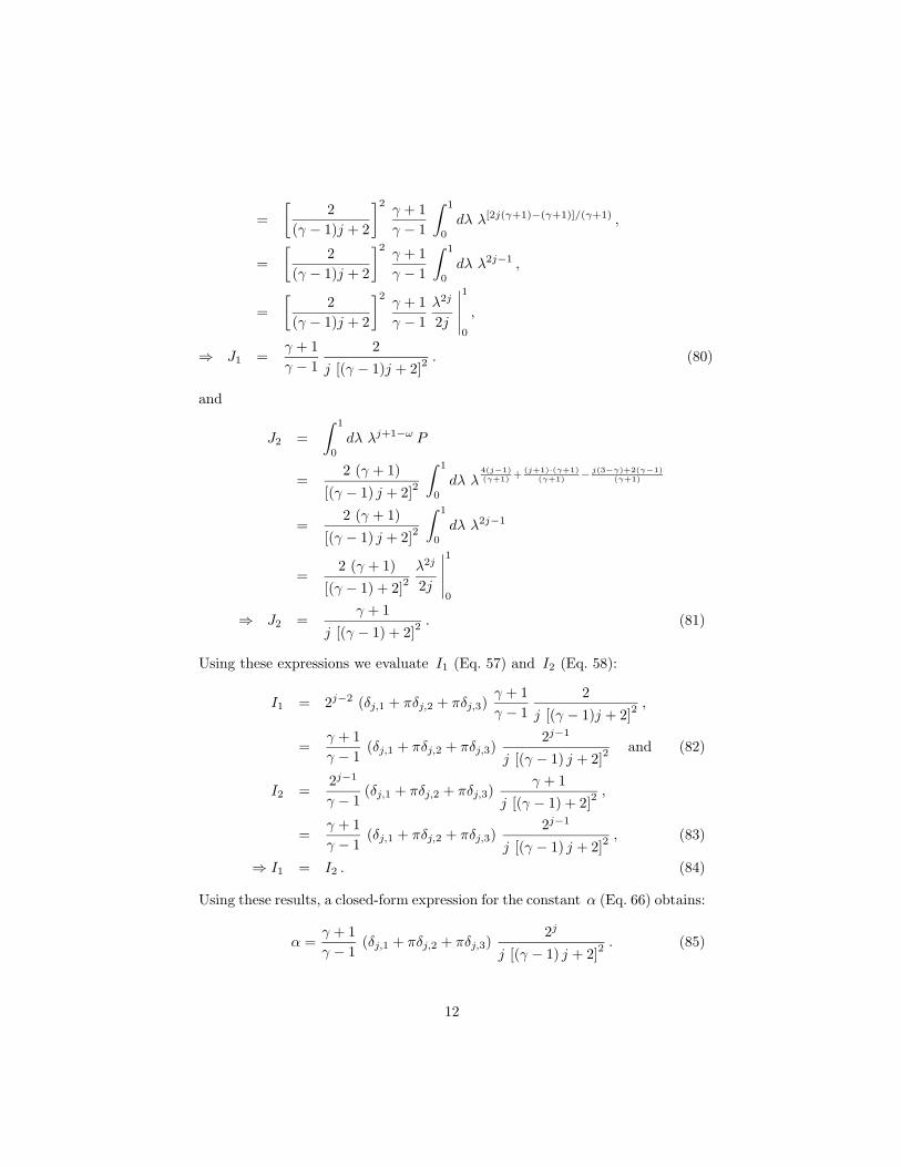
2(γ − 1)j + 2

]2γ + 1γ − 1

∫ 1

0

dλ λ[2j(γ+1)−(γ+1)]/(γ+1) ,

=[

2(γ − 1)j + 2

]2γ + 1γ − 1

∫ 1

0

dλ λ2j−1 ,

=[

2(γ − 1)j + 2

]2γ + 1γ − 1

λ2j

2j

∣∣∣∣∣1

0

,

⇒ J1 =γ + 1γ − 1

2j [(γ − 1)j + 2]2

. (80)

and

J2 =∫ 1

0

dλ λj+1−ω P

=2 (γ + 1)

[(γ − 1) j + 2]2

∫ 1

0

dλ λ4(j−1)(γ+1) +

(j+1)·(γ+1)(γ+1) − j(3−γ)+2(γ−1)

(γ+1)

=2 (γ + 1)

[(γ − 1) j + 2]2

∫ 1

0

dλ λ2j−1

=2 (γ + 1)

[(γ − 1) + 2]2λ2j

2j

∣∣∣∣∣1

0

⇒ J2 =γ + 1

j [(γ − 1) + 2]2. (81)

Using these expressions we evaluate I1 (Eq. 57) and I2 (Eq. 58):

I1 = 2j−2 (δj,1 + πδj,2 + πδj,3)γ + 1γ − 1

2j [(γ − 1)j + 2]2

,

=γ + 1γ − 1

(δj,1 + πδj,2 + πδj,3)2j−1

j [(γ − 1) j + 2]2and (82)

I2 =2j−1

γ − 1(δj,1 + πδj,2 + πδj,3)

γ + 1j [(γ − 1) + 2]2

,

=γ + 1γ − 1

(δj,1 + πδj,2 + πδj,3)2j−1

j [(γ − 1) j + 2]2, (83)

⇒ I1 = I2 . (84)

Using these results, a closed-form expression for the constant α (Eq. 66) obtains:

α =γ + 1γ − 1

(δj,1 + πδj,2 + πδj,3)2j

j [(γ − 1) j + 2]2. (85)

12

Further simplifications obtain in the singular case. Since V is constant(Eq. 19) and the closed-form expressions for both R and P are known (Eqs. 78and 79), the expressions given in Eq. 7 for the physical variables can be written

v =r

tV ∗, ρ =

A

rω

γ + 1γ − 1

λ4(j−1)/(γ+1), p =A

rω−2 t22 (γ + 1)

[(γ − 1) j + 2]2λ4(j−1)/(γ+1).

(86)We evaluate each of these expressions at the immediate post-shock state, anduse those results to obtain simplified expressions for these quantities.

For the velocity,

v2 =r2

tV ∗ ⇒ V ∗ =

tv2

r2. (87)

Substituting this result into the expression for v in Eq. 86 and using the ex-pression for λ in Eq. 8, we find that

v

v2=

r

tV ∗ × t

r2

1V ∗ =

r

r2

⇒ v

v2= λ . (88)

For the density, the post-shock state is

ρ2 =A

rω2

γ + 1γ − 1

(89)

so thatρ

ρ2=

A

rω

γ + 1γ − 1

λ4(j−1)/(γ+1) × rω2

A

γ − 1γ + 1

,

=(

r

r2

)−ω

λ4(j−1)/(γ+1) = λ4(j−1)

γ+1 −ω ,

= λ4j−4−3j+jγ−2γ+2

γ+1 = λj+jγ−2γ−2

γ+1 = λj(γ+1)−2(γ+1)

γ+1 ,

⇒ ρ

ρ2= λj−2 , (90)

where we have used Eq. 24 for ω.For the pressure, the post-shock state is

p2 =A

rω2

(r2

t

)2 2 (γ + 1)[(γ − 1) j + 2]2

. (91)

This result implies that

p

p2=

A

rω

(r

t

)2 2 (γ + 1)[(γ − 1) j + 2]2

λ4(j−1)/(γ+1) × rω2

A

(t

r2

)2 [(γ − 1) j + 2]2

2 (γ + 1)

=(

r

r2

)2−ω

λ4(j−1)/(γ+1) = λ4(j−1)

γ+1 −ω+2 ,

⇒ p

p2= λj . (92)

13

Using Eqs. 4, 90, and 92, it is a straightforward exercise to show that the SIEin the singular case varies quadratically with λ as

e

e2= λ2 . (93)

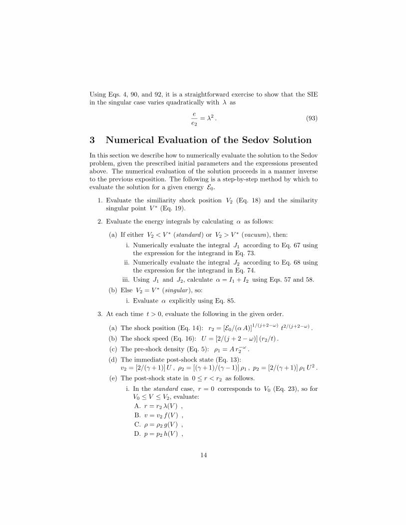
3 Numerical Evaluation of the Sedov Solution

In this section we describe how to numerically evaluate the solution to the Sedovproblem, given the prescribed initial parameters and the expressions presentedabove. The numerical evaluation of the solution proceeds in a manner inverseto the previous exposition. The following is a step-by-step method by which toevaluate the solution for a given energy E0.

1. Evaluate the similiarity shock position V2 (Eq. 18) and the similaritysingular point V ∗ (Eq. 19).

2. Evaluate the energy integrals by calculating α as follows:

(a) If either V2 < V ∗ (standard) or V2 > V ∗ (vacuum), then:

i. Numerically evaluate the integral J1 according to Eq. 67 usingthe expression for the integrand in Eq. 73.

ii. Numerically evaluate the integral J2 according to Eq. 68 usingthe expression for the integrand in Eq. 74.

iii. Using J1 and J2, calculate α = I1 + I2 using Eqs. 57 and 58.

(b) Else V2 = V ∗ (singular), so:

i. Evaluate α explicitly using Eq. 85.

3. At each time t > 0, evaluate the following in the given order.

(a) The shock position (Eq. 14): r2 = [E0/(α A)]1/(j+2−ω)t2/(j+2−ω) .

(b) The shock speed (Eq. 16): U = [2/(j + 2 − ω)] (r2/t) .

(c) The pre-shock density (Eq. 5): ρ1 = A r−ω2 .

(d) The immediate post-shock state (Eq. 13):v2 = [2/(γ + 1)]U , ρ2 = [(γ + 1)/(γ − 1)] ρ1 , p2 = [2/(γ + 1)] ρ1 U2 .

(e) The post-shock state in 0 ≤ r < r2 as follows.

i. In the standard case, r = 0 corresponds to V0 (Eq. 23), so forV0 ≤ V ≤ V2, evaluate:A. r = r2 λ(V ) ,B. v = v2 f(V ) ,C. ρ = ρ2 g(V ) ,D. p = p2 h(V ) ,

14

where λ, . . . , h are given in Eqs. 38–41.ii. In the singular case, although V has the unique value V ∗ (Eq. 19),

r = 0 corresponds to λ = 0 and r = r2 corresponds to λ = 1,so for 0 ≤ λ ≤ 1, evaluate (from Eqs. 88–92):A. r = r2 λ ,B. v = v2 λ ,C. ρ = ρ2 λj−2 ,D. p = p2 λj .

iii. In the vacuum case, r = rv corresponds to Vv (Eq. 28), sofor 0 ≤ r ≤ rv all quantities are zero, and for V2 ≤ V ≤ Vv,evaluate:A. r = r2 λ(V ) ,B. v = v2 f(V ) ,C. ρ = ρ2 g(V ) ,D. p = p2 h(V ) ,where λ, . . . , h are given in Eqs. 38–41.

4. The solution at a specific location r = r can be obtained as follows:

(a) In the standard and vacuum cases, identify the values of r (calculatedin step 3(e)iA) that bracket r and apply a root-finding routine (e.g.,zeroin [25]) to obtain the corresponding value V , from which theentire state can be calculated according to steps B–D of 3(e)i or3(e)iii.

(b) In the singular case, solve for the value of λ at r = r from Eq. 8,and obtain the remaining solution values from the relations given insteps B–D of 3(e)ii.

There are two sensitive computational issue in this procedure, both related tonumerical quadrature of steps 2(a)i and ii in the standard and vacuum cases.First, since the lower limit of the integral is a singular limit of the integrands,it should be augmented by a small amount to evaluate the integral. Second,empirical evidence suggests that different adaptive quadrature routines pro-vide slightly different answers in some circumstances. Anyone attempting toimplement this procedure is advised to carefully evaluate the results of thosenumerical quadratures.

4 Results

In this section we present results for the constant initial density (ω = 0) in §4.1and for the power-law initial density (ω �= 0) in §4.2. Results of the closed-formsolution are compared with results from the RAGE hydrocode [1] in §4.3.

15

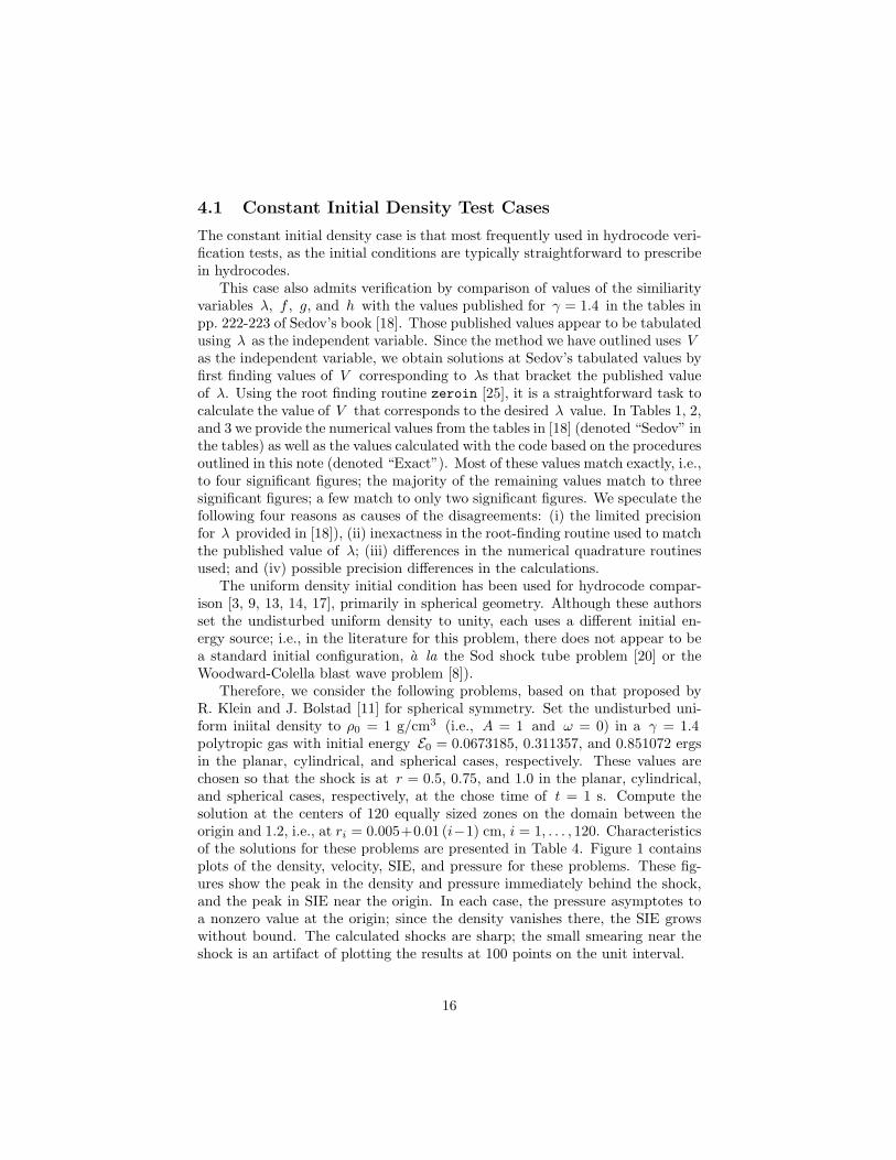
4.1 Constant Initial Density Test Cases

The constant initial density case is that most frequently used in hydrocode veri-fication tests, as the initial conditions are typically straightforward to prescribein hydrocodes.

This case also admits verification by comparison of values of the similiarityvariables λ, f , g, and h with the values published for γ = 1.4 in the tables inpp. 222-223 of Sedov’s book [18]. Those published values appear to be tabulatedusing λ as the independent variable. Since the method we have outlined uses Vas the independent variable, we obtain solutions at Sedov’s tabulated values byfirst finding values of V corresponding to λs that bracket the published valueof λ. Using the root finding routine zeroin [25], it is a straightforward task tocalculate the value of V that corresponds to the desired λ value. In Tables 1, 2,and 3 we provide the numerical values from the tables in [18] (denoted “Sedov” inthe tables) as well as the values calculated with the code based on the proceduresoutlined in this note (denoted “Exact”). Most of these values match exactly, i.e.,to four significant figures; the majority of the remaining values match to threesignificant figures; a few match to only two significant figures. We speculate thefollowing four reasons as causes of the disagreements: (i) the limited precisionfor λ provided in [18]), (ii) inexactness in the root-finding routine used to matchthe published value of λ; (iii) differences in the numerical quadrature routinesused; and (iv) possible precision differences in the calculations.

The uniform density initial condition has been used for hydrocode compar-ison [3, 9, 13, 14, 17], primarily in spherical geometry. Although these authorsset the undisturbed uniform density to unity, each uses a different initial en-ergy source; i.e., in the literature for this problem, there does not appear to bea standard initial configuration, a la the Sod shock tube problem [20] or theWoodward-Colella blast wave problem [8]).

Therefore, we consider the following problems, based on that proposed byR. Klein and J. Bolstad [11] for spherical symmetry. Set the undisturbed uni-form iniital density to ρ0 = 1 g/cm3 (i.e., A = 1 and ω = 0) in a γ = 1.4polytropic gas with initial energy E0 = 0.0673185, 0.311357, and 0.851072 ergsin the planar, cylindrical, and spherical cases, respectively. These values arechosen so that the shock is at r = 0.5, 0.75, and 1.0 in the planar, cylindrical,and spherical cases, respectively, at the chose time of t = 1 s. Compute thesolution at the centers of 120 equally sized zones on the domain between theorigin and 1.2, i.e., at ri = 0.005+0.01 (i−1) cm, i = 1, . . . , 120. Characteristicsof the solutions for these problems are presented in Table 4. Figure 1 containsplots of the density, velocity, SIE, and pressure for these problems. These fig-ures show the peak in the density and pressure immediately behind the shock,and the peak in SIE near the origin. In each case, the pressure asymptotes toa nonzero value at the origin; since the density vanishes there, the SIE growswithout bound. The calculated shocks are sharp; the small smearing near theshock is an artifact of plotting the results at 100 points on the unit interval.

16

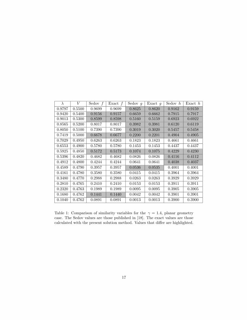
λ V Sedov f Exact f Sedov g Exact g Sedov h Exact h

0.9797 0.5500 0.9699 0.9699 0.8625 0.8620 0.9162 0.91590.9420 0.5400 0.9156 0.9157 0.6659 0.6662 0.7915 0.79170.9013 0.5300 0.8599 0.8598 0.5160 0.5159 0.6923 0.69220.8565 0.5200 0.8017 0.8017 0.3982 0.3981 0.6120 0.61190.8050 0.5100 0.7390 0.7390 0.3019 0.3020 0.5457 0.54580.7419 0.5000 0.6678 0.6677 0.2200 0.2201 0.4904 0.49050.7029 0.4950 0.6263 0.6263 0.1823 0.1823 0.4661 0.46610.6553 0.4900 0.5780 0.5780 0.1453 0.1453 0.4437 0.44370.5925 0.4850 0.5172 0.5173 0.1074 0.1075 0.4229 0.42300.5396 0.4820 0.4682 0.4682 0.0826 0.0826 0.4116 0.41120.4912 0.4800 0.4244 0.4244 0.0641 0.0641 0.4038 0.40370.4589 0.4790 0.3957 0.3957 0.0536 0.0535 0.4001 0.40010.4161 0.4780 0.3580 0.3580 0.0415 0.0415 0.3964 0.39640.3480 0.4770 0.2988 0.2988 0.0263 0.0263 0.3929 0.39290.2810 0.4765 0.2410 0.2410 0.0153 0.0153 0.3911 0.39110.2320 0.4763 0.1989 0.1989 0.0095 0.0095 0.3905 0.39050.1680 0.4762 0.1441 0.1440 0.0042 0.0042 0.3901 0.39010.1040 0.4762 0.0891 0.0891 0.0013 0.0013 0.3900 0.3900

Table 1: Comparison of similarity variables for the γ = 1.4, planar geometrycase. The Sedov values are those published in [18]. The exact values are thosecalculated with the present solution method. Values that differ are highlighted.

17


0.9998 0.4166 0.9996 0.9996 0.9973 0.9972 0.9985 0.99840.9802 0.4100 0.9645 0.9645 0.7653 0.7651 0.8659 0.86580.9644 0.4050 0.9374 0.9374 0.6285 0.6281 0.7832 0.78290.9476 0.4000 0.9097 0.9097 0.5164 0.5161 0.7124 0.71220.9295 0.3950 0.8812 0.8812 0.4234 0.4233 0.6514 0.65130.9096 0.3900 0.8514 0.8514 0.3451 0.3450 0.5983 0.59820.8725 0.3820 0.7998 0.7999 0.2427 0.2427 0.5266 0.52660.8442 0.3770 0.7638 0.7638 0.1892 0.1892 0.4884 0.48840.8094 0.3720 0.7226 0.7226 0.1414 0.1415 0.4545 0.45450.7629 0.3670 0.6720 0.6720 0.0975 0.0974 0.4242 0.42410.7242 0.3640 0.6327 0.6327 0.0718 0.0718 0.4074 0.40740.6894 0.3620 0.5989 0.5990 0.0545 0.0545 0.3969 0.39690.6390 0.3600 0.5521 0.5521 0.0362 0.0362 0.3867 0.38670.5745 0.3585 0.4943 0.4943 0.0208 0.0208 0.3794 0.37940.5180 0.3578 0.4448 0.4448 0.0123 0.0123 0.3760 0.37600.4748 0.3575 0.4073 0.4074 0.0079 0.0079 0.3746 0.37460.4222 0.3573 0.3621 0.3620 0.0044 0.0044 0.3737 0.37370.3654 0.3572 0.3133 0.3133 0.0021 0.0021 0.3733 0.37320.3000 0.3572 0.2571 0.2572 0.0008 0.0008 0.3730 0.37300.2500 0.3571 0.2143 0.2143 0.0003 0.0003 0.3729 0.37290.2000 0.3571 0.1714 0.1714 0.0001 0.0001 0.3729 0.37290.1500 0.3571 0.1286 0.1286 0.0000 0.0000 0.3729 0.37290.1000 0.3571 0.0857 0.0857 0.0000 0.0000 0.3729 0.3729

Table 2: Comparison of similarity variables for the γ = 1.4, cylindrical geometrycase. The Sedov values are those published in [18]. The exact values are thosecalculated with the present solution method. Values that differ are highlighted.

18


0.9913 0.3300 0.9814 0.9814 0.8379 0.8388 0.9109 0.91160.9773 0.3250 0.9529 0.9529 0.6457 0.6454 0.7993 0.79920.9622 0.3200 0.9237 0.9238 0.4978 0.4984 0.7078 0.70820.9342 0.3120 0.8744 0.8745 0.3241 0.3248 0.5923 0.59290.9080 0.3060 0.8335 0.8335 0.2279 0.2275 0.5241 0.52380.8747 0.3000 0.7872 0.7872 0.1509 0.1508 0.4674 0.46740.8359 0.2950 0.7397 0.7398 0.0967 0.0968 0.4272 0.42730.7950 0.2915 0.6952 0.6952 0.0621 0.0620 0.4021 0.40210.7493 0.2890 0.6496 0.6497 0.0379 0.0379 0.3856 0.38570.6788 0.2870 0.5844 0.5844 0.0174 0.0174 0.3732 0.37320.5794 0.2860 0.4971 0.4971 0.0052 0.0052 0.3672 0.36720.4560 0.2857 0.3909 0.3909 0.0009 0.0009 0.3656 0.36560.3600 0.2857 0.3086 0.3086 0.0002 0.0001 0.3655 0.36550.2960 0.2857 0.2538 0.2537 0.0000 0.0000 0.3655 0.36550.2000 0.2857 0.1714 0.1714 0.0000 0.0000 0.3655 0.36550.1040 0.2857 0.0892 0.0891 0.0000 0.0000 0.3655 0.3655

Table 3: Comparison of similarity variables for the γ = 1.4, spherical geometrycase. The Sedov values are those published in [18]. The exact values are thosecalculated with the present solution method. Values that differ are highlighted.

19

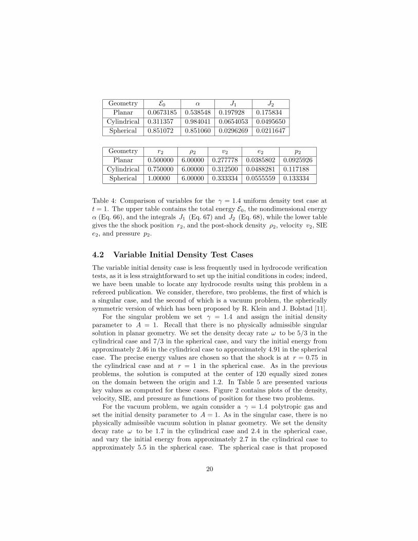
Geometry E0 α J1 J2

Planar 0.0673185 0.538548 0.197928 0.175834Cylindrical 0.311357 0.984041 0.0654053 0.0495650Spherical 0.851072 0.851060 0.0296269 0.0211647

Geometry r2 ρ2 v2 e2 p2

Planar 0.500000 6.00000 0.277778 0.0385802 0.0925926Cylindrical 0.750000 6.00000 0.312500 0.0488281 0.117188Spherical 1.00000 6.00000 0.333334 0.0555559 0.133334

Table 4: Comparison of variables for the γ = 1.4 uniform density test case att = 1. The upper table contains the total energy E0, the nondimensional energyα (Eq. 66), and the integrals J1 (Eq. 67) and J2 (Eq. 68), while the lower tablegives the the shock position r2, and the post-shock density ρ2, velocity v2, SIEe2, and pressure p2.

4.2 Variable Initial Density Test Cases

The variable initial density case is less frequently used in hydrocode verificationtests, as it is less straightforward to set up the initial conditions in codes; indeed,we have been unable to locate any hydrocode results using this problem in arefereed publication. We consider, therefore, two problems, the first of which isa singular case, and the second of which is a vacuum problem, the sphericallysymmetric version of which has been proposed by R. Klein and J. Bolstad [11].

For the singular problem we set γ = 1.4 and assign the initial densityparameter to A = 1. Recall that there is no physically admissible singularsolution in planar geometry. We set the density decay rate ω to be 5/3 in thecylindrical case and 7/3 in the spherical case, and vary the initial energy fromapproximately 2.46 in the cylindrical case to approximately 4.91 in the sphericalcase. The precise energy values are chosen so that the shock is at r = 0.75 inthe cylindrical case and at r = 1 in the spherical case. As in the previousproblems, the solution is computed at the center of 120 equally sized zoneson the domain between the origin and 1.2. In Table 5 are presented variouskey values as computed for these cases. Figure 2 contains plots of the density,velocity, SIE, and pressure as functions of position for these two problems.

For the vacuum problem, we again consider a γ = 1.4 polytropic gas andset the initial density parameter to A = 1. As in the singular case, there is nophysically admissible vacuum solution in planar geometry. We set the densitydecay rate ω to be 1.7 in the cylindrical case and 2.4 in the spherical case,and vary the initial energy from approximately 2.7 in the cylindrical case toapproximately 5.5 in the spherical case. The spherical case is that proposed

20

0

1

2

3

4

5

6

0 0.2 0.4 0.6 0.8 1 1.2

Den

sity

Position(a) Density.

0

0.1

0.2

0.3

0.4

0 0.2 0.4 0.6 0.8 1 1.2

Vel

ocity

Position(b) Velocity.

1E-21E-11E+01E+11E+21E+31E+41E+51E+61E+71E+81E+9

1E+10

0 0.2 0.4 0.6 0.8 1 1.2

Spec

ific

Int

erna

l Ene

rgy

Position(c) Specific Internal Energy.

0

0.05

0.1

0.15

0 0.2 0.4 0.6 0.8 1 1.2

Pres

sure

Position(d) Pressure.

Figure 1: Results of the γ = 1.4, uniform density test cases, corresponding toTable 4. Clockwise from the upper left are the density, velocity, pressure, andSIE for the planar (dotted), cylindrical (dashed), and spherical (solid) geome-tries, computed at 120 zones equally spaced on the domain [0,1.2].

21

0

2

4

6

8

10

0 0.2 0.4 0.6 0.8 1 1.2

Den

sity


0

0.2

0.4

0.6

0.8

0 0.2 0.4 0.6 0.8 1 1.2

Vel

ocity


1E-5

1E-4

1E-3

1E-2

1E-1

1E+0

0 0.2 0.4 0.6 0.8 1 1.2

Spec

ific

Int

erna

l Ene

rgy


0

0.1

0.2

0.3

0.4

0.5

0.6

0 0.2 0.4 0.6 0.8 1 1.2

Pres

sure


Figure 2: Results of the γ = 1.4, singular test cases at t = 1, corresponding toTable 5. Clockwise from the upper left are the density, velocity, pressure, andSIE for the cylindrical (dashed) and spherical (solid) geometries, computed at120 zones equally spaced on the domain [0,1.2].

22

Geometry E0 ω α

Cylindrical 2.45749 1.66667 4.80856Spherical 4.90875 2.33333 4.90875

Geometry r2 ρ2 v2 e2 p2

Cylindrical 0.75 9.69131 0.535714 0.143495 0.556261Spherical 1.00 6.00000 0.625000 0.195313 0.468750

Table 5: Comparison of variables for the γ = 1.4 singular test cases at t = 1.The upper table contains the total energy E0, the intial density exponent ω, andthe nondimensional energy α (Eq. 66), while the lower table gives the the shockposition r2, and the post-shock density ρ2, velocity v2, SIE e2, and pressurep2.

by R. Klein and J. Bolstad [11] as a hydrocode verification problem. As in theprevious problems, the solution is computed at the center of 120 equally sizedzones on the domain between the origin and 1.2. In Table 6 are presented variouskey values as computed for these cases. Figure 3 contains plots of the density,velocity, SIE, and pressure as functions of position for these two problems.

4.3 Hydrocode Comparisons

In this section we compare the some of the test cases described above withresults of the RAGE hydrocode [1]. In all cases, code results are for the 1Dspherical symmetry only. We first examine the uniform initial density case ofthe previous section. We then consider two cases with radially varying initialdensity: one being the singular case of the previous section, and the other beingthe vacuum case of the previous section.

4.3.1 Uniform Density Problem Comparison

We calculated the 1D spherical test problem given in Table 4 with RAGE. Theproblem was on the domain [0, 1.2], and run to a final time of t = 1. Graphicalresults of this case are given in Fig. 4 for 120 zones on [0, 1.2] and Fig. 5 for960 zones on [0, 1.2]. These figures show the density, velocity, SIE, and pressurefrom RAGE (dashed line) as well as the “exact” solution (solid line), plottedagainst the left axis, in addition to the absolute difference between these values(dotted line), plotted against the right axis.

The disagreement between the exact and hydrocode solutions is notable,particularly in the vicinity of the shock. We speculate that this error is largelydue to the fact that in the hydrocode calculation, the initial energy is deposited

23

0

2

4

6

8

10

12

14

16

0 0.2 0.4 0.6 0.8 1 1.2

Den

sity


0

0.1

0.2

0.3

0.4

0.5

0.6

0.7

0 0.2 0.4 0.6 0.8 1 1.2

Vel

ocity


1E-4

1E-3

1E-2

1E-1

1E+0

0 0.2 0.4 0.6 0.8 1 1.2

Spec

ific

Int

erna

l Ene

rgy


0

0.1

0.2

0.3

0.4

0.5

0.6

0 0.2 0.4 0.6 0.8 1 1.2

Pres

sure


Figure 3: Results of the γ = 1.4, vacuum test cases at t = 1, corresponding toTable 6. Clockwise from the upper left are the density, velocity, pressure, andSIE for the cylindrical (dashed) and spherical (solid) geometries, computed at120 zones equally spaced on the domain [0,1.2].

24

Geometry E0 ω α J1 J2

Cylindrical 2.67315 1.70 5.18062 0.856238 0.158561Spherical 5.45670 2.40 5.45670 0.454265 0.0828391

Geometry rv r2 ρ2 v2 e2 p2

Cylindrical 0.154090 0.750000 9.78469 0.543478 0.147684 0.578018Spherical 0.272644 1.00000 6.00000 0.641026 0.205457 0.493097

Table 6: Comparison of variables for the γ = 1.4 vacuum test cases at t = 1.The upper table contains the total energy E0, the intial density exponent ω,the nondimensional energy α (Eq. 66), and the integrals J1 (Eq. 67) and J2

(Eq. 68), while the lower table gives the vacuum boundary position rv, shockposition r2, and the post-shock density ρ2, velocity v2, SIE e2, and pressurep2.

in the zone nearest the origin; that is, it is not a true delta-function initialcondition. We surmise that the finite nature of the hydrocode initial conditionimprints on the subsequent dynamics, leading to values that differ somewhatfrom those of the exact solution.

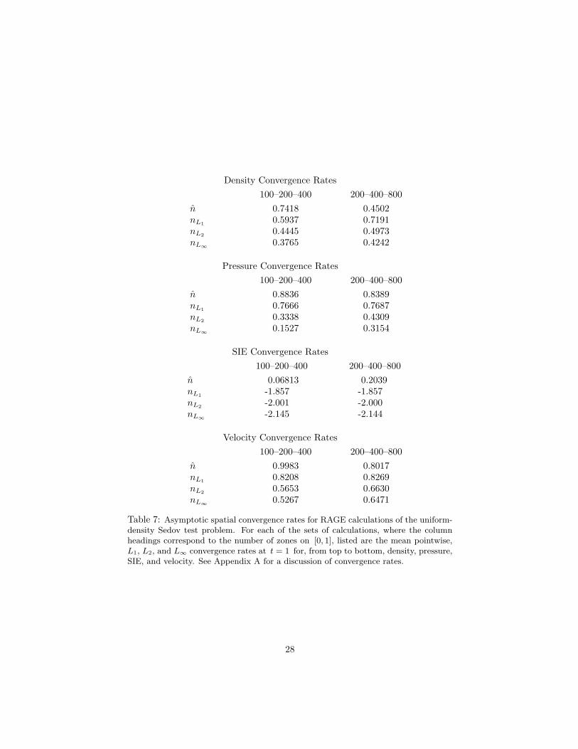
Comparison of these two figures gives some notion of the convergence ofthe calculation under grid refinement. This concept is rigorously quantified inTable 7, which gives asymptotic spatial convergence rates1 for RAGE calcula-tions with 120-240-480 zones and 240-480-960 zones. We include four conver-gence rates: mean, L1, L2, L∞; typically, the L1 convergence rate is used forproblems with shocks. For these variables, all convergence rates are sublinear;indeed, the SIE convergence rates appear anomalous. From these results, it isclear that the calculation is converging.

1See Appendix A for a discussion of convergence rates and how they are calculated.

25

0

1

2

3

4

5

6

7

8

1E-7

1E-6

1E-5

1E-4

1E-3

1E-2

1E-1

1E+0

1E+1

0 0.2 0.4 0.6 0.8 1 1.2

Den

sity

|Den

sity

Dif

fere

nce|


0

0.05

0.1

0.15

0.2

0.25

0.3

0.35

1E-7

1E-6

1E-5

1E-4

1E-3

1E-2

1E-1

1E+0

0 0.2 0.4 0.6 0.8 1 1.2

Vel

ocity

|Vel

ocity

Dif

fere

nce|


1E-41E-31E-21E-11E+01E+11E+21E+31E+41E+51E+61E+71E+81E+9

1E+10

1E-41E-31E-21E-11E+01E+11E+21E+31E+41E+51E+61E+71E+81E+91E+10

0 0.2 0.4 0.6 0.8 1 1.2

Spec

ific

Int

erna

l Ene

rgy

|SIE

Dif

fere

nce|


0

0.03

0.06

0.09

0.12

0.15

1E-5

1E-4

1E-3

1E-2

1E-1

1E+0

0 0.2 0.4 0.6 0.8 1 1.2

Pres

sure

|Pre

ssur

e D

iffe

renc

e|


Figure 4: Results of RAGE on the 1D, spherical, γ = 1.4, uniform density testcase with total energy E0 = 0.851072, corresponding to Table 4. Clockwise fromthe upper left are the density, velocity, pressure, and SIE for RAGE (dashed)and the exact (solid) solutions, both plotted against the left axis, as well as theabsolute difference (dotted), plotted against the right axis. Both solutions werecalculated at the centers of 120 zones equally spaced on the domain [0, 1.2].

26

0

1

2

3

4

5

6

7

8

1E-7

1E-6

1E-5

1E-4

1E-3

1E-2

1E-1

1E+0

1E+1

0 0.2 0.4 0.6 0.8 1 1.2

Den

sity

|Den

sity

Dif

fere

nce|


0

0.05

0.1

0.15

0.2

0.25

0.3

0.35

1E-7

1E-6

1E-5

1E-4

1E-3

1E-2

1E-1

1E+0

0 0.2 0.4 0.6 0.8 1 1.2

Vel

ocity

|Vel

ocity

Dif

fere

nce|


1E-41E-31E-21E-11E+01E+11E+21E+31E+41E+51E+61E+71E+81E+9

1E+10

1E-41E-31E-21E-11E+01E+11E+21E+31E+41E+51E+61E+71E+81E+91E+10

0 0.2 0.4 0.6 0.8 1 1.2

0 0.2 0.4 0.6 0.8 1 1.2

Spec

ific

Int

erna

l Ene

rgy

|SIE

Dif

fere

nce|


0

0.03

0.06

0.09

0.12

0.15

1E-5

1E-4

1E-3

1E-2

1E-1

1E+0

0 0.2 0.4 0.6 0.8 1 1.2

Pres

sure

|Pre

ssur

e D

iffe

renc

e|


Figure 5: Results of RAGE on the 1D, spherical, γ = 1.4, uniform density testcase with total energy E0 = 0.851072, corresponding to Table 4. Clockwise fromthe upper left are the density, velocity, pressure, and SIE for RAGE (dashed)and the exact (solid) solutions, both plotted against the left axis, as well as theabsolute difference (dotted), plotted against the right axis. Both solutions werecalculated at the centers of 960 zones equally spaced on the domain [0, 1.2].

27

Density Convergence Rates100–200–400 200–400–800

n 0.7418 0.4502nL1 0.5937 0.7191nL2 0.4445 0.4973nL∞ 0.3765 0.4242

Pressure Convergence Rates100–200–400 200–400–800

n 0.8836 0.8389nL1 0.7666 0.7687nL2 0.3338 0.4309nL∞ 0.1527 0.3154

SIE Convergence Rates100–200–400 200–400–800

n 0.06813 0.2039nL1 -1.857 -1.857nL2 -2.001 -2.000nL∞ -2.145 -2.144

Velocity Convergence Rates100–200–400 200–400–800

n 0.9983 0.8017nL1 0.8208 0.8269nL2 0.5653 0.6630nL∞ 0.5267 0.6471

Table 7: Asymptotic spatial convergence rates for RAGE calculations of the uniform-density Sedov test problem. For each of the sets of calculations, where the columnheadings correspond to the number of zones on [0, 1], listed are the mean pointwise,L1, L2, and L∞ convergence rates at t = 1 for, from top to bottom, density, pressure,SIE, and velocity. See Appendix A for a discussion of convergence rates.

28

4.3.2 Singular Problem Comparison

We next consider the 1D spherical singular test problem described in Table 5,with results previously shown in Fig. 2. The problem is on the domain [0, 1.2],and run to a final time of t = 1. Graphical results of this case are given inFig. 6 for 120 zones on [0, 1.2] and Fig. 7 for 960 zones on [0, 1.2]. These figuresshow the density, velocity, SIE, and pressure from RAGE (dashed line) as wellas the “exact” solution (solid line), plotted against the left axis, in addition tothe absolute difference between these values (dotted line), plotted against theright axis.

The code results exhibit singificant errors in the region near the origin, which,in this case, should have linearly vanishing density and velocity as the originis approached. Examination of results at earlier times suggest an inability ofthe hydrodynamics algorithm to move the initial high density, high energy ma-terial out of the near-origin zone; this incorrect mass distribution leading to aseries of reflected and converging waves that pollute the solution at later time.Comparison of Figs. 6 and 7, however, suggests improvement, albeit slow, undermesh refinement, particularly adjacent to the shock. Additionally, all quantitiesdecrease by approximately a factor of two with the eightfold increase in zoningin the vicinity of the origin. Less extensive testing of other hydrocodes [12, 15],both Eulerian and Lagrangian, on this problem revealed similar difficulties.

Calculated asymptotic convergence rates for this problem are provided inTable 8. RAGE calculations with 120-240-480 zones and 240-480-960 zones on[0, 1.2] were used in those calculations. Those results suggest that the 120-240-480 zone calculations are not within the domain of asymptotic convergence,while the 240-480-960 zone set may be. It is unclear from those convergencerate values if the code results are approaching the exact solution.

29

0

2

4

6

8

1E-3

1E-2

1E-1

1E+0

1E+1

0 0.2 0.4 0.6 0.8 1 1.2

Den

sity

|Den

sity

Dif

fere

nce|


0

0.2

0.4

0.6

0.8

1

1E-5

1E-4

1E-3

1E-2

1E-1

1E+0

0 0.2 0.4 0.6 0.8 1 1.2

Vel

ocity

|Vel

ocity

Dif

fere

nce|


1E-5

1E-4

1E-3

1E-2

1E-1

1E+0

1E-5

1E-4

1E-3

1E-2

1E-1

1E+0

0 0.2 0.4 0.6 0.8 1 1.2

Spec

ific

Int

erna

l Ene

rgy

|SIE

Dif

fere

nce|


0

0.1

0.2

0.3

0.4

0.5

1E-5

1E-4

1E-3

1E-2

1E-1

1E+0

0 0.2 0.4 0.6 0.8 1 1.2

Pres

sure

|Pre

ssur

e D

iffe

renc

e|


Figure 6: Results of RAGE on the 1D, spherical, γ = 1.4, singular test casewith total energy E0 = 5.45670 and initial density ρ0(r) = r−2.4, correspondingto Table 6. Clockwise from the upper left are the density, velocity, pressure, andSIE for RAGE (dashed) and the exact (solid) solutions, both plotted againstthe left axis, as well as the absolute difference (dotted), plotted against the rightaxis. Both solutions were calculated at the centers of 120 zones equally spacedon the domain [0, 1.2].

30

0

2

4

6

8

1E-3

1E-2

1E-1

1E+0

1E+1

0 0.2 0.4 0.6 0.8 1 1.2

Den

sity

|Den

sity

Dif

fere

nce|


0

0.2

0.4

0.6

0.8

1

1E-5

1E-4

1E-3

1E-2

1E-1

1E+0

0 0.2 0.4 0.6 0.8 1 1.2

Vel

ocity

|Vel

ocity

Dif

fere

nce|


1E-5

1E-4

1E-3

1E-2

1E-1

1E+0

1E-5

1E-4

1E-3

1E-2

1E-1

1E+0

0 0.2 0.4 0.6 0.8 1 1.2

Spec

ific

Int

erna

l Ene

rgy

|SIE

Dif

fere

nce|


0

0.1

0.2

0.3

0.4

0.5

1E-5

1E-4

1E-3

1E-2

1E-1

1E+0

0 0.2 0.4 0.6 0.8 1 1.2

Pres

sure

|Pre

ssur

e D

iffe

renc

e|


Figure 7: Results of RAGE on the 1D, spherical, γ = 1.4, singular test casewith total energy E0 = 5.45670 and initial density ρ0(r) = r−2.4, correspondingto Table 6. Clockwise from the upper left are the density, velocity, pressure, andSIE for RAGE (dashed) and the exact (solid) solutions, both plotted againstthe left axis, as well as the absolute difference (dotted), plotted against the rightaxis. Both solutions were calculated at the centers of 960 zones equally spacedon the domain [0, 1.2].

31


n -0.07694 0.6900nL1 -0.06701 0.5189nL2 -0.01540 0.3732nL∞ 0.7123 0.2035


n 0.8416 1.052nL1 0.4893 1.018nL2 0.4713 0.7224nL∞ 0.8318 0.4668


n 0.3060 0.3862nL1 0.3483 0.6141nL2 0.2216 0.5260nL∞ -0.03705 0.3919


n 2.278 0.9676nL1 1.999 -0.5057nL2 0.6335 0.2806nL∞ -0.3283 0.4418

Table 8: Asymptotic spatial convergence rates for RAGE calculations of the Sedovsingular problem. For each of the sets of calculations, where the column headingscorrespond to the number of zones on [0, 1], listed are the mean pointwise, L1, L2,and L∞ convergence rates at t = 1 for, from top to bottom, density, pressure, SIE,and velocity. See Appendix A for a discussion of convergence rates.

32

4.3.3 Vacuum Problem Comparison

Lastly, we consider the 1D spherical vacuum problem given in Table 6 and shownin Fig. 3. The problem was on the domain [0, 1.2], and run to a final time oft = 1. Graphical results of this case are given in Fig. 8 for 120 zones on [0, 1.2]and Fig. 9 for 960 zones on [0, 1.2]. These figures show the density, velocity, SIE,and pressure from RAGE (dashed line) as well as the “exact” solution (solidline), plotted against the left axis, in addition to the absolute difference betweenthese values (dotted line), plotted against the right axis.

These results exhibit behavior similar to that of the singular case, namely,the inability to resolve the region near the origin, which, in this case should havevanishingly small density. Indeed, the entire vacuum region is poorly resolvedin all of these calculations. As in the previous case, comparison of Figs. 8 and9, however, shows improvement under mesh refinement, particularly near theshock. Improvement is also seen in the vacuum region, where, e.g., the error inboth the density and pressure decreases by ∼50% with the eightfold increase inzones. Closer analysis of these calculations shows the same phenomenon as inthe singular case, viz., the inability of the hydrodynamics algorithms to movethe initial high density, high energy material out of the near-origin zone earlyin the calculation. This is the same pathological initial-condition imprinting asin the singular case. Less extensive testing of other hydrocodes [4, 12, 15], bothEulerian and Lagrangian, on this problem revealed similar difficulties.

Calculated asymptotic convergence rates for this problem are provided inTable 9. As in the singular case, these results suggest that the 120-240-480zone calculations are not within the domain of asymptotic convergence, whilethe 240-480-960 zone set may be; the low convergence rates for density in thatcase suggest that it is not the case for that variable. It is unclear from thoseconvergence rate values if the code results are approaching the exact solution inthe vicinity of the vacuum region (in general) and the origin (in particular).

33

0

1

2

3

4

5

6

7

0

0.5

1

1.5

2

2.5

3

3.5

0 0.2 0.4 0.6 0.8 1 1.2

Den

sity

|Den

sity

Dif

fere

nce|


0

0.2

0.4

0.6

0.8

1E-4

1E-3

1E-2

1E-1

1E+01E+0

0 0.2 0.4 0.6 0.8 1 1.2

Vel

ocity

|Vel

ocity

Dif

fere

nce|


0

0.05

0.1

0.15

0.2

0.25

1E-5

1E-4

1E-3

1E-2

1E-1

1E+0

0 0.2 0.4 0.6 0.8 1 1.2

Spec

ific

Int

erna

l Ene

rgy

|SIE

Dif

fere

nce|


0

0.1

0.2

0.3

0.4

0.5

1E-5

1E-4

1E-3

1E-2

1E-1

1E+0

0 0.2 0.4 0.6 0.8 1 1.2

Pres

sure

|Pre

ssur

e D

iffe

renc

e|


Figure 8: Results of RAGE on the 1D, spherical, γ = 1.4, vacuum test casewith total energy E0 = 5.45670 and initial density ρ0(r) = r−2.4, correspondingto Table 6. Clockwise from the upper left are the density, velocity, pressure, andSIE for RAGE (dashed) and the exact (solid) solutions, both plotted againstthe left axis, as well as the absolute difference (dotted), plotted against the rightaxis. Both solutions were calculated at the centers of 120 zones equally spacedon the domain [0, 1.2].

34

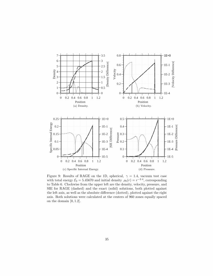
0

1

2

3

4

5

6

7

0

0.5

1

1.5

2

2.5

3

3.5

0 0.2 0.4 0.6 0.8 1 1.2

Den

sity

|Den

sity

Dif

fere

nce|


0

0.2

0.4

0.6

0.8

1E-4

1E-3

1E-2

1E-1

1E+01E+0

0 0.2 0.4 0.6 0.8 1 1.2

Vel

ocity

|Vel

ocity

Dif

fere

nce|


0

0.05

0.1

0.15

0.2

0.25

1E-5

1E-4

1E-3

1E-2

1E-1

1E+0

0 0.2 0.4 0.6 0.8 1 1.2

Spec

ific

Int

erna

l Ene

rgy

|SIE

Dif

fere

nce|


0

0.1

0.2

0.3

0.4

0.5

1E-5

1E-4

1E-3

1E-2

1E-1

1E+0

0 0.2 0.4 0.6 0.8 1 1.2

Pres

sure

|Pre

ssur

e D

iffe

renc

e|


Figure 9: Results of RAGE on the 1D, spherical, γ = 1.4, vacuum test casewith total energy E0 = 5.45670 and initial density ρ0(r) = r−2.4, correspondingto Table 6. Clockwise from the upper left are the density, velocity, pressure, andSIE for RAGE (dashed) and the exact (solid) solutions, both plotted againstthe left axis, as well as the absolute difference (dotted), plotted against the rightaxis. Both solutions were calculated at the centers of 960 zones equally spacedon the domain [0, 1.2].

35


n -0.08326 0.2131nL1 -0.03525 0.1283nL2 0.05707 0.08358nL∞ 0.6052 0.05947


n 0.3482 1.083nL1 0.5212 0.8079nL2 0.8615 0.6551nL∞ 0.9804 0.5647


n 0.4526 0.4567nL1 0.3373 0.5270nL2 0.2298 0.4519nL∞ -0.8449 0.5123


n 0.4771 1.546nL1 0.04443 1.416nL2 0.01945 0.8952nL∞ 0.4351 0.4692

Table 9: Asymptotic spatial convergence rates for RAGE calculations of the Sedovvacuum problem. For each of the sets of calculations, where the column headingscorrespond to the number of zones on [0, 1], listed are the mean pointwise, L1, L2,and L∞ convergence rates at t = 1 for, from top to bottom, density, pressure, SIE,and velocity. See Appendix A for a discussion of convergence rates.

36

5 Summary

We have reviewed Sedov’s solution, given in [18], for the problem of self-similar,one-dimensional, compressible hydrodynamics in which a finite amount of energyis released at the origin at the initial time. The main result of this report is givenin §3, where we outline an algorithmic procedure for evaluating this solution,in terms of quantities and equations found primarily in §2, which contains anelaboration of Sedov’s solution. In addition to the “standard Sedov problem,”we have included the solution to the singular and vacuum problems in bothcylindrical and spherical geometries.

In §4 we showed examples of these solutions. Such problems can be usedin the verification of hydrodynamics codes. Computed asymptotic convergencerates based on hydrocode calculations of these problems showed sublinear con-vergence at best; calculations of the singular and vacuum did not converge onthe coarsest grids (100-200-400 zones on the unit interval). We also comparedhydrocode calculations with the exact solutions. Those comparisons suggestthat the Godunov-type high-resolution method used in the RAGE hydrocodeperforms adequately on the standard Sedov problem, but may perform inade-quately on problems for which the pressure vanishes at the origin. Althoughwe have presented only RAGE results herein, less extensive testing of other hy-drocodes [4, 12, 15], both Eulerian and Lagrangian, revealed similar difficultiesfor problems in which the pressure vanishes at and near the origin. Althoughthe magnitude of the error in the vicinity of the origin diminishes under mesh re-finement, we make the heuristic albeit plausible speculation that the hydrocodesolution may not be not converging to the exact solution for these problems.We speculate that a possible fundamental shortcoming of present hydrodynamicintegration methods for these highly singular flows may be uncovered by a thor-ough investigation of the singular and vacuum Sedov problems.

37

Acknowledgments

The careful reviews by Rob Lowrie and Bill Rider are kindly acknowledged.This work was performed by Los Alamos National Laboratory, which is operatedby the University of California for the U.S. Department of Energy under contractW-7405-ENG-36.

38

References

[1] R. M. Baltrusaitis, M. L. Gittings, R. P. Weaver, R. P. Benjamin &J. M. Budzinski, Simulation of shock-generated instabilities, Phys. Flu-ids 8(9), pp. 2471–2483 (1996).

[2] J. Bolstad, LLNL, personal communication.

[3] J.R. Buchler, Z. Kollath & A. Marom, An Adaptive Code for Radial StellarModel Pulsations, Astrophys. Space Sci. 253, pp. 139–160 (1997).

[4] M. Clover, LANL, personal communication.

[5] S.V. Coggeshall, “Group-invariant Solutions of Hydrodynamics”, in Com-putational Fluid Dynamics: Selected Topics, K.G. Roesner, D. Leutloff &R.C. Srivastava, eds., Springer, New York pp. 71–101 (1995).

[6] S.V. Coggeshall & R.A. Axford, Lie group invariance properties of radiationhydrodynamics equations and their associated similarity solutions, Phys.Fluids 29(8), pp. 2398–2420 (1986).

[7] S.V. Coggeshall & J. Meyer-ter-Vehn, Group-invariant solutions of and op-timal systems for multidimensional hydrodynamics, J. Math. Phys. 31(10),pp. 3585–3601 (1992).

[8] P. Colella & P. R. Woodward, The Piecewise Parabolic Method (PPM) forGas-dynamical Simulations, J. Comp. Phys. 54, pp. 174–201 (1984).

[9] B. Fryxell, K. Olson, P. Ricker, R.X. Timmes, M. Zingale, D.Q. Lamb,P. MacNeice, R. Rosner, J.W. Truran & H. Tufo, FLASH: An Adap-tive Mesh Hydrodynamics Code for Modeling Astrophysical ThermonuclearFlashes, Astrophys. J. Suppl. Ser. 131, pp. 273–334 (2000).

[10] J. R. Kamm & W. J. Rider, 2-D Convergence Analysis of the RAGE Hy-drocode, Los Alamos National Laboratory Report LA-UR-98-3872 (1998).

[11] R. Klein & J. Bolstad, LLNL, personal communication.

[12] R. Lowrie, LANL, personal communication.

[13] J.M. Owen, J.V. Villumsen, P.R. Shapiro & H. Martel, Adaptive SmoothedParticle Hydrodynamics: Methodology. II., Astrophys. J. Supp. Ser. 116,pp. 155–209 (1998).

[14] C. Reile & T. Gehren, Numerical simulation of photospheric convectionin solar-type stars I. Hydrodynamical test calculations, Astron. Astro-phys. 242, pp. 142–174 (1991).

[15] W. Rider, LANL, personal communication.

39

[16] R. Reinicke & J. Meyer-ter-Vehn, The point explosion with heat conduc-tion, Phys. Fluids A 3(7), pp. 1807–1818 (1991).

[17] M. Shashkov & B. Wendroff, A Composite Scheme for Gas Dynamics inLagrangian Coordinates, J. Comp. Phys. 150, pp. 502–517 (1999).

[18] L.I. Sedov, Similarity and Dimensional Methods in Mechanics, AcademicPress, New York, NY, p. 147 ff. (1959).

[19] A.I. Shestakov, Time-dependent simulations of point explosions with heatconduction, Phys. Fluids 11(5), pp. 1091-1095 (1999).

[20] G. Sod, A survey of several finite difference methods for systems of nonlin-ear hyperbolic conservation laws, J. Comp. Phys. 27, pp. 1–31 (1978).

[21] G.I. Taylor, The formation of a blast wave by a very intense explosion,Proc. Roy. Soc. London A 201, pp. 159-174 (1950).

[22] H.A Bethe, K. Fuchs, J.O. Hirschfelder, J.L. Magee, R.E. Peierls, J. vonNeumann, Blast Wave, Los Alamos Scientific Laboratory Report LA-2000,August 1947.

[23] G.B. Whitham, Linear and Nonlinear Waves, John Wiley & Sons, NewYork, NY, p. 177 (1974).

[24] The quadrature routines in ACM agorithm 691 are available from Netlibat http://www.netlib.org/.

[25] The zeroin routine is availabe from Netlib at http://www.netlib.org/.

40

A Spatial Convergence Analysis

For any variable ξ computed at a given uniform grid spacing ∆x, the funda-mental Ansatz of convergence analysis is that the difference between the exactand computed solutions can be expanded as a polynomial function of the gridspacing:

ξ∗ − ξi = A (∆xi)τ + o

((∆xi)

n)

, (A1)

where ξ∗ is the exact value, ξi is the value computed on the grid of spacing∆xi, A is the convergence coefficient , and τ is the convergence rate. Using thesolution on three different grids, related by a uniform mesh ratios, one obtains

τ =log [(ξm − ξc) / (ξf − ξm)]

log ς,

A = − ξf − 2ξm + ξc

(∆x)τ (ς−τ − 1)2, (A2)

where the subscripts c, m, and f refer to the coarse-, medium-, and fine-gridsolutions, respectively, and ς is the uniform ratio of the medium-to-coarse gridsand fine-to-medium grids. To apply these results computationally, the data onthe medium and fine grids must be averaged onto the coarse grid. Typically,the ratio of grid sizes is taken to be two, and the following procedure is applied:the volume-weighted means of the two bracketing values of the medium solutionand the four bracketing values of the fine solution are calculated and used asthe cell-averaged values at the corresponding coarse gridpoint. For example,using density as the variable of interest and assuming the coarse grid has Npoints, values ρm

i′ from the i′th zone (which has volume V mi′ ) of the medium-

grid solution, i′ = 1, . . . , 2N , are interpolated to the value ρc←mi at locations

xi, i = 1, . . . , N , on the coarse grid as

ρc←mi =

(V m

2i−1ρm2i−1 + V m

2i ρm2i

)/

(V m

2i−1 + V m2i

). (A3)

Similarly, values from the fine solution, ρfı , ı = 1, . . . , 4N , are interpolated to

the locations ρc←fi at the corresponding position on the coarse grid as

ρc←fi =

V f4i−3ρ

f4i−3 + V f

4i−2ρf4i−2 + V f

4i−1ρf4i−1 + V f

4iρf4i

V f4i−3 + V f

4i−2 + V f4i−1 + V f

4i

. (A4)

These values are used in Eq. A2 to determine the pointwise convergence char-acteristics.

With the pointwise convergence rates, a mean convergence rate over theentire domain is constructed by taking the arithmetic average of the (local)convergence rate at each gridpoint, i.e.,

τ =1N

∑i

τi , (A5)

41

where τi is the asymptotic convergence rate computed at gridpoint xi, i =1, . . . , N . We indicate the total number of points in this average as N notas N , for the reason that all points on the computational grid might not beused in the evaluation of the mean pointwise convergence rate. For example, ifthe numerical values of the cell-averaged quantities from the fine and mediummeshes are identical, then the expression for τ in Eq. A2 either diverges (if thosevalues do not equal the value on the coarse mesh) or is undefined (if all valuesare identical). Similarly, the computed value of the argument of the logarithmin the numerator of Eq. A2 could be negative, leading to an imaginary value forτ . We include only well-defined pointwise convergence rates in Eq. A5 and findthat, in general, N �= N .

The asymptotic convergence rate can also be computed with a global quan-tity. For example, the convergence rate for the norm of a computed quantityover the entire grid is given as

τ.=

log [||ξm − ξc||/||ξf − ξm||]log ς

, (A6)

where || · || denotes any consistent norm. For the global rates, we compute theL1, L2, and L∞ norms in Eq. A6; using density as the variable of interest andthe difference between values on the medium and coarse grids, these norms aredefined as

||ρm − ρc||1 ≡ 1N

∑i

∣∣ρmi − ρc

i

∣∣ , (A7)

||ρm − ρc||2 ≡√

1N

∑i

∣∣ρmi − ρc

i

∣∣2 , (A8)

||ρm − ρc||∞ ≡ maxi

{∣∣ρmi − ρc

i

∣∣} , (A9)

where N is the number of gridpoints, and ρmi and ρc

i are the density at xi

computed on the medium grid (interpolated to the coarse grid) and coarse grids,respectively. For the global convergence rate based on norms, all of the pointsin the domain of interest are perforce included in the evaluation of the norms,and, therefore, in the evaluation of the convergence rate. It is possible (thoughunlikely) that one or both of the norms in the numerator of the RHS of Eq. A6could equal zero; in such a case, the convergence rate is undefined.

42

evaluation of the sedov-von neumann-taylor blast wave...

Documents