evaluation of the effects of ionizing radiation in iter’s · evaluation of the effects of...
TRANSCRIPT

Evaluation of the effects of ionizing radiation in ITER’s
Plasma Position Reflectometry System
Laura Estévez Núñez
Thesis for the degree of Master in
Mechanical Engineering
Supervisors: Dr. Raul Fernandes Luís
Dr. Hugo Filipe Diniz Policarpo
Examination Committee
Chairperson: Prof. Mário Manuel Gonçalves da Costa
Supervisor: Dr. Raul Fernandes Luís
Member of the Committee: Dr. Yuriy Romanets
October 2016

II
TO MY FAMILY

III
ACKNOWLEDGEMENTS
I would like to extremely thank to all the people whose names might not be enumerated and organisms
that have contributed and made possible for me to do this exciting undertaking.
First of all, I express my deeply gratitude to my supervisors. Without them I could have not achieved a
good level of motivation and learning on the topic. I could not be more satisfied with Hugo Policarpo and
Raul Luís for their guidance, patience, kindness, endless encouragement and attention.
I would also like to thank my colleagues in the Instituto de Plasmas e Fusão Nuclear (IPFN), who have
aided me in the understanding of the programs used, and the International Offices of the IST and ETSII
for giving me the chance to do this passionate master thesis abroad and be able to grow personally.
Moreover, I would like to specially thank to Professor Miguel Tavares da Silva for giving me the chance
of doing the master thesis in the area I was looking for. I appreciate he put me into contact with my
supervisors from the IST.
Finally, my family and friends have been decisive in the making of the project. They have given me all
kind of unconditional support for which I will be eternally grateful.

IV
RESUMO
No ITER (International Thermonuclear Experimental Reactor), o sistema de Reflectometria de Posição
de Plasma (PPR) estará exposto a elevados níveis de radiação ionizante: neutrões provenientes das
reações de fusão nuclear e fotões gerados nas interações nucleares com os materiais circundantes. O
principal objectivo desta Tese é contribuir para o estudo do efeito das cargas nucleares nos
componentes do sistema PPR através de cálculos de deposição de energia, complementando cálculos
de distribuição de temperaturas efectuados em trabalhos anteriores com cálculos de DPA
(Displacement per Atom), um parâmetro importante para avaliar os danos provocados nos materiais
pela exposição à radiação. O programa de simulação por métodos de Monte Carlo MCNP6 e o software
de Análise dos Elementos Finitos ANSYS foram usados nas análises neutrónica e térmica,
respectivamente, juntamente com o programa de processamento de secções eficazes NJOY.
O valor máximo de deposição de energia verifica-se nas extremidades das antenas, directamente
expostas ao plasma. A temperatura máxima atingida nas antenas juntamente com os valores de DPA
calculados mostram que é necessário optimizar o sistema para cumprir os requisitos do ITER.
Adicionalmente, desenvolveu-se uma interface MATLAB-MCNP-ANSYS, que permite automatizar
análises térmicas envolvendo cálculos de neutrónica para um sistema de blindagem.
Palavras-Chave: Fusão nuclear, sistema de Reflectometria de Posição de Plasma, Monte Carlo,
MCNP6, Elementos Finitos, ANSYS, Análise Termo-Mecânica.

V
ABSTRACT
In the International Thermonuclear Experimental Reactor (ITER), the Plasma Position Reflectometry
(PPR) system will be exposed to high levels of ionizing radiation: neutrons from the nuclear fusion
reaction and prompt photons from the nuclear interactions with the surrounding materials. The aim of
this Thesis is to contribute to the study of the effect of the nuclear loads in the PPR components by
estimating the power density in each cell of the PPR and complementing the results of temperature
distribution from a previous work by calculating the Displacement Per Atom (DPA) in each component,
an important parameter that estimates the radiation damage in the materials.
The maximum power density is reached at the tips of the antennas, as they are directly exposed to the
plasma. The maximum temperature achieved in the antennas together with the calculated DPAs show
that optimization of the PPR system is needed in order to comply with ITER’s requirements.
Furthermore, an interface MATLAB-MCNP-ANSYS was developed that permits to automatize the
procedure for a coupled neutronics and thermal analysis of a layered shielding sphere.
KEY WORDS: NUCLEAR FUSION, PLASMA POSITION REFLECTOMETRY SYSTEM, MONTE CARLO, MCNP6, FINITE
ELEMENTS, ANSYS, THERMO-MECHANICAL ANALYSIS.

VI
INDEX
ACKNOWLEDGEMENTS ...................................................................................................................... III
RESUMO ................................................................................................................................................ IV
ABSTRACT ............................................................................................................................................. V
INDEX ..................................................................................................................................................... VI
LIST OF FIGURES ............................................................................................................................... VIII
LIST OF TABLES ................................................................................................................................... X
LIST OF ACRONYMS ............................................................................................................................ XI
1 INTRODUCTION ............................................................................................................................. 1
1.1 Context .......................................................................................................................... 1
1.2 The ITER Tokamak ....................................................................................................... 2
1.3 The Plasma Position Reflectometry (PPR) System ...................................................... 4
1.4 Problem Statement ........................................................................................................ 6
2 FUNDAMENTALS ........................................................................................................................... 7
2.1 Controlled Thermonuclear Fusion ................................................................................. 7
2.2 Mechanisms of Nuclear Interaction ................................................................................... 10
2.2.1 Neutron interactions with matter ................................................................................. 11
2.2.2 Photon interactions with matter .................................................................................. 18
2.3 The Monte Carlo Method ............................................................................................. 21
2.4 The Finite Element Method ......................................................................................... 24
3 METHODOLOGY .......................................................................................................................... 27
3.1 Shielding Sphere ............................................................................................................... 27
3.1.1 MCNP procedure ................................................................................................. 27
3.1.2 Transition to ANSYS ............................................................................................ 29
3.1.3 ANSYS procedure ............................................................................................... 31
3.1.4 MMA interface ............................................................................................................ 34
3.2 PPR ............................................................................................................................. 34
3.2.1 Preliminary work .................................................................................................. 34
3.2.2 MCNP Procedure................................................................................................. 37
3.2.3 NJOY procedure .................................................................................................. 41
3.2.4 Displacement Per Atom (DPA) ............................................................................ 44
4 RESULTS ...................................................................................................................................... 47
4.1 Shielding sphere .......................................................................................................... 47
4.2 PPR system ................................................................................................................. 54

VII
4.2.1 Power density ...................................................................................................... 54
4.2.2 Temperature distribution ...................................................................................... 55
4.2.3 DPAs .................................................................................................................... 57
5 CONCLUSION AND FUTURE WORK ......................................................................................... 62
BIBLIOGRAPHY ................................................................................................................................... 63
ANNEX I: MCNP6 CODE FOR SHIELDING SPHERE (SHIELDINGSPHERE.TXT)........................... 67
ANNEX II: ANSYS APDL (SHIELDINGSPHERE.INP) ........................................................................ 69
ANNEX III: MATLAB INTERFACE ....................................................................................................... 74
VIII
LIST OF FIGURES
Figure 1: Internal view of the JET tokamak superimposed with an image of the plasma [7]. ................. 2
Figure 2: The ITER tokamak, adapted from [8]. ...................................................................................... 3
Figure 3: Location of gaps in the ITER tokamak showing a poloidal cut in (a) and (b) and a toroidal cut
in (c) [10]. ................................................................................................................................................. 4
Figure 4: PPR antennas and waveguides [11]. ....................................................................................... 5
Figure 5: Nuclear fusion reaction [15]. .................................................................................................... 7
Figure 6: Inertial confinement [20]. .......................................................................................................... 9
Figure 7: Relationship between plasma density and confinement or heating time showing the working
area for inertial and magnetic confinement fusion [21]. .......................................................................... 9
Figure 8: Tokamak coil system, magnetic and toroidal fields and the resulting plasma confinement [22].
............................................................................................................................................................... 10
Figure 9: Neutron cross sections and rate of reaction, adapted from [30]. ........................................... 12
Figure 10: Radiative capture cross-section of Uranium-238 (data obtained from [27]). ....................... 13
Figure 11: Potential elastic scattering, adapted from [32]. .................................................................... 14
Figure 12: Inelastic scattering, adapted from [32]. ................................................................................ 15
Figure 13: Radiative capture, adapted from [38]. .................................................................................. 16
Figure 14: Capture with emission of charged particles, adapted from [38] ........................................... 17
Figure 15: Nuclear fission, adapted from [34]. ...................................................................................... 17
Figure 16: Contributions of different effects to the total measured cross section in lead over the photon
energy range between 10eV to 100 GeV [37]. ...................................................................................... 19
Figure 17: Photon interactions [42]. ...................................................................................................... 20
Figure 18: Neutron interaction events in MCNP [48]. ............................................................................ 23
Figure 19: Half a hollow sphere in SolidWorks. .................................................................................... 30
Figure 20: Ensemble of pieces created in SolidWorks. ......................................................................... 30
Figure 21: Engineering Data Sources to use new materials. ................................................................ 31
Figure 22: Assignment of the material to the component of the model. ................................................ 32
Figure 23: Mesh option in Outline list. ................................................................................................... 32
Figure 24: Main menu in APDL. ............................................................................................................ 33
Figure 25: Material models window. ...................................................................................................... 33
Figure 26: Sectional cut of the MCNP reference model (y=0) [11]. ...................................................... 35
Figure 27: Zoom for location of gap 4 in the MCNP reference model (plane defined by basis vectors
(706.2, 240.3, 0.0) and (0.0, 0.0, 1.0)) [11]. .......................................................................................... 36
Figure 28: In-vessel components of the PPR system. Left: Simplified neutronics CAD model. Right:
Detail of the simplified neutronics CAD model [11]. .............................................................................. 36
Figure 29 - Sectional cut of the final MCNP model, featuring the PPR components of gap 4. ............. 37
Figure 30: Flow chart showing the procedure used. Left: MCNP6 outputs using the listed commands in
the arrows. Right: Variables obtained. .................................................................................................. 40
Figure 31: Flow chart showing the variables needed for calculating the DPAs. ................................... 45

IX
Figure 32: Neutron flux in (n/cm2s) across the lead shielding cells. ..................................................... 47
Figure 33: Neutron flux in (n/cm2s) across the water shielding cells. .................................................... 48
Figure 34: Photon flux (Ɣ/cm2s) across the lead shielding cells. ........................................................... 48
Figure 35: Photon flux (Ɣ/cm2s) across the water shielding cells. ......................................................... 49
Figure 36: New geometry implemented. ............................................................................................... 50
Figure 37: Neutron flux across the lead shielding surfaces. ................................................................. 50
Figure 38: Photon flux across the lead shielding surface. ..................................................................... 51
Figure 39: Neutron flux across the water shielding surfaces. ............................................................... 51
Figure 40: Photon fluxes across the water shielding surfaces. ............................................................. 52
Figure 41: Neutron and photon fluxes across the lead and water shielding surface 6. ........................ 52
Figure 42: Power density in each cell for the lead and water shielding layers...................................... 53
Figure 43: Steady-state thermal analysis for lead shielding. ................................................................. 53
Figure 44: Steady-state thermal analysis for water shielding. ............................................................... 54
Figure 45: Steady-state temperature distribution of the PPR in-vessel components [63]. ................... 56
Figure 46: Transient temperature analysis for emissivity conditions #1 (a) and #2 (b) [63]. ................ 57
Figure 47: Damage energy cross section for iron isotope in barns*eV. ................................................ 58
Figure 48: Cross sections obtained from NJOY in barns. ..................................................................... 58
Figure 49: Neutron fluence for the two cells selected. .......................................................................... 59
X
LIST OF TABLES
Table 1 – Main plasma parameters and dimensions [9]. (*) The machine is capable of a plasma current
up to 17MA, with the parameters shown in parentheses. (**) A total plasma heating power up to 110MW
may be installed in subsequent operation phases. ................................................................................. 3
Table 2: Different mechanisms of neutron interaction, adapted from [30] ............................................ 14
Table 3: Average number of collisions required to reduce a neutron's energy from 2 MeV to 0.025eV
through elastic scattering [36]. .............................................................................................................. 16
Table 4: Dependence of the total cross section on the incident energy of the photon and the atomic
number according to the main different mechanisms [27]. ................................................................... 18
Table 5: Source input information, obtained from [54] and [55]. ........................................................... 28
Table 6: Cell numbers, volumes and masses of the PPR components of gap 4. ................................. 38
Table 7: Guidelines for interpreting the statistical errors of the simulations [43]................................... 40
Table 8: Atomic displacement energy 𝑇𝑑 in NJOY (eV) for some materials. ........................................ 45
Table 9: Source strength in ITER's lifetime. .......................................................................................... 46
Table 10: Power density in the PPR components of gap 4. .................................................................. 55
Table 11: Neutron fluence, neutron flux at full power and total statistical error from MCNP6. ............. 59
Table 12: DPAs per lifetime and per year at full power capacity for every cell. .................................... 60
Table 13: Atomic parts per million of helium and hydrogen produced in iron and stainless steel. ....... 61

XI
LIST OF ACRONYMS
ANSYS Commercial code of Finite Elements by ANSYS, INC.
ASCII American Standard Code for Information Interchange
BM Blanket Modules
CAD Computer Aided Design
CC Correction Coils
CS Central Solenoid
DD Deuterium-Deuterium
DT Deuterium-Tritium
ELM Edge-Localized Mode
ENDF Evaluated Nuclear Data File
ENOVIA Product Lifecycle Management tool (Dassault Systèmes)
F4E Fusion For Energy, European Union's Joint Undertaking for ITER
and the Development of Fusion Energy
FE Finite Element
FENDL Fusion Evaluated Nuclear Data Library
ITER International Thermonuclear Experimental Reactor
JANIS Java-based Nuclear Data Information System
JEFF Joint Evaluated Fission and Fusion File
JET Joint European Torus
MATLAB Commercial code for calculus MATrix LABoratory
MCAM Monte Carlo Modelling Interface Program
MCNP Monte Carlo N-Particle code
PENDF Pointwise Evaluated Nuclear Data File
PF Poloidal Field
PPR Plasma Position Reflectometry
SolidWorks CAD software developed by Dassault Systèmes
SpaceClaim CAD software developed by SpaceClaim Corporation
STEP Standard for the Exchange of Product model data
TF Toroidal Field
VS Vertical Stability

1
1 INTRODUCTION
1.1 Context
Energy is vital for life. It is needed for food, heat and other key factors like electricity and mobility in order
to guarantee a good standard of living. Since 2012, the world’s electricity demand is increasing at an
average rate of 1.9%, whereby 80% of the energy’s consumption is based on fossil fuel [1][2]. The
primary natural resources used to produce energy are: fossil fuels (coal, oil and natural gas), nuclear
fuels (from fission and fusion) and sunlight, which is the driver for most renewables.
Currently, the energy demand is increasing, making CO2 emissions a major concern. The global average
concentration of CO2 in the Earth's atmosphere is increasing: from 396.85 parts per million (ppm) in
August 2015 to 400.47 ppm in August 2016 [3]. It warms the planet and excess carbon in the ocean
makes the water more acidic, constituting a danger to the environment and habitat. Thus, new energy
production will face the constraint of reducing the greenhouse gas emissions. As all fossil fuels produce
greenhouse gases, the increasing energy demand will have to be met by a combination of nuclear,
hydroelectric and other renewable (e.g. wind, solar, geothermal) sources. Production of synthetic fuels,
ethanol or hydrogen may be used to replace gasoline and diesel fuel. Apart from CO2 production, each
of the existing energy options faces other problematic issues, such as limited reserves, toxic emissions,
waste disposal, excessive land usage, and high costs. One possible solution that can potentially have
a large impact is nuclear fusion.
In order to increase electricity production and achieve an economic and environmentally friendly way of
producing energy in the future, nuclear fusion is nowadays seen as a sustainable long-term solution.
Firstly, fuel reserves are abundant. In fact, there are 34 grams of deuterium (D) for every ton of water,
which means that it is available at least one million times more than all fossil fuels. Tritium (T) is not
found in nature, but can be obtained by bombarding lithium with neutrons. The limiting reactant is lithium.
Lithium is found in water in the ratio of 0,7 grams per ton of water and this proportion increases in the
Earth’s crust to 20 ppm. According to geological studies, there are approximately 20 000 years of
inexpensive Li6 available on Earth (assuming total world energy consumption at the present rate) [4]. In
the meantime, deuterium-deuterium (DD) reactors will be developed before lithium is exhausted.
Secondly, the cost of deuterium is low: from 0,1% to 1% the cost of fossil fuels, per unit of energy
produced. Thirdly, the periods of material activation extend for approximately 100 years, extremely less
than those reached in nuclear fission reactors [5]. The fourth advantage is the intrinsically safety
operation of nuclear fusion devices of as there is no possibility of releasing radioactive waste to the
atmosphere. Furthermore, the amount of fuel used for the reaction to occur is restricted to the burnt fuel:
there is no chain reaction taking place.

2
1.2 The ITER Tokamak
ITER (International Thermonuclear Experimental Reactor) will be the largest tokamak in the world and
is currently under construction in Cadarache (southern France) with the support of Europe, Japan,
Russia, USA, China, India and South Korea. ITER will demonstrate the scientific and technological
feasibility of obtaining fusion energy by magnetic confinement.
The predecessor of ITER is the Joint European Torus (JET), shown in Figure 1. JET is a non-
superconducting tokamak and was the first to produce fusion power reaching a peak of 16 MW. ITER
will use superconducting magnets instead to carry higher current and produce stronger magnetic fields
while consuming less power at a reduced cost. The production of 500 MW of power will overcome the
50 MW input power needed in the processes of heating and confinement. It will also hold 9 times the
plasma volume of JET in order to reach conditions of energy multiplication. The first plasma for ignition
and power with deuterium-tritium (DT) in ITER may start at the end of 2025 [6].
Figure 1: Internal view of the JET tokamak superimposed with an image of the plasma [7].
The main characteristics of ITER are summarised in Figure 2 and Table 1. To guarantee safety and
reliability at a reasonable cost, a compromise is taken between physical requirements, such as stability
and plasma confinement, and engineering constraints. The main engineering constraints are the size of
the superconducting coil and their supporting structures, the high neutron and heat fluxes in the first wall
of the vacuum vessel and in the divertor, the need for remote handling for maintenance and intervention
procedures, cryogenics and vacuum systems and the breeding technology.
Superconducting magnets will initiate, confine, shape and control the ITER plasma from 51 Gigajoules
(GJ) of magnetic energy. The 10000 tonnes of magnets become superconductive at 4 Kelvin and are
made from niobium-tin (Nb3Sn) and niobium-titanium (NbTi). The magnet system comprises toroidal
field (TF) coils, a central solenoid (CS), external poloidal field (PF) coils and correction coils (CC). The
18 D-shaped TF magnets confine the plasma particles, the CS is in charge of inducing current into the
plasma, the six ring-shaped PF coils shape the plasma and pull the plasma away from the walls, and

3
the 18 CC located between the TF and PF coils will compensate field errors caused by geometrical
deviations due to manufacturing and assembly tolerances. In-vessel coils consist of two non-
superconducting coil systems (Vertical Stability) that provide additional plasma control capabilities and
27 coils (Edge-Localized Modes) that create resonant magnetic perturbations in the plasma so that
certain types of plasma instabilities are avoided.
Figure 2: The ITER tokamak, adapted from [8].
Total Fusion Power 500 MW (700 MW)
Q = fusion power/additional heating power ≥10
Average 14 MeV neutron wall loading 0.57 MW/m2 (0.8 MW/m2)
Plasma inductive burn time ≥400 s
Plasma major radius (R) 6.2 m
Plasma minor radius (a) 2.0 m
Plasma current (Ip) 15 MA (17 MA*)
Toroidal field at 6.2 m radius (BT) 5.3 T
Plasma volume 837 m3
Plasma surface 678 m2
Installed auxiliary heating/current drive power 73 MW**
Table 1 – Main plasma parameters and dimensions [9]. (*) The machine is capable of a plasma current up to 17MA, with the parameters shown in parentheses. (**) A total plasma heating power up
to 110MW may be installed in subsequent operation phases.

4
The stainless steel vacuum vessel acts as a safety containment barrier and houses the fusion reactions.
The 440 blanket modules shield the vacuum vessel and external machine components from heat and
high-energy neutrons produced during the fusion reaction. The energy carried by the neutrons is
transformed into heat energy and collected by the water coolant, which in a future power plant will be
used for electrical power production. The refrigeration system and the regeneration of consumed tritium
will be verified in limited areas of the tokamak, in experimental modules of the blanket but not in the total
coverage of the wall. In addition, the stainless steel cryostat encloses the vacuum vessel and ensures
a super-cool vacuum environment for the superconducting magnets and the vessel.
The divertor is located at the bottom of the vacuum vessel and has 54 properly refrigerated cassette
assemblies that deviate the charged particles produced in the fusion reaction from the walls. There are
ports of access to the plasma for heating, diagnostics and tests. Like the blanket, the heat in this
component is removed by active water cooling.
1.3 The Plasma Position Reflectometry (PPR) System
ITER requires fusion diagnostics to provide key measurements of the plasma and the first wall
parameters in order to achieve machine protection, basic and advanced plasma control and perform
physics studies. In other words, a good diagnostics system alerts and prevents damages in the tokamak
as plasma can cause enormous disruptions if it impacts the first wall. In addition, diagnostics are useful
to optimize plasma performance while in operation and validate physical models on the plasma
behaviour under different operational conditions.
The Plasma Position Reflectometer (PPR) is a diagnostics system which comprises of five fully
independent reflectometers located in gaps 3, 4, 5, and 6, distributed poloidally and toroidally in the
vacuum vessel (See Figure 3). The purpose of Specific Grant 04 (SG04) of the F4E Framework
Partnership Agreement 375 (F4E- FPA-375) consists in executing the R&D and prototyping activities for
the components of gaps 4 and 6 of the PPR system to be installed inside the vacuum vessel. This Thesis
is focused on the PPR system located in gap 4.
Figure 3: Location of gaps in the ITER tokamak showing a poloidal cut in (a) and (b) and a toroidal cut in (c) [10].

5
The system of gap 4 is located in sector 9 and accesses the ITER vacuum vessel through the bottom
part of the port extension of upper port 01. The antennas are installed in the low-field side in the gap
between the blanket modules (BM) #11 and #12 and attached to a 90-degree bend whose support is
bolted to a baseplate welded to the vessel wall. Straight and curved sections of rectangular waveguide
are used to route the microwaves between the 90-degree bend and one of the lower feed-outs of upper
port 01. All these components are made of ITER-grade steel 316L(N)-IG. In order to reduce ohmic
losses, the inner surfaces of the waveguides are coated with a copper layer (15-25 µm) [11].
This diagnostics system comprises antennas, waveguides (see Figure 4) and microwave electronics,
together with real-time analysis software. A radio frequency signal in the range 15 – 75 GHz sent and
received by the antennas and waveguides will be assessed by microwave electronics and real-time
analysis software to determine the distance between the plasma and the tokamak wall and the density
profile at the plasma edge. The parameters will be introduced into the plasma control system to keep
the plasma stable without any disruption, preventing it from stopping the nuclear fusion process [12].
Figure 4: PPR antennas and waveguides [11].
The technique, known as broadband microwave reflectometry, uses electromagnetic waves that are
reflected at density layers (dependent on the wave’s frequency) where its local refractive index goes to
zero. The position of the density layer in the plasma is known from comparing the phase of the reflected
wave with a reference wave. When the frequency of the probing wave is varied, different density layers
are probed, which allows to reconstruct the electronic density profile.
Antennas and waveguide systems are suitable for ITER’s severe environment, requiring reduced
machine access. Another important characteristic is the possibility of accommodating itself in a restricted
space in the tokamak.

6
1.4 Problem Statement
The in-vessel components of the PPR system will be directly exposed to high levels of ionizing radiation:
14.1 MeV neutrons generated from the fusion reaction and prompt gamma photons generated from
nuclear interactions in the surrounding materials. The aim of this Thesis is to contribute to the study of
the effect of the nuclear loads in the PPR components.
The Thesis starts with chapter one as an introduction where nuclear fusion is described as a promising
solution to fulfil future consumption of energy. The ITER tokamak aims at proving the feasibility of
nuclear fusion for energy production. The PPR system is part of the ITER’s diagnostics systems and its
integrity can be compromised by the effects of ionizing radiation.
Chapter two shows the theoretical fundamentals needed to understand the Thesis. It provides a
theoretical background on physics and mechanics: fusion reaction, neutron and photon interactions with
matter and the Monte Carlo and Finite Elements methods.
Chapter three shows the used methodology. In a first stage, a shielding sphere is described and it is
shown how to carry out the thermal analysis in ANSYS. Finally, a MATLAB interface is done between
MCNP6 and ANSYS to obtain the temperature distribution in the shielding sphere as a function of
different parameters. In a second stage, the preliminary work already carried out for the PPR system is
described. MCNP6 is a state-of-the-art Monte Carlo simulation program employed in the nuclear
analysis performed for ITER. It allows the calculation of energy deposition and neutron and photon
fluxes. The nuclear library FENDL 3.1 and the cross section processing program NJOY are used in
conjunction with MCNP6 to calculate the DPAs in the PPR components.
In chapter four, the results are presented. The first part includes the shielding problem, where neutron
and photon fluxes, power density and temperature distribution are studied. The PPR system is then
analysed according to the total heat loads and the DPAs. After calculating the DPAs, the analysis is
supplemented by the results of a previously performed thermal analysis in order to assess the feasibility
of the system and propose alternative configurations.
Chapter five presents the conclusions of this work, proposing alternative configurations and pointing out
the future work.

7
2 FUNDAMENTALS
2.1 Controlled Thermonuclear Fusion
Nuclear fusion is the process in which two light atoms, such as hydrogen, fuse into a heavier element.
Since the products of the reaction have less mass than the reactants, energy is released in the process.
Even though fusion powers the sun and the stars through fusion processes such as proton-proton fusion,
the carbon cycle and the triple-alpha process, the deuterium-tritium fusion reaction contained by
magnetic confinement seems to be the most promising reaction for the production of nuclear fusion
energy in a controlled environment on Earth [13]:
𝐷 + 𝑇 → 𝛼 + 𝑛 + 17.6 𝑀𝑒𝑉, (2.1)
where D is deuterium and T is tritium (see Figure 5). The controlled thermonuclear reaction is self-
sustaining: the thermal energy output exceeds the input. The energy released is distributed in 3.5 MeV
for the alpha particle (α) and 14.1 MeV for the neutron (n). Since the alpha particles are charged, they
are confined by the magnetic field and do not escape. When the magnets are turned off, these helium
nuclei can collide with the walls (they do not penetrate far and can be stopped by paper), recombine
with some electrons, and return to being helium, an inert and harmless gas [14].
Figure 5: Nuclear fusion reaction [15].
On the other hand, neutrons need to be studied as they are highly energetic (they carry 80% of the total
released energy) and will reach the components surrounding the plasma chamber, mainly the blanket,
where energy deposition takes place. As these neutrons are captured in the blanket, they do not pose
a threat to the public. The heat produced in the blanket will be removed from the reactor core by a
primary coolant and may produce electricity. Neutrons are not stopped easily and are able to penetrate
several metres into materials producing gamma rays, secondary particles and radioactive nuclei.
Microscopic changes are created in the material structure which may cause degradation of physical and
mechanical properties [16].
At the same time, neutrons in the blanket can be used to breed tritium by bombarding lithium. ITER will
test mockups of breeding blankets, called Test Blanket Modules (TBM), in a real fusion environment.

8
Within these test blankets, viable techniques for ensuring tritium breeding self-sufficiency will be
explored for future use in nuclear fusion power plants [17]. The following reactions may occur in order
to obtain tritium:
𝐿𝑖36 + 𝑛 (𝑠𝑙𝑜𝑤) → 𝛼 + 𝑇 + 4.8 𝑀𝑒𝑉 (2.2)
𝐿𝑖37 + 𝑛 (𝑓𝑎𝑠𝑡) → 𝛼 + 𝑇 + 𝑛 − 2.5 𝑀𝑒𝑉 (2.3)
In order to overcome the electrostatic forces for deuterium and tritium to fuse, a temperature of 150
million ºC is required (10 times more than the temperature of the sun). The temperature is such that the
kinetic energy of the nuclei is sufficient to overcome the Coulomb forces, until they become close enough
to be acted upon by the nuclear forces. At this ignition temperature, the fuel becomes completely ionized.
In other words, the medium consists of free electrons and atoms lacking some or all of the orbiting
electrons, constituting what is called plasma.
Approximately one in every million collisions produces fusion, while the remaining are elastic collisions.
Hence, a confined medium is needed so that the nuclei cannot escape and can collide more often.
Another scientific challenge is to confine the plasma above the critical ignition temperature during a
certain amount of time, called the confinement time. The energy confinement time is defined as a
function of the global plasma energy content, W, and the applied total heating power, P [18]:
𝜏𝐸 =𝑊
𝑃 − 𝑑𝑊𝑑𝑡
(2.4)
The energy confinement time can be improved by reducing the losses and instabilities in the plasma,
which can be achieved by employing diagnostics and advanced control techniques. Fritz Wagner
observed a radical growth of confinement time at the tokamak ASDEX in 1982 and managed higher
energy stored in the plasma, which was soon to be called H-mode [19]. However, a new instability type
called Edge Localized Mode was observed in H-mode plasma [20]. During an ELM instability, a bunch
of plasma particles is thrown from the plasma to the chamber wall, resulting in low plasma densities.
Energetic particles hitting the chamber wall also reduce a chamber wall durability and damage sensitive
diagnostic systems. Consequently, one of the functions of the Plasma Position Reflectometry system
consists in measuring the edge plasma region with high temporal resolution.
Magnetic confinement seeks to increase the time that ions spend close to each other in order to increase
the probability of fusion reactions to occur, whereas inertial confinement looks for a rapid fusion of nuclei
for them to not move apart. The latter uses a tiny deuterium-tritium pellet and, by means of laser or ion-
beams high energy influx, evaporates the outer layer of the pellet producing collisions which drive part
of the pellet inward forming a surrounding plasma envelope. When the DT fuel in the core is compressed
to a density of more than 1030 particles/m3 in a time interval of 10-11 to 10-9 seconds, the ions do not
separate because of their own inertia and the fuel ignites quickly, yielding many times the input energy.
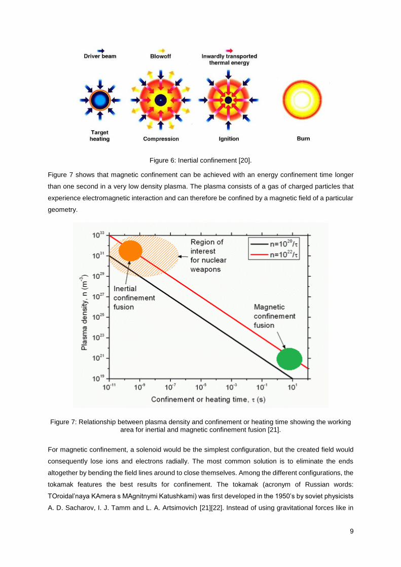
This process is illustrated by Figure 6.
9
Figure 6: Inertial confinement [20].
Figure 7 shows that magnetic confinement can be achieved with an energy confinement time longer
than one second in a very low density plasma. The plasma consists of a gas of charged particles that
experience electromagnetic interaction and can therefore be confined by a magnetic field of a particular
geometry.
Figure 7: Relationship between plasma density and confinement or heating time showing the working area for inertial and magnetic confinement fusion [21].
For magnetic confinement, a solenoid would be the simplest configuration, but the created field would
consequently lose ions and electrons radially. The most common solution is to eliminate the ends
altogether by bending the field lines around to close themselves. Among the different configurations, the
tokamak features the best results for confinement. The tokamak (acronym of Russian words:
TOroidal’naya KAmera s MAgnitnymi Katushkami) was first developed in the 1950’s by soviet physicists
A. D. Sacharov, I. J. Tamm and L. A. Artsimovich [21][22]. Instead of using gravitational forces like in

10
the stars, the use of magnetic fields, which confine the plasma in the torus chamber, as shown in Figure
8, allows to reach the appropriate conditions for fusion.
Figure 8: Tokamak coil system, magnetic and toroidal fields and the resulting plasma confinement [22].
From the point of view of the neutronics, which will be the main topic of this Thesis, the inertial
confinement features neutrons of 12 MeV, instead of the 14.1 MeV neutrons of high density plasmas.
The amount of energy created relies on particles colliding and fusing. The greater the density, the more
the particles collide and the higher the probability of fusion. The density reached in stellar interiors are
of the order of 1033 particles/m3 at a temperature of 3 x 10⁷ K, while metals have a density of
approximately 1028 – 1029 particles/m3 and air of 2.7 x 1025 molecules/m3 in standard conditions.
Gravitational confinement is therefore defined as a type of confinement occurring in the sun and the
stars whereby gravity holds the plasma nuclei close enough together to fuse [23].
The Lawson criterion provides the condition under which efficient production of fusion energy is possible.
Basically, it uses the electron density and the energy confinement time [24]. For the deuterium-
tritium reaction:
𝑛𝜏𝐸 ≥ 1.5× 10²⁰ 𝑠
𝑚3 (2.5)
Technologically, it is still necessary to prove the vast majority of the necessary technologies for a fusion
power plant.
2.2 Mechanisms of Nuclear Interaction
Nuclear interactions can be represented as
𝑎 + 𝑋 → 𝑌 + 𝑏, (2.6)

11
where a is the incoming particle or light element that acts as a projectile, X is the target nucleus, Y is
the resultant nucleus and b is the outgoing particle. It can be simplified in the form of X(a,b)Y [25]. Some
examples are:
𝐻𝑒 +24 𝑁 → 𝑂 + 𝐻1
18
177
14 (2.7)
𝑛 + 𝐵 → 𝐿𝑖 + 𝐻𝑒24
37
510
01 (2.8)
Every nuclear interaction must obey the following laws [26]:
Conservation of nucleons: the total number of nucleons before and after a nuclear reaction is
not changed;
Conservation of charge: the sum of the charges of all particles involved in the reaction before
and after must be preserved;
Conservation of linear and angular momentum: the total momentum of interacting particles
before and after the reaction is not changed;
Conservation of energy: energy, including the rest mass energies of particles, is not changed
by a nuclear reaction.
The energy of the reaction is represented as follows:
𝑄 = (𝑀𝑛 + 𝑀𝑥 − 𝑀𝑦 − 𝑀𝑏) ∗ 𝑐2 (2.9)
If 𝑄 > 0, the reaction is exothermic and some of the nuclear mass is converted into kinetic energy. If
𝑄 < 0, the reaction is endothermic and the kinetic energy is converted into mass and hence there is a
net decrease of the total kinetic energy of the particles. The velocity at which a 14.1 MeV neutron is
emitted in a fusion reaction is
𝑣 = √2 ∗ 𝐸
𝑀𝑛
≈ 52 ∗ 106𝑚/𝑠
(2.10)
2.2.1 NEUTRON INTERACTIONS WITH MATTER
Due to their lack of charge, neutrons cannot interact through Coulomb forces with charged particles,
and therefore they are not stopped in the ITER’s tokamak by electromagnetic forces. For that reason,
they travel much larger distances in the materials than protons or electrons. For instance, the mean free
path, which is the average distance travelled by a moving particle between successive collisions, of a
neutron of 2 MeV in water is 3.2 cm [27].
Neutrons can be separated mainly into three categories according to their energies: Thermal (E~0.025
eV), epithermal (0.025 eV <E<100 keV) and fast neutrons (E>100 keV) [28]. In addition to the energy
classification, the neutron can be characterized by its De Broglie wavelength, calculated as:
𝜆 =ℎ
𝑝=
ℎ
√2 ∗ 𝑚𝑛 ∗ 𝐸≅
2.86 ∗ 10−9
√𝐸(𝑒𝑉)(𝑐𝑚),
(2.11)

12
where ℎ is the Planck’s constant, 𝑝 is the momentum, and 𝑚𝑛 is the mass of the neutron. At decreasing
energies, optical properties such as refraction and reflection of neutrons predominate in ordinary matter.
As an example, for neutrons of 0.01 eV, the wavelength is approximately 10−8cm, the value of the
diameter of the atom; therefore these neutrons can be diffracted as X-rays do, but since they penetrate
further they are suited for bulk materials [29]. As the energy increases, it is more common to point out
neutrons as projectiles colliding with the individual particles that make up the nuclei. For fast neutrons
of 1 MeV, the wavelength is in the order of magnitude of 10−12cm, which is the magnitude of the diameter
of the nucleus [30].
In order to understand neutron interactions with matter, the term cross-section is necessary. Normally
measured in barns (10-24 cm2), the cross-section is the target area presented by a nucleus to an
approaching neutron, measured as area on a plane normal to the motion of the neutron. Put simply, it
is the area of projection of the actual nucleus on the plane, as shown in Figure 9 [31].
Figure 9: Neutron cross sections and rate of reaction, adapted from [30].
A more sophisticated definition for cross-section derives from the meaning of rate of nuclear reaction,
R, which is proportional to the intensity of the neutron beam I (neutrons/s.cm2) and the number of atoms
in the target per unit area N (atoms/ cm2). The constant of proportionality is known as the microscopic
cross-section 𝜎 and quantifies the probability of any type of interaction that characterizes a nuclear
reaction.
𝑅 = 𝑛 ∙ 𝑣 ∙ 𝑁 ∙ 𝜎 = 𝐼 ∙ 𝑁 ∙ 𝜎 (2.12)
The cross sections depend heavily on the kinetic energy of the incident neutrons [32]. Figure 10 shows
the variation of the cross section of U-238 with the energy of the neutron. There are three main regions
in the cross section plots. In the low-energy region, the cross sections vary approximately as 1/𝑣 , being

13
𝑣 the neutron speed [33]. Then there is the resonance region, where the cross sections exhibit a high
sensitivity to slight variations in the energy of the incoming neutron, and the unresolved resonance
region, where the resonances are so close to each other that they cannot be resolved [34]. In this specific
case, the cross section describes the probability of undergoing radiative capture, described hereafter.
Figure 10: Radiative capture cross-section of Uranium-238 (data obtained from [27]).
The macroscopic cross section characterizes the probability of the neutrons interacting with all the nuclei
of a material. It is the given by:
𝛴𝑡 = 𝑁 ∙ 𝜎𝑡 , (2.13)
where N is the atomic density of the material (atoms/cm3). It has units of cm-1. Unlike microscopic cross
sections, 𝛴𝑡 is used to define the probability of interaction in a macroscopic volume instead of a single
nucleus. The macroscopic cross section can be expressed as a function of the mean free path:
𝛴𝑡 = 1
𝜆 (𝑚𝑒𝑎𝑛 𝑓𝑟𝑒𝑒 𝑝𝑎𝑡ℎ)
(2.14)
Furthermore, it can be used to describe the intensity of a neutron beam hitting a material as a function
of the distance travelled in the material. Its intensity decreases with the distance according to the
following exponential attenuation law:
𝐼(𝑥) = 𝐼0 ∙ 𝑒−𝛴𝑥 (2.15)
Resonance
region
1/v region
Unresolved
resonance
region

14
The total cross sections, 𝜎𝑡 or 𝛴𝑡 , can be obtained from the sum of the individual cross sections of the
different interactions that a neutron can experience.
Neutrons are attenuated (reduced in energy and numbers) by two major types of interactions: scattering
and absorption. Table shows the different types of interactions of neutrons with matter:
Scattering Elastic (n,n)
Inelastic (n, n’ Ɣ)
Absorption Radiative capture (n, Ɣ)
Capture with emission of charged
particles (n,α);(n,p);(n,d)
Fission (n,f)
(n,2n), (n,3n), spallation, etc.
Table 2: Different mechanisms of neutron interaction, adapted from [30]
Scattering events have the effect of changing the speed and the direction of the neutron and can be
classified into elastic and inelastic scattering. In elastic scattering, represented in Figure 11, a neutron
interacts with a nucleus and bounces off. Some of the kinetic energy of the neutron is transmitted to the
nucleus of the atom, increasing its kinetic energy and slowing down the neutron. The incident neutron
does not necessarily have to “touch” the nucleus; it may be scattered by the short range nuclear forces
when it approaches close enough to the nucleus. This type of elastic scattering is called potential
scattering. It occurs with incident neutrons that have an energy of up to 1 MeV, approximately, and may
be modeled as a billiard ball collision between a neutron and a nucleus.
Figure 11: Potential elastic scattering, adapted from [32].
A more unusual type of elastic scattering is called compound elastic or resonance elastic scattering,
which occurs if the kinetic energy of an incident neutron is just right to form a resonance. Then, the
neutron may be absorbed, forming a relatively long-lived (~ > 10−17sec ) compound [35], but it is emitted
afterwards.

15
The formation of a compound nucleus can be represented as
𝑛01 + 𝑋𝑍
𝐴 → 𝑋𝑍𝐴+1 ∗ (2.16)
This is more common in inelastic collisions whereby the compound nucleus decays through the emission
of a neutron, but not necessarily the same neutron that hit the nucleus in the first place. Whereas in the
elastic scattering reaction the total kinetic energy and momentum of the system is conserved, in inelastic
scattering there is a loss of kinetic energy needed to produce an excited state of the nucleus, which
decays to the fundamental state through the emission of Ɣ radiation (see Figure 12). There is no
conservation of kinetic energy, as the variation of kinetic energy is used to leave the nucleus in the
excited state.
Figure 12: Inelastic scattering, adapted from [32].
If the mass of the nucleus is similar to the mass of the neutron, the neutron loses more energy than
when it collides with heavy nuclei. The average energy loss of a neutron undergoing elastic scattering
is:
𝐴𝑣𝑒𝑟𝑎𝑔𝑒 𝑒𝑛𝑒𝑟𝑔𝑦 𝑙𝑜𝑠𝑠 =2𝐸𝐴
(𝐴 + 1)2,
(2.17)
where E is the kinetic energy of the neutron and A is the atomic weight of the target nucleus [36].
Therefore, light materials attenuate neutrons more effectively. That is why they are used in fission
reactors as moderators in order to decrease the energy of the neutrons to be able to increase the cross
the probability of inducing fission. As an example, Table 3 shows the average number of collisions
required to reduce a neutron's energy from 2 MeV to 0.025eV through elastic scattering.
Element Atomic weight Number of collisions
Hydrogen 1 27
Deuterium 2 31
Helium 4 48

16
Beryllium 9 92
Carbon 12 119
Uranium 238 2175
Table 3: Average number of collisions required to reduce a neutron's energy from 2 MeV to 0.025eV through elastic scattering [36].
The energy loss in inelastic scattering depends on the energy levels within the nucleus. Inelastic
scattering is only possible when the neutron has sufficient energy to induce excited states in the nucleus.
In an absorption reaction, the neutron is absorbed into the nucleus of an atom. The nucleus may re-
arrange its internal structure through the emission of one or more gamma rays (radiative capture),
charged particles or one or more neutrons. If the nucleus emits only one neutron, then it is
indistinguishable from a scattering event. When the target nucleus is fissionable, a fission reaction may
occur, whereby the nucleus splits into two nuclei of intermediate masses (the mass of each nucleus is
variable), emitting a variable number of neutrons in the process.
Radiative capture occurs at most neutron energy levels, but it is more probable at lower energies [37].
The following reaction, represented in Figure 13, takes place:
𝑛01 + 𝑋𝑍
𝐴 → 𝑋𝑍𝐴+1 ∗ → 𝑋 + 𝛾𝑍
𝐴+1 (2.18)
A gamma photon is emitted and the target nucleus is changed to a different isotope of the same element.
Figure 13: Radiative capture, adapted from [38].
Transmutation, which is the transformation of one element into another through a nuclear reaction, may
occur when the compound nucleus emits a charged particle, as shown in Figure 14. An example of this
type of capture is the following:
𝑛 + 𝐵 →510 𝐿𝑖 + 𝛼3
7 (2.19)

17
Figure 14: Capture with emission of charged particles, adapted from [38]
The large absorption cross section of helium-3, uranium-235 and boron-10 for the production of charged
particles with low-speed neutrons makes it appropriate for use in neutron detectors. Since only thermal
neutrons are detected, most detectors feature moderators, such as hydrogen or deuterium. Note that
hydrogen requires fewer collisions than deuterium in order to moderate the neutron. Despite the cost
and the abundance of hydrogen or water, the use of deuterium can be used instead as it features a
smaller absorption cross section for neutrons. The high absorption cross sections of boron and cadmium
make them useful as thermal-neutron poisons [36].
When nuclear fission occurs, the compound nucleus formed with the absorption of a neutron is split into
two lighter nuclei (fission fragments) releasing gamma radiation as well as a variable number of
neutrons. An example of a fission reaction initiated by a thermal neutron is:
𝑛 + 𝑈 →92235 𝑈∗ → 𝐾𝑟36
89 + 𝐵𝑎 + 3𝑛56144
92236 (2.20)
Figure 15 shows graphically the mechanism of nuclear fission, whereby a neutron encounters a nucleus
and forms a compound nucleus. The compound nucleus then emits two fragments, gamma radiation
and two neutrons in order to de-energize. The fission products are highly radioactive and decay through
the emission of Ɣ and β radiation [34] .
Figure 15: Nuclear fission, adapted from [34].

18
2.2.2 PHOTON INTERACTIONS WITH MATTER
Electromagnetic radiation can be considered as a beam of photons with energy:
𝐸 = ℎ 𝜈 (2.21)
Photons are neutral particles so they do not interact by Coulomb forces. If the energy of the incident
photon is above 10 eV, then photons may undergo photoelectric and Compton effect and ionize matter
directly [39]. However, photons are called indirectly ionizing radiation since most of the affected atoms
in matter are ionized directly by the secondary beta particles, which come from the ejection of an
electron from an atom at relativistic speeds [40]. The interactions of photons with matter that lead to the
production of secondary beta particles are:
Photoelectric effect
Compton effect
Pair production
The probability of photon interaction with matter depends on the incident energy of the photon E and
the atomic number of the target Z.
Table 4 shows that the cross section for photoelectric effect is higher for low energies of the incident
photon and for heavy target nuclei. On the other hand, it is more probable for pair production to occur
at higher energies.
Mechanism Cross section (barns)
Photoelectric effect
σ = k 𝑍𝑛
𝐸3
n between 3 and 5 depending on the energy
of the photon
Compton effect
σ = k 𝑍
𝐸
Pair production
σ = k Z2 (𝐸 −1.022 MeV)
Table 4: Dependence of the total cross section on the incident energy of the photon and the atomic number according to the main different mechanisms [27].

19
Figure 16 describes the dependence of the cross section on the energy of the incident photon for the
case of lead, where τ is the photoelectric effect, σINCOH is the incoherent (Compton) scattering, σCOH is
the coherent scattering, Κn is the nuclear-field pair production, Κe is the electron-field production (triplet)
and σPH.N. is the nuclear photoabsorption. The different processes are explained hereafter.
Figure 16: Contributions of different effects to the total measured cross section in lead over the photon energy range between 10eV to 100 GeV [37].
The photoelectric effect is a process whereby a photon is absorbed by the atom it encounters. The
photon transmits all its energy to an atomic electron. This electron is called photoelectron and escapes
from the atom with a kinetic energy equal to the difference between the energy of incident photon and
the binding energy of the atom B, which in turn is dependent on the atomic layer at which the electron
is located:
𝐸𝑒 = ℎ 𝜈 − 𝐵 (2.22)
The Compton effect is equivalent to an inelastic collision, as part of the photon energy is transferred to
the electron and a less-energetic photon bounces off, which means that it has lower frequency (or longer
wavelength).
For a quantitative analysis, the laws of conservation of energy and momentum are used:
𝐸𝛾 + 𝑚𝑒 𝑐2 = 𝐸𝛾′ + 𝑚𝑒 𝑐
2 + 𝐸𝑒 + 𝐵 (2.23)
𝑝𝛾⃗⃗⃗⃗ = 𝑝𝛾′⃗⃗ ⃗⃗ ⃗ + 𝑝𝑒,⃗⃗ ⃗⃗ (2.24)
20
where 𝐸𝛾 is the energy of the incident photon, 𝐸𝛾′ is the energy of the scattered photon, 𝐸𝑒 is the kinetic
energy after the collision, B is the binding energy of the electron and 𝑚𝑒 𝑐2 is the energy equivalent to
the mass of the electron at rest.
If the electron is considered as a free electron, then B ≈ 0 and equation 2.25 can be simplified:
𝐸𝛾 = 𝐸𝛾′ + 𝐸𝑒 (2.25)
After some operations, the difference in wavelength after and before scattering is obtained:
∆𝜆 = λ’ − λ = λ𝑐 (1 − 𝑐𝑜𝑠𝜃), (2.26)
where λ’ is the wavelength of the scattered photon, λ is the wavelength of the incident photon and 𝜃 is
the angle formed between the scattered photon and the incident photon. Compton’s wavelength is
represented by λ𝑐 and its value is:
λ𝑐 =ℎ
𝑚𝑒𝑐= 2.43 ∗ 10−12 = 0.0243 Å
(2.27)
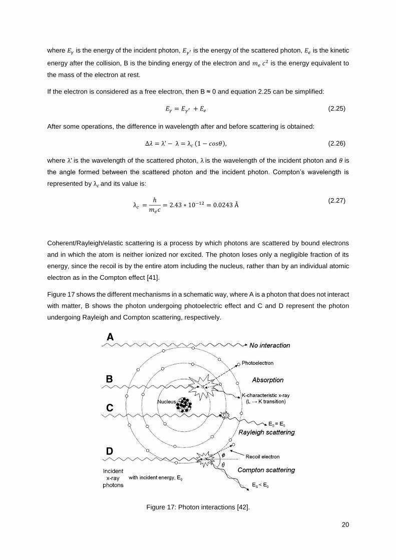
Coherent/Rayleigh/elastic scattering is a process by which photons are scattered by bound electrons
and in which the atom is neither ionized nor excited. The photon loses only a negligible fraction of its
energy, since the recoil is by the entire atom including the nucleus, rather than by an individual atomic
electron as in the Compton effect [41].
Figure 17 shows the different mechanisms in a schematic way, where A is a photon that does not interact
with matter, B shows the photon undergoing photoelectric effect and C and D represent the photon
undergoing Rayleigh and Compton scattering, respectively.
Figure 17: Photon interactions [42].
21
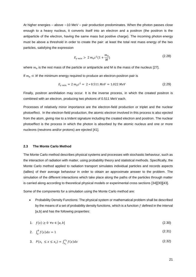
At higher energies – above ~10 MeV – pair production predominates. When the photon passes close
enough to a heavy nucleus, it converts itself into an electron and a positron (the positron is the
antiparticle of the electron, having the same mass but positive charge). The incoming photon energy
must be above a threshold in order to create the pair: at least the total rest mass energy of the two
particles, satisfying the expression
𝐸𝛾 𝑚𝑖𝑛 > 2 𝑚0𝑐2(1 +
𝑚0
𝑀) (2.28)
where 𝑚0 is the rest mass of the particle or antiparticle and M is the mass of the nucleus [27].
If 𝑚0 ≪ 𝑀 the minimum energy required to produce an electron-positron pair is
𝐸𝛾 𝑚𝑖𝑛 = 2 𝑚0𝑐2 = 2 ∗ 0.511 𝑀𝑒𝑉 = 1.022 𝑀𝑒𝑉 (2.29)
Finally, positron annihilation may occur. It is the inverse process, in which the created positron is
combined with an electron, producing two photons of 0.511 MeV each.
Processes of relatively minor importance are the electron-field production or triplet and the nuclear
photoeffect. In the electron-field production, the atomic electron involved in this process is also ejected
from the atom, giving rise to a trident signature including the created electron and positron. The nuclear
photoeffect is the process in which the photon is absorbed by the atomic nucleus and one or more
nucleons (neutrons and/or protons) are ejected [41].
2.3 The Monte Carlo Method
The Monte Carlo method describes physical systems and processes with stochastic behaviour, such as
the interaction of radiation with matter, using probability theory and statistical methods. Specifically, the
Monte Carlo method applied to radiation transport simulates individual particles and records aspects
(tallies) of their average behaviour in order to obtain an approximate answer to the problem. The
simulation of the different interactions which take place along the paths of the particles through matter
is carried along according to theoretical physical models or experimental cross sections [34][30][43].
Some of the components for a simulation using the Monte Carlo method are:
Probability Density Functions: The physical system or mathematical problem shall be described
by the means of a set of probability density functions, which is a function 𝑓 defined in the interval
[a,b] and has the following properties:
1. 𝑓(𝑥) ≥ 0 ∀𝑥 ∈ [𝑎, 𝑏] (2.30)
2. ∫ 𝑓(𝑥)𝑑𝑥 = 1𝑏
𝑎 (2.31)
3. 𝑃(𝑥1 ≤ 𝑥 ≤ 𝑥2) = ∫ 𝑓(𝑥)𝑑𝑥𝑥2
𝑥1 (2.32)

22
Pseudo-random number generator: A source of pseudo-random numbers from a probability
density function uniformly distributed between 0 and 1 is needed [44][45]. Even though pseudo-
random number generators still exhibit periodicity (when a number is repeated the whole
sequence is repeated), they feature sophisticated and efficient algorithms generated from an
initial number, called the seed. The seed can be changed to produce different random number
sequences. For example, when the pseudo-random generator is called, the seed can be
extracted from the computer system clock.
Error estimate: The error is proportional to 1/√𝑁, where N is the number of histories and is
inversely proportional to the computational time.
The name Monte Carlo arose from the analogy between the statistical sampling process based on the
selection of random numbers with throwing dice in the gambling casino of the capital of Monaco. Due
to increased computational capacity and need to solve problems of diffusion of neutrons, the Monte
Carlo method became more relevant during the II World War. Nowadays, there are several radiation
transport programs that use this method, such as [46]:
EGSnrc and PENELOPE, appropriate for electron, positron and photon transport;
GEANT4 and FLUKA, which can also simulate neutrons and many more types of particles;
MARS, for thermal and stress analyses;
PHITS and SHIELD, focused on the analysis of heavy ions;
TRIM, for protons and heavy ions undergoing Coulomb interactions.
Monte Carlo N-Particle (MCNP) is another radiation transport program that applies the Monte Carlo
method, developed by the National Laboratory Los Alamos in the United States. It is used to simulate
neutron, photon and electron transport in arbitrary three-dimensional geometries. Furthermore, MCNP6
uses ENDF1 formatted data such as the FENDL (Fusion Evaluated Nuclear Data Library) libraries.
These libraries feature point-wise cross section data for neutron transport, which means that there is no
approximation or averaging in the cross section data. A very accurate description of neutron transport
is thus attained [47].
The transport of a single particle can be described as a sequence of collisions, events, occurring at
discrete spatial locations followed by the transition of the particle from one collision point to the next
collision point. At collisions, the incoming particle direction and energy are changed, whereas during the
transition between two consecutive collision points the energy and direction of the particle is maintained.
At first, MCNP creates a virtual particle according to the source specification written by the user: the
energy, direction and starting position are specified. The distance to the next collision is sampled from
𝑙 = −1
𝛴𝑎
ln(𝜉) (2.33)
where 𝑙 is the distance to next collision in cm, 𝛴𝑎 is the total macroscopic cross section in cm-1 and 𝜉 is
a uniformly distributed random number between 0 and 1 [47]. Knowing the fractional composition of

23
each nuclide for a given material, MCNP uses the pseudo-random generator to determine all required
physical parameters during the “life” of the particle (also called the history of the particle), such as: with
which nuclide the particle will interact, the type of interaction the particle and the nuclide undergo
(depending on the cross sections) and the direction and energy of emission of secondary particles.
Figure 18 shows how the history of a neutron is simulated in MCNP. The steps that the neutron follows
during this history are the following:
1. In the first event, the neutron undergoes inelastic scattering. MCNP follows the path of the
neutron first and then focuses on the secondary particles created. In other words, the photon
created in this case is temporarily stored in memory until the neutron is “killed”. The neutron is
deflected through an angle determined from the scattering distribution which is stored in the
nuclear data.
2. Then the neutron is absorbed. Concretely, the neutron undergoes an (n,2n) reaction. So the
code creates two neutrons with particular energies and directions.
3. Neutron absorption takes place for one of the neutrons from the previous (n,2n) reaction.
4. The second neutron produced in the (n,2n) reaction is retrieved from memory and leaks from
the system.
5. The photon produced in the inelastic scattering reaction is retrieved from memory and
undergoes pair production.
6. Photon absorption takes place for one of the photons that are produced.
7. The other photon which is retrieved from memory and was created from the pair production
reaction undergoes a scattering reaction.
8. The photon leaks from the system.
Figure 18: Neutron interaction events in MCNP [48].
24
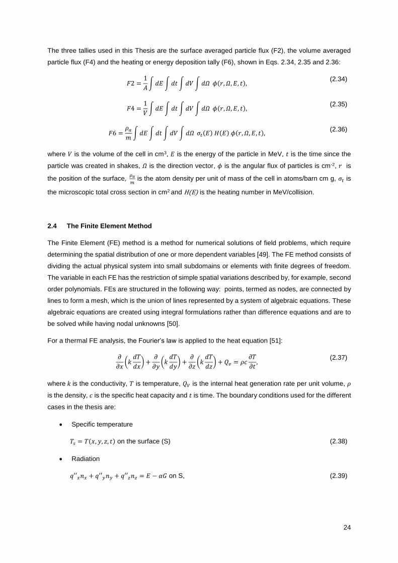
The three tallies used in this Thesis are the surface averaged particle flux (F2), the volume averaged
particle flux (F4) and the heating or energy deposition tally (F6), shown in Eqs. 2.34, 2.35 and 2.36:
𝐹2 =1
𝐴∫𝑑𝐸 ∫𝑑𝑡 ∫𝑑𝑉 ∫𝑑𝛺 𝜙(𝑟, 𝛺, 𝐸, 𝑡),
(2.34)
𝐹4 =1
𝑉∫𝑑𝐸 ∫𝑑𝑡 ∫𝑑𝑉 ∫𝑑𝛺 𝜙(𝑟, 𝛺, 𝐸, 𝑡),
(2.35)
𝐹6 =𝜌𝑎
𝑚∫𝑑𝐸 ∫𝑑𝑡 ∫𝑑𝑉 ∫𝑑𝛺 𝜎𝑡(𝐸) 𝐻(𝐸) 𝜙(𝑟, 𝛺, 𝐸, 𝑡),
(2.36)
where 𝑉 is the volume of the cell in cm3, 𝐸 is the energy of the particle in MeV, 𝑡 is the time since the
particle was created in shakes, 𝛺 is the direction vector, 𝜙 is the angular flux of particles is cm-2, 𝑟 is
the position of the surface, 𝜌𝑎
𝑚 is the atom density per unit of mass of the cell in atoms/barn cm g, 𝜎𝑡 is
the microscopic total cross section in cm2 and H(E) is the heating number in MeV/collision.
2.4 The Finite Element Method
The Finite Element (FE) method is a method for numerical solutions of field problems, which require
determining the spatial distribution of one or more dependent variables [49]. The FE method consists of
dividing the actual physical system into small subdomains or elements with finite degrees of freedom.
The variable in each FE has the restriction of simple spatial variations described by, for example, second
order polynomials. FEs are structured in the following way: points, termed as nodes, are connected by
lines to form a mesh, which is the union of lines represented by a system of algebraic equations. These
algebraic equations are created using integral formulations rather than difference equations and are to
be solved while having nodal unknowns [50].
For a thermal FE analysis, the Fourier’s law is applied to the heat equation [51]:
𝜕
𝜕𝑥(𝑘
𝑑𝑇
𝑑𝑥) +
𝜕
𝜕𝑦(𝑘
𝑑𝑇
𝑑𝑦) +
𝜕
𝜕𝑧(𝑘
𝑑𝑇
𝑑𝑧) + 𝑄𝑣 = 𝜌𝑐
𝜕𝑇
𝜕𝑡,
(2.37)
where 𝑘 is the conductivity, 𝑇 is temperature, 𝑄𝑉 is the internal heat generation rate per unit volume, 𝜌
is the density, 𝑐 is the specific heat capacity and 𝑡 is time. The boundary conditions used for the different
cases in the thesis are:
Specific temperature
𝑇𝑠 = 𝑇(𝑥, 𝑦, 𝑧, 𝑡) on the surface (S) (2.38)
Radiation
𝑞′′𝑥𝑛𝑥 + 𝑞′′𝑦𝑛𝑦 + 𝑞′′𝑧𝑛𝑧 = 𝐸 − 𝛼𝐺 on S, (2.39)

25
where 𝑞′′𝑥, 𝑞′′
𝑦 and 𝑞′′
𝑧 are components of heat flow per unit area, 𝑛𝑥, 𝑛𝑦, and 𝑛𝑧 are the components
of the normal unit vector to the surface, 𝛼 is the absorptivity, G is the incoming heat flow per unit area
named irradiation and E is the emissive power which is expressed by:
𝐸 = 𝜀𝜎𝑇4, (2.40)
where 𝜀 is the emissivity and 𝜎 is the Stefan-Boltzmann constant.
Steady-state regime:
𝜕𝑇
𝜕𝑡= 0
(2.41)
Eq. 2.37 can be rewritten as follows after applying Fourier’s Law, the Galerkin weighted residual method
[52] and the divergence theorem [53] to the components of the heat flow per unit area:
∫ 𝜌𝑐𝜕𝑇
𝜕𝑡𝑁𝑖𝑑𝑉
𝑉
− ∫ [𝜕𝑁𝑖
𝜕𝑥 𝜕𝑁𝑖
𝜕𝑦 𝜕𝑁𝑖
𝜕𝑧] {𝑞}𝑑𝑉
𝑉
= ∫ 𝑄𝑣𝑁𝑖𝑑𝑉
𝑉
+ ∫{𝑘[𝐵]{𝑇}}𝑇{𝑛}
𝑆
𝑁𝑖𝑑𝑆 − ∫(𝜀𝜎𝑇4 − 𝛼𝐺)
𝑆
𝑁𝑖𝑑𝑆
(2.42)
where {𝑛} is the outer normal to the surface of the body and [B] is the matrix containing the partial
derivatives of the shape functions 𝑁𝑖, which are used for interpolation of temperature inside a FE.
Boundary conditions (2.38) and (2.39) are inserted. Note that as vacuum in the vessel is present,
convection is neglected.
Hence, Eq. 2.42 after assembly becomes:
[𝐶]{�̇�} + ([𝐾𝑐] + [𝐾𝑟𝑎𝑑]){𝑇} = {𝑅𝑇} + {𝑅𝑟𝑎𝑑} + {𝑅𝑄𝑣}, (2.43)
where [𝐶] is the general global specific heat, ([𝐾𝑐] + [𝐾𝑟𝑎𝑑]) are the conductivity matrices, and ({𝑅𝑇} +
{𝑅𝑄} + {𝑅𝑟}) are vectors for the global heat flux, radiation and heat generation, respectively, expressed
as:
[𝐶] = ∫ 𝜌𝑐 [𝑁]𝑇[𝑁]𝑑𝑉
𝑉
[𝐾𝑐] = ∫ 𝑘 [𝐵]𝑇[𝐵]𝑑𝑉
𝑉
[𝐾𝑟𝑎𝑑] = ∫ 𝜀𝜎𝑇4[𝑁]𝑑𝑆
𝑆

26
[𝑅𝐵] = ∫{𝑘[𝐵]{𝑇}}𝑇{𝑛}[𝑁]𝑇𝑑𝑆
𝑆
[𝑅𝑟𝑎𝑑] = −∫ 𝛼𝐺[𝑁]𝑇𝑑𝑆
𝑆
[𝑅𝑄𝑣] = ∫ 𝑄𝑣[𝑁]𝑇𝑑𝑉
𝑉
(2.44)
For a steady rate analysis, the governing equation after applying Eq. 2.41 is:
([𝐾𝑐] + [𝐾𝑟𝑎𝑑]){𝑇} = {𝑅𝑇} + {𝑅𝑟𝑎𝑑} + {𝑅𝑄𝑣} (2.45)
This formulation is adopted in the FE analysis conducted in this thesis.
27
3 METHODOLOGY
3.1 Shielding Sphere
3.1.1 MCNP PROCEDURE
A simplification of the real problem in ITER is done for practical and training purposes to deepen the
knowledge about shielding materials. The shielding sphere shows the procedure to obtain the power
density by using the Monte Carlo method in MCNP6 and the temperature distribution by using the Finite
Element method in ANSYS. In this case, water and lead will be the selected shielding materials for the
homogeneous source of 14 MeV neutrons. Moreover, they serve as a model for the innovative interface
MMA.
At first, a sphere of radius 400 cm (cell 1) is defined as an approximation of the radius size of the plasma
(neutron source). Cell cards indicate the cell number followed by the material number and the density
among other information. The mass density of the cell starts with a negative sign to indicate that it is in
g/cm3. No density is entered for a void cell (written as 0 after the cell number). In the case of lead, the
density is 11.34 g/cm3 while water has a density of 1 g/cm3. The cells are the areas defined by the
surfaces that are shown in the next section.
1 0 -1 $source
2 1 -11.34 1 -2 $8 shielding layers
3 1 -11.34 2 -3
4 1 -11.34 3 -4
5 1 -11.34 4 -5
6 1 -11.34 5 -6
7 1 -11.34 6 -7
8 1 -11.34 7 -8
9 1 -11.34 8 -9
10 1 -11.34 9 -10
11 2 -1 -11 $water sphere
12 0 11 10 -12 $cell around the water sphere
13 0 12 $outer space
The surfaces are concentric spheres of different radii centred in the origin (So). The shielding layers
(cells) have a width of 40 cm and from surface 6 outwards they have a width of 75 cm.
C Surface cards
1 So 400 $sphere source
2 So 440 $shielding layers
3 So 480
4 So 520
5 So 560
6 So 600
7 So 675
8 So 725
9 So 800
10 So 875
28
11 SZ 885 10
12 So 1000
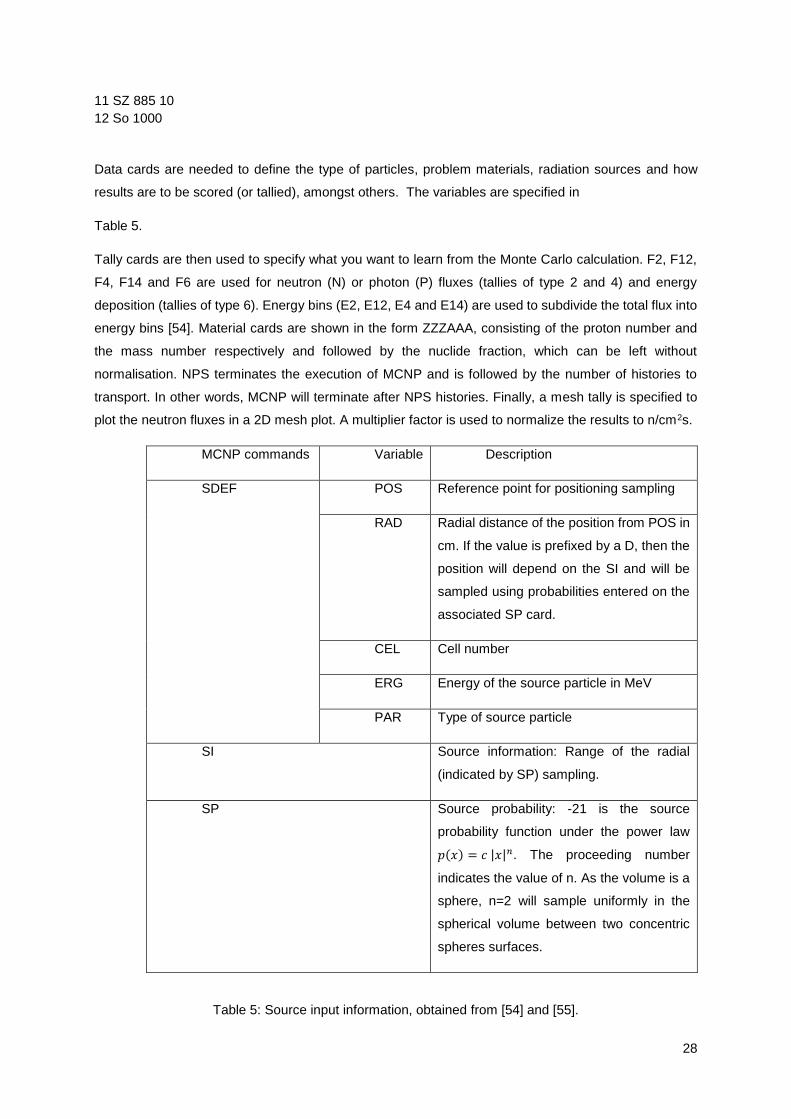
Data cards are needed to define the type of particles, problem materials, radiation sources and how
results are to be scored (or tallied), amongst others. The variables are specified in
Table 5.
Tally cards are then used to specify what you want to learn from the Monte Carlo calculation. F2, F12,
F4, F14 and F6 are used for neutron (N) or photon (P) fluxes (tallies of type 2 and 4) and energy
deposition (tallies of type 6). Energy bins (E2, E12, E4 and E14) are used to subdivide the total flux into
energy bins [54]. Material cards are shown in the form ZZZAAA, consisting of the proton number and
the mass number respectively and followed by the nuclide fraction, which can be left without
normalisation. NPS terminates the execution of MCNP and is followed by the number of histories to
transport. In other words, MCNP will terminate after NPS histories. Finally, a mesh tally is specified to
plot the neutron fluxes in a 2D mesh plot. A multiplier factor is used to normalize the results to n/cm2s.
MCNP commands Variable Description
SDEF POS Reference point for positioning sampling
RAD Radial distance of the position from POS in
cm. If the value is prefixed by a D, then the
position will depend on the SI and will be
sampled using probabilities entered on the
associated SP card.
CEL Cell number
ERG Energy of the source particle in MeV
PAR Type of source particle
SI Source information: Range of the radial
(indicated by SP) sampling.
SP Source probability: -21 is the source
probability function under the power law
𝑝(𝑥) = 𝑐 |𝑥|𝑛. The proceeding number
indicates the value of n. As the volume is a
sphere, n=2 will sample uniformly in the
spherical volume between two concentric
spheres surfaces.
Table 5: Source input information, obtained from [54] and [55].

29
C Data cards
mode n p
IMP:N 1 1 1 1 1 1 1 1 1 1 1 1 0
SDEF pos=0 0 0 rad=d1 cel=1 erg=14 par=N
SI1 0 400 $ radial sampling range: 0 to Rmax
SP1 -21 2 $ weighting for radial sampling: here r^2
F2:N 2 3 4 5 6 7 8 9 10 $average neutron fluxes across each shielding surface
E2 1e-5 100log 20 $from 10 eV to 20 MeV takes log spacing
F12:P 2 3 4 5 6 7 8 9 10
E12 1e-3 100log 20
F4:N 11 $neutron flux across the water sphere cell
E4 1e-5 100log 20
F14:P 11
E14 1e-3 100log 20 $Energy photons
F6:N,P 2 3 4 5 6 7 8 9 10 $Energy deposition across each shielding cell
M1 82000 1 $Natural lead
M2 1001 2 8016 1 $Water
NPS 1000000
tmesh
rmesh31:n FLUX
cora31 -1000 99i 1000
corb31 -400 4i 400
corc31 -1000 99i 1000
endmd
fm31 1.97e19
3.1.2 TRANSITION TO ANSYS
For the thermal analysis, the same geometry applied to MCNP6 is created with SolidWorks. First, half
a sphere of 420 cm radius is modelled. The piece is then extruded with a smaller sphere of 400 cm
radius, as shown in Figure 19.
The operation is repeated for all the outer semi-spheres. Finally, the ensemble of the pieces was made.
Figure 20 shows two pieces of different width picked from the final semi-sphere.
The geometry is used as input in ANSYS and a superficial temperature and the internal heat generation
in W/m3 obtained from MCNP6 were applied as boundary conditions.

30
Figure 19: Half a hollow sphere in SolidWorks.
Figure 20: Ensemble of pieces created in SolidWorks.
31
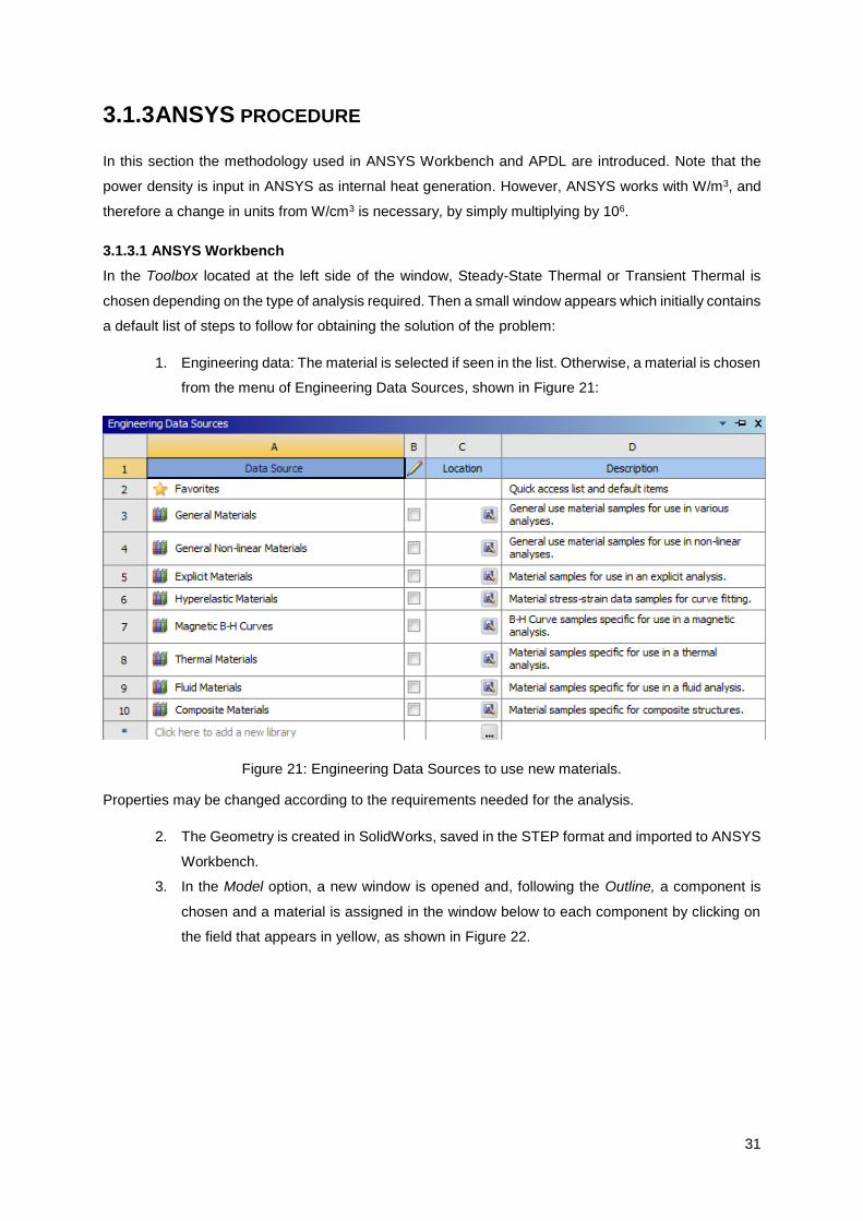
3.1.3 ANSYS PROCEDURE
In this section the methodology used in ANSYS Workbench and APDL are introduced. Note that the
power density is input in ANSYS as internal heat generation. However, ANSYS works with W/m3, and
therefore a change in units from W/cm3 is necessary, by simply multiplying by 106.
3.1.3.1 ANSYS Workbench
In the Toolbox located at the left side of the window, Steady-State Thermal or Transient Thermal is
chosen depending on the type of analysis required. Then a small window appears which initially contains
a default list of steps to follow for obtaining the solution of the problem:
1. Engineering data: The material is selected if seen in the list. Otherwise, a material is chosen
from the menu of Engineering Data Sources, shown in Figure 21:
Figure 21: Engineering Data Sources to use new materials.
Properties may be changed according to the requirements needed for the analysis.
2. The Geometry is created in SolidWorks, saved in the STEP format and imported to ANSYS
Workbench.
3. In the Model option, a new window is opened and, following the Outline, a component is
chosen and a material is assigned in the window below to each component by clicking on
the field that appears in yellow, as shown in Figure 22.

32
Figure 22: Assignment of the material to the component of the model.
After finishing with the geometry, the system is to be meshed as shown in Figure 23.
Figure 23: Mesh option in Outline list.
4. On top of the outline list, boundary conditions such as temperature at the surface and
internal heat generation are selected and applied to each of the bodies.
5. The solution of the thermal analysis is finally achieved.
3.1.3.2 ANSYS APDL
Another way of obtaining similar results is by using the APDL. Even though different skills are required,
the advantage is that it reduces the time needed to parametrize the FE model and performed the FE
analyses. Figure 24 shows the main steps that were followed:

33
Figure 24: Main menu in APDL.
1. In Preferences there are options for thermal, structural, ANSYS fluid and electromagnetic
analysis. Thermal analysis is selected.
2. In Preprocessor, the steps followed were:
a. Select the FE
b. In Material Props:
i. Checking the units.
ii. Selecting the material models and adding a model for each component.
iii. Assigning a value for the thermal properties, which are known and available in
the list presented in Figure 25.
Figure 25: Material models window.
c. Creating a model. Some available operations are: extrude, add and overlap areas.
d. Meshing:
i. Picked volumes are selected and for each volume an element type is attributed.
ii. In the MeshTool, the size of the mesh can be altered and all the volumes are
selected and meshed.

34
e. If needed, in Numbering Ctrls, nodes can be merged.
f. Applying boundary conditions (Loads).
3. Under the option of Solution, Solve is clicked.
4. In Postprocessor, results were read and plotted.
The code for these steps can be introduced in the main bar and can be obtained by clicking on File >List
> Log File.
3.1.4 MMA INTERFACE
A MATLAB-MCNP6-ANSYS interface was implemented to automatically input data such as: conductivity
and density of the material, composition of the shielding material, source intensity and temperature in
the outer layer. The aim of the interface is to be able to obtain the distribution temperature (i.e. maximum
temperature) of the shielding sphere automatically, i.e. without changing the MCNP6 and ANSYS input
files by hand. In this way, it is possible to perform a thermal analyses of a neutron source surrounded
by different shielding materials.
Annex I shows the MCNP6 code used for the shielding sphere. Cell cards include the definition of the
source and the eight shielding layers are rewritten in MATLAB code (annex III), introducing the density
of the material used as shielding. Surface and data cards are also used from the MCNP6 shielding
sphere bearing in mind the modifications needed for the multiplier factors in order to normalise results
for the F4 and F6 tallies. The material card is then defined as ZZZAAA 1, where ZZZ is the proton
number, AAA is 000, standing for the natural isotopic composition of the element, and 1 is the nuclide
fraction.
With the MATLAB code, MCNP6 runs and particular lines of the output file (‘run_o’) are read and used
as input data for ANSYS. Specifically, the lines are values of heat generation due to neutron irradiation,
which is known as power density (in W/m3) in MCNP6. The input data is completed by introducing the
variables of conductivity and density of the material, and the temperature in the outer layer as a boundary
condition. Annex II shows the two methods of implementing the problem (manually or in batch mode).
3.2 PPR
3.2.1 PRELIMINARY WORK
Figure 26 shows a plane (y=0) of the reference MCNP model provided by F4E before the beginning of
this work. This reference model, an effort of several institutions worldwide coordinated by the ITER
Organization (IO), is extremely detailed, featuring more than 350 000 lines of MCNP code. Making
changes to this model is therefore a difficult task, mainly due to the time it takes to visualize a plane in

35
the MCNP geometry plotter. Additionally, the location of gap 4 is particularly challenging, since it is tilted
in the x, y and z directions, and the MCNP plotter only allows the visualization of 2D geometries.
Figure 26: Sectional cut of the MCNP reference model (y=0) [11].
Figure 27 shows the location of gap 4 in the reference model before the PPR components were created
and implemented. It is clearly seen that there was space reserved in the model for the insertion of the
PPR components. The reference model was modified as required to introduce some additional features,
Location of the
PPR System

36
such as the cut-outs in the blanket modules to accommodate the antenna assembly and provide access
to the plasma [11].
Figure 27: Zoom for location of gap 4 in the MCNP reference model (plane defined by basis vectors (706.2, 240.3, 0.0) and (0.0, 0.0, 1.0)) [11].
To produce the new MCNP to be used in the nuclear analysis of the PPR in-vessel components of gap
4, the CAD models of gap 4 available in ITER’s ENOVIA database (where all the ITER CAD models are
stored) were converted into a simplified neutronics CAD model. The simplifications involved the removal
of spline surfaces, fillets and screws while preserving approximately the same volumes and masses of
the components. The simplified neutronics CAD model was then divided into separate cells. As they are
closer to the plasma, the parts of the antennas were divided into smaller cells (see Figure 28), which
allows a more detailed calculation in the elements exposed to higher radiation doses. Finally, the
simplified neutron CAD model was converted to the STEP format in order to be edited in ANSYS
SpaceClaim and converted in the CAD based modelling program MCAM [56] to the MCNP input format
[11].
Figure 28: In-vessel components of the PPR system. Left: Simplified neutronics CAD model. Right: Detail of the simplified neutronics CAD model [11].
1 2
3 4
5 67 8
133409
133410
133411
133412
133413
133414
133401133414
133415
133416
133417
133418
13341912231 12230
displacement

37
The result of the integration of the PPR in-vessel components of gap 4 into the MCNP reference model
provided by IO is represented in Figure 29. Apart from the insertion of the antennas and waveguides, a
cut was introduced in the top of blanket module #12, so that the antennas are facing the plasma directly
[11]. The model thus created was employed in this Thesis to perform the Monte Carlo simulations of the
system. The heat loads had in the system had already been calculated; they are reproduced in this work
and complemented with neutron and photon flux calculations, which are later used (the neutron fluxes)
to estimate the DPAs in all the elements of the system.
Figure 29 - Sectional cut of the final MCNP model, featuring the PPR components of gap 4.
3.2.2 MCNP PROCEDURE
The volumes and masses of each element of the PPR system, retrieved from the CAD models, are
shown in Table 6 (it is important to notice that cell 12230 features a higher mass than is apparent in
Figure 28, as it extends beyond what is shown in the Figure). The differences in volume of the CAD
models (from the model available in the ITER database to the simplified model), were kept below 0.1%
up to cell number 133414. For the remaining cells, the cross sectional surface area of the waveguides
was kept unchanged between the two CAD models while differences in volume are not possible to
compare as significant changes were done to the models.
From the input file, it has been checked that the mass density of the material used for all the cells of the
PPR system, which is SS316L(N)-IG, is 7.93 g/cm3, indicated by a negative sign for mass density in the
cell cards.
cut in the blanket

38
Cell
Number
Volume
(cm3)
Mass
(g)
133401 2.46 19.49
133402 2.46 19.49
133403 2.33 18.51
133404 2.33 18.51
133405 2.21 17.54
133406 2.21 17.54
133407 1.45 11.49
133408 1.45 11.49
133409 32.80 260.08
133410 161.15 1277.88
133411 184.52 1463.24
133412 178.24 1413.42
133413 474.59 3768.50
133414 30.49 241.80
133415 12.62 100.05
133416 12.62 100.05
133417 148.29 1175.95
133418 161.85 1283.49
133419 25.34 200.95
12230 1343.91 10657.20
12231 208.61 1654.25
Table 6: Cell numbers, volumes and masses of the PPR components of gap 4.
The F6 tally (or any number ended in 6) calculates the energy deposition in MeV/g∙source particle. As
neutrons and photons deposit both its energy in the cells, the F6 tally is followed by “N,P”, N standing
for neutrons and P for photons. In order to calculate the energy deposition, an SD card is used after the
F6 tally to input the masses (see Eq. 2.36). It is important to note that when the SD card is used after
the F4 tally it inputs volumes (instead of masses), necessary to calculate the particle fluxes across the
cells (see Eq. 2.35).
Then a multiplier factor is written in the code in order to output normalised results. Particularly, FM6 will
make the F6 tally output power per unit mass in W/g as it follows:
𝐹𝑀6 = 𝐸𝑛𝑒𝑟𝑔𝑦 𝑑𝑒𝑝𝑜𝑠𝑖𝑡𝑖𝑜𝑛 (
𝑀𝑒𝑉
𝑔 𝑠𝑜𝑢𝑟𝑐𝑒 𝑝𝑎𝑟𝑡𝑖𝑐𝑙𝑒) ∗ 1.60217662𝑥10−13 (
𝐽
𝑀𝑒𝑉)
∗ 𝑆𝑜𝑢𝑟𝑐𝑒 𝑖𝑛𝑡𝑒𝑛𝑠𝑖𝑡𝑦 (𝑠𝑜𝑢𝑟𝑐𝑒 𝑝𝑎𝑟𝑡𝑖𝑐𝑙𝑒
𝑠)
= 𝐸𝑛𝑒𝑟𝑔𝑦 𝑑𝑒𝑝𝑜𝑠𝑖𝑡𝑖𝑜𝑛 ∗ 1.60217662𝑥10−13 ∗ 1.973𝑥1019
= 3.1611𝑥106 (𝑊
𝑔),
(3.1)
Where the source intensity is obtained by knowing that 80% of the energy released in ITER is carried
by the neutrons and that the MCNP model features only a 40-degree sector of the tokamak (a factor of
40/360 is applied)

39
𝑆𝑜𝑢𝑟𝑐𝑒 𝑖𝑛𝑡𝑒𝑛𝑠𝑖𝑡𝑦 (
𝑛
𝑠) =
0.80 ∙ 500 (𝑀𝑊)
1.60217662𝑥10−13 (𝐽
𝑀𝑒𝑉) ∙ 14.1 (𝑀𝑒𝑉) ∙
40360
(3.2)
The following code shows how the nuclear heat loads were calculated:
F6:N,P 133401 133402 133403 133404 133405 133406 133407
133408 133409 133410 133411 133412 133413 133414
133415 133416 133417 133418 133419 12230 12231
SD6 19.49 19.49 18.51 18.51 17.54 17.54 11.49 11.49
260.08 1277.88 1463.24 1413.42 3763.50 241.80
100.05 100.05 1175.95 1283.49 200.95
10657.20 1654.25 $ masses
FM6 3.1611E+06
Another tally is used to show the neutron contribution and hence the photon contribution to the total
nuclear heat load (energy deposition).
F16:N 133401 133402 133403 133404 133405 133406 133407
133408 133409 133410 133411 133412 133413 133414
133415 133416 133417 133418 133419 12230 12231
SD16 19.49 19.49 18.51 18.51 17.54 17.54 11.49 11.49
260.08 1277.88 1463.24 1413.42 3763.50 241.80
100.05 100.05 1175.95 1283.49 200.95
10657.20 1654.25 $ masses
FM16 3.1611E+06
The F4:N and F14:P tallies calculate the neutron and photon fluxes across the same cells that were
input in the F6 tallies. An energy (En) is used to subdivide the flux into energy bins [54].
F4:N 133401 133402 133403 133404 133405 133406 133407
133408 133409 133410 133411 133412 133413 133414
133415 133416 133417 133418 133419 12230 12231
E4 1.00E-11 1.00E-10 1.00E-09 1.00E-08 1.00E-07 1.00E-06
2.00E-06 5.00E-06 1.00E-05 2.00E-05 5.00E-05 1.00E-04
2.00E-04 5.00E-04 1.00E-03 2.00E-03 5.00E-03 1.00E-02
2.00E-02 5.00E-02 1.00E-01 2.00E-01 5.00E-01 1.00E+00
1.20E+00 1.40E+00 1.60E+00 1.80E+00 2.00E+00 2.50E+00
3.00E+00 3.50E+00 4.00E+00 4.50E+00 5.00E+00 6.00E+00
7.00E+00 8.00E+00 9.00E+00 1.00E+01 1.10E+01 1.20E+01
1.30E+01 1.40E+01 1.50E+01 1.60E+01 1.71E+01 1.82E+01
1.92E+01 2.00E+01 2.50E+01 3.00E+01 3.50E+01 4.00E+01
4.50E+01 5.00E+01 5.50E+01 6.00E+01 6.50E+01 7.00E+01
7.50E+01 8.00E+01 8.50E+01 9.00E+01 9.50E+01 1.00E+02
1.06E+02 1.10E+02 1.16E+02 1.20E+02 1.26E+02 1.30E+02
1.36E+02 1.40E+02 1.46E+02 1.50E+02
SD4 2.46 2.46 2.33 2.33 2.21 2.21 1.45 1.45
32.80 161.15 184.52 178.24 474.59 30.49
12.62 12.62 148.29 161.85 25.34
1343.91 208.61

40
Finally, F14:P, E14 and SD14 are written afterwards in the code. The parameters take the same
values as F4:N, E4 and SD4.
The power per unit mass from MCNP6 is then multiplied by the density, which is 7.93 g/cm3, in order to
obtain the power density or total heat load (W/cm3), which will be used as input to calculate the
temperature distribution using ANSYS. The neutron flux spectra obtained in MCNP6 are then used to
calculate the DPAs. Figure 30 is a flow chart indicating the basic steps followed.
Figure 30: Flow chart showing the followed procedure. Left: MCNP6 outputs using the listed commands in the arrows. Right: Variables obtained.
In order to have meaningful results, the statistical errors of the Monte Carlo simulations were kept below
10%. This value was taken from the guidelines provided in the MCNP manual [43] for interpreting the
quality of the simulation results, represented in Table 7.
Error Quality
0.5 to 1.0 Not meaningful
0.2 to 0.5 Factor of a few
0.1 to 0.2 Questionable
< 0.10 Generally reliable
< 0.05 Generally reliable for point
detectors
Table 7: Guidelines for interpreting the statistical errors of the simulations [43].
In order to obtain statistical errors below 10%, 1E9 source particles were simulated in each run (nps
1E9).

41
3.2.3 NJOY PROCEDURE
The NJOY Nuclear Data Processing System is a computer code used for converting evaluated nuclear
data in the ENDF format into libraries for several practical applications. ENDF "tapes" are subdivided
internally into "materials" (MAT), "files" (MF), and "sections" (MT) [57].
When performing DPA calculations in ITER nuclear analyses the use of the latest version of the Fusion
Evaluated Nuclear Data Library (FENDL) is mandatory and it is recommended that natural iron is used
as an approximation instead of stainless steel. Cross sections for natural iron were thus applied instead
of using the material of the PPR, which is SS316L (N)-IG, due to unknown cross sections for some
elements such as Sn.
The different isotopes of natural iron in FENDL were identified with the following four numbers (MAT):
2625 for Fe54
2631 for Fe56
2634 for Fe57
2637 for Fe58
Once stored as libraries, input files were created according to the following modules:
Moder is the module which converts ENDF “tapes” back and forth between ASCII format and
the special NJOY blocked-binary format. Positive unit numbers refer to formatted tapes, and
negative unit numbers refer to blocked binary tapes with absolute magnitudes, normally in the
range 20-99.
Reconr reconstructs pointwise (energy-dependent) cross sections from ENDF resonance
parameters and interpolation schemes. Card 1 in reconr comprises of the first output unit, -21
for the ENDF tape, and the second output unit, -22 assigned for the PENDF tape. Card 2 is the
name for the PENDF tape. In this case, it is called ‘material 2625 library’. Then, card 3 indicates
the material to be reconstructed (MAT), followed by the number of cards of descriptive data.
The criteria used for deciding when to stop halving intervals during resonance reconstruction
are complex. Card 4 allows to use the fractional reconstruction tolerance (0.001) and the
reconstruction temperature in degree Kelvin (0.). By default, the number of significant figures is
7. Card 5 inputs the descriptive comments for MT451 and card 6 terminates execution of reconr
with 0/.
Broadr adds temperature dependence to the pointwise cross sections generated by the reconr
module. Card 1 defines the input ENDF tape, the input PENDF tape and the output PENDF
tape (23). Card 2 indicates the material to be processed, the number of final temperatures, no
restart (0), bootstrap needed as it is faster due to broadening each final temperature from the
preceding temperature 1) and starting temperature (0 Kelvin). Card 3 is the fractional tolerance
for thinning. Card 4 is the final temperature in degree Kelvin and card 5 terminates execution of
broadr with 0/.
Heatr can be used to compute estimates of energy-deposition cross sections for neutrons that
can be combined with calculations of neutron fluxes in nuclear systems to compute the

42
neutronics contributions to nuclear heating. Recoil nuclei from scattering reactions and
energetic charged particles being slowed down by nuclear reactions that lead to heating can
also cause damage to the crystalline structure of the materials that they pass through. Heatr
computes the damage-production energy, which can be correlated to macroscopic damage
through phenomenological factors like DPA. Card 1 uses the unit ENDF tape, the unit for the
input PENDF tape (23, which is the output of the broadr module) and the unit for the output
PENDF (33). Card 2 indicates the material to be processed, the number of partial kermas
desired (1), the number of user q-values and temperatures to process (0) and just check the
command iprint (2). Card 3 asks for the type of damage energy production: 444 is the total
damage energy production.
The Gaspr module goes through all of the reactions given in an ENDF-format evaluation,
determines which charged particles (proton, deuteron, triton, He-3 or alpha) would be produced
by the reaction, and adds up the particle yield times the reaction cross section to produce the
desired gas production cross sections. It uses data from an input ENDF tape and an input
PENDF tape (33 from the output heatr module), and it writes the results on an output PENDF
tape, 34.
Unresr calculates effective self-shielded pointwise cross sections in the unresolved energy
range. Card 1 specifies the input and output units for the module. Card 2 specifies the material
desired (MAT), the number of temperatures and background cross sections and the print option.
Card 3 is used to specify the temperature in Kelvin. Card 4 inputs the sigma zero values and
card 5 terminates execution of unresr.
Groupr generates multigroup cross sections. In order to obtain several "responses," such as
heating, production of a radionuclide, or production of helium, it is common to reduce the detail
in the pointwise cross sections by averaging them over a set of energy ranges called "groups."
The groupr module of NJOY also generates multigroup "matrices," which describe the transfer
of neutrons from one group to another. It is written in card 1 the unit for ENDF tape, the unit for
PENDF tape and the input (default=0) and output GOUT tape (a GENDF file, which is a
multigroup version of an ENDF tape). Card 2 specifies the material to be processed (MAT), the
neutron group structure option, then the gamma group structure option, the weight function, the
Legendre order, the number of temperatures, the number of sigma zeroes and the print option
for minimum. Card 3 then gives a title to library. Card 4 is the temperature in Kelvin. Card 5 is
the sigma zero values. Card6a is the number of groups and card 6b is the group breaks.
For the material Fe-54, the code for the input data was the following:
moder
20 -21
reconr
-21 -22
'material 2625 library'/
2625 1/
.001 0. 7/
'material 2625 library'/

43
0/
broadr
-21 -22 -23
2625 1 0 1 0.
.001/
300
0/
heatr
-21 -23 -33/
2625 1 0 0 0 2/
444/
gaspr
-21 -33 -34
unresr
-21 -34 -24
2625 1 1 0
300
1.e10
0/
groupr
-21 -24 0 27
2625 1 0 2 0 1 1 0
'material 2625 library'/
300
1.e10
215
1.000E-05 1.000E-01 4.140E-01 5.316E-01 6.826E-01 8.764E-01 1.125E+00
1.445E+00 1.855E+00 2.382E+00 3.059E+00 3.928E+00 5.043E+00 6.476E+00
8.315E+00 1.068E+01 1.371E+01 1.760E+01 2.260E+01 2.902E+01 3.727E+01
4.785E+01 6.144E+01 7.889E+01 1.013E+02 1.301E+02 1.670E+02 2.144E+02
2.754E+02 3.536E+02 4.540E+02 5.830E+02 7.485E+02 9.611E+02 1.234E+03
1.585E+03 2.035E+03 2.249E+03 2.485E+03 2.613E+03 2.746E+03 3.035E+03
3.355E+03 3.707E+03 4.307E+03 5.531E+03 7.102E+03 9.119E+03 1.060E+04
1.171E+04 1.503E+04 1.930E+04 2.188E+04 2.358E+04 2.418E+04 2.479E+04
2.606E+04 2.700E+04 2.850E+04 3.183E+04 3.431E+04 4.087E+04 4.631E+04
5.248E+04 5.656E+04 6.738E+04 7.200E+04 7.950E+04 8.250E+04 8.652E+04
9.804E+04 1.111E+05 1.168E+05 1.228E+05 1.291E+05 1.357E+05 1.426E+05
1.500E+05 1.576E+05 1.657E+05 1.742E+05 1.832E+05 1.926E+05 2.024E+05
2.128E+05 2.237E+05 2.352E+05 2.472E+05 2.732E+05 2.872E+05 2.945E+05
2.972E+05 2.985E+05 3.020E+05 3.337E+05 3.688E+05 3.877E+05 4.076E+05
4.505E+05 4.979E+05 5.234E+05 5.502E+05 5.784E+05 6.081E+05 6.393E+05
6.721E+05 7.065E+05 7.427E+05 7.808E+05 8.208E+05 8.629E+05 9.072E+05
9.616E+05 1.003E+06 1.108E+06 1.165E+06 1.225E+06 1.287E+06 1.353E+06
1.423E+06 1.496E+06 1.572E+06 1.653E+06 1.738E+06 1.827E+06 1.920E+06
2.019E+06 2.122E+06 2.231E+06 2.307E+06 2.346E+06 2.365E+06 2.385E+06
2.466E+06 2.592E+06 2.725E+06 2.865E+06 3.012E+06 3.166E+06 3.329E+06
3.679E+06 4.066E+06 4.493E+06 4.724E+06 4.966E+06 5.220E+06 5.488E+06
5.770E+06 6.065E+06 6.376E+06 6.592E+06 6.703E+06 7.047E+06 7.408E+06
7.788E+06 8.187E+06 8.607E+06 9.048E+06 9.512E+06 1.000E+07 1.051E+07
1.105E+07 1.162E+07 1.221E+07 1.252E+07 1.284E+07 1.350E+07 1.384E+07
1.419E+07 1.455E+07 1.492E+07 1.568E+07 1.649E+07 1.690E+07 1.733E+07
1.964E+07 2.000E+07 2.100E+07 2.200E+07 2.300E+07 2.400E+07 2.500E+07
2.600E+07 2.700E+07 2.800E+07 2.900E+07 3.000E+07 3.100E+07 3.200E+07
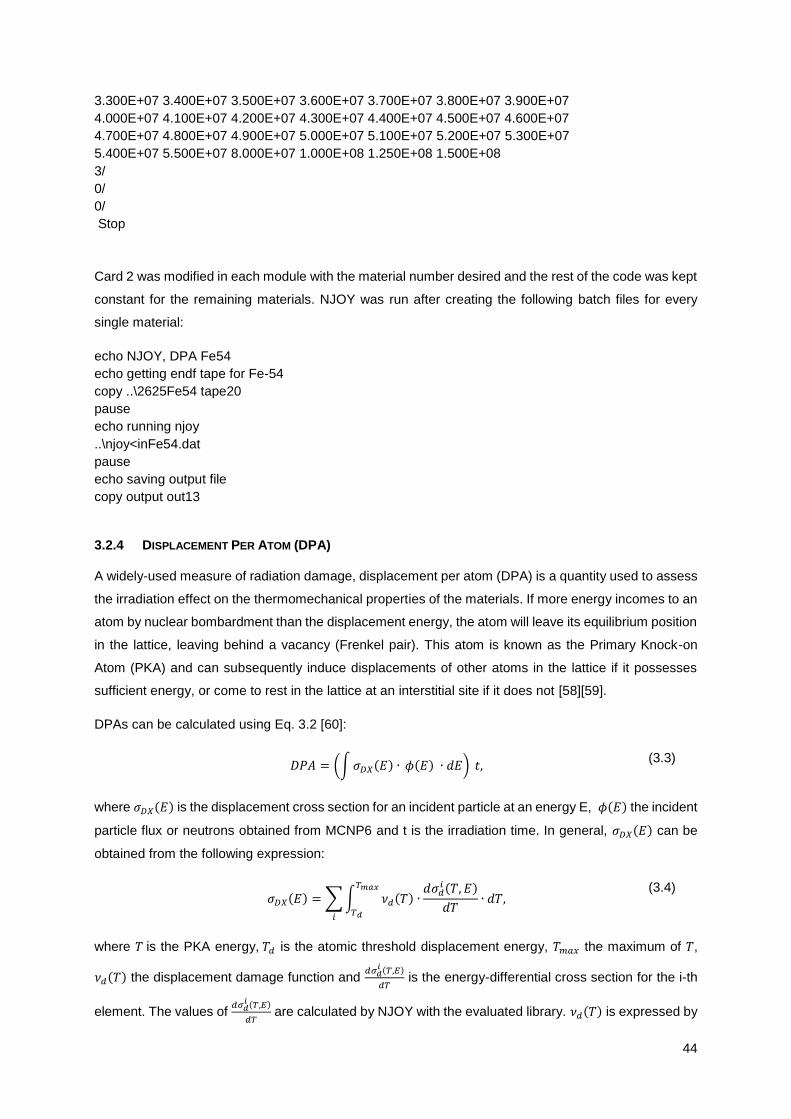
44
3.300E+07 3.400E+07 3.500E+07 3.600E+07 3.700E+07 3.800E+07 3.900E+07
4.000E+07 4.100E+07 4.200E+07 4.300E+07 4.400E+07 4.500E+07 4.600E+07
4.700E+07 4.800E+07 4.900E+07 5.000E+07 5.100E+07 5.200E+07 5.300E+07
5.400E+07 5.500E+07 8.000E+07 1.000E+08 1.250E+08 1.500E+08
3/
0/
0/
Stop
Card 2 was modified in each module with the material number desired and the rest of the code was kept
constant for the remaining materials. NJOY was run after creating the following batch files for every
single material:
echo NJOY, DPA Fe54
echo getting endf tape for Fe-54
copy ..\2625Fe54 tape20
pause
echo running njoy
..\njoy<inFe54.dat
pause
echo saving output file
copy output out13
3.2.4 DISPLACEMENT PER ATOM (DPA)
A widely-used measure of radiation damage, displacement per atom (DPA) is a quantity used to assess
the irradiation effect on the thermomechanical properties of the materials. If more energy incomes to an
atom by nuclear bombardment than the displacement energy, the atom will leave its equilibrium position
in the lattice, leaving behind a vacancy (Frenkel pair). This atom is known as the Primary Knock-on
Atom (PKA) and can subsequently induce displacements of other atoms in the lattice if it possesses
sufficient energy, or come to rest in the lattice at an interstitial site if it does not [58][59].
DPAs can be calculated using Eq. 3.2 [60]:
𝐷𝑃𝐴 = (∫𝜎𝐷𝑋(𝐸) ∙ 𝜙(𝐸) ∙ 𝑑𝐸) 𝑡,
(3.3)
where 𝜎𝐷𝑋(𝐸) is the displacement cross section for an incident particle at an energy E, 𝜙(𝐸) the incident
particle flux or neutrons obtained from MCNP6 and t is the irradiation time. In general, 𝜎𝐷𝑋(𝐸) can be
obtained from the following expression:
𝜎𝐷𝑋(𝐸) = ∑∫ 𝜈𝑑(𝑇) ∙
𝑑𝜎𝑑𝑖 (𝑇, 𝐸)
𝑑𝑇∙ 𝑑𝑇,
𝑇𝑚𝑎𝑥
𝑇𝑑𝑖
(3.4)
where 𝑇 is the PKA energy, 𝑇𝑑 is the atomic threshold displacement energy, 𝑇𝑚𝑎𝑥 the maximum of 𝑇,
𝜈𝑑(𝑇) the displacement damage function and 𝑑𝜎𝑑
𝑖 (𝑇,𝐸)
𝑑𝑇 is the energy-differential cross section for the i-th
element. The values of 𝑑𝜎𝑑
𝑖 (𝑇,𝐸)
𝑑𝑇 are calculated by NJOY with the evaluated library. 𝜈𝑑(𝑇) is expressed by

45
the following equation proposed by Norgett, Torrens and Robinson, based on the earlier Kinchin-Pease
model [61].
𝜈𝑑(𝑇) =
𝛽
2𝑇𝑑
∙ 𝑇𝑑𝑎𝑚 , (3.5)
where 𝛽 is the constant 0.8 [61], 𝑇𝑑𝑎𝑚 the damage energy and the 𝑇𝑑values are listed in Table 8 [62]:
Material Atomic displacement energy in
NJOY, Td (eV)
Be 31
C 31
Al 27
Cr 40
Fe 40
Ni 40
Cu 40
Pb 25
Table 8: Atomic displacement energy 𝑇𝑑 in NJOY (eV) for some materials.
The method used to obtain the DPAs is summarized in Figure 31.
DPAs can be calculated per lifetime and per year at full power capacity. Note that the F4 tally from
MCNP6 was left without normalisation as the source strength is not constant during the lifetime of ITER.
Table 9 shows the irradiation profile foreseen for ITER.
For each cell, a spreadsheet was created with the following columns:
Energy bins (MeV).
Tally F4 from MCNP6: Fluence per source particle.
Fluxes (neutrons and gamma/cm2s) obtained by multiplying fluence and source strengths. (Five
columns for every source strength).
NJOY cross sections in barns for every iron element (2625,2631,2634,2637).
Displacement Per Atom
(DPA)
Neutron fluxes
(MCNP6)
Energy-differential cross sections for each element (NJOY)
Figure 31: Flow chart showing the variables needed for calculating the DPAs.

46
Source strength
(source particle/s) Duration No. of times
1.0714×10¹⁷ 2 years 1
8.25×10¹⁷ 10 years 1
0 0.667 years 1
1.6607×10¹⁸ 1.33 years 1
0 3920 secs 17
2.0×10¹⁹ 400 secs
0 3920 secs
4 2.8×10¹⁹ 400 secs
Table 9: Source strength in ITER's lifetime.
Then for each i-isotope the DPAs per year were calculated for every source strength j:
𝐷𝑃𝐴𝑖,𝑗 (𝑦𝑒𝑎𝑟−1)
=𝜑(
𝑛 𝑜𝑟 𝑔𝑎𝑚𝑚𝑎𝑐𝑚2𝑠
) ∙ 𝜎(𝑏𝑎𝑟𝑛𝑠) ∙ 1x10⁻²⁴ (cm2
barn) ∙ 0.8 ∙ 3600 (
sh) ∗ 24 (
hday
) ∗ 365(dayyear
)
Td (eV)
(3.6)
DPAs in ITER’s lifetime for each isotope are calculated afterwards:
𝐷𝑃𝐴𝑖 (𝑙𝑖𝑓𝑒𝑡𝑖𝑚𝑒) = ∑𝐷𝑃𝐴𝑗
5
𝑗=1
(𝑝𝑒𝑟 𝑦𝑒𝑎𝑟) ∗ 𝑦𝑒𝑎𝑟𝑠, (3.7)
Finally, the overall effect on the different N isotopes is taken into account and integration is done over
the energy spectrum [63]:
𝐷𝑃𝐴 =
∫𝑑𝐸 𝜑(𝑟 , 𝐸)∑ 𝜌𝑖𝜎𝑅,𝐷𝑃𝐴,𝑖 (𝐸)𝑁𝑖=1
∑ 𝜌𝑖𝑁𝑖=1
, (3.8)
in which 𝜑(𝑟 , 𝐸) is the neutron flux (cm-2s-1MeV-1), 𝜌𝑖 is the atom density (barn-1cm-1) for isotope i and
𝜎𝑅,𝐷𝑃𝐴,𝑖 is the DPA cross section (barns/atom) for isotope i at energy E.

47
4 RESULTS
4.1 Shielding sphere
A geometry was implemented to see the effect of ionizing radiation and to serve as a model for the MMA
interface. Neutrons may interact with matter through elastic collisions, whereby energy is loss.
Depending on the atomic mass of the target nucleus, the average number of collisions required to
thermalize the neutrons is different. As Table 3 shows, the greater the atomic mass the higher the
average number of collisions needed.
Figure 32 shows the mesh tally obtained from MCNP6 for the lead-shielded sphere. The neutron flux in
lead is higher than the one estimated for the water-shielded sphere (See Figure 33). This shows that
water is indeed a better neutron moderator than lead, as discussed in section 2.2.1.
Figure 32: Neutron flux (n/cm2s) across the lead shielding cells.

48
Figure 33: Neutron flux (n/cm2s) across the water shielding cells.
Figure 34: Photon flux (Ɣ/cm2s) across the lead shielding cells.

49
According to the results in Figure 34 and Figure 35, there are lower photon fluxes in water than in lead.
Contrary to what happens with neutrons, this does not mean that water is a better shielding material for
photons than lead, which is not the case; it is rather due to the fact that in water the photons are produced
in the inner layers.
Figure 35: Photon flux (Ɣ/cm2s) across the water shielding cells.
More layers were added to improve the resolution of the results in the inner cells, following the
methodology described in section 3.1.1. The resulting geometry configuration is shown in Figure 36.

50
Figure 36: New geometry implemented.
Figure 37 shows the neutron flux spectra in each of the surfaces of the lead shielding. It can be seen
that as we get further away from the neutron source, the neutron and the photon fluxes are reduced at
all energies, as absorption of particles takes place.
Figure 37: Neutron flux across the lead shielding surfaces.
4,78E-01; 1,41E+13
1,00E+05
1,00E+06
1,00E+07
1,00E+08
1,00E+09
1,00E+10
1,00E+11
1,00E+12
1,00E+13
1,00E+14
1,00E-05 1,00E-04 1,00E-03 1,00E-02 1,00E-01 1,00E+00 1,00E+01
Neu
tro
n f
lux
in n
/cm
^2*s
Energy in MeV
Surface 2
Surface 3
Surface 4
Surface 5
Surface 6
Surface 7
Surface 8
Surface 9
Surface 10

51
Figure 38: Photon flux across the lead shielding surface.
When the 14-MeV neutrons released by the source interact with the shielding material, inelastic
scattering and radiative capture occur, resulting in the emission of photons with particular energies in
order to bring the nucleus back down to a stable or ground state. This explains the several peaks in the
photon flux spectra, at 11.6 keV, 82.5 keV, 53.1 keV and 7.5 MeV, as shown in Figure 38.
The neutron fluxes in water (see Figure 39) follow an irregular distribution but the spectra are softer than
in lead (Figure 37).
Figure 39: Neutron flux across the water shielding surfaces.
In water, Figure 40 shows that there are also peaks in the photon fluxes but they are concentrated in
the region from 2 to 10 MeV.
1,00E+06
1,00E+07
1,00E+08
1,00E+09
1,00E+10
1,00E+11
1,00E+12
1,00E-03 1,00E-02 1,00E-01 1,00E+00 1,00E+01
Ph
oto
n F
lux
(1
/cm
^2*s
)
Energy (MeV)
Surface 2
Surface 3
Surface 4
Surface 5
Surface 6
Surface 7
Surface 8
Surface 9
Surface 10
1,00E+06
1,00E+07
1,00E+08
1,00E+09
1,00E+10
1,00E+11
1,00E+12
1,00E+13
1,00E-05 1,00E-04 1,00E-03 1,00E-02 1,00E-01 1,00E+00 1,00E+01
Neu
tro
n f
lux
in n
/cm
^2*s
Energy in MeV
2
3
4
5
6
7
8
9
10

52
Figure 40: Photon fluxes across the water shielding surfaces.
The comparison between water and lead for surface 6 (75 cm of width) can be seen in Figure 41. The
higher neutron fluxes at higher energies in water are due to the fact that water has a much lower density
than lead, and therefore more un-collided neutrons reach surface 6 with water than with lead. For lower
energies, the fluxes are more similar. The exception is for energies between 0.025 eV and 10 eV, where
the fluxes are higher for water by more than one order of magnitude, which shows that water is more
effective at thermalizing neutrons.
Figure 41: Neutron and photon fluxes across the lead and water shielding surface 6.
1,00E+05
1,00E+06
1,00E+07
1,00E+08
1,00E+09
1,00E+10
1,00E+11
1,00E+12
1,00E+13
1,00E-03 1,00E-02 1,00E-01 1,00E+00 1,00E+01
Ph
oto
n f
lux
in g
amm
a/cm
^2*s
Energy in MeV
2
3
4
5
6
7
8
9
10
1,00E+06
1,00E+07
1,00E+08
1,00E+09
1,00E+10
1,00E+11
1,00E+12
1,00E+13
1,00E+14
1,00E+15
1,00E+16
1,00E-05 1,00E-04 1,00E-03 1,00E-02 1,00E-01 1,00E+00 1,00E+01 1,00E+02
Log
(Flu
x) in
par
ticl
e/cm
^2*s
Log (Energy) in MeV
Lead neutron flux Water neutron flux Lead photon flux Water photon flux

53
Figure 42 shows the heat loads in each cell for the two shielding materials. For water, more energy is
deposited in the first cell (cell number 2), whereas more energy is deposited in lead from cell 3 onwards.
Figure 42: Power density in each cell for the lead and water shielding layers.
Figure 43: Steady-state thermal analysis for lead shielding.
1,00E-08
1,00E-07
1,00E-06
1,00E-05
1,00E-04
1,00E-03
1,00E-02
1,00E-01
1,00E+00
0 2 4 6 8 10 12
Po
wer
den
sity
in W
/cm
^3
Cell number
Power density lead Power density water

54
The temperature distribution is shown in Figure 43 and Figure 44. Results show that both materials are
not suitable for the source intensity of 2x10¹⁹ source particles/s. The maximum temperature reached
with lead is 817.24 ºC, above the melting point of 327.5 ºC. Only the outer layers can withstand the
temperature. This happens because water has a very low conductivity when compared to lead, yielding
extremely high temperatures (of the order of 2.6x10⁵ ºC).
Figure 44: Steady-state thermal analysis for water shielding.
4.2 PPR system
4.2.1 POWER DENSITY
According to the methodology described in section 3.2.2 (MCNP procedure), the power density was
calculated for each cell, which is the total power density that the structure needs to withstand. The
estimated power density in the PPR in-vessel components due to ionizing radiation are presented in
Table 10. Relative contributions of neutrons and gamma photons to the energy deposition in each cell
are also achieved by simulation in MCNP6.
The most exposed parts to irradiation are the tips of the antennas, where the heat loads are predicted
to be of the order of 3.8 W/cm3, decreasing steadily up to cell 133414, which is already located behind

55
BM#11. There is an increase in energy deposition in cells 133415 and 133416 (located side-by-side)
due to an increase in heat load by photons while maintaining approximately the same heat load induced
by neutrons in cells 133414, 133415 and 133416. The power density for cells 133417,133418,133419
and 12231 are lower, implying thus that the opening between the blanket module and the upper port
has little effect on the power density in these cells.
Cell Total power density (W/cm3)
Stat. Error (%)
Power density by Neutrons (W/cm3)
Stat. Error (%)
Power density by
Neutrons (%)
Power density by
Photons (%)
133401 3.7361 1.92 0.5857 2.76 15.7 84.3
133402 3.7779 1.90 0.6028 2.78 16.0 84.0
133403 3.0941 2.21 0.4836 3.33 15.6 84.4
133404 3.0397 2.08 0.4687 3.12 15.4 84.6
133405 2.2791 2.45 0.4016 3.75 17.6 82.4
133406 2.9219 2.42 0.3668 3.68 12.6 87.4
133407 1.9908 3.43 0.3155 4.79 15.8 84.2
133408 1.9227 3.24 0.3091 5.00 16.1 83.9
133409 1.5103 1.67 0.2218 2.20 14.7 85.3
133410 0.8384 1.45 0.0995 1.89 11.9 88.1
133411 0.4726 1.84 0.0440 2.43 9.31 90.7
133412 0.2790 2.21 0.0237 2.89 8.49 91.5
133413 0.1698 2.20 0.0124 2.75 7.30 92.7
133414 0.1070 6.40 0.0049 7.27 4.58 95.5
133415 0.1342 4.77 0.0057 7.30 4.25 95.8
133416 0.1364 4.64 0.0048 6.08 3.52 96.5
133417 0.0831 4.14 0.0033 4.76 3.97 96.0
133418 0.0658 4.40 0.0031 6.45 4.71 95.2
133419 0.0753 8.70 0.0037 11.8 4.91 95.1
12230 0.0072 6.36 0.0004 9.08 5.56 94.4
12231 0.0868 3.60 0.0044 4.85 5.07 94.9
Table 10: Power density in the PPR components of gap 4.
It is clear that photons contribute the most, from approximately 84% to 96.5% of the total heat load. This
is due to the fact that PPR components are made of stainless steel, a High-Z material and therefore
more effective to shield photons than neutrons (see Section 4.1). The statistical errors of all tallies are
below 10% except for cell 133419. This is due to the large amount of CPU time that is required in order
to perform the simulations with such a complex geometry. The results of cell 133419 are, however,
consistent with the results obtained for the neighbouring cells.
4.2.2 TEMPERATURE DISTRIBUTION
The results in the PPR system for the temperature were obtained in a previous work [64], following the
methodology described in section 3.3.1, and are included here to complement the analysis. The 20-

56
node thermal FEs were chosen with a single degree-of-freedom at each node (temperature). The
following boundary conditions were used:
An environment temperature of 150ºC.
A radiation power per unit area of 500 kW/m2.
At first, it is considered that the system will reach the steady-state regime in order to prove the
consistency of the model.
Furthermore, it is assumed that the material is a grey body, the absorptivity is equal to the emissivity,
which, like other properties, is dependent on the temperature. Two emissivity conditions were applied:
a. the exterior and inner surfaces of the antenna have equal emissivity values.
b. the exterior surface of the antenna has an emissivity value similar to that of the blanket
modules surfaces, whereas the inner surfaces of the antenna keep the initial emissivity
values.
Figure 45: Steady-state temperature distribution of the PPR in-vessel components [64].
Figure 45 illustrates that the maximum temperature achieved is at the tips of the antennas:
approximately 759ºC for emissivity condition a) and 714ºC for emissivity condition b). [64]. Hence,
emissivity condition b) is recommended for lower temperature operation.

57
Figure 46: Transient temperature analysis for emissivity conditions #1 (a) and #2 (b) [64].
As for the transient temperature analysis, it is considered that ITER will operate in 400-second cycles
and with an initial temperature of 150ºC. Figure 46 shows that steady-state conditions are not achieved;
temperatures are lower than the ones obtained in Figure 45 .
For emissivity condition a), the tips of the antennas reach a maximum temperature of approximately
713ºC. For emissivity condition b), the tips of the antennas reach a maximum temperature of
approximately 702ºC [64]. Thus, emissivity condition b) is again recommended, although the tips of the
antennas present lower maximum temperatures before t=350 s.
4.2.3 DPAS
According to the methodology described in sections 3.2.2 and 3.2.4, the energy cross sections were
obtained from NJOY and the library FENDL 3.1. Figure 47 shows the output from NJOY compared to
the latest set of cross sections available in the JANIS program (FENDL2.1). The comparison illustrates
how NJOY changes from pointwise cross sections to energy groups.
The material chosen as an approximation for stainless steel 316L (N)-IG is natural iron, for which the
value of Td is 40 eV. For every single isotope, DPAs are calculated over all the spectrum, slightly
overestimating results as there is a low boundary of 40 eV that is not considered. Figure 48 shows the
cross sections obtained from NJOY in barns for the four isotopes of natural iron. DPAs are summed up
according to their weight composition: Fe-54 is 5.845%, Fe-56 is 91.754%, Fe-57 is 2.119% and 0.282%
of the composition of natural iron is Fe-58.

58
Figure 47: Damage energy cross section for iron isotope in barns.
Figure 48: Cross sections obtained from NJOY in barns for the four isotopes of natural iron.
The DPA results are summarized in Table 12. DPAs reach a maximum value of 1.2 during the lifetime
of ITER at the antenna tips for being exposed to higher levels of neutron fluxes for cells 133401 and
133402. Note that the DPA calculated is approximately the same for cell 133401, as they are adjacent
cells and exposed to the approximately the same neutron fluence. In general terms, DPAs are
decreasing at a steady rate as the neutron fluence decreases as shown in Figure 49 and
1,00E+00
1,00E+01
1,00E+02
1,00E+03
1,00E+04
1,00E+05
1,00E+06
1,00E-11 1,00E-09 1,00E-07 1,00E-05 1,00E-03 1,00E-01 1,00E+01
Cro
ss s
ecti
on
(b
arn
s)
Energy (MeV)
2625 2631 2634 2637

59
Table 11.
Figure 49: Neutron fluence for the two cells selected.
Cell number Neutron fluence
(n/cm2sourceparticle)
Neutron flux at full power (n/cm2s)
Total statistical error (%)
133401 4.89E-06 9.78E+13 1.13
133402 4.90E-06 9.80E+13 1.12
133403 4.32E-06 8.65E+13 1.26
133404 4.26E-06 8.53E+13 1.23
133405 3.69E-06 7.37E+13 1.39
133406 3.67E-06 7.34E+13 1.38
133407 3.20E-06 6.40E+13 1.75
133408 3.15E-06 6.30E+13 1.75
133409 2.70E-06 5.39E+13 0.91
133410 1.84E-06 3.68E+13 0.83
133411 1.20E-06 2.41E+13 0.95
133412 8.20E-07 1.64E+13 1.05
133413 5.60E-07 1.12E+13 1.08
133414 3.60E-07 7.20E+12 2.35
133415 3.14E-07 6.28E+12 2.13
133416 3.30E-07 6.59E+12 1.98
133417 2.55E-07 5.10E+12 1.81
133418 2.48E-07 4.96E+12 1.75
133419 2.59E-07 5.19E+12 3.01
12230 2.41E-08 4.83E+11 2.11
12231 3.27E-07 6.54E+12 1.30
Table 11: Neutron fluence, neutron flux at full power and total statistical error from MCNP6.

60
The DPAs calculated at full power capacity with an intensity of 2x10¹⁹ particles/s are less than double
the DPAs reached in ITER’s lifetime. This is due to the short period under which the PPR in-vessel
components are exposed to full power capacity: 17 cycles of 400 seconds exposure combined with 3920
seconds without irradiation.
In addition, DPAs are within the expected values for a fusion reactor: according to reference [65], the
maximum value expected for ITER in the blanket is 3 DPA.
Cell number DPA (in ITER’s lifetime) DPA (per year 500MW)
133401 1,19E+00 2,22E+00
133402 1,20E+00 2,25E+00
133403 9,89E-01 1,85E+00
133404 9,71E-01 1,82E+00
133405 8,34E-01 1,56E+00
133406 7,86E-01 1,47E+00
133407 6,70E-01 1,25E+00
133408 6,66E-01 1,25E+00
133409 5,01E-01 9,38E-01
133410 2,60E-01 4,86E-01
133411 1,33E-01 2,49E-01
133412 7,74E-02 1,45E-01
133413 4,63E-02 8,67E-02
133414 2,25E-02 4,21E-02
133415 2,10E-02 3,93E-02
133416 2,05E-02 3,84E-02
133417 1,53E-02 2,87E-02
133418 1,47E-02 2,75E-02
133419 1,73E-02 3,24E-02
12230 1,67E-03 3,13E-03
12231 2,16E-02 4,04E-02 Table 12: DPAs per lifetime and per year at full power capacity for every cell.
Results are also complemented with FISPACT [66] calculations performed in the group, which are
provided in Table 13 to show the production of H and He in one of the cells exposed to higher radiation
levels (133401). It can be seen that the production of He in stainless steel (32 appm) is below the
maximum value of 75 appm predicted in reference [65]. As there are many more elements in stainless
steel than in iron, the appm values for H and He are much higher in the former.
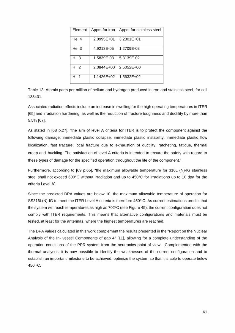
61
Table 13: Atomic parts per million of helium and hydrogen produced in iron and stainless steel, for cell
133401.
Associated radiation effects include an increase in swelling for the high operating temperatures in ITER
[65] and irradiation hardening, as well as the reduction of fracture toughness and ductility by more than
5,5% [67].
As stated in [68 p.27], “the aim of level A criteria for ITER is to protect the component against the
following damage: immediate plastic collapse, immediate plastic instability,immediate plastic flow
localization,fast fracture,local fracture due to exhaustion of ductility, ratcheting,fatigue,thermal
creep andbuckling. The satisfaction of level A criteria is intended to ensure the safety with regard to
these types of damage for the specified operation throughout the life of the component.”
Furthermore, according to [69 p.65], “the maximum allowable temperature for 316L (N)-IG stainless
steel shall not exceed 600°C without irradiation and up to 450°C for irradiations up to 10 dpa for the
criteria Level A”.
Since the predicted DPA values are below 10, the maximum allowable temperature of operation for
SS316L(N)-IG to meet the ITER Level A criteria is therefore 450º C. As current estimations predict that
the system will reach temperatures as high as 702ºC (see Figure 45), the current configuration does not
comply with ITER requirements. This means that alternative configurations and materials must be
tested, at least for the antennas, where the highest temperatures are reached.
The DPA values calculated in this work complement the results presented in the “Report on the Nuclear
Analysis of the In- vessel Components of gap 4“ [11], allowing for a complete understanding of the
operation conditions of the PPR system from the neutronics point of view. Complemented with the
thermal analyses, it is now possible to identify the weaknesses of the current configuration and to
establish an important milestone to be achieved: optimize the system so that it is able to operate below
450 ºC.
Element Appm for iron Appm for stainless steel
He 4 2.0995E+01 3.2301E+01
He 3 4.9213E-05 1.2709E-03
H 3 1.5839E-03 5.3139E-02
H 2 2.0844E+00 2.5052E+00
H 1 1.1426E+02 1.5632E+02

62
5 CONCLUSION AND FUTURE WORK
As a first step in this work, a shielding sphere was implemented in order learn the basics regarding the
interaction of neutrons and photons with matter and how the nuclear energy deposition in the materials
is translated from MCNP to ANSYS in order to obtain the operation temperatures. Results show that
High-Z materials are appropriate for stopping photons, whereas Low-Z materials are suitable for neutron
shielding, as expected. An example is lead, which is used as a shielding material for photons, and water,
which is mainly used in nuclear power plants to moderate neutrons. When analysing photons through
the mesh tally, there is a higher flux in lead due to the increase in production of photons in the outer
cells. Finally, the temperature distribution is analysed, showing that both materials (especially water) will
reach high temperatures when exposed to a source of neutrons with an intensity comparable to the one
foreseen for ITER.
In addition, the interface MMA allows for an automatic translation between MCNP and ANSYS with the
capability of changing the following parameters: conductivity and density of the material, atomic number
of the element used as shielding material, source intensity and ambient temperature. The automatized
procedure allows the user to save time when calculating the temperature distribution on the sphere
under different operation conditions.
According to the results obtained in the PPR, the power density is greater at the tips of the antennas,
as they are exposed to higher levels of neutron and photon fluxes. Furthermore, emissivity condition b),
where the outer surfaces of the PPR components have the same value of the emissivity of the blanket
module, is recommended as a solution to decrease the temperature. However, 702ºC still exceeds the
maximum allowable temperature of 450ºC for irradiations up to 10 DPA, necessary to comply with the
ITER requirements. Nevertheless, the DPA values are within the expected margins (1.2 DPA per
lifetime) and may be used to analyse effects such as swelling and reduction in ductility.
An optimization study showed that by increasing the thickness of the antennas, a temperature decrease
of approximately 100ºC can be achieved. Another possible solution is the shift of the position of the PPR
backwards in order to decrease neutron and photon irradiation, which, however, may compromise the
performance of the system. The change of material is another possibility, tungsten being a potential
candidate, due to its high melting point and resistance to irradiation.
Hopefully, I will continue this work during my Ph.D. and be able to perform a complete neutronics and
mechanical analysis, as well as extend the development of the MMA interface for different
configurations.

63
BIBLIOGRAPHY
[1] EIA, “International Energy Outlook 2013 with Projections to 2040,” 2016.
[2] International Energy Agency, “Redrawing the energy-climate map,” 2013.
[3] NOAA Earth System Research Laboratory, “Trends in Atmospheric Carbon Dioxide.” [Online].
Available: http://www.esrl.noaa.gov/gmd/ccgg/trends/global.html. [Accessed: 24-Jul-2016].
[4] J. P. Friedberg, Plasma Physics and Fusion Energy. Cambridge University Press, 2007.
[5] J. M. Perlado Martín, “La fusión nuclear como fuente masiva de energía,” 2010.
[6] ITER, “When will experiments begin?,” 2016. [Online]. Available:
https://www.iter.org/proj/inafewlines#6. [Accessed: 22-Aug-2016].
[7] P. Rincon, “UK centre to shoot for nuclear fusion record.” [Online]. Available:
http://www.bbc.com/news/science-environment-27138087.
[8] “ITER 2010.” [Online]. Available: http://www.fusion.kit.edu/img/ITER_2010.jpg. [Accessed: 07-
Sep-2016].
[9] ITER EDA, “Summary of the ITER Final Design Report,” 2001.
[10] P. Varela, “PPR System Design Description Document.”
[11] R. Fernandes Luis, “Nuclear analysis of the PPR in-vessel components of gap 4.,” 2016.
[12] IPFN, “ITER Plasma Position Reflectometry (PPR) Diagnostic System.,” 2013. [Online].
Available: http://www.ipfn.tecnico.ulisboa.pt/F4E_FPA375/index.html. [Accessed: 28-Aug-2016].
[13] R. Nave, “Nuclear Fusion.” [Online]. Available: http://hyperphysics.phy-
astr.gsu.edu/hbase/nucene/fusion.html. [Accessed: 27-Aug-2016].
[14] Eurofusion, “https://www.euro-fusion.org/faq/how-are-alpha-particles-produced-and-how-
dangerous-are-they/.” [Online]. Available: https://www.euro-fusion.org/faq/how-are-alpha-
particles-produced-and-how-dangerous-are-they/. [Accessed: 27-Aug-2016].
[15] Fusion For Energy, “What is fusion?” [Online]. Available:
http://fusionforenergy.europa.eu/understandingfusion/. [Accessed: 02-Aug-2016].
[16] P. Batistoni, “Neutrons: little particles with powerful impact,” March,18., 2016. [Online]. Available:
https://www.euro-fusion.org/newsletter/neutrons-little-particles-with-powerful-impact/.
[Accessed: 02-Aug-2016].
[17] ITER, “Tritium Breeding.” [Online]. Available: https://www.iter.org/mach/TritiumBreeding.
[Accessed: 07-Sep-2016].
[18] J. P. Friedberg, Plasma Physics and Fusion Energy. Cambridge University Press, 2007.
[19] F. Wagner, G. Becker, K. Behringer, D. Campbell, A. Eberhagen, W. Engelhardt, G. Fussmann,
O. Gehre, J. Gernhardt, G. V. Gierke, G. Haas, M. Huang, F. Karger, M. Keilhacker, O. Kl̈ber, M.

64
Kornherr, K. Lackner, G. Lisitano, G. G. Lister, H. M. Mayer, D. Meisel, E. R. M̈ller, H. Murmann,
H. Niedermeyer, W. Poschenrieder, H. Rapp, H. Röhr, F. Schneider, G. Siller, E. Speth, A.
Stäbler, K. H. Steuer, G. Venus, O. Vollmer, and Z. Ÿ, “Regime of improved confinement and
high beta in neutral-beam-heated divertor discharges of the ASDEX tokamak,” Phys. Rev. Lett.,
vol. 49, no. 19, pp. 1408–1412, 1982.
[20] H. Zohm, “Edge localized modes (ELMs),” Plasma Phys. Control. Fusion, vol. 38, no. 2, pp. 105–
128, 1996.
[21] I. Olegovich, “Impurity Transport Studies on Alcator C-Mod Tokamak Using Charge Exchange
Recombination Spectroscopy,” University of Texas, 2008.
[22] J. Mlynár and M. Ripa, “50 years of tokamaks,” 2008. [Online]. Available: https://www.euro-
fusion.org/newsletter/50-years-of-tokamaks/. [Accessed: 08-Sep-2016].
[23] T. and I. of B. Ministery of Science, “Plasma Confinement.” [Online]. Available:
http://www.plasma.inpe.br/LAP_Portal/LAP_Site/Text/Plasma_Confinement.htm. [Accessed:
08-Oct-2016].
[24] J. D. Lawson, “Some Criteria for a Power Producing Thermonuclear Reactor,” Proc. Phys. Soc.
Sect. B, vol. 70, no. 1, pp. 6–10, 1957.
[25] R. Tilley, Understanding solids: the science of materials. John Wiley & Sons, 2005.
[26] T. Jevremovic, Nuclear principles in engineering (Second edition). 2009.
[27] A. Poch, Radiaciones ionizantes. Utilización y riesgos. Edicions UPC, 1994.
[28] K. S. Krane, Introductory Nuclear Physics. John Wiley and Sons, 1988.
[29] IAEA, “Measurement of residual stress in materials using neutrons,” 2013.
[30] E. Gallego Díaz, “Dosimetría de neutrones. Dispositivos para detección y dosimetría de
neutrones.” 2008.
[31] D.J.H. and R.B.S., “Neutron cross sections,” J. Nucl. Energy, vol. 7, no. 3–4, p. 228, 1958.
[32] J. J. Duderstadt and L. J. Hamilton, “Nuclear Reactor Analysis,” Mechanical Engineering, vol.
31, no. 4. pp. 138–142, 1976.
[33] C. D. B. Roald Amundsen Schrack, “Nuclear Cross Sections and Technology,” 1975.
[34] R. Fernandes Luis, “Radiological Protection and Nuclear Engineering Studies in Multi-MW Target
Systems,” 2013.
[35] K.-H. Beckurts and K. Wirtz, Neutron Physics. Springer Science & Business Media, 2013.
[36] P. Rinard, “Neutron interactions with matter,” in Passive Nondestructive Assay of Nuclear
Materials, D. Reily, N. Ensslin, and H. ; Smith, Eds. 1991.
[37] U. Doe, “Doe-hdbk-1019/1-93 nuclear physics and reactor theory,” Nucl. Phys., vol. 1, no.
January, pp. 2238–2239, 1993.

65
[38] X. Qiu, “Neutron Interaction with Germanium Detector.” [Online]. Available:
http://www.hep.umn.edu/cdms/geant4benchmark/050712/NwithGe.html. [Accessed: 08-Oct-
2016].
[39] R. F. Cleveland and J. L. Ulcek, “Questions and Answers about Biological Effects and Potential
Hazards of Radiofrequency Electromagnetic Fields.,” OET Bull. 56, vol. 4th editio, 1999.
[40] European Centre of Technological Safety, “Interaction of Radiation with Matter. Radiation
Hazard.” [Online]. Available: http://www.tesec-int.org/TechHaz-site 08/Radiation-interaction.pdf.
[Accessed: 05-Sep-2016].
[41] J. H. Hubbell, “Review of photon interaction cross section data in the medical and biological
context.,” Phys. Med. Biol., vol. 44, no. 1, pp. R1–R22, 1999.
[42] J. A. Seibert and J. M. Boone, “X-Ray Imaging Physics for Nuclear Medicine Technologists. Part
2: X-Ray Interactions and Image Formation,” J. Nucl. Med. Technol., vol. 33, 2005.
[43] X-5 Monte Carlo Team, “MCNP - A General Monte Carlo N-Particle Transport Code, Version 5,”
Los Alamos Nucl. Lab., vol. I, pp. 2-71-2–80, 2005.
[44] I. Sobol, A Primer for the Monte Carlo Method. CRC Press, 1994.
[45] A. F. Bielajew, “Fundamentals of the Monte Carlo method for neutral and charged particle
transport,” Sci. York, pp. 1–338, 2001.
[46] E. Gargioni, “Recent Progress in Radiation Transport Simulation Calculations: Available Codes.,”
2012.
[47] A. Davis, “Radiation shielding of fusion systems,” 2010.
[48] B. J.F, “MCNPTM – A General Monte Carlo N-Particle Transport Code, Version 4C,” Los Alamos
Natl. Lab., no. March, 2000.
[49] H. Policarpo, “Numerical and experimental models for vibration attenuation using cork composite
materials,” IST, 2013.
[50] S. Moaveni, Finite Element Analysis. Theory and Application with Ansys. Prentice-Hall, 1999.
[51] F. P. Incropera, D. P. DeWitt, T. L. Bergman, and A. S. Lavine, Fundamentals of Heat and Mass
Transfer, vol. 6th. 2007.
[52] Y. Zhan and M. Ning, “Galerkin Method.” [Online]. Available: http://www.sd.ruhr-uni-
bochum.de/downloads/Galerkin_method.pdf. [Accessed: 01-Jan-2016].
[53] J. Stewart, “Calculus, concepts and contexts,” Cole, Pacific Grove, CA, p. 1131, 1998.
[54] J. K. Shultis and R. E. Faw, “An MCNP Primer,” Structure, vol. 66506, no. c, pp. 0–45, 2006.
[55] J. T. Goorley, M. R. James, T. E. Booth, F. B. Brown, J. S. Bull, L. J. Cox, J. W. Durkee, J. S.
Elson, M. L. Fensin, R. A. Forster, J. S. Hendricks, H. G. Hughes, R. C. Johns, B. C. Kiedrowski,
R. L. Martz, S. G. Mashnik, G. W. McKinney, D. B. Pelowitz, R. E. Prael, J. E. Sweezy, L. S.
Waters, T. A. Wilcox, and A. Zukaitis, “MCNP6TM User’s Manual.” 2013.

66
[56] Y. W. Y. Li, L. Lu, A. Ding, H. Hu, Q. Zeng, S. Zheng, “Benchmarking of MCAM 4.0 with the ITER
3D model,” Proc. 24th Symp. Fusion Technol. — SOFT-24, vol. 82, no. 15–24, pp. 2861–2866,
2007.
[57] R. E. Macfarlane, D. W. Muir, R. M. Boicourt, and A. C. Kahler, “The NJOY Nuclear Data
Processing System, Version 2012,” LA-UR-12-27079, Los Alamos Natl. Lab., 2012.
[58] J. Chang and W. J. Lee, “Generation of damage cross section for silicon carbide,” 2013.
[59] G. H. Kinchin and R. S. Pease, “The Displacement of Atoms in Solids by Radiation.,” 1955.
[60] M. Harada, N. Watanabe, C. Konno, S. Meigo, Y. Ikeda, and K. Niita, “DPA calculation for
Japanese spallation neutron source,” in Journal of Nuclear Materials, 2005, vol. 343, no. 1–3,
pp. 197–204.
[61] M. J. Norgett, M. T. Robinson, and I. M. Torrens, “A proposed method of calculating displacement
dose rates,” Nucl. Eng. Des., vol. 33, pp. 50–54, 1975.
[62] American Society for Testing and Materials Annual, “Annual Book of ASTM Standards.,” vol.
Sec., 4. 1992.
[63] A. Hogenbirk, “An easy way to perform a radiation damage calculation in a complicated
geometry,” Fusion Eng. Des., vol. 83, no. 10–12, pp. 1828–1831, 2008.
[64] P. Quental, H. Policarpo, and R. Luis, “Thermal analysis of the in-vessel components of the ITER
Plasma Position Reflectometry,” 2016.
[65] L. K. Mansur, A. F. Rowcliffe, R. K. Nanstad, S. J. Zinkle, W. R. Corwin, and R. E. Stoller,
“Materials needs for fusion, Generation IV fission reactors and spallation neutron sources -
Similarities and differences,” in Journal of Nuclear Materials, 2004, vol. 329–333, no. 1–3 PART
A, pp. 166–172.
[66] J.-C. C. Sublet, J. W. Eastwood, J. G. Morgan, M. Fleming, and M. R. Gilbert, “The FISPACT-II
User Manual,” 2015.
[67] E. V. van Osch, M. G. Horsten, and M. I. de Vries, “Irradiation testing of 316L(N)-IG austenitic
stainless steel for ITER,” J. Nucl. Mater., 1998.
[68] V. Barabash, “In-vessel Components, SDC-IC,” 2012.
[69] V. Barabash, “Appendix A, Materials Design Limit Data,” 2013.

67
ANNEX I: MCNP6 CODE FOR SHIELDING SPHERE
(SHIELDINGSPHERE.TXT)
C Cell cards
1 0 -1 $source
2 1 -1 1 -2 $8 water shielding layers
3 1 -1 2 -3
4 1 -1 3 -4
5 1 -1 4 -5
6 1 -1 5 -6
7 1 -1 6 -7
8 1 -1 7 -8
9 1 -1 8 -9
10 1 -1 9 -10
11 2 -1 -11 $water sphere
12 0 11 10 -12 $cell around the water sphere
13 0 12 $outer space
C Surface cards
1 So 400 $sphere source radius R=4 m
2 So 420 $shielding layers
3 So 440
4 So 460
5 So 480
6 So 500
7 So 600
8 So 700
9 So 800
10 So 900
11 SZ 910 10
12 So 1000
C Data cards
mode n p
IMP:N,P 1 1 1 1 1 1 1 1 1 1 1 1 0
SDEF pos=0 0 0 rad=d1 cel=1 erg=14 par=N
SI1 0 400 $ radial sampling range: 0 to Rmax
SP1 -21 2 $ weighting for radial sampling: here r^2
F2:N 2 3 4 5 6 7 8 9 10 $average neutron fluxes across each shielding surface
E2 1e-5 100log 20 $from 10 eV to 20 MeV takes log spacing
F12:P 2 3 4 5 6 7 8 9 10
E12 1e-3 100log 20
F4:N 11 $neutron flux across the water sphere cell
E4 1e-5 100log 20
F14:P 11
E14 1e-3 100log 20 $Energy photons!
F6:N,P 2 3 4 5 6 7 8 9 10 $energy deposition across each shielding cell
NPS 100000

68
c tmesh
c rmesh31:n FLUX
c cora31 -1000 99i 1000
c corb31 -400 4i 400
c corc31 -1000 99i 1000
c endmd
c fm31 1.97e19
M2 1001 2 8016 1 $Water
fm4 1.97e19

69
ANNEX II: ANSYS APDL (SHIELDINGSPHERE.INP)
RUN_BATCH=1 !* 0 for manually and 1 for batch
!*====================================================================
/PREP7
*IF,RUN_BATCH,EQ,0,then
FINISH
/CLEAR,START
/COM,ANSYS RELEASE Release 17.1 BUILD 17.1 UP20160404 02:39:39
/input,start,ans,'C:\Program Files\ANSYS Inc\v171\ANSYS\apdl\'
!*
/PREP7
KXXa=35.3 !Conductivity
DENSa=11340 !Density
HGEN1=422035 !Heat generation
HGEN2=117225
HGEN3=7.467430000000000e+04
HGEN4=1.844320000000000e+04
HGEN5=1.084160000000000e+04
HGEN6=9.230940000000000e+03
HGEN7=0.002902050000000
HGEN8=0
HGEN9=0
Tempout=298.15 !Temperature outer layer (K)
!HGEN1=5000 !Heat generation
!HGEN2=5000
!HGEN3=5000
!HGEN4=5000
!HGEN5=5000
!HGEN6=5000
!HGEN7=5000
!HGEN8=5000
!HGEN9=5000
*ELSE
!******READ INPUT DATA FROM FILES***********
*DIM,out,ARRAY,1
*VREAD,out(1),Temp_MatL,TXT
(F13.2)
Tempout=out(1)
*DIM,condu,ARRAY,1
*VREAD,condu(1),KXX_MatL,TXT
(F13.2)
KXXa=condu(1)

70
*DIM,RHOa,ARRAY,1
*VREAD,RHOa(1),RHO_MatL,TXT
(F13.0)
DENSa=RHOa(1)
*DIM,HGEN1a,ARRAY,1
*VREAD,HGEN1a(1),HGEN1_MatL,TXT
(F13.0)
HGEN1=HGEN1a(1)
*DIM,HGEN2a,ARRAY,1
*VREAD,HGEN2a(1),HGEN2_MatL,TXT
(F13.0)
HGEN2=HGEN2a(1)
*DIM,HGEN3a,ARRAY,1
*VREAD,HGEN3a(1),HGEN3_MatL,TXT
(F13.0)
HGEN3=HGEN3a(1)
*DIM,HGEN4a,ARRAY,1
*VREAD,HGEN4a(1),HGEN4_MatL,TXT
(F13.0)
HGEN4=HGEN4a(1)
*DIM,HGEN5a,ARRAY,1
*VREAD,HGEN5a(1),HGEN5_MatL,TXT
(F13.0)
HGEN5=HGEN5a(1)
*DIM,HGEN6a,ARRAY,1
*VREAD,HGEN6a(1),HGEN6_MatL,TXT
(F13.0)
HGEN6=HGEN6a(1)
*DIM,HGEN7a,ARRAY,1
*VREAD,HGEN7a(1),HGEN7_MatL,TXT
(F13.0)
HGEN7=HGEN7a(1)
*DIM,HGEN8a,ARRAY,1
*VREAD,HGEN8a(1),HGEN8_MatL,TXT
(F13.0)
HGEN8=HGEN8a(1)
*DIM,HGEN9a,ARRAY,1
*VREAD,HGEN9a(1),HGEN9_MatL,TXT
(F13.0)
HGEN9=HGEN9a(1)
*ENDIF
ET,1,SOLID87

71
!*
MPTEMP,,,,,,,,
MPTEMP,1,0
MPDATA,KXX,1,,KXXa
MPDATA,DENS,1,,DENSa
!MPDATA,QRATE,1,,5
MPDATA,KXX,2,,KXXa
MPDATA,DENS,2,,DENSa
!MPDATA,QRATE,2,,50
MPDATA,KXX,3,,KXXa
MPDATA,DENS,3,,DENSa
!MPDATA,QRATE,3,,500
MPDATA,KXX,4,,KXXa
MPDATA,DENS,4,,DENSa
!MPDATA,QRATE,4,,5000
MPDATA,KXX,5,,KXXa
MPDATA,DENS,5,,DENSa
!MPDATA,QRATE,5,,50000
MPDATA,KXX,6,,KXXa
MPDATA,DENS,6,,DENSa
!MPDATA,QRATE,6,,5
MPDATA,KXX,7,,KXXa
MPDATA,DENS,7,,DENSa
!MPDATA,QRATE,7,,50
MPDATA,KXX,8,,KXXa
MPDATA,DENS,8,,DENSa
!MPDATA,QRATE,8,,500
MPDATA,KXX,9,,KXXa
MPDATA,DENS,9,,DENSa
!MPDATA,QRATE,9,,50000
SPH4, , ,4,4.2
SPH4, , ,4.2,4.4
SPH4, , ,4.4,4.6
SPH4, , ,4.6,4.8
SPH4, , ,4.8,5
SPH4, , ,5,6
SPH4, , ,6,7
SPH4, , ,7,8
SPH4, , ,8,9
/CPLANE,1
/ANG,1,30,XS,1
/REP,FAST
/TYPE,1,5
VSEL, , , , 1
VATT, 1, , 1, 0
VSEL, , , , 2
VATT, 2, , 1, 0
VSEL, , , , 3
VATT, 3, , 1, 0
VSEL, , , , 4

72
VATT, 4, , 1, 0
VSEL, , , , 5
VATT, 5, , 1, 0
VSEL, , , , 6
VATT, 6, , 1, 0
VSEL, , , , 7
VATT, 7, , 1, 0
VSEL, , , , 8
VATT, 8, , 1, 0
VSEL, , , , 9
VATT, 9, , 1, 0
!*
!*
MSHKEY,0
MSHAPE,1,3d
SMRTSIZE,8
VSEL, , , ,ALL
!*
VMESH,ALL
!*
DA,33,TEMP,Tempout
DA,34,TEMP,Tempout
BFV,1,HGEN,HGEN1
BFV,2,HGEN,HGEN2
BFV,3,HGEN,HGEN3
BFV,4,HGEN,HGEN4
BFV,5,HGEN,HGEN5
BFV,6,HGEN,HGEN6
BFV,7,HGEN,HGEN7
BFV,8,HGEN,HGEN8
BFV,9,HGEN,HGEN9
NUMMRG,ALL, , , ,LOW
NUMCMP,NODE
FINISH
/SOL
/STATUS,SOLU
SOLVE
FINISH
/POST1
!*
/EFACET,1
PLNSOL, TEMP,, 0
*get,NNODES,node,,num,max
!NNODES=5
*DIM,TT,ARRAY,(NNODES),1
*DO,I,1,(NNODES),1
*GET,TEMP%I%,NODE,%I%,TEMP
TT(I,1)=TEMP%I%

73
*ENDDO
/INPUT,ansuitmp
!*
*CREATE,ansuitmp
*CFOPEN,'TEMPERATURA','TXT',' '
*VWRITE,TT(1,1), , , , , , , , ,
(F22.15)
*CFCLOS
*END
/RGB,INDEX,100,100,100, 0
/RGB,INDEX, 80, 80, 80,13
/RGB,INDEX, 60, 60, 60,14
/RGB,INDEX, 0, 0, 0,15
/REPLOT
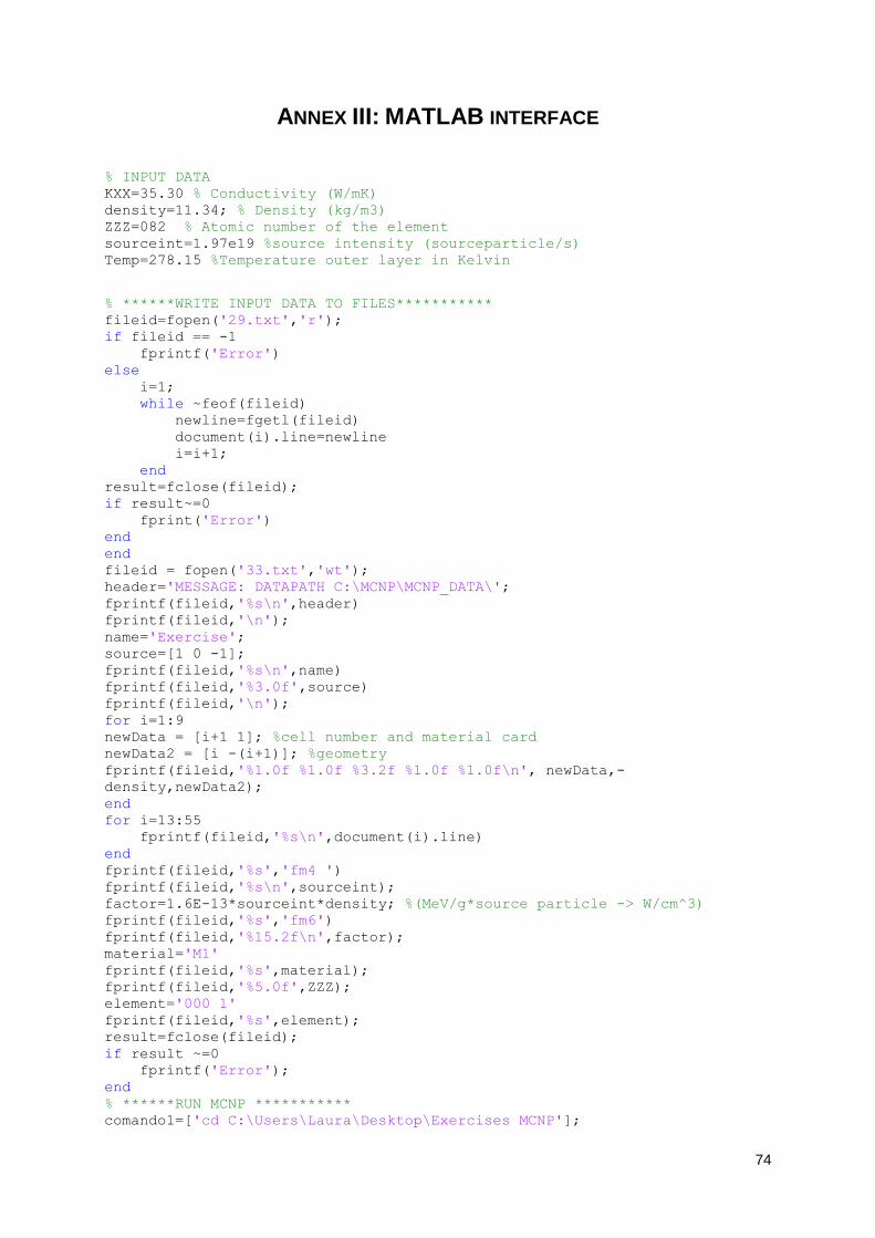
74
ANNEX III: MATLAB INTERFACE
% INPUT DATA KXX=35.30 % Conductivity (W/mK) density=11.34; % Density (kg/m3) ZZZ=082 % Atomic number of the element sourceint=1.97e19 %source intensity (sourceparticle/s) Temp=278.15 %Temperature outer layer in Kelvin
% ******WRITE INPUT DATA TO FILES*********** fileid=fopen('29.txt','r'); if fileid == -1 fprintf('Error') else i=1; while ~feof(fileid) newline=fgetl(fileid) document(i).line=newline i=i+1; end result=fclose(fileid); if result~=0 fprint('Error') end end fileid = fopen('33.txt','wt'); header='MESSAGE: DATAPATH C:\MCNP\MCNP_DATA\'; fprintf(fileid,'%s\n',header) fprintf(fileid,'\n'); name='Exercise'; source=[1 0 -1]; fprintf(fileid,'%s\n',name) fprintf(fileid,'%3.0f',source) fprintf(fileid,'\n'); for i=1:9 newData = [i+1 1]; %cell number and material card newData2 = [i -(i+1)]; %geometry fprintf(fileid,'%1.0f %1.0f %3.2f %1.0f %1.0f\n', newData,-
density,newData2); end for i=13:55 fprintf(fileid,'%s\n',document(i).line) end fprintf(fileid,'%s','fm4 ') fprintf(fileid,'%s\n',sourceint); factor=1.6E-13*sourceint*density; %(MeV/g*source particle -> W/cm^3) fprintf(fileid,'%s','fm6') fprintf(fileid,'%15.2f\n',factor); material='M1' fprintf(fileid,'%s',material); fprintf(fileid,'%5.0f',ZZZ); element='000 1' fprintf(fileid,'%s',element); result=fclose(fileid); if result ~=0 fprintf('Error'); end % ******RUN MCNP *********** comando1=['cd C:\Users\Laura\Desktop\Exercises MCNP'];

75
dos(comando1); s1='C:\MCNP\MCNP_CODE\bin\mcnp6.exe '; input='i=33.txt '; s2='n=run33_'; comando2=[s1 input s2]; dos(comando2); % ******RUN ANSYS *********** %% % ***************************************************** % CHECK IF RUN_BATCH IS SET TO 1 IN FILE BEAM.INP % *****************************************************
% INPUT DATA FOR ANSYS fileid=fopen('run33_o','r'); if fileid == -1 fprintf('Error') else i=1; while ~feof(fileid) newline=fgetl(fileid) document2(i).line=newline i=i+1; end result=fclose(fileid); if result~=0 fprint('Error') end end for i=1:28 line2=document2(4283); cell2=str2num(line2.line(1:28))*1000000; %convert to number and W/m^3 line3=document2(4286); cell3=str2num(line3.line(1:28))*1000000; line4=document2(4289); cell4=str2num(line4.line(1:28))*1000000; line5=document2(4292); cell5=str2num(line5.line(1:28))*1000000; line6=document2(4295); cell6=str2num(line6.line(1:28))*1000000; line7=document2(4298) cell7=str2num(line7.line(1:28))*1000000; line8=document2(4301); cell8=str2num(line8.line(1:28))*1000000; line9=document2(4304); cell9=str2num(line9.line(1:28))*1000000; line10=document2(4307); cell10=str2num(line10.line(1:28))*1000000; end % ******WRITE INPUT DATA TO FILES*********** rho=density*1000; fid = fopen('KXX_MatL.txt','w'); fprintf(fid,'%13.2f\n',KXX); fclose(fid); fid = fopen('RHO_MatL.txt','w'); fprintf(fid,'%13.0f\n',rho); fclose(fid); fid = fopen('HGEN1_MatL.txt','w'); fprintf(fid,'%13.0f\n',cell2); fclose(fid); fid = fopen('HGEN2_MatL.txt','w'); fprintf(fid,'%13.0f\n',cell3);

76
fclose(fid); fid = fopen('HGEN3_MatL.txt','w'); fprintf(fid,'%13.0f\n',cell4); fclose(fid); fid = fopen('HGEN4_MatL.txt','w'); fprintf(fid,'%13.0f\n',cell5); fclose(fid); fid = fopen('HGEN5_MatL.txt','w'); fprintf(fid,'%13.0f\n',cell6); fclose(fid); fid = fopen('HGEN6_MatL.txt','w'); fprintf(fid,'%13.0f\n',cell7); fclose(fid); fid = fopen('HGEN7_MatL.txt','w'); fprintf(fid,'%13.0f\n',cell8); fclose(fid); fid = fopen('HGEN8_MatL.txt','w'); fprintf(fid,'%13.0f\n',cell9); fclose(fid); fid = fopen('HGEN9_MatL.txt','w'); fprintf(fid,'%13.0f\n',cell10); fclose(fid); fid = fopen('Temp_MatL.txt','w'); fprintf(fid,'%13.2f\n',Temp); fclose(fid);
% ******RUN ANSYS IN BATCH MODE*********** entrada='shieldingsphere.inp'; s1='"C:\Program files\ANSYS Inc\v171\ansys\bin\winx64\ansys171.exe" -b -i
'; s2=' -o out.out'; comando=[s1 entrada s2]; dos(comando);
% *******RESULTS******* fidi = fopen('Temperatura.txt','r'); D = textscan(fidi, '%f%f%f%f%f', 'HeaderLines',1, 'CollectOutput',1); FileMax = max(D{:}(:)) fclose(fidi); fid = fopen('Maxtemp.txt','w'); fprintf(fid,'%13.0f\n',FileMax); fclose(fid);