evaluation of empirical models for calibration and ... · evaluation of empirical models for...
TRANSCRIPT

Evaluation of empirical modelsfor calibration and classification
2nd Summer School 2012 of the Marie Curie ITN "Environmental ChemoInformatics" and Meeting of the International Academy of Mathematical Chemistry,
11 - 15 June 2012, Verona, ItalyLecture 14 June 2012
Kurt VARMUZAVienna University of Technology
Institute of Chemical Engineeringand
Department of Statistics and Probability Theory
www.lcm.tuwien.ac.at, [email protected]
Collaboration: Peter Filzmoser and Bettina Liebmann
startVersion 120621, (C) K. Varmuza, Vienna, Austria

venus transit title
Contents1 Introduction2 Making empirical models
Calibration (OLS, PLS)Classification (DPLS, KNN)
3 Performance measuresCalibration (SEP, R2)Classification (predictive abilities)
4 StrategiesOptimum model complexityPerformance for new cases
5 Repeated double cross validationScheme - ResultsExample - Summary - Software
6 Conclusions
Acknowledgment. This work was supported by the Austrian Science Fund (FWF), project P22029-N13, "Information measures to characterize networks", project leader M. Dehmer (UMIT, Hall in Tyrol, Austria).

models general
desired datay (e.g., property)
Cannot be determined directly or only with high cost
Common situation in science
available datax1, x2, ..., xm= vector xT
Measured or calculated xj
modelŷ = f (x1, x2, ..., xm) = f (xT)
f: mathematical equation or algorithm,derived from data (empirical model) orfrom knowledge (theoretical model)

model fall.
stone
Common situation in science 1/3
x (height)
y (falling time)
Fundamental (scientific) law,first principle
ŷ = (2x / g) 0.5
model parameter g: gravity constant
available datax1, x2, ..., xm= vector xT
Measured or calculated xj
desired datay (e.g., property)
Cannot be determined directly or only with high cost
model NIR
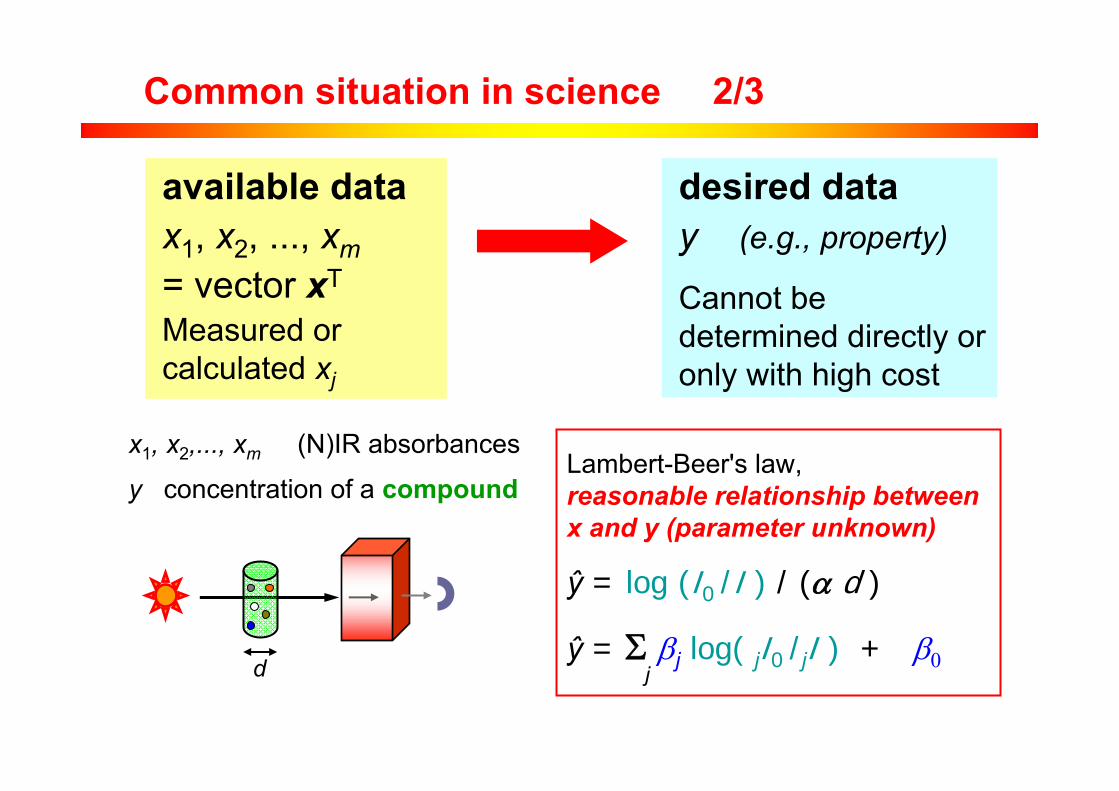
Common situation in science 2/3
x1, x2,..., xm (N)IR absorbances
y concentration of a compoundLambert-Beer's law,reasonable relationship between x and y (parameter unknown)
ŷ = log (I0 /I ) / ( d )
ŷ = j log( jI0 /jI ) + d j
available datax1, x2, ..., xm= vector xT
Measured or calculated xj
desired datay (e.g., property)
Cannot be determined directly or only with high cost

models QSPR
Common situation in science 3/3
Only an assumption:y (property) is simply related with x (variables),"very empirical" ("dangerous")
ŷ = x T b + b 0 (linear model)
property y
set of numbers,molecular descriptors, x T
available datax1, x2, ..., xm= vector xT
Measured or calculated xj
desired datay (e.g., property)
Cannot be determined directly or only with high cost

linmodel 1
ŷ = f (x1, x2, ..., xm)
y continuous multivariate calibration discrete, categorical multivariate classification
pattern recognition
Empirical linear models
Linear model
ŷ = xT b + b 0 = b1 x1 + b2 x2 + ... + bm xm + b 0
vector with variables (features, descriptors)
vector with regression coefficientsintercept
calculated (predicted) property

guiding principle
Empirical linear models
Creation of a model:estimation of the
model parameters (b, b0)from given data, X and y
(calibration set)
Guiding principle
NOT best fit of the calibration data is important,BUT optimum prediction for new cases
(test set data, never used in model creation)

opt complexity
Optimum Model
Complexity of model(no. of PCA/PLS-components,no. of features,non-linearities)
Errormean squared error MSE = (1/n) ei
2
calibration (fit)
optimum no. of PCA/PLS-components
Overfittingmodel too much adaptedto calibration data
MSEC, calibrationMSEP, prediction
prediction(test set, "new")
Underfittingmodel too simple
Empirical models
compl and perform
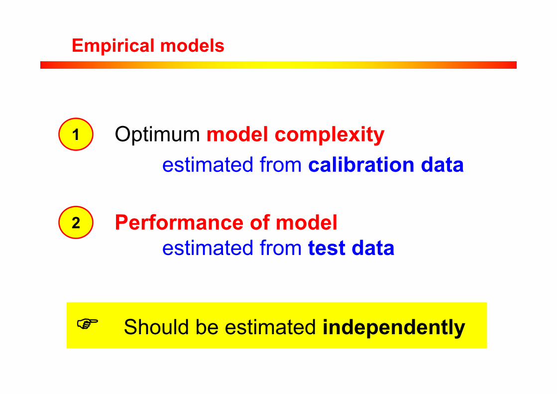
Empirical models
Performance of modelestimated from test data
2
Optimum model complexityestimated from calibration data
1
Should be estimated independently

proposed
strategy
test set
all nobjects
usuallynot many
calibrationset
estimation of optimum complexity
estimation of model performance
Repeated ! → variability of optimum complexity
→ variability of performance
n
m
→ model with (estimated)optimum complexity
Empirical models
Proposed strategy

contents
Contents1 Introduction2 Making empirical models
Calibration (OLS, PLS)Classification (DPLS, KNN)
3 Performance measuresCalibration (SEP, R2)Classification (predictive abilities)
4 StrategiesOptimum model complexityPerformance for new cases
5 Repeated double cross validationScheme - ResultsExample - Summary - Software
6 Conclusions

OLS
Multivariate calibration (linear)
trainingset
(mean-centered)
m
ni X y
b
ŷ = Xb y-ŷ
residualsm
n n
OLS
OLS Ordinary Least-Squares Regression
(yi - ŷi )2 — > min bOLS = (X TX )-1X Ty
Requirements m < n no highly correlating x-variables (columns)
No optimization of model complexity (possibly a variable selection);rarely applicable in chemistry
available data
i
only a fewselected topics

PLS
Multivariate calibration (linear)
trainingset
(mean-centered)
m
ni X y
b
ŷ = Xb y-ŷ
residualsm
n n
PLS
PLS Partial Least-Squares Regression(1) UPLS = X BPLS Intermediate, linear (latent) variables (components):
maximum covariance with y, uncorrelated or orthogonal directions in x-space, number of PLS-components is optimized
(2) OLS with UPLS
Various differentapproaches andalgorithms
simplified
applicable if m > n, applicable for highly correlating variables, optimization of model complexity !!!
available data
only a fewselected topics

regr div
Multivariate calibrationonly a few
selected topics
trainingset
(mean-centered)
m
ni X y
b
ŷ = Xb y-ŷ
residualsm
n n
?
available data
Some other regression methods in chemometrics
PCR Principal Component Regression (similar to PLS)
Lasso includes variable selection
Ridge similar to PCR (weighting of all PCA scores)
ANN Artificial Neural Networks (nonlinear)
PLS2 PLS for more than one y-variable
DPLS
Multivariate classification (linear)
trainingset
(mean-centered)
m
ni X y ŷ
correct/wrong
n n
D-PLS
available data
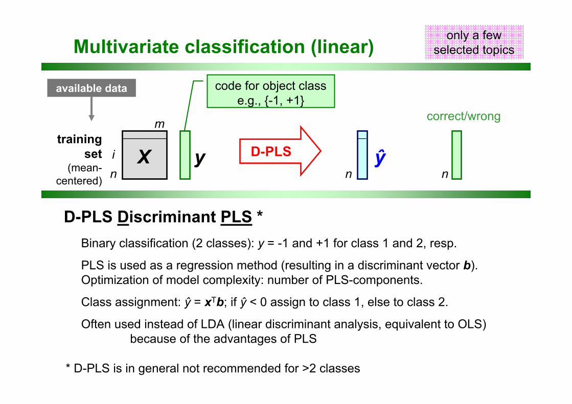
D-PLS Discriminant PLS *Binary classification (2 classes): y = -1 and +1 for class 1 and 2, resp.
PLS is used as a regression method (resulting in a discriminant vector b).Optimization of model complexity: number of PLS-components.
Class assignment: ŷ = xTb; if ŷ < 0 assign to class 1, else to class 2.
Often used instead of LDA (linear discriminant analysis, equivalent to OLS)because of the advantages of PLS
code for object classe.g., {-1, +1}
* D-PLS is in general not recommended for >2 classes
only a fewselected topics

KNN
Multivariate classification
trainingset
(mean-centered)
m
ni X y ŷ
correct/wrong
n n
KNN
available data
KNN (k-nearest neighbor) classificationAn algorithm; nonlinear; no discriminant vector.
Usually the Euclidean distance between objects (in x-space) is used to find the nearest neighbors (objects with known class membership) to a queryobject.
A majority voting among the neighbors determines the class of the queryobject.
Optimization of model complexity: k (number of neighbors)
code for object classe.g., {-1, +1}
only a fewselected topics

class div
Multivariate classification
trainingset
(mean-centered)
m
ni X y ŷ
correct/wrong
n n
?
available data code for object classe.g., {-1, +1}
Some other classification methods in chemometrics
only a fewselected topics
SVM Support Vector Machine (nonlinear)
CART Classification tree (nonlinear, evident)
SIMCA PCA models for each class (nonlinear, outlier detection)
ANN Artificial Neural Networks (nonlinear)

contents
Contents1 Introduction2 Making empirical models
Calibration (OLS, PLS)Classification (DPLS, KNN)
3 Performance measuresCalibration (SEP, R2)Classification (predictive abilities)
4 StrategiesOptimum model complexityPerformance for new cases
5 Repeated double cross validationScheme - ResultsExample - Summary - Software
6 Conclusions

meascalib
Performance measures in calibration
yi reference ("true") value for object iŷi calculated (predicted) value (test set !)ei = yi - ŷi prediction error for object i (residual)i = 1 ... z z is the number of objects used (z>n possible)
Specify: which data set (calibration set, test set) which strategy (cross validation, ...)
Distribution of prediction errors
e
bias = mean of prediction errors ei
SEP = standard deviation of prediction errors ei
= Standard Error of PredictionSEC = Standard Error of Calibration
CI = confidence interval, CI95% ≈ +2*SEP
All in units of y ! Result: ŷ + 2*SEP

meascalib
Distribution of prediction errors
e
Modeling the GC retention index (y)for n = 208 PAC by m = 467 molecular descriptors (Dragon software)
Repeated double cross validation (rdCV)with 100 repetitions (z = 20800)
m = 467; SEP = 12.7
m = 13; SEP = 8.2test set objects
yi reference ("true") value for object iŷi calculated (predicted) value (test set !)ei = yi - ŷi prediction error for object i (residual)i = 1 ... z z is the number of objects used (z>n possible)
Specify: which data set (calibration set, test set) which strategy (cross validation, ...)
Performance measures in calibration

meascalib
Predicted versus reference y's
R2 = squared (Pearson)correlation coefficient
y
ŷ
ADJ R2 = 1 - (n -1)(1-R2) / (n -m -1)squared adjusted correlation coefficientPenalizes models with a higher number of variables (m)
yi reference ("true") value for object iŷi calculated (predicted) value (test set !)ei = yi - ŷi prediction error for object i (residual)i = 1 ... z z is the number of objects used (z>n possible)
Specify: which data set (calibration set, test set) which strategy (cross validation, ...)
Performance measures in calibration
meascalib
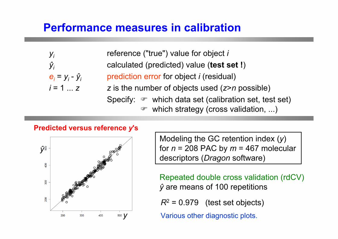
Predicted versus reference y's
ŷ
y
Modeling the GC retention index (y)for n = 208 PAC by m = 467 molecular descriptors (Dragon software)
Repeated double cross validation (rdCV)ŷ are means of 100 repetitions
R2 = 0.979 (test set objects)Various other diagnostic plots.
yi reference ("true") value for object iŷi calculated (predicted) value (test set !)ei = yi - ŷi prediction error for object i (residual)i = 1 ... z z is the number of objects used (z>n possible)
Specify: which data set (calibration set, test set) which strategy (cross validation, ...)
Performance measures in calibration

meascalib
Some other measures
(R)MSE (root) mean squared error = (root of) mean of prediction errors ei
PRESS predicted residual error = sum of squared errors eisum of squares
Q2 correlation measure for external test set objects
AIC Akaike's information criterionBIC Bayes information criterionCp Mallow's Cp
consider m
yi reference ("true") value for object iŷi calculated (predicted) value (test set !)ei = yi - ŷi prediction error for object i (residual)i = 1 ... z z is the number of objects used (z>n possible)
Specify: which data set (calibration set, test set) which strategy (cross validation, ...)
Performance measures in calibration

assigned class sum1 2
true class 1 n11 n12 n1
true class 2 n21 n22 n2
sum n→1 n→2 n
class
Class assignment table (binary classification)
Performance measures in classification
no. of objects
Predictive ability class 1 P1 = n11/n1
class 2 P2 = n22/n2
Average predictive ability P = (P1+ P2)/2
! Avoid: Overall predictive ability =(n11+ n22)/n

class
Predictive ability class 1 P1 = n11/n1
class 2 P2 = n22/n2
Average predictive ability P = (P1+ P2)/2
! Avoid: Overall predictive ability =(n11+ n22)/n
E. g.: All objects from class 1 are correctly classified;all objects from class 2 are wrong classified.Result: P1 = 1; P2 = 0; P = 0.5 (a bad classifier, OK)However, POVERALL = 0.95 ("high for a very bad classifier")
Example (warning)
n = 100; n1 = 95; n2 = 5
Performance measures in classification

measclass
Other measures for classification performance
misclassification rate for each class separatelyand summarized
risk of wrong classification different risks for wrong classification ofthe different classes can be defined
rejection rate if no assignment to any class is allowed(dead zone)
confidence of answers ratio of correct answers (assignment toa specific class 1, 2, 3, ...); depends on ration n1/n2 like overall predictive ability
Performance measures in classification
contents
Contents1 Introduction2 Making empirical models
Calibration (OLS, PLS)Classification (DPLS, KNN)
3 Performance measuresCalibration (SEP, R2)Classification (predictive abilities)
4 StrategiesOptimum model complexityPerformance for new cases
5 Repeated double cross validationScheme - ResultsExample - Summary - Software
6 Conclusions

opt complexity
Strategies (1) Optimum model complexity
fit error = 0
too high complexityof model
overfitted
error for new casesprobably large
fit error > 0
perhaps better(optimum) complexityof model
perhaps optimal fitted
error for new casesprobably smaller thanfor overfitted model
opt complexity
Strategies (1) Optimum model complexity
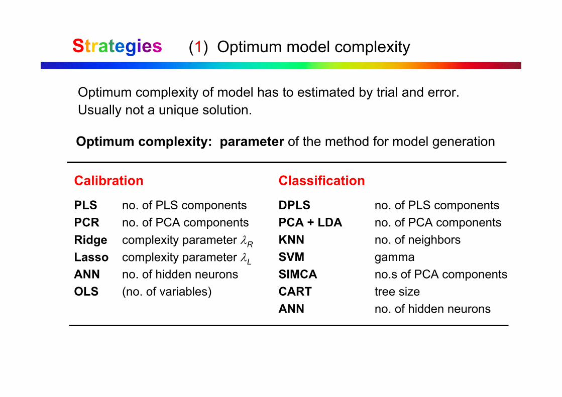
Optimum complexity of model has to estimated by trial and error.Usually not a unique solution.
Optimum complexity: parameter of the method for model generation
Classification
DPLS no. of PLS componentsPCA + LDA no. of PCA componentsKNN no. of neighborsSVM gammaSIMCA no.s of PCA componentsCART tree sizeANN no. of hidden neurons
Calibration
PLS no. of PLS componentsPCR no. of PCA componentsRidge complexity parameter R
Lasso complexity parameter L
ANN no. of hidden neurons OLS (no. of variables)

opt comple
xity
calibrationset
m
nCALIB
X y
available data
Strategies (1) Optimum model complexity
training set validation set
nTRAIN
nVAL
Split1
Make modelswith increasingcomplexity
2
. . .
Apply modelsto validation set, and store results
3
4
Results fromvalidation set(residuals,
no. of correctclassifications)
Estimate optimumcomplexity(for the given trainingset, one number)

opt complexity
Strategies (1) Optimum model complexity
Optimum model complexity: estimation, statistics
more data are better, more estimations are better
However, usual data sets (in chemistry) are small(number of objects, n = 20 ... 200)
Resampling strategies bootstrap cross validation (CV)
within a calibration set for estimation of optimum modelcomplexity (but not for estimation of model performance)
! Several estimations of the optimum complexity (distribution) !
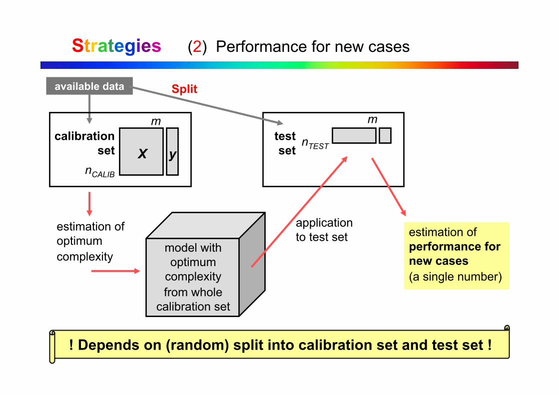
new cases
calibrationset
m
nCALIB
X y
available data
Strategies (2) Performance for new cases
nTEST
Split
mtestset
estimation of optimumcomplexity
model with optimum
complexityfrom whole
calibration set
application to test set estimation of
performance for new cases(a single number)
! Depends on (random) split into calibration set and test set !

contents
Contents1 Introduction2 Making empirical models
Calibration (OLS, PLS)Classification (DPLS, KNN)
3 Performance measuresCalibration (SEP, R2)Classification (predictive abilities)
4 StrategiesOptimum model complexityPerformance for new cases
5 Repeated double cross validationScheme - ResultsExample - Summary - Software
6 Conclusions
rdCV lit
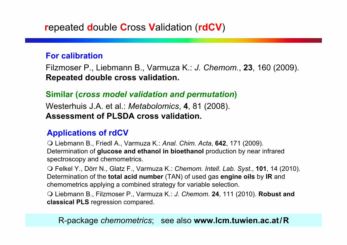
For calibrationFilzmoser P., Liebmann B., Varmuza K.: J. Chemom., 23, 160 (2009).Repeated double cross validation.
Similar (cross model validation and permutation)Westerhuis J.A. et al.: Metabolomics, 4, 81 (2008).Assessment of PLSDA cross validation.
Applications of rdCV Liebmann B., Friedl A., Varmuza K.: Anal. Chim. Acta, 642, 171 (2009). Determination of glucose and ethanol in bioethanol production by near infrared spectroscopy and chemometrics. Felkel Y., Dörr N., Glatz F., Varmuza K.: Chemom. Intell. Lab. Syst., 101, 14 (2010). Determination of the total acid number (TAN) of used gas engine oils by IR and chemometrics applying a combined strategy for variable selection. Liebmann B., Filzmoser P., Varmuza K.: J. Chemom. 24, 111 (2010). Robust and classical PLS regression compared.
R-package chemometrics; see also www.lcm.tuwien.ac.at /R
repeated double Cross Validation (rdCV)
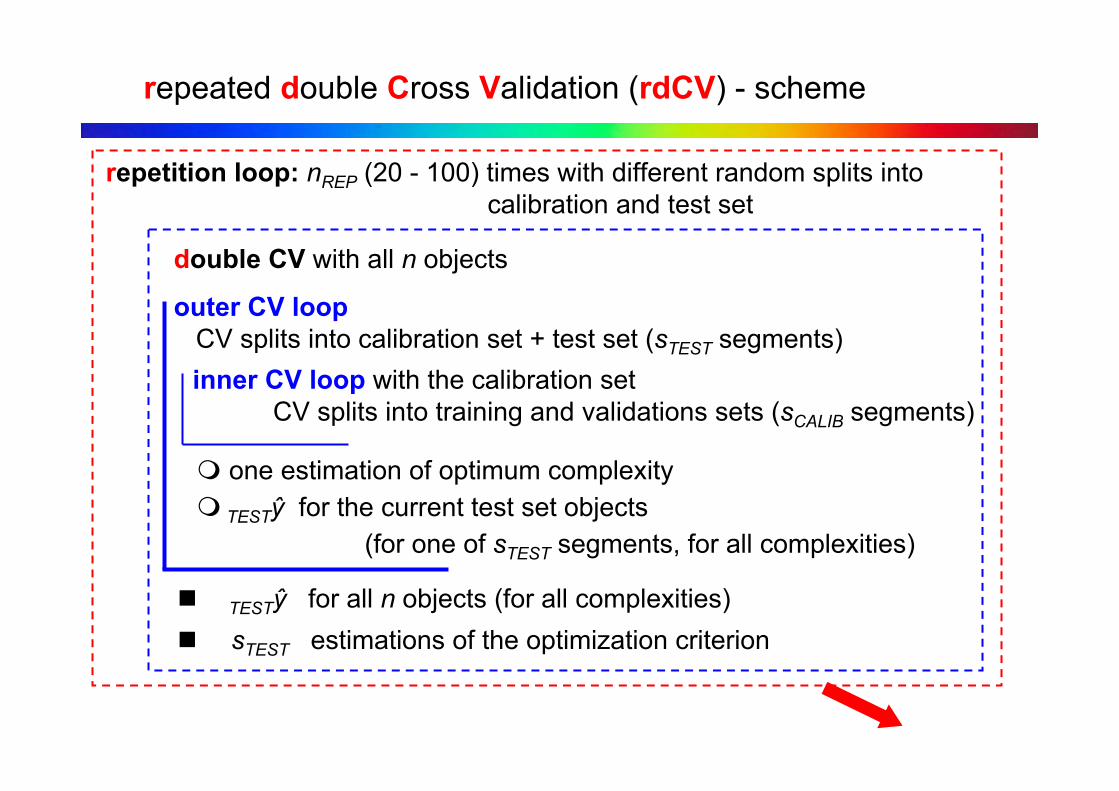
rdCVscheme
double CV with all n objects
outer CV loopCV splits into calibration set + test set (sTEST segments) inner CV loop with the calibration set
CV splits into training and validations sets (sCALIB segments)
one estimation of optimum complexity TESTŷ for the current test set objects
(for one of sTEST segments, for all complexities)
TESTŷ for all n objects (for all complexities) sTEST estimations of the optimization criterion
repetition loop: nREP (20 - 100) times with different random splits intocalibration and test set
repeated double Cross Validation (rdCV) - scheme

rdCVscheme
A
11 nREP
sTEST
estimations for optimum model complexity(all from inner CV loops with calibration sets)
test set predictions
all n objects complexities 1 ... AMAX
nREP repetitions
AFINAL
AFINAL
repeated double Cross Validation (rdCV) - results

A
1
opt complexity
sTEST * nREP values foroptimization parameter, A
1 nREP
A
frequency
Most frequent value as AFINAL
Or other heuristics, or a set of values for AFINAL( consensus model)
Typical, e. g., sTEST = 4nREP = 50give 200 estimations for the optimum complexity
sTEST
repeated double Cross Validation (rdCV) - results

A
1
opt complexity
sTEST * nREP values foroptimization parameter, A
1 nREP
A
sTEST
Modeling the GC retention index (y)for n = 208 PAC by m = 467 molecular descriptors (Dragon software).
rdCV with sTEST = 3 segments in outer loop, and nREP = 100 repetitions
frequency (300 values)
optimum no. ofPLS components;AFINAL = 11
repeated double Cross Validation (rdCV) - results

performance
test set predictions
all n objects complexities 1 ... AMAX
nREP repetitions AFINAL
nREP
n1
1
test set
predictions
repeated double Cross Validation (rdCV) - results

rperformance
nREP
n1
1
test set
predictions
SEP, R2, P, ...for the repetitions
repeated double Cross Validation (rdCV) - results

phenyl 1
mass spectrum
1 m
vector xT with spectraldescriptors (features)
Transformation:spectroscopy,mathematics,speculation
Binary classificationChemical substructure present / not present (class 1 / class 2)n = 600 (class 1: 300; class 2: 300), m = 658Dataset 'phenyl' in R-package 'chemometrics'
Werther W., Demuth W., Krueger F.R., Kissel J., Schmid E.R., Varmuza K.: J. Chemom., 16, 99 (2002)Varmuza K., Filzmoser P.: Introduction to multivariate statistical analysis in chemometrics. CRC Press,
Boca Raton, FL, USA (2009)
C6H5 -
Spectra-structure relationship (KNN, DPLS, SVM)
repeated double Cross Validation (rdCV) - example

phenyl 2
rdCV20 repetitions;sOUT = 2; sIN = 6
P (average predictive ability)
Optimized parameterKNN: kFINAL = 3DPLS: aFINAL = 2SVM: FINAL = 0.0002
Computation timeKNN 550 sDPLS 42 sSVM 940 s
Spectra-structure relationship (KNN, DPLS, SVM)
repeated double Cross Validation (rdCV) - example

rdCV summary
A resampling method combining some systematics and randomness.
For calibration and classification.
For data sets with ca ≥ 25 objects.
Optimization of model complexity (model parameter) isseparated from the estimation of model performance.
Provides estimations of the variability ofmodel complexity and of performance.
Easily applicable and fast► R-package "chemometrics"► www.lcm.tuwien.ac.at/R
repeated double Cross Validation (rdCV) - summary

rdCV PDFs
data
www.lcm.tuwien.ac.at/R
rdCV
GC-retentionindices of 206 PACs
repeated double Cross Validation (rdCV) - software

contents
Contents1 Introduction2 Making empirical models
Calibration (OLS, PLS)Classification (DPLS, KNN)
3 Performance measuresCalibration (SEP, R2)Classification (predictive abilities)
4 StrategiesOptimum model complexityPerformance for new cases
5 Repeated double cross validationScheme - ResultsExample - Summary - Software
6 Conclusions Take time and effort for validation Consider variability Accept variability and uncertainty

info & software 2 book
CRC Press, Taylor & Francis Group,Boca Raton, FL, USA, 2009ISBN: 9781420059472
Ca 320 pages,appr. € 100
Includes many R-codes (examples)However, description of methods without R
R package chemometrics
Info: www.lcm.tuwien.ac.at
Book including examples and data sets for R