evaluation of co2 fluxes from an agricultural field using a process

This article appeared in a journal published by Elsevier. The attachedcopy is furnished to the author for internal non-commercial researchand education use, including for instruction at the authors institution

and sharing with colleagues.

Other uses, including reproduction and distribution, or selling orlicensing copies, or posting to personal, institutional or third party

websites are prohibited.

In most cases authors are permitted to post their version of thearticle (e.g. in Word or Tex form) to their personal website orinstitutional repository. Authors requiring further information

regarding Elsevier’s archiving and manuscript policies areencouraged to visit:

http://www.elsevier.com/copyright

http://www.elsevier.com/copyright

Author's personal copy

Evaluation of CO2 fluxes from an agricultural fieldusing a process-based numerical model

Jens S. Buchner a,*, Jirı Simunek a, Juhwan Lee b, Dennis E. Rolston c,Jan W. Hopmans c, Amy P. King c, Johan Six b

a Department of Environmental Sciences, University of California Riverside, Riverside, CA 92521, United Statesb Department of Plant Sciences, University of California, Davis, CA 95616, United Statesc Department of Land, Air and Water Resources, University of California, Davis, CA 95616, United States

Received 28 December 2007; received in revised form 18 July 2008; accepted 23 July 2008

KEYWORDSNumerical model;Carbon dioxide;Uncertainty analysis;Soil respiration;SOILCO2;HYDRUS-1D

Summary During 2004, soil CO2 fluxes, and meteorological and soil variables were mea-sured at multiple locations in a 30-ha agricultural field in the Sacramento Valley, Califor-nia, to evaluate the effects of different tillage practices on CO2 emissions at the fieldscale. Field scale CO2 fluxes were then evaluated using the one-dimensional process-basedSOILCO2 module of the HYDRUS-1D software package. This model simulates dynamicinteractions between soil water contents, temperature, and soil respiration by numeri-cally solving partial–differential water flow (Richards) and heat and CO2 transport (con-vection–dispersion) equations using the finite element method. The model assumesthat the overall CO2 production in the soil profile is the sum of soil and plant respiration,whose optimal values are affected by time, depth, water content, temperature, and CO2

concentration in the soil profile. The effect of each variable is introduced using variousreduction functions that multiply the optimal soil CO2 production. Our results show thatthe numerical model could predict CO2 fluxes across the soil surface reasonably well usingsoil hydraulic parameters determined from textural characteristics and the HYDRUS-1Dsoftware default values for heat transport, CO2 transport and production parameters with-out any additional calibration. An uncertainty analysis was performed to quantify theeffects of input parameters and soil heterogeneity on predicted soil water contents andCO2 fluxes. Both simulated volumetric water contents and surface CO2 fluxes show a sig-nificant dependency on soil hydraulic properties.ª 2008 Elsevier B.V. All rights reserved.

0022-1694/$ - see front matter ª 2008 Elsevier B.V. All rights reserved.doi:10.1016/j.jhydrol.2008.07.035

* Corresponding author. Address: Institute of Environmental Physics, University of Heidelberg, Im Neuenheimer Feld 229, D-69120Heidelberg, Germany. Tel.: +49 175 147 40 60; fax: +49 1212 5 13058642.

E-mail addresses: [email protected] (J.S. Buchner), [email protected] (J. Simunek).

Journal of Hydrology (2008) 361, 131–143

ava i lab le a t www.sc iencedi rec t . com

journal homepage: www.elsevier .com/ locate / jhydrol


Introduction

Concerns about rising atmospheric CO2 levels and global cli-mate change have motivated the investigation of strategiesfor promoting the sequestration of C in long-term storagepools. One of these potential pools, the soil organic carbon(SOC), is affected by a variety of agricultural managementand land use strategies. Different cropping and tillage sys-tems have been shown to have a significant impact on Cdynamics (Paustian et al., 2000; Post and Kwon, 2000;McConkey et al., 2003; Osher et al., 2003).

Long-term land cultivation has contributed significantlyto the observed global warming over the last 50 years atboth the regional and global levels (IPCC, 2001, 2005). Sincesoil CO2 accumulation and respiration play a major role inthe global C cycle (Smith et al., 2003; Davidson and Jans-sens, 2006), the contribution of SOC to the entire climatesystem needs to be well understood. Different agricultural

management practices and land use have a significant im-pact on the behavior of the whole soil system and especiallyon soil C storage and greenhouse gas emissions (e.g., Paus-tian et al., 2000; Poch et al., 2005; Lee et al., 2006). Vari-ous environmental factors, such as soil temperature andwater contents, simultaneously influence the microbialmediated release of CO2 from soil C stocks (Fang and Mon-crieff, 2001; Zak et al., 1999).

Using a holistic physical approach to better understandand describe the behavior of soil systems is of major inter-est in order to predict the contribution of soils to earth’swater, CO2, chemical, and heat budgets. Of special interestfor this purpose is the one-dimensional mathematical modelSOILCO2 (Simunek and Suarez, 1993), which is built into theHYDRUS-1D software package (Simunek et al., 2005). HY-DRUS-1D simulates spatial and temporal distributions of soilwater, temperature, solutes, and CO2. Transport processesaffecting these variables are described using nonlinear

Nomenclature

Numbers in parenthesis give the equation number whenfirst used

a empirical constants (reciprocal value of the air-entry value) (cm-1)

Ad daily temperature amplitude (�C) (3)b1, b2, b3 empirical constants (soil thermal conductivity)

(J d�1 cm�2 K�1) (2)ca, cw CO2 concentration in the air and water phase

(cm3 cm�3), respectively (4)Cn, Co, Cw, Ca volumetric heat capacity of solid state, or-

ganic matter, water, and air phase, respectively(J cm�3 K�1) (2)

Das, Dws CO2 diffusion coefficients of the air and waterphase (cm2 d�1), respectively (4)

E activation energy (kg cm2 d�2 mol�1) (7)h pressure head (cm) (1)h1, h2, h3, h4, h�2, h�3 empirical constants (root water up-

take) (cm)k number of executions of SOILCO2 (9)K hydraulic conductivity (cm d�1) (1)Ks saturated hydraulic conductivity (cm d�1)KH Henry’s law constant (mol d�2 kg�1 cm�1) (4)Km Michaelis constant (–)l turtousity (–)Lb z-coordinate of the bottom of the soil profile

(cm)Lm, Lo maximum and initial rooting depth (cm), respec-

tivelyLr rooting depth (cm)Lu z-coordinate of the soil surface (cm)m number of array entries (9)n empirical constant (shape parameter) (–)N degree days to maximum production (�C)p porosity (cm3 cm�3) (4)pij random number weight factor (9)Q, Q*, S source/sink terms (d�1) (1) (4)q0 net surface flux (cm d�1)

qc, ~qc surface CO2 flux and averaged surface CO2 flux(cm3 cm�2 d�1), respectively (10)

qw water phase flux (cm d�1) (2)r empirical constant (d�1)R universal gas constant (kg cm2 d�2 K�1 mol�1)

(7)RMSD root mean square deviationt time (d) (1)td daily time (h) (3)T temperature (K) (2)T20 temperature that equals 20 �C (k) (7)Td daily average temperature (�C) (3)Tp potential transpiration rate (cm d�1)VWC volumetric water content (cm3 cm�3)y; Dy; y0 array of parameters, corresponding errors and

varied parameters, respectively (9)z z-coordinate (cm) (1)bt thermal dispersivity (cm) (2)cs0, cp0 optimal CO2 production by soil microorganism

and plant roots (cm d�1), respectively (5)g empirical constant (–) (8)hn, ho, ha volumetric fraction of solid phase, organic

matter and air phase (cm3 cm�3), respectively(2)

hw volumetric water content (cm3 cm�3) (1)hr, hs residual and saturated water contents

(cm3 cm�3), respectivelyhw; ~hw averaged (spatially and for multiple runs) water

contents (cm3 cm�3)j empirical constant (d�1) (8)kw dispersivity of the water phase (cm) (4)rhw ; �rhw standard deviation and mean standard deviation

of hw (cm3 cm�3) (11), (12)rqc ; �rqc standard deviation and mean standard deviation

of qc (cm d�1)

132 J.S. Buchner et al.


partial–differential equations. The governing transportequations, such as the Richards equation for water flowand the convection–dispersion equations for heat, solute,and CO2 transport are solved numerically using the finiteelement method. The contributions of various biologicalfactors to CO2 production (i.e., plant roots and microbiolog-ical organisms and respiration) are also considered in themodel.

The SOILCO2 model can be used for a wide range of tem-poral and spatial scales. The upper spatial limit is largelydetermined by uncertainty of input parameters due to theirspatial heterogeneity, while the lower limit is given by theminimum scale at which the governing equations are valid.While SOILCO2 can simulate short term (e.g., hourly or dai-ly) CO2 variations, the large majority of models simulating Cand N turnover in soils, such as the DNDC (Li et al., 1992),CANDY (Franko et al., 1997), CENTURY (Parton et al.,1987, 1988, 1993), and RothC (Coleman and Jenkinson,2005) are based on mass balance equations for finite soillayers and are designed for large spatial and long temporalscales. This enhances the applicability of these models inregional and global models but limits their use for studiesof local processes. Recently, the SOILCO2 model has re-ceived increased attention, and several of its applicationshave appeared in recent studies. For example, Herbstet al. (2008) coupled the SOILCO2 model with a carbon turn-over model and then successfully used the coupled model tosimulate multiyear heterotrophic soil respiration from abare soil experimental plot in Germany. Bauer et al.(2008) evaluated the sensitivity of simulated soil heterotro-phic respiration to varying temperature and moisture reduc-tion functions implemented in SOILCO2.

In this paper, we evaluate soil CO2 emissions from agri-cultural soils in the Sacramento Valley, California, usinglimited meteorological and soil information, and the one-dimensional process-based SOILCO2 module of the HY-DRUS-1D software package. The major objective of ourinvestigations was to evaluate the performance of the SOIL-CO2 model using typically collected information. Since mea-surements were not collected specifically for our model,both measured soil properties and literature values wereused to parameterize the model. To quantitatively evaluatethe impact of uncertainties of measured soil properties, arandom value uncertainty analysis was carried out. Suchanalysis shows the capabilities and limits of the model, gi-ven its large demand on information and the one-dimen-sional representation of the soil domain.

Methods

Site description and data sampling

The experimental site is a 30-ha furrow irrigated agricul-tural field, located in the Sacramento Valley, near Winters,CA (38�36 N, 121�50 E). The slope of the field is less than 2%.The site was under observation using biweekly (growing sea-son) and monthly (non-growing season) measurements ofCO2 emission, soil temperature, and volumetric water con-tent during the period from 2003 until the middle of 2006for predicting changes in landscape-scale soil organic C ina field recently converted from standard to minimum tillage

(Poch et al., 2005; Lee et al., 2006, 2007). The tillage andcropping history of the site was described in detail by Leeet al. (2007). In short, the field had been divided into twoequal-sized areas in October 2003, and these were farmedusing standard and minimum tillage. From April until Sep-tember 2004, the field was cultivated with maize (Zea maysL.). For the modeling study presented in this paper, thetime period from January 1 until December 31, 2004 wasused.

Measurements of CO2 emissions and relevant physicalvariables, such as precipitation, potential evaporation, airtemperature, and volumetric water contents were carriedout during this period. Figs. 1 and 2 present measureddaily values of precipitation, irrigation, potential evapo-transpiration, and air temperature. Meteorological datawere obtained from the California Irrigation ManagementInformation System CIMIS (http://wwwcimis.water.ca.gov/).

In 2003, 30 plots for sampling of gases were establishedin the field. Two types of non-steady-state portable cham-bers that cover the soil surface only (no plants) were used.Insulated stainless steel chambers, which we moved fromsite to site and covered 0.012 m2 of soil surface, were usedfrom September 2003 through April 2004. In May 2004,0.051 m2 PVC rings were installed in the field. The rings

0 100 200 300

Time [d]

Inpu

t [m

m]

Precipitation Irrigation Evapotranspiration90

60

30

0

-3

-6

-9

-12

Figure 1 Mean daily values of precipitation, irrigation, andevapotranspiration. Please note the different scales for positiveand negative values.

0

5

10

15

20

25

30

0 100 200 300

Time [d]

Tem

pera

ture

[˚C

]

Figure 2 Mean daily (full line) and average annual (dottedline) air temperatures.

Evaluation of CO2 fluxes from an agricultural field using a process-based numerical model 133


were pushed approximately 5 cm into the soil and placed atfour different spots: the middle of the bed, the middle ofthe furrow, over the crop row but between plants (whenapplicable), and over the side dressed band (when applica-ble). Portable PVC end caps were converted into chamberlids, and placed on top of the rings for sampling. The CO2

concentration inside the chambers was measured at 0, 30,60, 120, 180, 240, and 300 s after placement of chambersover the soil surface with a Licor 6262 IRGA. The soil CO2

flux was calculated using the measured CO2 concentrationsas input in the non-steady-state diffusive flux estimatormodel (Livingston et al., 2005, 2006). Measurements weretaken at different times of the day at different locations.Since Lee et al. (2006) found little or no differences be-tween CO2 emissions from parts of the field with standardand minimum tillage, measurements from both sides ofthe field were combined in our analyses.

During each gas flux sampling, volumetric water contentwas measured using a portable time domain reflectometeryprobe (HydroSense, Decagon Devices Inc., Pullman, WA)over a depth interval from 0 to 12 cm. A field-specific cali-bration curve was generated using a polynomial regressionof probe values to volumetric water contents (determinedgravimetrically) for the top 0–12 cm.

Lee et al. (2007) also collected soil samples for measure-ments of soil texture in August 2003 (Table 1). The measure-ments were taken at 140 points in five depths (0–15, 15–30,30–50, 50–75, and 75–100 cm). Bulk density, clay, silt, andloam percentages were averaged over all locations for aparticular depth, as well as over the entire soil profile (Ta-ble 1). According to the USDA textural classification system,the soil can be categorized as being almost exactly on theboundary between loam and silt loam (Soil ConservationService, 1972). The relatively large standard deviations re-flect the high spatial variability of the measured soil physi-cal properties across the field.

Numerical model

The SOILCO2 model (Simunek and Suarez, 1993; Simuneket al., 2005) numerically simulates the movement of water,solutes, heat, and CO2 in an arbitrary one-dimensional soildomain. The soil domain is represented by a spatial grid,in which every point can be assigned a certain soil type.Therefore, all functions representing physical variablescan depend on both z and t, where z (cm) is the Euclidiancoordinate orthogonal to the soil surface, and t (d) is time.The z-coordinate of the top and bottom of the soil column

are designated as Lu and Lb, respectively. The followingdescription follows the work of Simunek and Suarez(1993). Note the notation section for definitions of variousparameters.

Water movementWater movement in a partially-saturated rigid porous med-ium, where the air phase is considered to be under constantatmospheric pressure, can be described using the followingform of the Richards’ equation:

ohw

ot¼ o

ozK

oh

oz� 1

� �� Q ð1Þ

where hw(h,z,t) is the volumetric water content(cm3 cm�3), K(h,z,t) is the hydraulic conductivity (cm d�1),h(z,t) is the pressure head (cm), and Q(h,z,t) is the rootwater uptake (d�1). The two functions hwðhÞ and K(h) canbe described using the van Genuchten model (van Genuch-ten, 1980). These relations define soil hydraulic propertiesusing six soil hydraulic parameters: residual water contenthr, saturated water content hs, shape parameters a and n,saturated hydraulic conductivity Ks, and tortuosity andpore-connectivity parameter l.

The root water uptake function Q(h,z,t) in Eq. (1) is aproduct of the potential transpiration rate Tp(t) (cm d�1),the function b(z) (cm�1) characterizing the spatial distribu-tion of the root water uptake (Simunek et al., 2005), andthe stress response function a(h). The time-dependent root-ing depth, Lr, which affects the b(z) function, is describedusing the Verhulst–Pearl growth function (Simunek andSuarez, 1993). The stress response function a(h) is definedfollowing Feddes et al. (1978) using four empirical constantsh1, h2, h3, and h4 (cm) that characterize optimality of theroot water uptake. The plant root water uptake model istherefore characterized by parameters Tp, Lm, L0, h1, h2,h3, and h4.

Atmospheric and free drainage boundary conditions areused at the upper and lower boundaries, respectively.

Heat transportHeat transport can be described using the following convec-tion–dispersion equation when the effects of the water va-por diffusion are neglected:

ðCnhn þ Coho þ Cwhw þ CahaÞoT

ot

¼ o

ozb1 þ b2hw þ b3h

0:5w þ btCwjqwj

� � oT

oz

� �� Cwqw

oT

ozð2Þ

Table 1 Percentages of clay, silt, and sand, bulk density (BD) and organic carbon content (Corg) for individual soil horizonsaveraged over all locations, as well as their average over the entire soil profile

Depth (cm) Clay (%) Silt (%) Sand (%) BD (g cm�3) Corg (g m�3)

0–15 17.1 ± 3.1 51.5 ± 6.0 31.4 ± 8.7 1.04 ± 0.06 1220 ± 17815–30 18.9 ± 3.4 53.5 ± 6.6 27.6 ± 9.6 1.37 ± 0.08 1215 ± 23330–50 20.8 ± 3.7 52.8 ± 7.9 26.4 ± 10.1 1.51 ± 0.07 1025 ± 24850–75 20.0 ± 4.1 51.7 ± 9.9 28.2 ± 13.4 1.58 ± 0.01 1092 ± 31075–100 19.1 ± 4.4 48.3 ± 11.4 32.7 ± 15.16 1.58 ± 0.01 680 ± 3570–100 19.3 ± 3.8 51.3 ± 8.8 29.4 ± 12.0 1.46 ± 0.04 1083 ± 311

Standard deviations of measured values are given after the ‘±’ symbol. Measurements were taken in August 2003.



where Ci (J cm�3 K�1) and hi (z,t) (cm

3 cm�3) are volumetricheat capacities and volumetric fractions, respectively. Thesubscripts n, o, w, and a represent the mineral phase, or-ganic matter, liquid phase, and air phase, respectively. InEq. (2), T (z,t) (K) and qw (cm d�1) represent temperatureand water phase flux, respectively; b1, b2, and b3(J d�1 cm�1 K�1) are empirical constants used in the func-tion describing the dependency of the thermal conductivityon hw, and bt (cm) is the thermal dispersivity. Hence, thesoil thermal parameters Cn, Co, Cw, Ca, ho, hn, b1, b2, b3,and bt characterize the heat transport process.

Similarly as for water flow, the initial condition is givenas the spatial temperature field T(z) at t = 0 d. The upperboundary condition is specified as a Dirichlet boundary con-dition using the following sinusoidal function to representdaily variations of temperature at the soil surface:

TðtdÞ ¼ TdðtÞ þ AdðtÞ sin2ptdtp� 7p

12

� �; z ¼ Lu ð3Þ

Here, Td (t) (�C), Ad(t) (�C), td (h), and tp (=24 h) stand forthe daily average temperature, daily temperature ampli-tude, day time, and day length, respectively. A Dirichletboundary condition representing the annual average airtemperature was used at the lower boundary.

Transport and production of carbon dioxideIn SOILCO2, CO2 transport is assumed to be caused by con-vection in the liquid phase, and diffusion in both the liquidand air phases. Furthermore, the gas phase is assumed to bestagnant, and the interaction of CO2 with the soil matrix isneglected. The CO2 concentrations in the water phase, cw(cm3 cm�3), and in the air phase, ca (cm

3 cm�3), are linkedusing Henry’s law (Simunek and Suarez, 1993).

The following convection–dispersion equation can thenbe used to describe the CO2 transport:

oðcaha þ cwhwÞot

¼ o

ozhaDas

h7=3a

p2

!ocaozþ hw Dws

h7=3w

p2þ kw

qw

hw

��

!ocwoz

" #

� o

ozðqwcwÞ � Q � þ S ð4Þ

where ha and hw (cm3 cm�3) are the volumetric contents ofair and water phase, respectively, Das and Dws (cm

2 d�1) arethe diffusion coefficients of CO2 in the gas and dissolvedphases, respectively; p (cm3 cm�3) is the porosity and kw(cm) is the dispersivity in the water phase. The termsQ*(z,t) (cm3 cm�3 d�1) and S (z,t) (cm3 cm�3 d�1) representthe sink/source terms for dissolved CO2 in root water uptakeand the CO2 production by microorganisms and plant roots,respectively. The latter term is an important term of Eq.(4), as the CO2 budget in the soil profile strongly dependson it. While volumetric water and air contents are expressedin units of volume of a particular phase divided by the vol-ume of soil, CO2 concentrations are defined in units of theCO2 volume divided by the volume of the liquid or gas phase,respectively.

Initial conditions have to be provided for CO2 concentra-tions, i.e., ca(z) at t = 0, similar to those for pressure headsand temperatures. The Dirichlet boundary condition with caequal to the atmospheric CO2 concentration (=0.000379),

(IPCC, 2005) was used at the soil surface (z = Lu). At the low-er boundary, a von Neumann boundary condition with zeroconcentration gradient was used since we expect a verylow variability of the CO2 concentration at the lowerboundary.

The SOILCO2 model assumes that CO2 is produced by soilmicroorganism and plant roots, and that these two pro-cesses are additive (Simunek and Suarez, 1993). The modelfurther assumes that the CO2 production depends on severalphysical factors, and that the effect of these factors can berepresented using the multiplication of appropriate func-tions. Hence,

S ¼ cs0Yi

fsi þ cp0Yi

fpi ð5Þ

Yi

fi ¼ fðzÞfðhÞfðTÞfðcaÞfðtÞ ð6Þ

where subscripts s and p refer to soil microorganism andplant roots, respectively, cs0 and cp0 (cm3 cm�2 d�1, i.e.,volume of CO2 per unit area of the soil surface per unit time)are the optimal CO2 production rates and f are individualreduction functions representing influence of various envi-ronmental factors.

Simunek and Suarez (1993) and Suarez and Simunek(1993) provided detailed description of all reduction func-tions used in Eqs. (5) and (6). But to further emphasizethe importance of the temperature dependence of theCO2 production, we give here only f(t), which is assumedto be described by the Arhenius equation as follows

fðTÞ ¼ expEðT � T20ÞRT T20

� �ð7Þ

where E (kg cm2 d�2 mol�1) is the activation energy of thereaction, on which CO2 production is based, R (kg cm2

d�2 K�1 mol�1) is the universal gas constant, and T20(=293.15 K or 20 �C) is the reference temperature for theoptimal production. It should be noted that from all reduc-tion functions (6) only the function (7) can have values lar-ger than one (for T > T20) and thus an especially stronginfluence of the soil temperature on the CO2 production isexpected for these temperatures.

In summary, the transport of CO2 is characterized fullyby the set of transport parameters Das, Dws, and kw andthe set of production parameters cs0, cp0, N, E, Km, a*, h

�2,

and h�3 (see the Notation section for definitions). The defaultparameters discussed in Suarez and Simunek (1993) wereused in the following simulations unless mentionedotherwise.

Selection of parameters, boundary and initialconditions

Proper selection of model parameters, characterizing dif-ferent transport processes and factors, is of particularimportance for the performance of the model and its sim-ulation results. Whenever possible, the selection shouldbe made based on measured data. However, when mea-sured data have not been collected specifically for a par-ticular model (the SOILCO2 model in this case), externalsources need to be used instead. The following section



discusses the set-up of the SOILCO2 model for this partic-ular application and how required input parameters wereobtained.

The 100-cm deep transport domain was described using aone-dimensional soil column with a spatial resolution of1 cm. Two different ways were used to obtain the soilhydraulic parameters. First, the Rosetta module (Schaapet al., 2001) was applied using the data listed in Table 1and assuming a vertically homogeneous soil profile. Second,average soil hydraulic parameters (Carsel and Parrish, 1988)were used for the soil textural classes classified according tothe USDA system. Since the soil texture was categorized asalmost exactly on the boundary between loam and silt loam,calculations were carried out using both textural classes.Three different sets of the soil hydraulic parameters andthe corresponding retention curves are presented in Table2 and Fig. 3, respectively.

The CIMIS data provides only potential evapotranspira-tion rates, ET0, which need to be divided into potentialevaporation and potential transpiration rates for use in HY-DRUS-1D. Therefore, the following logistic growth approachwas used for this purpose:

TpðtÞ ¼ ET0ðtÞg

gþ ð1� gÞ expð�jtÞ ð8Þ

where Tp is the potential transpiration (cm d�1). The twoempirical parameters (g = 0.0001 and j = 0.193 d�1) wereevaluated assuming that transpiration is, on average, 75%

of evapotranspiration during the entire growth period(Zhang et al., 2000). The evaporation rate is then given asa complementary value (Fig. 4). Since maize was plantedin April, L0 was set equal to zero. Dwyer et al. (1995) foundmaize’s maximum rooting depth Lm to be 90 cm. The atmo-spheric boundary conditions are shown in Figs. 1 and 4.

Since no measurements of soil thermal parameters werecarried out in the studied field, we used the default valuesof thermal capacities for individual soil phases, and thethermal conductivity function for silt, the dominant tex-tural fraction (see Table 1). Soil thermal parameters usedin HYDRUS-1D simulations are given in Table 3.

The upper boundary condition for heat transport calcu-lations is defined for daily time td using average daily airtemperatures, Td(t) (Fig. 2), and daily temperature ampli-tudes, Ad(t) (Eq. (3)). Because of the lack of informationabout the bottom boundary, we used the mean air tem-perature, T = 15.4 �C, as the constant bottom boundarycondition.

A comprehensive review of the selection of values foroptimal CO2 production, as well as coefficients for particu-lar reduction functions, was provided by Suarez and Simu-nek (1993). The values for different reduction coefficientsand optimal CO2 production rates suggested in this review,which are implemented as default values in the HYDRUS-1D software package (Simunek et al., 2005), were used inthe CO2 transport and production model (Eqs. (5)–(7)).These coefficients, as well as coefficients describing rootwater uptake, are given in Table 3.

Since there were no specific measurements of initial con-ditions for h(z), T(z), and c(z), we assumed a hydrostaticequilibrium for h(z), and constant values for T(z) = 15.4 �Cand c(z) = 0.000379 cm3 cm�3.

Table 2 Soil hydraulic parameters determined using different methods: (A) neural network prediction using Rosetta (Schaapet al., 2001), (B) average parameters for the silt loam textural class (Carsel and Parrish, 1988), and (C) average parameters forthe loam textural class (Carsel and Parrish, 1988)

Method hr (cm3 cm�3) hs (cm

3 cm�3) a (cm�1) n Ks (cm d�1) l

A 0.062 0.386 0.007 1.59 11.28 �0.036B 0.067 0.450 0.020 1.41 10.80 0.500C 0.078 0.430 0.036 1.56 24.96 0.500

0

1

2

3

4

5

6

0 0.1 0.2 0.3 0.4 0.5VWC [cm3 cm-3]

log1

0(h

[cm

])

A B C

Figure 3 Retention curves corresponding to soil hydraulicparameters presented in Table 2. These parameters wereobtained using (A) neural network predictions with Rosetta(Schaap et al., 2001), (B) average parameters for the silt loamtextural class (Carsel and Parrish, 1988), and (C) averageparameters for the loam textural class (Carsel and Parrish,1988). VWC – volumetric water content.

0

2

4

6

8

10

12

0 100 200 300Time [d]

Eva

p. &

Tra

nsp.

[m

m]

Figure 4 Mean daily values of potential evaporation (blackline) and potential transpiration (grey line) during the simula-tion period.



Parameter variation

As mentioned above, hydraulic properties and heat trans-port parameters were chosen or calculated based on the soiltexture presented in Table 1. Large spatial variability of soiltextural parameters produces uncertainty in predictedtransport parameters, and consequently in model predic-tions. To evaluate the influence of this uncertainty on mod-eling results and study model sensitivity to theseparameters, an uncertainty analysis was carried out.

For each parameter set, we defined an array y of se-lected input parameters and an associated array of errorsDy (Table 4), whereby each array consists of m entries.For each entry j, Dyj is defined such that 2Dyj matchesthe whole error range. While in section Model perfor-mance’, the model is executed with only one array y, inthe uncertainty analysis the model is executed a sufficientnumber of times (k) with the modified array y0 to evaluatethe model sensitivity to a particular parameter. The sub-script i indicates each execution. The entries j of this arrayare given by

y 0ij ¼ yj þ pijDyj 8j 2 f0; . . . ;mg ^ i 2 f0; . . . ; kg ð9Þ

Weight factors pij (–) are normally distributed random num-bers (Press et al., 1992) with a standard deviation that isequal to unity.

For the uncertainty analysis, the following quantitieswere defined. Averaging of simulated CO2 fluxes, qci(0,t)(cm3 cm�2 d�1), over all executions i gives mean CO2 fluxes~qc (cm3 cm�2 d�1) and their corresponding standard devia-tions rqc (cm3 cm�2 d�1):

~qcð0; tÞ ¼ k�1Xki¼0

qcið0; tÞ ð10Þ

rqcð0; tÞ ¼

ffiffiffiffiffiffiffiffiffiffiffiffiffiffiffiffiffiffiffiffiffiffiffiffiffiffiffiffiffiffiffiffiffiffiffiffiffiffiffiffiffiffiffiffiffiffiffiffiffiffiffiffiffiffiffiffiffiffiffiffiffiffiffiffiffiffiffiffiðk� 1Þ�1

Xki¼0½qcið0; tÞ � ~qcð0; tÞ�2

vuut ð11Þ

The mean standard deviation �rqc (cm3 cm�2 d�1) is obtained

by averaging standard deviations rqc over the simulationperiod as follows:

�rqcð0Þ ¼ ðt2 � t1Þ�1Z t2

t1

rqcð0; tÞdt ð12Þ

where t1 and t2 are the beginning time (=1 d) and the endingtime (=366 d) of the simulation.

Table 4 Parameters and corresponding standard deviations used in the uncertainty analysis

hr (cm3 cm�3) hs (cm

3 cm�3) a (cm�1) n Ks (cm d�1) l0.067 0.40 0.007 1.59 11.37 �0.044Dhr (cm

3 cm�3) Dhs (cm3 cm�3) Da (cm�1) Dn DKs (cm d�1) Dl

0.008 0.02 0.001 0.04 3.87 0.128

b1 (J s�1 m�2 K�1) b2 (J s�1 m�2 K�1) b3 (J s�1 m�2 K�1)0.154 �0.784 2714Db1 (J s�1 m�2 K�1) Db2 (J s�1 m�2 K�1) Db3 (J s�1 m�2 K�1)0.035 0.333 612

Upper and lower four rows show hydraulic and selected thermal properties, respectively.

Table 3 Parameters used in the model. Superscript numbers indicate literature source: (1) Taylor and Ashcroft (1972), (2)Chung and Horton (1987), (3) Patwardhan et al. (1988), (4) Suarez and Simunek (1993), (5) Holt et al. (1990), (6)www.wikipedia.org, (7) Simunek et al. (2005), (8) Maas (1990), (9) Buyanovski et al. (1986), and (10) Williams et al. (1972)

Root water uptake parametersh1 (cm)1 h2 (cm)1 h3u (cm)1 h3l (cm)1 h4 (cm)1

�15 �30 �325 �600 �8000

Heat transport parametersCn (J m�3 K�1)2 Co (J m�3 K�1)2 Cw (J m�3 K�1)2 Ca (J m�3 K�1)2

1.92 · 106 2.51 · 106 4.18 · 106 1.250 · 103

b1 (J s�1 m�2 K�1)2 b2 (J s�1 m�2 K�1)2 b3 (J s�1 m�2 K�1)2 bt (m)2

0.243 0.393 1.534 0.05

CO2 production parametersDas (cm

2 d�1)3 Dws (cm2 d�1)3 kw (m) p (cm3 cm�3) cs0 (cm3 cm�2 d�1)4

1.37376 · 104 1.529 Equal to bt Equal to hs 0.42

cp0 (cm3 cm�2 d�1)5 N (�C)6 Ep (kg cm2 d�2 mol�1)7 Es (kg cm2 d�2 mol�1)8

0.28 1360 6.48 · 1017 7.19 · 1017

K�4m a (cm�1)9 h�2 (cm)10 h�3 (cm)10

0.14 0.105 �100 �106



Similar definitions as those used for CO2 fluxes in thethree equations above, were also used for the volumetricwater contents, hi(0,t).

Mean hydraulic parameters and their corresponding stan-dard deviations used in the uncertainty analysis (Table 4)were obtained using the Rosetta model (Schaap et al.,2001) in combination with soil textural measurements (Ta-ble 1). Using mean values and standard deviations of thepercentages of sand, silt, and clay, and bulk density (Table1), new values of these variables were sampled 1000 timesassuming that they are normally distributed. A new set ofthe soil hydraulic parameters was estimated using Rosettafor each new set of textural properties. These new setswere then evaluated to get their statistical parameters. Thismethod, however, leads to a maximum coefficient of varia-tions of 30% for Ks. This is small compared to the coefficientof variations of 120% reported by Nielsen et al. (1973).Hence, this latter value was used in the uncertainty analysis(Table 4) instead of the value provided by Rosetta. Meanvalues of the hydraulic parameters, and their correspondingstandard deviations, presented in Table 4 are the result ofthese estimates.

A different method was used for soil thermal parame-ters. Chung and Horton (1987) provided thermal parametersonly for clay, silt, and sand. While in direct calculations weused thermal parameters for silt, since silt is the main tex-tural fraction, for the uncertainty analysis we calculatedweighted averages and standard deviations of the threethermal parameters (Table 4) using the textural fractions(Table 1) as weighting.

3. Results and discussion

Model performance

Three simulation runs were performed with soil hydraulicproperties obtained using the different methods (Table 2).Below, we present model results for the surface CO2 flux,qc(0,t) (cm3 cm�2 d�1) and the volumetric water contentaveraged over the surface soil layer of 12 cm thickness:

hwðtÞ ¼ 1�1Z 1

0

hwðz; tÞdz ð13Þ

Here, hw(z,t) (–) is the volumetric water content as a func-tion of depth and time, and 1 = 12 cm.

Fig. 5 shows a comparison of spatially averaged mea-sured and calculated volumetric water contents for thethree different sets of soil hydraulic parameters, listed inTable 2. In general, higher water content values were mea-sured after rainfall or irrigation events, while high potentialevapotranspiration resulted in a decrease in water contentsduring time periods without precipitation or irrigation. Asexpected, simulated water contents depended mainly onclimatic conditions for all three runs. Rainfall events (Fig.1) and low potential evapotranspiration rates (Fig. 4) ledto high soil water contents in the range of 0.18–0.38 cm3 cm�3 from day 0 to day 70. Light precipitationand increasing potential evapotranspiration rates led to val-ues in the range of 0.10–0.25 cm3 cm�3 between days 70and 250. Only irrigation events during the same time periodled to higher water contents for short times. In the last time

period (after day 250), moderate precipitation and decreas-ing evapotranspiration rates resulted in water contents inthe range of 0.27–0.30 cm3 cm�3. Measured values are dis-played with fairly large errors, indicating a high spatial var-iability across the field.

In all three runs, simulated values were in the samerange as measured values. In run A, 32.5% of simulated val-ues were in the error range of measured ones, while in runsB and C, 50.0% and 27.5% were in this range, respectively.Root mean square deviations (RMSD) were found to be0.11, 0.07, and 0.09 cm3 cm�3, for A, B, and C, respectively.In addition, we observed coefficients of correlation of 0.19,0.23, and 0.26. The best model performance was found forscenario B. The coefficients of correlation indicate a signif-icant discrepancy between the modeled and measured val-ues. The relative error of the water mass balance formodel calculations was 0.076%, 0.102%, and 0.106% for caseA, B, and C, respectively.

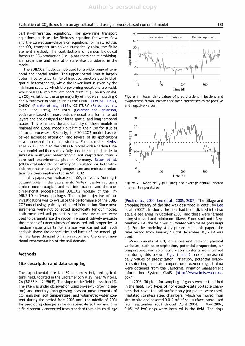
Fig. 6 presents measured and simulated soil tempera-tures at a depth of 5 cm. Simulation results for run A, B,and C were almost identical and thus are represented inthe figure by a single line. Simulated values (31.6%) werein the error range of measured ones. The root mean squaredeviation (RMSD) and the coefficient of correlation werefound to be 3.27�K and 0.90, respectively. Although theseresults and Fig. 6 show that the model can very well de-

0

0.1

0.2

0.3

0.4

0.5

0 100 200 300

0 100 200 300

VW

C [

cm 3 cm

-3]

measured A B C

-0.2

-0.1

0

0.1

0.2

0.3

Time [d]

Res

idu

al V

WC

[cm

3 cm

-3]

A B C

Figure 5 Measured and simulated volumetric water contents(VWC) (cm3 cm�3) averaged over the top soil layer at meandaily measurement times (top). Error bars represent onestandard deviation resulting from spatial averaging. Residual(measured minus modeled) volumetric water contents (bot-tom). Cases A, B, and C are the same as in Fig. 3.



scribe the overall annual trend of soil temperatures, thereare some differences for particular measurement times.There can be several reasons for this. Measurements acrossthe entire field were taken over several hours (similarly aswater contents) and then averaged. Measurements weretaken with a digital thermistor at a 5-cm depth every timeCO2 flux measurements were taken and thus measurementdepths and locations may have varied. Both these factorscan lead to relatively unreliable values of measuredtemperatures.

Measured and simulated CO2 fluxes as a function of timeare presented in Fig. 7. There is one significant outlier mea-sured at day 79, likely caused by a measurement error. TheCO2 efflux appears to display the same annual trend as airtemperatures (Fig. 2), with the exception of the time periodfrom day 100 to 150. This is likely due to low water contentsduring this time period, which led to reduction of soil CO2

fluxes. High error ranges of CO2 fluxes are partly due to ahigh spatial variability of water content values and partlydue to different measurement times. Since measurementsat different spots were typically taken during a time intervalof 3 h, significant temperature differences could be ob-served between measurements at different locations. Wealso expect that there is a small contribution by the two

different tillage practices to the high variability of observedCO2 fluxes (Lee et al., 2006).

The correspondence between measured and simulatedCO2 fluxes was relatively good for all three simulation runs.Simulated values are within the error range of measuredvalues in 80.0%, 77.5%, and 75% of cases for scenario A, B,and C, respectively. The large difference between mea-sured and simulated CO2 fluxes at day 295 is likely causedby the underestimation of the water content at the sametime (Fig. 5).

A comparison of measured and simulated CO2 fluxes (Fig.7) with air temperatures (Fig. 2) shows the trend in the CO2

efflux (using Eq. (7)) follows the annual temperature trend.Furthermore, irrigation events on days 133, 157, 170, 179,196, 210, and 228 led to higher water contents, whichshould not limit CO2 production by soil microorganisms.However, the CO2 production by plant roots has beenparameterized by the Feddes et al. (1978) function. Sinceirrigation events increase pressure heads (water contents)beyond their optimal range, the CO2 production by plantroots decreases and so does the overall CO2 production, be-cause of the additive approach given by Eq. (5).

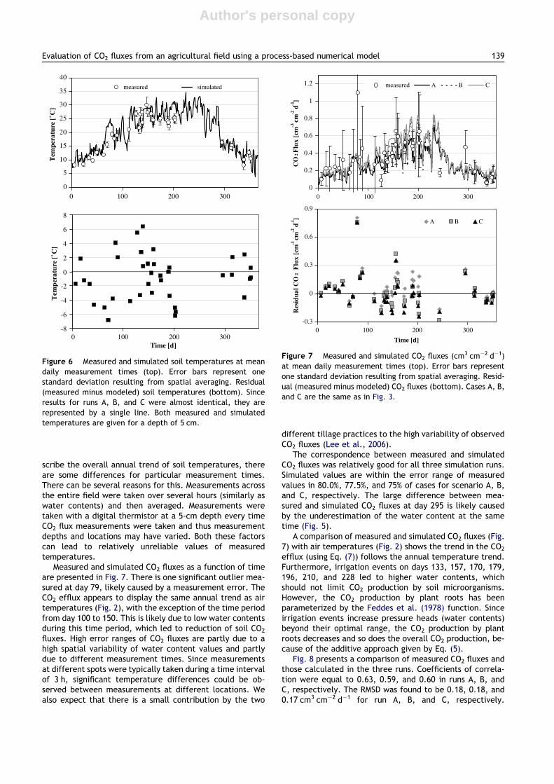
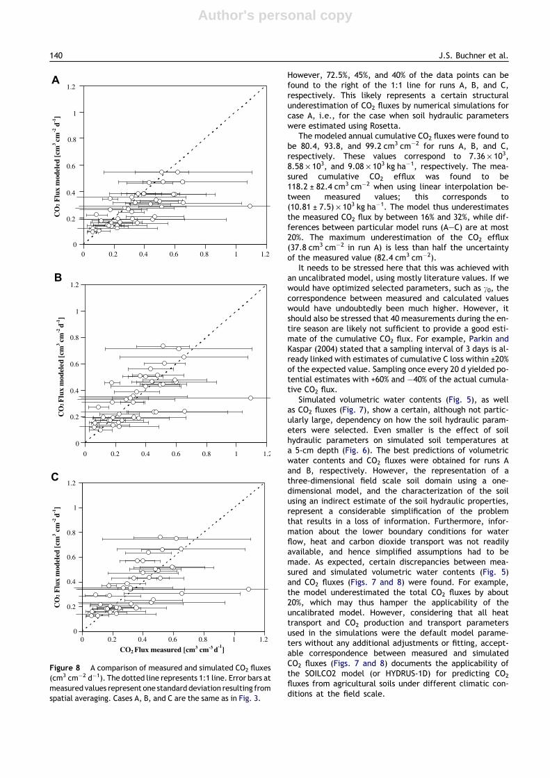
Fig. 8 presents a comparison of measured CO2 fluxes andthose calculated in the three runs. Coefficients of correla-tion were equal to 0.63, 0.59, and 0.60 in runs A, B, andC, respectively. The RMSD was found to be 0.18, 0.18, and0.17 cm3 cm�2 d�1 for run A, B, and C, respectively.

0

5

10

15

20

25

30

35

40

0 100 200 300

Tem

pera

ture

[˚C

]

measured simulated

-8

-6

-4

-2

0

2

4

6

8

0 100 200 300Time [d]

Tem

pera

ture

[˚C

]

Figure 6 Measured and simulated soil temperatures at meandaily measurement times (top). Error bars represent onestandard deviation resulting from spatial averaging. Residual(measured minus modeled) soil temperatures (bottom). Sinceresults for runs A, B, and C were almost identical, they arerepresented by a single line. Both measured and simulatedtemperatures are given for a depth of 5 cm.

0

0.2

0.4

0.6

0.8

1

1.2

0 100 200 300

CO

2 F

lux

[cm

-3 cm

-2 d

-1]

measured A B C

-0.3

0

0.3

0.6

0.9

0 100 200 300

Time [d]

Res

idua

l CO

2 F

lux

[cm

-3 cm

-2 d

-1] A B C

Figure 7 Measured and simulated CO2 fluxes (cm3 cm�2 d�1)at mean daily measurement times (top). Error bars representone standard deviation resulting from spatial averaging. Resid-ual (measured minus modeled) CO2 fluxes (bottom). Cases A, B,and C are the same as in Fig. 3.



However, 72.5%, 45%, and 40% of the data points can befound to the right of the 1:1 line for runs A, B, and C,respectively. This likely represents a certain structuralunderestimation of CO2 fluxes by numerical simulations forcase A, i.e., for the case when soil hydraulic parameterswere estimated using Rosetta.

The modeled annual cumulative CO2 fluxes were found tobe 80.4, 93.8, and 99.2 cm3 cm�2 for runs A, B, and C,respectively. These values correspond to 7.36 · 103,8.58 · 103, and 9.08 · 103 kg ha�1, respectively. The mea-sured cumulative CO2 efflux was found to be118.2 ± 82.4 cm3 cm�2 when using linear interpolation be-tween measured values; this corresponds to(10.81 ± 7.5) · 103 kg ha�1. The model thus underestimatesthe measured CO2 flux by between 16% and 32%, while dif-ferences between particular model runs (A–C) are at most20%. The maximum underestimation of the CO2 efflux(37.8 cm3 cm�2 in run A) is less than half the uncertaintyof the measured value (82.4 cm3 cm�2).

It needs to be stressed here that this was achieved withan uncalibrated model, using mostly literature values. If wewould have optimized selected parameters, such as c0, thecorrespondence between measured and calculated valueswould have undoubtedly been much higher. However, itshould also be stressed that 40 measurements during the en-tire season are likely not sufficient to provide a good esti-mate of the cumulative CO2 flux. For example, Parkin andKaspar (2004) stated that a sampling interval of 3 days is al-ready linked with estimates of cumulative C loss within ±20%of the expected value. Sampling once every 20 d yielded po-tential estimates with +60% and �40% of the actual cumula-tive CO2 flux.

Simulated volumetric water contents (Fig. 5), as wellas CO2 fluxes (Fig. 7), show a certain, although not partic-ularly large, dependency on how the soil hydraulic param-eters were selected. Even smaller is the effect of soilhydraulic parameters on simulated soil temperatures ata 5-cm depth (Fig. 6). The best predictions of volumetricwater contents and CO2 fluxes were obtained for runs Aand B, respectively. However, the representation of athree-dimensional field scale soil domain using a one-dimensional model, and the characterization of the soilusing an indirect estimate of the soil hydraulic properties,represent a considerable simplification of the problemthat results in a loss of information. Furthermore, infor-mation about the lower boundary conditions for waterflow, heat and carbon dioxide transport was not readilyavailable, and hence simplified assumptions had to bemade. As expected, certain discrepancies between mea-sured and simulated volumetric water contents (Fig. 5)and CO2 fluxes (Figs. 7 and 8) were found. For example,the model underestimated the total CO2 fluxes by about20%, which may thus hamper the applicability of theuncalibrated model. However, considering that all heattransport and CO2 production and transport parametersused in the simulations were the default model parame-ters without any additional adjustments or fitting, accept-able correspondence between measured and simulatedCO2 fluxes (Figs. 7 and 8) documents the applicability ofthe SOILCO2 model (or HYDRUS-1D) for predicting CO2

fluxes from agricultural soils under different climatic con-ditions at the field scale.

0

0.2

0.4

0.6

0.8

1

1.2

0

0.2

0.4

0.6

0.8

1

1.2

0

0.2

0.4

0.6

0.8

1

1.2

0 0.2 0.4 0.6 0.8 1.2

CO

2 Flu

x m

odel

ed [c

m3 cm

-2 d-1

]C

O2 F

lux

mod

eled

[cm

3 cm-2

d-1]

CO

2 F

lux

mod

eled

[cm

3 cm

-2 d-1

]

0 0.2 0.4 0.6 0.8 1.2

CO2 Flux measured [cm3 cm-3 d-1]

1

1

0 0.2 0.4 0.6 0.8 1.21

A

B

C

Figure 8 A comparison of measured and simulated CO2 fluxes(cm3 cm�2 d�1). The dotted line represents 1:1 line. Error bars atmeasured values represent one standard deviation resulting fromspatial averaging. Cases A, B, and C are the same as in Fig. 3.



Uncertainty analysis

In the previous section, we found that there was a depen-dence of simulated results on soil hydraulic properties. Insection ‘Parameter variation’ we derived average hydraulicand soil thermal parameters (Table 4) from measured soiltextural components that have their corresponding uncer-tainties. To quantify the effects of these uncertainties,the following uncertainty analysis was performed.

Hydraulic and soil thermal parameters (Table 4) weremodified separately using selected uncertainties, whichwere weighted with normally distributed random numbers(Eq. (9)). The SOILCO2 model was executed 3000 times witha particular group of modified parameters.

Volumetric water contents simulated with modifiedhydraulic properties are shown in Fig. 9. Variations of soilhydraulic parameters, thermal transport parameters, andmeasurements resulted in the following mean standarddeviations for the volumetric water content: �rhw ¼ 4:28�10�2, �rhw ¼ 4:93� 10�5, and �rhw ¼ 5:57� 10�2 cm3 cm�3,respectively. Simulated CO2 fluxes are presented in Fig.10. Variations of soil hydraulic parameters, thermal trans-port parameters, and measurements produced the followingmean standard deviations for CO2 fluxes: �rqc ¼ 4:90�10�2; �rqc ¼ 4:39� 10�3, and �rqc ¼ 2:42� 10�1 cm3 cm�2

d�1, respectively.Similar analysis was also carried out for other parame-

ters, such as those affecting plant root water uptake andCO2 production, using rather arbitrary estimates for theiruncertainty ranges (since such information is not available).The impact of these uncertainties was of the same order orsmaller than the impact of the uncertainty in the soilhydraulic parameters.

These results show that uncertainty in soil hydraulicproperties has a much stronger impact on simulated volu-metric water contents and CO2 fluxes than uncertainty insoil thermal parameters. This is consistent with the model,since the volumetric water content directly influences CO2

fluxes in several ways (Simunek and Suarez, 1993). Volumet-ric water contents affect directly the soil CO2 respirationand indirectly the resistance to CO2 flow by dramatically

altering the tortuosity factor and thus the effective gas dif-fusion coefficient. While soil temperatures affect signifi-cantly CO2 production rates, different soil thermalparameters do not produce dramatically different soil tem-peratures at different depths. The effect of soil thermalparameters on CO2 fluxes is thus smaller than the effectof soil hydraulic properties. Hence, uncertainties in the vol-umetric water content partly determine uncertainties in theCO2 flux.

A moderate impact of soil hydraulic properties on CO2

fluxes was found in the uncertainty analysis discussedabove. This finding is consistent with the results presentedin the previous section, where a dependency of model out-puts on hydraulic properties and temperatures was ob-served. We found that error intervals associated withsimulated and measured volumetric water contents (Fig.9) are of the same order of magnitude. On the other hand,error intervals associated with simulated CO2 fluxes are atleast one order of magnitude smaller than error intervalsof measured values. Hence, there are likely additionalcauses for the variability of CO2 fluxes than those consid-ered in our uncertainty analysis.

Summary and conclusions

The SOILCO2 model was used in this study to evaluate soilCO2 fluxes across multiple locations in an irrigated agricul-tural field in the Sacramento Valley, California. While soilhydraulic parameters were either estimated using neuralnetwork predictions from textural characteristics, or ob-tained as average values of a particular textural class, de-fault values recommended by the HYDRUS-1D softwarewere used for both heat and CO2 transport and productionparameters.

The results showed that the numerical model under pre-dicted CO2 fluxes between 16% and 32%. This seems to beacceptable since only limited soil information was usedand the model was uncalibrated. A good level of correspon-dence between measured and simulated CO2 fluxes withsuch limited information about model input parametersdocuments the applicability of the SOILCO2 model to pre-dict CO2 fluxes from agricultural soils at the field scale.

0.0

0.1

0.2

0.3

0.4

0.5

0 100 200 300Time [d]

VW

C [

cm 3 cm

-3]

measured modeled

Figure 9 Volumetric water contents (VWC) (cm3 cm�3) cal-culated using varied soil hydraulic properties (listed in Table 4).Error ranges (black shade) associated with simulated VWCsrepresent rhw .

0

0.2

0.4

0.6

0.8

1

1.2

0 100 200 300Time [d]

CO

2 F

lux

[cm

3 cm

-2 d-1

]

modeled

measured

Figure 10 Simulated and measured CO2 fluxes calculatedusing varied soil hydraulic properties (listed in Table 4). Errorranges (black shade) of simulated CO2 fluxes represent rqc .



A random value uncertainty analysis demonstrated thatboth simulated volumetric water contents and surface CO2

fluxes show a relevant dependency on soil hydraulic proper-ties. The variation of soil hydraulic properties led to uncer-tainty in volumetric water contents that was comparable tothe uncertainty in measured CO2 fluxes. The impact of heattransport parameters on surface CO2 fluxes and volumetricwater contents was noticeably smaller. We have observedan overall good performance of the SOILCO2 model in pre-dicting CO2 fluxes from agricultural soils.

Acknowledgements

This research was partially supported by funding from theKearney Foundation of Soil Science and the NSF biocomplex-ity program. We want to express our gratefulness to thereviewers and editors of Journal of Hydrology, who havemade essential contributions by their outstanding reviewsto develop this final version of the paper.

References

Bauer, J., Herbst, M., Huisman, J.A., Weihermuller, L., Vereecken,H., 2008. Sensitivity of simulated soil heterotrophic respirationto choice of temperature and moisture reduction functions.Geoderma 145, 17–27.

Buyanovski, G.A., Wagner, G.H., Gantzer, C.J., 1986. Soil respira-tion in a winter wheat ecosystem. Soil Sci. Soc. Am. J. 50, 338–344.

Carsel, R.F., Parrish, R.S., 1988. Developing joint probabilitydistributions of soil water retention characteristics. WaterResour. Res. 24, 755–769.

Chung, S.-O., Horton, R., 1987. Soil heat and water flow with apartial surface mulch. Water Resour. Res. 23 (12), 2175–2186.

Coleman, K., Jenkinson, D.S., 2005. RothC-26.3 A Model forTurnover of Carbon in Soil, Model Description and WindowsUsers Guide. IACR-Rothamsted, Harpenden, 45pp, <http://www.rothamsted.bbsrc.ac.uk/aen/carbon/rothc.htm>.

Davidson, E.A., Janssens, I.A., 2006. Temperature sensitivity of soilcarbon decomposition and feedbacks to climate change. Nature440, 165–173.

Dwyer, L.M., Ma, B.L., Stewart, D.W., Hayhoe, H.N., Balchin, D.,Culley, J.L., McGovern, M., 1995. Root mass distribution underconventional and conservation tillage. Can. J. Soil Sci. 95 (01),23–28.

Fang, C., Moncrieff, J.B., 2001. The dependence of soil CO2 effluxon temperature. Soil Biol. Biochem. 33, 155–165.

Feddes, R.A., Kowalik, P.J., Zaradny, H., 1978. Simulation of FieldWater Use and Crop Yield. Simulation Monographs. Pudoc,Wageningen.

Franko, U., Crocker, G.J., Grace, P.R., Klir, J., Korschens, M.,Poulton, P.R., Richter, D.D., 1997. Simulating trends in soilorganic carbon in long-term experiments using the candy model.Geoderma 81, 109–120.

Herbst, M., Hellebrand, H.J., Bauer, J., Huisman, J.A., Simunek, J.,Weihermuller, L., Graf, A., Vanderborght, J., Vereecken, H.,2008. Multiyear heterotrophic soil respiration: evaluation of acoupled CO2 transport and carbon turnover model. Ecol. Model.214 (2), 271–283.

Holt, J.A., Hodgen, M.J., Lamb, D., 1990. Soil respiration in theseasonally dry tropics near Townsville, North Queensland. Aust.J. Soil Res. 28, 737–745.

Intergovernmental Panel on Climate Change, 2001. Climate Change2001: A Scientific Basis. Cambridge University Press, Cambridge.

Intergovernmental Panel on Climate Change, 2005. Contribution ofWorking Group I to the Fourth Assessment Report of theIntergovernmental Panel on Climate Change, Summary forPolicymakers. Cambridge University Press, Cambridge.

Lee, J., Six, J., King, A.P., van Kessel, C., Rolston, D.E., 2006.Tillage and field scale controls on greenhouse gas emissions. J.Environ. Qual. 35, 714–725.

Lee, J., Rolston, D.E., Six, J., Hopmans, J., King, A., van Kessel, C.,Paw, K.T., Plant, U.R., 2007. Predicting Changes in Landscape-Scale Soil Organic C Following the Implementation of MinimumTillage. Research Report. Kearney Foundation of Soil Science,Davis, CA.

Li, C., Frolking, S., Frolking, T.A., 1992. A model of nitrous oxideevolution from soil driven by rainfall events: 1. Model structureand sensitivity. J. Geophys. Res. 97 (D9), 9759–9776.

Livingston, G.P., Hutchinson, G.L., Spartalian, K., 2005. Diffusiontheory improves chamber-based measures of trace gas emis-sions. Geophys. Res. Lett. 32, L24817, doi:10.1029/2005GL024744.

Livingston, G.P., Hutchinson, G.L., Spartalian, K., 2006. Trace gasemission in chambers: a non-steady-state diffusion model. SoilSci. Soc. Am. J. 70, 1459–1469.

Maas, E.V., 1990. Crop Salt Tolerance in Agricultural SalinityAssessment and Management. American Society of Civil Engi-neers, New York, NY.

McConkey, B.G., Liang, B.C., Campbell, C.A., Curtin, D., Moulin, A.,Brandt, S.A., Lafond, G.P., 2003. Crop rotation and tillageimpact on carbon sequestration in Canadian prairie soils. SoilTill. Res. 74 (1), 81–90.

Nielsen, D.R., Biggar, J.W., Erh, K.T., 1973. Spatial variability offield-measured soil-water properties. Hilgardia 42 (7), 215–259.

Osher, L.J., Matson, P.A., Amundson, R., 2003. Effect of land usechange on soil carbon in Hawaii. Biogeochemistry 65 (2), 213–232.

Parkin, T.B., Kaspar, T.C., 2004. Temporal variability of soil carbondioxide flux: effect of sampling frequency on cumulative carbonloss estimation. Soil Sci. Soc. Am. J. 68, 1234–1241.

Parton, W.J., Schimel, D.S., Cole, C.V., Ojima, D.S., 1987. Analysisof factors controlling soil organic matter levels in the GreatPlains grasslands. Soil Sci. Soc. Am. J. 51, 1173–1179.

Parton, W.J., Stewart, J.W.B., Cole, C.V., 1988. Dynamics of C, N,P, and S in grassland soils: a model. Biogeochemistry 5, 109–131.

Parton, W.J., Scurlock, J.M.O., Ojima, D.S., Gilmanov, T.G.,Scholes, R.J., Schimel, D.S., Kirchner, T., Menaut, J.-C.,Seastedt, T., Garcia-Moya, E., Apinan-Kamnalrut, Kinyamario,J.I., 1993. Observations and modeling of biomass and soilorganic matter dynamics for the grassland biome worldwide.Global Biogeochem. Cy. 7, 785–809.

Patwardhan, A.S., Nieber, J.L., Moore, I.D., 1988. Oxygen, carbondioxide, and water transfer in soils: mechanism and cropresponse. Trans. ASEA 31 (5), 1383–1395.

Paustian, K., Six, J., Elliott, E.T., Hunt, H.W., 2000. Managementoptions for reducing CO2 emissions from agricultural soils.Biogeochemistry 48, 147–163.

Poch, R.M., Hopmans, J.W., Six, J.W., Rolston, D.E., Mc Intyre,J.L., 2005. Considerations of a field-scale soil carbon budgetfor furrow irrigation. Agric. Ecosyst. Environ. 113 (1–4), 391–398.

Post, W.M., Kwon, K.C., 2000. Soil carbon sequestration and land-use change: processes and potential. Global Change Biol. 6 (3),317–327.

Press, H.P., Teukolsky, S.A., Vetterling, W.T., Flannery, B.P., 1992.Numerical Recipes in C. Cambridge University Press, Cambridge,p. 289.



Schaap, M.G., Leij, F.J., van Genuchten, M.Th., 2001. Rosetta: acomputer program for estimating soil hydraulic parameters withhierarchical pedotransfer functions. J. Hydrol. 251, 163–176.

Simunek, J., Suarez, D.L., 1993. Modeling of carbon dioxidetransport and production in soil 1. Model development. WaterResour. Res. 29 (2), 499–513.

Simunek, J., van Genuchten, M.Th., Sejna, M., 2005. The HYDRUS-1D Software Package for Simulating the One-Dimensional Move-ment of Water, Heat, and Multiple Solutes in Variably-SaturatedMedia. Version 3.0, HYDRUS Software Series 1. Department ofEnvironmental Science, University of California Riverside, Riv-erside, California, p. 240.

Smith, K.A., Ball, T., Conen, F., Dobbie, K.E., Massheder, J., Rey,A., 2003. Exchange of greenhouse gases between soil andatmosphere: interactions of soil physical factors and biologicalprocesses. Eur. J. Soil Sci. 54, 779–791.

Soil Conservation Service, 1972. Soil Survey of Yolo County,California. Soil Conservation Service in Cooperation with Uni-versity of California Agricultural Experiment Station. USDA,Washington, DC, pp. 93–96.

Suarez, D.L., Simunek, J., 1993. Modeling of carbon dioxidetransport and production in soil 2. Parameter selection, sensi-tivity analysis, and comparison of model predictions. WaterResour. Res. 29 (2), 499–513.

Taylor, S.A., Ashcroft, G.M., 1972. Physical Edaphology. Freemanand Co., San Francisco, California.

van Genuchten, M.Th., 1980. A closed-form equation for predictingthe hydraulic conductivity of unsaturated soils. Soil Sci. Soc.Am. J. 44, 892–898.

Williams, S.T., Shameemullah, M., Watson, E.T., Mayfield, C.I.,1972. Studies on the ecology of actinomycetes in soil, IV. Theinfluence of moisture tension on growth and survival. Soil Biol.Biochem. 4, 215–225.

Zak, D.R., Holmes, W.E., MacDonald, N.W., Pregitzer, K.S., 1999.Soil temperature, matric potential, and the kinetics of microbialrespiration and nitrogen mineralization. Soil Sci. Soc. Am. J. 63,575–584.

Zhang, H., Pala, M., Oweis, T., Harris, H., 2000. Water use andwater-use efficiency of chickpea and lentil in a Mediterraneanenvironment. Aust. J. Agric. Res. 51, 295–304.


evaluation of co2 fluxes from an agricultural field using a process

Documents