evaluation measurement, and verification (em&v) of … · may 2012 ii evaluation, measurement,...
TRANSCRIPT

Evaluation, Measurement, and Verification (EM&V) of Residential Behavior-Based Energy Efficiency Programs: Issues and Recommendations
Customer Information and Behavior Working Group Evaluation, Measurement, and Verification Working Group May 2012
DOE/EE-0734
The State and Local Energy Efficiency Action Network is a state and local effort facilitated by the federal government that helps states, utilities, and other local stakeholders take energy efficiency to
scale and achieve all cost-effective energy efficiency by 2020.
Learn more at www.seeaction.energy.gov
May 2012 www.seeaction.energy.gov ii
Evaluation, Measurement, and Verification (EM&V) of Residential Behavior-Based Energy Efficiency Programs: Issues and Recommendations was developed as a product of the State and Local Energy Efficiency Action Network (SEE Action), facilitated by the U.S. Department of Energy/U.S. Environmental Protection Agency. Content does not imply an endorsement by the individuals or organizations that are part of SEE Action working groups, or reflect the views, policies, or otherwise of the federal government.
This document was final as of May 16, 2012.
If this document is referenced, it should be cited as:
State and Local Energy Efficiency Action Network. 2012. Evaluation, Measurement, and Verification (EM&V) of Residential Behavior-Based Energy Efficiency Programs: Issues and Recommendations. Prepared by A. Todd, E. Stuart, S. Schiller, and C. Goldman, Lawrence Berkeley National Laboratory. http://behavioranalytics.lbl.gov.
FOR MORE INFORMATION
Regarding Evaluation, Measurement and Verification (EM&V) of Residential Behavior-Based Energy Efficiency Programs: Issues and Recommendations, please contact:
Michael Li Carla Frisch U.S. Department of Energy U.S. Department of Energy E-mail: [email protected] E-mail: [email protected]
Regarding the State and Local Energy Efficiency Action Network, please contact:
Johanna Zetterberg U.S. Department of Energy
E-mail: [email protected]

May 2012 www.seeaction.energy.gov iii
Table of Contents
Acknowledgments ................................................................................................................................................. v
List of Figures ........................................................................................................................................................ vi
List of Tables ........................................................................................................................................................ vii
List of Real World Examples ................................................................................................................................ viii
List of Terms ......................................................................................................................................................... ix
Executive Summary .............................................................................................................................................. xi
1. Introduction .................................................................................................................................................. 1 1.1 Overview ..................................................................................................................................................... 1 1.2 Report Scope............................................................................................................................................... 2 1.3 Report Roadmap ......................................................................................................................................... 4 1.4 How to Use This Report and Intended Audience ........................................................................................ 5
2. Concepts and Issues in Estimation of Energy Savings .................................................................................... 7 2.1 Precise and Unbiased: Qualities of Good Estimates ................................................................................... 8 2.2 Randomized Controlled Trials ................................................................................................................... 10
2.2.1 The Randomized Controlled Trials Method .................................................................................11 2.2.2 Free Riders, Spillover, and Rebound Effects ................................................................................12
2.3 Randomized Controlled Trials with Various Enrollment Options ............................................................. 13 2.3.1 Randomized Controlled Trials with Opt-Out Enrollment .............................................................13 2.3.2 Randomized Controlled Trials with Opt-In Enrollment ................................................................14 2.3.3 Randomized Controlled Trials with Encouragement Design ........................................................15
2.4 Quasi-Experimental Methods ................................................................................................................... 16 2.4.1 Regression Discontinuity Method ................................................................................................16 2.4.2 Matched Control Group Method .................................................................................................17 2.4.3 Variation in Adoption (With a Test of Assumptions)....................................................................17 2.4.4 Pre-Post Energy Use Method .......................................................................................................18
3. Internal Validity: Validity of Estimated Savings Impacts for Initial Program ................................................ 20 3.1 Design Choices .......................................................................................................................................... 20
3.1.1 Issue A: Evaluation Design............................................................................................................20 3.1.2 Issue B: Length of Study and Baseline Period ..............................................................................21
3.2 Analysis Choices ........................................................................................................................................ 22 3.2.1 Issue C: Avoiding Potential Conflicts of Interest ..........................................................................22 3.2.2 Issue D: Estimation Methods .......................................................................................................23
Analysis Model Specification Options ..................................................................................... 23 Cluster-Robust Standard Errors .............................................................................................. 26 Equivalency Check .................................................................................................................. 28
3.2.3 Issue E: Standard Errors and Statistical Significance ....................................................................28 3.2.4 Issue F: Excluding Data from Households that Opt Out or Close Accounts .................................29 3.2.5 Issue G: Accounting for Potential Double Counting of Savings ....................................................31
4. External Validity: Applying Program Impact Estimates to Different Populations and Future Years ............. 35 4.1 Extrapolation to a Different Population in Year 1 ..................................................................................... 36 4.2 Persistence of Savings ............................................................................................................................... 38 4.3 Applying Savings Estimates to a New Population of Participants in Future Years.................................... 39 4.4 Using Predictive Models to Estimate Savings ........................................................................................... 39
4.4.1 Internal Conditions .......................................................................................................................40 4.4.2 External Conditions ......................................................................................................................40 4.4.3 Risk Adjustment ...........................................................................................................................40 4.4.4 Model Validation ..........................................................................................................................41
References ........................................................................................................................................................... 42

May 2012 www.seeaction.energy.gov iv
Appendix A: Checklist ................................................................................................................................... 44
Appendix B: Examples of Evaluations of Behavior-Based Efficiency Programs .............................................. 52 Puget Sound Energy’s Home Energy Reports Program ...................................................................................... 53 Connexus Energy Home Energy Report Program ............................................................................................... 54 Energy Center of Wisconsin PowerCost Monitor Program ................................................................................ 57 ComEd CUB Energy Saver Program—Online Program with Rewards for Saving Energy ................................... 60
Appendix C: Overview of Acceptable Model Specifications .......................................................................... 63 Panel Data Model with Fixed Effects (Comparing Change in Energy Use) ......................................................... 63 Time-Aggregated Data Model (Comparing Change in Use) ............................................................................... 64 Panel Data Model without Fixed Effects (Comparing Use Rather Than Change in Use) .................................... 65 Time-Aggregated Data Model (Comparing Use) ................................................................................................ 66 Energy Variable: Natural Log or Not? ................................................................................................................. 66
Appendix D: Program Design Choices ........................................................................................................... 67 Opt-In versus Opt-Out ........................................................................................................................................ 67 Restriction or Screening of Initial Population .................................................................................................... 67

May 2012 www.seeaction.energy.gov v
Acknowledgments
Evaluation, Measurement, and Verification (EM&V) of Residential Behavior-Based Energy Efficiency Programs: Issues and Recommendations is a product of the State and Local Energy Efficiency Action Network’s (SEE Action) Customer Information and Behavior (CIB) Working Group and Evaluation, Measurement, and Verification (EM&V) Working Group.
This report was prepared by Annika Todd, Elizabeth Stuart, and Charles Goldman of Lawrence Berkeley National Laboratory, and Steven Schiller of Schiller Consulting, Inc., under contract to the U.S. Department of Energy.
The authors received direction and comments from the CIB and EM&V Working Groups, whose members include the following individuals who provided specific input:
David Brightwell, Illinois Commerce Commission
Bruce Ceniceros, Sacramento Municipal Utility District (SMUD)
Vaughn Clark, Office of Community Development, Oklahoma Department of Commerce
Claire Fulenwider, Northwest Energy Efficiency Alliance (NEEA)
Val Jensen, Commonwealth Edison (ComEd)
Matt McCaffree, Opower
Jennifer Meissner, New York State Energy Research and Development Authority (NYSERDA)
Pat Oshie, Washington Utilities and Transportation Commission
Phyllis Reha, Minnesota Public Utilities Commission
Jennifer Robinson, Electric Power Research Institute (EPRI)
Dylan Sullivan, Natural Resources Defense Council (NRDC)
Elizabeth Titus, Northeast Energy Efficiency Partnerships (NEEP)
Mark Wolfe, Energy Programs Consortium
Malcolm Woolf, Maryland Energy Administration.
In addition to direction and comment by the CIB and EM&V Working Groups, this report was prepared with highly valuable input from technical experts: Ken Agnew (KEMA), Hunt Allcott (New York University), Stacy Angel (U.S. Environmental Protection Agency), Edward Augenblick (University of California, Berkeley), Niko Dietsch (U.S. Environmental Protection Agency), Anne Dougherty (Opinion Dynamics), Carla Frisch (U.S. Department of Energy), Arkadi Gerney (Opower), Nick Hall (TecMarket Works), Matt Harding (Stanford University), Zeke Hausfather (Efficiency 2.0), Michael Li (U.S. Department of Energy), Ken Keating, Patrick McNamara (Efficiency 2.0), Nicholas Payton (Opower), Michael Sachse (Opower), Sanem Sergici (The Brattle Group), Michael Sullivan (Freeman, Sullivan & Co.), Ken Tiedemann (BC Hydro), Edward Vine (Lawrence Berkeley National Laboratory), Bobbi Wilhelm (Puget Sound Energy), Catherine Wolfram (University of California, Berkeley).
May 2012 www.seeaction.energy.gov vi
List of Figures
Figure 1. Typical program life cycle ............................................................................................................................... 4
Figure 2. Relationships and influences between design and analysis choices, estimated savings, and different populations and time periods ................................................................................... 5
Figure 3. True program savings ..................................................................................................................................... 7
Figure 4. True program savings, selection bias, and precision ...................................................................................... 8
Figure 5. Comparison of precision in biased and unbiased estimates of program savings impacts ............................. 9
Figure 6. An RCT control group compared to a non-RCT control group ...................................................................... 10
Figure 7. Random assignment ..................................................................................................................................... 11
Figure 8. Randomized controlled trials solve the free-rider problem ......................................................................... 12
Figure 9. Randomized controlled trials with opt-out enrollment ................................................................................ 14
Figure 10. Randomized controlled trials with opt-in enrollment ................................................................................ 15
Figure 11. Randomized encouragement design .......................................................................................................... 16
Figure 12. Time-aggregated data versus panel data ................................................................................................... 24
Figure 13. The relative precisions of various analysis models ..................................................................................... 25
Figure 14. Double-counted savings ............................................................................................................................. 32
Figure 15. External validity .......................................................................................................................................... 35
Figure 16. Applicability of savings estimates from one population to another in the initial program year (random sample) .......................................................................... 36
Figure 17. Applicability of savings estimates from one population to another (different population) ....................... 37
May 2012 www.seeaction.energy.gov vii
List of Tables
Table 1. Evaluation Design: Recommendation ............................................................................................................ 21
Table 2. Length of Baseline Period: Recommendation ................................................................................................ 22
Table 3. Avoiding Potential Conflicts of Interest: Recommendation ........................................................................... 22
Table 4: Typology of Analysis Estimation Models (with Commonly Used Names) ...................................................... 26
Table 5. Analysis Model Specification Options: Recommendation ............................................................................. 27
Table 6. Cluster-Robust Standard Errors: Recommendation ....................................................................................... 27
Table 7. Equivalency Check: Recommendation ........................................................................................................... 28
Table 8. Statistical Significance: Recommendation ..................................................................................................... 29
Table 9. Excluding Data from Households that Opt Out or Close Accounts: Recommendation ................................. 30
Table 10. Accounting for Potential Double Counting of Savings: Recommendation .................................................. 33
Table 11. Extrapolation of Impact Estimates from Population A to B: Recommendation .......................................... 37
Table 12. Persistence of Savings: Recommendation ................................................................................................... 38
Table 13. Applying Savings Estimates to an Extended Population: Recommendation................................................ 40
Table 14. Predictive Model: Recommendation ........................................................................................................... 41

May 2012 www.seeaction.energy.gov viii
List of Real World Examples
Energy Savings Estimates from RCT versus Quasi-Experimental Approaches ............................................................. 19
Evaluation Design: Puget Sound Energy’s Home Energy Reports Program ................................................................. 20
Length of Baseline Period: Connexus Energy’s Opower Energy Efficiency Pilot Program ........................................... 21
Avoiding Potential Conflicts of Interest: Focus on Energy PowerCost Monitor Study ................................................ 23
Estimation Methods: Connexus Energy’s Opower Energy Efficiency Pilot Program ................................................... 28
Real Statistical Significance: ComEd CUB Energy Saver Program ................................................................................ 30
Excluding Data from Households that Opt Out or Drop Out: Puget Sound Energy’s Home Energy Reports Program ............................................................................................... 31
Accounting for Potential Double Counting of Savings: Puget Sound Energy’s Home Energy Reports Program ......... 34

May 2012 www.seeaction.energy.gov ix
List of Terms
The following list defines terms specific to the way that they are used in this report and its focus on residential programs. The definition may differ in other contexts.
1
Bias Pre-existing differences between households in the treatment and control groups; also called selection bias. These differences may be observable characteristics (e.g., income level or household square footage) or unobservable characteristics (e.g., attitudes). The more similar the two groups are, the smaller the bias. With adequate sample sizes, the use of randomized controlled trials (RCTs) is the best way to create unbiased control and treatment groups.
Confidence interval A measure of how statistically confident researchers can be that the estimated impact of a program is close to the true impact of a program. For example, a program that produces an estimate of 2% energy savings, with a 95% confidence interval of (1%, 3%) means that 95% of the time, the true program energy savings are within the confidence interval (assuming that the estimate is not biased).
2 A smaller confidence interval implies
that the estimate is more precise (e.g., a 2% energy savings estimate with a confidence interval of [1.5%, 2.5%] is more precise than a 2% energy savings estimate with a confidence interval of [1%, 3%]).
Control group The group of households that are assigned not to receive the treatment. Typically, the treatment group is compared to this group. Depending on the study design, households in the control group may be denied treatment; may receive the treatment after a specified delay period; or may be allowed to receive the treatment if requested.
Evaluation, measurement, and verification (EM&V) Evaluation is the conduct of any of a wide range of assessment studies and other activities aimed at determining the effects of a program, understanding or documenting program performance, program or program-related markets and market operations, program-induced changes in energy efficiency markets, levels of demand or energy savings, or program cost-effectiveness. Market assessment, monitoring and evaluation (M&E), and measurement and verification (M&V) are aspects of evaluation. When evaluation is combined with M&V in the term EM&V, evaluation includes an association with the documentation of energy savings at individual sites or projects using one or more methods that can involve measurements, engineering calculations, statistical analyses, and/or computer simulation modeling.
External validity An evaluation that is internally valid for a given program population and time frame is externally valid if the observed outcomes can be generalized and applied to new populations, circumstances, and future years.
Experimental design A method of controlling the way that a program is designed and evaluated in order to observe outcomes and infer whether or not the outcomes are caused by the program.
Internal validity An evaluation for a given program participant population and a given time frame is internally valid if the observed results are unequivocally known to have been caused by the program as opposed to other factors that may have influenced the outcome (i.e., the estimate is unbiased and precise).
Panel data model An analysis model in which many data points over time are observed for a certain population (also called a time-series of cross-sections).
Random assignment Each household in the study population is randomly assigned to either the control group or the treatment group based on a random probability, as opposed to being assigned to one group or the other based on some characteristic of the household (e.g., location, energy use, or willingness to sign up for the program).
1 For a comprehensive book on statistics and econometrics, see Greene (2011).
2 Technically, in repeated sampling, a confidence interval constructed in the same fashion will contain the true parameter 95% of the time.

May 2012 www.seeaction.energy.gov x
Random assignment creates a control group that is statistically identical to the subject treatment group, in both observable and unobservable characteristics, such that any difference in outcomes between the two groups can be attributed to the treatment with a high degree of validity (i.e., that the savings estimates are unbiased and precise).
Randomized controlled trial (RCT) A type of experimental program evaluation design in which households in a given population are randomly assigned into two groups: a treatment group and a control group. The outcomes for these two groups are compared, resulting in unbiased program energy savings estimates. Types of RCTs include designs in which households opt out; designs in which households opt in; and designs in which households are encouraged to opt in (also called randomized encouragement design).
Randomized encouragement design A type of RCT in which participation in the program is not restricted or withheld to any household in either the treatment or control group.
Selection Bias See bias.
Statistical significance The probability that the null hypothesis (i.e., a hypothesis or question that is to be tested) is rejected, when in fact the null hypothesis is true. For example, if the desired test is whether or not a program’s energy savings satisfy a cost-effectiveness threshold requirement, the null hypothesis would be that the energy savings do not satisfy the requirement. Thus, if the savings estimate is statistically significant at 4%, it means that there is only a 4% chance that the savings do not satisfy the requirement (and a 96% chance that the savings do satisfy the requirement). Requiring a statistical significance level of 5% or lower is the convention among experimental scientists.
Treatment The intervention that the program is providing to program participants (e.g., home energy reports, mailers, in-home displays).
Treatment group The group of program participant households that are assigned to receive the treatment.

May 2012 www.seeaction.energy.gov xi
Executive Summary
This report provides guidance and recommendations on methodologies that can be used for estimating energy savings impacts resulting from residential behavior-based efficiency programs. Regulators, program administrators, and stakeholders can have a high degree of confidence in the validity of energy savings estimates from behavior-based programs if the evaluation methods that are recommended in this report are followed. These recommended evaluation methods are rigorous in part because large-scale behavior-based energy efficiency programs are a relatively new strategy in the energy efficiency industry and savings per average household are small. Thus, at least until more experience with the documentation of energy savings with this category of programs is obtained, rigorous evaluation methods are needed so that policymakers can be confident that savings estimates are valid (i.e., that the estimates are unbiased and precise).
3,4
We discuss methods for ensuring that the estimated savings impacts for a behavior-based energy efficiency program are valid for a given program participant population
5 and a given time frame (the first year[s] of
the program); this is commonly referred to as internal validity. Methods for ensuring internal validity are well established and are being utilized by several behavior-based programs. We also discuss several evaluation design and analysis factors that affect the internal validity of the estimated savings impact: the evaluation design, the length of historical data collection, the estimation method, potential evaluator conflicts of interest, and the exclusion of data from households that opt out of a program or close accounts during the study period. We also discuss methods for avoiding the double counting of energy savings by more than one efficiency program.
6
We also examine whether program savings estimates for a given population of program participants over a specific time frame can be applied to new situations; this is commonly called assessing the external validity of the program results. Specifically, we examine whether program estimates: (1) can be extrapolated to a different population that participates in the program at the same time; (2) can be extrapolated and used to estimate program savings for the participating population in future years (i.e., persistence of savings); or (3) can be applied to a new population of participants in future years. If reliable methods of extrapolating the results from one population in one time period to other groups in other time periods can be established, then behavior-based programs could move toward a deemed or predictive modeling savings approach, which would lower evaluation costs. However, at present, the ability to make such extrapolations has not yet been well established for behavior-based efficiency programs and thus deemed or predictive modeling savings approaches are not recommended at this time. If a behavior-based program is expanded to a new population, we do suggest that it should be evaluated each year for each population until reliable methods for extrapolating results have been validated.
3 This report focuses on describing the relative merits of alternative evaluation methods/approaches. We do not include a benefit/cost analysis of different methods, in part because the costs of utilizing these methods may vary widely depending on the type and size of the program.
4 The methods discussed in this report may also be applied to a wide range of residential efficiency programs–not just behavior programs–whenever a relatively large, identifiable group of households participate in the program (e.g., a weatherization program) and the metric of interest is energy savings quantified at a household level.
5 Program participant population refers to the group of households that participate in a behavior-based program.
6 This report focuses on impact evaluation (i.e., estimating energy savings for the whole program). Another topic of interest that we discuss briefly in Section 3.2.2 is estimating energy savings for different customer segments (e.g., whether the program is more effective for high energy users than low energy users).
RECOMMENDATION
We recommend using a randomized controlled trial (RCT) for behavior-based efficiency programs, which will result in robust, unbiased program savings impact estimates, and a panel data analysis method, which will result in precise estimates.

May 2012 www.seeaction.energy.gov xii
In the report, the various factors that affect the internal and external validity of a behavior-based program savings estimate are ranked with a star system in order to provide some guidance.
7 With respect to internal validity, we
recommend the following program evaluation design and analysis methods.
For program evaluation design, we recommend use of randomized controlled trials (RCTs), which will result in robust, unbiased estimates of program energy savings. If this is not feasible, we suggest using quasi-experimental approaches such as regression discontinuity, variation in adoption with a test of assumptions, or a propensity score matching approach for selecting a control group even though these methods are less robust and possibly biased as compared to RCT. We do not recommend non-propensity score matching or the use of pre-post comparisons.
8
For a level of precision that is considered acceptable in behavioral sciences research, we recommend that a null hypothesis (e.g., a required threshold such as the percentage savings needed for the benefits of the program to be considered cost effective) should be established. The program savings estimate should be considered acceptable (i.e., the null hypothesis should be rejected) if the estimate is statistically significant at the 5% level or lower).
9
In order to avoid potential evaluator conflicts of interest, we recommend that results are reported to all interested parties and that an independent third-party evaluator transparently defines and implements the analysis and evaluation of program impacts; the assignment of households to treatment and control groups (whether randomly assigned or matched); the selection of raw utility data to use in the analysis; the identification and treatment of missing values and outliers; the normalization of billing cycle days; and the identification and treatment of households that close their accounts.
For the analyses of savings, we recommend using a panel data model that compares the change in energy use for the treatment group to the change in energy use for the control group, especially if the evaluation design is quasi-experimental. We also recommend that for the primary analysis, savings not be reported as a function of interaction variables (e.g., whether the program worked better for specific types of households or if the program is likely to be different under different, normalized weather conditions) in order to minimize bias.
10 However, interaction variables could be included in secondary analyses in order
to examine certain program aspects.
7 Tables throughout the report rank various elements of evaluation design and analysis in terms of their value as a reliable means for estimating energy savings impacts on a scale of one to five stars. A reader wishing for more guidance than the Executive Summary provides could skim the report for the star rankings.
8 A description of these evaluation design methods can be found in Section 2 and Section 3.1.1. Randomized controlled trials (RCTs) compare households that were randomly assigned to treatment or control groups. Regression discontinuity compares households on both sides of an eligibility criterion. Variation in adoption compares households that will decide to opt in soon to households that already opted in. Propensity score matching compares households that opt in to households that did not opt in but were predicted to be likely to opt in and have similar observable characteristics. Non-propensity score matching compares households that opt in to households that did not opt in and have some similar observable characteristics. Pre-post comparison compares households after they were enrolled to the same households before they were enrolled.
9 Convention among experimental scientists is that if an estimate is “statistically significant at 5%” or lower it should be considered acceptable. This means that there is a 5% (or lower) chance that the savings estimate is considered to acceptably satisfy the required threshold level (i.e., the null hypothesis is rejected) when in fact the true savings actually does not satisfy the requirement (i.e., in fact the null hypothesis is true). For example, if the desired test is whether or not a program’s energy savings satisfy a cost-effectiveness threshold requirement, the null hypothesis would be that the energy savings do not satisfy the requirement. Then if the savings estimate is statistically significant at 4%, it means that there is only a 4% chance that the savings do not satisfy the requirement (and a 96% chance that the savings do satisfy the requirement); because it is less than 5%, the savings estimate should be considered acceptable. Note that these recommendations apply to the measurements of savings, which is a different context than sample size selection requirements typically referenced in energy efficiency evaluation protocols or technical reference manuals. Sample size selection is usually required to have 10–20% precision with 80–90% confidence and may be referred to as “90/10” or “80/20”.
10 A description of these models and an explanation of statistical terms can be found in Section 3.2.2. A panel data model contains many data points over time rather than averaged, summed, or otherwise aggregated data. Household fixed effects in a panel data model indicate that the change in energy use (rather than energy use) is being analyzed. Interaction variables examine whether the program has a greater effect for certain sub-populations or certain time periods.

May 2012 www.seeaction.energy.gov xiii
We recommend that panel data models use cluster-robust standard errors.
11
We recommend that an equivalency check (to determine and ensure the similarity of the control and treatment group) is performed with energy use data as well as household characteristics.
We recommend collecting at least one complete year of energy use data prior to program implementation for use in determining change in energy use in both the control and treatment groups.
We recommend that only data from households that closed accounts during the study period are excluded; households that opt out of the treatment or control group should be included in the analysis (although the program impact estimate may be adjusted to represent the impact for households that did not opt out, as long as any adjustments are transparently indicated).
To address the potential double counting of savings (in which a behavior-based program and another energy efficiency program are operating at the same time), we recommend estimating the double-counted savings by calculating the difference in the efficiency measures from the other program(s) for households in the control group and households in the treatment group of the behavioral program, taking into account differences in the measurement period (e.g., accounting for seasonal load impacts), and the effective useful lifetime of installed measures (when lifetime savings are reported).
With respect to external validity, we recommend the following.
If the program continues more than several years, we recommend that a control group be maintained for every year in which program impacts are estimated. We also recommend that the program be evaluated, ex-post, every year initially and every few years after it has been running for several years.
12
If the program is expanded to new program participant populations, we recommend that a control group is created and maintained for each new population in order to create valid impact estimates.
If there are two program participant populations, A and B, and A’s energy savings are evaluated but B’s are not, then the program impact estimates for A can only be extrapolated to B in the case that A was a random sample from Population A + B and the same enrollment method was used (e.g., opt-in or opt-out).
In theory, it is possible that a predictive model could be created that allows program estimates to be extrapolated to future years and new populations without actually measuring the savings estimates in those years. It is also possible that behavior-based programs could move to a deemed or modeled savings approach over time. However, we are not yet at this point due to the small number of residential behavior-based programs that have been evaluated using rigorous approaches. More behavior-based programs will need to be implemented for longer durations before we can have a high degree of confidence that predictive models of energy savings for behavior-based efficiency programs are accurate enough to be considered valid for program administrators to claim savings that satisfy energy efficiency resource standards targets using these predictive models (rather than evaluation studies). We believe that this is an important area of future research.
As a summary of these recommendations and as a qualitative tool for comparing evaluation designs with the recommendations, a checklist of questions in Appendix A can be used to assess evaluation options and assign a cumulative overall ranking to a program impact evaluation that regulators, policymakers, and program implementers may find useful.
11 Cluster-robust standard errors ensure that 12 data points of monthly energy use for one household are not treated the same way as one data point for 12 households.
12 We acknowledge that randomized controlled trials may be harder to implement for programs that give financial incentives or offer services to customers; in this case, quasi-experimental approaches may be more feasible.
RECOMMENDATION
We recommend that a control group that is representative of all of the different participating populations should be maintained for every year in which program energy savings estimates are calculated.
May 2012 www.seeaction.energy.gov 1
1. Introduction
1.1 Overview
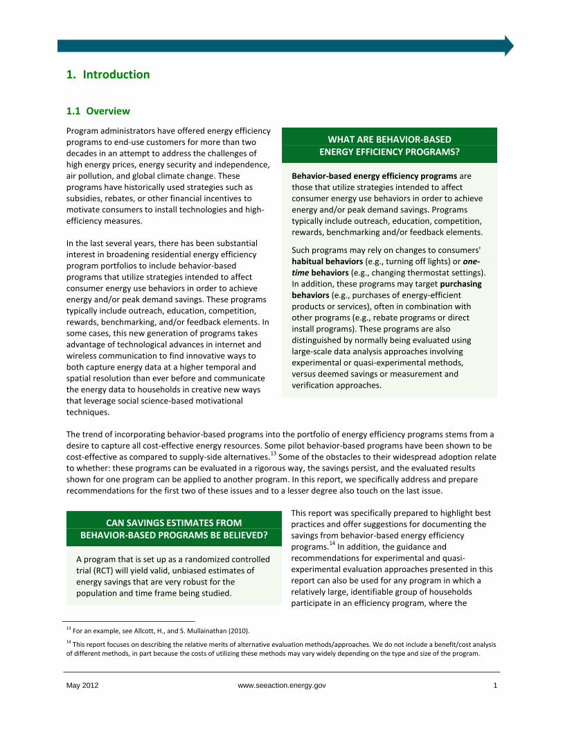
Program administrators have offered energy efficiency programs to end-use customers for more than two decades in an attempt to address the challenges of high energy prices, energy security and independence, air pollution, and global climate change. These programs have historically used strategies such as subsidies, rebates, or other financial incentives to motivate consumers to install technologies and high-efficiency measures.
In the last several years, there has been substantial interest in broadening residential energy efficiency program portfolios to include behavior-based programs that utilize strategies intended to affect consumer energy use behaviors in order to achieve energy and/or peak demand savings. These programs typically include outreach, education, competition, rewards, benchmarking, and/or feedback elements. In some cases, this new generation of programs takes advantage of technological advances in internet and wireless communication to find innovative ways to both capture energy data at a higher temporal and spatial resolution than ever before and communicate the energy data to households in creative new ways that leverage social science-based motivational techniques.
The trend of incorporating behavior-based programs into the portfolio of energy efficiency programs stems from a desire to capture all cost-effective energy resources. Some pilot behavior-based programs have been shown to be cost-effective as compared to supply-side alternatives.
13 Some of the obstacles to their widespread adoption relate
to whether: these programs can be evaluated in a rigorous way, the savings persist, and the evaluated results shown for one program can be applied to another program. In this report, we specifically address and prepare recommendations for the first two of these issues and to a lesser degree also touch on the last issue.
This report was specifically prepared to highlight best practices and offer suggestions for documenting the savings from behavior-based energy efficiency programs.
14 In addition, the guidance and
recommendations for experimental and quasi-experimental evaluation approaches presented in this report can also be used for any program in which a relatively large, identifiable group of households participate in an efficiency program, where the
13 For an example, see Allcott, H., and S. Mullainathan (2010).
14 This report focuses on describing the relative merits of alternative evaluation methods/approaches. We do not include a benefit/cost analysis of different methods, in part because the costs of utilizing these methods may vary widely depending on the type and size of the program.
WHAT ARE BEHAVIOR-BASED ENERGY EFFICIENCY PROGRAMS?
Behavior-based energy efficiency programs are those that utilize strategies intended to affect consumer energy use behaviors in order to achieve energy and/or peak demand savings. Programs typically include outreach, education, competition, rewards, benchmarking and/or feedback elements.
Such programs may rely on changes to consumers' habitual behaviors (e.g., turning off lights) or one-time behaviors (e.g., changing thermostat settings). In addition, these programs may target purchasing behaviors (e.g., purchases of energy-efficient products or services), often in combination with other programs (e.g., rebate programs or direct install programs). These programs are also distinguished by normally being evaluated using large-scale data analysis approaches involving experimental or quasi-experimental methods, versus deemed savings or measurement and verification approaches.
CAN SAVINGS ESTIMATES FROM BEHAVIOR-BASED PROGRAMS BE BELIEVED?
A program that is set up as a randomized controlled trial (RCT) will yield valid, unbiased estimates of energy savings that are very robust for the population and time frame being studied.

May 2012 www.seeaction.energy.gov 2
outcome of interest is energy savings quantified at a household level. Examples of such programs include mass-market information, education, and weatherization programs.
Because behavior-based programs do not specify, and generally cannot track, particular actions that result in energy savings, the impact evaluation of a behavior-based program is best done by measuring the actual energy use of program and non-program participants using a randomized controlled trial (RCT), and using this data to calculate an estimate of energy savings.
15
This method is at least as valid as other types of energy efficiency evaluation, measurement, and verification (EM&V) used to estimate first-year savings in other programs.
16 In cases for which RCTs are not
feasible, quasi-experimental approaches can also be used, although these are typically less reliable.
Other EM&V approaches, which involve site-specific measurement and verification (M&V) or deemed savings values and counting of specific measures or actions, are not applicable to behavior-based programs for at least three reasons. First, while evaluators of programs with pre-defined actions or measures such as rebate-type programs can count rebates as a proxy for the number of measure
installations, behavior-based programs typically have no such proxy (e.g., a program that gives out rewards for being the highest energy saver does not track the number of compact fluorescent light bulbs (CFLs) purchased by the winner or anyone else in the competition). Second, while survey questions for rebate, direct-install, or custom programs can be relatively straightforward (e.g., “Did you purchase and install an energy-efficient refrigerator in the last year?”), survey questions for some of the behaviors that are targeted by behavior-based programs may be more prone to exaggeration or error by the respondent (e.g., “How often do you typically turn off the lights after leaving a room compared to last year?”). Third, there are insufficient historical and applicable data on which to base stipulated (deemed) savings values for the wide range of behavior program designs and the wide range of populations they could serve. Conversely, programs that do not have identifiable participants (e.g., up-steam programs), have small populations of participants (e.g., custom measure industrial programs), or cannot easily define a control group (due to lack of data access, cost, or the impossibility of restricting program access) may find it less practical to take advantage of the accuracy and relatively low cost of RCT approaches.
1.2 Report Scope
In this report, we define behavior-based energy efficiency programs as those that utilize strategies intended to affect consumer energy use behaviors in order to achieve energy savings. Such programs may rely on changes to consumers' habitual behaviors (e.g., turning off lights) or one-time behaviors (e.g., changing thermostat settings). In addition, these programs may target purchasing behaviors (e.g., purchases of energy-efficient products or services), often in combination with other programs (e.g., rebate programs or direct-install programs). These programs are also distinguished by normally being evaluated using large-scale data analysis approaches involving
15 However, specific measure installations sometimes need to be tracked in order to assess double counting; see Section 3.2.
16 For example, many traditional programs are evaluated without the benefit of control groups, self-reported data, and/or use average or typical stipulated savings values and no actual energy measurements.
KEY DEFINITIONS
Treatment Group: the group of households that are assigned to receive the treatment
Control Group: the group of households that are assigned not to receive the program
Experimental Design: a method of controlling the way that a program is designed and evaluated in order to observe outcomes and infer whether or not the outcomes are caused by the program
Randomized Controlled Trial (RCT): a type of experimental design; a method of program evaluation in which households in a given population are randomly assigned into two groups—a treatment group and a control group—and the outcomes for these two groups are compared, resulting in unbiased program savings estimates
Quasi-Experimental Design: a method of program evaluation in which a treatment group and a control group are defined but households are not randomly assigned to these two groups, resulting in program savings estimates that may be biased

May 2012 www.seeaction.energy.gov 3
experimental or quasi-experimental methods, versus deemed savings or measurement and verification approaches. While some programs fit definitively in the behavior-based or non-behavior-based category, most programs contain behavior-based elements such as information and education. In this report, we focus only on programs whose savings can be determined using these experimental or quasi-experimental approaches, with large-scale data analysis.
Thus we exclude, for example, programs in which rebates are distributed to households (downstream rebate programs) or to manufacturers (upstream rebate programs) and installations with savings modeled on site-specific input assumptions; there are well-established best practices for these types of programs.
17
For the purposes of this report, we only consider behavior-based programs targeted at residential customers. In addition, we only consider impact evaluations for behavior-based programs where the outcome of interest is energy savings quantified at the household level. We do not consider other outcomes such as peak demand savings, market transformation, participation levels, spending levels, or number of rebates issued. We do not consider programs for which the energy savings are not quantified at the household level, such as college competitions that only have multi-unit level energy data. Because we are not considering peak demand savings, we also exclude time-based energy tariff programs.
18
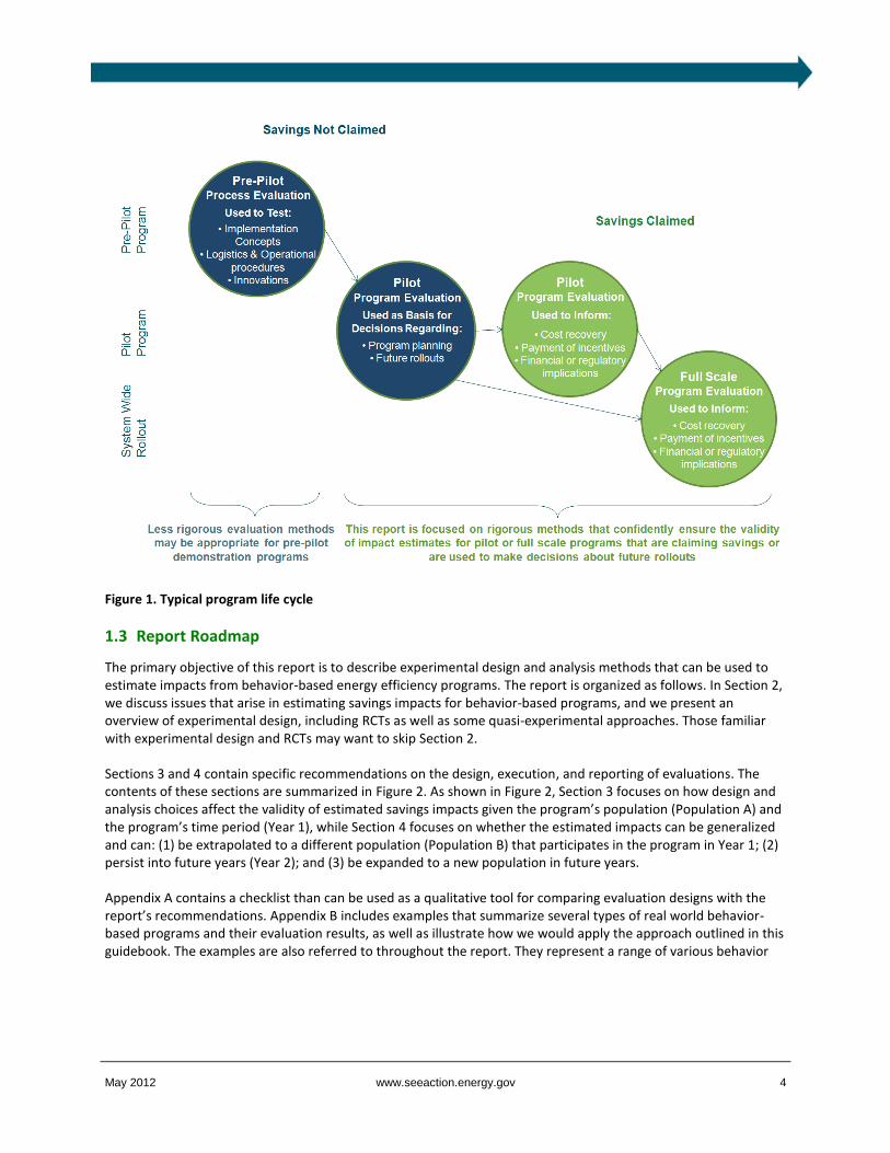
This guidebook is focused on providing recommendations of rigorous evaluation methods that confidently ensure the validity of impact estimates for pilot or full-scale behavior-based programs that are claiming savings or are being used as the basis for making decisions about future rollouts of large-scale or system-wide programs (see Figure 1). Other, less rigorous evaluation methods may be appropriate for small pre-pilot programs or demonstrations that are testing implementation concepts, logistic and operational procedures, or new, innovative approaches (e.g., a lower bar for statistical significance or an ethnographic survey approach).
19
In addition, there are several issues that are interesting but are outside of the scope of this report, including: how to decide what types of programs to adopt; how to determine which attributes of a program are most successful; how to determine which customer segments should be targeted; how to calculate the correct sample size; and an analysis of how much behavior-based programs and their evaluations cost.
20
17 For a few examples, see Energy Center of Wisconsin (2009), Regional Technical Forum (2011), Schiller (2007), Skumatz (2009), TecMarket Works (2004), The TecMarket Works Team (2006).
18 However, if for such a tariff program the outcome of interest is total annual energy savings, the recommendations and guidance in this report are applicable.
19 Ethnographic approaches collect qualitative data through methods such as interviews and direct observation.
20 Additional resources:
For a guide to implementing and evaluating programs, including guidelines for calculating the sample size (number of households needed in the study population to get a precise estimate, in Chapter 4) as well as other guidelines, see Duflo, Glennerster, and Kremer (2007).
For a technical guide to implementing and evaluating programs, see Imbens and Wooldridge (2009).
For a guide to implementing energy information feedback pilots that is applicable to non-feedback programs as well, see EPRI (2010).
For a book on how to evaluate and implement impact evaluation, see Gertler, Martinez, Premand, Rawlings, and Vermeersch (2010).
For an econometrics book, see Angrist and Pischke (2008).
For a document that discusses measurement and verification program design issues in behavior-based programs with a slightly different focus and target audience than this report, including a section on calculating sample size, see Sergici and Faruqui (2011).
For a discussion of using experiments to foster innovation and improve the effectiveness of energy efficiency programs, see: Sullivan (2009).
For a discussion of practical barriers and methods for overcoming barriers related to experimental design and RCTs, see Vine, Sullivan, Lutzenhiser, Blumstein, and Miller (2011).
For an overview of behavioral science and energy policy, see Allcott and Mullainathan (2010).
For non-behavior-based EM&V protocols and resources, see Schiller (2007) and Schiller (2011).
For an overview of residential energy feedback and behavior-based energy efficiency, see Haley and Mahone (2011).
May 2012 www.seeaction.energy.gov 4
Figure 1. Typical program life cycle
1.3 Report Roadmap
The primary objective of this report is to describe experimental design and analysis methods that can be used to estimate impacts from behavior-based energy efficiency programs. The report is organized as follows. In Section 2, we discuss issues that arise in estimating savings impacts for behavior-based programs, and we present an overview of experimental design, including RCTs as well as some quasi-experimental approaches. Those familiar with experimental design and RCTs may want to skip Section 2.
Sections 3 and 4 contain specific recommendations on the design, execution, and reporting of evaluations. The contents of these sections are summarized in Figure 2. As shown in Figure 2, Section 3 focuses on how design and analysis choices affect the validity of estimated savings impacts given the program’s population (Population A) and the program’s time period (Year 1), while Section 4 focuses on whether the estimated impacts can be generalized and can: (1) be extrapolated to a different population (Population B) that participates in the program in Year 1; (2) persist into future years (Year 2); and (3) be expanded to a new population in future years.
Appendix A contains a checklist than can be used as a qualitative tool for comparing evaluation designs with the report’s recommendations. Appendix B includes examples that summarize several types of real world behavior-based programs and their evaluation results, as well as illustrate how we would apply the approach outlined in this guidebook. The examples are also referred to throughout the report. They represent a range of various behavior

May 2012 www.seeaction.energy.gov 5
program types including feedback programs (e.g., home energy reports that provide households with specific energy use information and tips), in-home displays (IHDs) that stream constantly updated hourly energy use, online energy dashboards, and energy goal-setting challenges, as well as other types of information treatments such as non-personalized letters and energy saving tips sent in the mail or used as supplements to IHDs.
21
Appendix C contains specific examples of analysis models, with equations. In Appendix D, we discuss the savings impact analysis implications of two program design choices: enrollment method (opt-in or opt-out) and participant screening. While these choices do not affect the validity of the estimated program savings impacts, they do affect the interpretation of the estimates. We therefore discuss the various advantages and disadvantages of each method, but do not provide a recommended method.
1.4 How to Use This Report and Intended Audience
In this report, we generally rank different methods in terms of their value as a reliable means for estimating energy savings impacts on a scale of one to five stars.
22 The five-star methods are those that result in unbiased and precise
estimates of program impacts, while one-star methods result in estimates that are likely to be biased and/or imprecise. There may be various practical reasons why five-star methods are not feasible in certain situations. It may be that unbiased and precise estimates of program impacts cannot justify the costs associated with the more robust methods that generate such results. Thus, we have included other methods that have varying degrees of bias and precision so that program administrators, policymakers, and evaluators can make cost and accuracy tradeoffs that are applicable to their own resources and needs.
21 In this report, we provide four examples of real-world programs. The examples were chosen based on screening criteria that the programs comply with several of our evaluation recommendations. However, none of the examples provided represent an endorsement of the program.
22 Note that the rankings are made on the assumption that the evaluations are done correctly, use accurate data, have quality control mechanisms, and are completed by experienced people without prejudice in terms of the desired outcome of any analysis.
Figure 2. Relationships and influences between design and analysis choices, estimated savings, and different
populations and time periods
May 2012 www.seeaction.energy.gov 6
While the star rankings in each section are meant to represent the relative merits of each approach, sometimes there is an interactive effect in which the strength or weakness of a specific aspect of how the method is implemented affects the strength or weakness of that method. For example, collecting at least one year of pre-program energy usage data is always recommended, but if the evaluation design is not an experimental design, then collecting a year of historical data is truly crucial. We have captured these interactive effects in the discussion for each section, and also in the flow chart in Appendix A.
There are two intended audiences for the report. The Executive Summary (and Introduction and Checklist) is targeted to senior managers (at utilities, program administrators, regulatory agencies, and industry stakeholder groups) responsible for overseeing and reviewing efficiency program designs and their evaluations. This audience might also find that the second chapter on evaluation concepts and issues provides useful background for understanding the evaluation challenges associated with behavior-based programs. The main technical report, starting in Section 3, is targeted to staff responsible for reviewing efficiency program designs and their evaluations at utilities, practitioners who will be responsible for implementing residential behavior-based efficiency programs, and evaluation professionals responsible for the design and interpretation and use of the evaluation results.
May 2012 www.seeaction.energy.gov 7
2. Concepts and Issues in Estimation of Energy Savings
In this section, we first discuss the issues and uncertainty involved with estimating energy savings caused by a residential energy efficiency program, and the statistical methods for quantifying this uncertainty. We then present experimental design as a method for dealing with these issues in order to obtain savings estimates that are accurate and robust. Those familiar with causal inference, statistics, and experimental design may want to go directly to Section 3.
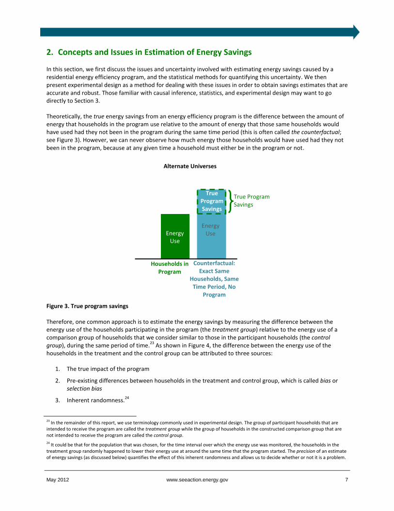
Theoretically, the true energy savings from an energy efficiency program is the difference between the amount of energy that households in the program use relative to the amount of energy that those same households would have used had they not been in the program during the same time period (this is often called the counterfactual; see Figure 3). However, we can never observe how much energy those households would have used had they not been in the program, because at any given time a household must either be in the program or not.
Therefore, one common approach is to estimate the energy savings by measuring the difference between the energy use of the households participating in the program (the treatment group) relative to the energy use of a comparison group of households that we consider similar to those in the participant households (the control group), during the same period of time.
23 As shown in Figure 4, the difference between the energy use of the
households in the treatment and the control group can be attributed to three sources:
1. The true impact of the program
2. Pre-existing differences between households in the treatment and control group, which is called bias or selection bias
3. Inherent randomness.24
23 In the remainder of this report, we use terminology commonly used in experimental design. The group of participant households that are intended to receive the program are called the treatment group while the group of households in the constructed comparison group that are not intended to receive the program are called the control group.
24 It could be that for the population that was chosen, for the time interval over which the energy use was monitored, the households in the treatment group randomly happened to lower their energy use at around the same time that the program started. The precision of an estimate of energy savings (as discussed below) quantifies the effect of this inherent randomness and allows us to decide whether or not it is a problem.
Households in Program
Counterfactual: Exact Same
Households, Same Time Period, No
Program
Energy Use
Energy Use
True Program Savings
Alternate Universes
True Program Savings
Figure 3. True program savings
May 2012 www.seeaction.energy.gov 8
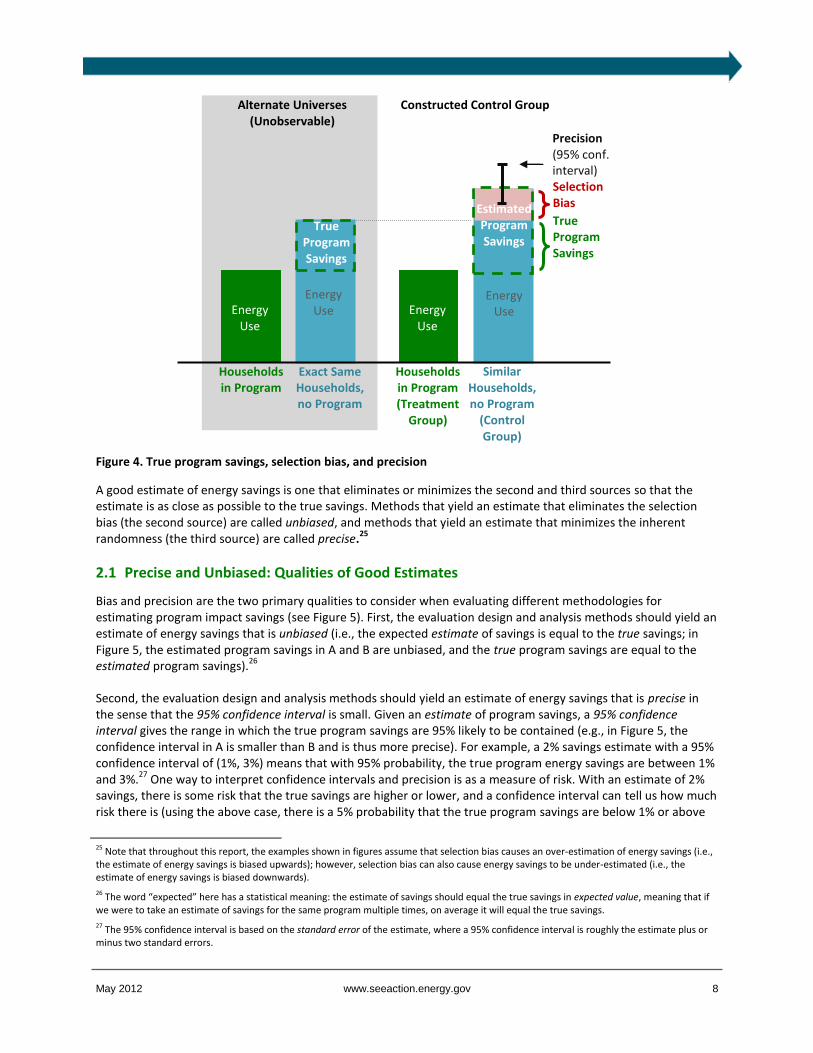
A good estimate of energy savings is one that eliminates or minimizes the second and third sources so that the estimate is as close as possible to the true savings. Methods that yield an estimate that eliminates the selection bias (the second source) are called unbiased, and methods that yield an estimate that minimizes the inherent randomness (the third source) are called precise.
25
2.1 Precise and Unbiased: Qualities of Good Estimates
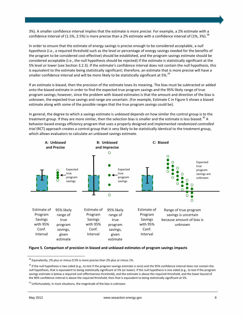
Bias and precision are the two primary qualities to consider when evaluating different methodologies for estimating program impact savings (see Figure 5). First, the evaluation design and analysis methods should yield an estimate of energy savings that is unbiased (i.e., the expected estimate of savings is equal to the true savings; in Figure 5, the estimated program savings in A and B are unbiased, and the true program savings are equal to the estimated program savings).
26
Second, the evaluation design and analysis methods should yield an estimate of energy savings that is precise in the sense that the 95% confidence interval is small. Given an estimate of program savings, a 95% confidence interval gives the range in which the true program savings are 95% likely to be contained (e.g., in Figure 5, the confidence interval in A is smaller than B and is thus more precise). For example, a 2% savings estimate with a 95% confidence interval of (1%, 3%) means that with 95% probability, the true program energy savings are between 1% and 3%.
27 One way to interpret confidence intervals and precision is as a measure of risk. With an estimate of 2%
savings, there is some risk that the true savings are higher or lower, and a confidence interval can tell us how much risk there is (using the above case, there is a 5% probability that the true program savings are below 1% or above
25 Note that throughout this report, the examples shown in figures assume that selection bias causes an over-estimation of energy savings (i.e., the estimate of energy savings is biased upwards); however, selection bias can also cause energy savings to be under-estimated (i.e., the estimate of energy savings is biased downwards).
26 The word “expected” here has a statistical meaning: the estimate of savings should equal the true savings in expected value, meaning that if we were to take an estimate of savings for the same program multiple times, on average it will equal the true savings.
27 The 95% confidence interval is based on the standard error of the estimate, where a 95% confidence interval is roughly the estimate plus or minus two standard errors.
Figure 4. True program savings, selection bias, and precision
Households in Program
Exact Same Households, no Program
Energy Use
Energy Use
Similar Households, no Program
(Control Group)
Energy Use
Estimated Program Savings
Selection Bias
True Program Savings
Households in Program (Treatment
Group)
Energy Use
Alternate Universes (Unobservable)
Constructed Control Group
Precision (95% conf. interval)
True Program Savings
May 2012 www.seeaction.energy.gov 9
3%). A smaller confidence interval implies that the estimate is more precise. For example, a 2% estimate with a confidence interval of (1.5%, 2.5%) is more precise than a 2% estimate with a confidence interval of (1%, 3%).
28
In order to ensure that the estimate of energy savings is precise enough to be considered acceptable, a null hypothesis (i.e., a required threshold such as the level or percentage of energy savings needed for the benefits of the program to be considered cost-effective) should be established, and the program savings estimate should be considered acceptable (i.e., the null hypothesis should be rejected) if the estimate is statistically significant at the 5% level or lower (see Section 3.2.3). If the estimate’s confidence interval does not contain the null hypothesis, this is equivalent to the estimate being statistically significant; therefore, an estimate that is more precise will have a smaller confidence interval and will be more likely to be statistically significant at 5%.
29
If an estimate is biased, then the precision of the estimate loses its meaning. The bias must be subtracted or added onto the biased estimate in order to find the expected true program savings and the 95% likely range of true program savings; however, since the problem with biased estimates is that the amount and direction of the bias is unknown, the expected true savings and range are uncertain. (For example, Estimate C in Figure 5 shows a biased estimate along with some of the possible ranges that the true program savings could be).
In general, the degree to which a savings estimate is unbiased depends on how similar the control group is to the treatment group. If they are more similar, then the selection bias is smaller and the estimate is less biased.
30 A
behavior-based energy efficiency program that uses a properly designed and implemented randomized controlled trial (RCT) approach creates a control group that is very likely to be statistically identical to the treatment group, which allows evaluators to calculate an unbiased savings estimate.
28 Equivalently, 2% plus or minus 0.5% is more precise than 2% plus or minus 1%.
29 If the null hypothesis is two sided (e.g., to test if the program savings estimate is zero) and the 95% confidence interval does not contain the null hypothesis, that is equivalent to being statistically significant at 5% (or lower). If the null hypothesis is one sided (e.g., to test if the program savings estimate is below a required cost-effectiveness threshold), and the estimate is above the required threshold, and the lower bound of the 90% confidence interval is above the required threshold, then that is equivalent to being statistically significant at 5%.
30 Unfortunately, in most situations, the magnitude of the bias is unknown.
Estimate of Program Savings
with 95% Conf.
Interval
A: Unbiased and Precise
Expected true program savings
95% likely range of
true program savings,
given estimate
Estimate of Program Savings
with 95% Conf.
Interval
B: Unbiased and Imprecise
Expected true program savings
95% likely range of
true program savings,
given estimate
Estimate of Program Savings
with 95% Conf.
Interval
C: Biased
Expected true program savings are unknown
Range of true program savings is uncertain
because amount of bias is unknown
Figure 5. Comparison of precision in biased and unbiased estimates of program savings impacts

May 2012 www.seeaction.energy.gov 10
The precision of the savings estimate depends on how much information (i.e., how much data and how many variables that are informative to estimating an effect) is used by the analysis model and how much variation there is in the data being measured. One way to increase precision is to increase the number of households in both the treatment and control group; other approaches include covering a longer time period of energy use data, using more granular energy data, including extra information about weather, or adding other informative variables.
2.2 Randomized Controlled Trials
If a program’s evaluation method is set up as an RCT in which the population of interest (e.g., single family homes in Denver) is randomly assigned to either a treatment or control group, then the selection bias is eliminated, leading to an estimate of program energy savings that is unbiased.
31 This is the only method that eliminates
selection bias (e.g., see Figure 6: an RCT control group yields an unbiased estimate of program savings whereas a non-RCT control group yields a biased estimate).
32 Therefore, using an RCT is a key initial step in ensuring the
validity of estimates of program savings for behavior-based efficiency programs.33
While RCTs may involve a higher initial setup cost than other evaluation approaches, they are an attractive risk management strategy because the program impact estimates are more accurate. The precision of the estimate is determined by the number of households, the analysis method, and the number of informative variables included in the analysis.
31 See, for example, Angrist and Pischke (2008); Duflo (2004); Imbens and Wooldridge (2009); LaLonde (1986).
32 For example, if a matched control group method is used, one could always make the assumption that all relevant characteristics are being matched, and that any other characteristics not included in the matching, as well as any unobservable characteristics, have no impact on the outcome. However, this is a very strong assumption, which is not amenable to testing.
33 Randomized Controlled Trials are the gold standard of program evaluation used in many other areas. For example, the U.S. Food and Drug Administration (FDA) uses RCTs to assess whether medications are safe for public consumption.
Households in Program
Exact Same Households, no Program
Energy Use
Energy Use
True Program Savings
Similar Households, no Program
(Control Group)
Energy Use
Estimated Program Savings
Selection Bias
True Program Savings
Households in Program (Treatment
Group)
Energy Use
Unbiased: Selection Bias Eliminated
Energy Use
Similar Households, no Program
(Control Group)
Estimated Program Savings
Households in Program (Treatment
Group)
Energy Use
True Program Savings
Alternate Universes (Unobservable)
RCT Control Group Non-RCT Control Group
Figure 6. An RCT control group compared to a non-RCT control group
May 2012 www.seeaction.energy.gov 11
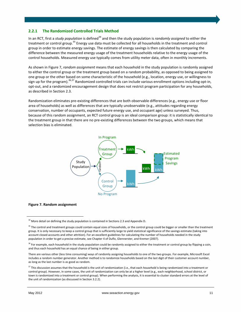
2.2.1 The Randomized Controlled Trials Method
In an RCT, first a study population is defined34
and then the study population is randomly assigned to either the treatment or control group.
35 Energy use data must be collected for all households in the treatment and control
group in order to estimate energy savings. The estimate of energy savings is then calculated by comparing the difference between the measured energy usage of the treatment households relative to the energy usage of the control households. Measured energy use typically comes from utility meter data, often in monthly increments.
As shown in Figure 7, random assignment means that each household in the study population is randomly assigned to either the control group or the treatment group based on a random probability, as opposed to being assigned to one group or the other based on some characteristic of the household (e.g., location, energy use, or willingness to sign up for the program).
36,37 Randomized controlled trials can include various enrollment options including opt-in,
opt-out, and a randomized encouragement design that does not restrict program participation for any households, as described in Section 2.3.
Randomization eliminates pre-existing differences that are both observable differences (e.g., energy use or floor area of households) as well as differences that are typically unobservable (e.g., attitudes regarding energy conservation, number of occupants, expected future energy use, and occupant age) unless surveyed. Thus, because of this random assignment, an RCT control group is an ideal comparison group: it is statistically identical to the treatment group in that there are no pre-existing differences between the two groups, which means that selection bias is eliminated.
34 More detail on defining the study population is contained in Sections 2.3 and Appendix D. 35 The control and treatment groups could contain equal sizes of households, or the control group could be bigger or smaller than the treatment group. It is only necessary to keep a control group that is sufficiently large to yield statistical significance of the savings estimate (taking into account closed accounts and other attrition). For an excellent guidelines for calculating the number of households needed in the study population in order to get a precise estimate, see Chapter 4 of Duflo, Glennerster, and Kremer (2007).
36 For example, each household in the study population could be randomly assigned to either the treatment or control group by flipping a coin, and thus each household has an equal chance of being in either group.
There are various other (less time consuming) ways of randomly assigning households to one of the two groups. For example, Microsoft Excel includes a random number generator. Another method is to randomize households based on the last digit of their customer account number, as long as the last number is as good as random.
37 This discussion assumes that the household is the unit of randomization (i.e., that each household is being randomized into a treatment or control group). However, in some cases, the unit of randomization can only be at a higher level (e.g., each neighborhood, school district, or town is randomized into a treatment or control group). When performing the analysis, it is essential to cluster standard errors at the level of the unit of randomization (as discussed in Section 3.2.2).
Estimated Program Savings Study
Population
In Program
Treatment Group
Control Group
No Program
kWh
kWh
kWh kWh
Figure 7. Random assignment
ran
do
m

May 2012 www.seeaction.energy.gov 12
2.2.2 Free Riders, Spillover, and Rebound Effects
It is worth pointing out one specific type of selection bias that RCTs eliminate. Often when program impacts are estimated, one difficulty that arises is whether the households in the program would have saved energy even in the absence of the program (e.g., a household was already planning to install R-30 attic insulation at the same time that they received information about an efficiency program that was offering a rebate for installing R-30 attic insulation). These households are typically called free riders by efficiency evaluators.
As shown in Figure 8, RCTs eliminate this free-rider concern during the study period because the treatment and control groups each contain the same number of free riders through the process of random assignment to the treatment or control groups. When the two groups are compared, the energy savings from the free riders in the control group cancel out the energy savings from the free riders in the treatment group, and the resulting estimate of program energy savings is an unbiased estimate of the savings caused by the program (the true program savings). This is one of the main benefits of an RCT over traditional evaluation methods.
38
Participant spillover, in which participants engage in additional energy efficiency actions outside of the program as a result of the program, is also automatically captured by an RCT design for energy use that is measured within a household.
39 In addition to participant spillover, non-participant spillover issues in which a program influences the
energy use of non-program participants are not addressed by RCTs. For example, a program may indirectly influence households in the control group, or may influence the market provision of energy-efficient equipment to everyone inside and outside of the control group, whether they are a participant or non-participant in the specific program being evaluated. In these cases in which non-participant spillover exists, an evaluation that relies on RCT design could underestimate the total program-influenced savings.
40
38 An RCT design produces an estimate of net energy savings, and thus also addresses rebound effects or take-back during the study period, which can occur if consumers increase energy use as a result of a new device’s improved efficiency. However, rebound effects after the study period are not accounted for.
39 However, additional spillover effects such as workplace behavior or gas-related efficiency behaviors if only electricity is measured are not included.
40 It is possible to explicitly experiment with this in order to determine the spillover effects. For example, an experiment could be conducted in which the impacts of the intervention are observed for both the households in the experiment as well as others, and the impacts in two or more communities are compared. This type of experiment is often used in medicine and epidemiology.
Energy Use
RCT Control Group,
no Program
Estimated Program Savings
Households in Program
Energy Use
True Program Savings
RCT Control Group
Figure 8. Randomized controlled trials solve the free-rider problem
Free Riders Free Riders

May 2012 www.seeaction.energy.gov 13
2.3 Randomized Controlled Trials with Various Enrollment Options
There are three basic program enrollment options: opt-out enrollment, opt-in enrollment, and encouragement design, which does not restrict or withhold participation in the program to any household.
41 Program designs with
any of these enrollment options can utilize RCTs for evaluation and thus each enrollment option can yield unbiased savings estimates. With any of the enrollment options, the random assignment of households into treatment and control groups is the crucial step. All data from the randomization point forward should be analyzed to ensure internal validity.
42
When implementing RCTs with any of these three enrollment options, the first step is defining the target market and the eligible households that are included in the study population (i.e., the screening criteria).
43 Often this
screening process restricts the study population to specific geographies (zip codes or service areas), specific demographics (low income, medical needs, elderly), specific customer characteristics (high energy users, dual fuel use, length of customer bill history), and specific data requirements (one year of historical energy data available, census information is available, smart meter installed). Another way to reduce the size of the study population (if there are budgetary or other restrictions on program size) is to randomly select households out of a larger population in order to form a smaller subset of households.
44 This method has the advantage that results from the
smaller subset of households is more likely to be externally valid, to the degree that the results can be extrapolated to the larger population for the same time period as the analysis (see Section 4.1). Appendix D has a more in-depth discussion of enrollment options.
2.3.1 Randomized Controlled Trials with Opt-Out Enrollment
In some cases, program administrators may want to enroll households using an opt-out method.45
As shown in Figure 9, in an RCT with an opt-out recruitment strategy, after households have been evaluated for program eligibility (i.e., screened in or screened out), the remaining households are placed in the study population and are randomly assigned to either the control group or the treatment group. The treatment group receives the program (but are allowed to opt out), and the control group does not receive the program (and are not allowed to opt in).
46,47 Energy use data must be collected for all of the households in the control and treatment group, whether or
not they opt out, in order to estimate energy savings without bias. If the households that opt out are excluded from the treatment group, as discussed in Section 3.2.4, then the results will suffer from selection bias: the households in the control group are no longer the same types of households as those in the treatment group.
41 We have represented the three options that are the most commonly used in energy programs, and have mentioned some others in footnotes. In addition, there are randomization designs that are more complex than those described in this section; factorial designs, for example.
42 Essentially, randomization can happen before or after the enrollment decision (opt-in or opt-out); however, data must be analyzed for all households in the randomized control and treatment groups. So if randomization occurs before opt-in or opt-out enrollment, then data from all households must be analyzed, even if those households later decide to opt out or opt in. If randomization occurs after opt-in or opt-out enrollment, then only data from the households that enrolled (and were subsequently randomized) have to be analyzed. The three most commonly used methods are (1) randomization followed by opt-out (Section 2.3.1), (2) opt-in followed by randomization (Section 2.3.2), and (3) randomization followed by opt-in, or RED (Section 2.3.3).
43 The eligible households (i.e., those that are screened in) comprise the study population, which are the households that will be approached and marketed to participate and enroll in the program.
44 One way to randomly select households out of a larger population is to perform stratified sampling, in which household types are broken up into subsets (e.g., high, medium, and low energy users), and then certain proportions of households are randomly selected from each of these subsets. If some of the subsets are over or under sampled (as is commonly done in the load research community), then the data may need to be weighted in order to correct for this in the analysis.
45 See Appendix D for a discussion of enrollment methods.
46 Alternately, households in the study population can first be informed that they are going to be part of the study but are allowed to opt out. After households have opted out or not, the households that have not opted out are randomly assigned to either a control group or a treatment group. This variation is equivalent to Figure 10 where “Opt In” in the figure is replaced with “Don’t Opt Out,” and “Don’t Opt In” in the figure is replaced with “Opt Out”.
47 If the households in the control group are allowed to opt in, then this would be a randomized encouragement design (Section 2.3.3).
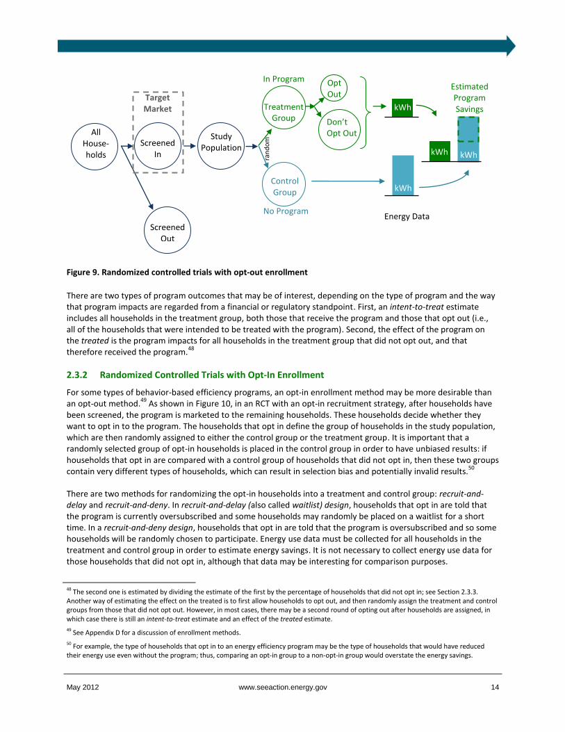
May 2012 www.seeaction.energy.gov 14
There are two types of program outcomes that may be of interest, depending on the type of program and the way that program impacts are regarded from a financial or regulatory standpoint. First, an intent-to-treat estimate includes all households in the treatment group, both those that receive the program and those that opt out (i.e., all of the households that were intended to be treated with the program). Second, the effect of the program on the treated is the program impacts for all households in the treatment group that did not opt out, and that therefore received the program.
48
2.3.2 Randomized Controlled Trials with Opt-In Enrollment
For some types of behavior-based efficiency programs, an opt-in enrollment method may be more desirable than an opt-out method.
49 As shown in Figure 10, in an RCT with an opt-in recruitment strategy, after households have
been screened, the program is marketed to the remaining households. These households decide whether they want to opt in to the program. The households that opt in define the group of households in the study population, which are then randomly assigned to either the control group or the treatment group. It is important that a randomly selected group of opt-in households is placed in the control group in order to have unbiased results: if households that opt in are compared with a control group of households that did not opt in, then these two groups contain very different types of households, which can result in selection bias and potentially invalid results.
50
There are two methods for randomizing the opt-in households into a treatment and control group: recruit-and-delay and recruit-and-deny. In recruit-and-delay (also called waitlist) design, households that opt in are told that the program is currently oversubscribed and some households may randomly be placed on a waitlist for a short time. In a recruit-and-deny design, households that opt in are told that the program is oversubscribed and so some households will be randomly chosen to participate. Energy use data must be collected for all households in the treatment and control group in order to estimate energy savings. It is not necessary to collect energy use data for those households that did not opt in, although that data may be interesting for comparison purposes.
48 The second one is estimated by dividing the estimate of the first by the percentage of households that did not opt in; see Section 2.3.3. Another way of estimating the effect on the treated is to first allow households to opt out, and then randomly assign the treatment and control groups from those that did not opt out. However, in most cases, there may be a second round of opting out after households are assigned, in which case there is still an intent-to-treat estimate and an effect of the treated estimate.
49 See Appendix D for a discussion of enrollment methods.
50 For example, the type of households that opt in to an energy efficiency program may be the type of households that would have reduced their energy use even without the program; thus, comparing an opt-in group to a non-opt-in group would overstate the energy savings.
Estimated Program Savings
Screened In
Study Population
OptOut
Control Group
No Program
kWh
kWh
kWh kWh
Don’t Opt Out
All
House-holds
Screened Out
Figure 9. Randomized controlled trials with opt-out enrollment
In Program
Treatment Group
Energy Data
Target Market
ran
do
m
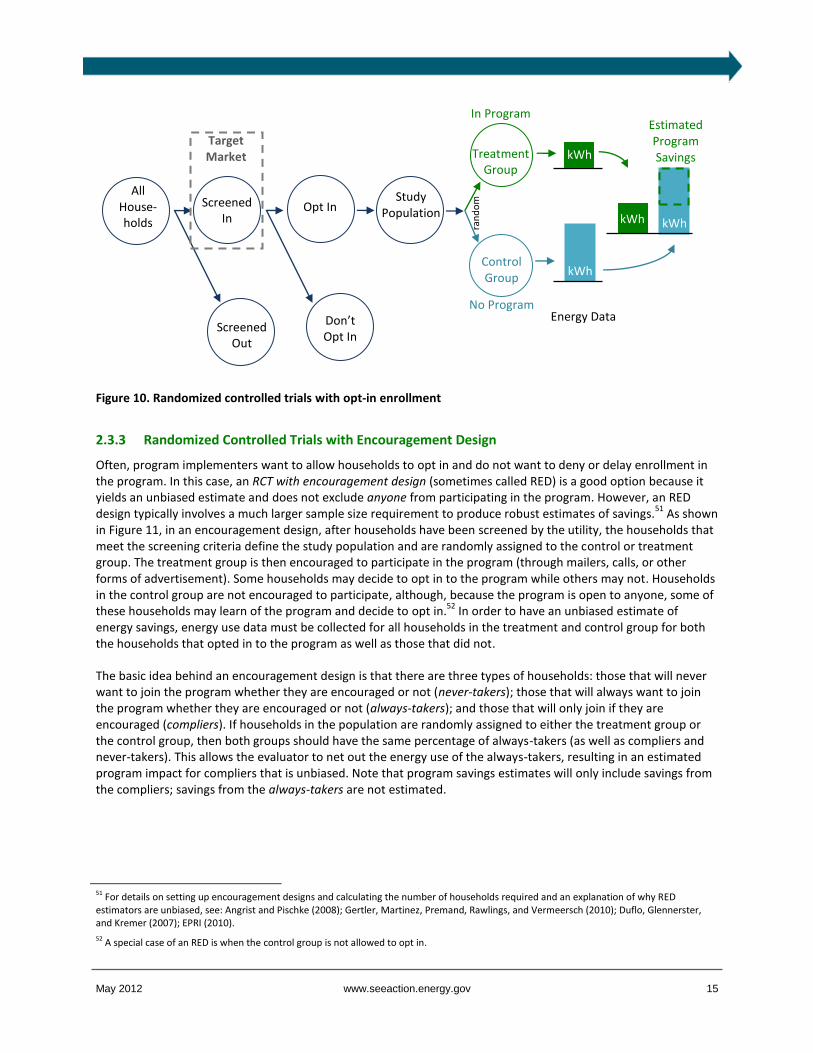
May 2012 www.seeaction.energy.gov 15
2.3.3 Randomized Controlled Trials with Encouragement Design
Often, program implementers want to allow households to opt in and do not want to deny or delay enrollment in the program. In this case, an RCT with encouragement design (sometimes called RED) is a good option because it yields an unbiased estimate and does not exclude anyone from participating in the program. However, an RED design typically involves a much larger sample size requirement to produce robust estimates of savings.
51 As shown
in Figure 11, in an encouragement design, after households have been screened by the utility, the households that meet the screening criteria define the study population and are randomly assigned to the control or treatment group. The treatment group is then encouraged to participate in the program (through mailers, calls, or other forms of advertisement). Some households may decide to opt in to the program while others may not. Households in the control group are not encouraged to participate, although, because the program is open to anyone, some of these households may learn of the program and decide to opt in.
52 In order to have an unbiased estimate of
energy savings, energy use data must be collected for all households in the treatment and control group for both the households that opted in to the program as well as those that did not.
The basic idea behind an encouragement design is that there are three types of households: those that will never want to join the program whether they are encouraged or not (never-takers); those that will always want to join the program whether they are encouraged or not (always-takers); and those that will only join if they are encouraged (compliers). If households in the population are randomly assigned to either the treatment group or the control group, then both groups should have the same percentage of always-takers (as well as compliers and never-takers). This allows the evaluator to net out the energy use of the always-takers, resulting in an estimated program impact for compliers that is unbiased. Note that program savings estimates will only include savings from the compliers; savings from the always-takers are not estimated.
51 For details on setting up encouragement designs and calculating the number of households required and an explanation of why RED estimators are unbiased, see: Angrist and Pischke (2008); Gertler, Martinez, Premand, Rawlings, and Vermeersch (2010); Duflo, Glennerster, and Kremer (2007); EPRI (2010).
52 A special case of an RED is when the control group is not allowed to opt in.
Estimated Program Savings
Screened In
Study Population Opt In
In Program
Treatment Group
Control Group
No Program
kWh
kWh
kWh kWh
Don’t Opt In
All
House-holds
Figure 10. Randomized controlled trials with opt-in enrollment
Screened Out
Energy Data
Target Market
ran
do
m
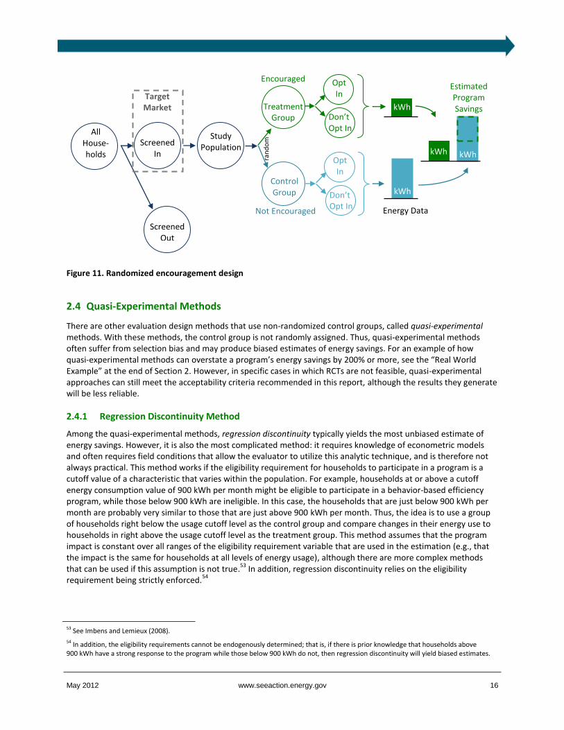
May 2012 www.seeaction.energy.gov 16
2.4 Quasi-Experimental Methods
There are other evaluation design methods that use non-randomized control groups, called quasi-experimental methods. With these methods, the control group is not randomly assigned. Thus, quasi-experimental methods often suffer from selection bias and may produce biased estimates of energy savings. For an example of how quasi-experimental methods can overstate a program’s energy savings by 200% or more, see the “Real World Example” at the end of Section 2. However, in specific cases in which RCTs are not feasible, quasi-experimental approaches can still meet the acceptability criteria recommended in this report, although the results they generate will be less reliable.
2.4.1 Regression Discontinuity Method
Among the quasi-experimental methods, regression discontinuity typically yields the most unbiased estimate of energy savings. However, it is also the most complicated method: it requires knowledge of econometric models and often requires field conditions that allow the evaluator to utilize this analytic technique, and is therefore not always practical. This method works if the eligibility requirement for households to participate in a program is a cutoff value of a characteristic that varies within the population. For example, households at or above a cutoff energy consumption value of 900 kWh per month might be eligible to participate in a behavior-based efficiency program, while those below 900 kWh are ineligible. In this case, the households that are just below 900 kWh per month are probably very similar to those that are just above 900 kWh per month. Thus, the idea is to use a group of households right below the usage cutoff level as the control group and compare changes in their energy use to households in right above the usage cutoff level as the treatment group. This method assumes that the program impact is constant over all ranges of the eligibility requirement variable that are used in the estimation (e.g., that the impact is the same for households at all levels of energy usage), although there are more complex methods that can be used if this assumption is not true.
53 In addition, regression discontinuity relies on the eligibility
requirement being strictly enforced.54
53 See Imbens and Lemieux (2008).
54 In addition, the eligibility requirements cannot be endogenously determined; that is, if there is prior knowledge that households above 900 kWh have a strong response to the program while those below 900 kWh do not, then regression discontinuity will yield biased estimates.
Estimated Program Savings
Screened In
Study Population
Opt In
Control Group
Not Encouraged
kWh
kWh
kWh kWh
Don’t Opt In
All
House-holds
Screened Out
Figure 11. Randomized encouragement design
Encouraged
Treatment Group
Opt In
Don’t Opt In Energy Data
Target Market
ran
do
m

May 2012 www.seeaction.energy.gov 17
2.4.2 Matched Control Group Method
If it is not possible to create a randomized control group, then savings estimates could be calculated by constructing a non-random control group made up of households that are as similar to the treatment group as possible. The challenge with a matched control group method is that households have both observable characteristics (e.g., level of energy use, zip code, presence of central air conditioning) that could potentially be matched, and unobservable characteristics (e.g., energy attitudes, or propensity to opt in to an energy efficiency program) that are harder or impossible to match.
Match on Observables A matched control group or post-matched control group is a non-random control group where the observable characteristics of the households in the program are known or measured, and then a control group that best matches those characteristics is constructed. The idea is to create a control group that is as similar as possible to the treatment group. For example, with an opt-in program, it may be true that all households that opted in lived in a rural area and had high energy use. In this case, a matched control group might include households in the same rural area with high energy use that did not opt in to the program. This control group is matched on two observable characteristics (energy use and location). However, it is not matched on the unobserved variable of propensity to opt in: it ignores the fact that households that opt in to a program are fundamentally different than those that do not opt in. For example, these households may be more inclined to conserve energy than those that are not interested in participating in the program. In the case of an opt-out program, the households that could be used in the matched control group are either those that were screened out or those that opted out.
Propensity Score Matching Propensity score matching attempts to match households on both observable and unobservable characteristics for the case of an opt-in program. This method uses observable characteristics to predict the probability that a household will decide to opt in to a program, and then chooses households that had a high probability of opting in to the program but did not actually opt in to be in the control group.
While this method is better than a matching method without propensity scores, it still assumes that whatever observable characteristics of the households were used to calculate the propensity score are sufficient to explain any unobservable differences between the treatment and non-random control group. This method is more credible if accurate detailed household demographic information is obtainable, rather than generic categories (e.g., broad census demographics or categories such as “urban youth”). However, in cases for which RCTs and regression discontinuity methods are impractical, propensity score matching is an acceptable method.
2.4.3 Variation in Adoption (With a Test of Assumptions)
This variation in adoption approach takes advantage of variation in the timing of program adoption. This allows for the comparison of the energy usage of households that opt in to the energy usage of households that have not yet opted in but will ultimately opt in at a later point. It relies on the assumption that in any given month, households that have already opted in and households that will opt in soon are the same types of households. For this assumption to be valid, households must decide to opt in to the program at different times, and the decision of each household to opt in during any particular month should be essentially random, and only influenced by marketing exposure and awareness of the program (this is different than an RCT with a recruit-and-delay design, in which households do not decide when to opt in but rather are randomly assigned different times to opt in). The decision to opt in should not be related to observable or unobservable household characteristics (e.g., energy conservation attitudes). Because the validity of the estimated program impact depends upon this assumption, it should be tested to the extent possible with a test of assumptions.
55
55One way to test it is by conducting a duration analysis, which tests whether household adoption in any particular month is driven by marketing activity, as opposed to observed household characteristics or unobserved heterogeneity. Another test is to determine if the energy usage of households before they opt in differs between households that opt in during one particular month as opposed to another month. In

May 2012 www.seeaction.energy.gov 18
In addition, if the energy savings due to the program do not persist over time, then the estimated program impact will be biased and thus require corrections.
56 If the assumption that the timing of household program adoption is
essentially random is valid, then this method is as good as a regression discontinuity method. However, although the assumption can be tested and found to not hold, it cannot be found to hold with certainty (e.g., household adoption may correspond to unobservable characteristics, such as willingness to opt in during a specific season).
2.4.4 Pre-Post Energy Use Method
Another quasi-experimental method is to compare the energy use of households in the treatment group after they were enrolled in the program to the same households’ historical energy use prior to program enrollment. In effect, this means that each household in the treatment group is its own non-random control group. This is called a pre-post; within subjects; or interrupted time series design analysis.
The challenge in using this method is that there are many other factors (independent variables) that may influence energy use before, during, and after the program that are not captured with this method. Some of these factors, such as differences in weather or number of occupants, may be reliably accounted for in the analysis. However, other factors are less easily observed and/or accounted for. For example, the economy could have worsened, leading households to decrease energy (even if there were no program), or a pop culture icon such as Katy Perry could suddenly decide to advocate for energy efficiency. With a pre-post analysis, there is no way to discern and separate the impact of other influences (e.g., economic recession) that may affect energy use over time compared to the impact of the behavior-based efficiency program leading to an estimate of energy savings that could be biased.
57
addition, propensity score matching can be used to further verify the assumption by accounting for potentially varying demographics of the households over time as they opt in to the program.
56 For a detailed description of a robust variation in adoption methodology, see Harding and Hsiaw (2011).
57 However, in programs outside the scope of this report such as critical peak pricing or critical peak rebates, a pre-post method may be less biased. This method should only be considered when the experimental factor can be presented repeatedly so that the difference between the behavior when it is present and when it is not present is observable. It is not really appropriate for circumstances where the effect of the experimental factor is expected to persist for a long period of time after exposure or is continuously presented throughout the experiment (e.g., time of use or information feedback).

May 2012 www.seeaction.energy.gov 19
REAL WORLD EXAMPLEa
Energy Savings Estimates from RCT versus Quasi-Experimental Approaches
Most Opowerb programs use an RCT design, where households are recruited using an opt-out method. In an
evaluation of 17 different Opower programs, Allcott (2011) calculated program savings in three ways: (1) using the RCT and comparing the treatment to the control group to estimate savings, which most likely leads to an unbiased savings estimate (labeled “RCT” in the graph); (2) ignoring the RCT and instead using a quasi-experimental approach comparing each household in the treatment group to their energy use before the program (labeled “Pre-Post” in the graph); and (3) ignoring the experimental design and instead using a quasi-experimental approach comparing the change in energy use of households in the treatment group to the change in energy use of households in a constructed comparison group of nearby households with similar energy usage (labeled “Matched” in the graph).
As is evident in the graph, the two quasi-experimental estimates of energy savings typically produce larger estimates of savings that are outside the error bounds of the RCT estimates, suggesting that they are biased. Possible explanations include that the pre-post method does not control for changes in the economy (i.e., households would have reduced energy use even in the absence of the program because of higher unemployment rates), and that the matched method includes households in the control group that may have different characteristics than those in the treatment group (e.g., they may have a different set of utility programs marketed to them).
H. Allcott, “Social Norms and Energy Conservation,” Journal of Public Economics (2011)
a In this report, we provide examples of actual programs’ evaluations. The examples were chosen based on a screening criterion
that the programs comply with several of our evaluation recommendations and were implemented by different entities and/or in different parts of the country. None of the examples provided in this report represent a specific endorsement of a program design, program implementer, or evaluator.
b Opower is a company contracted by energy efficiency program administrators to provide households with personalized
information about their energy use via paper or an online portal.
RCT 95% Conf Int Pre-Post Matched
Ener
gy U
se

May 2012 www.seeaction.energy.gov 20
3. Internal Validity: Validity of Estimated Savings Impacts for Initial Program
In this section, we focus on how different design and analysis choices affect the validity of estimated savings impacts for the subject population and the initial time period (i.e., the first year[s] of a behavior-based energy efficiency program). This section focuses on issues relating to the internal validity of savings estimates, seeking to answer the question: “For the given population during the initial time period, was the estimated impact caused by the program (as opposed to other factors)?” Methods and best practices for ensuring internal validity are well established, and are currently being used for a number of behavior-based programs in order to claim savings. The contents of this section and Section 4 are summarized in Figure 2.
We refer to the subject (or evaluated) population and time period in this and future sections as the initial population and time period. We assume that program implementers will often be interested in expanding the program over time and to other populations; thus, we examine whether the estimated savings for this initial program can be generalized and applied to new populations in Section 4.1 and to future years in Section 4.2 (commonly referred to as external validity).
3.1 Design Choices
3.1.1 Issue A: Evaluation Design
The choice of evaluation design is the most important factor in creating estimates of program impacts that are unbiased and internally valid. In this report, we define evaluation design as the way in which a control group is constructed and compared to the treatment group in order to estimate the program savings impacts.
58 An experimental design with a randomized
controlled trial (RCT) is the preferred evaluation design method because it yields estimates of program savings impacts that are unbiased (see Section 2.2). On the other hand, quasi-experimental methods, which have non-randomized control groups, have varying degrees of bias (see Section 2.4). These methods are ranked according to their level of bias in Table 1: more stars indicate less bias; fewer stars indicate that the method yields estimates of program savings impacts that are likely to be more biased.
59
58 This is also called the identification strategy or the method of causal inference.
59 Note that these rankings assume that the evaluation design was performed correctly; for example, if the evaluation design is an RCT, then randomization should be done as specified in Section 2.3.
REAL WORLD EXAMPLE
Evaluation Design: Puget Sound Energy’s Home Energy Reports Program
Method: RCT (Opt-out)
In 2008, Puget Sound Energy (PSE) implemented one of the nation’s first Home Energy Report (HER) programs designed to encourage energy conservation behavior at the household level through normative messaging. Administered by Opower, the PSE program provided HERs to nearly 40,000 households. The reports compared the subject household’s energy usage with that of neighboring homes, applying peer pressure to influence behavior and garner energy savings.
The PSE program used an RCT with opt-out recruitment. From all the households in PSE territory, the program administrator selected a group of 83,800 households that met certain criteria (e.g., single family, adequate utility bill data). The program then randomly assigned 37,775 of those households to the treatment group that received HERs on a monthly or quarterly basis. The remaining 44,025 households were assigned to the control group and received no HER.
KEMA. 2010. Puget Sound Energy’s Home Energy Reports Program: 20 Month Impact Evaluation. Madison, WI.

May 2012 www.seeaction.energy.gov 21
Table 1. Evaluation Design: Recommendation
Star Rating Condition
Randomized Controlled Trial results in unbiased estimates of savings.
Regression Discontinuity results in estimates of savings that are likely to be unbiased if done correctly.
Variation in Adoption with a Test of Assumptions could result in biased estimates of savings.
60
Propensity Score Matching could result in biased estimates of savings.
61
Non-Propensity Score Matching could result in biased estimates of savings.
Pre-Post Comparison could result in very biased estimates of savings.
3.1.2 Issue B: Length of Study and Baseline Period
Program savings should be estimated by taking the difference between the energy saved (i.e., the energy used before the program less the energy used after the program is implemented) by the households in the treatment group and the energy saved by the households in the control group. In order to estimate the energy saved by households in both groups, their energy use during the program should be compared to their baseline energy use in the time period immediately prior to the program’s implementation (as described in more detail in Section 3.2.2).
Relatively longer study periods and baseline data periods are likely to lead to greater precision of the estimated program impact.
62 It is important to collect
at least one full year of historical energy use data in order to have baseline data for each month and season since patterns of household energy use often vary by season. Thus, it is strongly advised that at least one full year (the twelve continuous months immediately prior to the program start date) of historical energy use data be available for each customer—both for those in the treatment group and in the control group—so that the baseline energy use reflects seasonal effects.
63 If an RCT design is used,
evaluations that collect less than one year of historical data will still yield unbiased estimates of energy savings. However, because household energy use varies widely, the savings estimate will likely be much more imprecise.
60 This method is most likely better than propensity score matching because it uses only households that eventually opt in as treatment and control groups, rather than using opt-in households as treatment and opt-out households as control. We therefore assign this method 3.5 stars—in between regression discontinuity and propensity score matching.
61 Propensity score matching is more credible if accurate, detailed household demographic information is obtained, rather than generic categories (e.g., broad census demographics or categories such as “urban youth”). In addition, a year of historic baseline data is necessary.
62 A full 12 months of historical energy use data to use as a baseline period increases precision because then the change in energy use of the treatment group can be compared to the change in energy use of the control group over all seasons. Changes in energy use typically vary less between households than energy use varies between households, resulting in a more precise estimate; however, this is not always the case.
63 See following footnote.
REAL WORLD EXAMPLE
Length of Baseline Period: Connexus Energy’s Opower Energy Efficiency Pilot Program
Method: Two Years Historical
Data Collected
Connexus Energy, a utility in Minnesota, partnered with Opower to launch a residential energy efficiency program using home energy reports (HERs) in 2009. An analysis by Hunt Allcott (2011) examined 13 months of pre-treatment billing data (January 2008–February 2009) and 20 months of treatment billing data (March 2009–November 2010).
Allcott, H. 2011. “Social Norms and Energy Conservation.” Journal of Public Economics.
Not Advisable
Not Advisable

May 2012 www.seeaction.energy.gov 22
Collecting a full year of historical data is even more important for non-RCT evaluation methods. With these evaluation designs, failure to collect one year (twelve months) of historical data can result in severely biased estimates of energy savings that are imprecise and thus not advised. Quasi-experimental analysis specifications that use at least a year of baseline data are typically less biased because they control for pre-existing differences between the control and treatment groups (see Section 3.2.2 for more about analysis methods).
Table 2. Length of Baseline Period: Recommendation
Star Rating Condition
If RCT: If Quasi-Experimental:
Twelve months or more of historical data collected
64
Less than a complete twelve months of historical data collected
No historical data collected
3.2 Analysis Choices
In this section, we discuss the effect of analysis choices such as potential or perceived conflicts of interest, estimation methods, standard errors, exclusion of data, and double counting issues on the validity of the program savings impact estimates.
3.2.1 Issue C: Avoiding Potential Conflicts of Interest
Evaluations of behavior-based efficiency programs should be managed in a way that produces the least potential for a conflict of interest to arise regarding the validity of savings estimates. Using a third-party evaluator that does not have a financial interest in neither the quantity of savings achieved nor the success or failure of the program (or its implementer or administrator) is the most transparent way to achieve this objective. This is particularly important if the evaluation being undertaken is intended to inform cost recovery or payment of incentives. In other situations (e.g., when an administrator is testing program marketing or design concepts or conducting a small pilot that involves technology demonstration and application), independent third-party evaluators may not be necessary to test preliminary program theories.
Table 3. Avoiding Potential Conflicts of Interest: Recommendation
Star Rating Condition
An independent, third-party evaluator transparently defines and implements: Program evaluation Assignment of households to control and treatment groups Data selection and cleaning, including identification and treatment of missing
values, outliers, and account closures, and the normalization of billing cycle days
Program implementer or sponsor implements any of the above activities
64 If efficiency programs are designed to reduce usage only during a specific season (e.g., summer), then only historical and program year data from that season is necessary. However, comparing summer season measurements with winter season measurements of electricity load creates a situation where an incomplete year may produce significantly biased results or at least results that are difficult to interpret.
Not Advisable
Not Advisable
Not Advisable

May 2012 www.seeaction.energy.gov 23
The functions performed by third-party evaluators and their independence of action are also important to establish as part of the evaluation design. Practically, it is preferred that the third-party evaluator clearly defines and implements: the analysis and evaluation of program impacts; the assignment of households to treatment and control groups (whether randomly assigned or matched)
65; the selection of raw utility
data to use in the analysis; the identification and treatment of missing values and outliers; the normalization of billing cycle days; and the identification and treatment of households that close their accounts.
66 The methodology for implementing
each of these steps should be clearly defined in an evaluation plan; implementation details, data cleaning methods and all calculations should be well documented in a transparent manner that clearly shows the algorithms used, critical assumptions, an equivalency check (see Section 3.2.2) and a description of the analysis (e.g., the cutoff value for removing outlier data and the number of data points that are removed through this process).
3.2.2 Issue D: Estimation Methods
Analysis Model Specification Options
The analysis model is the set of algorithms used to estimate energy savings through econometric techniques such as regression analysis. Three basic analysis model specification options potentially affect the precision and accuracy of savings estimates (see Table 4): (1) whether the model uses panel data (many energy data points over time) or data that is
aggregated over time; (2) whether the model compares energy usage or the change in energy usage; and (3) whether or not the model includes extra control or interaction variables or not. If an RCT evaluation design is utilized, then all of the models will yield savings estimates that are unbiased if they use these specifications (with the exception of models that include interaction variables), although some are likely to be more precise than others. If quasi-experimental evaluation methods are used, then some model specifications will likely result in savings estimates that are less biased than others and some models will be more precise than others.
67 Specific
examples of models, with equations, can be found in Appendix C.
65 The assignment of households to control and treatment groups has the potential to severely bias the estimated program impacts. For example, a carefully selected group of households with specific characteristics (e.g., high energy usage households, households with college bound teenagers, households that have been proven in prior evaluations to show high or low energy savings) may be added to the treatment (or control) group, which may influence estimate of savings.
66 Because there is so much variability in data sets, we do not present specific methods for dealing with these issues. Experienced evaluation professionals are well equipped to address these issues.
67 Regardless of the evaluation type and the analysis model specification, as part of the analysis, it is usually a good idea to check to see how similar the households in the treatment and control groups were before the program. The groups can be compared on any available household characteristics, including energy use, income, household type, square footage, etc.; Sergici and Faruqui (2011) recommend comparing monthly average daily energy use. Because we can only check the similarity of some observable characteristics, this check could determine that the two groups are different but cannot definitively determine whether they are similar.
REAL WORLD EXAMPLE
Avoiding Potential Conflicts of Interest: Focus on Energy PowerCost Monitor Study
Method: Third-Party
Recruitment and Evaluation
In 2008, Focus on Energy, Wisconsin’s third-party energy efficiency program administrator, contracted The Energy Center of Wisconsin (The Energy Center) to conduct a pilot program to the effectiveness of providing feedback to households via the PowerCost™ Monitor in-home energy display. The Energy Center, an independent nonprofit organization whose services include technical analyses of energy efficiency programs, conducted the participant recruitment using a random-digital-dial scheme. A separate contractor conducted telephone surveys to screen the initial participant list according to the criteria for participation. The Energy Center then implemented the random assignment of treatment and control groups, collected the billing data, and conducted the program impact evaluation. Because The Energy Center is an independent third party, without a financial interest in the success of this particular program, this approach provides a five-star example of avoiding potential conflicts of interest.
Energy Center of Wisconsin. 2010. Focus on Energy—PowerCost Monitor Study. Madison, WI.

May 2012 www.seeaction.energy.gov 24
First, as shown in Figure 12, analysis models can either use energy data that are aggregated across time for both the pre- and post-program periods (e.g., average energy use for the period prior to and during the program year) or panel data (also called time series of cross-sectional data), which typically are data from multiple time points for pre- and post-program periods (e.g., monthly energy use for each month of the program and for the twelve months preceding the program).
The panel data models are slightly more complicated than the aggregated data models, but result in a more precise estimate of energy savings (see Figure 13).
68 Both model specifications result in an unbiased estimate of
energy savings if the evaluation design is sound and if it does not include interaction variables (which are discussed below).
69
Second, analysis models can be specified to estimate program savings by either comparing the energy saved by the treatment group (i.e., the change in energy use prior to and during the program) to the energy saved by the control group, or comparing the energy use of the treatment group to the control group during the program.
70
Again, if an RCT design is correctly implemented, both model specifications yield unbiased estimates of program savings (see Section 2 and Table 4). However, model specifications that compare the savings rather than energy use
68 Panel data models must include clustered standard errors or else they produce biased measures of precision that appear to be much more precise than they actually are (discussed in the next section).
69 Another similar analysis decision is whether to define a household as the unit of analysis or aggregate all households within one building into the unit of analysis.
70 Note that models that compare energy usage do not have or do not make use of historical baseline energy data.
Figure 12. Time-aggregated data versus panel data
0
20
40
60
80
2010 2011
Ene
rgy
Usa
ge
Time-Aggregated Data
Control
Treatment
Post-Program Pre-Program
0
2
4
6
8
10
1/2
01
0
2/2
01
0
3/2
01
0
4/2
01
0
5/2
01
0
6/2
01
0
7/2
01
0
8/2
01
0
9/2
01
0
10
/20
10
11
/20
10
12
/20
10
1/2
01
1
2/2
01
1
3/2
01
1
4/2
01
1
5/2
01
1
6/2
01
1
7/2
01
1
8/2
01
1
9/2
01
1
10
/20
11
11
/20
11
12
/20
11
Ene
rgy
Usa
ge
Panel Data
Control
Treatment
Post-Program Pre-Program

May 2012 www.seeaction.energy.gov 25
between treatment and control groups will typically be more precise because the amount that the change in energy use varies between households often varies less than the amount that energy use varies between households (see Figure 13 and Table 5).
71 In addition, although perfectly implemented random assignment creates
a statistically identical treatment and control group, models that compare savings are better at controlling for imperfect random assignment because they control for differences between the control and treatment groups. If quasi-experimental evaluation designs are used, then methods that compare changes in energy use (i.e., savings) between control and treatment groups are better at controlling for pre-existing differences between the groups, and are therefore likely to be less biased than those that compare energy use.
72
Third, analysis models can include specifications with different sets of variables. All models must include variables that indicate whether a data point was taken prior to or during the program and whether each household or group of households is in the treatment group or the control group. For panel data models, these two variables are called household-specific fixed effects and a treatment indicator. In addition to these variables, models may include two other types of variables: control variables and interaction variables. Control variables are variables that may help explain the patterns of energy use unrelated to the program (e.g., a variable that calculates the effect of a winter month or of weather on energy use). A few logically chosen control variables may help reduce bias for quasi-experiments and increase precision for quasi-experiments and RCTs, and could be included in the primary analysis that assesses overall program impact.
73
In contrast, interaction variables are variables that provide insights as to the relationships between the program and other factors; for example, the effect of the program during a winter month on energy use or the effect of a program with some low-income households on energy use.
74 Therefore, interaction variables are valuable as a
secondary program analysis. They can be used to answer interesting questions about the program (e.g., whether the program worked better for specific types of households or during specific months), and can be used to provide an estimate of what the effect of the program could have been if the circumstances had been different (e.g., normalizing for weather). However, if the assumptions made in including interaction variables in the model are not
71 However, precision is also taken into account by the statistical significance of the savings estimate.
72 There are other ways to use pre-adoption energy use that are valid when performing a propensity score matching analysis, including matching on moments of the distribution, averages, etc.
73 However, this is not always true; a control variable that is highly collinear with the variables of interest can cause precision to decrease and bias to increase.
74 If the evaluation utilizes an RCT design, then control variables are added in order to increase the precision of the savings estimate as well as to estimate decreases in energy use attributable to non-program variables such as weather. If quasi-experimental design methods are used in the evaluation, then control variables are added in order to reduce the bias of the savings estimate.
Panel Data
Model
Figure 13. The relative precisions of various analysis models
Estimated Program Savings
Aggregated Model
Most Precise
Least Precise
Compare Change in
Energy Use
Compare Energy
Use
Most Precise
Least Precise
Estimated Program Savings
This graph is meant as a guideline for the types of analysis specifications that often increase precision; however, there may be cases in which precision does not change in the manner shown here.
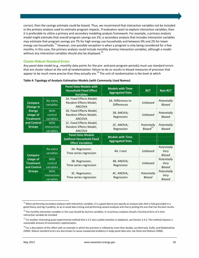
May 2012 www.seeaction.energy.gov 26
correct, then the savings estimate could be biased. Thus, we recommend that interaction variables not be included in the primary analysis used to estimate program impacts. If evaluators want to explore interaction variables, then it is preferable to utilize a primary and secondary modeling analysis framework. For example, a primary analysis model might estimate that overall program savings are 2%; a secondary analysis that includes interaction variables may estimate that program savings are 7% for high energy use households and between 0% and 2% for lower energy use households.
75 However, one possible exception is when a program is only being considered for a few
months; in this case, the primary analysis could include monthly dummy interaction variables, although a model without any interaction variables should also be displayed.
76
Cluster-Robust Standard Errors Any panel data model (e.g., monthly data points for the pre- and post-program periods) must use standard errors that are cluster robust at the unit of randomization: failure to do so results in biased measures of precision that appear to be much more precise than they actually are.
78 The unit of randomization is the level at which
75 When performing secondary analyses with interaction variables, it is a good idea to pre-specify an analysis plan that is fully grounded in a good theory and log it publicly, so as to avoid data mining and performing several analyses and cherry picking the one that has the best results.
76 The monthly interaction variables in this case should be dummy variables; in no primary analyses should a functional form of a time interaction variable be included.
77 For another interesting quasi-experimental method that is 3.5 stars (called variation in adoption), see Section 2.4.3. This method requires a reasonable amount of econometric sophistication.
78 For a description of this effect with an example in which the precision is inflated by more than double, see Bertrand, Duflo, and Mullainathan (2004). Robust standard errors are also known to cause unexpected problems in large panel data sets; see Stock and Watson (2006).
Table 4: Typology of Analysis Estimation Models (with Commonly Used Names)
Panel Data Models with Household-Fixed Effect
Variables
Models with Time-Aggregated Data
RCT Non-RCT
Compare Change in
Energy Usage of
Treatment and Control
Groups
No extra variables
1A. Fixed Effects Model; Random Effects Model;
ANCOVA
2A. Difference-in-Differences
Unbiased Potentially
Biased
With control
variables
1B. Fixed Effects Model; Random Effects Model;
ANCOVA
2B. ANOVA; Regression
Unbiased Potentially
Biased
With interaction variables
1C. Fixed Effects Model; Random Effects Model;
ANCOVA
2C. ANOVA; Regression
Potentially Biased
77
Potentially Biased
Panel Data Models (without Household-Fixed
Effect Variables)
Models with Time-Aggregated Data
Compare Usage of
Treatment and Control
Groups
No extra variables
3A. Regression; Time-series regression
4A. t-test Unbiased Potentially
Very Biased
With control
variables
3B. Regression; Time-series regression
4B. ANOVA; Regression
Unbiased Potentially
Very Biased
With interaction variables
3C. Regression; Time-series regression
4C. ANOVA; Regression
Potentially Biased
Potentially Very
Biased

May 2012 www.seeaction.energy.gov 27
households were randomly allocated into a control or treatment group. Typically, the level of randomization is the household; thus, standard errors should be clustered at the household level.
79
Clustering standard errors means that the analysis accounts for the fact that 12 months of energy use data from one household is not the same as one month of energy use data from 12 households. In effect, it clusters the 12 months of data in the model so that all 12 months come from one household. This is important because otherwise the model will report standard errors that are biased, which would imply that the estimates are more precise than the data can justify.
For example, a panel data model with standard errors that are not cluster robust may report an estimate of energy savings of 2% with a confidence interval of (0.8%, 3.2%); in reality, with properly calculated cluster-robust standard errors, the estimate is much less precise with a much larger confidence interval of (-0.2%, 4.2%). This example illustrates the importance of clustering standard errors: the first confidence interval would imply that the 2% savings estimate is statistically significant and greater than zero, while the true confidence interval implies that the 2% savings estimate is not statistically significant because the confidence interval includes zero savings.
Table 6. Cluster-Robust Standard Errors: Recommendation
Star Rating Condition
Cluster-robust standard errors or time-aggregated data
Non-cluster-robust standard errors with non-time-aggregated data
79 In the case of a school-based educational program, households may be randomized at the school level (e.g., all households for one school are placed in either the control group or the treatment group), in which case standard errors should be clustered at the school level or in a multi-way fashion. This technique can be easily implemented in the Stata statistical package using the “cluster” command (e.g., “cluster household,” or “cluster school”).
Table 5. Analysis Model Specification Options: Recommendation
Star Rating Condition
If RCT: If Quasi-Experimental:
Panel data model with fixed effects (comparing change in use), with or without control variables, with a primary analysis that does not include interaction variables
a
Time-aggregated data model comparing change in use, with or without control variables, with a primary analysis that does not include interaction variables
a
Model comparing use (not change in use), with or without control variables, with a primary analysis that does not include interaction variables
a
Any model with a primary analysis that includes interaction variables
a
a Interaction variables should not be included in the primary analysis that assesses the overall program impact, but could be
included in secondary analyses. If necessary from a finacial or regulatory standpoint, the primary analysis could include a model specification that contains time-based, dummy interaction variables in addition to a specification that does not include interaction variables.
Not Advisable
Not Advisable
Not Advisable Not Advisable

May 2012 www.seeaction.energy.gov 28
Equivalency Check Because the degree to which a savings estimate is unbiased depends on how similar the control group is to the treatment group (see Section 2), an important part of the analysis is validating that the two groups are equivalent. This is done by testing whether households in the treatment group have characteristics that are statistically similar to those in the control group (also called a balanced treatment/control check or a randomization check if the method is an RCT). Evaluators should use professional judgment to decide what characteristics need to be tested; possible tests include monthly or yearly pre-program energy use, distribution of pre-program energy use, geographic location, dwelling characteristics (e.g., square footage), demographic characteristics (e.g., age, income), psychographic characteristics (e.g., opinions) and any other baseline covariates for which data is available. This should be done whether the program is designed as an RCT or a quasi-experiment.
80
3.2.3 Issue E: Standard Errors and Statistical Significance
An estimate of program impact savings should not be accepted if it is not sufficiently precise. Stated another way, the savings estimates are too risky to accept if there is too high a chance that the true program savings do not satisfy the required threshold level (e.g., they should not be accepted if there is too big a risk that the savings are not greater than zero or if there is too big a risk that they are not sufficient to support a cost-effectiveness screening requirement). To ensure a level of precision that is considered acceptable in behavioral sciences research, a null hypothesis (i.e., a required threshold such as the level or percentage of energy savings needed for the benefits of the program to be considered cost-effective) should be established, and the program savings estimate should be considered acceptable (and the null hypothesis should be rejected) if the estimate is statistically significant at the 5% level or lower.
This means that there is a 5% (or lower) chance that the
80 With RCTs, one option to ensure that the randomization is balanced is to perform multiple randomizations (e.g., 1,000), do an equivalency check for each one, and then choose the randomization that is the most balanced (e.g., that has the smallest maximum t-statistic out of all of the compared baseline covariates). For an example of an equivalency check, see: Opinion Dynamics Corporation (2011).
REAL WORLD EXAMPLE
Estimation Methods: Connexus Energy’s Opower Energy Efficiency Pilot Program
Method: Panel Data Model
with Fixed Effects
Method: Clustered Standard
Errors
Method: Equivalency Check
Connexus Energy, a utility in Minnesota, partnered with Opower to launch a residential energy efficiency program using home energy reports (HERs) in 2009. Allcott (2011) evaluated the program and estimated the energy savings resulting from the program. Allcott performed an equivalency check and used a panel data model with household-fixed effects and used standard errors clustered at the household level. The model also included control variables in the form of 12 month-of-year specific dummy variables (i.e., one variable indicating whether or not the month was January, one indicating whether or not the month was February, etc.).
Allcott, H. 2011. “Social Norms and Energy Conservation.” Journal of Public Economics.
Table 7. Equivalency Check: Recommendation
Star Rating Condition
An equivalency check is performed with household energy usage profiles as well as demographic, geographic, and other household characteristics.
An equivalency check is performed with household energy usage profiles.
An equivalency check is not performed.
Not Advisable

May 2012 www.seeaction.energy.gov 29
savings estimate is considered to acceptably satisfy the required threshold level when in fact the true savings actually do not satisfy the requirement (i.e., a 5% chance that the null hypothesis is rejected when in fact the null hypothesis is true).
81,82,83
One way to increase the precision of an estimate is by adding more information to the analysis model (e.g., by increasing the number of households that are in the control and treatment groups). Another option is to change the type of analysis by: (1) moving to a model that estimates the change in energy use for both the treatment and control rather than only the energy use for both groups; (2) moving to a panel data model rather than an aggregated data model; or (3) adding extra control variables (see Section 3.2.2 for more details on analysis models).
3.2.4 Issue F: Excluding Data from Households that Opt Out or Close Accounts
Typical ways that study populations are segmented are by excluding those that opt out of the program or those that closed their accounts. Households that opt out should never be excluded from the dataset; they should be included as part of the treatment group to avoid selection bias (see Section 2.3.1). If households that opt out of a program are excluded from the treatment group, then the treatment group no longer contains the same types of households as the control group (because these people cannot be excluded from the control group). As a result, an analysis that excludes households that opt out is comparing two fundamentally different groups, which may result in major selection bias and thus any resulting estimate of energy savings may be biased.
84
While an analysis that includes the households that opt out will yield an unbiased estimate of program impacts for all households in the treatment group (both those that receive the program and those that opt out, called the intent-to-treat group), another effect of interest is the program impacts for all households in the treatment group that did not opt out, and that therefore received the program (i.e., the effect of the program on the treated group). In order to calculate an unbiased estimate of the effect of the program on those that did not opt out, the program impact should first be estimated including the opt-out households as part of the treatment group. Then, the estimate should be divided by the percentage of households that did not opt out. For example, if the estimate of the overall savings is 2% for all households in the treatment group, but 20% of the households opted out of the program, then the estimate, then the estimate of the effect of the program on the treated households that do not opt out is higher (i.e., 2.5%, which is 2% divided by 80%).
81 For example, if the desired test is whether or not a program’s energy savings satisfy a cost-effectiveness threshold requirement, the null hypothesis would be that the energy savings do not satisfy the requirement. Then, if the savings estimate is statistically significant at 4%, it means that there is only a 4% chance that the savings do not satisfy the requirement (and a 96% chance that the savings do satisfy the requirement); because it is less than 5%, the savings estimate should be considered acceptable.
82 Note that these recommendations apply to the measurements of savings and have nothing to do with the sample size selection requirement typically referenced in energy efficiency evaluations. Sample size selection is usually required to have 10–20% precision with 80–90% confidence and may be referred to as “90/10” or “80/20”. A 5% level of statistical significance does not mean “95/5”.
83 While a savings estimate that is not statistically significant at 5% should not be accepted, this does not conclusively mean that the true program savings do not reach the required threshold. It is possible that there were not enough households in the study population to see an effect. In this situation, the evaluator may recommend increasing the sample size to obtain a more definitive estimate of program effectiveness.
84 When a program is designed, the expected opt-out rate should be taken into account so that the correct number of households can be placed in the treatment and control groups.
Table 8. Statistical Significance: Recommendation
Star Rating Condition
An estimate that is statistically significant at 5% should be accepted and the null hypothesis (or required threshold) should be transparently defined.
An estimate that is statistically significant at greater than 5% should not be accepted.
Not Advisable
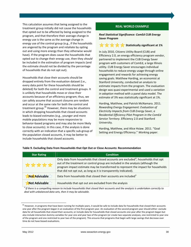
May 2012 www.seeaction.energy.gov 30
This calculation assumes that being assigned to the treatment group initially did not cause the households that opted out to be affected by being assigned to the program, and that therefore their average change in energy use is the same as the average change in energy use of the control group (e.g., if the households are angered by the program and retaliate by opting out and using more energy than they otherwise would have). If the program does cause the households that opted out to change their energy use, then they should be included in the estimation of program impacts (and the estimate should not be divided by the percentage of households that do not opt out).
Households that close their accounts should be dropped entirely from the evaluation dataset (i.e., every data point for these households should be deleted) for both the control and treatment groups. It is unlikely that households move or close their accounts because of an efficiency program; thus, we can safely assume that account closures are random and occur at the same rate for both the control and treatment group.
85 However, there may be situations
in which dropping households that closed accounts leads to biased estimates (e.g., younger and more mobile populations may be more responsive to behavior-based programs and may also be more likely to close accounts). In this case, if the analysis is done correctly with an indication that a specific sub-group of the population closed accounts, it may be better to include households that closed accounts.
85 However, in programs that have been running for multiple years, it would be safe to include data for households that closed their accounts one year after the program began in an evaluation of the first program year. An evaluation of the second program year should either: exclude data for all households that closed their accounts; or include data for households that closed accounts one year after the program began but also include interaction dummy variables for year one and year two of the program (or create two separate analyses, one restricted to year one of the program and one restricted to year two of the program). This ensures that programs that begin with large savings that decrease over time do not have biased evaluations.
Real Statistical Significance: ComEd CUB Energy Saver Program
Statistically significant at 1%
In July 2010, Citizens Utility Board (CUB) and Efficiency 2.0, an energy efficiency program vendor, partnered to implement the CUB Energy Saver program with customers of ComEd, a large Illinois utility. CUB Energy Saver encourages individual households to reduce energy usage through online engagement and rewards for achieving energy saving goals. Matthew Harding, an economist at Stanford University, conducted an analysis to estimate impacts from the program. The evaluation design was quasi-experimental and used a variation in adoption method with a panel data model. The estimate of 3% was statistically significant at 1%.
Harding, Matthew, and Patrick McNamara. 2011. Rewarding Energy Engagement: Evaluation of Electricity Impacts from CUB Energy Saver, a Residential Efficiency Pilot Program in the ComEd Service Territory. Efficiency 2.0 and Stanford University.
Harding, Matthew, and Alice Hsiaw. 2011. “Goal Setting and Energy Efficiency.” Working paper.
Table 9. Excluding Data from Households that Opt Out or Close Accounts: Recommendation
Star Rating Condition
Only data from households that closed accounts are excludeda; households that opt
out of the treatment or control group are included in the analysis (although the program impact estimate may be transformed to represent the impact for households that did not opt out, as long as it is transparently indicated).
Data from households that closed their accounts are included
a
Households that opt out are excluded from the analysis
a If there is a compelling reason to include households that closed their accounts and the analysis is undertaken correctly to
deal with unbalanced data sets, then it may be advisable.
REAL WORLD EXAMPLE
Not Advisable
Not Advisable

May 2012 www.seeaction.energy.gov 31
3.2.5 Issue G: Accounting for Potential Double Counting of Savings
Behavior-based programs are a relatively new program concept that is being pilot tested and implemented by many program administrators. In many states, behavior-based efficiency programs are offered in an environment where the administrator already has many other residential efficiency programs. Thus, the evaluation questions are often framed in terms of how much additional savings are gained from behavior-based programs and at what program cost. In this environment, there is the possibility that more than one program could claim savings from installation of the same measure; thus, program administrators, evaluators, and regulatory staff need to address issues related to potential double counting of savings (e.g., a CFL rebate program, an education program, and a behavioral program might all claim savings for installation of CFLs). This issue may arise if or when program administrators add up the savings for each program to report overall portfolio savings achieved for compliance with an Energy Efficiency Resource Standard (EERS), as part of a program administrator’s claim for shareholder incentives or lost revenue recovery mechanism, or in an annual energy efficiency report to a state regulatory commission.
One advantage of a behavior-based efficiency program that is evaluated with a treatment and control group is that it provides a method for at least partial accounting for this phenomenon. This is because double-counted savings are equal to the amount of savings claimed by the other program(s) for households in the treatment group minus the amount of savings claimed by the other program(s) for households in the control group.
86,87 For example (see
Figure 14), assuming that the control and treatment groups have the same number of households, if customers in the treatment group used 100 more refrigerator rebates than customers in the control group and each high-efficiency refrigerator is estimated to save 500 kWh per year, then the double-counted savings are 50,000 kWh/year (i.e., the savings attributable to this measure that are claimed by both the behavioral-based efficiency program and the refrigerator rebate program).
For programs in which efficiency measures can be tracked to a specific household (e.g., installation of insulation by a contractor), double-counted savings can be directly determined. For programs in which efficiency measures cannot be tracked to specific households (e.g., upstream CFL rebates), determining double-counted savings in a rigorous way is a much more serious challenge. One approach involves using customer surveys to estimate measures installed by customers through the upstream efficiency program; however, surveys typically do not achieve very high response rates and may be subject to selection bias.
88 There is a need for additional research
that explores other evaluation approaches and strategies that address this issue of accounting for potential double-savings for efficiency programs where measures cannot be tracked to specific households.
86 This is true for both RCT and quasi-experimental approaches. However, because RCT evaluation designs may result in savings estimates that are more valid than quasi-experimental methods, the estimate of the magnitude of the double-counted savings is also likely to be more valid with RCT approaches than quasi-experimental approaches (and we therefore give quasi-experimental approaches fewer stars).
87 For a report that discusses challenges in measuring double-counted savings as well as other issues, see Smith, Brian, and Sullivan (2011).
88 For an example of estimating savings claimed by other programs for households in the treatment and control groups of the behavior-based program, see Dougherty, Dwelley, Henschel, and Hastings (2011).
REAL WORLD EXAMPLE
Excluding Data from Households that Opt Out or Drop Out: Puget Sound Energy’s Home Energy Reports Program
Method: Excluding Data
KEMA’s “20 Month Impact Evaluation” (KEMA 2010) of the 2008 Puget Sound Energy (PSE) Home Energy Reports (HER) pilot included households that opted out of the program in the analysis. Three types of households were removed from the analysis: (1) a small number of households that did not have usable zip codes; (2) one zip code in the treatment group that had not been included in the randomized selection process; (3) the roughly 10% of the study households that moved or changed accounts during the 20 months since the program began.
KEMA. 2010. Puget Sound Energy’s Home Energy Reports Program: 20 Month Impact Evaluation. Madison, WI.
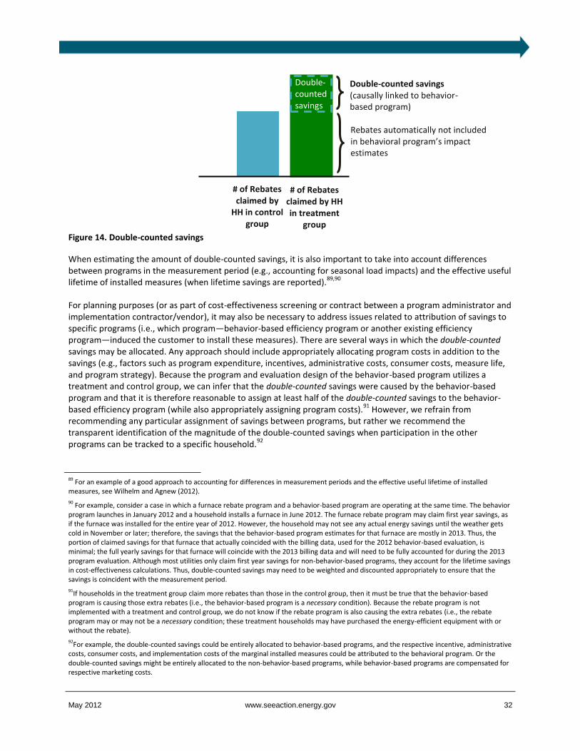
May 2012 www.seeaction.energy.gov 32
When estimating the amount of double-counted savings, it is also important to take into account differences between programs in the measurement period (e.g., accounting for seasonal load impacts) and the effective useful lifetime of installed measures (when lifetime savings are reported).
89,90
For planning purposes (or as part of cost-effectiveness screening or contract between a program administrator and implementation contractor/vendor), it may also be necessary to address issues related to attribution of savings to specific programs (i.e., which program—behavior-based efficiency program or another existing efficiency program—induced the customer to install these measures). There are several ways in which the double-counted savings may be allocated. Any approach should include appropriately allocating program costs in addition to the savings (e.g., factors such as program expenditure, incentives, administrative costs, consumer costs, measure life, and program strategy). Because the program and evaluation design of the behavior-based program utilizes a treatment and control group, we can infer that the double-counted savings were caused by the behavior-based program and that it is therefore reasonable to assign at least half of the double-counted savings to the behavior-based efficiency program (while also appropriately assigning program costs).
91 However, we refrain from
recommending any particular assignment of savings between programs, but rather we recommend the transparent identification of the magnitude of the double-counted savings when participation in the other programs can be tracked to a specific household.
92
89 For an example of a good approach to accounting for differences in measurement periods and the effective useful lifetime of installed measures, see Wilhelm and Agnew (2012).
90 For example, consider a case in which a furnace rebate program and a behavior-based program are operating at the same time. The behavior program launches in January 2012 and a household installs a furnace in June 2012. The furnace rebate program may claim first year savings, as if the furnace was installed for the entire year of 2012. However, the household may not see any actual energy savings until the weather gets cold in November or later; therefore, the savings that the behavior-based program estimates for that furnace are mostly in 2013. Thus, the portion of claimed savings for that furnace that actually coincided with the billing data, used for the 2012 behavior-based evaluation, is minimal; the full yearly savings for that furnace will coincide with the 2013 billing data and will need to be fully accounted for during the 2013 program evaluation. Although most utilities only claim first year savings for non-behavior-based programs, they account for the lifetime savings in cost-effectiveness calculations. Thus, double-counted savings may need to be weighted and discounted appropriately to ensure that the savings is coincident with the measurement period.
91If households in the treatment group claim more rebates than those in the control group, then it must be true that the behavior-based program is causing those extra rebates (i.e., the behavior-based program is a necessary condition). Because the rebate program is not implemented with a treatment and control group, we do not know if the rebate program is also causing the extra rebates (i.e., the rebate program may or may not be a necessary condition; these treatment households may have purchased the energy-efficient equipment with or without the rebate).
92For example, the double-counted savings could be entirely allocated to behavior-based programs, and the respective incentive, administrative costs, consumer costs, and implementation costs of the marginal installed measures could be attributed to the behavioral program. Or the double-counted savings might be entirely allocated to the non-behavior-based programs, while behavior-based programs are compensated for respective marketing costs.
# of Rebates claimed by
HH in control group
# of Rebates claimed by HH in treatment
group
Double-counted savings (causally linked to behavior-based program)
Figure 14. Double-counted savings
Rebates automatically not included in behavioral program’s impact estimates
Double-counted savings
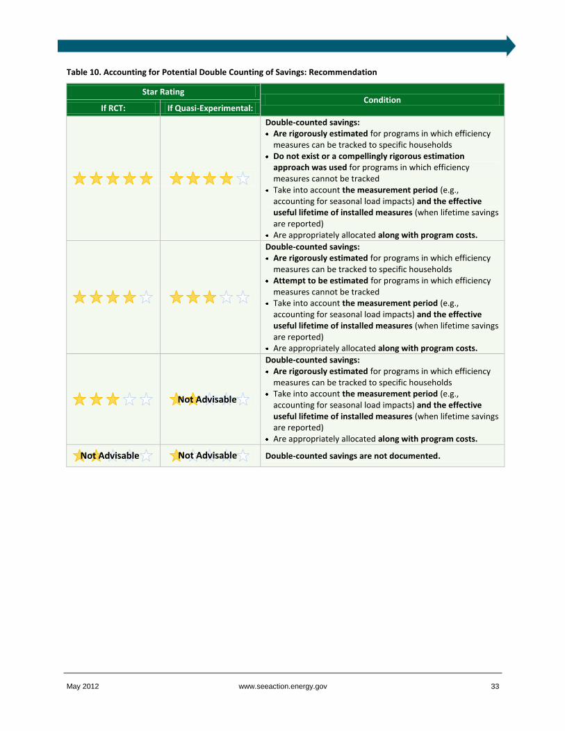
May 2012 www.seeaction.energy.gov 33
Table 10. Accounting for Potential Double Counting of Savings: Recommendation
Star Rating Condition
If RCT: If Quasi-Experimental:
Double-counted savings: Are rigorously estimated for programs in which efficiency
measures can be tracked to specific households Do not exist or a compellingly rigorous estimation
approach was used for programs in which efficiency measures cannot be tracked
Take into account the measurement period (e.g., accounting for seasonal load impacts) and the effective useful lifetime of installed measures (when lifetime savings are reported)
Are appropriately allocated along with program costs.
Double-counted savings: Are rigorously estimated for programs in which efficiency
measures can be tracked to specific households Attempt to be estimated for programs in which efficiency
measures cannot be tracked Take into account the measurement period (e.g.,
accounting for seasonal load impacts) and the effective useful lifetime of installed measures (when lifetime savings are reported)
Are appropriately allocated along with program costs.
Double-counted savings: Are rigorously estimated for programs in which efficiency
measures can be tracked to specific households Take into account the measurement period (e.g.,
accounting for seasonal load impacts) and the effective useful lifetime of installed measures (when lifetime savings are reported)
Are appropriately allocated along with program costs.
Double-counted savings are not documented.
Not Advisable
Not Advisable Not Advisable

May 2012 www.seeaction.energy.gov 34
REAL WORLD EXAMPLE
Accounting for Potential Double Counting of Savings: Puget Sound Energy’s Home Energy Reports Program
Method: Accounting for Potential Double Counting of Savings
KEMA conducted a “20 Month Impact Evaluation” (KEMA 2010) of the 2008 Puget Sound Energy (PSE) Home Energy Reports (HER) pilot. The evaluation included an examination of tracking data from other PSE energy efficiency programs. The HER includes energy saving tips and encourages participating households to change habitual behaviors and take advantage of other PSE programs (e.g., appliance rebates) so the evaluation noted the potential for double counting savings if the HER drives participation in other programs. However, the RCT design allowed evaluators to examine whether there appeared to be any systemic increase in participation in other programs among the treatment group relative to the control group.
Participation information for the PSE rebate program was gathered for all households in both the participant and control groups of the HER pilot. Rebate information from January 2007 to June 2010 was examined. KEMA used two different methodologies to estimate the amount of detected savings from the HER program that could potentially be double counted: a time of participation method and a load shape-allocated method. KEMA found that preliminary examination of the data showed little evidence that the HERs increased participation in other programs among the treatment households.
KEMA. 2010. Puget Sound Energy’s Home Energy Reports Program: 20 Month Impact Evaluation. Madison, WI.
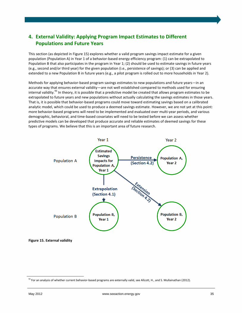
May 2012 www.seeaction.energy.gov 35
4. External Validity: Applying Program Impact Estimates to Different Populations and Future Years
This section (as depicted in Figure 15) explores whether a valid program savings impact estimate for a given population (Population A) in Year 1 of a behavior-based energy efficiency program: (1) can be extrapolated to Population B that also participates in the program in Year 1; (2) should be used to estimate savings in future years (e.g., second and/or third year) for the given population (i.e., persistence of savings); or (3) can be applied and extended to a new Population B in future years (e.g., a pilot program is rolled out to more households in Year 2).
Methods for applying behavior-based program savings estimates to new populations and future years—in an accurate way that ensures external validity—are not well established compared to methods used for ensuring internal validity.
93 In theory, it is possible that a predictive model be created that allows program estimates to be
extrapolated to future years and new populations without actually calculating the savings estimates in those years. That is, it is possible that behavior-based programs could move toward estimating savings based on a calibrated analytic model, which could be used to produce a deemed savings estimate. However, we are not yet at this point: more behavior-based programs will need to be implemented and evaluated over multi-year periods, and various demographic, behavioral, and time-based covariates will need to be tested before we can assess whether predictive models can be developed that produce accurate and reliable estimates of deemed savings for these types of programs. We believe that this is an important area of future research.
Figure 15. External validity
93 For an analysis of whether current behavior-based programs are externally valid, see Allcott, H., and S. Mullainathan (2012).

May 2012 www.seeaction.energy.gov 36
Figure 16. Applicability of savings estimates from one population to another in the initial program year (random
sample)
In the following sections, we generally recommend that program impacts should not be extrapolated or extended to new years and new populations in situations for which the outcome has significant financial and regulatory implications (e.g., determining incentives to be paid to a program administrator or compensating implementation contractors for program costs). However, a well-designed RCT program may produce an estimate that is helpful in deciding whether or not to scale up a program. For example, a program that estimates negative savings should probably not be scaled up, whereas a program that develops savings estimates that indicate that the program is cost effective could be considering for scaling up (although it is not valid to assume that the scaled up program will produce the same level of savings in future years).
4.1 Extrapolation to a Different Population in Year 1
This section explores the possibility of extrapolating a valid savings impact estimate for one population to another population during the same year. As depicted in Figure 16 and Figure 17, this is a situation in which there are two populations (A and B) that a program administrator wishes to enroll in the program. Population A has a treatment and control group and their energy use data are measured in order to estimate a program savings impact. However, perhaps due to budgetary constraints, Population B’s energy use is not measured and evaluated, and all households in Population B receive the program (i.e., the entire population is a treatment group). The question of interest is under what conditions the program savings impacts for Population A can be extrapolated and applied to Population B.
In this situation, the external validity of the estimate depends on the similarity of Population A to Population B. There are two cases to consider. In Scenario 1 (see Figure 16), Population A is a random sample of an original population pool containing Population A and B. For this scenario, because the sample is random, Population A and B should have statistically identical observable and unobservable characteristics. If the program enrollment

May 2012 www.seeaction.energy.gov 37
method is the same for the initial and new populations (i.e., opt-in or opt-out), the estimated savings impacts from the initial population (A) can be directly applied to the new population (B) under this scenario.
94
In Scenario 2 (see Figure 17), Population B is a different population than A (e.g., Population A has many more high energy users than Population B, Population A is in a different neighborhood than Population B, or Population A was recruited using an opt-out enrollment strategy while customers in Population B had to opt in to the program). Because Populations A and B have different observable and unobservable characteristics, we do not recommend applying the savings impacts estimated for Population A to Population B under this scenario.
95
Figure 17. Applicability of savings estimates from one population to another (different population)
Table 11. Extrapolation of Impact Estimates from Population A to B: Recommendation
Star Rating Condition
Impact estimates for Population A are extrapolated to Population B, where A was a random sample from Population A + B, and the same enrollment method was used for both populations (opt-in or opt-out).
Impact estimates for Population A are extrapolated to B, where B has very similar characteristics to A, and the same enrollment method was used for both populations (opt-in or opt-out).
Impact estimates for Population A are extrapolated to B, where Population B has different characteristics than Population A.
Impact estimates for Population A are extrapolated to Population B, where Population A was recruited with a different enrollment method than B .
94 However, if energy data for the Population B is obtainable, then it is always better to estimate the program impacts with the entire population.
95 For planning purposes and cost-effectiveness screening, it may be useful and appropriate to determine the degree to which Population A is similar to B in order to establish and ex ante estimate of savings that can be used for program screening purposes (e.g., if Population A is in a neighboring county to B and has similar demographic and energy use characteristics, then B might be expected to show similar savings).
Not Advisable
Not Advisable

May 2012 www.seeaction.energy.gov 38
4.2 Persistence of Savings
An important issue for many stakeholders is whether energy savings from behavior-based programs continue over time (i.e., whether they persist beyond the initial program year). There are at least two different situations for which evaluators may assess persistence of savings:
The program provides periodic or continuous intervention (e.g., information and/or feedback) and customers may or may not continue to respond as they did initially and thus savings may erode, or potentially increase, during the program period.
The program stops providing the intervention and thus savings may persist or erode in the absence of the intervention.
Because the subject programs are based primarily on changing energy behaviors or practices, there is concern that savings may not last or persist for many years or may be less predictable over time as compared to savings from installation of high-efficiency equipment and appliances. There is very limited evidence from a few behavior efficiency programs that document savings for programs after the first year. This is at least in part because residential behavior-based programs have either only been offered or evaluated for the initial year. Thus, there is not enough evidence to draw any definitive conclusions.
96 This is complicated by the fact that persistence may not
be uniform across different designs and types of behavior-based efficiency programs; it may depend on specific program elements, such as marketing channels (e.g., internet, letters, face to face), timing or consistency of feedback (e.g., monthly or real-time feedback), the type of customer segment that is targeted, or other factors. Persistence of savings may also be influenced by external conditions that change from year to year (e.g., economic or weather conditions, other concurrent energy efficiency programs, the political climate, and popular culture).
From a planning perspective, it would be useful to know how the savings impacts of a typical behavior-based program change over time, which could be considered in cost-effectiveness screening. From an impact evaluation perspective, it would be useful to know whether a program must be evaluated after every year or whether the results from the first year (or first few years’) can reasonably be extrapolated to future years (e.g., if Year 1 had 2% savings, can we assume that savings for Years 2 and 3 will also be 2%?).
97
More evidence on persistence of energy savings in behavior-based programs will become available as the new generation of programs mature and are evaluated over the next several years. Once a program has been running for several years and valid program impact estimates have been calculated in each of those years, it may be possible to evaluate the program every two or three years. However, at this time, we do not recommend applying
96 Skumatz (2009) states: “Probably the single biggest gap in lifetime studies is the virtual non-existence of studies examining the retention of education, training, and behavior-focused ‘measures’ ”. Skumatz cites an early study by Harrigan and Gregory (1994) that found 85-90% of savings were retained in an educational portion of a weatherization program. Allcott (2011) found “no evidence in decline in the treatment effects” after two years for three programs that sent Home Energy Reports by mail.
97 Saving impact estimates for an initial year could also be extrapolated to future years based on an assumed decay function that would reflect the fact that some/many customers will not continue energy-efficient behaviors or practices in the absence of an ongoing program (e.g., initial year savings of 2% are assumed to decrease by 10-15% in subsequent years through Year 4).
RECOMMENDATION
A control group should be maintained for every year and each population for which program impact estimates are calculated.
Table 12. Persistence of Savings: Recommendation
Star Rating Condition
A control group is maintained for every year in which program impacts are estimated, and the program is evaluated ex-post every year initially and every few years after the program has been running for several years.
Program impact estimates are directly applied from the first year(s) of the program to future years without measuring and analyzing energy use data.
Not Advisable

May 2012 www.seeaction.energy.gov 39
results from one year directly to another year and foregoing evaluation entirely. Note that this implies that a control group must be maintained for every year in which program impact estimates are calculated and that the program treatment group therefore cannot be expanded to every household in a given population.
98 It is also
possible that at some point behavior-based programs could move to an EM&V approach that uses predictive models (see Section 4.4 for a brief discussion of this issue).
4.3 Applying Savings Estimates to a New Population of Participants in Future Years
If a pilot behavior-based efficiency program is successful, then program administrators may want to extend the program to additional populations over time. In this case, it may be important to assess whether the initial program’s impact estimates can be applied to the expanded program. There are two contexts for which the validity of the estimates may be relevant: (1) program planning or cost-effectiveness screening; and (2) claiming energy savings credits after the program is implemented.
For planning purposes, the degree to which the initial population is similar to the new population and future years are similar to initial years determines the extent to which the initial savings estimates can be regarded as an ex ante savings estimate and extrapolated to this new situation. However, for the purpose of claiming savings credits, for reasons discussed in Sections 4.1 and 4.2, we do not recommend directly applying program savings impact estimates from an initial program to an expanded program with a new population in a future year. Instead, we recommend creating and maintaining a new control and treatment group, and evaluating the expanded program using the methods described in this report.
4.4 Using Predictive Models to Estimate Savings
In theory, it is possible that a predictive model could be created in which the first few years of measured data are input into the model along with the conditions that occurred in the year that is being predicted (e.g., weather and economic conditions), and the result is a prediction of the estimated energy savings for that predicted year. Actual estimated results are more accurate, although a predictive model is much cheaper to implement (once it is created).
We believe that future research may lead to the creation of a rigorous predictive model that controls for a sufficiently rich set of demographic and behavioral covariates to a very large extent. However, we are not currently aware of such a model and cannot predict what such a model would include. Therefore, rather than prescribe a method for creating a predictive model, we recommend a set of criteria that any future predictive model must meet in order to be credible. In this section, we focus on the validity of a predictive model for the purposes of claiming energy savings credits for a program that has not been evaluated with measured data.
99 We refer to
measured years as the years for which the data were collected and evaluated, and the predicted years as the years that are not measured but are predicted by a model.
98 However, the control group does not have to be half of the population, it could be far less. It is only necessary to keep a control group that is sufficiently large to yield statistical significance of the savings estimate (taking into account closed accounts and other attrition). If the control group is found to be larger than needed to yield statistical significance, then some households in the control group could be offered the program. For an excellent guide to implementing programs, including guidelines for calculating the number of households needed in the study population in order to get a precise estimate, see Chapter 4 of Duflo, Glennerster, and Kremer (2007). See EPRI (2010) for a comprehensive guide to implementing energy information feedback pilots that is applicable to non-feedback programs as well.
99 Predictive models used for planning and cost-effectiveness screening purposes would have a lower criteria requirement.

May 2012 www.seeaction.energy.gov 40
Table 13. Applying Savings Estimates to an Extended Population: Recommendation
Star Rating
Condition Program Planning or Cost-Effectiveness
Screening Purposes
Claiming Savings Credit after Program
Implementation
A control group is created and maintained for every population in the expanded program and each year in order to create impact estimates. Program impact estimates are directly applied from the initial program with Population A in Year 1 to the extended program with Population B in Year 2, in the case that:
Population A was a random sample from Population A + B The enrollment method was the same for Populations A and
B (opt-in or opt-out) Year 2 has similar conditions to Year 1.
Population B has very similar characteristics to Population A The enrollment method was the same for Populations A and
B (opt-in or opt-out) Year 2 has similar conditions to Year 1.
Population B has different characteristics than Population A
Population B was recruited with a different enrollment
method than Population A (opt-in or opt-out).
Year 2 has different conditions than Year 1 (e.g., the program has changed or stopped, there are different economic or weather conditions, other concurrent energy efficiency programs, political climate, etc.).
4.4.1 Internal Conditions
Internal conditions are conditions that can be controlled by the utility, such as the way the program is implemented. Ideally, these internal conditions should remain the same in the predicted years as they were in the initial measured years. For example, the program should not be discontinued, the population should remain unchanged, and no major changes should be made to the program (or to other programs offered by the program administrator).
4.4.2 External Conditions
External conditions are conditions that are beyond the control of the utility but which might affect estimates of the program’s impact. These include factors such as economic conditions, weather conditions, social norms, costs and availability of efficiency products and services, other efficiency strategies (e.g., new appliance standard), and other conditions that may affect the energy behavior of households. Ideally, the predictive model should attempt to account for these external conditions. In order to accurately predict future years, the model should be calibrated with initial data that spans a range of different values for each of the external conditions. For example, if the predicted year has temperatures that are 20 degrees higher than temperatures that the model has been calibrated with, then the predictive model will likely not be accurate.
4.4.3 Risk Adjustment
From a policymaker’s or regulator’s perspective, it is likely more risky to accept estimates of savings based on a predictive model than on measured data from an RCT evaluation. One option is to adjust and de-rate the savings estimates produced by the predictive model to account for additional uncertainties and risks. Another option is that program administrators and regulators consider de-rating the predictive model’s estimate of energy savings to
Not Advisable
Not Advisable
Not Advisable Not Advisable
Not Advisable Not Advisable
Not Advisable Not Advisable

May 2012 www.seeaction.energy.gov 41
the lower bound of the 95% confidence interval. For example, if the savings estimate is 2% with a confidence interval of (0.8%, 2.2%), then a program administrator could claim annual savings of 0.8% for a behavior-based efficiency program for an agreed upon number of years (e.g., Years 2 and 3). If that option were not attractive, then the program administrator could perform an RCT evaluation that would form the basis for a savings claim in Years 2 and 3.
4.4.4 Model Validation
The model should be validated with actual data before it is used, and then should be validated every few years. To validate the model, the model should make a prediction of the estimated program savings for a year in which the data have yet to be collected (an ex-ante prediction). Once the data are collected and the estimated energy savings are measured from the data, then the measured estimate of savings should be compared to the predicted estimate of savings (it is verified ex-post). If the predicted estimate is the same as or very close to the measured estimate (e.g., if it is within the 99% confidence interval), then the predictive model may be able to be used in future years. However, each year should be evaluated to determine if the external conditions in the predicted year are within the range of the measured years (as discussed above).
The model should also be validated (ex-ante predictions are verified ex-post) with measured estimates every few years to ensure that savings predictions are still accurate. If they are not, the predictive model must be recalibrated and tested.
Table 14. Predictive Model: Recommendation
Star Rating Condition
The predictive model is calibrated with many years of measured program data; the internal conditions remain unchanged (e.g., the program continues unchanged); external conditions in the predicted years are similar to conditions that occurred in measured years; the model is validated (i.e., it makes a prediction ex-ante that is verified ex-post); and savings estimates from the model are risk-adjusted (i.e., claimed savings are the lower bound of the 95% confidence interval).
Any of the above is not true. Not Advisable
May 2012 www.seeaction.energy.gov 42
References
Allcott, H. 2011a. “Rethinking Real-time Electricity Pricing.” Resource and Energy Economics.
Allcott, H. 2011b. “Social Norms and Energy Conservation.” Journal of Public Economics.
Allcott, H., and S. Mullainathan. 2010. “Behavior and Energy Policy.” Science 327 (5970): 1204.
Allcott, H., and S. Mullainathan. 2012. “External Validity and Partner Selection Bias.” NBER Working Paper.
Angrist, J. D, and J. S Pischke. 2008. Mostly Harmless Econometrics: An Empiricist’s Companion. Princeton Univ Pr.
Bertrand, M., E. Duflo, and S. Mullainathan. 2004. “How Much Should We Trust Differences-in-Differences Estimates?” Quarterly Journal of Economics 119 (1): 249–275.
Consortium for Energy Efficiency. 2011. CEE Behavior Program Summary.
Dougherty, Anne, Amanda Dwelley, Rachel Henschel, and Riley Hastings. 2011. Moving Beyond Econometrics to Examine the Behavioral Changes Behind Impacts. IEPEC Conference Paper.
Duflo, E. 2004. “Scaling up and Evaluation.” In Annual World Bank Conference on Development Economics 2004, 341–369.
Duflo, E., R. Glennerster, and M. Kremer. 2007. “Using Randomization in Development Economics Research: A Toolkit.” Handbook of Development Economics 4: 3895–3962.
Efficiency Valuation Organization. 2012. International Performance Measurement and Verification Protocol: Concepts and Options for Determining Energy and Water Savings. www.evo-world.org.
Energy Center of Wisconsin. 2009. Energy Efficiency Guidebook for Public Power Communities. Madison, WI: Energy Center of Wisconsin. www.ecw.org/publicpowerguidebook.
Energy Center of Wisconsin. 2010. Focus on Energy–PowerCost Monitor Study. Madison, WI.
EPRI, Palo Alto, CA. 2010. Guidelines for Designing Effective Energy Information Feedback Pilots: Research Protocols.
Gertler, Paul, Sebastian Martinez, Patrick Premand, Laura B. Rawlings, and Christel M. J. Vermeersch. 2010. Impact Evaluation in Practice. World Bank Publications.
Greene, W., Econometric Analysis, 7th
Ed., Prentice Hall, 2011.
Haley, B., Mahoney, A. 2011. Overview of Residential Energy Feedback and Behavior-Based Energy Efficiency. Energy and Environmental Economics, Inc. www.seeaction.energy.gov/pdfs/ customerinformation_behavioral_status_summary.pdf
Harding, Matthew, and Alice Hsiaw. 2011. “Goal Setting and Energy Efficiency.” Working Paper.
Harding, Matthew, and Patrick McNamara. 2011. Rewarding Energy Engagement: Evaluation of Electricity Impacts from CUB Energy Saver, a Residential Efficiency Pilot Program in the ComEd Service Territor. Efficiency 2.0 and Stanford University.
Imbens, G. M, and J. M Wooldridge. 2009. “Recent Developments in the Econometrics of Program Evaluation.” Journal of Economic Literature 47 (1): 5–86.

May 2012 www.seeaction.energy.gov 43
Imbens, G. W, and T. Lemieux. 2008. “Regression Discontinuity Designs: A Guide to Practice.” Journal of Econometrics 142 (2): 615–635.
KEMA. 2010. Puget Sound Energy’s Home Energy Reports Program: 20 Month Impact Evaluation. Madison, WI.
LaLonde, R. J. 1986. “Evaluating the Econometric Evaluations of Training Programs with Experimental Data.” The American Economic Review: 604–620.
Opinion Dynamics Corporation. 2011. Massachusetts Cross-Cutting Behavioral Program Evaluation. Waltham, MA.
Regional Technical Forum. 2011. Guideline for the Development and Maintenance of RTF Savings Estimation Methods. Regional Technical Forum.
Schiller, S. 2011. End-Use Energy Efficiency Evaluation, Measurement and Verification (EM&V) Resources. www.emvwebinar.org/Meeting%20Materials/2011/Energy%20Efficiency%20EMV%20Documents%20Resources%20Spring%202011.pdf.
Schiller, S. 2007. National Action Plan for Energy Efficiency: Model Energy-Efficiency Program Impact Evaluation Guide. Washington, DC: US EPA. www.epa.gov/solar/documents/evaluation_guide.pdf.
Sergici, S, and A Faruqui. 2011. Measurement and Verification Principles for Behavior-Based Efficiency Programs. The Brattle Group, Inc.
Skumatz, Lisa. 2009. Lessons Learned and Next Steps in Energy Efficiency Measurement and Attribution: Energy Savings, Net to Gross, Non-Energy Benefits, and Persistence of Energy Efficiency Behavior. Berkeley, CA: California Institute for Energy and Environment.
Smith, Brian, and Michael Sullivan. 2011. Assessing Energy Savings Attributable to Home Energy Reports. International Energy Program Evaluation Conference.
Stock, J. H, and M. W Watson. 2006. Heteroskedasticity-robust Standard Errors for Fixed Effects Panel Data Regression. National Bureau of Economic Research.
Sullivan, M. J. 2009. “Using Experiments to Foster Innovation and Improve the Effectiveness of Energy Efficiency Programs.” Working Papers on Behavior, California Institute for Energy and Environment, Oakland, March.
TecMarket Works. 2004. The California Evaluation Framework. San Francisco, California: California Public Utilities Commission.
TecMarket Works. 2006. California Energy Efficiency Evaluation Protocols: Technical, Methodological, and Reporting Requirements for Evaluation Professionals. San Francisco, California: California Public Utilities Commission.
Todd, P. E. 2007. “Evaluating Social Programs with Endogenous Program Placement and Selection of the Treated.” Handbook of Development Economics 4: 3847–3894.
Vine, Edward, Michael Sullivan, Loren Lutzenhiser, Carl Blumstein, and Bill Miller. 2011. Experimentation and the Evaluation of Energy Efficiency Programs: Will the Twain Meet? Boston, MA: International Energy Program Evaluation Conference.
Wilhelm, Bobette, and Ken Agnew. 2012. Addressing Double Counting for the Home Energy Reports Program. Puget Sound Energy’s Conservation Resource Advisory Group. https://conduitnw.org/Pages/File.aspx?rid=786.

May 2012 www.seeaction.energy.gov 44
Appendix A: Checklist
This appendix provides a checklist designed to be used as a tool for policymakers, regulators and implementers in order to assess evaluation options and assign a cumulative overall ranking to a program impact evaluation. All program types begin at ‘Start’, and then are diverted to various sets of questions in Chart A-D depending on the evaluation design. The following set of questions, in Chart M, is common to all program types.

SE
E A
ctio
n: E
valu
atio
n, M
eas
ure
me
nt, a
nd
Ve
rificatio
n (E
M&
V) fo
r Be
ha
vio
r-
Ba
se
d E
nerg
y E
fficie
ncy
Pro
gra
ms

>>> To
con
tinu
e, go to
:
Q2
. Ho
w is th
e treatmen
t grou
p co
mp
ared to
th
e con
trol gro
up
? (a) the en
ergy usage d
urin
g th
e pro
gram is co
mp
ared; o
r (b) th
e cha
ng
e in
energy u
se from
at least 12
mo
nth
s of p
re-
pro
gram d
ata to d
urin
g the p
rogram
is co
mp
ared.
Q1
. Wh
at type o
f evaluatio
n d
esign w
as used
?
Start
RC
T
Co
mp
are C
han
ge,
w/ 1
yr d
ata pre-
pro
gram
Ch
art A
Co
mp
are U
sage
Ch
art B
Re
gressio
n
Disco
ntin
uity
Co
mp
are C
han
ge,
w/ 1
yr d
ata pre-
pro
gram
Ch
art C
Co
mp
are U
sage
X
No
t A
dvis-
ab
le
P
rop
en
sity Sco
re
Match
ing
Co
mp
are C
han
ge,
w/ 1
yr d
ata pre-
pro
gram
Ch
art D
Co
mp
are U
sage
X
No
t A
dvis-
ab
le
M
atchin
g, N
on
-P
rop
en
sity
X
No
t A
dvis-
ab
le
Pre
-Po
st C
om
pariso
n
X
No
t A
dvis-
ab
le

>>> R
ating so
far. To co
ntin
ue, go
to:
Q7
. Is the estim
ated savin
gs statistically sign
ificant at 5
%?
Q6
. Do
es the m
od
el inclu
de an
y interactio
n
variables?
Q5
. (Pan
el On
ly) Are all o
f these in
clud
ed?
•A
fixed effect fo
r each h
ou
seho
ld
•A
"Treatmen
t" variable fo
r each h
ou
seho
ld th
at takes the valu
e 1
du
ring tim
es that th
e ho
useh
old
is particip
ating in
the
pro
gram an
d 0
oth
erwise (co
ntro
l grou
p w
ill have all 0
s)
•A
time variab
le that is th
e same fo
r all ho
useh
old
s
Q4
. (Pan
el On
ly) Are th
e stand
ard erro
rs clu
stered ro
bu
st by h
ou
seho
ld (o
r by u
nit o
f ran
do
mizatio
n, if th
e ho
useh
old
is no
t the
level o
f rand
om
ization
)?
Q3
. Is the an
alysis mo
del a p
anel d
ata mo
del
that u
ses man
y data p
oin
ts ove
r time, o
r a tim
e-aggregated m
od
el that u
ses averaged o
r to
taled d
ata?
Ch
art A:
Type o
f evaluatio
n d
esign is R
CT, an
d
analysis co
mp
ares the ch
ange in
energy
use fo
r the treatm
ent gro
up
to th
e chan
ge in
energy u
se for th
e con
trol gro
up
Ch
art A:
RC
T
Pan
el D
ata Mo
de
l
Stand
ard
Errors
Clu
stered
Pro
perly
Form
ulated
No
In
teractio
n
Variab
les
Significan
t at 5
%
(5 stars)
Ch
art M
No
t Sign
ificant
at 5%
Co
nclu
de
: no
t e
no
ugh
evid
en
ce
that p
rogram
cause
s savin
gs
Inclu
de
s In
teractio
n
Variab
les
X
No
t A
dvisa
ble
No
t P
rop
erly Fo
rmu
lated
X
No
t A
dvisa
ble
Stand
ard
Errors
No
t C
lustered
X
No
t A
dvisa
ble
Time
-Aggre
gated
Data
Mo
de
l
con
tinu
e
con
tinu
e
No
In
teractio
n
Variab
les
Significan
t at 5
%
(5 stars)
Ch
art M
No
t Sign
ificant
at 5%
Co
nclu
de
: no
t en
ou
gh
evid
en
ce w
ith th
is mo
de
l th
at pro
gram cau
ses
savings; su
ggest u
sing
pan
el d
ata mo
de
l Inclu
de
s In
teractio
n
Variab
les
X
No
t A
dvisa
ble

>>> R
ating so
far. To co
ntin
ue, go
to:
Q7
. Is the estim
ated savin
gs statistically sign
ificant at 5
%?
Q6
. Do
es the m
od
el inclu
de an
y interactio
n
variables?
Q5
. (Pan
el On
ly) Is this in
clud
ed?
•A
"Treatmen
t" variable fo
r each h
ou
seho
ld th
at takes the
value 1
for h
ou
seho
lds p
articipatin
g in th
e pro
gram (in
the
treatmen
t grou
p) an
d 0
oth
erwise (fo
r ho
useh
old
s in th
e co
ntro
l grou
p)
Q4
. (Pan
el On
ly) Are th
e stand
ard erro
rs clu
stered-ro
bu
st by h
ou
seho
ld (o
r by u
nit o
f ran
do
mizatio
n, if th
e ho
useh
old
is no
t the
level o
f rand
om
ization
)?
Q3
. Is the an
alysis mo
del a p
anel d
ata mo
del
that u
ses man
y data p
oin
ts over tim
e, or a
time
-aggregated m
od
el that u
ses averaged
or
totaled
data?
Ch
art B:
Type o
f evaluatio
n d
esign is R
CT, an
d
analysis co
mp
ares the en
ergy use fo
r the
treatmen
t grou
p to
the en
ergy use fo
r the
con
trol gro
up
(no
t the ch
ange in
use)
Ch
art B:
RC
T
Pan
el D
ata Mo
de
l
Stand
ard
Errors
Clu
stered
Pro
perly
Form
ulated
No
In
teractio
n
Variab
les
Significan
t at 5
%
(4.5
stars) C
hart M
No
t Sign
ificant
at 5%
Co
nclu
de
: no
t en
ou
gh
evid
en
ce th
at pro
gram
cause
s savings; su
ggest
com
parin
g cha
ng
e in
u
se rath
er th
an u
se In
clud
es
Inte
raction
V
ariable
s
X
No
t A
dvisa
ble
No
t P
rop
erly Fo
rmu
lated
X
No
t A
dvisa
ble
Stand
ard
Errors
No
t C
lustered
X
No
t A
dvisa
ble
Time
-Aggre
gated
Data
Mo
de
l
con
tinu
e
con
tinu
e
No
In
teractio
n
Variab
les
Significan
t at 5
%
(4.5
stars) C
hart M
No
t Sign
ificant
at 5%
Co
nclu
de
: no
t en
ou
gh
evid
en
ce th
at pro
gram
cause
s savings; su
ggest
com
parin
g cha
ng
e in u
se
rathe
r than
use
Inclu
de
s In
teractio
n
Variab
les
X
No
t A
dvisa
ble
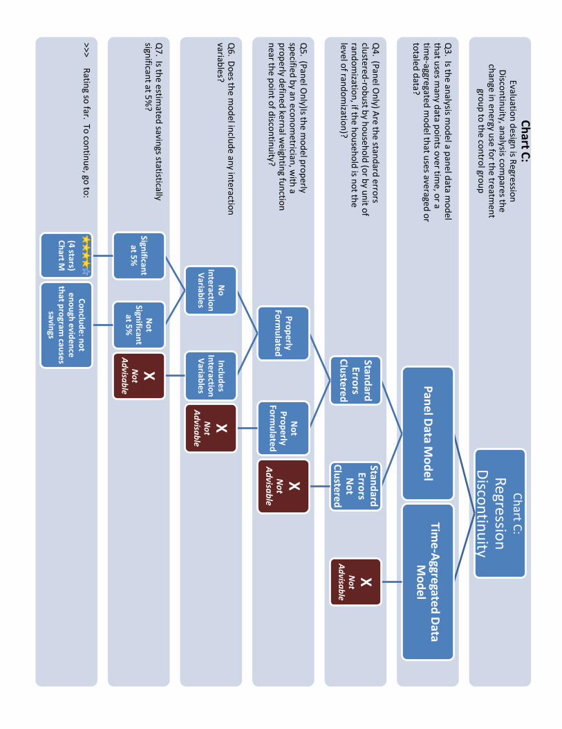
>>> R
ating so
far. To co
ntin
ue, go
to:
Q7
. Is the estim
ated savin
gs statistically sign
ificant at 5
%?
Q6
. Do
es the m
od
el inclu
de an
y interactio
n
variables?
Q5
. (Pan
el On
ly)Is the m
od
el pro
perly
specified
by an
econ
om
etrician, w
ith a
pro
perly d
efined
kernal w
eightin
g fun
ction
n
ear the p
oin
t of d
iscon
tinu
ity?
Q4
. (Pan
el On
ly) Are th
e stand
ard erro
rs clu
stered-ro
bu
st by h
ou
seho
ld (o
r by u
nit o
f ran
do
mizatio
n, if th
e ho
useh
old
is no
t the
level o
f rand
om
ization
)?
Q3
. Is the an
alysis mo
del a p
anel d
ata mo
del
that u
ses man
y data p
oin
ts ove
r time, o
r a tim
e-aggregated
mo
del th
at uses ave
raged o
r to
taled d
ata?
Ch
art C:
Evaluatio
n d
esign is R
egression
D
iscon
tinu
ity, analysis co
mp
ares the
chan
ge in en
ergy use fo
r the treatm
ent
grou
p to
the co
ntro
l grou
p
Ch
art C:
Regressio
n
Disco
ntin
uity
Pan
el D
ata Mo
de
l
Stand
ard
Errors
Clu
stered
Pro
perly
Form
ulated
No
In
teractio
n
Variab
les
Significan
t at 5
%
(4 stars)
Ch
art M
No
t Sign
ificant
at 5%
Co
nclu
de
: no
t e
no
ugh
evid
en
ce
that p
rogram
cause
s savin
gs
Inclu
de
s In
teractio
n
Variab
les
X
No
t A
dvisa
ble
No
t P
rop
erly Fo
rmu
lated
X
No
t A
dvisa
ble
Stand
ard
Errors
No
t C
lustered
X
No
t A
dvisa
ble
Time
-Aggre
gated
Data
Mo
de
l
X
No
t A
dvisa
ble

>>> R
ating so
far. To co
ntin
ue, go
to:
Q7
. Is the estim
ated savin
gs statistically sign
ificant at 5
%?
Q6
. Do
es the m
od
el inclu
de an
y interactio
n
variables?
Q5
. (Pan
el On
ly) Is the p
rop
ensity sco
re m
atchin
g algorith
m p
rop
erly specified
by an
eco
no
metrician
?
Q4
. (Pan
el On
ly) Are th
e stand
ard erro
rs clu
stered-ro
bu
st by h
ou
seho
ld (o
r by u
nit o
f ran
do
mizatio
n, if th
e ho
useh
old
is no
t the
level o
f rand
om
ization
)?
Q3
. Is the an
alysis mo
del a p
anel d
ata mo
del
that u
ses man
y data p
oin
ts ove
r time, o
r a tim
e-aggregated
mo
del th
at uses ave
raged o
r to
taled d
ata?
Ch
art D:
Evaluatio
n d
esign is P
rop
ensity Sco
re M
atchin
g; analysis co
mp
ares the ch
ange
in en
ergy use fo
r the treatm
ent gro
up
to
that o
f the co
ntro
l grou
p
Ch
art D:
Pro
pen
sity Score
Match
ing
Pan
el D
ata Mo
de
l
Stand
ard
Errors
Clu
stered
Pro
perly
Form
ulated
No
In
teractio
n
Variab
les
Significan
t at 5
%
(3 stars)
Ch
art M
No
t Sign
ificant
at 5%
Co
nclu
de
: no
t e
no
ugh
evid
en
ce
that p
rogram
cause
s savin
gs
Inclu
de
s In
teractio
n
Variab
les
X
No
t A
dvisa
ble
No
t P
rop
erly Fo
rmu
lated
X
No
t A
dvisa
ble
Stand
ard
Errors
No
t C
lustered
X
No
t A
dvisa
ble
Time
-Aggre
gated
Data
Mo
de
l
con
tinu
e
con
tinu
e
No
In
teractio
n
Variab
les
Significan
t at 5
%
(3 stars)
Ch
art M
No
t Sign
ificant
at 5%
Co
nclu
de
: no
t en
ou
gh
evid
en
ce w
ith th
is mo
de
l th
at pro
gram cau
ses
savings; su
ggest u
sing
pan
el d
ata mo
de
l Inclu
de
s In
teractio
n
Variab
les
X
No
t A
dvisa
ble

>>> Ratin
g:
Q1
0. W
ere the p
oten
tial-do
ub
le cou
nted
savings
accou
nted
for?
Q9
. Did
an in
dep
end
ent, th
ird-p
arty evaluato
r tran
sparen
tly defin
e and
imp
lemen
t:
•P
rogram
evaluatio
n
•A
ssignm
ent o
f ho
useh
old
s to co
ntro
l or treatm
ent
grou
ps
•D
ata selection
and
cleanin
g, inclu
din
g treatmen
t of
missin
g values, o
utliers, an
d acco
un
t closu
res, and
n
orm
alization
of b
illing cycle d
ays?
Q8
. Were d
ata from
ho
useh
old
s that o
pted
-ou
t in
clud
ed in
the an
alysis, and
was an
equ
valency
check p
erform
ed?
Ch
art M
Ch
art M
Op
t-ou
ts Inclu
ded
in
An
alysis, Eq
uivale
ncy C
heck
Pe
rform
ed
Third
Party
Imp
lem
en
ts All
Elem
en
ts
Do
ub
le-co
un
ted
savin
gs we
re
rigoro
usly
estimated
for all
pro
grams
Keep
All P
revio
us
Stars
Do
ub
le-co
un
ted
savin
gs estim
ated
on
ly for p
rogram
s th
at track e
fficien
cy m
easu
res
Sub
tract On
e Star fro
m P
revio
us
Score
Do
ub
le-co
un
ted
savin
gs we
re n
ot
estimated
X
No
t Ad
visab
le
Third
Party D
id
No
t Imp
lem
en
t A
ll Eleme
nts
X
No
t Ad
visab
le
Op
t-ou
ts Exclud
ed
in A
nalysis an
d/o
r Eq
uivalen
cy Ch
eck N
ot P
erfo
rme
d
X
No
t Ad
visab
le

May 2012 www.seeaction.energy.gov 52
Appendix B: Examples of Evaluations of Behavior-Based Efficiency Programs
This appendix reviews four behavior-based energy efficiency programs that provide real-world examples of the various design and analysis methodologies discussed in this report. These examples represent a range of various behavior program and evaluation types that can be used to target individual households, including feedback programs (e.g., home energy reports and in-home displays), energy goal-setting challenges, and other types of information treatments (e.g., energy saving tips sent in the mail).
To develop our set of four example programs, we identified 111 behavior-based efficiency programs implemented by utility and third-party program administrators through several sources. First, through generous assistance from the Consortium for Energy Efficiency (CEE), we received the CEE 2011 Behavior Program Summary, which provided information on 101 energy efficiency programs that were completed or are in progress. We then augmented that information by identifying 10 additional programs through several other sources:
The International Energy Program Evaluation Conference (IEPEC)
Behavior Energy and Climate Change (BECC) conference papers and poster sessions
American Council for an Energy-Efficient Economy (ACEEE) conference proceedings
Bonneville Power Administration’s “Residential Sector Research Findings for Behavior-Based Energy Efficiency”
Utility, third-party administrator, evaluation, and program implementation representatives.
We then screened for programs that met our study scope criteria, including:
Residential behavior-based programs, directed to the household level, that are not rate-based
At least one pilot year completed
A completed, publicly-available evaluation
Impact of interest on energy savings.
Twenty-six of the 111 programs met the above criteria and also incorporated RCT evaluation design. Among these 26 programs, 18 were Opower home energy report pilots (we also included two of these home energy report programs from different geographic regions to maximize the diversity of example programs).
We reviewed available program evaluations and selected four programs with evaluations that used rigorous EM&V approaches that garnered at least four stars in most of our rating categories:
Puget Sound Energy’s Home Energy Reports Program
Connexus Energy Home Energy Reports Program
Energy Center of Wisconsin PowerCost™ Monitor Study
Citizens Utility Board (CUB) Energy Saver Program.
The program examples are organized as follows.
Program summary
Description of how the program approached each of the various evaluation design and analysis methodologies
A summary table that includes our assessment of each study’s star ranking in each evaluation design and analysis and methodology category. Note that these summary tables do not provide an overall assessment of internal validity for any given study. Rather, they assess the relative strength of each component using the star system. To generate an overall assessment, one can apply the Checklist in Appendix A to each of these case studies.

May 2012 www.seeaction.energy.gov 53
Puget Sound Energy’s Home Energy Reports Program
Program Summary
In 2008, Puget Sound Energy (PSE), an electric and natural gas utility in Washington, implemented its first home energy reports (HERs) program, designed to encourage energy conservation behavior at the household level through normative messaging. Administered by Opower,
100 the PSE pilot provided HERs to nearly 40,000
households. The reports provide information about a household’s energy use to the occupants and compare the household’s energy usage to that of neighboring homes, essentially applying benchmarking and peer pressure to influence behavior to reduce energy usage in the home.
KEMA, a consulting firm that evaluates efficiency programs, conducted an evaluation of the first 20 months of the program (November 2008–June 2010). The report was published in October 2010.
101 KEMA’s evaluation reported
electric and gas savings for HER program participants using an RCT design and found that savings increased slightly over time. Average savings were estimated for three different time periods (see Table A-1).
Table A-1. Estimates of Savings for PSE’s Home Energy Reports Program
First 12 Months (11/08–10/09)
All 20 Months (11/08–6/10, annualized)
Last 12 Months (7/09–6/10)
Electric Savings 183.2 kWh 1.65% 204.5 kWh 1.84% 225.4 kWh 2.03%
Gas Savings 10.7 Therms 1.11% 12.1 Therms 1.26% 13.4 Therms 1.40%
Evaluation Design and Length of Study
The program used an RCT with opt-out recruitment. From all the households in PSE’s combined gas and electric service territory, the program implementer selected a group of 83,800 single-family homes that met certain criteria for the experimental design. Screening criteria included: King County household, dual fuel, single family residence, more than 80 MBtus
102 annual energy usage (the top 85%–88% of energy users), no solar PV system,
adequate utility billing information, and at least 100 similar sized homes within a 2 mile radius. 39,755 homes were then randomly assigned to receive the HER treatment with the remaining 44,045 homes serving as the control group receiving no HER. In the treatment group, 9,949 (25%) received HERS on a quarterly basis and 29,806 (75%) received monthly reports.
The 20-month evaluation relied on monthly billing data from both the treatment and control groups for the 15-month pretreatment period (July 2007–October 2008) and the 20-month program period (November 2008–June 2010).
Estimation Method
The KEMA evaluation employed a time-aggregated, difference-in-differences analysis model103
resulting in unbiased estimates of energy savings that were statistically significant at 1%.
104
100 Opower is a company contracted by energy efficiency program administrators to provide households with personalized information about their energy use via paper or an online portal. For pilot programs, the provided information typically includes a comparison to the energy use of nearby neighbors with similar-sized homes.
101 Kema 2010. Puget Sound Energy’s Home Energy Reports Program: 20 Month Impact Evaluation.
102 For ease of screening purposes, the program combined gas and electric usage, converting it into British Thermal Units (Btus).
103 The difference-in-differences approach compares the difference in average energy consumption between the pre- and post-treatment periods for both the treatment group and the control group to test the hypothesis that the treatment group will reduce its energy consumption. For the control group, the difference in energy usage between the pre- and post-treatment periods provides a robust estimate of any non-treatment related changes in energy consumption seen in the post-treatment period. The pooled regression approach models household monthly consumption as a combination of a household-specific base load, average heating and cooling trends, and monthly time-series effect, in order to replicate the difference-of-differences approach via a regression framework.

May 2012 www.seeaction.energy.gov 54
Table A-2. Summary of Design and Analysis Approaches for PSE’s Home Energy Reports Program
Approach and Ranking Rationale Star Ranking
Evaluation Design RCT, opt-out recruitment 5
Length of Study and Baseline Period
15 months pre-treatment data; 20 months treatment data 5
Avoiding Potential Conflicts of Interest
Program vendor conducted recruitment and group assignment; third-party evaluator conducted analysis
3
Analysis Models Difference-in-differences 4
Cluster-robust Standard Errors
Data were time aggregated; cluster-robust standard errors not needed
5
Standard Errors and Statistical Sign
Significant at the 1% level 5
Excluding Data from Households that Opt Out or Drop Out
Opt-out households were included in the data. Drop-outs (that closed accounts) were excluded.
5
Accounting for Potential Double Counting of Savings
The magnitude of double-counted savings was estimated, and at least 50% were allocated to the HER program for cost-effectiveness purposes.
5
External Validity The program did not attempt to extrapolate to different populations or future years.
5
Accounting for Double Counting of Savings
The evaluation included an examination of tracking data from other PSE energy efficiency programs. The HER includes energy saving tips and encourages participating households to both change habitual behaviors and take advantage of other PSE programs (e.g., appliance rebates), so the evaluation noted the potential for double counting savings if the HER drives participation in other programs that could be tracked to households in the treatment and control groups. However, the RCT design allowed evaluators to examine whether there appeared to be any systemic increase in participation in other programs among the treatment group relative to the control group.
Participation information for the PSE rebate program was gathered for all households in both the participant and control groups of the HER pilot. Rebate information from January 2007 to June 2010 was examined. Incorporating that information, KEMA used two different methodologies to estimate the amount of detected savings from the HER program that could potentially be double counted: a time of participation method and a load shape-allocated method. Preliminary examination of the data showed minimal evidence that the HERs increased participation in other programs among the treatment households.
Internal and External Validity
The estimates were not extrapolated to other populations or future years.
Connexus Energy Home Energy Report Program
Program Summary
In March 2009, Connexus Energy, a utility in Minnesota, implemented a new Home Energy Reports (HERs) pilot program with nearly 40,000 households in its territory. The reports, delivered via mail, provided information
104 Kema also employed a pooled methodology that examined the effect of the program during different types of weather; however, since that model includes interaction variables, it should not be used to calculate the program impact estimates. The results of the difference-in-difference method appear in the last two columns of Table C-1 of Appendix C of KEMA’s evaluation.

May 2012 www.seeaction.energy.gov 55
directly to households about their energy use and compared the household’s average energy usage over the prior 12 months to that of an aggregate of similarly-sized neighboring homes, employing benchmarking and peer pressure to influence behavior. This early incarnation of Opower’s
105 HER programs labeled comparatively low- and
moderate-consumption households as “great” and “good” respectively, with accompanying smiley-face emoticons. The reports also included suggested energy conservation actions that varied amongst households according to energy use levels and demographics.
Power Systems Engineering was hired as an independent third-party evaluator to validate methods and estimates of energy savings attributed to the program in the first year. They found similar estimated savings results using three different analysis methods: the true impact test (or difference-in-differences), ordinary least squares econometric model, and a fixed effects econometric model (see Table A-3).
Table A-3. Estimated Per-Customer Savings for Connexus Energy’s Home Energy Reports Program
Estimated annual kWh savings per customer relative to baseline
Estimated annual % reduction relative to
baseline Daily Annual
True Impact Test 0.621 227 2.05%
OLS Model 0.622 227 2.05%
Fixed Effects Model 0.637 232 2.10%
Average: 0.626 229 2.07%
Source: Power Systems Engineering, Inc. (2010)
Evaluation Design and Length of Study
The pilot was designed as an RCT with opt-out recruitment. Opower, the contracted program administrator, first identified 78,492 households that met screening criteria including: one active electric account per household; account history dating to January 2007; and at least 50 nearby households with similar-sized homes that use the same heating fuel. From the eligible households, 39,217 were randomly assigned to receive the HER treatment and 39,275 were assigned to the control group and received no HERs. Within the treatment group, subgroups were randomly assigned to receive HERs on a quarterly or monthly basis.
The Power Systems Engineering evaluation relied on monthly billing data from both the treatment group and control group for the two-year pretreatment period (January 2007–February 2009) and 12 month first-year pilot period (March 2009–January 2010). It does not provide information about treatment of data from opt-out customers.
An analysis by Hunt Allcott (2011) examined 13 months of pre-treatment billing data (January 2008–February 2009) and 20 months of treatment billing data (March 2009–November 2010). Alcott notes that 247 treatment households (0.6% of treatment households) opted out, but their billing data was retained in the analysis. Also during that period, about 1.25% of both the treatment and control group households closed their accounts. However, Allcott found no statistically significant difference between the two groups that closed their accounts, so those records were not included in the analysis.
Estimation Methods
Power Systems Engineering examined the sample selection, program design and data outputs, employing three analysis methods (the true impact test or difference-of-differences, an ordinary least squares (OLS) econometric
105 Opower is a company contracted by energy efficiency program administrators to provide households with personalized information about their energy use via paper or an online portal. For pilot programs, the provided information typically includes a comparison to the energy use of nearby neighbors with similar-sized homes.

May 2012 www.seeaction.energy.gov 56
model and a fixed effects econometric model) to estimate energy savings, which all resulted in similar savings estimates (2.05%–2.10%). The report indicated that estimates of energy savings using the OLS and fixed effects models were statistically significant at a 99% confidence level but it did not indicate whether the analysis included cluster-robust standard errors.
Allcott used a panel data model with household fixed effects, and used standard errors clustered at the household level. The model also included control variables in the form of 12 month-of-year specific dummy variables (i.e., one variable indicating whether or not the month was January, one indicating whether or not the month was February, etc.). The analysis found an average treatment effect (estimated savings) in the population of eligible households to be 1.9% below the pre-treatment baseline. The treatment effect was found to be larger for households with higher energy consumption and for those that received monthly reports as opposed to quarterly reports.
Accounting for Double Counting of Savings
Neither the Power Systems Engineering study nor Allcott explicitly discuss methods for estimating the potential double counting of savings. However, Allcott reports that customer surveys conducted as part of the pilot indicated that the bulk of behavioral changes caused by the Opower program were behaviors such as turning off lights and other actions that consumers already knew could save them energy. Further analysis of survey data might be able to estimate the impact of other Connexus residential programs on energy savings for these
households during the pilot period.
Internal and External Validity
Assuming the data are valid and the calculations are correct, the estimates of 1.9% average savings from the treatment as reported by Allcott and 2.07% as reported by Power Systems Engineering appear to be internally valid. The program administrator did not extrapolate estimated savings to other populations or future years, as savings estimates cannot be assumed for households within the Connexus territory that did not meet the screening criteria, or for households outside the Connexus territory. The estimates are also not valid for future years or new populations.
Summary of Design and Analysis Approaches
See Table A-4 for a summary of design and analysis approaches and the star ranking for each.

May 2012 www.seeaction.energy.gov 57
Table A-4. Summary of Design and Analysis Approaches for Connexus Energy Home Energy Report Program
Approach and Ranking Rationale Star Ranking
Evaluation Design RCT, opt-out recruitment 5
Length of Study and Baseline Period
Two years pre-treatment data; 20 months treatment data 5
Avoiding Potential Conflicts of Interest
Program vendor conducted recruitment and group assignment; third-party evaluator conducted analysis
3
Analysis Models Analysis models included difference-in-differences and panel data model.
5
Cluster-Robust Standard Errors
Panel data model used standard errors clustered at the household level.
5
Standard Errors and Statistical Sign
Significant at the 1% level 5
Excluding Data from Households that Opt Out or Drop Out
Alcott (2011) included opt-out households in the data. Drop-outs were tested and found to be statistically identical between treatment and control, so were excluded.
5
Accounting for Potential Double Counting of Savings
Analyses did not address potential double counting of savings.
0
External Validity The program did not attempt to extrapolate to different populations or future years.
5
Energy Center of Wisconsin PowerCost Monitor Program
Program Summary
In 2008, The Energy Center of Wisconsin (The Energy Center) implemented a study for Focus on Energy, Wisconsin’s third-party energy efficiency program administrator, to test the effectiveness of providing feedback to households via the PowerCost Monitor in-home energy display (IHD).
106 Program participants were drawn from
customers of five Wisconsin investor-owned electric utility service territories.107
Treatment households received a monitor and periodic season-appropriate tip sheets with energy saving ideas. Control households received neither a monitor nor tip sheets. Prior to the study, Focus on Energy determined that the pilot would need to obtain at least 2% savings to justify the development of a full-scale PowerCost Monitor program. The pilot estimated median savings of 1.4% for all participants who successfully installed the PowerCost monitor.
Evaluation Design and Length of Study
The pilot was designed as an RCT from a group of households that met certain criteria, including a willingness to participate in program surveys; thus, we consider this an opt-in program. The Energy Center selected participants using a random-digit-dialing system to ensure a representative sample of the general residential customer base of the participating utilities. They were then screened through telephone surveys conducted by an independent contractor, which produced an initial participant group of 735 households.
108 The screening criteria included:
owner-occupied single-family residence in current location for more than one year; primary heat source was not
106 The PowerCost Monitor™ is manufactured by Blue Line Innovations, Inc., and consists of a display device placed in the home that is connected to a battery-powered radio signal device attached to the customer’s electric meter. The display device provides information about the customer’s real-time and cumulative electricity use.
107 Alliant Energy, Madison Gas & Electric, We Energies, Wisconsin Public Service, and Xcel Energy.
108 The Blackstone Group, a subcontractor, implemented the telephone survey using a commercially available listed sample of Wisconsin households.

May 2012 www.seeaction.energy.gov 58
electricity; willingness to pay $25 for the PowerCost Monitor109
; written permission to access two years of utility billing data; and agreement to respond to two surveys during the pilot. Participants that met the criteria were then randomly assigned to treatment households (which received the devices as well as energy saving tip sheets) and control households (which did not receive devices or tip sheets). The Energy Center analysis examined two years of pre-pilot utility data and one year of utility data from the first year of the program.
To obtain written permission for accessing the billing data, release forms were sent to the 735 potential participants who met the other screening criteria. Release forms were sent to the treatment and control groups (with the only difference being the return address). Of the eligible participants, 462 (62%) returned signed forms; ultimately, the initial group assignments comprised 287 treatment households and 166 control households. Because the treatment group was much more likely to provide data than the control group, the estimated savings may have a large selection bias. In other words, basically a fraction of the control group has missing data resulting in a potentially biased savings estimate.
Estimation Methods
In its 2010 evaluation of the program, The Energy Center used a non-parametric bootstrap simulation110
model to estimate confidence intervals for energy savings. The evaluation initially analyzed electricity usage of 307 different accounts: 212 in the treatment group and 95 in the control group. The treatment group of 212 was further segmented according to the status of the devices at the end of the study: still functional (85 households); no longer functional (68 households); and never installed, unknown, or withdrawn (59 households). The primary billing analysis focused on the 153 households where the device was known to be installed and working, and the 95 control group households. The evaluation design did not provide any disaggregation of the effects of the monitor and the tip sheets.
The analysis included tests for various sub-groups of the treatment group against the control group: (1) treatment households that successfully installed the PowerCost Monitor; (2) households that consulted the monitor at least occasionally and for whom the device was functional when the end-of-study survey was conducted; (3) treatment households that consulted the monitor at least occasionally, and as often mid-study as they did at the beginning of the study; 4) treatment households that thought the monitor was useful in saving electricity.
The Energy Center reported that its overall findings of 1.4% estimated median savings were not statistically significant. However, in analysis of sub-groups, the treatment effect was found to be larger for households with higher pre-treatment energy consumption and for treatment households that said they consulted the monitor more frequently or that the monitor was helpful in reducing energy consumption.
111 Note that the savings
estimate is potentially biased because the treatment group seems to be different than the control group, based on the provision of data.
Accounting for Double Counting of Savings
Not indicated in evaluation.
Internal and External Validity
The program did not attempt to extrapolate to different populations or future years.
Challenges
109 Treatment households received the monitors at no cost; during the screening process, they were not told they would receive one. However, in order to participate in either the treatment or control group, participants needed to indicate a willingness to pay for the device.
110 Similar to a variation of a difference-in-differences analysis.
111 Excluding customers in the lowest quartile of annual electricity use increased the median savings of treatment households to 3.4% as compared to the control group. One of the survey questions asked whether the monitor was helpful in reducing electricity consumption.

May 2012 www.seeaction.energy.gov 59
This study shed light on several issues related to IHD-type programs. 17% of participants who received the monitor did not install it; from the group that installed the device, half of the households reported they could not get it to work.
112 In addition, only a subset of treatment households completed the mid-program and end-of-program
surveys, further reducing the number of participants that provided full information needed for the analysis. These issues resulted in a final participant group size much smaller than was initially recruited; the small numbers may have reduced the statistical significance of any treatment impacts. In addition, many households took significant time and technical assistance to get the devices installed and working, causing unexpected delays in the start of the program treatment.
Table A-5. Summary of Design and Analysis Approaches for Energy Center of Wisconsin PowerCost Monitor Program
Approach and Ranking Rationale Star Ranking
Evaluation Design RCT, opt-out recruitment with 153 in the treatment group and 95 in the control group
5
Length of Study and Baseline Period
Collection of pre-treatment billing data creates the potential for selection bias
0
Avoiding Potential Conflicts of Interest
Independent third-party impact analysis; independent subcontractor conducted recruitment and assignment of treatment and control groups and provided billing data, customer demographics, and weather data
5
Analysis Models Variation on difference-in-differences 5
Cluster-Robust Standard Errors
Not applicable N/A
Standard Errors and Statistical Sign
1.4% savings at 90% confidence interval N/A
Excluding Data from Households that Opt Out or Drop Out
Analysis excluded households that did not install devices, households that did not use the devices or get them working, and households that did not respond to the two surveys.
0
Accounting for Potential Double Counting of Savings
Not indicated 0
External Validity The program did not attempt to extrapolate to different populations or future years.
5
112 Some of the malfunction was attributed to end of battery life and improper resetting of the monitor when batteries were replaced.

May 2012 www.seeaction.energy.gov 60
ComEd CUB Energy Saver Program—Online Program with Rewards for Saving Energy
Program Summary
In July 2010, Efficiency 2.0,113
an energy efficiency program vendor, and the Citizens Utility Board (CUB)114
of Illinois formed a partnership to implement the CUB Energy Saver pilot program for Commonwealth Edison (ComEd), the largest electric utility in Illinois, which serves the Chicago and Northern Illinois area.
The CUB Energy Saver program encourages customers to reduce energy usage by providing feedback on energy usage and recommendations for energy saving behaviors and measures via mailers or online engagement, and by offering rewards
115 for achieving energy saving goals.
116 The CUB Energy Saver pilot consisted of two different
treatments: a mailer-only information campaign with opt-out recruitment (participants did not choose to receive the mailers) and an opt-in online program in which participants actively chose to participate. This summary focuses on the online portion of the program.
Online participants were primarily recruited through direct-mail solicitation to ComEd customers in addition to many community marketing activities such as media coverage and competitions with local towns. Households received 100 reward points (redeemable for such rewards as a $10 gift card or 20% off at online stores) for opting in and completing the sign-up process. Successful sign-up consists of completing three steps: (1) providing basic contact info; (2) providing utility account information to allow access to past and future billing info; and (3) reviewing and choosing from a menu of energy savings plans corresponding to roughly 5%, 10%, and 15% annual electricity savings (labeled as “no cost,” “low cost,” and “home investment” plans). Each plan offers a list of energy savings recommendations—and is customized to some extent based on rough estimates derived from a statistical model of household energy use and appliance saturation. Users can add additional energy saving actions from a long list, and can customize each action—effectively committing to a goal (e.g., fill in how many light bulbs will be replaced by CFLs and the number of hours they will be used per day). During the program, the user receives detailed information including dollars saved as a result of implementing particular actions and the amount of carbon emissions reduced and kilowatt-hours saved (Harding and Hsiaw 2011).
Customers are then rewarded two points (up to 250 points per billing period) for every kilowatt-hour saved relative to the previous year’s usage (adjusted for weather in a process outside the customer’s control). Points can then be redeemed for coupons on the website. The customer does not lose points for not saving energy, and there is a cap on the maximum number of points that can be awarded. Points are only roughly correlated to actual energy savings. Unlike home energy reports programs, the CUB program does not provide feedback that compares the participants’ energy use to that of other households.
Evaluation Design and Length of Study
The CUB Energy Saver program utilized a quasi-experimental design. Households opted in to the online program, and were not randomized into a control or treatment group. As such, they are likely to have some different characteristics from households that did not opt to participate, and therefore program impact estimates based on comparing opt-in households to those that did not opt in may result in biased savings estimates (i.e., the households that did not opt in are not a valid control group for those that did opt in).
113 Efficiency 2.0 is a nationwide vendor of energy efficiency behavior-based programs that provides mail-based, household-specific energy reports and recommendations and online customer engagement strategies.
114 CUB is a nonprofit, nonpartisan ratepayer advocacy organization established in 1983 by the Illinois General Assembly.
115 Rewards are provided in the form of points, which customers can redeem for merchandise with partner companies.
116 In Efficiency 2.0 online programs, participants receive 100 points (good for $10 gift cards or a 20% discount from participating online retailers) simply for signing up and linking their utility bills to the program, allowing Efficiency 2.0 access to utility billing data for program analysis. For every kilowatt-hour participants save in their monthly bill over baseline, they are awarded two points (up to 250 points per billing period). Individual savings are calculated by comparing projected baseline usage to actual usage for a given billing period.

May 2012 www.seeaction.energy.gov 61
In order to address this issue of bias, Harding’s 2011 evaluation of the program (Harding and McNamara 2011, also see Harding and Hsiaw 2011) used a variation in adoption approach with rigorous testing of assumptions (see boxed text).
Efficiency 2.0 provided raw electricity usage and household characteristic data to Matthew Harding of Stanford University, who conducted an analysis of the program over a 12-month period (July 2010–July 2011). The electricity usage and household information was accessed through a partnership with CUB and ComEd.
Estimation Methods
The evaluation used a used a variation in adoption approach with a panel data model analysis method with correctly calculated standard errors, using rigorous robustness tests. It yielded a savings estimate of 3%, significant at the 1% level.
Accounting for Double Counting of Savings
The CUB Energy Saver program conducted a survey117
to identify the actions participants were taking to save energy,
118 and to report on the number of rebates or direct incentives they received from other programs both
before and after they joined the program. Seventy-nine percent of survey respondents reported they did not receive a rebate or other incentive from ComEd before or during program participation. More than 6% of respondents reported receiving an incentive after the program, but not before, and nearly 9% reported the opposite. An additional 6% reported receiving incentives both before and after participating in CUB Energy Saver. A detailed analysis of double counting of savings is planned.
Internal and External Validity
The program did not attempt to extrapolate to different populations or future years.
Summary of Design and Analysis Approaches
See Table A-6 for a summary of design and analysis approaches and the star ranking for each.
117 The evaluation does not indicate what percentage of program participants completed the survey. The answers were open-ended and respondents were given a $5 Amazon.com gift card for taking the survey.
118 83% of respondents reported making behavioral changes (e.g., turning off lights, raising the air conditioner temperature setting) and 25% reported making equipment changes; 80% of the group that made equipment changes made behavior changes as well.

May 2012 www.seeaction.energy.gov 62
Table A-6. Summary of Design and Analysis Approaches for ComEd CUB Energy Saver Program
Approach and Ranking Rationale Star Ranking
Evaluation Design Quasi-experimental design with opt-in recruitment: a variation in adoption technique with rigorous robustness tests. Not a full RCT.
3.5
Length of Study and Baseline Period
One year pre-treatment data; one year of treatment data 5
Avoiding Potential Conflicts of Interest
Program vendor conducted recruitment and group assignment. One evaluation done by program vendor, Harding and McNamara (2011); one done by paid academics, Harding and Hsiaw (2011). Independent third-party evaluator scheduled to complete formal evaluation.
1; 3 planned
Analysis Models Panel data model 5
Cluster-Robust Standard Errors
Yes 5
Statistical Significance Significant at 1% 5
Excluding Data from Households that Opt Out or Drop Out
Accurately excluded households 5
Accounting for Potential Double Counting of Savings
Program surveyed participants about participation in other ComEd incentive and rebate programs. Analysis of double counting is planned.
(Planned)
External Validity The analysis did not attempt to extrapolate to different populations or future years.
5
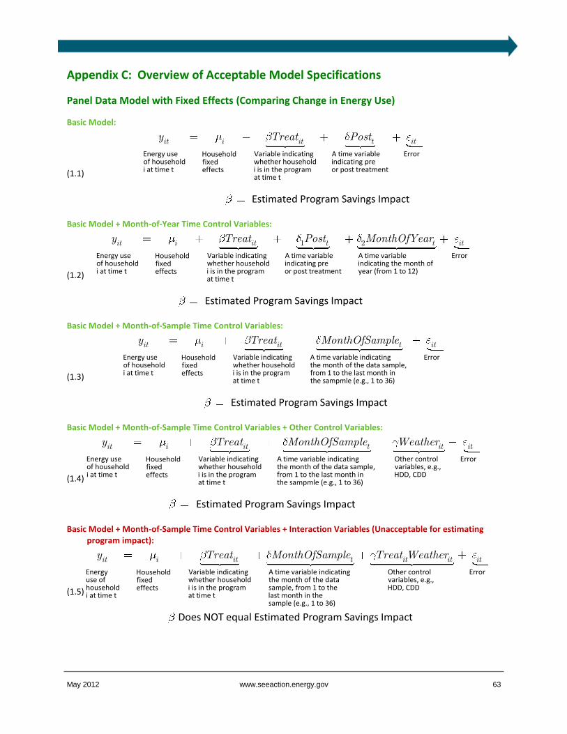
May 2012 www.seeaction.energy.gov 63
Appendix C: Overview of Acceptable Model Specifications
Panel Data Model with Fixed Effects (Comparing Change in Energy Use)
Basic Model:
(1.1)
it i it ty PostTreat
Energy use Variable indicating A time variable Household of household whether household indicating pre fixed i at time t i is in the program or post treatmenteffects
at time t
it
Error
Estimated Program Savings Impact
Basic Model + Month-of-Year Time Control Variables:
(1.2)
1it i it ty PTrea ost t
Energy use Variable indicating A time variable Household of household whether household indicating pre fixed i at time t i is in the program or post treatmenteffects
at time t
2 t itMonthOfYear
A time variable Errorindicating the month of year (from 1 to 12)
Estimated Program Savings Impact
Basic Model + Month-of-Sample Time Control Variables:
(1.3)
it i it tTreay MonthOfSamplt e
Energy use Variable indicating A time variable indicating Household of household whether household the month of fixed i at time t i is in the programeffects
at time t
it
Errorthe data sample,
from 1 to the last month in the sampmle (e.g., 1 to 36)
Estimated Program Savings Impact
Basic Model + Month-of-Sample Time Control Variables + Other Control Variables:
(1.4)
it i it tTreay MonthOfSamplt e
Energy use Variable indicating A time variable indicating Household of household whether household the month of fixed i at time t i is in the programeffects
at time t
it itWeather
Other control variables, e.g., HDD, CDD
Errorthe data sample,
from 1 to the last month in the sampmle (e.g., 1 to 36)
Estimated Program Savings Impact
Basic Model + Month-of-Sample Time Control Variables + Interaction Variables (Unacceptable for estimating program impact):
(1.5)
it i it ty MonthOfSamplTreat e
Energy Variable indicating A time variable indicating Household use of whether household the month offixed household i is in the programeffectsi at time t at time t
it it itTreat Weather
Other control variables, e.g., HDD, C
Error the data
sample, from 1 to the last month in the sample (e.g., 1 to
DD
36)
Does NOT equal Estimated Program Savings Impact
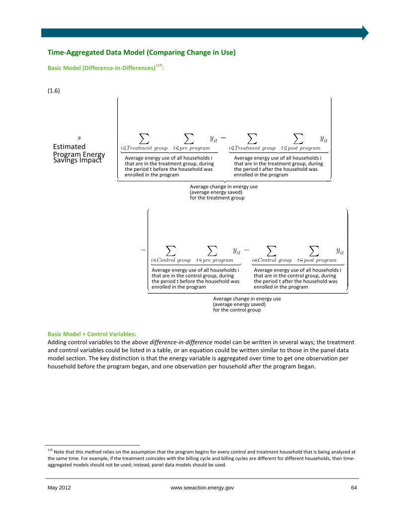
May 2012 www.seeaction.energy.gov 64
Time-Aggregated Data Model (Comparing Change in Use)
Basic Model (Difference-in-Differences)119
:
(1.6)
iti Treatment group t pre program
s y
Average energy use of all households i that are in the treatment group, duringthe period t before the household wasen
rolle
EstimatedProgram EnergySavings Impact
iti Treatment group t post program
y
Average energy use of all households i that are in the treatment group, duringthe period t after the household was
d in
the program enrolled in the program
Average change in energy use (average energy saved)for the treatment group
iti Control group t pre program
y
Average energy use of all households i that are in the control group, duringthe period t before the household wasen
r
olle
iti Control group t post program
y
Average energy use of all households i that are in the control group, duringthe period t after the household was
d in
the program en
rolled in the program
Average change in energy use (average energy saved)for the control group
Basic Model + Control Variables: Adding control variables to the above difference-in-difference model can be written in several ways; the treatment and control variables could be listed in a table, or an equation could be written similar to those in the panel data model section. The key distinction is that the energy variable is aggregated over time to get one observation per household before the program began, and one observation per household after the program began.
119 Note that this method relies on the assumption that the program begins for every control and treatment household that is being analyzed at the same time. For example, if the treatment coincides with the billing cycle and billing cycles are different for different households, then time-aggregated models should not be used; instead, panel data models should be used.

May 2012 www.seeaction.energy.gov 65
Panel Data Model without Fixed Effects (Comparing Use Rather Than Change in Use)
Basic Model:
(1.7) (
it i itTreaty
Energy use Variable indicating Errorof household whether householdi at time t i is in the program
is in the treatmentgroup) or is in the control group
Estimated Program Savings Impact
Basic Model + Month-of-Year Time Control Variables:
(1.8) (
2it i ty MonthOfYeaTreat r
Energy use Variable indicating A time variable of household whether household indicatii at time t i is in the program
is in the treatmentgroup) or is in the control group
it
Errorng the month of
year (from 1 to 12)
Estimated Program Savings Impact
Basic Model + Month-of-Sample Time Control Variables:
(1.9) (
it i ty MonthOfSampTrea let
Energy use Variable indicating A time variable indicatof household whether householdi at time t i is in the program
is in the treatmentgroup) or is in the control group
it
ing Errorthe month of the data sample, from 1 to the last month in the sampmle (e.g., 1 to 36)
Estimated Program Savings Impact
Basic Model + Month-of-Sample Time Control Variables + Other Control Variables:
(1.10) (
it i ty MonthOfSampTrea let
Energy use Variable indicating A time variable indicatof household whether householdi at time t i is in the program
is in the treatmentgroup) or is in the control group
it itWeather
ing Errorthe mont
Other control variables, e.h of the data s g., HDD, CDD
ample, from 1 to the last month in the sampmle (e.g., 1 to 36)
Estimated Program Savings Impact
Basic Model + Month-of-Sample Time Control Variables + Interaction Variables (Unacceptable for estimating program impact):
(1.11) (
it i iy MTr onthOfSameat
Energy Variable indicatingHousehold use of whether householdfixed household i is in the programeffectsi at time t is in the treatment
group) or is in the control group
t it itTreat Weatheple r
A time variable indicating the month of the data sample, from 1 to the last month in the sample (
Other control variables, e.g., HDD, CDD
e.g., 1 to 36)
it
Error
Does NOT equal Estimated Program Savings Impact

May 2012 www.seeaction.energy.gov 66
Time-Aggregated Data Model (Comparing Use)
Basic Model (Difference-in-Averages):
(1.12) it
i Control group t post program
s y
Average energy use of all households i that are in the control group, duringthe period t after the househol
d wasenrolled in
EstimatedProgram EnergySavings Impact
iti Treatment group t post program
y
Average energy use of all households i that are in the treatment group, duringthe period t after the household was
the program e
nrolled in the program
Basic Model + Control Variables: Adding control variables to the above difference-in-averages model can be written in several ways; the treatment and control variables could be listed in a table, or an equation could be written similar to those in the panel data model section. The key distinction is that the energy variable is aggregated over time to get one observation per household after the program began.
Energy Variable: Natural Log or Not?
We recommend performing all analyses with the untransformed variable of energy use, rather than the transformed variable of the natural log of energy use (typically written ln(y)). Analyzing the data with an untransformed variable will yield an estimate of the effect of the program averaged over all households in kilowatt-hour terms, while analyzing the data with the log of energy will yield the effect of the program averaged over all households in percentage terms. Because higher energy use households may tend to save more energy as a result of the program, performing the analysis with the log of energy use may lead to a misleadingly small estimate of energy use. To see why, imagine that there are only two households: a high energy use household that saved 100 kWh out of 1,000 kWh, which was 10% of their usage, as a result of the program; and a low energy use household that saved 10 kWh out of 500 kWh, which was 2% with the program. The total amount of energy saved was 110 kWh out of 1,500 kWh. The effect of the program is to save 7.3% of total energy (110 / 1,500), but the effect of the program averaged over households in percentage terms is 6% ((2% + 10%) / 2).

May 2012 www.seeaction.energy.gov 67
Appendix D: Program Design Choices
This section discusses two program design choices: the enrollment method, either opt-in or opt-out; and the way that the households are screened in order to be eligible to participate at all. These choices affect the population for which the program impacts are valid (i.e., if the program is opt-in and restricted to high energy users, then the estimates of energy savings are only valid for the type of households that opt in to the program and are high energy users). However, they do not actually affect the level of bias and precision of the estimate of program impacts—as long as there are enough households overall and the correct evaluation methods and procedures are applied.
120
Opt-In versus Opt-Out
As described above, a randomized controlled trial (RCT) can be done with either an opt-out or an opt-in enrollment method, and either one will result in unbiased estimates of energy savings. One consideration is that in general, more households will remain in an opt-out program than will sign up for an opt-in program, and so an opt-out method will result in more program participants.
Another consideration is that the types of people that choose to opt in to a program may be very different, particularly in terms of their concern about energy use, than the types of people that would not choose to opt in to a program. Depending on how they are different, this could have different implications.
If the type of households that opt in are more likely to reduce their energy use even in the absence of the program (e.g., they have decided to do all that they can to lower their energy bills, and they came across the program and decided to enroll in it), then there are two implications: first, these people may not be the ones to target because they would reduce energy use in any case (although alternatively they may be excellent targets if the program can provide them with the information and means to implement their desire to reduce energy use/costs); and second, without a randomized control group, the estimate of energy savings from these households would seem as if the program was very effective when in fact the households would have reduced energy in any case (the savings estimates would be much higher than the true savings).
On the other hand, if the type of households that do not opt in would never be interested in saving energy regardless of whether they are enrolled in a program or not, then it is a waste of resources to include those that do not opt in to a program. Thus, having an opt-in program may be a good design feature because it segments the population in exactly the way that targets those that are most likely to benefit from a program.
A final consideration is applying savings estimates to populations outside the initial program population. If the initial program is opt-in, then estimates from the initial program are more likely to be applicable to new populations that are also the type of households that would opt in, but are likely not to be applicable to new opt-out populations. If the initial program is opt-out, then estimates from the initial program are more likely to be applicable to new opt-out populations.
Restriction or Screening of Initial Population
There are many reasons why a program may be screened or restricted to certain households. There are two major categories of restrictions: non-random restrictions, such as screening households based on location or level of energy consumption; and random restrictions, when a random sample of a larger population is taken in order to reduce the population size for cost or other reasons.
120 See previous footnote.

May 2012 www.seeaction.energy.gov 68
Non-Random Restrictions
Households in a program may have to go through a screening process before being considered for the program. Often this screening process restricts the study population to specific geographies (zip codes or service areas), specific demographics (low income, medical needs, elderly), specific customer characteristics (high energy users, dual fuel use, length of customer bill history), specific data requirements (one year of historical energy data available, census information is available, smart meter installed), and other restrictions.
One reason to restrict households in this way is that if the households in the program are more similar to each other, then there is lower variation in customer characteristics, which would result in a more precise estimate of energy savings and thus the ability use smaller control group populations. Another reason to restrict households is if there is prior knowledge about a segment of the population for which the program is particularly effective. In this case, it is more cost effective to target the program to those households.
On the other hand, any estimates of savings are only valid for the group of restricted households, and so more restrictions means that the program impacts are valid for a smaller subset of the population. For example, if the population is restricted to high energy use households, then the estimates of savings are not likely to be applicable to low or moderate energy use households.
It is important to keep in mind that when creating a control group, the control group must be taken from the same group of restricted households as the treatment group. Otherwise, the groups are different by construction and then differences between the energy savings of the two groups could be due to either the program or to the inherent differences in the groups.
Random Sample Restrictions
A population may also be restricted to certain households in a random way: if a population is too big, then a smaller population can be randomly sampled from the larger population. Note that this is different than random assignment into a control and treatment group: here, first the smaller population is randomly sampled from the larger population, and then the smaller population is divided into a control and treatment group. This could be combined with non-random restrictions, for example, first the population is restricted to only single family households, and then out of all single family households one in every 100 households is randomly chosen to be in the study population and is assigned to either the control group or the treatment group.
One benefit of restricting the population in this way is that savings estimates from the initial population are more likely to be valid for the larger population from which they were sampled.

This document was developed as a product of the State and Local Energy Efficiency Action Network (SEE Action), facilitated by the U.S. Department of Energy/U.S. Environmental Protection Agency. Content does not imply an endorsement by the individuals or organizations that are part of SEE Action working groups, or reflect the views, policies, or otherwise of the federal government.