evaluation and optimization of an industrial utility system

FACULDADE DE ENGENHARIA DA UNIVERSIDADE DO PORTO

Evaluation and Optimization of an Industrial

Utility System

João Alegre Queiroz

Doctoral Program in Refining, Petrochemical and Chemical Engineering

Academic supervisors: Fernando Martins (UP – FEUP - LEPABE)

Henrique Matos (UL - IST - CERENA)

Industrial coordinator: Vítor Rodrigues (Dow Portugal)

February 2016

Evaluation and Optimization of an Industrial

Utility System

João Alegre Queiroz

Doctoral Program in Refining, Petrochemical and Chemical Engineering

Work financially supported by

under the program Bolsas de Doutoramento em Empresas (SFRH/BDE/51013/2010).

February 2016

V

Resumo

Num contexto global, é fundamental reduzir a energia consumida com origem em combustíveis fósseis de

forma a minimizar o impacto ambiental da atividade humana. A contribuição da indústria para a energia

total consumida é bastante elevada (em 2013 correspondeu a 30% da energia total consumida

mundialmente de acordo com Agência Internacional de Energia), pelo que a redução do consumo

energético neste setor é bastante incentivada. Do ponto de vista da indústria, a redução de custos induzida

pela minimização do consumo energético representa outro fator de extrema relevância.

A diminuição das reservas de combustíveis fósseis e o aumento da concentração dos gases com efeito de

estufa motivam o desenvolvimento de um sistema sustentável que utilize menos combustíveis fósseis. De

forma a minimizar a sua utilização duas vias deverão ser exploradas:

Desenvolvimento e introdução de novas tecnologias de produção, armazenamento e utilização de

energia, que não se baseiem em combustíveis fósseis;

Medidas de conservação energética (intensificação) para utilização mais eficiente dos recursos

energéticos.

O estudo que foi desenvolvido e é aqui apresentado foca-se nesta última estratégia e visa a aplicação de

ferramentas e metodologias de otimização energética aplicáveis em ambiente industrial.

Numa instalação industrial de produção de produtos químicos é comum a utilização de vapor e água de

arrefecimento como meios de distribuição energética de e para o processo. O foco deste estudo é o

desenvolvimento de metodologias nos dois seguintes tópicos:

1. Avaliar o desempenho térmico e hidráulico dos sistemas de vapor e água de arrefecimento através

de modelos suportados em ferramentas informáticas;

2. Identificar fontes de desperdício e oportunidades de melhoria que visem a melhoria do

desempenho energético da unidade.

As ferramentas e metodologias desenvolvidas foram utilizadas para identificar oportunidades de melhoria

na fábrica da Dow Portugal, em Estarreja. Foi possível identificar oportunidades de melhoria que reduziriam

em cerca de 11% os custos energéticos operacionais, representado cerca de 1 M€ de poupança anual.

Estas modificações também permitiram reduzir o tempo em que a torre de arrefecimento é o ponto de

estrangulamento da fábrica, permitindo reduzir este período de 4.5% para 3% do tempo total de operação

da fábrica.

Palavras-chave: energia; sistema de água de arrefecimento; sistema de vapor; integração de processo;

tecnologia do estrangulamento térmico, método matricial

VII

Abstract

In a global context, it is fundamental to reduce the fossil-based energy consumption to minimize the

environmental impact of human activities. Industry’s contribution to the total energy consumption is very

high (in 2013 corresponded to 30% of the total energy consumption worldwide according to the International

Energy Agency [1]), and thus reduction of energy use is highly motivated in this sector. From the industry

viewpoint, cost savings represent another key driver for energy optimization.

The diminishing supplies of fossil fuels and increased greenhouse gas levels motivate research and

development towards a sustainable energy system with less use of fossil fuels. To decrease this use, two

main paths must be pursued:

• Development and introduction of new energy production techniques, not relying on fossil fuels;

• Energy conservation (intensification) measures to use energy more efficiently.

The study presented herein is focuses on the latter approach and aims for the application of energy

optimization tools and methodologies, applicable in an industrial context.

Within a chemical manufacturing plant, steam and cooling water are two major utilities in regard to energy

in- and output to/from the processes. The aim of this work is to contribute through the development of

methods in two subjects:

1. Evaluating thermal and hydraulic performance of steam and cooling water systems through

computer-based mathematical models;

2. Identifying waste sources and cost-effective retrofit improvements to the steam and cooling water

systems.

The developed tools and methodologies were applied in a practical example of Dow Portugal, in Estarreja,

to identify improvement opportunities. It was possible to identify possible modifications that could result in

a 11% operational cost reduction, representing around 1 M€/yr savings. These modifications would also

allow to reduce the time during which the cooling tower is the production bottleneck, allowing a reduction

of this period from 4.5% to 3% of the total operating time.

Keywords: Energy; cooling tower; cooling water system; steam system; process integration; stream

matching; pinch analysis; matrix method

IX

Acknowledgements

I am truly grateful to my academic supervisors: Prof. Fernando Martins (UP-FEUP) and Prof. Henrique

Matos (UL-IST) for all the support, guidance and advice that were fundamental to complete this

endeavour. Without their commitment and encouragement most of the achievements of this project would

have been compromised.

To my supervisor at Dow Portugal, Vitor Rodrigues, a word of deep gratitude for being key to the

development of the project and for teaching me so many things at the professional level as well as the

personal level. I will most certainly use much of his insights throughout my life.

I also acknowledge the Doctoral Program in Refining, Petrochemical and Chemical Engineering,

Faculdade de Engenharia da Universidade do Porto, Instituto Superior Técnico, Fundação para a Ciência

e a Tecnologia and Dow Portugal for making this project possible.

A big “Thank you!” is also owed to my parents, family and friends who supported me at all times and gave

me words of advice and wisdom throughout this journey.

Finally, I have no words to express my gratitude towards Raquel and Afonso, whose love and patience

was fundamental for the sanity of the author and without whom everything would be infinitely harder.

XI

Table of contents

1 Introduction ......................................................................................................................... 1

1.1 Motivation ..................................................................................................................................... 1

1.2 Scope ............................................................................................................................................ 1

1.3 Industrial context ........................................................................................................................... 2

1.3.1 Process description .............................................................................................................. 4

1.4 Thesis outline ................................................................................................................................ 5

2 Energy efficiency optimization overview .............................................................................. 7

2.1 Data extraction ............................................................................................................................ 10

2.2 Utility system analysis ................................................................................................................. 13

2.2.1 Cooling water system ......................................................................................................... 14

2.2.2 Steam system ..................................................................................................................... 16

2.3 Retrofit heat exchanger networks ............................................................................................... 18

2.3.1 Pinch analysis ..................................................................................................................... 20

2.3.2 Mathematical programming ................................................................................................ 28

2.3.3 Hybrid methods ................................................................................................................... 29

3 Utility system analysis ....................................................................................................... 30

3.1 Cooling water system ................................................................................................................. 30

3.1.1 Hydraulic model of cooling water network .......................................................................... 30

3.1.2 The cooling tower model ..................................................................................................... 34

3.1.3 Cooling system thermodynamic model ............................................................................... 50

3.1.4 Evaluation of the performance of the cooling water system ............................................... 56

3.2 Steam system analysis ............................................................................................................... 59

3.2.1 Steam generator ................................................................................................................. 59

3.2.2 Steam network .................................................................................................................... 69

XII

3.2.3 Steam system thermodynamic model ................................................................................ 71

3.2.4 Steam cost estimation ........................................................................................................ 79

4 Stream match methodology .............................................................................................. 81

4.1 Methodology framework ............................................................................................................. 82

4.2 Stream matching illustrated with Case Study 1 .......................................................................... 86

Step 1 - Determine process pinch temperature ................................................................................. 87

Step 2 - Split streams at the pinch according to pinch rules .............................................................. 89

Step 3 - Match streams above the pinch ........................................................................................... 90

Step 4 - Match streams below the pinch ............................................................................................ 98

Step 5 - Optimize temperature approach of heat exchangers at the pinch ..................................... 103

4.3 Case study 2 - Retrofit heat exchanger network (Industrial application) .................................. 105

4.4 Impact on cooling tower operation ............................................................................................ 122

4.5 Impact on the steam network ................................................................................................... 123

5 Conclusions and Recommendations ............................................................................... 126

5.1 General conclusions ................................................................................................................. 126

5.2 Recommendations for future work ............................................................................................ 127

6 References ..................................................................................................................... 128

Appendix ................................................................................................................................ 136

A1 (Air properties) ................................................................................................................................ 136

A2 (Stream matching) .......................................................................................................................... 140

A3 (Stream match tools)....................................................................................................................... 142

A3.3.1 Above pinch.xls .................................................................................................................... 142

A3.3.2 Bellow pinch.xls .................................................................................................................... 148

A3.3.3 Pinch Tool.xls ....................................................................................................................... 149

XIII

List of Figures

Figure 1.1 – Molecular structure of monomeric and polymeric MDI. ............................................................ 2

Figure 1.2 – Overview of the Estarreja chemical cluster [4]. ........................................................................ 3

Figure 1.3 – Process block diagram. ............................................................................................................ 4

Figure 1.4 – Main products and reaction steps involved in the MDI manufacturing process. ...................... 5

Figure 1.5 – Word cloud with the terms using in this thesis. ........................................................................ 5

Figure 1.6 – Thesis structure and summary of each chapter. ...................................................................... 6

Figure 2.1 – An effort to reduce external utilities’ quality and quantity is constantly pursued. ..................... 7

Figure 2.2 – Word cloud showing the prominence of the Keywords that appear more frequently in the

works returned by www.ScienceDirect.com with the search words “Process Integration” (August 2014). .. 8

Figure 2.3 – Methodology for the overall process energy evaluation and optimization. .............................. 9

Figure 2.4 – Sequential-Modular architecture diagram (Adapted from [17]). ............................................. 11

Figure 2.5 – Sequential modular approach (a) without recycle stream and (b) with recycle stream. ........ 12

Figure 2.6 – Trade-offs in heat exchanger network design (Adapted from Yee and Grossman [51]). ...... 19

Figure 2.7 – Temperature-Enthalpy profile of a countercurrent heat exchanger. ...................................... 23

Figure 2.8 – Two hot streams represented in the T-Q plot. ....................................................................... 24

Figure 2.9 – Stream 1 and 2 combined in one single composite curve. .................................................... 24

Figure 2.10 – Hot and cold composite curves in the same T-Q plot. ......................................................... 25

Figure 2.11 – Energy targets given by the combined composite curves.................................................... 25

Figure 2.12 – Composite curve shifting. ..................................................................................................... 26

Figure 2.13 – Construction of the grand composite curve.......................................................................... 26

Figure 2.14 – Grand Composite Curve used to determine utility targets in (a) a process with only two

utility levels and (b) a process with multiple utilities levels. ........................................................................ 27

Figure 2.15 – Hot and cold composite curves for: (a) a process with minimum energy requirements, (b) a

process where α amount of heat is transferred across the pinch and (c) a process with γ amount of

external cooling and β amount of external heating above and below the pinch, respectively. .................. 28

Figure 3.1 - Detail of the cooling water pumps and heat exchanger network in SiNET. .......................... 31

Figure 3.2 – The cooling water network in SiNET. ..................................................................................... 32

Figure 3.3 – Comparison between design and simulated flow of current network configuration. Relative

difference between design and improved network configuration is also presented. .................................. 33

XIV

Figure 3.4 – Representation of a cooling tower with N equilibrium stages. The air stream enters the

cooling tower at the bottom stage and leaves at the top stage; it is characterized by its dry bulb

temperature (Ta), flow (G) and relative humidity (RH). Water stream enters the cooling tower at the top

stage and leaves at the bottom stage; it is characterized by its temperature (Tw) and flow (L). ................ 36

Figure 3.5 – Algorithm for the evaluation of the model parameters. The inner circle of the algorithm is a

NLP problem whereas if the number of equilibrium stages is considered it is a MINLP problem. ............. 39

Figure 3.6 – Overall procedure flowchart showing the interaction between the process simulator (ASPEN

PLUS) and the minimization algorithm (implemented in Microsoft Excel), being this interaction mediated

by Aspen Simulation Workbook. The steps referred in this figure are described in detail in Section 2 of

this work. ..................................................................................................................................................... 42

Figure 3.7 – Objective function evolution for tower R-1 for training [■] and validation [□] sub-sets. .......... 45

Figure 3.8 – Objective function evolution for tower R-2 for training [■] and validation [□] sub-sets. .......... 46

Figure 3.9 – Objective function evolution for Dow’s tower for training [■] and validation [□] sub-sets. ...... 46

Figure 3.10 – Water outlet temperature model predictions vs. observed value for tower R-1: (a) Training

[◊] + validation [■] and (b) test [▲]. Assuming a constant Patm of 101.3 kPa. ............................................ 47

Figure 3.11 – Water outlet temperature model predictions vs. observed value for tower R-2: (a) Training

[◊] + validation [■] and (b) test [▲]. Assuming a constant Patm of 101.3 kPa. ............................................ 47

Figure 3.12 – Water outlet temperature model predictions vs. observed value for Dow’s tower: (a)

Training [◊] + validation [■] and (b) test [▲]. .............................................................................................. 48

Figure 3.13 – Air outlet temperature model predictions vs. observed value for training [◊], validation [■]

and test [▲] in: (a) Tower R-1 and (b) tower R-2. Assuming a constant Patm of 101.3 kPa. ...................... 48

Figure 3.14 – Block diagram of the cooling water system model. .............................................................. 51

Figure 3.15 – Detail of the cooling tower thermodynamic model implemented in ASPEN PLUS. ............. 53

Figure 3.16 – Detail of the cooling water network thermodynamic model implemented in ASPEN PLUS. 55

Figure 3.17 – ASPEN PLUS model of cooling water network integrated with cooling tower. .................... 55

Figure 3.18 – Cooling water supply temperature vs Air wet bulb temperature for the Dow’s cooling tower.

.................................................................................................................................................................... 57

Figure 3.19 – Estimated wet-bulb temperature frequency of occurrence in 2010 at Dow’s Estarreja MDI

plant. ........................................................................................................................................................... 58

Figure 3.20 – Energy balance of steam generator envelope. .................................................................... 61

Figure 3.21 – Boiler efficiency based on LHV vs. stack temperature calculated using the indirect method

for different values of oxygen content in stack. Fuel flow = 500 kg/h ......................................................... 63

XV


for different values of oxygen content in stack. Fuel flow = 1000 kg/h ....................................................... 63


for different values of oxygen content in stack. Fuel flow = 1500 kg/h ....................................................... 64

Figure 3.24 – B4001 boiler efficiency using the input-output method (●) and the direct method (×). ........ 65



Figure 3.27 – Efficiency curves for different boilers provided by the vendor [89]. ..................................... 67

Figure 3.28 – Steam network block diagram. ............................................................................................. 70

Figure 3.29 – Block diagram of the steam system model implemented in ASPEN PLUS. ........................ 72

Figure 3.30 – Boiler envelope in ASPEN PLUS. ........................................................................................ 73

Figure 3.31 – HP and LP steam generation in ASPEN PLUS. .................................................................. 74

Figure 3.32 – HP network in ASPEN PLUS. .............................................................................................. 75

Figure 3.33 – LP network in ASPEN PLUS. ............................................................................................... 76

Figure 3.34 – Deaerator in ASPEN PLUS. ................................................................................................. 77

Figure 3.35 – Steam network block diagram. ............................................................................................. 78

Figure 4.1 – Representation of hot and cold streams of case study 1 with the pinch line. ........................ 88

Figure 4.2 – Representation of hot and cold streams of CS 1 above the pinch. Streams H1, H2 and C1

are cut at the pinch. .................................................................................................................................... 88

Figure 4.3 – Representation of hot and cold streams of CS 1 below the pinch. Streams H1, H2 and C1

are cut at the pinch. .................................................................................................................................... 89

Figure 4.4 – Possible cross-exchange scenarios when CPhot > CPcold with a pinch point for streams that

are above the pinch point. .......................................................................................................................... 91

Figure 4.5 – Possible cross-exchange scenarios when CPhot < CPcold with a pinch point for streams that

are above the pinch point. .......................................................................................................................... 92

Figure 4.6 – Possible cross-exchange scenarios when streams are not pinched and are above the pinch

point. ........................................................................................................................................................... 93

Figure 4.7 – Algorithm used to determine the in- and outlet temperature and duty of each match for the

streams located above the pinch. The expression marked with an “*” is detailed in Appendix A2. ........... 94

Figure 4.8 – CS 1 network configuration, above the pinch, with match between H1 and C2. ................... 95

Figure 4.9 – CS 1 network configuration, above the pinch, with match between H2 and C1. ................... 96

XVI

Figure 4.10 – CS 1 network configuration, above the pinch, with match between H1 and C1. ................. 97

Figure 4.11 – CS 1 network configuration, above the pinch, with all the streams duty fulfilled. Hot utility

consumption is 370 kW. ............................................................................................................................. 97

Figure 4.12 – Possible cross-exchange scenarios when CPhot > CPcold with a pinch point for streams that

are below the pinch point. ........................................................................................................................... 99

Figure 4.13 – Possible cross-exchange scenarios when CPhot < CPcold with a pinch point for streams that

are below the pinch point. ......................................................................................................................... 100

Figure 4.14 – Possible cross-exchange scenarios when streams are not pinched and are above the pinch

point. ......................................................................................................................................................... 100


streams located below the pinch. The expression marked with an “*” is detailed in Appendix A2. ......... 101

Figure 4.16 – CS 1 network configuration, bellow the pinch, with all the streams duty fulfilled. Cold utility

consumption is 120 kW. ........................................................................................................................... 102

Figure 4.17 – CS 1 heat exchanger network, without heat being transferred across the pinch............... 103

Figure 4.18 – CS 1 heat exchanger network, with optimized temperatures............................................. 104

Figure 4.19 – CS2 streams crossing the pinch. Cold stream C10 with two splits. ................................... 114

Figure 4.20 – CS 2 matches above the pinch. ......................................................................................... 115

Figure 4.21 – CS 2 matches bellow the pinch. ......................................................................................... 116

Figure 4.22 – CS 2 base case heat exchanger network, without heat being transferred across the pinch.

.................................................................................................................................................................. 117

Figure 4.23 – CS 2 heat exchanger network, with optimized temperatures............................................. 118


Stream C10 split streams with fixed outlet temperatures. ........................................................................ 120

Figure 4.25 – CS 2 heat exchanger network, with optimized temperatures. Stream C10 split streams with

fixed outlet temperatures. ......................................................................................................................... 120

Figure 4.26 – Cooling water supply temperature vs Air wet bulb temperature for the Dow’s cooling tower

with the retrofit measures implemented.................................................................................................... 122

Figure 4.27 – Estimated wet-bulb temperature frequency of occurrence in 2010 at Dow’s Estarreja MDI

plant with the retrofit measures implemented. .......................................................................................... 123

Figure 4.28 – Steam network block diagram after implementing optimized network scenario. ............... 124

Figure 4.29 – Steam network configuration that allows the control of LP steam generated in the LP flash

drum. ......................................................................................................................................................... 125

XVII

List of Tables

Table 2.1 – Summary of characteristics of sequential-modular and equation-oriented architectures [15]. 12

Table 3.1 – Cooling water hydraulic model dimension. .............................................................................. 33

Table 3.2 – Comparison between the outputs of the model considering NRTL and IDEAL property

packages. The number of equilibrium stages was set to 2 and Murphree stage efficiencies to 1. ............ 35

Table 3.3 – List of independent, dependent and model variables. ............................................................. 37

Table 3.4 – Experimental and modeled values for Dow’s cooling tower collected during one month period

(20.May.2011 to 20.Jun.2011). Air and water flow correspond to design. Air outlet temperature was not

monitored. ................................................................................................................................................... 44

Table 3.5 – Dow’s cooling tower design specifications. ............................................................................. 45

Table 3.6 – Model performance parameters for the different data sets. The variable that is being analyzed

is the water outlet temperature, Tw out. ........................................................................................................ 49

Table 3.7 – Dow’s cooling water network parameters for a 21 C air wet-bulb temperature. ..................... 56

Table 3.8 – Model parameters for calculating boiler efficiency using the indirect method. ........................ 62

Table 3.9 – Average fuel composition during April 2011 (composition provided by fuel supplier) and high

and low heating values [88]. ....................................................................................................................... 62

Table 3.10 – Parameters for describing the relation between boiler efficiency and fuel flow, described by

Equation (3.16), regarding the three boilers. .............................................................................................. 66

Table 3.11 –Estimated fuel consumption for different steam production levels assuming an equal steam

load distribution. .......................................................................................................................................... 68

Table 3.12 – Estimated fuel consumption for different steam production levels assuming an optimal steam

load distribution. .......................................................................................................................................... 69

Table 3.13 – Comparison between total fuel consumption regarding equal and optimal load distribution

schemes. Improvement in fuel consumption of the optimal load distribution relatively to the equal load

distribution scheme. .................................................................................................................................... 69

Table 3.14 – Parameters for steam cost estimation ................................................................................... 79

Table 3.15 – Steam cost estimation intermediate calculation parameters. ................................................ 80

Table 4.1 – Example of the feasibility matrix. In this example match C1-H1 would not be feasible. ......... 83

Table 4.9 – Example of the piping cost, Costpiping, relative to each match. ................................................ 83

Table 4.2 – Example of the heat duty matrix, Q HX, relative to each match. ............................................... 83

Table 4.3 – Example of the cold inlet temperature matrix, Tc in HX, relative to each match. ........................ 84

Table 4.4 – Example of the cold outlet temperature matrix, Tc out HX, relative to each match. .................... 84

XVIII

Table 4.5 – Example of the hot inlet temperature matrix, Th in HX, relative to each match. ......................... 84

Table 4.6 – Example of the hot outlet temperature matrix, Th out HX, relative to each match. ..................... 84

Table 4.7 – Example of the Logarithmic Mean Temperature Difference matrix, LMTD, relative to each

match. ......................................................................................................................................................... 84

Table 4.8 – Example of the Overall Heat Transfer Coefficient, U, relative to each match. ........................ 85

Table 4.9 – Example of the Area, A, relative to each match. ..................................................................... 85

Table 4.10 – Example of the yearly cost, Costyr, relative to each match. .................................................. 86

Table 4.11 – Example of the yearly return, YRyr, relative to each match. .................................................. 86

Table 4.12 – Stream data for CS 1. ............................................................................................................ 87

Table 4.13 – Economic data regarding CS 1. ............................................................................................ 87

Table 4.14 – Heat load and temperatures of streams of CS 1 above and below the pinch. ...................... 89

Table 4.15 – Rules for splitting streams at the pinch. ................................................................................ 89

Table 4.16 – Stream splitting rules for CS1 regarding the number of streams immediately above/bellow

the pinch. .................................................................................................................................................... 90

Table 4.17 – Stream splitting rules for CS1 regarding the CP of streams immediately above/bellow the

pinch. .......................................................................................................................................................... 90

Table 4.18 –Yearly return relative to each match in CS 1 (1st pass above the pinch). .............................. 95

Table 4.19 –Yearly return relative to each match in CS 1 (2nd pass above the pinch). ............................. 96

Table 4.20 –Yearly return relative to each match in CS 1 (3rd pass above the pinch). .............................. 96

Table 4.21 – Area, capital cost, savings and yearly return relative to each match in CS 1 above the pinch.

.................................................................................................................................................................... 98

Table 4.22 – Area, capital cost, savings and yearly return relative to each match in CS 1 below the pinch.

.................................................................................................................................................................. 102

Table 4.23 – Summary of CS 1 base case network, without heat being transferred across the pinch. ... 104

Table 4.24 – Summary of CS 1 base case network, relaxing the pinch temperatures and allowing heat to

be transferred across the pinch. ............................................................................................................... 105

Table 4.25 – Comparison between the results achieved by the authors [94] and the proposed

methodology for CS 1. .............................................................................................................................. 105

Table 4.26 – Cold Stream data for CS 2. ................................................................................................. 106

Table 4.27 – Hot Stream data for CS 2. ................................................................................................... 107

Table 4.28 – Utility cost for CS 2. ............................................................................................................. 108

XIX

Table 4.29 – Consumption of each utility and associated operating cost for CS 2 base case network. .. 108

Table 4.30 – Existent heat exchanger data for cross exchange streams in the Estarreja MDI plant. ..... 109

Table 4.31 – Economic data regarding CS 2. .......................................................................................... 109

Table 4.32 – Feasibility matrix for the CS 2 network. ............................................................................... 110

Table 4.33 – Heat load and temperatures of cold streams of CS 2 above and below the pinch. A “-“

indicates that there is no duty above or below the pinch. Streams with “*” are already cross-exchanging,

so only the duty that is being supplied by HU is considered. ................................................................... 111

Table 4.34 – Heat load and temperatures of hot streams of CS 2 above and below the pinch. A “-“

indicates that there is no duty above or below the pinch. Streams with “*” are already cross-exchanging,

so only the duty that is being removed by cold utility is considered. ........................................................ 112

Table 4.35 – Stream splitting rules for CS 2 regarding the number of streams immediately above/bellow

the pinch. .................................................................................................................................................. 113

Table 4.36 – Stream splitting rules for CS 2 regarding the CP of streams immediately above/bellow the

pinch. ........................................................................................................................................................ 113

Table 4.37 – Yearly return relative to each match in CS 2 (above pinch) ................................................ 115

Table 4.38 – Yearly return relative to each match in CS 2 (below pinch) ................................................ 117

Table 4.39 – Summary of CS 2 base case network. Retrofit without optimization. ................................. 118

Table 4.40 – Area, capital cost, savings and yearly return relative to each match in CS 2. After

temperature optimization .......................................................................................................................... 119

Table 4.41 – Summary of CS 2 base case network. Retrofit with optimization........................................ 119

Table 4.42 – Summary of CS 2 base case network. Retrofit with optimization........................................ 121

Table 4.43 – Annual cost of the base case, with retrofit and with retrofit (optimized) networks of CS 2.

Considers only the streams that were subject to retrofit. ......................................................................... 121


Considers the whole network. .................................................................................................................. 122

XX

List of Abbreviations

CS Case study

CP Heat capacity flow rate [kW.C-1]

e.g. exempli gratia

et al. et alii

HX Heat exchanger

i.e. id est

MDA 4,4’-Diphenyl methyl diamine

MDI Methylene diphenyl diisocyanate

Notation

F (λ) = Sum of squared error between experimental and model

prediction values

G = Humid air mass flow (kg/h)

H[F (λ)] = Hessian matrix of F (λ)

I = Identity matrix

i = Rate of return (%)

L = Water mass flow (kg/h)

m = Number of data points in each sub-set

N = Number of equilibrium stages

n = Plant life (yrs)

P = Pressure (kPa)

Q = Enthalpy in stream (kJ)

RH = Relative humidity (%)

s = Search direction

T = Temperature (C)

x = Independent variables

y = Vapor composition on equilibrium stage

Y = Model output

Ȳ = Average value of the model output

Ŷ = Experimental value

β = Control coefficient in Levenberg-Marquardt method

Δλ = Increment of λ

XXI

ε = Allowable difference between two consecutive iterations

η = Efficiency (%)

λ = Model parameters

∇F (λ) = Gradient of F(λ)

Subscripts

dm = Calculated using the direct method

fuel = Relative to fuel

i = Relative to component i

im = Calculated using the indirect method

j = Relative to stage j

k = kth iteration

l = lth experimental point

stm = Relative to steam

test = Relative to test data sub-set

trn = Relative to train data sub-set

val = Relative to validation data sub-set

Superscripts

atm = Relative to ambient conditions

a = Relative to air stream

exp = Experimental data

mod = Model predicted values

w = Relative to water stream

1

1 Introduction

This chapter describes the motivation, scope and context that led to the development of this thesis as well

as the structure of the document.

1.1 Motivation

Increasing energy prices and environmental concerns motivate research and development towards

systems with higher energy efficiency. Ultimately, companies that are able to produce products at lower

manufacturing costs and lower environmental impacts have a competitive advantage.

The motivation that led to this study essentially was a set of problems arising from an industrial case-study.

The development of a structured methodology and application to a real case was the basis for this thesis.

The industrial case-study problem behind this work can be described as follows:

I. Plant capacity increased throughout the years with several equipment being modified, added and

removed;

II. Cooling tower and steam generation systems have never been replaced or upgraded in terms of

capacity;

III. Energy costs represent a significant proportion of the manufacturing costs;

IV. Several process constraints hinder higher process integration.

Simply put, the aim of this work is to develop retrofit modifications that reduce utility consumption taking

into consideration process constraints.

1.2 Scope

The scope of the research work is to describe a methodology that allows the evaluation and optimization

of an existent industrial steam and cooling water system. This methodology should then be applied to the

industrial case-study.

This thesis contributes through the development of strategies for decreasing the utility consumption that

are related with the following specific topics:

1. Evaluation and optimization of steam and cooling water networks;

2. Identification of cost-effective options for designing and retrofitting heat exchanger networks;

The knowledge generated by this work is expected to contribute with tools that take into consideration not

only the state of the art but also the real industrial limitations, generating both environmental benefits and

capital savings.

2

1.3 Industrial context

The plant in which this study is focused, Dow Portugal S.U.L., manufactures polymeric methylene

diphenyl diisocyanate (MDI). In 2009, a revamping project was implemented so that plant capacity almost

doubled. However, the utility system was not modified and the plant was facing problems meeting the

necessary cooling requirements, especially in summer months. Instead of applying a solution that would

result in acquiring a cooling tower with higher capacity, with this project, it is intended to evaluate the entire

process and utility system so that they are optimized. By minimizing energy consumption, the existent

equipment, namely boilers and cooling towers, can be used even for higher plant capacity.

Polymeric MDI is then used in rigid foam insulation for the construction and refrigeration industries. It is

also used for producing high resilience flexible, semi-rigid, and packaging polyurethane foams and in a

number of non-foam applications such as adhesives, composite wood binder, plywood patching

compounds, etc. [2].

In 1848, Wurtz was the first to synthesize isocyanates from the reaction of diethylsulfete and potassium-

cyanate. Later, in 1984, Hentschel synthesized isocyanates by phosgenation of amine, creating what

became the most common process in commercial applications [3]. PMDI is a brown liquid, stable over a

wide range of temperatures. It is produced by the condensation of aniline and formaldehyde and

subsequent phosgenation. The process leads to a mixture containing 2,4’ and 2,2’ monomeric isomers

(MMDI) as well as 3-ring and higher molecular weight species (Figure 1.1) [2].

Figure 1.1 – Molecular structure of monomeric and polymeric MDI.

Besides reacting with water, methylene diphenyl diisocyanate (MDI) reacts with acids, alcohols, basic

materials (e.g., sodium hydroxide, ammonia, and amines), magnesium and aluminum (and their alloys),

metal salts (e.g., tin, iron, aluminum, and zinc chlorides), strong oxidizing agents (e.g., bleach and chlorine)

and polyols. These reactions may be violent, generating heat, which can result in an increased evolution of

isocyanate vapor and/or a buildup of pressure within closed containers as well as generating a solid residue

that causes severe fouling [2].

3

The MDI plant operated by Dow Portugal is part of a chemical cluster located in Estarreja (Figure 1.2). The

integration with other production facilities contributes to the overall success of the cluster since

transportation costs are minimized and some common infrastructures are shared (e.g., utilities, effluent

treatment) [4].

Figure 1.2 – Overview of the Estarreja chemical cluster [4].

The greatest issues affecting the Estarreja MDI process are: the dangerousness of phosgene, which turns

any cross-exchange with a stream containing this material into a very difficult operation; the reactivity of the

isocyanate group with a variety of nucleophiles including alcohols, amines and water, affecting the reliability

of heat exchangers where water is used to cool down streams containing isocyanates; fouling of heat

exchanger due to the fact that MDI is prone to crystallization, which requires special designed heat

exchangers to handle these streams; and the fact that the heat exchangers are spread throughout the plant,

requiring the streams to be moved great distances in some cases.

HCl

AnilineChlorineNaOH

Sulfanilic acidNitric acidNitrobenzeneAnilineNaOHChlorineHClHypochlorite

CO

PMDI

Formalin

H2H2

Nafta

CO2O2N2 Argon

VCM

PVC

H2SO4 HCl

NaOH

Aluminium salts

Industrial Detergents

Salt

NH3 Benzene

http://en.wikipedia.org/wiki/Nucleophiles

http://en.wikipedia.org/wiki/Alcohols

http://en.wikipedia.org/wiki/Amines

4

The main constraints affecting the process integration of the Estarreja MDI plant can be summarized as

follows:

Process safety issues

Incompatible materials

Operability issues

Geographical distance

So, while there are several published works regarding the application of the pinch analysis methodology

to practical case-studies [5-7]. To the author’s best knowledge there is not any published work describing

a methodology describing the application of pinch analysis to a process with several constraints to

process integration.

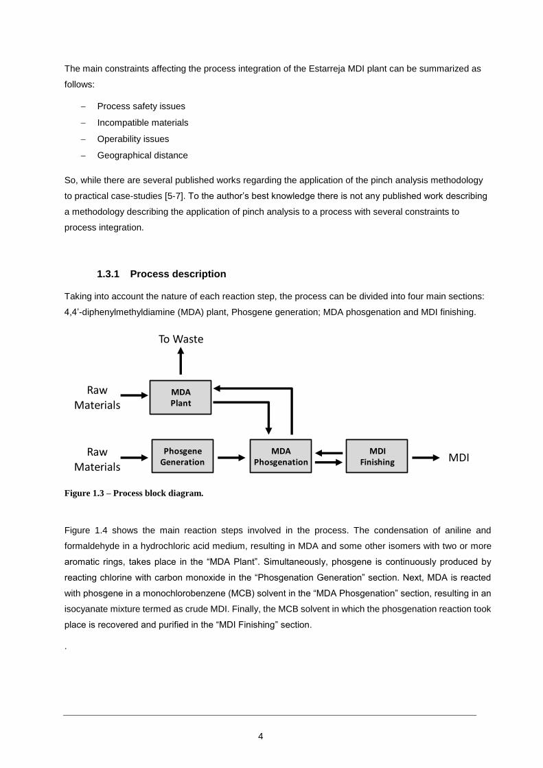
1.3.1 Process description

Taking into account the nature of each reaction step, the process can be divided into four main sections:

4,4’-diphenylmethyldiamine (MDA) plant, Phosgene generation; MDA phosgenation and MDI finishing.

Figure 1.3 – Process block diagram.

Figure 1.4 shows the main reaction steps involved in the process. The condensation of aniline and

formaldehyde in a hydrochloric acid medium, resulting in MDA and some other isomers with two or more

aromatic rings, takes place in the “MDA Plant”. Simultaneously, phosgene is continuously produced by

reacting chlorine with carbon monoxide in the “Phosgenation Generation” section. Next, MDA is reacted

with phosgene in a monochlorobenzene (MCB) solvent in the “MDA Phosgenation” section, resulting in an

isocyanate mixture termed as crude MDI. Finally, the MCB solvent in which the phosgenation reaction took

place is recovered and purified in the “MDI Finishing” section.

.

MDAPhosgenation

PhosgeneGeneration

MDIFinishing

MDAPlant

Raw Materials

Raw Materials

To Waste

MDI

5

Figure 1.4 – Main products and reaction steps involved in the MDI manufacturing process.

1.4 Thesis outline

This document is organized in 6 chapters and 3 appendixes. Apart from the thesis outline, Chapter 1

presents the motivation, scope and context for this study. In Chapter 2, an overview of the state of the art

methodologies used to evaluate and optimize the process energy efficiency is presented. An analysis of

the utility system, namely steam and cooling water systems, is performed in Chapter 3. Energy targets for

the hot and cold utilities are then presented in Chapter 4, where solutions to minimize energy consumption

are also shown. Finally, the main conclusions taken from this study and recommendations for future work

are given in Chapter 5. In Chapter 6 the references cited in this work are listed.

Appendix A1 has the equations and algorithms used for determining the psychometric data of air necessary

for the cooling tower simulations. Appendix A2 shows the equations used in the stream matching

methodology. In Appendix A3, the stream matching tools developed during this work are detailed.

In Figure 1.5, a word cloud with the terms used in this document is shown. The words that are most

frequently used are within the “thermal energy” context, which is in fact the main subject addressed in this

work.

Figure 1.5 – Word cloud with the terms using in this thesis.

Aniline MDA

NH2

2

H2C

H2N NH2

- H2O

+ CH2O

MDIH2C

OCN OCN

- 4 HCl

+ 2 COCl2

6

Figure 1.6 is a schematic representation of the thesis structure with a summary of the subjects addressed

in each chapter.

Figure 1.6 – Thesis structure and summary of each chapter.

Chapter 1 - Introduction

Summary Motivation, scope and industrial context behind this work are defined. The thesis structure is presented

Chapter 2 - Energy optimization overview

Summary An overview of the heat integration methodology for existent plants and a background review of each step of the methodology are detailed in this chapter.

Chapter 3 – Utility system analysis

Summary In this chapter the modeling, evaluation and optimization of the cooling water and steam system are explored.

Chapter 4 – Stream match methodology

Summary Using a new methodology, the industrial case-study energy targets are determined and alternative network configurations are detailed.

Chapter 5 - Conclusions and recommendations

Summary Main conclusions taken from this thesis as well as recommendation for future work are summarized in this chapter.

7

2 Energy efficiency optimization overview

This chapter details the energy efficiency optimization methodology and techniques. It starts by introducing

the energy optimization methodology for existent plants, listing the various steps. This is followed by the

presentation of key concepts related to each step of the methodology.

Nowadays, practically all manufacturing industries are challenged with increasingly high energy prices and

environmental regulations. An example of such regulations is the Kyoto Protocol, limiting the discharge of

greenhouse gases. The fact that carbon dioxide is considered one of the main greenhouse gases and the

energy sector is the primary source of carbon dioxide discharge implies that energy use is restricted as well

[6]. The petrochemical industry is especially sensitive to this issue as it is a very energy intensive sector.

Therefore, efforts to reduce energy consumption are being carried out not only in new plants but also in

existent ones.

Retrofitting/revamping a plant consists on analyzing an existing plant and evaluating whether it can be

improved, reducing energy consumption and emissions while increasing profitability. This process allows

the existent plants to remain competitive within the industry despite being originally designed with outdated

assumptions.

The purpose of this study is to present a methodology that can be used to evaluate and optimize the energy

performance of existent chemical manufacturing plants. The Estarreja PMDI plant is used as a case study

where the proposed methodologies are applied. Despite being a somewhat humorous image, Figure 2.1

represents the purpose of this work, i.e., an effort is taken to minimize the quality and quantity of the

resources that are used in the process, and therefore decreases waste as well, so that the operating costs

are reduced.

Figure 2.1 – An effort to reduce external utilities’ quality and quantity is constantly pursued.

Qu

alit

y (€

)

Quantity (€)

Waste

High quality resources

Process

8

Although the main aim of this work is the energy optimization of an existent plant using Heat Integration

techniques, a general note on Process Integration as boarder field study is recommended.

Process integration is a broad and active field that essentially aims for efficient use of raw materials and

energy, therefore reducing the environmental footprint.

The definition of Process integration, as stated by the International Energy Agency (IEA) [8] is as follows:

“Systematic and general methods for designing integrated production systems, ranging from individual

processes to total sites, with special emphasis on the efficient use of energy and reducing environmental

effects.”

The term Process Integration was widely diffused in the 1980’s mainly due to the introduction of the Pinch

concept by Linnhoff and his co-workers [9-11]. After the major advancements in Heat Integration that led

to significant improvements in the oil, chemical and power industries, further developments into other fields

followed. Due to the fact that the Pinch concept was initially applied to Heat Integration, the terms are

sometimes taken as identical. However, although Heat Integration is still today a major subject of the

Process Integration field (as shown in Figure 2.2), it is not exclusive. Nowadays, Process integration

methodologies also cover areas such as Mass Integration and Water Integration [12].

Figure 2.2 – Word cloud showing the prominence of the Keywords that appear more frequently in the works

returned by www.ScienceDirect.com with the search words “Process Integration” (August 2014).

9

The methodology followed in this work is presented in Figure 2.3 and is based on four main steps:

1. Data extraction – During this step, data was gathered either by direct measurements, design data

or simulation models. The ideal source of information is a process model properly validated with

plant data. Besides providing several operational parameters that in some cases are difficult to

obtain directly, it allows the evaluation of the impacts that the implementation of projects have on

the process. The outcome of this stage is therefore a set of process simulation models, validated

with plant data;

2. Utility system analysis – Models of the steam and cooling water network systems were developed.

The systems models allow the evaluation of the impacts that any process modification has on the

utility system. Additionally, they allow the identification of possible improvements on the utility

system itself.

3. Retrofit heat exchanger network – Based on stream material and energy balances, a retrofit

study was performed. The outcome of this stage is the cold and hot utility targets, current network

performance in relation to the targets and cross exchange possibilities;

4. Site improvements – Some of the alternatives generated during steps 2 and 3 are independent

from each other and some are not. Taking into account the various alternatives, several

combinations can be generated. The outcome of this stage is then a set of proposals with the

respective costs and savings estimates.

Project ideas generated by this methodology are then evaluated and, if implemented, will contribute to a

better energy efficiency of the site.

Figure 2.3 – Methodology for the overall process energy evaluation and optimization.

Retrofit Heat Exchanger Network

Site Improvements

Data Extraction

Utility System Analysis

10

2.1 Data extraction

Data extraction is the key link between the process and the evaluation/optimization steps that lead to site

improvements, the quality of the data collected during this phase is crucial for the validity of the subsequent

steps of the methodology.

The simulation tool used in this work was ASPEN PLUS [13], which is a software extensively used in the

petrochemical industry for steady state simulation and has been applied in feasibility studies of new

designs, analysis of complex plants with recycles and optimization [13]. This process simulator delivers a

comprehensive library of models that are user-editable as well as models that are organized by function,

such as Mixers/Splitters, Separators, Heat Exchangers, Columns, or Reactors, etc. Additionally, ASPEN

PLUS has a vast database of component properties along with an array of thermodynamic models that can

also be edited according to the user needs.

In regard to the property methods used in the models it is fundamental to choose the appropriate package.

Without quality input data and a good overall understanding of the modeled system from a chemical

engineering perspective, the simulation results can easily be misinterpreted. Kinetic data and

thermodynamic property methods can be the most likely source of error [14].

Regarding the Estarreja PMDI manufacturing plant, and before this study took place, process flowsheets

diagrams (PFD’s) as well as some ASPEN PLUS simulations were already available. These simulations

are a fair representation of the process as they have been validated with plant data; therefore, they were

used to perform the energy evaluation and optimization study.

Although it is possible to use only direct measurements, the ideal case is when this information is used to

validate process models. Consolidated process models can then provide a reliable source of information

for several operational variables and be used to evaluate the impact of the projects recommended by the

application of this methodology.

For performing an evaluation and optimization study of a process unit, it is necessary to simulate and

validate plant data. Simulation should provide a mass and energy balance consistent with plant

measurements. Nowadays, most of the processes are already simulated and validated with plant data.

However, it is important to cross-check all the available data to identify any inconsistency and correct it.

The importance of the simulation is not only to provide analysis data to the following stages of the study but

also to foresee the impact that any suggested modifications can promote on the process.

Although direct measurements portrait the process currently in operation, they may be inconsistent or

simply unavailable. In such cases the best option is to use design data to populate the simulations.

In modern manufacturing industries, computer aided engineering is present in practically all activities

related to process engineering. Flowsheeting is a key activity in process engineering and can be described

as the calculation of all output information and some internal variables using all information from the inputs

11

[15]. The architecture of a flowsheeting software is determined by the strategy of computation. Three basic

approaches have been developed over the years [16]:

- Sequential-Modular.

- Equation-Oriented.

- Simultaneous-Modular

In Sequential-Modular (SM) approach, the flowsheet model problem is partitioned into smaller (simpler)

sub-problems (Figure 2.4) [17]. Problem decomposition is based on the structure (topology) of the

flowsheet and is ideal for acyclic flowsheets (Figure 2.5.a).

Figure 2.4 – Sequential-Modular architecture diagram (Adapted from [17]).

In acyclic systems, i.e., without recycle streams (Figure 2.5.a), when the process feed streams and all the

unit and operating parameters are known, the SM approach is relatively straightforward as the units are

computed in a sequence where the output from one unit are the inputs for the next. In the example shown

in Figure 2.5.a, given Stream 1, Unit A would be the first to be solved; Stream 2 would then be used to

solve Unit B, and so on.

However, most processes involve recycles. Taking Figure 2.5.b as an example: Unit A could be directly

solved with only the input information (Stream 1); Unit B cannot be solved unless both Streams 2 and 6

are known; conversely Unit C cannot be solved until Stream 3 is determined.

A possible approach to solve this problem is to apply a tearing algorithm: 1. Tear (guess) the stream in the

recycle (Stream 6); 2. Perform a calculation pass through the flowsheet; 3. Evaluate the results by

comparing the calculated with the estimated value; 4. If it did not converge, replace the tear value by the

calculated value or by the average; 4. Iterate until convergence criteria are met.

Process model

Sub-problem2

Sub-problem1

Sub-problemn

Unit 1Unit 2

Unit n

Inp

ut

Ou

tpu

t

12

Figure 2.5 – Sequential modular approach (a) without recycle stream and (b) with recycle stream.

In Equation-Oriented (EO) approach, instead of tearing recycle streams and solving unit models in a

modular fashion the simulator assembles all the equations describing a process model and attempts to

solve them simultaneously.

Table 2.1 – Summary of characteristics of sequential-modular and equation-oriented architectures [15].

Sequential-modular Equation-oriented

Each unit operation is simulated sequentially All unit operations are simulated at once

The flowsheet is decomposed The equations are sorted

Iterative procedures using tear-streams All variables are updated at once

Less flexible but more robust More flexible but less robust

Initialization is important Initialization is very important

Memory requirements are not very high Memory requirements may be very high

In Simultaneous-Modular (SiM) approach, the solution strategy is a combination of Sequential-Modular

and Equation-Oriented approaches. Rigorous models are used at units' level, which are solved sequentially,

while linear models are used at flowsheet level, solved globally. The linear models are updated based on

results obtained with rigorous models. This architecture has been experimented in some academic

products. It may be concluded that SE approach keeps a dominant position in steady state simulation. The

EO approach has proved its potential in dynamic simulation, and real time optimisation. The solution for the

future generations of flowsheeting software seems to be a fusion of these strategies [16].

A B C D2 3 4 51

A B C D2 3 4 51

6

(a)

(b)

13

2.2 Utility system analysis

Although sometimes regarded as a minor component of the manufacturing process, utilities are often as

important as any other part of the technology as the savings achieved by an adequate design and operation

of the utility system can frequently surpass the ones achieved when modifying the process.

In the petrochemical and refining industries, cooling water and steam are arguably the most used utilities

for thermal energy distribution in the manufacturing processes [18] [19]. Water is often the preferred

medium for energy transport not only due to its relatively low cost and abundance but also because it is a

non-flammable and non-toxic resource .

The connection between the source/sink and the equipments that consume steam and cooling water is

established by means of a more or less complex distribution network [20]. These systems are often not

monitored and/or controlled, resulting in great material and energy waste. Modeling these systems can be

achieved by using computer-based mathematical models, allowing engineers to monitor the performance

of existent systems and create alternative operation scenarios.

While it is relatively common for process streams in chemical plants to have sufficient instrumentation, the

utility systems that support production are often not well monitored. This can make it impossible to

determine where unnecessary consumption or leaks are occurring. This work will provide essential

information for identifying utility consumption and enable strategies to save energy and to improve

efficiency.

To overcome the current high energy costs, refiners and petrochemical producers are looking for ways to

improve their energy efficiency and reduce these unnecessary energy costs. Utility systems are

characterized by a branched piping network, sending steam, air, water, electricity, etc. to and from the

process units [21]. Often only the network’s main headers and branches are instrumented, which leaves

many areas unmonitored. This limited coverage may help calculate the overall consumption and identify

the main suppliers’ and consumers’ performance, but it does not help close the material balance or identify

possible leaks or wasted use. Engineers also do not have enough information to optimize the usage of

these utilities across the site.

In regard to the systems optimization, although several different methods for energy systems analysis are

available, often they can only be applied when designing a heat recovery network without any plant layout

considerations. It is, however, not very often that new plants are built; instead, retrofitting of existing

processes is carried out. The extreme case would be to remove all existing equipment and build a new

optimized process from scratch, but this would result into significant capital waste. When retrofitting a

system, already installed equipment must be taken into account as it represents sunken capital. On the

other hand, the thermal and hydraulic impact that any modification has on the rest of the network must be

carefully analyzed.

14

2.2.1 Cooling water system

The cooling water system in an industrial facility that usually comprises the cooling tower and the cooling

water network. The cooling tower is responsible for rejecting waste energy to the environment by means

of evaporative cooling. The cooling water network is essentially a heat exchanger network that is used for

removing waste heat from the process.

Cooling towers

Cooling towers are widely employed in many industrial applications for rejecting waste heat from the

process to the environment. The principle behind a cooling tower operation is evaporative cooling which, in

theory, would allow circulating water to equal ambient air wet-bulb temperature. Evaporative cooling is a

process with simultaneous mass and heat transfer between air and circulating water.

There are several methods and strategies related to the modeling of cooling towers with different levels

of complexity. According to Jin et al. [22], the first theoretical analysis of cooling towers was performed by

Dr. Fredrick Merkel in 1925. He proposed a theory relating evaporation and sensible heat transfer where

there is counter flow contact of water and air. As described by Benton et al. [23], Merkel expressed the

number of transfer units (NTU) as a function of the integral of the water temperature difference divided by

the enthalpy gradient where, to reduce the governing relationships to a single separable ordinary differential

equation, several simplifying assumptions were made: Merkel assumed that the Lewis factor, relating heat

and mass transfer was equal to 1; the air exiting the tower was saturated with water vapor; and the reduction

of water flow rate by evaporation was neglected in the energy balance.

Kloppers and Kröger [24] evaluated three methods used in cooling tower design, namely, Merkel, Poppe

and effectiveness-NTU and gave a detailed derivation of the heat and mass-transfer equations of

evaporative cooling in cooling towers. Based on Merkel equation, Picardo and Variyar [25] presented a

power law that related packed height with excess air and determined equation parameters for air wet-bulb

temperature between 10–34 ºC and cooling range between 40–20 ºC. They also showed that beyond a

certain air flow the reduction in packed height does not justify the increase in energy utilization for air

compression.

Castro et al. [26] developed an optimization model for a cooling water system composed of a counter flow

tower and five heat exchangers where the thermal and hydraulic interactions in the overall process were

considered. They observed that forced withdrawal of water upstream of the tower is an important resource

for fulfilling cooling duty requirements. Khan et al. [27] presented a fouling growth model where it was

demonstrated that the effectiveness of a cooling tower degrades significantly with time, indicating that for

a low fouling risk level (p = 0.01), which is the probability of fill surface being fouled up to a critical level

after which a cleaning is needed, there is about 6.0% decrease in effectiveness. Al-Waked and Behnia [28]

applied computational fluid dynamics (CFD) for natural draft wet cooling tower. The difference between

outlet air temperature predicted by the CFD model and design results was less than 3%. Jin et al. [22]

proposed a model based on heat resistance and energy balance principles where empirical parameters

were introduced, avoiding the need to specify geometrical parameters. Rubio-Castro et al. [29] determined

15

optimal cooling tower design parameters and temperature profiles across a counter flow cooling tower by

applying a rigorous heat and mass transfer model. Nonlinear algebraic equations were solved using a

discretization approach with a fourth-order Runge-Kutta algorithm. Given a set of experimental data to train

the model, Hosoz et al. [30] suggested that applying artificial neural networks (ANN) for modeling the

cooling tower performance avoided the solution of complex differential equations. Predicted and

experimental values had correlation coefficients in the range of 0.975–0.994 and mean relative errors in

the range of 0.89–4.64%. Pan et al [31] presented a data-driven model-based assessment strategy to

investigate the performance of an industrial cooling tower. Considering one month test interval and based

on water mass flow rate, water inlet temperature, air dry-bulb temperature, relative humidity and fan motor

power consumption the predicted water outlet temperature was within a ±5% error band and presented a

mean square error of 0.29 ºC. Serna-González et al. [32] used mixed-integer nonlinear programming

(MINLP) techniques to evaluate the optimal conditions of a mechanical draft cooling tower that minimize

the total annual cost for a given heat load, dry- and wet-bulb inlet air temperatures and temperature

constraints on the cooling water network. Rao and Patel [33] compared the results obtained by Serna-

González et al. [32] with the ones achieved when applying an artificial bee colony algorithm. Using the

artificial bee colony algorithm resulted in an objective function value lower than the one achieved by Serna-

González et al. [32] for all six case studies (improvement between 1.27% and 11.17%).

Xiaoni et al. [34] studied and developed a mathematical model of a seawater shower cooling tower and

although the cooling performance decreases with increased salinity and is not as high as when compared

to “freshwater” cooling towers, seawater is more readily available than freshwater in important chemical

clusters around the world. On another study that uses seawater as a cooling medium, Sadafi et al. [35]

investigated the spray nozzle configuration and established a dimensionless correlation to predict the

distance from the nozzle after which the dry stream starts (wet length) and cooling efficiency.

As an alternative to the abovementioned methodologies, a different approach that does not involve the

solution of differential equations can be used to model a cooling tower operation by applying an equilibrium

stage. While the equilibrium stage method can hardly be used for design purposes without proper

correlations that allow the determination of the height equivalent to a theoretical plate (HETP), it is

demonstrated in this work that both the outlet water and air temperature predicted by the model are quite

accurate when compared to the experimental values.

Cooling Water networks

Cooling water networks have been studied in the past due to their importance in most industrial processes.

The structure of a cooling water network influences the operation of the cooling tower as cooling water flow

and cooling tower inlet temperature are variables that directly impact on the cooling tower performance.

Thus, optimizing the cooling water network allows designing a cooling water network that eventually leads

to requiring a lower capacity cooling tower, involving a lower capital investment. This can be of paramount

importance in grassroot design or when retrofitting an existent plant with limited cooling tower capacity.

16

Kim and Smith [19] developed a methodology based on pinch technology that provided design guidelines

for cooling water system design. In retrofitting situations, they concluded that better design of the cooling

network, increasing cooling tower blowdown, taking hot blowdown and strategic use of air coolers, could

be used to avoid investment in new cooling tower capacity.

Ponce-Ortega et al. [36] presented a mixed-integer nonlinear programming (MINLP) algorithm for the

synthesis of cooling networks. The strategy was based on a superstructure that allowed a combination of

arrangements in series and in parallel, considering simultaneously the capital cost for the coolers and the

utility costs.

Gololo and Majozi [37] study focused mainly on cooling systems consisting of multiple cooling towers that

supplied a common set of heat exchangers. The heat exchanger network was synthesized based on a

mathematical optimization technique that defined a superstructure in which all opportunities for cooling

water reuse were explored. They applied the proposed methodology to two case studies, rendering MINLP

and NLP problems, depending on whether a cooling tower could supply only a dedicated set of coolers,

MILNP problem, or could supply any coolers of the network, NLP problem.

A two-step methodology for the optimization of a cooling water network was developed by Sun et al. [38].

The first step of the methodology was to use a thermodynamic model to obtain an optimal cooler network

and a second step, where the hydraulic model was established to obtain the optimal pump network with

auxiliary pumps installed in parallel branch pipes. The authors identified savings of up to 23.3% of the cooler

network cost and 11% of the pump network cost.

A numerical hydraulic model of a cooling water system in EPANET was built by Georgescu et al. [39]. Since

EPANET does not have the possibility to insert some equipment into the network such as heat exchangers

they used throttle valves with adjusted loss coefficients to simulate these equipments and account for their

pressure drop. They adjusted the model with pressure loss measurements and concluded that the resulting

model fitted field data.

The approach suggested in this work resulted from a combination of the cooling water hydraulic model, to

determine the cooling water flow on each point of the network, and the thermodynamic model, to calculate

the cooling water temperature on each point. The models allow a precise simulation of the cooling water

network and serve as a basis for performing modification studies on the cooling water heat exchanger

network.

2.2.2 Steam system

Steam is widely used within the chemical industry as medium to distribute thermal energy across the various

process units. A steam system comprises steam generators where energy from any given source is

transferred to water and steam is generated. Although the energy required to generate steam can be

supplied by a variety of sources, such as an electric current passing through a resistance, solar and

17

geothermic energy, etc., within the chemical industry the energy is commonly provided either by burning

fuel or cooling down a process stream.

The steam generated in the steam generator is then fed to a network where it is distributed to the various

consumers. It is not uncommon to have a network where steam is distributed at different pressure and

temperature levels. Steam is then either injected directly into the process or condensed in heat

exchangers. Condensates can then be flashed to generate steam at a lower pressure or return to the

steam generator.

Steam generator

As mentioned above, steam can be generated from various sources, being that the most common in

process industries is that the energy is provided by either burning fuel or cooling down a process stream.

Fired steam boilers are used to produce steam by using the energy released by fuel combustion. Several

parameters influence boiler efficiency and can therefore be optimized. These parameters are discussed

elsewhere in Section 3.2, where a detailed analysis of boilers performance is presented.

Artificial neural networks (ANN) were applied by Kljajic et al. [40] to forecast the performance of fired boilers.

They stated that the most influential parameters on boiler efficiency were oxygen content in flue gas, boiler

maximum capacity and boiler load. Behera et al. [41] also used ANN to predict the performance of a refuse

plastic fuel (RPF) boiler. Based on feed water pressure, feed water temperature, fuel conveyor speed, and

incinerator exit temperature they were able to estimate the steam temperature, pressure, and mass flow

rate. A different work developed by Strušnik et al. [42] where ANN were applied to develop a model that

predicts the power production of a power plant and distributes the production between the boilers so that

the latter operate at their highest efficiency.

Andreassen and Olsen [43] used mathematical optimization tools to solve a load allocation problem with

minimum cost as the objective function. Given a certain steam demand in a plant with more than one boiler

supplying the steam network, the method allowed the optimum load allocation to each boiler so that the

operating cost was minimal. They applied the methodology to a paper mill case study where it was

demonstrated that the optimum load optimization strategy gave tangible savings when compared to the

equal load distribution strategy.

A study where an algorithm based on a second-order gradient search method that optimize the allocation

of multiple industrial boilers consuming single or multiple fuel types was presented by Dunn and Du [44].

They showed through a variety of practical examples that the proposed methodology was capable of

producing more favorable results in terms of operating costs than the base case scenario.

To support fuel management decisions in the steam production system of industrial boilers Rocco and

Morabito [45] proposed a MILP model. The model covers variables such as fuel replenishment and its

inventory control), boiler operational decisions (start-up, warm-up, and shutdown operations) and which

boiler should produce steam.

18

Differently from the abovementioned approaches this work describes a methodology for optimizing the

boiler load in a multi-boiler steam system. The load allocation of each boiler depends on the thermal

efficiency of the boiler and plant demand.

Steam network

The steam network consists on the distribution network of steam supply to the various users and the

subsequent return of condensates to the steam generator. In large industrial plants steam is usually

distributed at different pressure and temperature levels.

A mathematical approach for retrofit and optimization of total site steam distribution networks was

developed by Chen et al. [46]. The MILNP formulation rendered a model where retrofit solutions of an inter-

plant steam network were effectively achieved. They investigated the operational optimization of existing

units, installation of new turbines, replacement of low-efficiency boilers and turbines and use of steam

ejectors to upgrade a low pressure steam current to a level where it could be used in the plant.

Majane [47] presented a Model Predictive Control method (MPC) for pressure control of steam systems. A

power plant simulator controlled by MPC helps to decide the location and the capacity of steam levelling

components needed to stabilize the operation of the process.

Process integration techniques were used by Coetzee and Majozi [48] to study the steam system network

synthesis. Their approach consisted on a hybrid method that combined pinch technology and mathematical

optimization that minimized the steam flow. This was achieved by placing heat exchangers in series instead

of the typical parallel configuration. By placing the heat exchangers in series it allows hot condensates to

heat cold streams instead of using always steam.

Zhong et al. [49] proposed a hydraulic model of a steam network that took into consideration heat

dissipation in pipes. The authors used the software HEATNET to build the simulation and introduced a

control strategy to avoid steam stagnation by optimizing the heat load distribution.

In this work, a methodology for building a thermodynamic model of the steam network in ASPEN PLUS is

described. This methodology describes the implementation of a model of the steam network that can then

be used as a basis for optimization studies and for the evaluation of the impacts that any modification has

on the overall balance of the steam network.

2.3 Retrofit heat exchanger networks

With the formalization of the pinch point concept by Umeda et al. [50] and Linnhoff and Flower [10, 11] in

the late 1970’s, it was possible to quantify the maximum recoverable heat and the minimum utilities

requirement. The “best” heat exchanger network design that allows these targets to be met is yet another

19

problematic point as there is a trade-off between energy, heat transfer area and number of heat transfer

units, as pictorially shown in Figure 2.1.

Figure 2.6 – Trade-offs in heat exchanger network design (Adapted from Yee and Grossman [51]).

Ever since the first developments in the heat exchanger network synthesis introduced by Linnhoff et al. in

1978 [9-11], several new extensions were introduced, incorporating existent and new methodologies into

other process synthesis problems such as heat exchanger network retrofit.

According to Nordman [52], early approaches were mainly based on synthesis methods that were originally

aimed for grass-root design. The retrofit methodologies usually consisted on generating grass-root designs

and then selecting the design closest to the existing one for further development.

Retrofit methodologies can be clustered into pinch analysis methods, mathematical programming or a

combination of both:

Pinch analysis methods use pinch analysis to solve retrofit problems. They employ the typical pinch tools

such as composite curves, grand composite curves, etc., to retrofit heat exchanger networks. The retrofit

process based on pinch methodologies rely on a strong user interaction. Although this can be an advantage

in some cases, it can be very time consuming. Additionally, because heuristics play a major role during the

process, the end result is strongly dependent on the user’s experience and good judgment.

Mathematical programming methods comprise the solution of a mathematical model formulation using

optimization methods. Considering network topology modifications such as stream splits, heat exchanger

relocation or new exchanger as being subject to optimization renders a Mixed Integer problem. Moreover,

the area equations that use the Log Mean Temperature difference (LMTD) are intrinsically non-linear. Thus,

due to the aforementioned reasons, HEN retrofit is by nature formulated as Mixed Integer Non-Linear

Programming (MINLP) problem. To overcome the inherent complexity of the MINLP problem, the

formulation is usually simplified as Mixed Integer Linear Programming (MILP), Non-Linear Programming

(NLP) or Linear Programming (LP) by making some assumptions and step-wise manipulation. As an

alternative to deterministic methods that are often trapped at a local optimum, stochastic methods such as

simulated annealing algorithms and genetic algorithms, are also employed [53]. As stated on the review of

heat exchanger retrofit methodologies presented by Sreepathi and Rangaiah [54], mathematical

UtilityConsumption

Number of Units

Area

20

programming based methods are popular in academia but much less so in industrial practice due to the

difficulty of setting up the problem models, particularly for practitioners.

Hybrid methods are the methods that make use of both pinch analysis and mathematical programming in

an effort to combine the strengths of both. They allow user interaction and can also be applied to large

problems.

2.3.1 Pinch analysis

As previously mentioned, pinch analysis was conceived greatly due to the contributions of Linnhoff and his

co-workers at the Leeds University [9-11] in the late 1970’s, with Imperial Chemical

Industries (ICI) pioneering in the use of this technology [55]. Although pinch analysis was initially targeted

for energy optimization applications, the concept was successfully translated to other fields such as

wastewater minimization and other mass exchange networks and hydrogen pinch [56-58].

The objective of applying pinch analysis is to reduce the consumption of a given resource through process

integration, usually thermal energy. It can be used during the design phase, where the heat exchanger

network is configured so that the hot and cold utility consumption is minimized, or to retrofit existent units,

which is achieved by evaluating how efficiently a resource is being used and what actions should be taken

to close the gap between current consumption and the minimum consumption targets. The targets given

by pinch analysis are conceptual and can hardly be achieved in a complex industrial process. Nonetheless,

they set the goal for external resource consumption, giving an important incentive to find a network that is

as close to this values as possible.

Kemp [55] summarized three different approaches for heat exchanger network retrofit using pinch analysis:

1. Develop a Minimum Energy Requirement (MER) heat exchanger network design as for a new plant but,

where an option exists, select matches which already exist in the current network. This was the approach

used in the earliest pinch studies;

2. Start with the existing network and work towards a MER design. Take the current ΔTmin and calculate

the targets and the pinch temperature. The existing exchangers, heaters and coolers are plotted on the

grid diagram and the pinch violators are identified. Finally, alternative configurations that add new matches

which correct these problems are identified. This approach was described by Tjoe and Linnhoff [59];

3. Start with the existing network and identify the most critical changes required in the network structure

to give a substantial energy reduction. This method will be appropriate if the MER design is so different in

configuration from the existing layout that they are virtually incompatible.

Tjoe and Linnhoff [59] presented the first application of pinch tools to heat exchanger network retrofit,

developing the concept of area efficiency in heat exchanger networks, α. Area efficiency is the ratio between

the area of an existent network and, assuming the same energy consumption as the existing network, the

area that would be required if the network was designed so that there was no crisscross heat transfer, i.e.,

only vertical heat transfer was allowed . The method assumes that the area efficiency of the retrofit HEN is

equal to that of the existing network, and this assumption is used to set targets for design [60].

21

The Cost Matrix approach presented by Carlsson et al. [61] takes into account the cost of structural changes

implemented in the retrofit design, but it depends on accurate piping and other cost data for each potential

match. According to Asante et al. [62], this methodology can be impractical in some cases, stating that

considerable effort would is required to generate the necessary data for a moderately sized industrial

process.

Pinch concepts

Within a process, there are some streams that need to be cooled down and others heated up. A stream

that is at a given temperature and is heated up is defined as being a cold stream, whereas a stream that

is cooled down is defined as a hot stream.

Heat can be supplied or removed from the process through the use of external utilities. They can be hot

utilities (e.g. steam, hot oil, combustion gases) or cold utilities (e.g. cooling water, air, refrigeration fluid).

It was previously mentioned that pinch analysis produced a set of energy targets. This is in fact an

important concept in pinch analysis. These targets refer to the thermodynamic targets that the process

would meet if it was perfectly integrated. There are three important targets given by the heat pinch analysis:

cold utility; hot utility and cross-exchange targets. The aim of the pinch engineer is then to identify the best

network configuration that enables the process to move closer to these targets.

Another key concept of pinch analysis is the one of pinch point, often referred simply as “pinch”. This

concept relates to the most constrained region of a heat exchanging network, i.e., nowhere else than at this

point does the minimum approach, ΔTmin, occurs [9]. Once the pinch point has been identified, it is possible

to consider the process as two separate systems: one above and one below the pinch.

Based on the concepts described above, for a process to achieve minimum energy targets, pinch

methodology states that three fundamental rules must be obeyed:

1. Heat must not be transferred across the pinch;

2. There must be no external cooling above the pinch;

3. There must be no external heating below the pinch.

22

Temperature – Enthalpy representation

The T-Q diagram is very useful in the pinch analysis methodology as it provides a visual representation of

the streams’ energy and temperature variation.

A variable described as the heat capacity flow rate, CP (kW.ºC-1), is introduced. This variable is considered

as constant for each stream and is given by Equation (2.1), which is the product between the mass flow

rate, M (kg.s-1), and the specific heat capacity at constant pressure Cp (kJ.kg-1.ºC -1).

𝐶𝑃 = 𝑀 × 𝐶𝑝

(2.1)

The term “enthalpy”, Q (kW), refers to the differential heat flow between the stream inlet and outlet stream

conditions. It is given by Equation (2.2), which is the product between MCp and the difference between the

inlet, Tin (ºC), and outlet, Tout (ºC), temperatures.

𝑄 = 𝐶𝑃(𝑇𝑜𝑢𝑡 − 𝑇𝑖𝑛)

(2.2)

In a T-Q plot where temperature, T, is in the vertical axis and enthalpy, Q, the horizontal axis. Since enthalpy

is a property that results from the difference between two thermodynamic states, the line segment can be

drawn anywhere in the enthalpy axis as long as each stream is represented by a line segment with slope

MCp, that starts on Tin and finishes on Tout.

For two streams to cross-exchange there must be a temperature drive between the two and the hot stream

must be hotter than the cold stream. So, in the T-Q plot, the hot stream must at all times be above the cold

stream at a distance of at least ΔTmin.

In Figure 2.7, an example of a countercurrent heat exchanger is shown. A hot stream enters the heat

exchanger at THin with a target temperature of THout and the cold stream enters the heat exchanger at TCin

with a target temperature of TCout. Heat recovery reaches its maximum when the approach between the hot

outlet and the cold inlet temperature is equal to ΔTmin. If this temperature approach was to be increased to

ΔT> ΔTmin, the curves would be shifted (dashed line in Figure 2.7) and external utilities would be required.

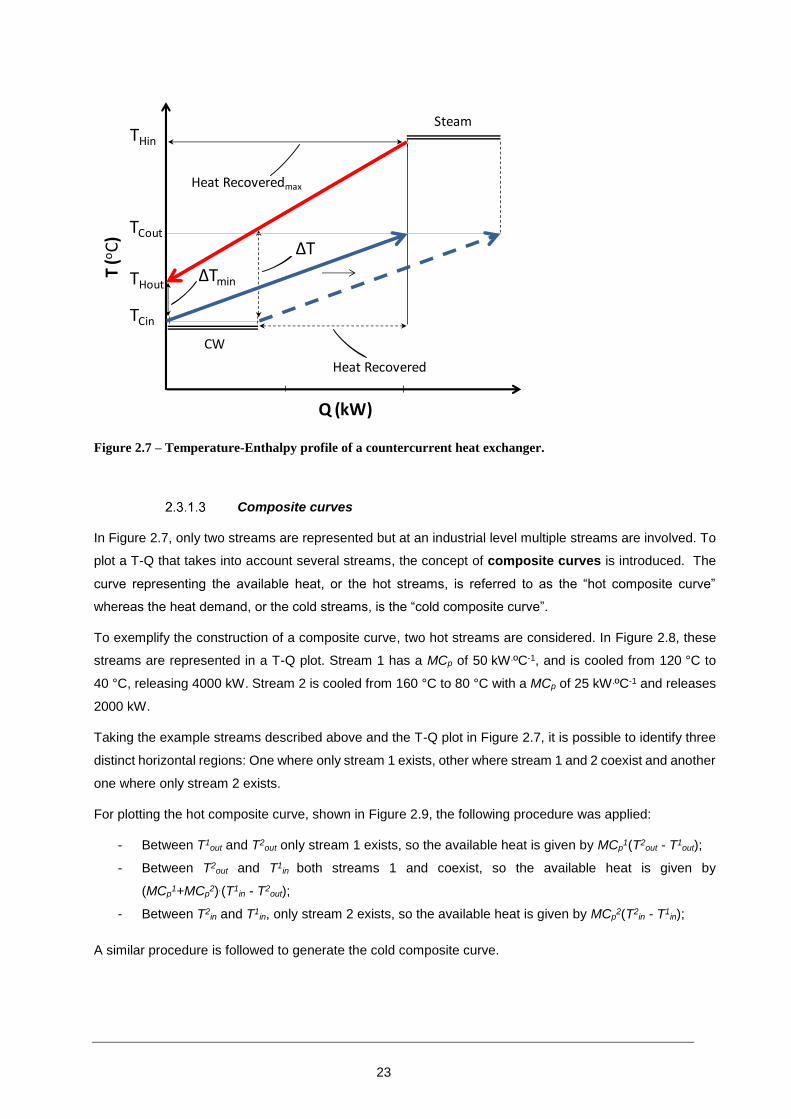
23

Figure 2.7 – Temperature-Enthalpy profile of a countercurrent heat exchanger.

Composite curves

In Figure 2.7, only two streams are represented but at an industrial level multiple streams are involved. To

plot a T-Q that takes into account several streams, the concept of composite curves is introduced. The

curve representing the available heat, or the hot streams, is referred to as the “hot composite curve”

whereas the heat demand, or the cold streams, is the “cold composite curve”.

To exemplify the construction of a composite curve, two hot streams are considered. In Figure 2.8, these

streams are represented in a T-Q plot. Stream 1 has a MCp of 50 kW.ºC-1, and is cooled from 120 °C to

40 °C, releasing 4000 kW. Stream 2 is cooled from 160 °C to 80 °C with a MCp of 25 kW.ºC-1 and releases

2000 kW.

Taking the example streams described above and the T-Q plot in Figure 2.7, it is possible to identify three

distinct horizontal regions: One where only stream 1 exists, other where stream 1 and 2 coexist and another

one where only stream 2 exists.

For plotting the hot composite curve, shown in Figure 2.9, the following procedure was applied:

- Between T1out and T2

out only stream 1 exists, so the available heat is given by MCp1(T2

out - T1out);

- Between T2out and T1

in both streams 1 and coexist, so the available heat is given by

(MCp1+MCp

2).(T1in - T2

out);

- Between T2in and T1

in, only stream 2 exists, so the available heat is given by MCp2(T2

in - T1in);

A similar procedure is followed to generate the cold composite curve.

Q (kW)

THin

THout

TCout

TCin

T (o

C)

CW

Steam

Heat Recovered

Heat Recoveredmax

ΔTmin

ΔT

24

Figure 2.8 – Two hot streams represented in the T-Q plot.

Figure 2.9 – Stream 1 and 2 combined in one single composite curve.

In Figure 2.10, hot and cold composite curves are combined in the same T-Q plot. This is achieved by

positioning the left edge of the hot composite curve at Q = 0 and shifting the cold composite curve until the

gap between the two curves equals ΔTmin.

Q (kW)

40

80

T (o

C)

120

160

02000 4000 6000

Stream 1MCp = 50 kW/oCΔQ = 4000 kW




Q (kW)

40

80

T (o

C)

120

160

02000 4000 6000

25

Figure 2.10 – Hot and cold composite curves in the same T-Q plot.

By combining the hot and cold composite curves in a single T-Q plot it is possible to determine the amount

of heat recovered as well as the external utilities requirements. In Figure 2.11, the shaded area where the

hot and cold composite curves coexist correspond to the total recoverable heat whereas the region where

only the hot and cold curves exist correspond to the external cold and hot utility requirements, respectively.

Figure 2.11 – Energy targets given by the combined composite curves.

ΔTmin

PINCH

Hot Composite Curve

Cold Composite Curve

Q (kW)

40

80

T (o

C)

120

160

02000 4000 6000

QCmin

QHminHeat Recovered

40

80

T (o

C)

120

160

02000 4000 6000

26

Grand Composite Curve (GCC)

In most processes, heating and cooling are performed by using different utility levels (e.g. different steam

levels, hot oil, cooling water, air, refrigeration). Since lower level utilities (closer to ambient conditions) are

cheaper than higher level utilities (e.g. cooling water is cheaper than refrigeration), consumption of higher

level utilities should be minimized by using lower level utilities, wherever it is viable.

Although composite curves are useful to determine the overall energy targets, they are hardly the best tool

for identifying multiple utility targets. Conversely, The Grand Composite Curve (GCC) is a very convenient

tool for setting the targets for the multiple utility levels.

(a) (b)

Figure 2.12 – Composite curve shifting.

(a) (b)

Figure 2.13 – Construction of the grand composite curve.

T (o

C)

Q (kW)

QCmin

Qhmin

PINCHT s

hif

ted(o

C)

Q (kW)

QCmin

Qhmin

PINCH

α

Shifted down by ½ ΔTmin

Shifted up by ½ ΔTmin

T sh

ifte

d(o

C)

Q (kW)

QCmin

Qhmin

PINCH

T sh

ifte

d(o

C)

Q (kW)

QCmin

Qhmin

α α

27

(a) (b)

Figure 2.14 – Grand Composite Curve used to determine utility targets in (a) a process with only two utility

levels and (b) a process with multiple utilities levels.

Figure 2.15.a shows an example of perfectly integrated process i.e., no heat transferred across the pinch

and no cooling or heating above and below the pinch, respectively, as stated by the pinch rules.

In Figure 2.15.b, α amount of heat is transferred from above the pinch to below the pinch. The system

above the pinch, which was before in heat balance with QHmin, now loses α units of heat to the system below

the pinch. To restore the heat balance, the hot utility must be increased by the same amount, that is, α

units. Below the pinch, α units of heat are added to the system that had an excess of heat, therefore the

cold utility requirement also increases by α units. In conclusion, the consequence of a cross-pinch heat

transfer (α) is that both the hot and cold utility will increase by the cross-pinch duty (α).

Figure 2.15.c also shows γ amount of external cooling above the pinch and β amount of external heating

below the pinch. The external cooling above the pinch of γ amount increases the hot utility demand by the

same amount. Therefore, on an overall basis both the hot and cold utilities are increased by γ amount.

Similarly, external heating below the pinch of β amount increases the overall hot and cold utility requirement

by the same amount (i.e. β).

T shif

ted(o

C)

Q (kW)

Refrig.

HP

T shif

ted(o

C)

Q (kW)

Refrig.

HP

MP

CW

28

(a)

(b) (c)

Figure 2.15 – Hot and cold composite curves for: (a) a process with minimum energy requirements, (b) a

process where α amount of heat is transferred across the pinch and (c) a process with γ amount of external

cooling and β amount of external heating above and below the pinch, respectively.

2.3.2 Mathematical programming

Cerda et al. [63] formulated an algorithm as a “transportation” problem, a well-known problem for which

efficient algorithms exist, that allowed the minimum utility calculation for a heat exchanger network

synthesis. In order to find the smallest number of matches in the process, a MILP model was relaxed into

a linear programming “transportation” problem and solved. Later, Cerda and Westerberg [64] extended

their work by formulating an algorithm that allowed the user to impose constraints disallowing the matching

of stream pairs.

Papoulias and Grossman [65] proposed a similar approach by formulating a MILP problem based on

“transshipment” models, being a considerably smaller variation of the “transportation” model, which was

used for deriving network configurations. The minimum number of matches that should take place in the

network is determined by means of the “transshipment” model involving the solution of a MILP, by means

of a branch-and-bound method. The heat exchanger network configuration is not obtained directly from the

QCmin

Qhmin

PINCH

Zero

T (o

C)

Q (kW)

QCmin + α

QHmin + α

Infeasible

T (o

C)

Q (kW)

PINCH

Zero

QCmin + β

QHmin + γ

γ

β

T (o

C)

Q (kW)

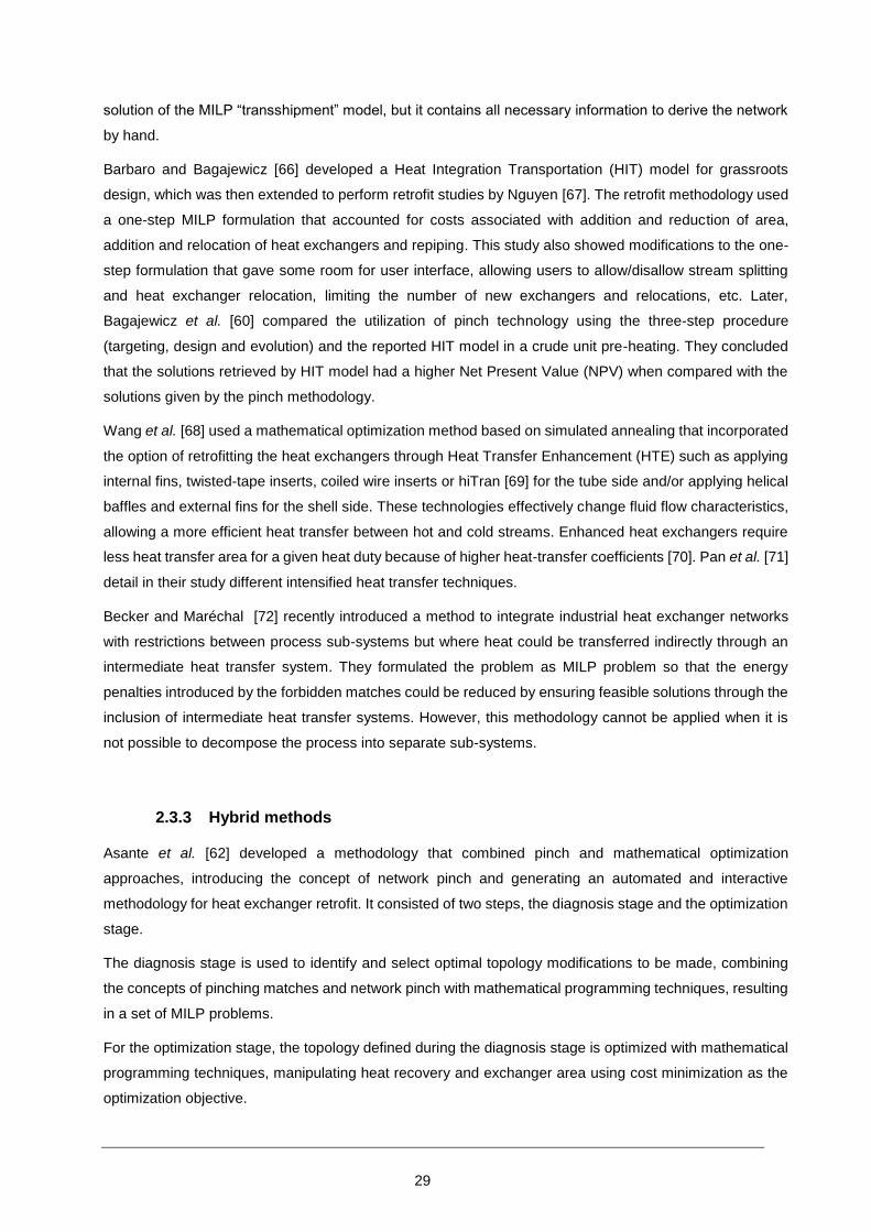
29

solution of the MILP “transshipment” model, but it contains all necessary information to derive the network

by hand.

Barbaro and Bagajewicz [66] developed a Heat Integration Transportation (HIT) model for grassroots

design, which was then extended to perform retrofit studies by Nguyen [67]. The retrofit methodology used

a one-step MILP formulation that accounted for costs associated with addition and reduction of area,

addition and relocation of heat exchangers and repiping. This study also showed modifications to the one-

step formulation that gave some room for user interface, allowing users to allow/disallow stream splitting

and heat exchanger relocation, limiting the number of new exchangers and relocations, etc. Later,

Bagajewicz et al. [60] compared the utilization of pinch technology using the three-step procedure

(targeting, design and evolution) and the reported HIT model in a crude unit pre-heating. They concluded

that the solutions retrieved by HIT model had a higher Net Present Value (NPV) when compared with the

solutions given by the pinch methodology.

Wang et al. [68] used a mathematical optimization method based on simulated annealing that incorporated

the option of retrofitting the heat exchangers through Heat Transfer Enhancement (HTE) such as applying

internal fins, twisted-tape inserts, coiled wire inserts or hiTran [69] for the tube side and/or applying helical

baffles and external fins for the shell side. These technologies effectively change fluid flow characteristics,

allowing a more efficient heat transfer between hot and cold streams. Enhanced heat exchangers require

less heat transfer area for a given heat duty because of higher heat-transfer coefficients [70]. Pan et al. [71]

detail in their study different intensified heat transfer techniques.

Becker and Maréchal [72] recently introduced a method to integrate industrial heat exchanger networks

with restrictions between process sub-systems but where heat could be transferred indirectly through an

intermediate heat transfer system. They formulated the problem as MILP problem so that the energy

penalties introduced by the forbidden matches could be reduced by ensuring feasible solutions through the

inclusion of intermediate heat transfer systems. However, this methodology cannot be applied when it is

not possible to decompose the process into separate sub-systems.

2.3.3 Hybrid methods

Asante et al. [62] developed a methodology that combined pinch and mathematical optimization

approaches, introducing the concept of network pinch and generating an automated and interactive

methodology for heat exchanger retrofit. It consisted of two steps, the diagnosis stage and the optimization

stage.

The diagnosis stage is used to identify and select optimal topology modifications to be made, combining

the concepts of pinching matches and network pinch with mathematical programming techniques, resulting

in a set of MILP problems.

For the optimization stage, the topology defined during the diagnosis stage is optimized with mathematical

programming techniques, manipulating heat recovery and exchanger area using cost minimization as the

optimization objective.

30

3 Utility system analysis

This chapter presents the modeling and evaluation of the cooling water and steam systems of the case

study plant. By using the methodology described in this chapter it is possible to evaluate the performance

of the current network as well as providing a tool for evaluating any plant modification that impacts on the

utility systems.

The cooling water system described in this chapter is composed by the cooling water network, where waste

heat of the process is throw out to the cooling water, and the cooling tower, where the heat is dissipated to

the environment. For determining the flow on each heat exchanger a hydraulic model was implemented

and for determining the temperatures on each point of the network as well as the behavior of the cooling

tower a thermodynamic model was implemented.

3.1 Cooling water system

To determine the flow on each point of the cooling water network a hydraulic model was implemented.

Then, to simulate the cooling water system thermodynamic behavior, a methodology for modeling with

ASPEN PLUS an existent cooling tower and the cooling water network is presented. Finally, the

performance of the cooling water system is evaluated.

3.1.1 Hydraulic model of cooling water network

The cooling water network consists on all the heat exchangers where cooling water is used to remove heat

from the process. Cooling water then goes through the cooling tower, where waste heat is rejected to the

environment.

Cooling tower performance depends on several parameters, where both inlet water temperature and flow

are two important variables. On the other hand, they depend on the cooling water network configuration

and duty. As a result, two approaches were considered for modeling the cooling water network and are

presented as follows: Hydraulic simulation and thermodynamic simulation.

While hydraulic simulation provided with an estimate for the flow of cooling water going through each heat

exchanger, thermodynamic simulation was used to determine the temperature on each point of the network.

The inputs for the models were the network configuration together with each heat exchanger heat duty and

cooling tower performance.

The Estarreja MDI plant cooling water network has a parallel arrangement, i.e., fresh cooling water passes

through each heat exchanger only once before returning to the cooling tower. After being cooled down in

31

the cooling tower, cooling water goes through three parallel pumps that feed a main supply duct. Heat

exchangers are located between the supply and return ducts so that cooling water flows between them.

For the hydraulic simulation of the Estarreja MDI plant the SiNET software [73] was used. SiNET is a

software tool developed by Epcon that allows the user to model complex liquid and gas networks in regard

to the fluid hydraulic behavior. It computes the head loss imposed by pipe friction and fittings as well as

pressure drop caused by pieces of equipment such as heat exchangers. For a given network configuration

and pump curves, SiNET computes pressure and flow at each node of the network for a stated set of

pressure and flow inputs.

A detailed survey of the cooling water network was carried out, resulting in the mapping of the network in

terms of pipe length, size, elevation and fittings. The information related with piping configuration was

retrieved from isometric drawings while heat exchanger design flow and pressure drop from the respective

specification datasheet.

Together with pump curves, this data was then inserted into the SiNET model. The output of the model is

the cooling water flow on each pipe segment and the pressure on each node.

In Figure 3.1 a detail of the cooling water pumps and the heat exchanger network is shown. A node is used

whenever there is a split or a change in pipe dimension. Nodes are connected to each other by pipes where

the number and type of fittings is specified. It is also possible to add pumps and heat exchangers to the

network.

Figure 3.1 - Detail of the cooling water pumps and heat exchanger network in SiNET.

Figure 3.2 shows the cooling water network of Dow Portugal modeled on SiNET and Table 3.1 summarizes

the network dimension.

Coolingwater pumps

Heatexchanger

From coolingtower basin

To coolingtower basin

Cooling watersupply header

Cooling waterreturn header

Node

32

Figure 3.2 – The cooling water network in SiNET.

33

Table 3.1 – Cooling water hydraulic model dimension.

Nodes 310

Heat exchangers 41

Fittings 610

Results from the SiNET model indicate that the total cooling water flow is approximately 5678 m3.h-1.

Regarding the supply duct, pressure changes from 2.54 barg in the first node (closest to the cooling tower)

to 2.24 barg in the last node (farthest from the cooling tower). In the return duct, pressure changes from

1.85 barg in last node (farthest from the cooling tower) to 1.56 barg in the first node (closest to the cooling

tower).

Some differences between design and simulated flow values were verified. In some cases, there was a

positive deviation while, in others, a negative variation was observed, meaning that the simulated value

was either higher or lower than design, respectively.

Taking these deviations into consideration alternative configurations that minimize the deviations can be

purposed. In the case of the modeled network adjusting pipe diameter reduces deviations and allow the

modeled flow to be closer to the design value.

Figure 3.3 shows the relative deviations between simulated and design flow for the current network as well

as for the case where pipe adjustments are implemented. It is possible to observe that the deviations

between design and simulation are lower when the modifications are implemented.

Figure 3.3 – Comparison between design and simulated flow of current network configuration. Relative

difference between design and improved network configuration is also presented.

60

.0 %

-57

.4 %

-55

.6 %

-54

.6 %

-50

.3 %

-47

.2 %

-46

.6 %

-46

.6 %

-45

.2 %

-42

.9 %

-41

.6 %

37

.6 %

35

.4 %

32

.2 %

31

.2 %

28

.2 %

18

.9 %

-36

.2 %

-31

.1 %

-35

.0 %

-24

.3 %

-36

.8 %

-48

.8 % -3

1.8

%

-45

.1 % -2

9.7

%

-25

.2 %

11

.3 %

17

.9 %

20

.8 % 31

.0 %

28

.2 %

Relative difference betweenmodel and design flow ratefor current network

Relative difference betweenmodel and design flow ratefor alternative network

34

In this section, the main goal was to determine the hydraulic behavior of the cooling water network through

the development of an accurate model. However, although this subject is not developed any further, it is

possible to identify the places where deviations from design are higher and hence take corrective measures

to balance the network. It is also possible to use the model to evaluate the impact that any change in the

network has on the overall hydraulic performance of the network.

The cooling water flow on each heat exchanger determined by the hydraulic model are used ahead in the

cooling water system thermodynamic model. The integration of the hydraulic model with the thermodynamic

model provide a solid base for an accurate overall model of the cooling water system.

3.1.2 The cooling tower model

The aim of this section is to describe a methodology that enables the simulation of a counter flow, induced

draft, cooling tower in ASPEN PLUS. The outcome of the proposed approach is a model able to simulate

the behavior of a real cooling tower and is capable of working as a stand-alone model or be integrated into

a larger simulation model. It should provide grounds for optimization studies, where off-design conditions

such as water and air flow variations can be simulated; debottlenecking studies (where equipment

limitations may be of interest as production rates are increased); and operability studies (where evolution

of equipment performance can be assessed to help plant personnel troubleshoot operations).

Given a set of data consisting of water and air inlet temperature, water and air inlet flow, air inlet humidity

and ambient pressure, the problem then consists in determining model parameters that mimic actual

cooling tower performance. It is possible to use the model to calculate evaporation ratio and cooling tower

heat duty. However, only the output variables which could be compared with the published data by Simpson

and Sherwood [74] i.e., water and air outlet temperatures, were presented in this work. Moreover, the model

was developed considering the following assumptions:

1. Pressure drop across the cooling tower was not considered because the model was not used for

design purposes and it has a minor effect when compared to ambient pressure;

2. The operation of cooling tower was assumed as an adiabatic process;

3. The water stream was considered to be pure as impurities in this stream do not significantly change

equilibrium properties;

4. The cooling tower was in steady-state operation.

The proposed cooling tower model is implemented in ASPEN PLUS [75]. This process simulator provides

several built-in model blocks that can be directly applied in process simulation. Additionally, this process

simulator has an extensive physical property database where the stream properties required to model the

material streams in a plant are available.

35

For simulating the cooling tower in ASPEN PLUS, an approach based on equilibrium stages is applied. For

this purpose, ASPEN PLUS provides the RADFRAC built-in block considering neither reboiler nor

condenser, which allows the calculation of the liquid and vapor/gas equilibrium on each equilibrium stage.

The methodology for modeling an existent cooling tower described herein was published in a scientific

paper under the title: “Modeling of existing cooling towers in ASPEN PLUS using an equilibrium stage

method” [76].

Step 1 – Set up the model in ASPEN PLUS

Cooling towers operate at relatively mild temperature and pressure so it can be assumed that the behavior

of the thermodynamic equilibrium between water and air is close to ideality. This fact is confirmed

comparing the results achieved using the Cooling Tower general model when applying the ideal property

method and other method that takes into account non-idealities (NRTL). Moreover, considering a base case

data and two scenarios with ±10% variations on RHin, Ta in, Tw in, Lin and Gin the results are identical

independently of the chosen property package (Table 3.2). Thus, it can be concluded that assuming an

ideal behavior of the system substances (water and air) is a good approximation for this process.

Table 3.2 – Comparison between the outputs of the model considering NRTL and IDEAL property packages.

The number of equilibrium stages was set to 2 and Murphree stage efficiencies to 1.

Inputs Outputs

RHin

(%)

Ta in

(ºC)

Tw in

(ºC)

Lin

(kg/h)

Gin

(kg/h)

Tw out (ºC)

Ta out (ºC)

NRTL IDEAL

NRTL IDEAL

Base Case 80 30 37 7.5 10 29.5 29.5 32.4 32.4

+ 10% 88 33 41 8.3 11 33.3 35.9

- 10% 71 27 33 6.7 9 25.6 28.6

For defining the RADFRAC block in ASPEN PLUS, the following parameters were specified in the process

simulator:

- Calculation type set as ‘Equilibrium’

- Inlet water entered the block ‘Above-Stage’ on the first stage

- Outlet water left the block on the last stage

- Inlet air entered the block ‘On-stage’ on the last stage

- Outlet air left the block on the first stage

- Reboiler and condenser set as ‘None’

- Efficiency type set as ‘Murphree efficiencies’ on each stage

36

Murphree efficiency is applied when accounting for deviations from ideality, i.e., considering that in an

equilibrium stage, liquid and vapor phases do not reach thermodynamic equilibrium. Eq. (3.1) defines

Murphree vapor efficiency, Effi,jM, for component i on stage j, where yi,j and xi,j are the vapor and liquid

composition, respectively, and y*i,j is the composition of the vapor that would be in equilibrium with the liquid

leaving the equilibrium stage.

𝐸𝑓𝑓𝑖,𝑗 𝑀 =

𝑦𝑖,𝑗 − 𝑦𝑖,𝑗+1

𝑦𝑖,𝑗∗ − 𝑦𝑖,𝑗+1

(3.1)

Figure 3.4 shows a schematic representation of an equilibrium stage in a cooling tower.

Figure 3.4 – Representation of a cooling tower with N equilibrium stages. The air stream enters the cooling

tower at the bottom stage and leaves at the top stage; it is characterized by its dry bulb temperature (Ta), flow

(G) and relative humidity (RH). Water stream enters the cooling tower at the top stage and leaves at the

bottom stage; it is characterized by its temperature (Tw) and flow (L).

Step 2 – Evaluation of the model parameters

Once the general model representing the cooling tower has been implemented in ASPEN PLUS, it is

necessary to evaluate the model parameters for a given cooling tower, by calculating the number of

equilibrium stages and Murphree efficiency of each stage. Heat exchanger performance strongly depends

on the cooling medium supply temperature, therefore the most relevant parameter when considering a

cooling tower operation is the water temperature (Tw out) that this equipment is able to provide given certain

operational conditions. Model parameters values are adjusted by using a set of experimental data

⋮

Stage N-1

Stage N

Water out (T w out, Lout)

Air out (Ta out, Gout, RHout)

Air in (Ta in, Gin, RHin)

Water in (Tw in, Lin)

37

(l=1,…,m) and by minimizing objective function (F), which is the sum of the squared difference between

experimental, Tlw out,exp, and model outputs, Tl

w out,mod [Eq. (3.2)].

𝐹 = ∑[𝑇𝑙𝑤 𝑜𝑢𝑡,𝑒𝑥𝑝

− 𝑇𝑙𝑤 𝑜𝑢𝑡,𝑚𝑜𝑑]

2𝑚

𝑙=1

(3.2)

Eq. (3.2) can be rewritten as Eq.(3.3) to give a more general formulation of the function to be minimized

[77]. Each experimental measurement is described by xl, which is the independent variables vector and

corresponds to the measured inlet streams’ values (Table 3.3). Model output, Tlw out,mod (xl, λk), specified in

Table 3.3 depends on both the independent variables, xl, and the model parameters, λk. The minimization

of the objective function is accomplished by applying the method described in this work, which consists on

an iterative approach thus; model parameters are adjusted for each kth iteration.

Table 3.3 – List of independent, dependent and model variables.

Independent variables [x] Model variables [λ] Dependent variables [f(x, λ)]

- Inlet air temperature - Stage 1 efficiency - Outlet water temperature

- Inlet water temperature - Stage 2 efficiency

- Inlet air flow ⋮ (1)

- Inlet water flow - Stage N efficiency

- Inlet air humidity

(1) The number of model variables depends on the number of equilibrium stages.

Ideally, the model would return an output, Tlw out,mod (xl, λk), equal to the measured value, Tl

w out,exp, given a

certain set of inlet parameters, xl. Therefore, for m experimental data points, the goal is to find the model

parameters that correspond to the minimum value of the objective function described by Eq. (3.3), F(λk).

𝐹(𝜆𝑘) = ∑[𝑇𝑙𝑤 𝑜𝑢𝑡,𝑒𝑥𝑝

− 𝑇𝑤 𝑜𝑢𝑡,𝑚𝑜𝑑(𝑥𝑙, 𝜆𝑘)]2

𝑚

𝑙=1

(3.3)

38

Regarding the particular case of a cooling tower, the parameter vector (λk) to be adjusted is the number of

equilibrium stages, N, and Murphree stage efficiencies, Effi,jM. Hence, the minimization problem is subject

to the following constraints:

s.t. 0 < Effi,jM ≤1

N >1

N is integer

To evaluate the model parameters an algorithm was established, as shown in Figure 3.5. This algorithm

was implemented in Microsoft Excel, using Visual Basic for Applications, and simulations were performed

in ASPEN PLUS. Information flow between ASPEN PLUS [75] and Microsoft Office Excel [78] was

established by Aspen Simulation Workbook [79].

Considering the set of experimental data regarding the operation of a given cooling tower, the first step is

to divide it into three sub-sets: training (trn), validation (val) and test (test). Training and validation sub-sets

are used to determine model parameters and are inputs of the algorithm; the test sub-set is used to confirm

whether the model parameters returned by the algorithm are adequate when applied to an independent set

of data.

When considering only a training sub-set to adjust model parameters, each iteration would bring the

difference between model and experimental values closer to zero. However, the inconvenient of this

approach is that there would be a point where the model is too adjusted to that specific set of data, resulting

in a model very dependent of the data set used to train the model. To avoid this situation, a second set of

data, the validation sub-set (val), is used to avoid the model overfitting. During the starting iterations, it is

expected that the error between model and experimental values decreases for both training and validation

sub-sets as model parameters start to be adjusted. Despite the fact that the objective function value for the

training sub-set decreases as the algorithm progresses (Ftrn(λk+1) < Ftrn(λk)), there can be point where the

value of the objective function regarding the validation sub-set reaches a local minimum and then starts to

increase. Beyond this point, it is considered that the model becomes dependent of the training sub-set data

and the inner algorithm stops (Figure 3.5), thus assuming that the model parameters corresponding to this

minimum is the most adequate.

39

Figure 3.5 – Algorithm for the evaluation of the model parameters. The inner circle of the algorithm is a NLP

problem whereas if the number of equilibrium stages is considered it is a MINLP problem.

Number of equilibrium stages (N)

The problem, as described, represents a mixed integer non-linear programming (MINLP) problem. The

algorithm introduced in this work transform the MINLP into a non-linear problem (NLP) model by setting a

fixed value to the number of stages, eliminating the integer variable. Figure 3.5 shows how the algorithm is

structured and how the number of equilibrium stages initial estimate is confirmed at the end of inner

algorithm

Input

xtr n , Ttr nw out, exp (training set)

xval , Tvalw out, exp (validation set)

N = 2

k = 0

λk = (1,1)

βk = 103

ε = 10-2

Ftr n(λk+1) < Ftr n(λk)

?

N

Y

Δλk = λk .10-2

Calculate

Fval(λk), Ftr n(λk), Ftr n(λk±Δλk)

Determine sk by solving

(H[Ftr n (λk)] + βk I).sk = ∇Ftr n(λk)

λk+1 = λk + sk

Fval(λk+1) < Fval(λk)

?

Ftr n(λk+1) – Ftr n(λk) < ε

?

βk+1 = 0.5.βk

k = k+1

βk+1 = 1.1.βk

N

Y

Y

Output

λ = λk

λk > 1

?

Y

N

Simulations

performed

in Aspen PlusDetermine

∇Ftr n (λk), H[Ftr n(λk)]

N

N = N+1

Calculate Ftr n (λk+1)

Calculate Fval (λk+1)

NLP problem

MINLP problem

40

With this approach, the NLP minimization problem can be solved by using the Levenberg-Marquardt search

method. The initial guess for the number of equilibrium stages is set to be the minimum allowed by ASPEN

PLUS RADFRAC block, N = 2. Murphree efficiency for each stage is then determined using the Levenberg-

Marquardt method and, if the algorithm generates a result corresponding to Murphree stage efficiencies

higher than 1, the number of stages should be incremented to avoid an inconsistent stage efficiency value.

The algorithm must then be reinitialized, taking into account the new number of equilibrium stages (N+1).

Murphree stage efficiencies (Effw,jM)

Levenberg-Marquardt is in nature an improved Gauss-Newton method by incorporating steepest-descent

method into the iterative update scheme, using a search direction between these two methods. In the

Levenberg-Marquardt method the search direction, sk, is determined by solving Eq. (3.4), where H[F(λk)]

is the Hessian matrix of F(λk), βk is the control coefficient of the Levenberg-Marquardt method, I is the

identity matrix and ∇F(λk) is the gradient of F(λk).

When βk tends to zero Levenberg-Marquardt method approaches the Gauss-Newton method whereas

when βk tends to infinity the Levenberg-Marquardt method approaches the steepest-descent method. The

values of βk, during the iterative process, are chosen in the following way: when initializing the algorithm,

βk is set to a large value so that the Levenberg-Marquardt method manifests the robustness of the steepest-

descent method, meaning that the initial guess can be chosen with less caution. For each iteration, if

F(λk+ sk) < F(λk), convergence is accelerated by decreasing βk by a certain amount set by the user;

otherwise, βk is increased in order to enlarge the searching area [80].

(𝐻[𝐹(𝜆𝑘)] + 𝛽𝑘𝐼)𝑠𝑘 = −∇𝐹(𝜆𝑘)

(3.4)

The objective function is not described by an analytical expression; therefore, the gradient is calculated

using the numeric method given by Eq. (3.5). The step size, Δλ, is an infinitesimal positive number that

enables the numerical calculation of the gradient.

∇𝐹(𝜆𝑘) =(𝐹(𝜆𝑘 + ∆𝜆𝑘) − 𝐹(𝜆𝑘 − ∆𝜆𝑘))

2 ∙ ∆𝜆𝑘

(3.5)

41

Regarding the Hessian matrix, the calculation is performed by applying the expanded Taylor series

truncated to the second trm, as shown in Eq. (3.6).

𝐹(𝜆𝑘 + ∆𝜆𝑘) = 𝐹(𝜆𝑘) + ∇𝐹(𝜆𝑘) ∙ ∆𝜆𝑘 +1

2∙ ∆𝜆𝑘

𝑇 ∙ 𝐻[𝐹(𝜆𝑘)] ∙ ∆𝜆𝑘 (3.6)

Step 3 –ASPEN PLUS and Microsoft Excel interaction

As stated in Steps 1 and 2, the model outputs – which correspond to the outlet water temperature – are

generated running an ASPEN PLUS simulation model. These results generated by the process simulator

are fed into the minimization algorithm implemented in Microsoft Office Excel, which in turn will feed the

simulator with new model parameters (Figure 3.6).

This two-way connection between the process simulator (ASPEN PLUS) and the minimization algorithm

(Visual Basic for Application in Microsoft Office Excel) is provided by an interface between both software

tools. The interface is guaranteed by Aspen Simulation Workbook, which allows a seamless data transfer

between ASPEN PLUS and Microsoft Excel.

Aspen Simulation Workbook is a tool for interfacing AspenTech’s process simulation models with Microsoft

Office Excel worksheets. Aspen Simulation Workbook also has tools to link model variables to plant data

tags, imported using third-party applications. These capabilities allow modeling experts to link models and

plant data and publish the resulting models as Microsoft Office Excel worksheets [81].

Step 4 - Implementation of the proposed methodology

A step by step flowchart representing the actions that must be taken to implement the proposed

methodology is shown in Figure 3.6.

Due to the comprehensive experimental data as well as detailed information about the experimental setup,

the work of Simpson and Sherwood [74] is often used to evaluate the appropriateness of cooling tower

models [27, 82, 83]. These authors published experimental data regarding the operation of two mechanical

induced draft cooling towers, designated by tower R-1 and tower R-2. Although the ambient pressure is not

mentioned in the work of Simpson and Sherwood [74], taking into account the nature of the work it is

assumed that it remained approximately constant during the length of the experimental work. These two

sets of published experimental data are used for validating the approach proposed in this work.

42

Figure 3.6 – Overall procedure flowchart showing the interaction between the process simulator (ASPEN

PLUS) and the minimization algorithm (implemented in Microsoft Excel), being this interaction mediated by

Aspen Simulation Workbook. The steps referred in this figure are described in detail in Section 2 of this

work.

A third set of data (Table 3.4) was used to confirm the applicability of the proposed approach to a real

industrial application, which corresponded to a set of experimental data collected from an industrial

mechanical induced draft cooling tower.

Microsoft Excel

Minimization algorithm

ASPEN PLUS

Process simulator model

Asp

en

Sim

ula

tio

n W

ork

bo

ok

Model outputs

Model parameters

Experimental inputs

Collect plant data(make sure equipment is operating in

steady state conditions)

Build ASPEN PLUS simulation

model

Implement minimization

algorithm in Microsoft Excel

Link both tools with Aspen

Simulation Workbook

Run algorithm for determining

model parameters

Step 1

Step 2

Step 3

Mo

del p

ara

mete

rs

Exp

erim

enta

l Inp

uts

Exp

erim

enta

l Outp

uts

Mo

del O

utp

uts

x Ŷ F λ

43

The industrial cooling tower with the characteristics presented in Table 3.5 belongs to one of the

manufacturing plants of Dow Chemical Company in Portugal. Water pumps and fan motors are equipped

with fixed speed drives so that the water and air flow rate are kept static. The dry-bulb temperature and

relative humidity were measured near the air entrance of the cooling tower with a data logger (Tinytag View

2 –TV4500). In- and outlet water temperature are both registered by an online process monitoring system.

Since the atmospheric pressure is not monitored on site, this variable was retrieved from two weather

stations 20 km away on opposite directions and the mean value was computed. The atmospheric pressure

was obtained from Weather Underground website [84]. Due to the fact that the air outlet temperature was

not monitored, the objective function that was minimized only took into account the outlet water

temperature.

To train, validate and test the model, experimental data was divided in three sets. Data points were

randomly split for training (trn), validating (val) and testing (test) with 60/20/20%, respectively. Data sets

regarding tower R-1, R-2 and Dow’s were defined by 49, 45 and 50 experimental measurements,

respectively.

As stated in the algorithm illustrated in Figure 3.5, the procedure stops when the error associated to the

validation sub-set increases or, for the case when the this value is continuously decreasing, the difference

between the error associated to the training sub-set of two consecutive iterations is less than a pre-set

value (ε). The stopping criteria that were verified for both tower R-1 and Dow’s tower were

Fval(λk+1) >Fval(λk) and for tower R-2 Ftrn(λk+1) - Ftrn(λk) < ε. Figure 3.7 to Figure 3.9 show the evolution of

the objective function in regard to the number of iterations.

Considering the algorithm for model identification described before, it was stated that additional equilibrium

stages are added only when the algorithm returns stage efficiency values higher than 1. For the three case

studies presented in this work, two equilibrium stages were sufficient to provide a good fit to experimental

data, with both stage efficiencies lower than one.

The algorithm finished when k = 5, k = 4 and k = 8 for tower R-1, R-2 and Dow’s, respectively. For tower

R-1 and R-2 the procedure terminates when the objective function of the validation sub-set reached a local

minimum while for Dow’s cooling tower the algorithm stopped when the difference between two consecutive

iterations of the training sub-set was lower than the established margin.

Murphree stage efficiencies for the three cooling towers were: Effw,1M = 0.93, Effw,2

M = 0.85 for tower R-1;

Effw,1M = 0.89, Effw,2

M = 0.74 for tower R-2 and Effw,1M = 0.96, Effw,2

M = 0.70 for Dow’s tower.

44

Table 3.4 – Experimental and modeled values for Dow’s cooling tower collected during one month period

(20.May.2011 to 20.Jun.2011). Air and water flow correspond to design. Air outlet temperature was not

monitored.

Patm (kPa) Ta in,exp (ºC) RHin (%) Tw in,exp (ºC) Tw out,exp

(ºC) Tw out,mod (ºC)

Tra

in

101.44 17.45 97.00 28.46 22.87 22.93

101.95 15.97 91.65 27.38 21.74 21.63

101.92 21.29 72.80 29.91 23.82 23.95

101.85 20.26 67.62 28.79 22.70 22.85

102.12 17.03 87.15 28.73 22.50 22.47

101.11 21.22 85.47 31.01 25.14 25.02

100.63 18.09 89.67 28.61 22.75 22.93

102.19 19.71 79.10 29.77 23.55 21.83

102.12 21.98 73.90 30.86 24.51 24.69

102.09 17.41 80.22 28.73 22.36 22.37

101.51 19.48 88.00 28.07 23.03 23.16

101.14 19.71 79.10 29.77 23.55 23.58

101.82 18.65 85.77 27.76 22.61 22.61

101.78 17.79 92.47 29.31 23.30 23.23

101.92 22.02 68.17 30.49 24.20 24.26

102.02 19.36 81.87 30.02 23.68 23.73

100.90 17.60 97.85 29.83 23.72 23.59

101.14 17.62 81.60 27.65 21.83 21.97

101.78 21.15 65.45 29.87 23.17 23.51

101.58 27.27 37.98 30.88 24.49 24.37

101.82 18.65 85.77 27.76 22.61 22.62

101.78 26.93 35.40 30.31 24.06 23.82

101.41 19.72 78.55 27.29 22.40 22.47

101.65 19.50 68.97 28.81 22.74 22.61

101.31 25.47 41.88 30.63 24.29 23.94

101.44 22.65 74.97 31.15 24.86 25.14

100.90 16.46 79.10 28.15 21.92 21.65

101.51 24.76 51.58 30.91 24.65 24.44

101.75 25.43 65.72 31.40 25.64 25.82

101.78 21.75 75.52 28.93 23.65 23.89

Valid

ati

on

102.02 21.85 62.77 30.11 23.78 23.75

101.82 17.40 86.60 29.14 22.80 22.79

101.88 19.79 62.22 28.95 22.64 22.49

102.02 21.85 67.35 30.32 23.97 24.50

101.31 22.30 75.25 31.39 25.26 25.12

102.12 17.61 83.25 29.17 22.80 22.77

102.02 21.89 73.35 30.82 24.44 24.62

100.87 17.55 96.72 29.50 23.51 23.40

101.88 19.79 62.22 28.95 22.64 22.49

101.99 22.16 72.25 30.57 24.51 24.56

Test

101.88 19.79 62.22 28.95 22.64 22.51

101.78 22.17 73.90 30.32 24.51 24.53

101.85 18.07 85.20 29.44 23.16 23.12

101.82 21.31 76.90 28.14 23.23 23.40

101.78 20.71 75.25 30.17 24.05 23.97

101.75 22.60 52.35 27.85 22.53 22.43

101.78 20.71 52.35 28.11 22.03 21.91

101.99 22.57 65.72 30.90 24.42 24.49

102.02 16.31 83.55 28.10 21.79 21.81

101.07 22.44 78.55 31.04 25.04 25.16

45

Table 3.5 – Dow’s cooling tower design specifications.

Type Induced draft

Counter flow

Tower dimensions H

W

L

12.85 m

13.32 m

37.58 m

Packing height 5.1 m

Water flow 5878 t/h

Water inlet

temperature

36.7 ºC

Water outlet

temperature

30.0 ºC

Air inlet wet-bulb

temperature

26.7 ºC

Air flow 4505 t/h

Number of fans 3

Nominal fan power

(each)

75 kW

Figure 3.7 – Objective function evolution for tower R-1 for training [■] and validation [□] sub-sets.

0

1

2

3

4

5

6

7

0 1 2 3 4 5 6 7

F(λ

)

Iteration

46

Figure 3.8 – Objective function evolution for tower R-2 for training [■] and validation [□] sub-sets.

Figure 3.9 – Objective function evolution for Dow’s tower for training [■] and validation [□] sub-sets.

0

2

4

6

8

10

12

14

16

0 1 2 3 4 5 6

F(λ

)

Iteration

0

1

2

3

4

5

6

0 2 4 6 8

F(λ

)

Iteration

47

The good agreement between predicted and experimental can be seen in Figure 3.10 to Figure 3.12 for

water outlet temperatures.

(a) (b)

Figure 3.10 – Water outlet temperature model predictions vs. observed value for tower R-1: (a) Training [◊] +

validation [■] and (b) test [▲]. Assuming a constant Patm of 101.3 kPa.

(a) (b)

Figure 3.11 – Water outlet temperature model predictions vs. observed value for tower R-2: (a) Training [◊] +

validation [■] and (b) test [▲]. Assuming a constant Patm of 101.3 kPa.

48

(a) (b)

Figure 3.12 – Water outlet temperature model predictions vs. observed value for Dow’s tower: (a) Training

[◊] + validation [■] and (b) test [▲].

Due to the fact that air outlet temperature is often unmonitored (as in Estarreja Dow’s cooling tower), the

model was trained by minimizing the error between model prediction and experimental outlet water

temperature. However, Figure 3.13 shows that the model output for air outlet temperatures is also in good

agreement with the experimental values.

(a) (b)

Figure 3.13 – Air outlet temperature model predictions vs. observed value for training [◊], validation [■] and

test [▲] in: (a) Tower R-1 and (b) tower R-2. Assuming a constant Patm of 101.3 kPa.

20

22

24

26

28

30

20 22 24 26 28 30

T w

ou

t,ex

p(o

C)

T w out,mod (oC)

20

22

24

26

28

30

20 22 24 26 28 30

T w

ou

t,ex

p(o

C)

T w out,mod (oC)

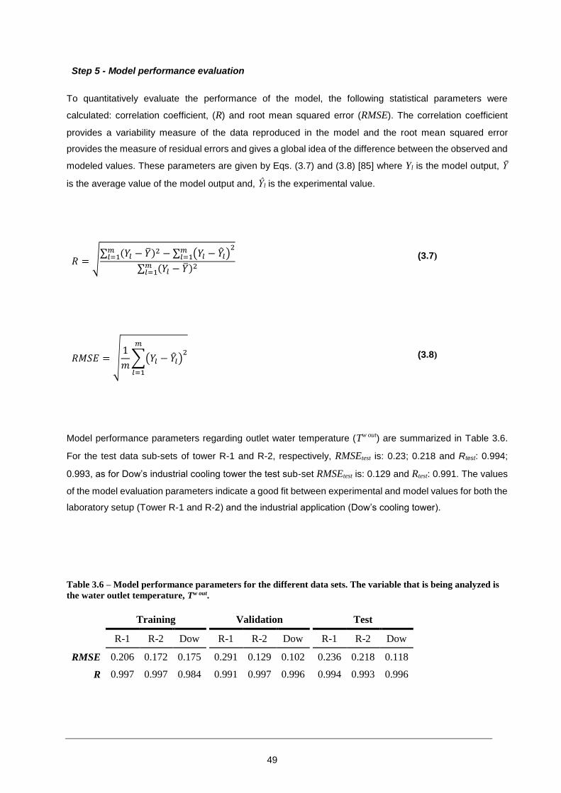
49

Step 5 - Model performance evaluation

To quantitatively evaluate the performance of the model, the following statistical parameters were

calculated: correlation coefficient, (R) and root mean squared error (RMSE). The correlation coefficient

provides a variability measure of the data reproduced in the model and the root mean squared error

provides the measure of residual errors and gives a global idea of the difference between the observed and

modeled values. These parameters are given by Eqs. (3.7) and (3.8) [85] where Yl is the model output, Ȳ

is the average value of the model output and, Ŷl is the experimental value.

𝑅 = √∑ (𝑌𝑙 − �̅�)2𝑚

𝑙=1 − ∑ (𝑌𝑙 − �̂�𝑙)2𝑚

𝑙=1

∑ (𝑌𝑙 − �̅�)2𝑚𝑙=1

(3.7)

𝑅𝑀𝑆𝐸 = √1

𝑚∑(𝑌𝑙 − �̂�𝑙)

2𝑚

𝑙=1

(3.8)

Model performance parameters regarding outlet water temperature (Tw out) are summarized in Table 3.6.

For the test data sub-sets of tower R-1 and R-2, respectively, RMSEtest is: 0.23; 0.218 and Rtest: 0.994;

0.993, as for Dow’s industrial cooling tower the test sub-set RMSEtest is: 0.129 and Rtest: 0.991. The values

of the model evaluation parameters indicate a good fit between experimental and model values for both the

laboratory setup (Tower R-1 and R-2) and the industrial application (Dow’s cooling tower).

Table 3.6 – Model performance parameters for the different data sets. The variable that is being analyzed is

the water outlet temperature, Tw out.

Training

Validation

Test

R-1 R-2 Dow

R-1 R-2 Dow

R-1 R-2 Dow

RMSE 0.206 0.172 0.175

0.291 0.129 0.102

0.236 0.218 0.118

R 0.997 0.997 0.984

0.991 0.997 0.996

0.994 0.993 0.996

50

Although the model was trained using only water outlet temperatures the model performance parameters

regarding air outlet temperatures (Ta out) in tower R-1 and R-2 also indicate an acceptable fit between model

predictions and experimental values: RMSEtest = 0.349; Rtest = 0.988 for tower R1 and RMSEtest = 0.130;

Rtest = 0.997 for tower R-2. In an industrial context air outlet temperature is not a critical variable to be

controlled, therefore these values are not available for Dow’s case study and the comparison between

model and experimental air outlet temperatures was not possible to accomplish.

All predicted values are within a margin of ±2 % from the experimental values for water outlet temperatures

and ±3 % for air outlet temperatures (tower R-1 and R-2).

3.1.3 Cooling system thermodynamic model

The hydraulic performance of the network is evaluated with the developed hydraulic model, i.e., the cooling

water flow rates flowing through the heat exchangers were determined. On the other hand, with the ASPEN

PLUS thermodynamic model, the temperature on each point of the network was evaluated.

Figure 3.14 shows the cooling water system as a block diagram. The cooling water system is composed by

a combination of the cooling water network, where heat is transferred from the process to the cooling water,

and the cooling tower, where heat is transferred from the cooling water to ambient air. By combining each

heat exchanger duty and cooling water flow with the cooling tower model, it is possible to establish an

accurate model that describes the plant cooling water system. The thermodynamic model of the cooling

water system was developed with the ASPEN PLUS simulator. The global property method used in the

flowsheet was set to IDEAL and is applied throughout.

51

Figure 3.14 – Block diagram of the cooling water system model.

HO

2H

O3

HO

1H

O5

HO

6H

O4

HO

8H

O9

HO

7H

O1

0H

On

HI1

HI2

HI3

HI4

HI5

HI6

HI7

HI8

HI9

HIn

HI1

0

H1

0LO

P

H1

0LO

PI

H1

0LO

PO

CA

LCST

RM

PU

MP

SPLT

MIX

SPLT

10

MIX

10

H2

H1

H4

H3

H6

H5

H8

H7

H9

Hn

H1

0

PU

MP

OU

T

CTW

RA

DFR

AC

WA

TRET

AIR

IN

MA

KEU

P

WO

UT

PU

RG

E

WA

TSU

P

AIR

OU

T

MIX

MU

PSP

LTP

UR

G

WO

UT2

WA

TSU

P2

52

Cooling tower model

The graphical display of the cooling tower (CTW) model implemented in ASPEN PLUS is shown in Figure

3.15. A detailed description of the model was previously described in Section 3.1.2 The Cooling Tower

Model and consists on a RADFRAC block without reboiler and condenser, two equilibrium stages with the

calculation type set as ‘Equilibrium’. At the bottom stage “dry” air (AIRIN) enters ‘On-stage’ and cooled

water (WOUT) exits; at the top stage “humid” air (AIROUT) exits and hot water (WATRET) enters ‘Above-

Stage’. The Murphree efficiency of the top stage is Effw,1M = 0.96 and the Murphree efficiency of the bottom

stage is Effw,2M = 0.70.

The intermediary stream (WOUT2) that resulted from mixing the cooled outlet water stream (WOUT) with

the makeup stream (MAKEUP) enters in a SPLIT block where it is divided into the stream that feeds the

cooling water network (WATSUP) and a purge stream (PURGE). The purge flow is set within the SPLIT

block to 5 m3/h.

The cooling water system is semi-closed system in terms of mass balance since the majority of the flow

circulates cyclically. However, there are losses during the process: by evaporation in the cooling tower and

because of the purge flow that is required to maintain an acceptable quality of the cooling water. To account

these losses, a makeup of fresh water is required. So, the cooled outlet water stream (WOUT) is mixed

with the makeup stream (MAKEUP) in a MIXER block (MIXMUP), resulting in an intermediary stream

(WOUT2).

The “Design Spec” tool of the ASPEN PLUS was used for determining the flow of fresh makeup. The mass

flow of the supply (WATSUP) and return (WATRET) streams were as defined as variables. Then, it was

defined that the mass flow of WATSUP should be equal to the one of WATRET by varying the MAKEUP

mass flow.

Although the purge flow rate of 5 m3/h is relatively small when compared to the total flow rate, 5678 m3/h,

it would make sense that the purge was taken ahead of the makeup so that the purge would be more

effective. However, the makeup takes place in the cooling tower basin whereas the purge is taken from the

outlet stream.

53

Figure 3.15 – Detail of the cooling tower thermodynamic model implemented in ASPEN PLUS.

Cooling water network

Each heat exchanger in the network was described by a HEATER block. The input variables of each block

were pressure drop and heat duty. Heat duty of each heat exchanger was based on design values.

In Figure 3.16,the graphical display of the cooling water network model implemented in ASPEN PLUS is

shown. The water living the cooling tower (WATSUP2) goes through a cooling water pump (PUMP) where

it is pressurized from 0 barg to 5.3 barg, increasing 0.1 C in the compression process. The outlet stream of

the PUMP block (PUMPOUT) then enters a SPLIT block (SPLT), which can be interpreted as the cooling

water supply header, dividing the inlet stream into each individual heat exchanger flow (HI1, HI2,…, HIn).

The specific flow of each heat exchanger was previously determined with the hydraulic model of the cooling

water network, as described above. Cooling water then enters each heat exchanger (H1, H2,…,Hn), where

it is heated by the process stream. The heat duty of each exchanger and pressure drop of each heat

exchanger are inputs of the each HEATER block. Since cooling water is a liquid stream and no flash is

involved, the pressure drop defined in the heat exchangers has little influence on the outlet stream

conditions in regard to temperature and physical state so, an arbitrary value of 0.8 barg for the pressure

drop was assumed. The outlet streams (HO1, HO2,…, HOn) are combined in a MIXER block (MIX), which

can be interpreted as the cooling water return header. The combined outlet stream (WATRET) follows to

the cooling water to complete the cooling water system cycle. The IDEAL property method was used to

simulate every block.

CTW

RADFRAC

WATRET

AIRIN

MAKEUP

WOUT

PURGE

WATSUP

AIROUT

From CoolingWater Network

To CoolingWater Network

MIXMUP SPLTPURG

WOUT2

54

Due to process requirements, there were some heat exchangers where the inlet temperature had to be

higher than the one supplied by the cooling water distribution network. In these cases, a recycling loop was

used such as shown in Figure 3.16. The inlet stream of the cooler (H10LOPI) was fed into the heat

exchanger (H10) and heated by a given duty. The outlet stream (H10LOPO) then entered in a SPLIT block

(SPLT10) where it was divided into two streams: one was recycled (H10LOP) and the other (H10O) followed

to the return header. The recycled stream (H10LOP) was then mixed with “fresh” cooling water (H10) in a

MIXER block (MIX10), generating a “warm” stream and thus completing the loop.

The known variables regarding the heat exchangers with recycling loops were the heat exchanger’s flow

rate and temperature of the inlet stream (H10LOP) and the exchanger’s (H10) heat duty. The unknown

variables were the recycled stream (H10LOP) flow rate and “fresh” water flow rate. To determine the flow

rate of “fresh” cooling water a ‘Design Spec’ was used. The temperature of the “warm” inlet temperature of

the cooler (H10LOPI) was as defined as variable. Then, it was defined that the temperature of the heat

exchanger inlet stream (H10LOPI) should be equal to a given temperature by varying the “fresh” cooling

water (H10) mass flow rate.

The recycled stream (H10LOP) flow rate was determined using a CALCULATOR block. This block allowed

some Fortran code to be implemented defining the loop mass balance. By declaring the heat exchanger’s

inlet flow rate (H10LOPI), which is a known variable, and stating that the recycled mass flow rate is equaled

to the inlet flow rate minus the “fresh” water flow rate ( Eq. (3.9)), which was manipulated by the

abovementioned ‘Design Spec’, it was possible to calculate in the recycle stream flow rate.

𝐻10𝐿𝑂𝑃 [𝑘𝑔

ℎ] = 𝐻10𝐿𝑂𝑃𝐼 [

𝑘𝑔

ℎ] − 𝐻𝐼10 [

𝑘𝑔

ℎ]

(3.9)

The SPLIT block determines the flow of one of the block’s outlet streams based on the difference between

the inlet stream and the sum of the other stream flow rates. So, to simplify the cooling water network model

by avoiding the necessity of varying the cooling water inlet flow (WATSUP2) to the SPLIT block, an auxiliary

stream was applied (CALCSTRM). This stream’s mass flow rate is the difference between the inlet cooling

water flow rate to the SPLIT block (WATSUP2) and the total sum of the mass flow rates of the streams

feeding the heat exchangers (HI1, HI2,…, HIn). Therefore, by assigning a sufficiently large mass flow rate

to the WATSUP2 stream, the SPLIT block was always in mass balance despite variations in the network

mass balance.

To work around the fact that cyclic systems are harder to converge in ASPEN PLUS and the cooling water

system is a semi-closed structure the WATSUP and the WATSUP2 streams are not connected to each

other (as seen in Figure 3.14). To ensure that both streams were at the same temperature a CALCULATOR

block was implemented. The WATSUP and WATSUP2 temperatures were declared as ‘Tear’ variables with

the Fortran statements declaring that the WATSUP2 temperature was equal to the WATSUP temperature.

In the CALCULATOR block ‘Sequence’ options, it was defined that it should be executed after the

SPLTPURG block.

55

Figure 3.16 – Detail of the cooling water network thermodynamic model implemented in ASPEN PLUS.

In Figure 3.17, the cooling water system flowsheet implemented in ASPEN PLUS is presented. There are

a total of 37 heat exchangers in the network of which 4 are integrated in loop and fed with “warm” water.

Figure 3.17 – ASPEN PLUS model of cooling water network integrated with cooling tower.

WATSUP2

From CoolingTower

To CoolingTower

HO2

WATRET

HO3HO1 HO5 HO6HO4 HO8 HO9HO7 HO10 HOn

HI1 HI2 HI3 HI4 HI5 HI6 HI7 HI8 HI9 HIn

HI10

H10LOP

H10LOPI H10LOPO

CALCSTRM

PUMPSPLT

MIX

SPLT10MIX10

H2H1 H4H3 H6H5 H8H7 H9 Hn

H10

PUMPOUT

56

3.1.4 Evaluation of the performance of the cooling water system

Some cooling water parameters determined using the thermodynamic model for a 21 C air wet-bulb

temperature are presented in Table 3.7.

The thermodynamic model showed that the temperature range between the supply and overall return

streams is approximately 6 C for the Dow’s cooling water network. The fact that the range value is not an

exact figure results from the fact that it slightly varies with the air wet-bulb temperature. This is due to the

presence of loops in the cooling water network that influences the cooling water circulating flow. For

instance, since the cooling duty is constant, when the cooling water supply temperature decreases due to

a lower air wet-bulb temperature, the required “fresh” water flow rate to each loop will also decrease,

therefore reducing the cooling water overall circulating flow rate and therefore increasing the range.

However, since the heat duty of the heat exchanger with loop corresponds to only 5% of the total heat duty,

the range variation is not significant, varying 0.08 C with a 3 C variation in the air wet-bulb temperature.

Table 3.7 – Dow’s cooling water network parameters for a 21 C air wet-bulb temperature.

Range (Treturn – Tsupply) 6 C

Cooling duty of the

network

37.6 MW

Circulating cooling

water flow rate

5678 t/h

Water lost due to

evaporation

30.6 t/h

Figure 3.18 shows the results of performing a sensitivity analysis using the thermodynamic model of the

cooling system, where the cooling water network supply temperature is calculated by varying air wet-bulb

temperature for different cooling ranges are shown.

The maximum design cooling water supply temperature for the process is set to 26 C. Taking the results

shown in Figure 3.18 into consideration, which corresponds to a 21 C air wet-bulb temperature i.e. if the

air wet-bulb temperatures rises above 21 C the cooling water supply temperature will be above design.

To work within design boundaries, it is necessary to reduce the cooling water range (decrease cooling

duty) and therefore reduce production rate.

57

Figure 3.18 – Cooling water supply temperature vs Air wet bulb temperature for the Dow’s cooling tower.

Given the limit air wet-bulb temperature of 21 C, it is now relevant to determine how the cooling water

system design is adequate to the environmental conditions at the Estarreja site.

A cooling tower with lower capacity implies that the plant rate is limited by the cooling tower for longer

periods whereas a cooling tower with high capacity might mean that the cooling tower is overdesigned

and a higher capital investment is required.

Given a set of historic weather data, it is possible to determine how long throughout the year was the air

wet-bulb temperature above a given temperature. Combining this information with the limit value of the

wet-bulb temperature of cooling water system, the time during which the cooling tower would be limiting

the production rate can be determined.

Records regarding weather data at the Dow’s Estarreja MDI plant were not available. Therefore, to estimate

the wet-bulb temperature’s annual frequency, data was retrieved from the Ovar weather station, which is

approximately 15 km away from the plant, corresponding to the whole of year 2010 [84].

Figure 3.19 displays the frequency of occurrence of different wet-bulb temperatures is presented. The figure

can be used to answer the following question: During 2010, what was the percentage of the year during

which the temperature was higher than a given wet-bulb temperature? For example, the wet-bulb

temperature was higher than 13.8 C during approximately half of the year.

23.5

24

24.5

25

25.5

26

26.5

27

27.5

18 19 20 21 22 23

Co

olin

g W

ater

Su

pp

ly t

emp

erat

ure

(C

)

Air Wet-Bulb Temperature (C)

Range = 6.5 C

Range = 6.0 C

Range = 5.5 C

58

At maximum plant rate, the abovementioned cooling tower maximum outlet temperature was set to be

26 C and to achieve this temperature, the ambient air wet-bulb temperature must lower than 21 C. It is

possible to observe in Figure 3.19 that during 2010 the wet-bulb temperature was above 21 C, which is

the temperature above which the cooling tower limits the production rate, during approximately 4.5% of

the year. This represents 394 hours of disrupted production rate due to cooling tower limitations.

Figure 3.19 – Estimated wet-bulb temperature frequency of occurrence in 2010 at Dow’s Estarreja MDI plant.

59

3.2 Steam system analysis

3.2.1 Steam generator

Steam is one of the most widely used media for conveying thermal energy within several industries. Some

reasons that make steam so attractive for utilization in a process is the fact that water is readily available,

relatively inexpensive, non-toxic and environmentally safe. In its vapor form, it is a safe and efficient energy

carrier. Steam has a high energy density and can hold much more potential energy as an equivalent mass

of liquid water and since the heat transfer coefficient of steam is so high, the required heat transfer area is

relatively small. This enables the use of heat exchangers with smaller heat transfer areas, which are

cheaper and with a lower footprint.

Steam is often generated in one or more boilers and then distributed to the various consumption points

through a piping network. This centralized arrangement means that the boiler is an obvious target for

optimization efforts that promote the improvement of its efficiency.

The performance test code for fired steam generators from the American Society of Mechanical Engineers

[86] describes two different methods for determining the boiler efficiency: the direct and the indirect method.

The direct method, also known as the input-output method, is essentially the ratio between the energy

that is transferred to the steam and the total energy supplied by the fuel. Eq. (3.10) describes the boiler

efficiency calculated through the direct method, ηdm, where Qstm is the energy transferred to the steam and

Qfuel is the total energy contained in the fuel fed to the boiler.

𝜂𝑑𝑚 =𝑄𝑠𝑡𝑚

𝑄𝑓𝑢𝑒𝑙

(3.10)

On the other hand, the indirect method, Eq. (3.11), computes boiler efficiency, ηim, based on the total

energy contained in the fuel fed to the boiler subtracted by the boiler losses, where Xlosses is the ratio

between Qfuel and the total boiler losses.

𝜂𝑖𝑚 =𝑄𝑓𝑢𝑒𝑙 − 𝑄𝑓𝑢𝑒𝑙 ∙ 𝑋𝑙𝑜𝑠𝑠𝑒𝑠


= 1 − 𝑋𝑙𝑜𝑠𝑠𝑒𝑠

(3.11)

For determining boiler efficiency using the direct method it is only necessary to quantify the inlet fuel

enthalpy and the enthalpy transferred to the steam. The uncertainty of the direct method is directly

proportional to the uncertainty of measurement of the feed water/steam flow rate, feed water and steam

specific enthalpy, fuel flow rate and fuel heating value. As for the indirect method, it does not rely on the

flow rate measurement of fuel and feed water/steam but instead on the determination of boiler losses

through a detailed energy balance.

So, while boiler efficiency is simpler to compute using the direct method, the indirect method is the

preferred approach to determine boiler efficiency [86]. This is because the direct method requires very

60

sensitive flowmeters to accurately determine steam and fuel flow, which are not commonly found in

industrial boilers, whereas in the indirect method measurement errors impact only on the losses rather

than all the total energy.

As an example, if the real boiler efficiency calculated through the direct method is considered as being ηdm

real and ηdm dev the boiler efficiency deviated by an error, if there is an error in steam flow measurement of

1%, Eq. (3.12) , assuming a 90% boiler efficiency this will impact on the calculated efficiency ± 0.9%.

𝜂𝑑𝑚 𝑑𝑒𝑣 =𝑄𝑠𝑡𝑚 𝑟𝑒𝑎𝑙 ∙ (1 ∓ 1%)


= 𝜂𝑑𝑚 𝑟𝑒𝑎𝑙 ∙ (1 ∓ 1%)

(3.12)

If ηdm real = 90%

Then,

𝜂𝑑𝑚 𝑑𝑒𝑣 = 𝜂𝑑𝑚 𝑟𝑒𝑎𝑙 ∓ 0.9%

(3.13)

As for the indirect method,

𝜂𝑖𝑚 𝑑𝑒𝑣 =𝑄𝑓𝑢𝑒𝑙 − 𝑄𝑓𝑢𝑒𝑙 ∙ 𝑋𝑙𝑜𝑠𝑠𝑒𝑠 ∙ (1 ∓ 1%)


= 1 − 𝑋𝑙𝑜𝑠𝑠𝑒𝑠 ∙ (1 ∓ 1%)

𝜂𝑖𝑚 𝑑𝑒𝑣 = 1 − 𝑋𝑙𝑜𝑠𝑠𝑒𝑠 ∓ 𝑋𝑙𝑜𝑠𝑠𝑒𝑠 ∙ 1% = 𝜂𝑖𝑚 𝑟𝑒𝑎𝑙 ∓ 𝑋𝑙𝑜𝑠𝑠𝑒𝑠 ∙ 1%

(3.14)

If Xlosses = 10%

𝜂𝑖𝑚 𝑑𝑒𝑣 = 𝜂𝑖𝑚 𝑟𝑒𝑎𝑙 ∓ 0.1%

(3.15)

Figure 3.20 shows a diagram of the energy balance of the steam generator where the input and output heat

streams are shown as well as a list of the potential losses in the boiler. A detailed description of the

methodology used to calculate each parameter of the energy balance is well described elsewhere in the

American Society of Mechanical Engineers (ASME) performance test code for fired steam generators [86]

and therefore will not be detailed here.

61

Figure 3.20 – Energy balance of steam generator envelope.

The boiler efficiency calculation method described on ASME manual is based on the fuel high heat value

(HHV) and therefore takes into account air moisture and losses due to moisture from burning hydrogen.

The reference state is liquid water so, unless the boiler system has a recovery unit that allows the

condensation of water present in the flue gas, boiler efficiency based on HHV is significantly lower than the

efficiency based on the lower heating value (LHV).

The process variables and assumed parameters considered for the boiler efficiency calculation are stated

in Table 3.8. Although the indirect method does not calculate efficiency directly from fuel flow rates, it does

require entry of flowrates to determine relative fractions of fuels and losses due to surface radiation.

Carbon monoxide is not measured online, so the value stated in Table 3.8 is assumed that carbon monoxide

concentration in the flue gas is 80% of the upper limit imposed by the environmental permit [87] and is

considered to be constant for all three boilers. Additionally, since the boilers use natural gas as fuel,

unburned carbon is considered to be negligible.

Boiler efficiency was calculated assuming the fuel composition detailed in Table 3.9. The natural gas

property data was provided by the natural gas supplier regarding the average composition during a one

month period. The main constituent of the fuel stream is methane, with a molar fraction of 89.9%, followed

by ethane, with a molar fraction of 6.79%. The rest of the fuel constituents are inert gases, totalling 0.92%,

and other longer chain hydrocarbons corresponding to 2.38%.

62

Table 3.8 – Model parameters for calculating boiler efficiency using the indirect method.

Inlet combustion air temperature

Online measurement

Exhaust gas temperature

Online measurement

Fuel flow rate Online measurement

Ambient temperature 23 oC

Air relative humidity 80%

Boiler skin area 184 m2

Boiler skin

temperature

50 ºC

Carbon monoxide in

stack

400 mg/Nm3

Unburned fuel as total

organic carbon

(Neglectable)

Table 3.9 – Average fuel composition during April 2011 (composition provided by fuel supplier) and high and

low heating values [88].

Component HHV

(kJ.kg-1) LHV

(kJ.kg-1) Formula Mol. Fraction

Nitrogen - - N2 0.32%

Carbon

Dioxide - - CO2 0.60%

Methane 37 620 33 866 CH4 89.90%

Ethane 65 904 60 285 C2H6 6.79%

Propane 93 799 86 316 C3H8 1.90%

n-Butane 121 543 111 874 C4H10 0.21%

IsoButane 121 192 111 798 C4H10 0.27%

TOTAL 48 240 43 560 100 %

Figure 3.21 to Figure 3.23 show the variation of boiler efficiency based on LHV with stack temperature and

excess oxygen in exhaust gas for different fuel flows. A higher stack temperature means that less energy

is being recovered from the flue gas to generate steam and therefore is being lost to the environment. On

the other hand, higher excess oxygen in stack implies that the flow of combustion air admitted to the boiler

is too high, meaning that energy is being lost by heating up an unnecessary quantity of combustion air. As

mentioned earlier, the indirect method does not calculate efficiency directly from fuel flow rates. However,

since it is assumed that the radiation losses are constant and independent from the fuel flow rate, specific

radiation losses will vary inversely to fuel flow rate, i.e., radiation losses per “unit” of fuel will decrease for

higher rates and decrease for lower rates, thus impacting on the overall boiler efficiency.

63

Figure 3.21 – Boiler efficiency based on LHV vs. stack temperature calculated using the indirect method for

different values of oxygen content in stack. Fuel flow = 500 kg/h



91.00

92.00

93.00

94.00

95.00

96.00

100 120 140 160 180 200 220

Bo

iler

Eff

icie

ncy

(% )

Stack Temperature (oC)

2.5%

3.0%

3.5%

4.0%

4.5%

5.0%

Excess O2 in

stack

91.00

92.00

93.00

94.00

95.00

96.00

100 120 140 160 180 200 220

Bo

iler

Eff

icie

ncy

(% )


2.5%

3.0%

3.5%

4.0%

4.5%

5.0%

Excess O2 in

stack

64



Plots in Figure 3.21 to Figure 3.23, showing the relation between stack temperature, excess oxygen in stack

and boiler efficiency for different fuel loads are useful tools for assessing boiler efficiency at a given

operating point.

By observing Figure 3.21 to Figure 3.23, some remarks can also be taken: While keeping the same stack

temperature, lowering oxygen content in stack does not have an effect on boiler efficiency by the same

magnitude, i.e. lowering oxygen content by 1% does necessarily means that boiler efficiency will increase

by 1%.

Figure 3.24 to Figure 3.26 illustrate the comparison between the results obtained when using the direct

and the indirect method. The comparison is done for the three boilers in the Estarreja plant.

It is possible to observe from Figure 3.24 to Figure 3.26 that boiler efficiency calculated with the direct

method is much more disperse than when using the indirect method. The reason for the evident difference

between both methods is explained by the different approaches in the abovementioned calculation

methods. While the indirect method takes into account more reliable measurements, such as fuel flow rates,

stack temperatures and flue gas oxygen contents, the direct method relies on the correct measurement of

steam generated by the boiler, which is known to be a difficult medium to retrieve a precise flow rate

quantification.

91.00

92.00

93.00

94.00

95.00

96.00

100 120 140 160 180 200 220

Bo

iler

Eff

icie

ncy

(% )


2.5%

3.0%

3.0%

4.0%

4.5%

5.0%

Excess O2 in

stack

65

(a) (b)

Figure 3.24 – B4001 boiler efficiency using the input-output method (●) and the direct method (×).

(a) (b)


66

(a) (b)


A polynomial trend line was fitted to the data regarding the boiler efficiency and natural gas flow for all

three boilers. The quadratic equation that was adjusted to the data shown in Figure 3.24 to Figure 3.26

regarding the relation between fuel flow (Qfuel) and boiler efficiency calculated with the indirect method

(ηim) is given by Equation (3.16).

𝜂𝑖𝑚 (%) = 𝑎 × 𝑄𝑓𝑢𝑒𝑙2 + 𝑏 × 𝑄𝑓𝑢𝑒𝑙 + 𝑐

(3.16)

The adjusted parameters for each boiler used in Equation (3.16) are shown in Table 3.10. Although the

squared correlation coefficient (R2) is very low for all three boilers: 0.14, 0.03 and 0.06 for B4001, B4002

and B4003, respectively, the equations are still useful for estimating the average boiler efficiency given

any given fuel flow.

Table 3.10 – Parameters for describing the relation between boiler efficiency and fuel flow, described by

Equation (3.16), regarding the three boilers.

a b c

B4001 -6.96×10-6 1.15×10-2 89.2

B4002 -4.03×10-6 5.14×10-3 92.2

B4003 -5.05×10-6 7.95×10-3 90.1

Figure 3.27 shows the relation between efficiency, based on LHV, and boiler load provided by the vendor

[89]. The plot shows this relation for different boilers, characterized by their efficiencies when operating at

100% load. In the case of the Estarreja MDI plant, the vendor states that efficiency at 100% load is 91%,

meaning that the maximum achievable efficiency is approximately 91.5% when operating at 80% of

maximum capacity. However, the data provided by the vendor was based upon the assumption that the

67

boiler would operate with fuel oil. Additionally, excess oxygen content and stack temperature is not

specified.

Figure 3.27 – Efficiency curves for different boilers provided by the vendor [89].

When comparing the calculated efficiency for each boiler with the data provided by the vendor, it is possible

to verify that the calculated efficiency for each boiler is generally higher, usually above 93%. This can be

due to the fact that natural gas is a “cleaner” fuel and does not produce as much soot as fuel oil, rendering

a more efficient burn with less heat exchanger fouling. Also, vendor data does specify oxygen content in

stack, meaning that the efficiency curves provided by the vendor might be assuming a higher oxygen

content in stack than the one that the boilers are normally operated.

By determining each boiler efficiency, it is then possible to calculate the steam produced by each boiler

based on the fuel flow.

Boiler efficiency, η, the ratio between the energy transferred to the steam and the energy input is calculated

using Eq. (3.17). This efficiency is referred to the fuel low heat value (LHV).

83

84

85

86

87

88

89

90

91

92

93

0 20 40 60 80 100

Effi

cie

ncy

(% )

Boiler Load (% of maximum capacity)

92%

91%

90%

89%

88%

87%

86%

85%

92 %

91 %

90 %

89 %

88 %

87 %

86 %

85 %

Eff

icie

ncy

(%

)

Boiler load (% of maximum capacity)

68

𝜂 =𝑄 ∙ (𝐻𝑉 − 𝐻𝐵𝐹𝑊)

𝐵 ∙ 𝐿𝐻𝑉× 100

(3.17)

Where, Q is the steam load (kg/h), Hv and HBFW are the steam and boiler feed water enthalpy (kJ/kg), B is

the fuel load (kg/h) and LHV is the low heat value of the fuel.

Based on the boilers behavior described by the parameters stated in Table 3.10, different operating

methods were analyzed: Either steam production was equally distributed across the three boilers or the

load was distributed so that fuel consumption was minimized.

For finding the load distribution that rendered the minimum fuel consumption the Solver tool available in

Microsoft Excel 2013 [90] was used.

The chosen method for solving the optimization problem was the GRG nonlinear method, but since the

problem in highly non-linear, a global minimum cannot be guaranteed. However, to ensure that the solver

provided the “best” solution, constraints regarding minimum (Q > 0 kg/h) and maximum (Q < 25000 kg/h)

boiler steam production were considered. Additionally, several initialization points, within the stated boiler

limits, were tested.

Considering an equal steam load distribution scheme, where each boiler has the same steam production,

fuel consumption for various steam production levels is stated in Table 3.11. In Table 3.12, the same

information is shown but instead regarding an optimal distribution scheme, where the fuel consumption is

minimized. Table 3.13 presents the comparison between both schemes in regard to fuel consumption.

Table 3.11 –Estimated fuel consumption for different steam production levels assuming an equal steam load

distribution.

Equal load distribution

Fuel Consumption (kg/h) Steam Production (kg/h)

B4001 B4002 B4003 B4001 B4002 B4003 Total

398 394 398 6667 6667 6667 20000

494 491 496 8333 8333 8333 25000

591 589 593 10000 10000 10000 30000

687 687 691 11667 11667 11667 35000

785 786 789 13333 13333 13333 40000

883 886 889 15000 15000 15000 45000

69

Table 3.12 – Estimated fuel consumption for different steam production levels assuming an optimal steam

load distribution.

Optimal load distribution

Fuel Consumption (kg/h) Steam Production (kg/h)

B4001 B4002 B4003 B4001 B4002 B4003 Total

779 400 0 13233 6767 0 20000

736 737 0 12493 12507 0 25000

935 833 0 15875 14125 0 30000

807 578 680 13707 9818 11475 35000

811 774 775 13780 13131 13090 40000

876 859 922 14891 14545 15565 45000

Table 3.13 – Comparison between total fuel consumption regarding equal and optimal load distribution

schemes. Improvement in fuel consumption of the optimal load distribution relatively to the equal load

distribution scheme.

Equal load distribution

Optimal load distribution

Total Steam Production (kg/h)

Total Fuel

Consumption (kg/h)

Total Fuel

Consumption (kg/h)

Fuel

Consumption Reduction

20000 1190 1178 -0.94% 25000 1482 1475 -0.60% 30000 1773 1768 -0.28% 35000 2066 2065 -0.05% 40000 2360 2360 -0.01% 45000 2657 2657 0.00%

Taking into account the comparison between fuel consumption of both load distribution schemes stated in

Table 3.13, it is possible to observe that the improvement in fuel consumption is higher for lower steam

production rates and decreases as steam production rate increases, reaching a negligible improvement

margin for higher rates.

The results lead to the conclusion that, in this specific case, distributing the load equally across the three

boilers is in fact a good option in regard to fuel efficiency. Nonetheless, the described methodology is useful

for accessing boiler performance and providing an optimization strategy for distributing boiler load, being

especially useful in cases where boilers have higher efficiency discrepancies.

3.2.2 Steam network

Since the centralized steam production is often the preferred arrangement for industrial applications, it is

then essential to have an efficient steam distribution network that delivers steam to the various consumption

70

points. Furthermore, it is essential to have a clear understating of the steam network when assessing

process modifications that involve the usage of steam as they impact on the overall balance of the network.

The purpose of producing steam in Estarreja MDI plant is solely for heating process steams. The plant uses

steam at two different grades: The abovementioned steam generation system produces high pressure (HP)

steam, at 22 barg and 275 C. Additionally, low pressure (LP) steam, at 3.8 barg and 151 C is also used in

the plant.

The steam system can be described as follows: HP steam is produced in three boilers that use natural gas

as fuel, which is then distributed to the HP steam consumers. The generated HP condensates are fed into

a flash drum, where LP steam is generated. When pressure in the LP steam header drops below a given

set-point, a pressure control valve lets down HP steam to rise the pressure in the header, whereas when

the header pressure increases, LP steam is vented to atmosphere. Some LP steam is directly injected into

the process while the remaining is distributed to LP steam consumers. The resulting LP condensates, then

go to a flash drum where they depressurize to atmospheric pressure. The condensates from the

atmospheric flash drum together with the condensates from the LP flash drum, fresh demineralized water

and a small stream of LP steam are fed into a deaerator which is at 2.1 barg to remove non-condensable

gases and therefore prevent corrosion issues. Finally, the system is closed when the condensates are fed

into the boiler through the boiler feed pumps.

A schematic view of the steam system showing the main branches of the network is presented in Figure

3.28. LP steam is vented to atmosphere when the high pressure control valve in the LP steam header is

open. However, since it is normally closed, was not depicted in Figure 3.28.

Figure 3.28 – Steam network block diagram.

LP consumers

HP consumers

Deaerator

Direct Injection

BoilerBlowdown

Make-up water

To Atm

Condensate export

LPFlash Drum

AtmFlash Drum

let down

71

3.2.3 Steam system thermodynamic model

The ASPEN PLUS thermodynamic model allows the determination of the steam and condensate flow rates

and temperature on each point of the network. With this information, it is possible to build the process flow

diagram (PFD). The global property method used in the flowsheet was set to STEAMNBS, which is the

property method that is based on the steam tables developed by the National Bureau Standards in

cooperation with the National Research Council of Canada [91] and is applied throughout the steam system

model.

In Figure 3.29, the steam system is represented with a block diagram. In this diagram, the boiler, the high

pressure steam network and the low pressure steam network envelopes are highlighted. Other relevant

components include the low pressure (LPDRUM) and atmospheric (ATMDRUM) flash drums, the letdown

valve (LDVALVE), low pressure (LPPUMP) and atmospheric (ATMPUMP) condensate pumps, and the

deaerator (DEAERATOR).

72

Figure 3.29 – Block diagram of the steam system model implemented in ASPEN PLUS.

HM

IX

H2

H1

H4

H3

Hn

HI2

HI3

HI1

HI4

HIn

HSP

TLH

STM

HC

ON

D

HO

2H

O3

HO

1H

O4

HO

n

LPD

RU

M

LMIX

L2L1

L4L3

Ln

LI2

LI3

LI1

LI4

LIn

LSP

TL

LSTM

LCO

ND

LO2

LO3

LO1

LO4

LOn

ATM

DR

UM

LSP

TL

LSM

IX

LMIX

HSP

LT

LFLA

SH

LETD

WN

LSTM

1

MK

UP

ATM

CO

ND

LPC

ON

D1

ATM

CO

ND

1

LPC

ON

D

MK

UP

1

MK

UP

2

LSTM

2

HST

M2

HST

M1

HST

M3

LPP

UM

P

ATM

PU

MPB

LRP

UM

P

DEA

ERTO

R

BLW

DW

N

DR

TRV

ENT

ATM

VEN

T

CO

ND

EXP

RT

BLR

FEED

BLR

1B

LR2

MK

UP

SPLT

EXP

RTS

PLT

BO

ILER

1B

OIL

ER2

BO

ILER

SPLT

DR

TRO

UTD

RTR

OU

T1

Bo

iler

HP

Ste

am

Net

wo

rk

LP S

tea

mN

etw

ork

LDV

ALV

E

HA

UX

LAU

X

73

Boiler

The boiler envelope shown in Figure 3.30 consists of three blocks. The first HEATER block (BOILER1)

simulates the liquid phase in the boiler, where the condensates are heated up to the specified outlet

conditions, 22 barg and vapor fraction = 0. With a SPLIT block (BOILERSPLT), to avoid over-concentrating

scaling and corrosive components in the boiler, the stream leaving the heat exchanger is split to generate

a blowdown stream of 500 kg/h (BLWDOWN) that is sent to waste water treatment. The BLR2 stream then

follows to the second heat exchanger (BOILER2), where the outlet conditions are specified as being 22 barg

and 285 C.

Figure 3.30 – Boiler envelope in ASPEN PLUS.

HP steam letdown to LP steam

LP steam is mainly generated by the flash of HP condensates in the LP flash drum. However, to meet the

demand and keep the pressure in the LP steam header, a letdown valve is responsible for generating LP

steam from HP steam.

In Figure 3.31, the HP steam produced in the boiler (HSTM1) is divided in a SPLIT block (HSPLT) to

generate the stream that is fed to the HP steam network (HSTM2) and the stream that is used to produce

LP steam (HSTM3) in the letdown valve (LDVALVE).

LP steam (LSMIX) is generated by mixing both the steam from the LP flash drum (LFLASH) and the HP

steam letdown (LETDWN) in the MIXER block (LMIX). The letdown valve is set in ASPEN PLUS as a

VALVE block where the outlet pressure was specified as being 3.8 barg.

HSTM1

BLWDWN

BLRFEEDBLR1BLR2

BOILER1BOILER2 BOILERSPLT

BoilerFrom Dearator

To HP network & Let down valve

74

Figure 3.31 – HP and LP steam generation in ASPEN PLUS.

HP steam network

The HP steam network consists in a set of heat exchangers, fed from a distribution network arranged in

parallel, i.e., steam or condensate passes only once through each heat exchanger.

In Figure 3.32, the HP steam network diagram is shown. Steam generated in the boiler (previously split in

HSPLT block, vide Figure 3.31) is fed to a SPLIT block (HSPLT) that simulates the supply header and

where flow is distributed across all consumers (HI1, HI1, …, HIn). The heat exchangers (H1, H1, …, Hn)

are set as HEATER blocks where outlet pressure is set to 21.8 barg and outlet temperature to 218.1 C,

which are conditions where vapor fraction is 0. The condensate streams (HO1, HO1, …, HOn) are mixed

in a MIXER block (HMIX), which simulates the return header.

The high pressure condensate stream (HCOND) then follows to a flash drum (LPDRUM) that is set in

ASPEN PLUS as a FLASH2 block, where pressure is set to 3.8 barg and heat duty to 0 kW. The outlet

streams are LP steam (LPFLASH) and LP condensate (LPCOND1). LP steam is fed to the LP steam

network, whereas LP condensate is fed to a pump (LPPUMP), where pressure increase is set to 0.5 barg.

The resulting stream (LPCOND) then follows to the deaerator.

LSMIX

LMIX

HSPLT

LFLASH

LETDWN

HSTM2

HSTM1

HSTM3

LDVALVE

From Boiler

From LP Flash Drum

To LP Steamnetwork

To HP steamnetwork

75

Figure 3.32 – HP network in ASPEN PLUS.

LP steam network

The LP steam network configuration is similar to the HP steam network. The LP steam network is shown

in Figure 3.33.. The main differences from the HP steam network are: the network is fed with LP steam

instead of HP steam, the outlet conditions of the heat exchanger blocks are set to 3.3 barg and 145.6 C

and there are cases where steam is injected directly into de process, as in the case of stream LI4-L4-LO4.

As for the flash drum (ATMDRUM), pressure is set to 0 barg and heat duty to 0 kW with the resulting flashed

steam being vented to atmosphere (ATMVENT). To drop down the temperature in the flash drum and

therefore minimize losses, a cool makeup stream at 23 C (MKUP1) is fed to the drum. Condensates

(ATMCOND1) are fed into a pump (ATMPUMP) that rises the pressure to 4 barg and sends the

condensates (ATMCOND) to the deaerator.

HMIX

H2H1 H4H3 Hn

HI2 HI3HI1 HI4 HIn

HSPTLHSTM

HCOND

HO2 HO3HO1 HO4 HOn

LPDRUM

LFLASH

LPCOND1

HP Steam Network

HAUX

To LetdownValve

To Deaerator

From Boiler

LPPUMP

LPCOND

76

Figure 3.33 – LP network in ASPEN PLUS.

Deaerator

Figure 3.34 shows the deaerator system as implemented in ASPEN PLUS. The exact image of the

deaerator block in ASPEN PLUS is in fact similar to a flash drum as the ones shown before, however, to

have a clearer picture of the equipment a different image was used herein.The deaerator (DEAERTOR) is

responsible for collecting the condensates from the various sources, removing the non-condensables from

the system by applying steam as a scrubbing agent (LSTM2) and then venting to atmosphere (DRTVENT).

The DEAERTOR is simulated in ASPEN PLUS using a FLASH2 block, where pressure is set to 3 barg and

heat duty to 0 kW.

Condensate streams entering in the deaerator are fresh water makeup (MKUP2), condensates generated

in the LP steam flash drum (LPCOND) and condensates generated in the atmospheric flash drum

(ATMCOND). The total makeup water (MKUP) enters a SPLIT block MKUPSPLT where the flow is divided

(10% of the total makeup flow (MKUP1) goes to the atmospheric flash drum where the remaining (MKUP2)

goes to the deaerator).

A stream (DRTOUT1) then leaves the deaerator and goes to a PUMP block (BLRPUMP), where it is

pumped to 24 barg. From the outlet stream DRTOUT1, the flow is divided in a SPLIT block (EXPRTSPLT),

100 kg/h of condensates are exported to outside boundary limits (CONDEXPRT). The remaining flow

(BLRFEED) follows to the boiler to generate HP steam and therefore complete the cycle.

LMIX

L2L1 L4L3 Ln

LI2 LI3LI1 LI4 LIn

LSPTLLSTM

LCOND

LO2 LO3LO1 LOn

ATMDRUM

ATMVENT

ATMCOND1

LP Steam Network

LAUX

To Deaerator

From LSPTL

ATMPUMP

ATMCOND

LO4

MKUP1

From LSPTL

77

Figure 3.34 – Deaerator in ASPEN PLUS.

Design Specs and Calculator blocks

To calculate some of variables of the steam system, several Design Specs and Calculator blocks were

used in the ASPEN PLUS simulation.

Design specs

For each heat exchanger, the calculated net-duty of the exchanger was specified as being a variable. The

target specification for this variable was then set to the known heat duty of the exchanger by manipulating

steam flow in the HSPLT or LSPLT block, depending if the exchanger was part of the HP or LP steam

network. This Design Spec facility allowed the simulator to manipulate the inlet steam flow until the desired

heat duty was achieved.

Like the cooling water system, the steam system is a semi-closed structure in terms of mass balance. To

work around the fact that cyclic systems are harder to converge in ASPEN PLUS, the LSTM and the LSTM2

streams are not connected to each other (as seen in Figure 3.29). A Design Spec is then used to vary

LSTM flow with the objective that the LAUX stream flow is negligible, here set to 0.1 kg/h. Another Design

Spec is used to manipulate LSTM1 flow in block LSPLT so that it is equal LSTM flow.

The required steam flow to work with the deaerator is 1140 kg/h. To accomplish this, a Design Spec is used

to vary the flow of the HP stream (HSTM3), being fed to the let-down valve (LDVALVE) in block HSPLT.

The objective is to obtain a steam flow being fed to the deaerator (LSTM2) equal to 1140 kg/h.

MKUPMKUP1

MKUP2

LSTM2 BLRPUMP

DEAERTOR

DRTRVENT

CONDEXPRT

BLRFEED

MKUPSPLT

EXPRTSPLT

DRTROUT

DRTROUT1

ATMCOND LPCOND

From LP Flash Drum

From ATM Flash Drum

To ATM Flash Drum

To Boiler

From LSPLT

78

As for the HP steam network, a Design Spec is used so that HSTM flow is varied and HAUX stream flow is

negligible and equal 0.1 kg/h. Finally, a design spec is used to manipulate the makeup flow (MKUP) so that

HSTM2 flow is equal to the one of stream HSTM.

Calculator block

Since the let-down valve generates superheated steam, the mixture of the saturated steam generated in

the LP flash drum and the steam generated in the letdown valve generates steam that is slightly

superheated. Thus, the temperature of steam in stream LSTM1 is set to be equal to the one in stream

LSTM by means of a CALCULATOR block.

Model outputs

The thermodynamic model of the steam network is used to determine process conditions on each point of

the network and evaluate the overall balance of the network. Figure 3.35 shows the process flow diagram

with the mass flow on the main branches of the steam network.

This model is then used to evaluate the impact that the heat integration options have on the steam network.

Figure 3.35 – Steam network block diagram.

Taking into account the steam balance shown in Figure 3.35, there is a drive for reducing 3324 kg/h of LP

steam consumption without having to make any change in the network configuration of parameters. It is

possible however that less than predicted LP steam is generated by the let-down valve. This might be due

to steam trap malfunctions or bypasses, enabling HP steam to be let-down to the HP condensates and

consequently generating a higher quantity of flashed LP steam. In this case, LP steam would be generated

in the steam traps instead of the letdown valve. Therefore, any modification to the system aiming towards

LP consumers

HP consumers

Deaerator

46569 kg/h

43245 kg/h

6161 kg/h

3324kg/h

1140 kg/h

37084 kg/h

3644 kg/h

4701 kg/h Direct Injection

Boiler500 kg/h

Blowdown

Make-up water

237 kg/hTo Atm

589 kg/h

5112 kg/h3976 kg/h

143 kg/hTo Atm

100 kg/hCondensate

export

LPFlash Drum

AtmFlash Drum

let down

79

decreasing LP consumption should be preceded by the implementation of programs that monitor the

maintenance of the steam straps.

3.2.4 Steam cost estimation

For evaluating the economic viability of the various heat exchanger configurations, it is essential to properly

determine steam cost.

Table 3.14 shows the base parameters used to determine steam cost: Demineralized water and natural

gas price refer to 2012 price; boiler efficiency is an average value based on the analysis performed in

Section 3.2.1; process heat consumption, steam generated in boiler and demineralized water consumption

were determined by the mass and heat balances of the steam network; boiler feed water enthalpy refers to

liquid water at 22 barg and 135.2 C and steam enthalpy to superheated steam at 23 barg and 285.0 C,

with the reference state being 0 barg and 0 C [92].

For clearness sake, a variable number Xi is attributed to each parameter. In Table 3.15, this variable

numbers are employed for showing the formulas used to calculate each parameter.

Table 3.14 – Parameters for steam cost estimation

X1 Demin Water price 1.367 €/t

X2 Boiler efficiency (LHV) 93.6 %

X3 Natural Gas (LHV) price 29.4 €/MWh

X4 Process heat consumption 30.1 MW

X5 Steam generated in boiler 45.0 t/h

X6 Demin Water consumption 5.6 t/h

X7 Boiler feed water enthalpy 570.0 kJ/kg

X8 HP Steam enthalpy 2977.7 kJ/kg

Table 3.15 shows the intermediate parameters, which lead to the determination of HP steam. HP steam

cost was estimated as 0.021 €/kg or 39 €/MWh.

80

Table 3.15 – Steam cost estimation intermediate calculation parameters.

X9 =𝑋5 ∙ (𝑋8 − 𝑋7)

3600⁄

Qin to HP steam 30.1 MW

X10 =𝑋9

𝑋2⁄ − 𝑋9 Qlost boiler 2.1 MW

X11 = 𝑋9 + 𝑋10 Total Qin on NG 32.1 MW

X12 =𝑋11

1⁄ Hourly Natural gas duty = 32.1 MW.h-1

X13 = 𝑋12 ∙ 𝑋3 Cost of Natural gas 944 €/h

X14 = 𝑋1 ∙ 𝑋6 Cost of Demin H2O 8 €/h

X15 =(𝑋13 − 𝑋14)

𝑋5⁄

Cost of HP steam 21 €/te

X16 =(𝑋13 − 𝑋14)

𝑋9⁄

Cost of HP steam 39 €/MWh

81

4 Stream match methodology

Pinch analysis is an useful methodology for identifying the minimum utility targets based on the heat and

temperature availability in each range. However, in industrial contexts, there are several layout constraints

that involve particular costs when modifications are to be implemented in a new or existent network.

The common framework for applying pinch methodology is focused mainly on the energy minimization of

the heat exchanger network. Nevertheless, for industrial applications, it is often necessary to consider other

costs such as piping, special materials, process incompatibilities, etc. When designing or retrofitting a heat

exchanger network, these limitations are often bypassed by relying on heuristics and experience. Other

limitation of the basic pinch methodology is that the approach temperature is fixed for all heat exchangers

located at the pinch. However, an optimal global temperature approach does not mean that the local

temperature approach of each heat exchanger is optimal. The new stream match methodology proposed

in this chapter allows a relaxation of the approach temperature of the heat exchangers located at the pinch,

therefore further optimizing the designs.

An important concept that pinch technology defines in the one that gives the name to the methodology itself:

The ‘Process pinch’. This concept is important because it defines the temperature at which the process is

most constrained in terms of temperature gradient [93]. The new stream match methodology uses this

concept to apply different rules depending on whether the stream is above, bellow or crossing the pinch.

Although pinch methodology allows the consideration of forbidden matches to determine hot and cold

energy targets, it is not straightforward how to build the network taking into account the forbidden matches

as well as the piping costs associated with the heat exchanger physical location, which can represent a

significant percentage of the capital costs.

The methodology presented herein is suitable for retrofitting existent heat exchanger networks or for design

purposes. The methodology can take into account parameters introduced by the user such as costs

associated with: piping, specific heat exchanger configurations or materials, etc.

This methodology is adequate for finding matches that have a positive return on investment in the design

activity in such a way that information could avoid or benefit some particular configuration alternative.

82

4.1 Methodology framework

The methodology proposed in this work relies on the calculation of several matrixes with variables regarding

each possible match and a procedure for calculating the heat exchanger duty, Q HX, in- and outlet cold

temperature, Tc in HX and Tc out HX, in- and outlet hot temperature, Th in HX and Th out HX, depending on whether

the streams are above or below the pinch. The methodology evolves through the following 17 steps:

1. Identify the hot and cold streams, stating in- and outlet temperature, heat duty and heat

transfer coefficient for each one. With an available pinch tool determine the pinch

temperature of the network. Use an approach temperature that is typical for the industry;

2. Determine which streams are above, crossing or below the pinch;

3. Build a matrix stating the feasibility of each match;

4. Build a matrix stating the piping cost of each possible match. Takes into account all the

parameters that influence cost such as distance, piping material, insulation requirements,

accessibility, etc.;

5. Build a matrix stating the duty of each possible match (Q HX);

6. Build a matrix stating the cold inlet temperature of each possible match (Tc in HX);

7. Build a matrix stating the cold outlet temperature of each possible match (Tc out HX);

8. Build a matrix stating the hot inlet temperature of each possible match (Th in HX);

9. Build a matrix stating the hot outlet temperature of each possible match (Th out HX);

10. Build a matrix stating the logarithmic mean temperature difference of each possible match

(LMTD);

11. Build a matrix stating the overall heat transfer coefficient of each possible match (U);

12. Build a matrix stating the heat exchange area for each possible match (A);

13. Build a matrix stating the annualized capital cost for each possible match (Costyr);

14. Build a matrix stating the yearly return for each possible match (YR);

15. Match the streams that give the highest return. If above the pinch start with the hot stream

with the lowest outlet temperature and gradually move out of the pinch, if below the pinch

start with the cold streams with the highest outlet temperature and gradually move out of

the pinch;

16. For each match, go back to step 3 and recalculate the variables until no more matches with

positive return are possible (see A3 (Stream match tools) for further information on the

developed tool)

This method is based on the formulation of matrixes containing specific information of each match that in

combined into a single matrix that gives the annualized return of each match. An iterative process is then

applied to find the matches that provide maximum return.

The several steps of this methodology are illustrated in next subsections and some information about the

implementation on Excel worksheet is also given in A3 (Stream match tools).

Step 1 and 2 - Traditional pinch technology tools are applied to determine the pinch temperature and

evaluate which streams are above, crossing or below the pinch.

83

Step 3 - Since there are constraints that prevent some streams to be matched, such as safety issues or

process incompatibilities, a matrix with the possible () and forbidden () matches is built. The

construction of this matrix is based on the process constraints as well as physical limitations. Therefore, a

deep understating of the process and the physical constraints is required to build the feasibility matrix.

Table 4.1 shows an example of a matrix with the feasible and forbidden matches in the process with cold

streams as lines and hot streams as columns. If a match is possible but for example involves a costly

design or unsafety exchange it should still be considered as unfeasible.

Table 4.1 – Example of the feasibility matrix. In this example match C1-H1 would not be feasible.

H1 ⋯ Hn

C1

⋮ ⋮ ⋱ ⋮

Cn ⋯

In the Excel worksheet where the methodology is implemented the possible matches assume a value of 1

and forbidden matches a 0 in the feasibility matrix.

Step 4 - There might be some additional costs associated with the piping of each possible match.

Therefore, a matrix stating these costs is stated.

Table 4.2 – Example of the piping cost, Costpiping, relative to each match.

H1 ⋯ Hn

C1 Costpiping C1H1 Costpiping C1Hn

⋮ ⋮ ⋱ ⋮

Cn Costpiping CnH1 ⋯ Costpiping CnHn

Steps 5 to 9 - Next, matrixes with the heat duty Q HX, in- and outlet cold temperature, Tc in HX and Tc out HX,

in- and outlet hot temperature, Th in HX and Th out HX, are determined according the steps presented in

Section 4.2, for the possible matches . As described in the aforementioned section, the calculation

procedure will depend on whether the streams are above, crossing or below the pinch. For each variable,

a set of matrixes like the ones shown in Table 4.3 to 4.8 are determined.

Table 4.3 – Example of the heat duty matrix, Q HX, relative to each match.

H1 ⋯ Hn

C1 Q C1H1 Q C1Hn

⋮ ⋮ ⋱ ⋮

Cn Q CnH1 ⋯ Q CnHn

84

Table 4.4 – Example of the cold inlet temperature matrix, Tc in HX, relative to each match.

H1 ⋯ Hn

C1 T c in C1H1 T c in C1Hn

⋮ ⋮ ⋱ ⋮

Cn T c in CnH1 ⋯ T c in CnHn

Table 4.5 – Example of the cold outlet temperature matrix, Tc out HX, relative to each match.

H1 ⋯ Hn

C1 T c out C1H1 T c out C1Hn

⋮ ⋮ ⋱ ⋮

Cn T c out CnH1 ⋯ T c out CnHn

Table 4.6 – Example of the hot inlet temperature matrix, Th in HX, relative to each match.

H1 ⋯ Hn

C1 T h in C1H1 T h in C1Hn

⋮ ⋮ ⋱ ⋮

Cn T h in CnH1 ⋯ T h in CnHn

Table 4.7 – Example of the hot outlet temperature matrix, Th out HX, relative to each match.

H1 ⋯ Hn

C1 T h out C1H1 T h out C1Hn

⋮ ⋮ ⋱ ⋮

Cn T h out CnH1 ⋯ T h out CnHn

Step 10 - Based on the Q HX. Tc in HX, Tc out HX, Th in HX and Th out HX a matrix with the logarithmic mean

temperature difference (LMTD) for each match is calculated.

Table 4.8 – Example of the Logarithmic Mean Temperature Difference matrix, LMTD, relative to each

match.

H1 ⋯ Hn

C1 LMTD C1H1 LMTD C1Hn

⋮ ⋮ ⋱ ⋮

Cn LMTD CnH1 ⋯ LMTD CnHn

85

Step 11 - Next, a matrix with the overall heat transfer coefficient, U, for each match is calculated

according to Eq. (4.1). Where HTCc and HTCh are the heat transfer coefficients for the cold and hot side,

respectively. Wall resistance was ignored in this approach.

U =1

1HTCC

⁄ + 1HTCH

⁄

(4.1)

Table 4.9 – Example of the Overall Heat Transfer Coefficient, U, relative to each match.

H1 ⋯ Hn

C1 U C1H1 U C1Hn

⋮ ⋮ ⋱ ⋮

Cn U CnH1 ⋯ U CnHn

Step 12 - For determining the matrix with the required heat transfer area of each match Eq. (4.2) was

used. The parameters in the equation are retrieved from the previously calculated matrixes.

Area =QHX

LMTD ∙ U

(4.2)

Table 4.10 – Example of the Area, A, relative to each match.

H1 ⋯ Hn

C1 A C1H1 A C1Hn

⋮ ⋮ ⋱ ⋮

Cn A CnH1 ⋯ A CnHn

Step 14 - Capital cost (CostCap) is the investment needed to fulfill any given match. It is based on the heat

exchange area, piping and pumping costs and requirements for special materials.

In this work, only the area cost is considered and the CostCap is calculated according to Eq.(4.3), where

parameters a, b, and c are specified. However, it would be possible to include other costs by changing

the cost function in the CostCap matrix. Additionally, it is possible to have different equations in the same

matrix, for example for streams with special material requirements.

Costcap[€] = a + b ∙ (Area[m2])c + 𝐶𝑜𝑠𝑡𝑝𝑖𝑝𝑖𝑛𝑔

(4.3)

For a leveled comparison between different configurations, the capital cost was converted to an annualized

cost, Costyr, by multiplying the capital cost by an annualization factor (An,i), as shown in Eq. (4.4).

86

Costyr[€/yr] = Costcap ∙ An,i

(4.4)

The annualized factor, An,i, is given by Eq. (4.5), where i is the interest rate and n the equipment life span

in years.

An,i = (i(1 + i)n

(1 + i)n − 1)

(4.5)

Table 4.11 – Example of the yearly cost, Costyr, relative to each match.

H1 ⋯ Hn

C1 Cost yr C1H1 Cost yr C1Hn

⋮ ⋮ ⋱ ⋮

Cn Cost yr CnH1 ⋯ Cost yr CnHn

Step 15 - The yearly return (YR) is calculated taking into consideration the cost of hot utility and cold

utility used to heat up or cool down each stream, where OH is the operating hours per year.

YR = QHX ∙ OH[h ∙ yr−1] ∙ (CostCold util[€ ∙ kWh−1] + Costhot util[€ ∙ kWh−1]) − Costyr[€/yr]

(4.6)

Table 4.12 – Example of the yearly return, YRyr, relative to each match.

H1 ⋯ Hn

C1 YR C1H1 YR C1Hn

⋮ ⋮ ⋱ ⋮

Cn YR CnH1 ⋯ YR CnHn

Step 15 and 16 - Finally, streams above and below the pinch are matched according to the highest return.

4.2 Stream matching illustrated with Case Study 1

For a clearer perception of the stream match methodology, a case study will be used throughout the

description of the proposed approach as an example for the various steps of the methodology. The example

is taken from FI2EPI [94] and shows a system with 2 hot streams and 2 cold streams. In Table 4.13, the

inlet (Tin) and outlet (Tout) temperatures, heat capacity flow rate (CP), heat transfer coefficient (HTC) and

heat load (Q) of each stream data regarding the example is shown.

87

Table 4.13 – Stream data for CS 1.

Tin [C] Tout [C] CP [kW.C-1] Q [kW] HTC [kW.m-2.C-1] Cost [€.kWh-1]

H1 200 90 40 4400 0.5

H2 180 60 20 2400 0.5

C1 30 165 30 4050 0.5

C2 110 170 50 3000 0.5

CU 25 40 - - 3.5 4 x 10-3

HU 190 190 - - 3.5 25 x 10-3

The values shown in Table 4.14 are the economic and cost law parameters used by the authors in their

work FI2EPI [94]. Parameters i and n are used in by Eq. (4.5) to determine the annualized factor whereas

parameters a, b and c shall be used in Eq. (2.1) to determine the capital cost of each heat exchanger.

Table 4.14 – Economic data regarding CS 1.

Step 1 - Determine process pinch temperature

The determination of the process pinch is done by using the traditional pinch technology methods, as

described in Section 4.

Knowing the pinch temperatures allow the evaluation of which streams are above, below or crossing the

pinch. For the stream matching methodology described ahead there will be a clear distinction between

above and below pinch areas. In the case of a stream that is crossing the pinch then this stream will be

divided into two, above and below the pinch, requiring the calculation of the heat load in each zone.

Case study 1 (Step 1)

Assuming a 12 C global minimum approach (ΔTmin), which is a typical temperature approach for the

chemical industry and is the value used in by the authors FI2EPI [94]. The approach of each match will be

individually adjusted in a later step of the methodology so this parameter is important at this stage for

determining the position of each stream in regard to the pinch point.

The cold pinch temperature is 110 C and the hot pinch temperature is 122 C. Figure 4.1 shows the network

from CS1 with the pinch line also represented. It is possible to observe that stream H1, H2 and C1 are

crossing the pinch while the others are either above or below the pinch. Stream C2 is above the pinch with

the inlet temperature of this stream located exactly at the pinch.

Rate of return (i) 4%

Plant life (n) 5 years

Hours of operation per year 8500

a 7786.7

b 1778.8

c 0.83

88

Figure 4.1 – Representation of hot and cold streams of case study 1 with the pinch line.

Figure 4.2 and Figure 4.3 show the streams that are located above and below the pinch, respectively.

Streams H1, H2 and C1 are cut at the pinch, i.e., they are crossing the pinch. Stream C2 is exactly at the

pinch but is not crossing it.

Figure 4.2 – Representation of hot and cold streams of CS 1 above the pinch. Streams H1, H2 and C1 are cut

at the pinch.

110 C

122 C

H2

180 C 60 CCP = 20 kW.C-1

170 C 110 C

165 C 30 C

C2

C1

CP = 50 kW.C-1

CP = 30 kW.C-1

H1

200 C 90 CCP = 40 kW.C-1

110 C

122 C

H2

180 C 122 CCP = 20 kW.C-1

170 C 110 C

165 C 110 C

C2

C1

CP = 50 kW.C-1

CP = 30 kW.C-1

H1

200 C 122 CCP = 40 kW.C-1

89

Figure 4.3 – Representation of hot and cold streams of CS 1 below the pinch. Streams H1, H2 and C1 are cut

at the pinch.

In Table 4.15, the temperatures and heat load of the streams above and below the pinch are presented.

In the cases where streams don’t show any value means that they are not present in that zone.

Table 4.15 – Heat load and temperatures of streams of CS 1 above and below the pinch.

Above pinch Below pinch

Tin [C] Tout [C] Q [kW] Tin [C] Tout [C] Q [kW]

H1 200 122 3120 122 90 1280

H2 180 122 1160 122 60 1240

C1 110 165 1650 30 110 2400

C2 110 170 3000 - - -

Step 2 - Split streams at the pinch according to pinch rules

Pinch methodology states that, when exactly at the pinch temperature, the number of hot streams (Nhot)

and CPhot should be lower than the number of cold streams (Ncold) and CPcold if above the pinch and vice-

versa if bellow the pinch. If any of these rules is not satisfied then a steam should be split so that the rules

are fulfilled. Table 4.16 summarizes the abovementioned pinch rules.

Table 4.16 – Rules for splitting streams at the pinch.


Nhot ≤ Ncold Ncold ≤ Nhot

CP hot ≤ CP cold CP cold ≤ CP hot

110 C

122 C

H2

122 C 60 CCP = 20 kW.C-1

110 C 30 C

C1

CP = 30 kW.C-1

H1

122 C 90 CCP = 40 kW.C-1

90


Taking into account the pinch rules for splitting streams and the network depicted in Figure 4.1, the need

for splitting streams will be evaluated.

Above the pinch, the number of hot steams is lower than the number of cold streams. Additionally, for each

hot stream at the pinch there is at least one cold stream with a higher CP.

Bellow the pinch, the number of cold steams is lower than the number of hot streams and there is a cold

stream with a higher CP than the hot stream.

These conditions mean that it is not necessary to split streams above or below the pinch. Table 4.17 and

4.18 show the results of applying the stream splitting rules to the CS1 network.

Table 4.17 – Stream splitting rules for CS1 regarding the number of streams immediately above/bellow the

pinch.


Nhot ≤ Ncold Ncold ≤ Nhot

Nhot = 2 = Ncold Ncold = 1 < 2 = Nhot

Table 4.18 – Stream splitting rules for CS1 regarding the CP of streams immediately above/bellow the pinch.


CP hot ≤ CP cold CP cold ≤ CP hot

CP H1 ≤ CP C2 CP C1 ≤ CP H1

CP H2 ≤ CP C1,C2

Step 3 - Match streams above the pinch

Above the pinch, every hot stream should cross exchange with a cold stream and therefore only hot utility

should be used. To maximize the heat recovery above the pinch, the strategy used for matching the streams

above the pinch was to assume that the heat exchanger hot outlet temperature is equal to the hot stream

outlet temperature, i.e., TH out HX = TH out.

In Figure 4.4 (a - d) the matching options of the streams that satisfy the condition TC out > TH out - ΔTmin and

are above the pinch with a CPhot > CPcold are shown.

91

(a) (b)

(c) (d)

Figure 4.4 – Possible cross-exchange scenarios when CPhot > CPcold with a pinch point for streams that are

above the pinch point.

Similarly, for CPhot < CPcold of pinched streams above the pinch, the possible scenarios are shown in

Figure 4.5 (a - c)

Q (kW)

TH in

TH out

TC out

TC in

T (o

C)

Heat Recovered

ΔTmin

Q (kW)

THin

TH out

TC out

TC in

T (o

C)

Heat Recovered

ΔT ≥ ΔTmin

TC out HX

CPhot > CPcold

TH in HX

TC out HX

Q (kW)

TH in

TH out

TC out

TC in

T (o

C)

Heat Recovered

Q (kW)

THinTH out

TC out

TC in

T (o

C)

CPhot > CPcold

TH in HX

ΔT ≥ ΔTmin

No Heat Transfer

ΔT < ΔTmin

92

(a) (b)

(c)

Figure 4.5 – Possible cross-exchange scenarios when CPhot < CPcold with a pinch point for streams that are

above the pinch point.

Q (kW)

TH in

TC out

T (o

C)

Q (kW)

THin

TH out

TC in

T (o

C)

CPhot < CPcold

TC out

TH out

No Heat Transfer

ΔT < ΔTmin

TC out

Heat Recovered

ΔT ≥ ΔTmin

TC out HX

Q (kW)

TH in

TH out

TC out

TC in

T (o

C)

Heat Recovered

ΔT ≥ ΔTmin

CPhot < CPcold

TH in HX

93

If streams are not pinched amongst them (TC out < TH out - ΔTmin) and are above the pinch then the possible

scenarios are shown in Figure 4.6 (a - b).

Figure 4.6 – Possible cross-exchange scenarios when streams are not pinched and are above the pinch point.

Taking into consideration the possible scenarios shown in Figure 4.4, Figure 4.5 and Figure 4.6, the

algorithm for determining Q HX. Tc in HX, Tc out HX, Th in HX and Th out HX is detailed in Figure 4.7.

Q (kW)

TH in

TH out

TC out

TC in

T (o

C)

Heat Recovered

ΔT ≥ ΔTmin

Q (kW)

THin

TH out

TC out

TC in

T (o

C)

Heat Recovered

ΔT ≥ ΔTmin

TC out HX

TH in HX

Qhot < Qcold Qhot > Qcold

94


streams located above the pinch. The expression marked with an “*” is detailed in Appendix A2.

The described algorithm returns Q HX. Tc in HX, Tc out HX, Th in HX, Th out HX. This information is used to

determine the LMTD, A, Costyr and YR matrixes.

Input

Th out ; Th in ; Qh

Tc out ; Tc in ; Qc

ΔTmin

Calculate

CPc = Q c / (Tc out - Tc in)

CPh = Q h / (Th in - Th out)

Th out HX = Th out

Tc in HX = Tc in

N (Streams are not pinched)

CPc > CPh

?

Calculate

Q HX = Q HX = MIN [Q c, Q h]

Y

Output

Tc in HX ; Tc out HX

Th in HX ; Th out HX

Q HX

Tc out > Th out - ΔTmin

?

Y N

N

Calculate

Q HX = MIN [Q c, Q h]

Y

Calculate

Th in HX = (Q HX / CPh ) + Th out HX

Tc out HX = (Q HX / CPc ) + Tc in HX

Th out - ΔTmin < Tc in

?

Y

Output

Match not

feasible

N

Calculate

Q HX = CPc. CPh

. (Th out - Tc in - ΔTmin) / (CPh - CPc)

MIN [Q c, Q h] / CPh + Th out - ΔTmin > MIN [Q c, Q h] / CPc + Tc in

?

*

95

After the Yearly Return matrix is determined, select the hot stream with the lowest outlet temperature, i.e.,

closest to the pinch. For this stream, choose the match with the highest return and match the streams. If

there is no match with a positive return proceed to the next hot stream. Gradually move out of the pinch,

recalculating the matrixes whenever a match is made, until the hot stream with the highest inlet temperature

is matched.


For matching the streams above the pinch start with the hot streams with the lowest outlet temperature. In

the case of streams H1 and H2 share the same inlet temperature, therefore the selected match will be the

one with the highest return between both streams.

In Table 4.19, the yearly return relative to each match after the first pass above the pinch shows that the

match with the highest return is H1-C2. The duty of C2 is fulfilled with this match.

Table 4.19 –Yearly return relative to each match in CS 1 (1st pass above the pinch).

Accordingly, Figure 4.8 shows the CS 1 network showing the H1-C2 match.

Figure 4.8 – CS 1 network configuration, above the pinch, with match between H1 and C2.

The matching procedure continues with stream H2, which is now the hot stream with the lowest inlet

temperature. In Table 4.20, the yearly return relative to each match in CS 1 after the second pass above

110 C

122 C

H2

180 C 122 CCP = 20 kW.C-1

170 C 110 C

165 C 110 C

C2

C1

CP = 50 kW.C-1

CP = 30 kW.C-1

H1

200 C 122 CCP = 40 kW.C-1 3000 kW

170 C

197 C

H1 H2

C1 181 969 248 800

C2 654 415 255 357

96

the pinch shows that the only possible match is H2-C1 and has a positive return. The duty of H2 is fulfilled

with this match.

Table 4.20 –Yearly return relative to each match in CS 1 (2nd pass above the pinch).



The third pass in the matching procedure will match stream H1, which the remaining hot stream that is still

not complete. In Table 4.21, the yearly return relative to the matching of stream H1 with C1 has a positive

return.

Table 4.21 –Yearly return relative to each match in CS 1 (3rd pass above the pinch).

110 C

122 C

H2

180 C 122 CCP = 20 kW.C-1

170 C 110 C

165 C 110 C

CP = 50 kW.C-1

CP = 30 kW.C-1

H1

200 C 122 CCP = 40 kW.C-1 3000 kW

170 C

197 C

1160 kW

180 C

149 C

C2

C1

H1 H2

C1 26 289 248 800

C2 - -

H1 H2

C1 25 237 -

C2 - -

97



Finally, the remaining duty in the C1, 370 kW, is fulfilled with hot utility.

Figure 4.11 – CS 1 network configuration, above the pinch, with all the streams duty fulfilled. Hot utility

consumption is 370 kW.

110 C

122 C

H2

180 C 122 CCP = 20 kW.C-1

170 C 110 C

165 C 110 C

CP = 50 kW.C-1

CP = 30 kW.C-1

H1

200 C 122 CCP = 40 kW.C-1 3000 kW

170 C

197 C

1160 kW

180 C

149 C

120 kW

200 C

153 C

C2

C1

110 C

122 C

H2

180 C 122 CCP = 20 kW.C-1

170 C 110 C

165 C 110 C

CP = 50 kW.C-1

CP = 30 kW.C-1

H1

200 C 122 CCP = 40 kW.C-1 3000 kW

170 C

197 C

1160 kW

180 C

149 C

120 kW

200 C

153 C165 C

370 kW

C2

C1

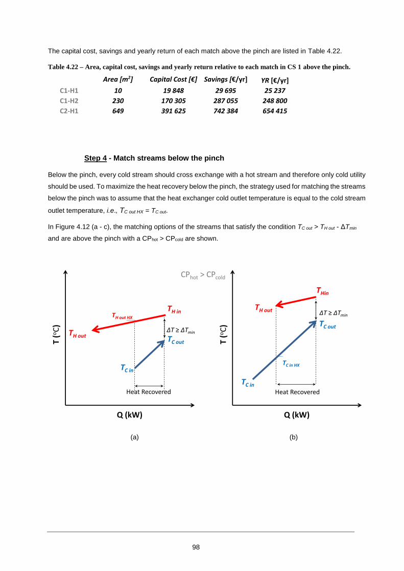
98

The capital cost, savings and yearly return of each match above the pinch are listed in Table 4.22.

Table 4.22 – Area, capital cost, savings and yearly return relative to each match in CS 1 above the pinch.

Area [m2] Capital Cost [€] Savings [€/yr] YR [€/yr]

C1-H1 10 19 848 29 695 25 237

C1-H2 230 170 305 287 055 248 800

C2-H1 649 391 625 742 384 654 415

Step 4 - Match streams below the pinch

Below the pinch, every cold stream should cross exchange with a hot stream and therefore only cold utility

should be used. To maximize the heat recovery below the pinch, the strategy used for matching the streams

below the pinch was to assume that the heat exchanger cold outlet temperature is equal to the cold stream

outlet temperature, i.e., TC out HX = TC out.

In Figure 4.12 (a - c), the matching options of the streams that satisfy the condition TC out > TH out - ΔTmin

and are above the pinch with a CPhot > CPcold are shown.

(a) (b)

Q (kW)

TH in

TH out TC out

TC in

T (o

C)

Heat Recovered

Q (kW)

T (o

C)

CPhot > CPcold

TH out HX

ΔT ≥ ΔTmin

THin

TH out

TC out

TC in

Heat Recovered

ΔT ≥ ΔTmin

TC in HX

99

(c)

Figure 4.12 – Possible cross-exchange scenarios when CPhot > CPcold with a pinch point for streams that are

below the pinch point.

Similarly, for CPhot < CPcold of pinched streams below the pinch, the possible scenarios are shown in

Figure 4.13 (a - d).

(a) (b)

Q (kW)

T (o

C)

CPhot > CPcold

THin

TH out

TC out

TC in

No Heat Transfer

ΔT < ΔTmin

Q (kW)

TH in

TH out

TC out

TC in

T (o

C)

Heat Recovered

ΔTmin

Q (kW)

THin

TH out

TC out

TC in

T (o

C)

Heat Recovered

ΔT ≥ ΔTmin

TC in HX

CPhot < CPcold

TH out HX TH out HX

100

(c) (d)

Figure 4.13 – Possible cross-exchange scenarios when CPhot < CPcold with a pinch point for streams that are

below the pinch point.

If streams are not pinched amongst them (TC out < TH out - ΔTmin) and are below the pinch then the possible

scenarios are shown in Figure 4.14(a - b).

(a) (b)

Figure 4.14 – Possible cross-exchange scenarios when streams are not pinched and are above the pinch point.

Q (kW)

TH in

TH out

TC out

TC in

T (o

C)

Heat Recovered

Q (kW)

THin

TH out

TC outTC inT

(oC

)

TC in HX

CPhot < CPcold

ΔT ≥ ΔTmin

ΔT < ΔTmin

No Heat Transfer

Q (kW)

TH in

TH out

TC out

TC in

T (o

C)

Heat Recovered

ΔT ≥ ΔTmin

Q (kW)

THin

TH out

TC out

TC in

T (o

C)

Heat Recovered

ΔT ≥ ΔTmin

TC in HX

TH in HX

Qhot < Qcold Qhot > Qcold

101

Taking into consideration the possible scenarios shown in Figure 4.12, Figure 4.4, Figure 4.13 and Figure

4.14, the algorithm for determining Q HX. Tc in HX, Tc out HX, Th in HX and Th out HX is detailed in Figure 4.15.


streams located below the pinch. The expression marked with an “*” is detailed in Appendix A2.

Input

Th out ; Th in ; Qh

Tc out ; Tc in ; Qc

ΔTmin

Calculate

CPc = Q c / (Tc out - Tc in)

CPh = Q h / (Th in - Th out)

Th in HX = Th in

Tc out HX = Tc out

N (Streams are not pinched)

CPc > CPh

?

Calculate

Q HX = Q HX = MIN [Q c, Q h]

Y

Tc out > Th out - ΔTmin

?

N Y

Th in - ΔTmin > Tc out

?

Y

Output

Match not

feasible

N

Output

Tc in HX ; Tc out HX

Th in HX ; Th out HX

Q HX

N

Calculate

Q HX = MIN [Q c, Q h]

Y

Calculate

Q HX = - CPc. CPh

. (Th in - Tc out - ΔTmin) / (CPh - CPc)

Calculate

Th out HX = - (Q HX / CPh ) + Th in HX

Tc in HX = - (Q HX / CPc ) + Tc out HX

- MIN [Q c, Q h] / CPc + Tc out + ΔTmin < - MIN [Q c, Q h] / CPh + Th in

?

*

102

As detailed before for the above pinch scenario, the described algorithm returns Q HX. Tc in HX, Tc out HX,

Th in HX, Th out HX. This information is used to determine the LMTD, A, Costyr and YR matrixes.

After the Yearly Return matrix is determined, select the cold stream with the highest outlet temperature,

i.e., closest to the pinch. For this stream, choose the match with the highest return and match the streams.

If there is no match with a positive return proceed to the next cold stream. Gradually move out of the pinch

until the cold stream with the lowest outlet temperature is matched.


For matching the streams bellow the pinch start with the cold streams with the highest outlet temperature.

In the case of CS 1, there is only one cold stream bellow the pinch so the matching sequence is

straightforward and all the matches have positive returns. Figure 4.16 shows the CS 1 network with all the

matches bellow the pinch.

Figure 4.16 – CS 1 network configuration, bellow the pinch, with all the streams duty fulfilled. Cold utility

consumption is 120 kW.

The capital cost, savings and yearly return of each match below the pinch are listed in Table 4.23Table

4.22.

Table 4.23 – Area, capital cost, savings and yearly return relative to each match in CS 1 below the pinch.


C1-H1 305 213 102 316 751 268 882

C1-H2 100 89 267 277 157 257 105

110 C

122 C

H2

122 C 60 CCP = 20 kW.C-1

110 C 30 C

C1

CP = 30 kW.C-1

H1

122 C 90 CCP = 40 kW.C-1 1280 kW

90 C

67 C

1120 kW

66 C

30 C

120 kW

103

Step 5 - Optimize temperature approach of heat exchangers at the pinch

After the streams are matched, the next step is to optimize the temperature approach of the streams that

are crossing the pinch to minimize the total annual cost, which is the sum of the annual capital cost and

the annual operating cost, as shown in Eq. (4.7). The annual capital cost corresponds to the annualized

investment and the operating cost corresponds to the annual cost spent on utilities.

𝑇𝑜𝑡 𝑎𝑛𝑛𝑢𝑎𝑙 𝑐𝑜𝑠𝑡[€] = 𝐴𝑛𝑛𝑢𝑎𝑙 𝑐𝑜𝑠𝑡𝑐𝑎𝑝[€] + 𝐴𝑛𝑛𝑢𝑎𝑙 𝑐𝑜𝑠𝑡𝑜𝑝[€]

(4.7)


The minimization is performed with Microsoft Excel Solver by manipulating the independent variables,

which are the stream temperatures at the pinch and the split stream ratios. In CS 1 there are no split

streams but in CS 2 it is possible to see an example where split streams are present.

Thus, the number of independent variables is equal to the number of streams that are crossing the pinch

plus the number of split stream minus 1.

In Figure 4.17, the network showing the independent variables to be optimized is shown. In the case of

CS1 there are 3 streams crossing the pinch and 0 splits, therefore there are 3 independent variables.

Figure 4.17 – CS 1 heat exchanger network, without heat being transferred across the pinch.

Table 4.24 presents a summary of the temperatures, duty, area, annual capital cost and operating cost

associated with each heat exchangers placed above and below the pinch without the optimization of the

independent variables.

H2180 C

170 C

165 C

C2

C1

H1

200 C 90 C40 kW.C-13000 kW

170 C

197 C

1160 kW

180 C

149 C

120 kW

200 C

153 C165 C

370 kW

1280 kW

90 C

67 C

1120 kW

66 C

30 C

120 kW

60 C

122 C

122 C

110 C

CP T

20 kW.C-1

30 kW.C-1

50 kW.C-1

60 C

110 C

30 C

T

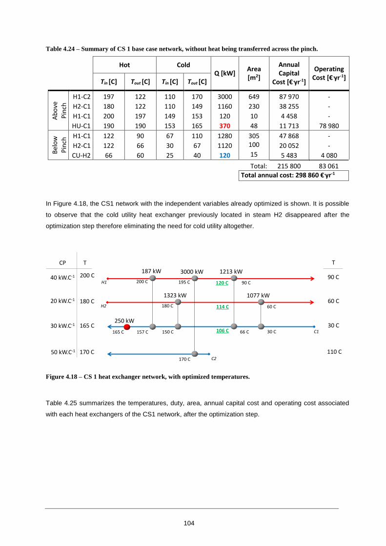
104

Table 4.24 – Summary of CS 1 base case network, without heat being transferred across the pinch.

Hot Cold Q [kW]

Area [m2]

Annual Capital

Cost [€.yr-1]

Operating Cost [€.yr-1]

Tin [C] Tout [C] Tin [C] Tout [C]

Ab

ove

P

inch

H1-C2 197 122 110 170 3000 649 87 970 -

H2-C1 180 122 110 149 1160 230 38 255 -

H1-C1 200 197 149 153 120 10 4 458 -

HU-C1 190 190 153 165 370 48 11 713 78 980

Bel

ow

P

inch

H1-C1 122 90 67 110 1280 305 47 868 -

H2-C1 122 66 30 67 1120 100 20 052 -

CU-H2 66 60 25 40 120 15 5 483 4 080

Total: 215 800 83 061

Total annual cost: 298 860 €.yr-1

In Figure 4.18, the CS1 network with the independent variables already optimized is shown. It is possible

to observe that the cold utility heat exchanger previously located in steam H2 disappeared after the

optimization step therefore eliminating the need for cold utility altogether.

Figure 4.18 – CS 1 heat exchanger network, with optimized temperatures.

Table 4.25 summarizes the temperatures, duty, area, annual capital cost and operating cost associated

with each heat exchangers of the CS1 network, after the optimization step.

H2180 C

170 C

165 CC1

H1

200 C 90 C40 kW.C-13000 kW

170 C

195 C

1323 kW

180 C

150 C

187 kW

200 C

157 C165 C

250 kW

1213 kW

90 C

66 C

1077 kW

60 C

30 C

120 C

114 C

106 C

CP T

20 kW.C-1

30 kW.C-1

50 kW.C-1

60 C

110 C

30 C

T

C2

105

Table 4.25 – Summary of CS 1 base case network, relaxing the pinch temperatures and allowing heat to be

transferred across the pinch.

Hot Cold Q [kW]

Area [m2]

Annual Capital

Cost [€.yr-1]


Tin [C] Tout [C] Tin [C] Tout [C]

Ab

ove

P

inch

H1-C2 195 120 110 170 3000 718 95 548 -

H2-C1 180 114 106 150 1323 329 50 780 -

H1-C1 200 195 150 153 187 17 5 941 -

HU-C1 190 190 153 165 250 35 9 314 53 365

Bel

ow

P

inch

H1-C1 120 90 66 106 1213 261 42 219 -

H2-C1 114 60 30 66 1077 113 21 893 -

Total: 225 694 53 365

Total annual cost: 279 059 €.yr-1

The methodology allowed the design of a heat exchanger network, which provided lower operating costs

that the more traditional pinch methodology used by the Pereira et al. [94] , as shown in Table 4.26.

Before the optimization step, the total operating cost provided by the methodology was 0.4% higher than

the result presented by the authors, while the result after the optimization step allowed the removal of the

cold utility and resulted in a 6.2% reduction in the annual cost when comparing with the annual cost

presented by the authors.

Table 4.26 – Comparison between the results achieved by the authors [94] and the proposed methodology for

CS 1.

ΔTmin [C]

Number of heat

exchangers

Annual Capital Cost

[€.yr-1]


Total annual cost [€.yr-1]

Annual cost

reduction

Authors [94] 8 6 214 510 83 084 297 595 0

With retrofit (not optimized) 12 7 215 800 83 061 298 860 +0.4%

With retrofit (optimized) 8 6 225 694 53 365 279 059 -6.2%

4.3 Case study 2 - Retrofit heat exchanger network (Industrial application)

The industrial case study is a system with 25 cold streams and 37 hot streams. Table 4.27 and Table

4.28 present the data regarding cold and hot streams, namely: the inlet (Tin) and outlet (Tout)

temperatures, heat capacity flow rate (CP), heat transfer coefficient (HTC) and heat load (Q).

106

Table 4.27 – Cold Stream data for CS 2.

Tin [C] Tout [C] CP [kW.C-1] Q [kW] HTC [kW.m-2.C-1]

C0 42.5 85.0 22.0 934.4 1.50

C1 30.7 58.9 46.8 1320.3 1.46

C2 -34.4 25.0 3.1 186.6 0.02

C3 187.2 188.1 6623.3 5961.0 0.20

C4 197.8 198.3 15572.8 7786.4 0.20

C5 196.0 202.0 50.3 301.9 0.20

C6 199.2 203.7 814.8 3666.7 1.39

C7 35.9 158.0 3.7 455.6 0.20

C8 163.0 187.0 9.4 226.1 0.20

C9 196.0 200.5 72.2 325.0 0.20

C10 149.6 150.2 3777.8 2266.7 0.20

C11 144.8 145.3 180.0 90.0 0.20

C12 32.0 88.0 0.8 46.9 0.20

C13 205.0 211.7 31.1 208.3 0.93

C14 25.0 198.0 0.1 15.2 0.03

C15 35.5 45.7 31.3 317.1 3.25

C16 33.2 101.5 9.1 620.8 4.15

C17 35.2 74.5 0.1 5.4 2.17

C18 39.8 63.3 30.2 708.8 1.58

C19 178.0 201.0 191.7 4409.0 0.20

C20 82.6 120.0 14.9 556.8 0.20

C21 82.6 120.0 14.9 556.8 0.20

C22 -37.9 -35.0 9.2 26.6 0.20

C23 -37.9 -31.0 10.7 74.1 0.20

C24 -37.9 -37.7 6.8 1.4 0.20

107

Table 4.28 – Hot Stream data for CS 2.

Tin [C] Tout [C] CP [kW.C-1] Q [kW] HTC [kW.m-2.C-1]

H0 -11.7 -37.0 10.7 270.0 0.20

H1 193.9 39.1 19.0 2941.1 1.26

H2 39.9 26.4 13.9 186.6 1.18

H3 68.0 54.9 100.9 1320.4 0.33

H4 70.0 50.0 57.4 1148.2 0.53

H5 -11.7 -34.4 3.3 74.1 0.03

H6 39.5 32.0 8.8 66.0 0.20

H7 51.4 39.0 287.7 3562.0 2.21

H8 109.1 32.0 52.8 4067.9 0.64

H9 138.0 39.5 19.0 1872.0 0.68

H10 99.8 99.7 46280.0 4628.0 0.20

H11 31.0 -31.0 0.4 26.6 0.20

H12 135.0 60.0 5.9 444.4 0.20

H13 144.2 100.0 149.2 6594.4 0.20

H14 185.2 34.0 3.0 457.8 0.20

H15 175.8 48.6 1.6 200.8 0.20

H16 35.1 28.0 92.1 650.0 0.20

H17 200.0 52.0 9.7 1430.6 0.20

H18 67.0 -13.0 0.0 1.4 0.20

H19 146.0 33.0 0.4 46.9 0.20

H20 33.0 32.0 0.7 0.7 0.20

H21 95.5 28.9 2.6 171.7 4.09

H22 100.3 74.9 0.2 5.4 0.20

H23 87.3 34.9 0.1 7.1 4.31

H24 82.5 37.6 33.5 1500.7 3.39

H25 118.2 48.0 36.8 2585.7 4.90

H26 118.5 85.0 52.4 1755.9 2.59

H27 99.7 35.0 5.1 327.6 0.20

H28 81.0 35.0 22.5 1037.0 1.85

H29 75.9 35.0 1.3 54.9 0.20

H30 110.0 46.0 29.3 1876.8 0.20

H31 95.5 54.0 15.2 633.2 0.20

H32 39.9 38.0 194.5 359.7 0.20

H33 42.8 38.0 185.8 888.3 0.20

H34 42.1 38.0 188.8 777.7 0.20

H35 121.0 113.0 31.0 248.0 0.20

H36 -17.0 -37.9 41.4 865.0 0.20

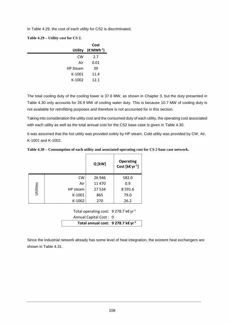
108

In Table 4.29, the cost of each utility for CS2 is discriminated.

Table 4.29 – Utility cost for CS 2.

Utility Cost

(€.MWh-1)

CW 2.7

Air 0.01

HP Steam 39

K-1001 11.4

K-1002 12.1

The total cooling duty of the cooling tower is 37.6 MW, as shown in Chapter 3, but the duty presented in

Table 4.30 only accounts for 26.9 MW of cooling water duty. This is because 10.7 MW of cooling duty is

not available for retrofitting purposes and therefore is not accounted for in this section.

Taking into consideration the utility cost and the consumed duty of each utility, the operating cost associated

with each utility as well as the total annual cost for the CS2 base case is given in Table 4.30.

It was assumed that the hot utility was provided solely by HP steam. Cold utility was provided by CW, Air,

K-1001 and K-1002.

Table 4.30 – Consumption of each utility and associated operating cost for CS 2 base case network.

Q [kW] Operating

Cost [k€.yr-1]

Uti

litie

s

CW 26 946 582.0

Air 11 470 0.9

HP steam 27 534 8 591.6

K-1001 865 79.0

K-1002 270 26.2

Total operating cost: 9 278.7 k€.yr-1

Annual Capital Cost : 0

Total annual cost: 9 278.7 k€.yr-1

Since the industrial network already has some level of heat integration, the existent heat exchangers are

shown in Table 4.31.

109

Table 4.31 – Existent heat exchanger data for cross exchange streams in the Estarreja MDI plant.

Cold

Stream Tin (C) Tout (C)

Hot Stream

Tin (C) Tout (C) Q (kW

C17-H22 PROCESS 35 74

PROCESS 100 75

5


PROCESS 100 37

317


PROCESS 118 101

621


PROCESS 146 33

47

C1-H3 PROCESS 31 59

PROCESS 68 55

1320

C2-H2 PROCESS -34 25

PROCESS 40 26

187

C0-H1 PROCESS 43 85

PROCESS 194 145

934

C22-H11 PROCESS -38 -31

PROCESS -12 -34

74

C23-H5 PROCESS -38 -35

PROCESS 31 -31

27

C24-H18 PROCESS -38 -38

PROCESS 67 -13

136

Taking into consideration the list given in Table 4.31 and the hot and cold stream data given in Table 4.27

and Table 4.28 and using the traditional pinch tools to identify the heat exchangers that crossing the

pinch, heat exchanger C0-H1 was identified as cross-pinching 710.2 KW. Therefore, this heat exchanger

was discarded and the streams that were used in this HX were used for crossing with other stream within

the network.

The values shown in Table 4.32 refer to the economic parameters. Parameters i and n are used in by

Eq. (4.5) to determine annualized factor whereas parameters a, b and c shall be used in Eq. (2.1) to

determine the capital cost of each heat exchanger.

Table 4.32 – Economic data regarding CS 2.

Rate of return (i) 13%

Plant Life (n) 10 yrs

Hours of operation per year 8000

a 40972

b 1947

c 0.7

110

Possible matches

As stated before, one the advantages of the proposed methodology is that it allows the user to define the

process incompatibilities and therefore eliminate the possibility of matching the defined streams. In Table

4.33, the feasibly matrix concerning CS2 network is given.

Table 4.33 – Feasibility matrix for the CS 2 network.

C0 C1 C2 C3 C4 C5 C6 C7 C8 C9 C10 C11 C12 C13 C14 C15 C16 C17 C18 C19 C20 C21 C22 C23 C24

H0

H1

H2

H3

H4

H5

H6

H7

H8

H9

H10

H11

H12

H13

H14

H15

H16

H17

H18

H19

H20

H21

H22

H23

H24

H25

H26

H27

H28

H29

H30

H31

H32

H33

H34

H35

H36

111

CS2 Step 1 - Determine process pinch temperature

To determine the process pinch, a 10 C global minimum approach (ΔTmin) was assumed, which is a

typical temperature approach for the chemical industry. The approach of each match will be individually

adjusted in a later step of the methodology, so this parameter is only important at this stage for

determining the position of each stream in regard to the pinch point.

The cold pinch temperature is 149.6 C and the hot pinch temperature is 159.6 C. In Table 4.34, the

temperatures and heat load of the streams above and below the pinch are presented. In the cases where

streams don’t show any value means that they are not crossing the pinch and therefore were not divided.

Cold streams C7 and C14 are crossing the pinch while the others are either above or below the pinch.

Stream C10 inlet temperature is exactly at the pinch.

Table 4.34 – Heat load and temperatures of cold streams of CS 2 above and below the pinch. A “-“ indicates

that there is no duty above or below the pinch. Streams with “*” are already cross-exchanging, so only the

duty that is being supplied by HU is considered.


Tin [C] Tout [C] Q [kW] Tin [C] Tout [C] Q [kW]

C0 - - - 42.5 85.0 934.4

*C1 - - - 58.9 58.9 0

*C2 - - - 25.0 25.0 0

C3 187.2 188.1 5961.0 - - -

C4 197.8 198.3 7786.4 - - -

C5 196.0 202.0 301.9 - - -

C6 199.2 203.7 3666.7 - - -

C7 149.6 158.0 31.3 35.9 149.6 424.2

C8 163.0 187.0 226.1 - - -

C9 196.0 200.5 325.0 - - -

C10 149.6 150.2 2266.7 - - -

C11 - - - 144.8 145.3 90.0

*C12 - - - 88.0 88.0 0

C13 205.0 211.7 208.3 - - -

C14 149.6 198.0 4.3 25.0 149.6 11.0

C15 - - - 35.5 45.7 0.1

*C16 - - - 101.5 101.5 0

*C17 - - - 74.5 74.5 0

C18 - - - 39.8 63.3 708.8

C19 178.0 201.0 4409.0 - - -

C20 - - - 82.6 120.0 556.8

C21 - - - 82.6 120.0 556.8

*C22 - - - -35.0 -35.0 0

*C23 - - - -31.0 -31.0 0

*C24 - - - -37.7 -37.7 0

112

Hot streams H1, H14, H15 and H17 are crossing the pinch while the others are below the pinch.

Table 4.35 – Heat load and temperatures of hot streams of CS 2 above and below the pinch. A “-“ indicates

that there is no duty above or below the pinch. Streams with “*” are already cross-exchanging, so only the

duty that is being removed by cold utility is considered.


Tin [C] Tout

[C] Q [kW]

Tin [C] Tout [C] Q [kW]

H0 - - - -11.7 -37.0 270.0

H1 193.9 159.6 651.2 159.6 39.1 2290.0

*H2 - - - 26.4 26.4 0

*H3 - - - 54.9 54.9 0

H4 - - - 70.0 50.0 1148.2

*H5 - - - -34.4 -34.4 0

H6 - - - 39.5 32.0 66.0

H7 - - - 51.4 39.0 3562.0

H8 - - - 109.1 32.0 4067.9

H9 - - - 138.0 39.5 1872.0

H10 - - - 99.8 99.7 4628.0

*H11 - - - -31.0 -31.0 0

H12 - - - 135.0 60.0 444.4

H13 - - - 144.2 100.0 6594.4

H14 185.2 159.6 77.5 159.6 34.0 380.3

H15 175.8 159.6 25.6 159.6 48.6 175.3

H16 - - - 35.1 28.0 650.0

H17 200.0 159.6 390.5 159.6 52.0 1040.1

*H18 - - - -13.0 -13.0 0

*H19 - - - 33.0 33.0 0

H20 - - - 33.0 32.0 0.7

H21 - - - 95.5 28.9 171.7

*H22 - - - 74.9 74.9 0

H23 - - - 87.3 34.9 7.1

H24 - - - 82.5 37.6 1500.7

*H25 - - - 101.3 48.0 1963.1

H26 - - - 118.5 85.0 1755.9

*H27 - - - 43.7 35.0 44.1

H28 - - - 81.0 35.0 1037.0

H29 - - - 75.9 35.0 54.9

H30 - - - 110.0 46.0 1876.8

H31 - - - 95.5 54.0 633.2

H32 - - - 39.9 38.0 359.7

H33 - - - 42.8 38.0 888.3

H34 - - - 42.1 38.0 777.7

H35 - - - 121.0 113.0 248.0

H36 - - - -17.0 -37.9 865.0

113

CS2 Step 2 - Split streams at the pinch according to pinch rules

Immediately above the pinch, the number of hot steams is lower than the number of cold streams.

Additionally, the CP of stream C2 is higher than the CP of stream H1. These conditions mean that there is

no necessity for splitting stream above the pinch.

Bellow the pinch, the number of hot steams is also lower than the number of cold streams, meaning that

one of the rules is not fulfilled and a hot stream should be split. If stream H3 is split in half, then the

number of hot stream will equal the number of cold streams and the CP of stream H3/1 and H3/2 is

higher than the CP of both stream C2 and C4. Table 4.36 and 4.37 show the results of applying the pinch

stream splitting rules to the CS 2 network.

Table 4.36 – Stream splitting rules for CS 2 regarding the number of streams immediately above/bellow the

pinch.


Nhot ≤ Ncold Nhot ≥ Ncold

Nhot = 4 > 3 = Ncold Nhot = 4 > 2 = Ncold

Table 4.37 – Stream splitting rules for CS 2 regarding the CP of streams immediately above/bellow the pinch.


CP hot ≤ CP cold CP hot ≥ CP cold

CPH1 < CPC10 CPH1,H17 > CPC7

CPH14 < CPC7,C10 CPH1,H14,H15,H17 > CPC14

CPH15 < CPC7,C10

CPH17 < CPC10

From Table 4.37, it is possible to observe that in the region above the pinch only tot cold streams, C7 and

C10, have a CP higher than the CP of the 4 hot streams. This means that two additional cold streams

with a CP higher than the CP of the hot streams are required. This is achieved by splitting stream C10 in

three, as shown in Figure 4.19. With the splits in place the Nhot ≤ Ncold condition is also fulfilled.

114

Figure 4.19 – CS2 streams crossing the pinch. Cold stream C10 with two splits.

CS2 Step 3 - Match streams above the pinch

After the Yearly Return matrix is determined, select the hot stream with the lowest outlet temperature, i.e.,

closest to the pinch. For this stream, choose the match with the highest return and match the streams. If

there is no match with a positive return proceed to the next hot stream. Gradually move out of the pinch

until the hot stream with the highest inlet temperature is matched.

In this step the streams above the pinch are matched according to the methodology. In Figure 4.20, the

matches above the pinch are shown.

H1

193.9 C 39.1 C

H14

185.2 C 34.0 C

149.6 C

159.6 C

H15

175.8 C 48.6 C

H17

200.0 C 52.0 C

149.6 CC10

150.2 C

198.0 C 25.0 C

C14

158.0 C 35.9 C

C7

CP = 3.7 kW.C-1

CP = 3777.8 kW.C-1

CP = 0.1 kW.C-1

CP = 19.0 kW.C-1

CP = 3.0 kW.C-1

CP = 1.6 kW.C-1

CP = 9.7 kW.C-1

CP = 1511 kW.C-1

CP = 756 kW.C-1

CP = 1511 kW.C-1

0.40.2

0.4

115

Figure 4.20 – CS 2 matches above the pinch.

Stream H1, H14 and H17 were matched with cold streams and all the duty above the pinch was fulfilled.

Stream H15 and C14 were not matched since there were not available matches that gave a positive

yearly return. This was mainly because the available duty above the pinch was only 25.6 kW for stream

H15 and 4.3 kW for stream C14, as seen in Table 4.35.

Three new heat exchangers were added to network above the pinch. It is assumed that hot utility heat

exchanger does not need to be replaced. In a further stage of analysis, it would be necessary to verify if

the overdimensioning of the heat exchanger would be problematic and, if yes, the cost of replacement must

also be accounted for in the economic analysis.

In Table 4.38, the capital cost, yearly savings and yearly return of the three matches above the pinch are

presented.

Table 4.38 – Yearly return relative to each match in CS 2 (above pinch)

H1

193.9 C

H14

185.2 C

149.6 C

159.6 C

H17

200.0 C

149.6 C

150.2 C

651.2 kW

77.5 kW

390.5 kW

193.9 C

159.6 C

159.6 C

159.6 C

C10/1

C10/2

C10/3

149.6 C

149.6 C

150.0 C

149.7 C

149.9 C

185.2 C

200 C

149.9 C

CP = 20 kW.C-1

CP = 40 kW.C-1

CP = 756 kW.C-1

CP = 1511 kW.C-1

CP = 1511 kW.C-1

CP = 9.7 kW.C-1

150.2 C

1157.5 kW


C10/1-H1 158 104 500 203 217 183 959

C10/2-H14 39 64 520 24 188 12 298

C10/3-H17 165 102 400 121 868 102 997

116

CS2 Step 4 - Match streams below the pinch

After the Yearly Return matrix is determined, select the cold stream with the highest outlet temperature,

i.e., closest to the pinch. For this stream, choose the match with the highest return and match the streams.

If there is no match with a positive return proceed to the next cold stream. Gradually move out of the pinch

until the cold stream with the lowest outlet temperature is matched.

Figure 4.21 – CS 2 matches bellow the pinch.

Four new heat exchangers were added to the network below the pinch. Again, like in the above pinch case,

it is considered that, although overdimensioned, the existent cooling utility heat exchangers can still be

used and don’t need to be replaced.

In Table 4.39, the capital cost, yearly savings and yearly return of the three matches below the pinch are

presented.

149.6 C

159.6 C

H1

H13

H26

159.6 CCP = 19 kW.C-1

144.2 C

118.5 C

CP = 149 kW.C-1

CP = 52 kW.C-1

424.2 kW

137.3 C

556.8 kW

149.6 CCP = 52 kW.C-1

35.9 C

120.0 CCP = 15 kW.C-1

82.6 C

140.5 C

556.8 kW

136.7 C

82.6 C

120.0 CCP = 15 kW.C-1

934.4 kW

88.1 C

42.0 C

85.0 CCP = 22 kW.C-1

708.8 kW

105.0 C

39.8 C

63.2 CCP = 30 kW.C-1

39.1 C

100.0 C

85.0 C

35.9 C

82.6 C

82.6 C

42.0 C

39.8 C

C0

C7

C20

C21

C18

1047.1 kW

85.0 C

5480.9 kW

100.0 C

931.3 kW

39.1 C

117

Table 4.39 – Yearly return relative to each match in CS 2 (below pinch)

CS2 Step 5 - Optimize temperature approach of heat exchangers at the pinch

In this step, the independent variables are optimized so that the total annual cost of the network is minimal.

Since the number of independent variables is equal to the number of streams that are crossing the pinch

plus the number of split stream minus 1, in the case of CS2 the number of streams crossing the pinch is 4

(H1, H14, H17 and C7) and the number of splits is 3, which result in the total of 4 + 3 - 1 = 6 independent

variables.

In Figure 4.22, the retrofitted network, without temperature approach optimization yet performed, is

shown. The independent variables are the variables in green.


A summary of each utility heat duty and associated operating costs for the retrofitted network, without

independent variables optimization, is shown in Table 4.40.

H1

H13

H26

193.9 CCP = 19 kW.C-1

144.2 C

118.5 C

CP = 149 kW.C-1

CP = 52 kW.C-1

424.2 kW

137.3 C

556.8 kW

158.0 CCP = 52 kW.C-1

120.0 CCP = 15 kW.C-1

82.6 C

140.5 C

556.8 kW

136.7 C

82.6 C

120.0 CCP = 15 kW.C-1

934.4 kW

88.1 C

42.0 C

85.0 CCP = 22 kW.C-1

708.8 kW

105.0 C

63.2 C

63.2 CCP = 30 kW.C-1

39.1 C

100.0 C

85.0 C

35.9 C

82.6 C

82.6 C

42.0 C

39.8 C

C0

C7

C20

C21

C18

1047.1 kW

85.0 C

5480.9 kW

100.0 C

931.3 kW

39.1 C

0.40.2

0.4

H14

185.2 C

H17

200.0 C

77.5 kW

390.5 kW

CP = 3 kW.C-1

CP = 10 kW.C-1

150.2 CCP = 3778 kW.C-1

651.2 kW

159.6 C

150.0 C

149.7 C

149.9 C

149.9 C150.2 C

380.3 kW

34.0 C

1040.1 kW

52.0 C

C10

34.0 C

52.0 C

159.6 C

159.6 C

1147.5 kW

149.6 C

31.3 kW

158.0 C

149.6 C

118.5 C

85.0 C

39.8 C

120.0 C

120.0 C

193.9 C

144.2 C

185.2 C

200.0 C

149.6 C

35.9 C


C7-H1 62 73 666 132 393 118 817

C20-H13 144 98 969 173 755 155 516

C21-H13 161 103 469 173 755 154 686

C0-H1 28 59 854 291 606 280 576

C18-H26 12 51 601 221 191 211 682

118

Table 4.40 – Summary of CS 2 base case network. Retrofit without optimization.

Retrofit without optimization

Q [kW] Operating

Cost [k€.yr-1]

CW 8 880 191.8

HP steam 1 179 367.8

Total operating cost 559.6 k€.yr-1

Total capital cost 659.4 k€

Annual capital cost 121.5 k€.yr-1

Total annual cost 681.1 k€.yr-1

Next, the independent variables are changed so that the total annual cost is minimized. This minimization

was performed using Microsoft Excel Solver [90], changing the independent variables and setting the

objective as minimization of the total annual cost (a more comprehensive explanation of the tool is detailed

in Appendix A3).

Figure 4.23 – CS 2 heat exchanger network, with optimized temperatures.

The optimization step does not take into account the previously imposed ΔTmin and the independent

variables are manipulated so that the total annual cost of the network is minimized. The resulting network

has a ΔTmin of 0.8 C in heat exchanger C10/1-H1. Although this temperature approach is not very typical

the fact that the heat transfer coefficient of stream H1, 1.26 kW.m-2.C-1, is relatively high results in this

network configuration.

H1

H13

H26

193.9 CCP = 19 kW.C-1

144.2 C

118.5 C

CP = 149 kW.C-1

CP = 52 kW.C-1

422.7 kW

128.1 C

556.8 kW

158.0 CCP = 52 kW.C-1

120.0 CCP = 15 kW.C-1

82.6 C

140.5 C

556.8 kW

136.7 C

82.6 C

120.0 CCP = 15 kW.C-1

934.4 kW

79.0 C

42.0 C

85.0 CCP = 22 kW.C-1

708.8 kW

105.0 C

63.2 C

63.2 CCP = 30 kW.C-1

39.1 C

100.0 C

85.0 C

35.9 C

82.6 C

82.6 C

42.0 C

39.8 C

C0

C7

C20

C21

C18

1047.1 kW

85.0 C

5480.9 kW

100.0 C

757.6 kW

39.1 C

0.530.12

0.35

H14

185.2 C

H17

200.0 C

102.4 kW

476.2 kW

CP = 3 kW.C-1

CP = 10 kW.C-1

150.2 CCP = 3778 kW.C-1

826.4 kW

150.4 C

150.0 C

149.8 C

150.0 C

149.9 C150.2 C

355.3 kW

34.0 C

954.4 kW

52.0 C

C10

34.0 C

52.0 C

151.4 C

150.7 C

861.6 kW

149.2 C

32.8 kW

158.0 C

149.6 C

118.5 C

85.0 C

39.8 C

120.0 C

120.0 C

193.9 C

144.2 C

185.2 C

200.0 C

149.6 C

35.9 C

119

The capital cost, savings and yearly return of each match after temperature optimization are listed in

Table 4.41.

Table 4.41 – Area, capital cost, savings and yearly return relative to each match in CS 2. After temperature

optimization


C10/1-H1 370 151 295 148 601 120 719

C10/2-H14 92 83 606 31 958 16 551

C10/3-H17 449 167 025 257 902 227 121

C7-H1 177 91 329 131 929 115 098

C20-H13 144 98 969 173 755 155 516

C21-H13 160 103 469 173 755 154 686

C0-H1 34 62 728 291 606 280 046

C18-H26 12 51 601 221 191 211 682

A summary of each utility heat duty and associated operating costs for the retrofitted network, after

optimization, is shown in Table 4.42.

Table 4.42 – Summary of CS 2 base case network. Retrofit with optimization

Retrofit with optimization

Q [kW] Operating

Cost [k€.yr-1]

CW 8 595 185.7

HP steam 894 279.1

Total operating cost 464.8 k€.yr-1

Total capital cost 810.0 k€

Annual capital cost 149.3 k€.yr-1

Total annual cost 614.0 k€.yr-1

For the abovementioned scenario stream C10 was split and the outlet temperature of each split stream was

not fixed. This situation is normal when there is no phase change. However, when working with reboilers

or condensers, the outlet temperature should be the same for all split streams since there is a phase change.

In these cases, the hot/cold utility is in parallel with the other split streams.

If this consideration is taken into account in the case of stream C10 and the outlet temperature of each split

stream is fixed than the split fractions are no longer be an independent variables and the CS 2 network

would be as shown in Figure 4.24. In this case, the heat exchanger with the hot utility in stream C10 is

placed in parallel with the other heat exchangers.

120

The number of independent variables also changes from 6 to 4 as the split ratio is calculated instead of

being an independent variable. This is because the in- and outlet temperatures are fixed and, for fulfilling a

given heat duty, the split ratio is calculated and is no longer a variable that can be varied.


Stream C10 split streams with fixed outlet temperatures.

The optimized network is shown in Figure 4.25.

Figure 4.25 – CS 2 heat exchanger network, with optimized temperatures. Stream C10 split streams with

fixed outlet temperatures.

H1

H13

H26

193.9 CCP = 19 kW.C-1

144.2 C

118.5 C

CP = 149 kW.C-1

CP = 52 kW.C-1

424.2 kW

137.3 C

556.8 kW

158.0 CCP = 52 kW.C-1

120.0 CCP = 15 kW.C-1

82.6 C

140.5 C

556.8 kW

136.7 C

82.6 C

120.0 CCP = 15 kW.C-1

934.4 kW

88.1 C

42.0 C

85.0 CCP = 22 kW.C-1

708.8 kW

105.0 C

63.2 C

63.2 CCP = 30 kW.C-1

39.1 C

100.0 C

85.0 C

35.9 C

82.6 C

82.6 C

42.0 C

39.8 C

C0

C7

C20

C21

C18

1047.1 kW

85.0 C

5480.9 kW

100.0 C

931.3 kW

39.1 C

0.17

H14

185.2 C

H17

200.0 C

77.5 kW

390.5 kW

CP = 3 kW.C-1

CP = 10 kW.C-1

150.2 CCP = 3778 kW.C-1

651.2 kW

159.6 C

380.3 kW

34.0 C

1040.1 kW

52.0 C

C10

34.0 C

52.0 C

159.6 C

159.6 C

1147.5 kW

149.6 C

31.3 kW

158.0 C

149.6 C

118.5 C

85.0 C

39.8 C

120.0 C

120.0 C

193.9 C

144.2 C

185.2 C

200.0 C

149.6 C

35.9 C

150.2 C

0.51

0.03

0.29

H1

H13

H26

193.9 CCP = 19 kW.C-1

144.2 C

118.5 C

CP = 149 kW.C-1

CP = 52 kW.C-1

158.0 CCP = 52 kW.C-1

120.0 CCP = 15 kW.C-1

120.0 CCP = 15 kW.C-1

85.0 CCP = 22 kW.C-1

63.2 CCP = 30 kW.C-1

39.1 C

100.0 C

85.0 C

35.9 C

82.6 C

82.6 C

42.0 C

39.8 C

C0

C7

C20

C21

C18

85.0 C

100.0 C

39.1 C

0.21

H14

185.2 C

H17

200.0 C

CP = 3 kW.C-1

CP = 10 kW.C-1

150.2 CCP = 3778 kW.C-1

34.0 C

52.0 C

C10

34.0 C

52.0 C

861.7 kW

32.8 kW

158.0 C

149.6 C149.6 C150.2 C

0.38

0.05

0.36

422.7 kW

128.1 C

556.8 kW

140.5 C

556.8 kW

136.7 C

934.4 kW

79.0 C

42.0 C

708.8 kW

105.0 C

1047.1 kW

5480.9 kW

757.6 kW

102.4 kW

476.2 kW

826.4 kW

150.4 C

355.3 kW

954.4 kW151.4 C

150.7 C

118.5 C

85.0 C

193.9 C

144.2 C

185.2 C

200.0 C

149.2 C 35.9 C

82.6 C

82.6 C

63.2 C 39.8 C

120.0 C

120.0 C

121

For this specific heat exchanger network, the total annual cost is similar independently of fixing the split

streams outlet temperatures or not. Nonetheless, it is important to present both approaches as it might be

relevant when applying the methodology to other networks.

Table 4.43 compares the utility duty, total operating cost, annual capital cost and total annual cost for the

different scenarios. The base case scenario, which has several exchangers that are violating pinch rules,

has the highest total annual cost of 1540.3 k€.yr-1. After retrofitting the network with the stream matching

methodology the total annual cost of the network was reduced to 681.1 k€.yr-1. After optimizing the network

a 614.0 k€.yr-1 total annual cost was achieved. The total operating cost is reduced by 1075 k€.yr-1 when

comparing the base case with the optimized network.

Table 4.43 – Summary of CS 2 base case network. Retrofit with optimization.

Base case

Retrofit without optimization

Retrofit with optimization

Q [kW] Operating

Cost [k€.yr-1]

Q [kW]

Operating Cost [k€.yr-1]

Q [kW] Operating

Cost [k€.yr-1]

CW 12 245 264.5 8 878 191.8 8 595 185.7

HP steam 4 089 1 275.8 1 148 358.0 862 268.9

Total operating cost 1 540.3 k€.yr-1 559.6 k€.yr-1 464.8 k€.yr-1

- 659.4 k€ 810.0 k€

Annual capital cost - 121.5 k€.yr-1 149.3 k€.yr-1

Total annual cost 1 540.3 k€.yr-1 681.1 k€.yr-1 614.0 k€.yr-1

It is possible to apply the methodology for retrofitting industrial networks. The results summarized in Table

4.44 show that applying the methodology without the optimization step allows a 56.4% annual cost

reduction and, with the optimization step, allows a further 7.7% reduction when comparing with the base

case scenario.


Considers only the streams that were subject to retrofit.

Annual cost [k€.yr-1] Annual cost reduction

Base case 1 540.3 0

With retrofit 671.3 -55.8%

With retrofit (optimized) 603.8 -63.5%

Table 4.45 summarizes the annual cost of the base case, with retrofit and with retrofit (optimized) networks

but, differently from Table 4.44 that considers only the streams that were subject to retrofit efforts, considers

the whole network. The overall reduction on the annual cost after optimization is 11.3% when compared to

the base case scenario.

122


Considers the whole network.

Annual cost [k€.yr-1] Annual cost reduction

Base case 9 278.7 0

With retrofit 8 301.3 -10.5%

With retrofit (optimized) 8 234.2 -11.3%

4.4 Impact on cooling tower operation

Adding to the fact that the total annual cost will be reduced, the cooling tower will also operate under the

design limit during a higher percentage of the year. In Chapter 3, a plot showing the variation of the cooling

water supply temperature with the air wet-bulb temperature was presented. If the retrofit measures were to

be implemented the cooling water range would decrease from 6 C to 5.5 C, meaning that the network would

still operate within the design limit of 26 C for the cooling water supply temperature with an air wet-bulb

temperature of 21.5 C (Figure 4.26).

Figure 4.26 – Cooling water supply temperature vs Air wet bulb temperature for the Dow’s cooling tower

with the retrofit measures implemented.

23.5

24

24.5

25

25.5

26

26.5

27

27.5

18 19 20 21 22 23

Co

olin

g W

ater

Su

pp

ly t

emp

erat

ure

(C

)

Air Wet-Bulb Temperature (C)

Range = 6.5 C

Range = 6.0 C

Range = 5.5 C

123

Looking at Figure 4.27, it is possible to observe that if the retrofit measures were implemented the cooling

tower would only be above its design limit during 3% of the year instead of 4.5% for the base case scenario.

Figure 4.27 – Estimated wet-bulb temperature frequency of occurrence in 2010 at Dow’s Estarreja MDI plant

with the retrofit measures implemented.

4.5 Impact on the steam network

LP steam can be produced by either flashing HP condensates or by letting down HP steam. This has clear

impacts on the plant overall energy analysis as reducing LP steam is only advantageous to the point where

LP steam is only related to the steam that is being generated by the let-down valve. Considering the case

124

where a process optimization would lead to a situation where no letdown would be necessary, if LP steam

consumption was further reduced without carrying out any other modification in the system, LP steam

header pressure would increase and vent to atmosphere, consequently rendering this reduction useless.

When evaluating any process modification, it is necessary to analyze how it will impact on the steam

network balance. It is therefore necessary to assess the overall heat and mass balance of the steam

network and check if no LP steam will be vented to the atmosphere.

Updating the thermodynamic model presented in Chapter 3 with the optimized network scenario a new

process flowsheet was calculated as shown in Figure 4.28. Some important differences between the steam

network process flowsheet before (Figure 3.35) and after (Figure 4.28) the implementation of the stream

match methodology arise. It is possible to observe that HP to LP steam letdown dropped from 3324 kg/h to

12 kg/h, meaning that all the LP steam requirements are being met by flashing the HP condensates in the

LP flash drum. Total make-up water decreased from 5691 kg/h to 5466 kg/h and it was possible to eliminate

the vented steam from the atmospheric flash drum.

Figure 4.28 – Steam network block diagram after implementing optimized network scenario.

The resulting steam network is balanced in terms of HP and LP steam consumption. However, if further

actions were taken to reduce LP steam consumption an unbalanced situation would arise due to the

overproduction of LP steam by flashing the HP condensates. To avoid this situation, a possible solution

would be to install a new HP knock out drum that would separate the HP condensate phases and pump

the condensate directly to the boiler and the vapor phase to the LP steam header. Depending on the LP

steam consumption, the HP condensate would either go directly to the boiler, for lower LP steam

requirements, or to the LP flash drum, for higher LP steam requirements. The proposed scheme is

presented in Figure 4.29.

LP consumers

HP consumers

Deaerator

41323 kg/h

41311 kg/h

5886 kg/h

12 kg/h

950 kg/h

35425 kg/h

237 kg/h


Boiler500 kg/h

Blowdown

Make-up water

0 kg/hTo Atm

562 kg/h

4904 kg/h799 kg/h

155 kg/hTo Atm

100 kg/hCondensate

export

LPFlash Drum

AtmFlash Drum

let down

125

Figure 4.29 – Steam network configuration that allows the control of LP steam generated in the LP flash

drum.

LP consumers

HP consumers

Deaerator

46569 kg/h

43245 kg/h

6161 kg/h

1140 kg/h

37084 kg/h

3644 kg/h


Boiler500 kg/h

Blowdown

Make-up water

237 kg/hTo Atm

589 kg/h

5112 kg/h3976 kg/h

143 kg/hTo Atm

100 kg/hCondensate

export

LPFlash Drum

AtmFlash Drum

HPFlash Drum

let down3324kg/h

126

5 Conclusions and Recommendations

5.1 General conclusions

The approach suggest a methodology for the implementation of the cooling water and steam systems

models. These models allow the performance evaluation of existent networks and serve as a basis for

optimization studies. Furthermore, a heat integration methodology was developed that aimed for the

reduction of utilities consumption.

A new approach based on an equilibrium stage method for modeling an existent cooling towers was

developed and validated with experimental data, both from previous works and data collected from an

industrial facility [76]. The presented methodology can be implemented in ASPEN PLUS models and

integrated with the cooling water network model.

To develop an accurate model of the cooling system the flow on each point of the network was required

and for that a hydraulic model of the cooling water network was implemented. The hydraulic model not

only permitted the calculation of the accurate flow on each point of the network but also allowed the

identification and improvement of heat exchangers where the cooling water flow differed from design.

The models of the case study plant suggested that the maximum wet-bulb temperature after which the

cooling tower is not able to supply cooling water at a temperature lower then design was 20.5 C which, for

the year of 2010, corresponded to 4.5% of the time.

A framework for analyzing the steam generators’ performance was also presented. This methodology

allows the performance evaluation of the steam generators as well as the multiple steam generators system

optimization by managing the load of each steam generator. It was shown that using the direct method for

determining boiler performance rendered better results that using the direct method due to the high variation

in steam flow measurement.

For the boilers operation it was found that distributing the load across the three boilers was the better option

and stopping a boiler while increasing the load of the other two did not add significant savings. Additionally,

operating with only two boilers would also decrease reliability of the plant.

A detailed description of the steps taken for the implementation of the steam system thermodynamic model

in ASPEN PLUS was also presented in this chapter. This model is used to build the steam network process

flowsheet. The case study network has 3314 kg/h of LP steam that can be reduced before any change has

to be implemented on the steam network configuration to avoid venting LP steam to atmosphere.

A new methodology for heat integration based on pinch analysis concepts was described in Chapter 4. The

procedure can be used for the grassroots design or for retrofitting a heat exchanger network.

The stream match methodology takes into account forbidden matches and describes how the network is

built in a sequential manner considering the yearly return of each match. The last step of the methodology

is to “relax” the ΔTmin that was imposed at the beginning of the design phase and optimize the independent

127

variables, which are the pinch temperatures and split ratios, to minimize the overall yearly cost of the

network.

The methodology was applied to a grassroots design of a network with 2 hot and 2 cold streams and the

resulting network had an annualized cost 6.2% lower than the configuration achieved by Pereira et al. [94]

who used traditional design pinch methodology.

For retrofitting an industrial network the approach was to determine which heat exchangers were violating

any of the pinch rules and apply the stream matching methodology to the streams that were being serviced

by these heat exchangers. In terms of annual cost the retrofitted network was 11.3% more efficient than

the base case scenario. An investment of 810.0 k€ would represent savings of 1075 k€/yr, meaning a

payback of less than 1 year.

The models of the steam and cooling water systems were used to evaluate the performance of the

retrofitted industrial network. It was found that the cooling tower would be underdimensioned during 3% of

the year instead of the 4.5% of the base case scenario. As for the steam network the HP steam let-down

to generate LP steam would be reduced from 3324 kg/h to 12 kg/h and demineralized water consumption

from 5691 kg/h to 5466 kg/h.

5.2 Recommendations for future work

Some of the themes addressed in this work can be subject of further study and development. Energy

integration in industrial facilities is a relevant field of study that will most certainly remain actual in the

foreseeable future.

A model of the cooling tower using equilibrium stage was developed in ASPEN PLUS. Such model could

also be formulated using thermodynamic equilibrium equations and then be used in other platforms other

than ASPEN PLUS. The cooling tower model could then be integrated into mathematical formulations

regarding cooling water systems.

The methodology for evaluating the performance of the steam generators using the indirect method and for

optimizing load distribution was presented. This methodology should be applied to other case studies where

the performance of each steam generator differ from one another.

As for the stream match methodology it would be interesting to apply the methodology to other case studies

to further validate it. Also, the developed tools can be automated to turn them into an integrated user-

friendly tool that uses the concepts of the stream matching methodology. This tool could be of great value

for designing and retrofitting industrial facilities.

128

6 References

[1] Key World Energy Statistics Report. International Energy Agency 2015

[2] Polyurethane MDI Handbook. BASF Corporation 2000.

[3] R. Sood, J.-L. Roser, R. De Genova. Advances in pure and polymeric MDI chemistry to meet changing

product, process and performance needs. Utech Asia '97, Singapore, 1997.

[4] F.J.M. Neves. Modelling and Optimization of Large-Scale Processes—Application to the liquid-phase

aniline production. Departamento de Engenharia Química. Faculdade de Ciências e Tecnologia da

Universidade de Coimbra 2007.

[5] S.R. Wan Alwi, N.E. Mohammad Rozali, Z. Abdul-Manan, J.J. Klemeš. A process integration targeting

method for hybrid power systems. Energy. 44 (2012) 6-10.

[6] S.-G. Yoon, J. Lee, S. Park. Heat integration analysis for an industrial ethylbenzene plant using pinch

analysis. Applied Thermal Engineering. 27 (2007) 886-93.

[7] M. Ebrahim, A. Kawari. Pinch technology: an efficient tool for chemical-plant energy and capital-cost

saving. Applied Energy. 65 (2000) 45-9.

[8] T. Gundersen. International Energy Agency. Implementating agreement on process integration. Annex

I - A Process Integration Primer. SINTEF Energy Research 2000.

[9] B. Linnhoff, D.R. Mason, I. Wardle. Understanding heat exchanger networks. Computers & Chemical

Engineering. 3 (1979) 295-302.

[10] B. Linnhoff, J.R. Flower. Synthesis of heat exchanger networks: I. Systematic generation of energy

optimal networks. AIChE Journal. 24 (1978) 633-42.

[11] B. Linnhoff, J.R. Flower. Synthesis of heat exchanger networks: II. Evolutionary generation of

networks with various criteria of optimality. AIChE Journal. 24 (1978) 642-54.

[12] J.J. Klemeš. Handbook of Process Integration (PI): Minimisation of Energy and Water Use, Waste

and Emissions - Process Integration (PI): An Introduction. Woodhead Publishing Limited 2013.

[13] Aspen Plus V7.3 [25.0.1.5015]. Aspen Technology Inc. 2011.

129

[14] F. Benyahia. Flowsheeting packages: reliable or fictitious process models? Trans IChemE. 78

(2000).

[15] F.G. Martins. "Process simulators". Engenharia de processos e sistemas; Programa doutoral em

Engenharia da Refinação, Petroquímica e Química 2010.

[16] A.C. Dimian. Integrated design and simulation of chemical processes 2003.

[17] Structural representations of systems. Norwegian University of Science and Technology. Notes of

TKP9 & KP8100 2007 course, 2007.

[18] S.H. Kim, S.G. Yoon, S.H. Chae, S. Park. Economic and environmental optimization of a multi-site

utility network for an industrial complex. Journal of environmental management. 91 (2010) 690-705.

[19] J.-K. Kim, R. Smith. Cooling water system design. Chemical Engineering Science. 56 (2001) 3641-

58.

[20] M.H. Agha, R. Thery, G. Hetreux, A. Hait, J.M. Le Lann. Integrated production and utility system

approach for optimizing industrial unit operations. Energy. 35 (2010) 611-27.

[21] W.S. Goh, Y.K. Wan, C.K. Tay, R.T.L. Ng, D.K.S. Ng. Automated targeting model for synthesis of

heat exchanger network with utility systems. Applied Energy. 162 (2016) 1272-81.

[22] G.-Y. Jin, W.-J. Cai, L. Lu, E.L. Lee, A. Chiang. A simplified modeling of mechanical cooling tower for

control and optimization of HVAC systems. Energy Conversion and Management. 48 (2007) 355-65.

[23] D.J. Benton, C.F. Bowman , M. Hydeman, P. Miller. An improved cooling tower algorithm for the

CoolTools simulation model. ASHRAE Transactions. 108 (2002) AC-02-9-4.

[24] J.C. Kloppers, D.G. Kröger. A critical investigation into the heat and mass transfer analysis of

counterflow wet-cooling towers. International Journal of Heat and Mass Transfer. 48 (2005) 765-77.

[25] J.R. Picardo, J.E. Variyar. The Merkel equation revisited: A novel method to compute the packed

height of a cooling tower. Energy Conversion and Management. 57 (2012) 167-72.

[26] M.M. Castro, T.W. Song, J.M. Pinto. Minimization of Operational Costs in Cooling Water Systems.

Chemical Engineering Research and Design. 78 (2000) 192-201.

[27] J.-U.-R. Khan, B.A. Qureshi, S.M. Zubair. A comprehensive design and performance evaluation

study of counter flow wet cooling towers. International Journal of Refrigeration. 27 (2004) 914-23.

130

[28] R. Al-Waked, M. Behnia. CFD simulation of wet cooling towers. Applied Thermal Engineering. 26

(2006) 382-95.

[29] E. Rubio-Castro, M. Serna-González, J.M. Ponce-Ortega, M.A. Morales-Cabrera. Optimization of

mechanical draft counter flow wet-cooling towers using a rigorous model. Applied Thermal Engineering.

31 (2011) 3615-28.

[30] M. Hosoz, H.M. Ertunc, H. Bulgurcu. Performance prediction of a cooling tower using artificial neural

network. Energy Conversion and Management. 48 (2007) 1349-59.

[31] T.-H. Pan, S.-S. Shieh, S.-S. Jang, W.-H. Tseng, C.-W. Wu, J.-J. Ou. Statistical multi-model

approach for performance assessment of cooling tower. Energy Conversion and Management. 52 (2011)

1377-85.

[32] M. Serna-González, J.M. Ponce-Ortega, A. Jiménez-Gutiérrez. MINLP optimization of mechanical

draft counter flow wet-cooling towers. Chemical Engineering Research and Design. 88 (2010) 614-25.

[33] R.V. Rao, V.K. Patel. Optimization of mechanical draft counter flow wet-cooling tower using artificial

bee colony algorithm. Energy Conversion and Management. 52 (2011) 2611-22.

[34] X. Qi, Y. Liu, Q. Guo, J. Yu, S. Yu. Performance prediction of seawater shower cooling towers.

Energy. 97 (2016) 435-43.

[35] M.H. Sadafi, S. González Ruiz, M.R. Vetrano, I. Jahn, J. van Beeck, J.M. Buchlin, et al. An

investigation on spray cooling using saline water with experimental verification. Energy Conversion and

Management. 108 (2016) 336-47.

[36] J.M. Ponce-Ortega, M. Serna-González, A. Jiménez-Gutiérrez. MINLP synthesis of optimal cooling

networks. Chemical Engineering Science. 62 (2007) 5728-35.

[37] K.V. Gololo, T. Majozi. On Synthesis and Optimization of Cooling Water Systems with Multiple

Cooling Towers. Industrial & Engineering Chemistry Research. 50 (2011) 3775-87.

[38] J. Sun, X. Feng, Y. Wang. Cooling-water system optimisation with a novel two-step sequential

method. Applied Thermal Engineering. 89 (2015) 1006-13.

[39] S.-C. Georgescu, A.-M. Georgescu, A. Jumara, V.-F. Piraianu, G. Dunca. Numerical Simulation of

the Cooling Water System of a 115 MW Hydro-Power Plant. Energy Procedia. 85 (2016) 228-34.

131

[40] M. Kljajić, D. Gvozdenac, S. Vukmirović. Use of Neural Networks for modeling and predicting boiler's

operating performance. Energy. (2012).

[41] S.K. Behera, E.R. Rene, M.C. Kim, H.-S. Park. Performance prediction of a RPF-fired boiler using

artificial neural networks. International Journal of Energy Research. 38 (2014) 995-1007.

[42] D. Strušnik, M. Golob, J. Avsec. Artificial neural networking model for the prediction of high efficiency

boiler steam generation and distribution. Simulation Modelling Practice and Theory. 57 (2015) 58-70.

[43] Ø. Andreassen, T.O. Olsen. Optimal Load Allocation. Modeling, Identification and Control: A

Norwegian Research Bulletin. 4 (1983) 107-16.

[44] A.C. Dunn, Y.Y. Du. Optimal load allocation of multiple fuel boilers. ISA transactions. 48 (2009) 190-

5.

[45] C.D. Rocco, R. Morabito. Um modelo de otimização para as operações de produção de vapor em

caldeiras industriais. Gestao e Producao. 19 (2012) 273-86.

[46] C.-L. Chen, H.-C. Chen. A mathematical approach for retrofit and optimization of total site steam

distribution networks. Process Safety and Environmental Protection. 92 (2014) 532-44.

[47] Y. Majanne. Model predictive pressure control of steam networks. Control Engineering Practice. 13

(2005) 1499-505.

[48] S.W.A. Coetzee, T. Majozi. Steam System Network Synthesis Using Process Integration. Industrial &

Engineering Chemistry Research. 47 (2008) 4405-13.

[49] W. Zhong, H. Feng, X. Wang, D. Wu, M. Xue, J. Wang. Online hydraulic calculation and operation

optimization of industrial steam heating networks considering heat dissipation in pipes. Energy. 87 (2015)

566-77.

[50] T. Umeda, T. Harada, K. Shiroko. A thermodynamic approach to the synthesis of heat integration

systems in chemical processes. Computers & Chemical Engineering. 3 (1979) 273-82.

[51] T.F. Yee, I.E. Grossmann. Simultaneous optimization models for heat integration—II. Heat

exchanger network synthesis. Computers & Chemical Engineering. 14 (1990) 1165-84.

[52] R. Nordman. New process integration methods for heat-saving retofit projects in industrial systems.

Department of Energy and Environment. Chalmers University of Technology, Göteborg, Sweden, 2005.

132

[53] N. Jiang, J.D. Shelley, S. Doyle, R. Smith. Heat exchanger network retrofit with a fixed network

structure. Applied Energy. 127 (2014) 25-33.

[54] B.K. Sreepathi, G.P. Rangaiah. Review of Heat Exchanger Network Retrofitting Methodologies and

Their Applications. Industrial & Engineering Chemistry Research. 53 (2014) 11205-20.

[55] I.C. Kemp. Pinch Analysis and Process Integration, 2nd Edition: A User Guide on Process Integration

for the Efficient Use of Energy 2007.

[56] Pinch analysis for the efficient use of energy, water and hydrogen. in: N.R. Canada, (Ed.).2003.

[57] P. Castro, H. Matos, M.C. Fernandes, C. Pedro Nunes. Improvements for mass-exchange networks

design. Chemical Engineering Science. 54 (1999) 1649-65.

[58] J.J. Alves, G.P. Towler. Analysis of Refinery Hydrogen Distribution Systems. Industrial & Engineering

Chemistry Research. 41 (2002) 5759-69.

[59] T.N. Tjoe, B. Linnhoff. Using Pinch Technology for Process Retrofit. Chemical Engineering. 93 (1986)

47-60.

[60] M. Bagajewicz, G. Valtinson, D. Nguyen Thanh. Retrofit of Crude Units Preheating Trains:

Mathematical Programming versus Pinch Technology. Industrial & Engineering Chemistry Research. 52

(2013) 14913-26.

[61] A. Carlsson, P.-A.k. Franck, T. Berntsson. Design better heat exchanger network retrofits. Chemical

Engineering Progress March 1993. pp. 87–96.

[62] N.D.K. Asante, X.X. Zhu. An Automated and Interactive Approach for Heat Exchanger Network

Retrofit. Chemical Engineering Research and Design. 75 (1997) 349-60.

[63] J. Cerda, A.W. Westerberg, D. Mason, B. Linnhoff. Minimum utility usage in heat exchanger network

synthesis A transportation problem. Chemical Engineering Science. 38 (1983) 373-87.

[64] J. Cerda, A.W. Westerburg. Synthesizing heat exchanger networks having restricted stream/stream

matches using transportation problem formulations. Chemical Engineering Science. 38 (1983) 1723-40.

[65] S.A. Papoulias, I.E. Grossmann. A structural optimization approach in process synthesis—II.

Computers & Chemical Engineering. 7 (1983) 707-21.

133

[66] A. Barbaro, M.J. Bagajewicz. New rigorous one-step MILP formulation for heat exchanger network

synthesis. Computers & Chemical Engineering. 29 (2005) 1945-76.

[67] D.Q. Nguyen, A. Barbaro, N. Vipanurat, M.J. Bagajewicz. All-At-Once and Step-Wise Detailed

Retrofit of Heat Exchanger Networks Using an MILP Model. Industrial & Engineering Chemistry

Research. 49 (2010) 6080-103.

[68] Y. Wang, R. Smith, J.-K. Kim. Heat exchanger network retrofit optimization involving heat transfer

enhancement. Applied Thermal Engineering. 43 (2012) 7-13.

[69] Calgavin hiTRAN Thermal systems (Company website consulted on October 2015). Tube side heat

transfer enhancement device

[70] Y. Wang, M. Pan, I. Bulatov, R. Smith, J.-K. Kim. Application of intensified heat transfer for the retrofit

of heat exchanger network. Applied Energy. 89 (2012) 45-59.

[71] M. Pan, I. Bulatov, R. Smith, J.-K. Kim. Optimisation for the retrofit of large scale heat exchanger

networks with different intensified heat transfer techniques. Applied Thermal Engineering. 53 (2013) 373-

86.

[72] H. Becker, F. Maréchal. Energy integration of industrial sites with heat exchange restrictions.

Computers & Chemical Engineering. 37 (2012) 104-18.

[73] Engineers Aide SiNET XLC 8.3. Epcon International.

[74] W. Simpson, T.K. Sherwood. Performance of small mechanical draft cooling towers. ASRAE Journal

of Refrigerating Engineering. 52 (1946) 543-76.

[75] Aspen Plus V7.1. Aspen Technology Inc. 2008.

[76] J.A. Queiroz, V.M.S. Rodrigues, H.A. Matos, F.G. Martins. Modeling of existing cooling towers in

ASPEN PLUS using an equilibrium stage method. Energy Conversion and Management. 64 (2012) 473-

81.

[77] A. Aktepe, Ç. Öncel, S. Ersöz. An artificial neural network model on welding process control of 155

mm. artillery ammunition. 6th International Advanced Technologies Symposium (IATS’11), Elazığ,

Turkey, 2011.

[78] Microsoft Office Excel 2007. Microsoft Corporation 2007.

134

[79] Aspen Simulation Workbook V7.1. Aspen Technology Inc. 2009.

[80] Q. Fang. Distinctions between Levenberg-Marquardt method and Tikhonov regularization. Thayer

School of Engineering, Dartmouth College, Hanover, USA, 2004.

[81] Aspen Simulation Workbook User Guide V7.1. Aspen Technology Inc. 2009.

[82] B.A. Qureshi, S.M. Zubair. A complete model of wet cooling towers with fouling in fills. Applied

Thermal Engineering. 26 (2006) 1982-9.

[83] G. Heidarinejad, M. Karami, S. Delfani. Numerical simulation of counter-flow wet-cooling towers.

International Journal of Refrigeration. 32 (2009) 996-1002.

[84] Weather Underground. Atmospheric pressure data corresponding to the period between January and

December 2010 Retrived on February 2011.

[85] S.I.V. Sousa, F.G. Martins, M.C.M. Alvim-Ferraz, M.C. Pereira. Multiple linear regression and artificial

neural networks based on principal components to predict ozone concentrations. Environmental

Modelling & Software. 22 (2007) 97-103.

[86] American Society of Mechanical Engineers ASME PTC 4-1998 - Fired Steam Generators. 1998.

[87] Licença Ambiental LA nº 467/1.0/2013 Dow Portugal – Produtos Químicos, Sociedade Unipessoal

Limitada. in: A.P.d. Ambiente, (Ed.).2013.

[88] R.E. Bolz. CRC Handbook of Tables for Applied Engineering Science. 2nd ed1976.

[89] Boiler efficiency as a function of the load. Standardkessel Duisburg 1979.

[90] Microsoft Office Excel 2013. Microsoft Corporation 2007.

[91] V.L. Haar, J.S. Gallagher, G.S. Kell. NBS/NRC steam tables: Thermodynamic and Transport

Properties and Computer Programs for Vapor and Liquid States of Water in S.I. Units. Hemisphere

Publishing Corp, Washington–New York–London Chemie Ingenieur Technik. 57 (1984) 812-1985.

[92] International site for Spirax Sarco - Steam Tables. International site for Spirax Sarco 2013.

[93] KBC. Pinch technology introduction. KBC Energy Services.

135

[94] P. Pereira, H. Matos, M.C. Fernandes, C. Pedro Nunes. FI2EPI: A heat management tool for Process

Integration. Applied Thermal Engineering (preliminary accepted under revision, 2016).

[95] American Society of Agricultural and Biological Engineers /(ASAE) D271.2 Psychrometric Data.

1984.

[96] ASHRAE fundamentals Handbook. Chapter 6 Psychrometrics 1997.

[97] Aspen Energy Analyzer V7.1. Aspen Technology Inc. 2008.

136

Appendix

A1 (Air properties)

Air Properties

Some properties of the system air-water are calculated using equations, which were retrieved from the

American Society of Agricultural and Biological Engineers document ASAE Standard Psychrometric Data

ASAE D2 [95] and ASHRAE Fundamental Handbook [96].

To determine the wet-bulb temperature based on dry-bulb temperature and relative humidity, it is necessary

to evaluate several intermediate variables, namely: humidity ratio, latent heat of vaporization of water at

saturation, dew point temperature, vapor pressure, vapor pressure at saturation and enthalpy.

Nomenclature:

h = enthalpy of air-vapor mixture, J/kg

hfg = latent heat of vaporization of water at Tdp, J/kg

hig = heat of sublimation of ice at Tdp, J/kg

H = humidity ratio, kg of water/kg of dry air

Patm = atmospheric pressure, Pa

Ps = saturation vapor pressure at temperature T, Pa

Pv = vapor pressure, Pa

rh = relative humidity, decimal

T = dry bulb temperature, K

Tdp = dewpoint temperature, K

Twb = wet-bulb temperature, K

Saturation line, Ps as a function of T:

T.- T

. - .PS ln 460570

36056270960231ln 16.27338.255 T (A1.1)

2

432

lnFT - GT

ET DT CT BT A

RPS

16.53316.273 T (A1.2)

where:

R = 22 105 649.25

A = -27 405.526

B = 97.5413

C = -0.146244

D = 0.12558 x 10-3

137

E = -0.48502 x 10-7

F = 4.34903

G = 0.39381 x 10-2

Saturation line, Tdp as a function of Pvs:

8

0

)00145.0ln(38.255i

i

i

Sidp PAT 00.396 688 452.620 SP (A1.3)

where:

A0 = 19.5322

A1 = 13.6626

A2 = 1.17678

A3 = -0.189693

A4 = 0.087453

A5 = -0.0174053

A6 = 0.00214768

A7 = -0.138343 x 10-3

A8 = 0.38 x 10-5

Latent heat of sublimation at saturation:

38255563842121446838392 .T - . . hig 16.27338.255 T (A1.4)

Latent heat of vaporization at saturation:

162737642438522595355022 .T - . . hfg 72.33816.273 T (A1.5)

21

208964 99515000978 1553297 T. . h fg 16.53372.338 T (A1.6)

Humidity ratio:

vatm

v

PP

PH

6219.0

atmv PP

T

16.53338.255 (A1.7)

Enthalpy:

h

dp

igdp

TTH

HhT H

T

6864.1875

16.273598.20301.432333

16.27392540.1006

16.27338.255 dpT (A1.8)

and,

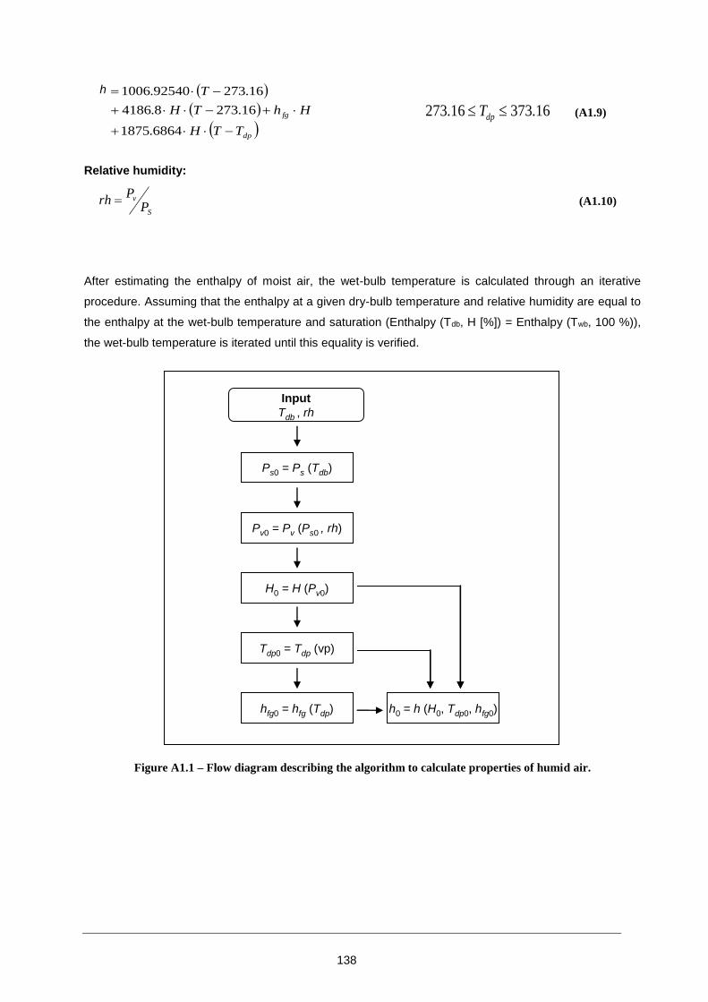
138

h

dp

fg

TTH

HhTH

T

6864.1875

16.2738.4186

16.27392540.1006

16.37316.273 dpT (A1.9)

Relative humidity:

S

v

PP

rh (A1.10)

After estimating the enthalpy of moist air, the wet-bulb temperature is calculated through an iterative

procedure. Assuming that the enthalpy at a given dry-bulb temperature and relative humidity are equal to

the enthalpy at the wet-bulb temperature and saturation (Enthalpy (Tdb, H [%]) = Enthalpy (Twb, 100 %)),

the wet-bulb temperature is iterated until this equality is verified.

Figure A1.1 – Flow diagram describing the algorithm to calculate properties of humid air.

Input

Tdb , rh

Ps0 = Ps (Tdb)

Pv0 = Pv (Ps0 , rh)

H0 = H (Pv0)

Tdp0 = Tdp (vp)

hfg0 = hfg (Tdp) h0 = h (H0, Tdp0, hfg0)

139

Figure A1.2 –Flow diagram describing the algorithm to calculate the wet-bulb temperature of humid air.

)/(1

1)/(

2 Air Dry kgOH kgH MoistAir kgAir Dry kgA

(A1.11)

)/(1)/( 22 Air Dry kgOH kgA Air Moist kgOH kgW (A1.12)

Input

Tdb , rh

h(Tdb , rh) = h(Tdb , 100)

? Tdb = Twb

Y

N

htest = h(Ttest , 100)

Ttest = Tdb - ∆T

htest = h(Tdb , rh)

?

N

Ttest = Ttest - ∆T

Y Output

Twb = Ttest

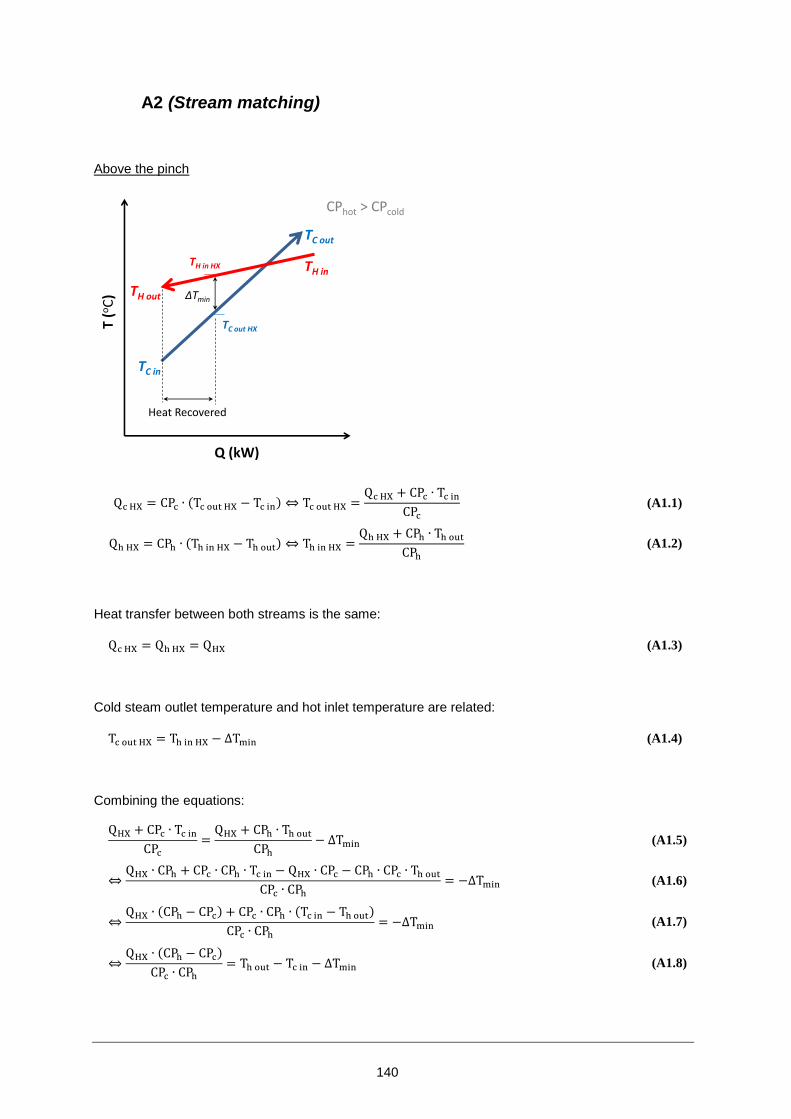
140

A2 (Stream matching)

Above the pinch

Qc HX = CPc ∙ (Tc out HX − Tc in) ⇔ Tc out HX =Qc HX + CPc ∙ Tc in

CPc

(A1.1)

Qh HX = CPh ∙ (Th in HX − Th out) ⇔ Th in HX =Qh HX + CPh ∙ Th out

CPh

(A1.2)

Heat transfer between both streams is the same:

Qc HX = Qh HX = QHX (A1.3)

Cold steam outlet temperature and hot inlet temperature are related:

Tc out HX = Th in HX − ΔTmin (A1.4)

Combining the equations:

QHX + CPc ∙ Tc in

CPc

=QHX + CPh ∙ Th out

CPh

− ΔTmin (A1.5)

⇔QHX ∙ CPh + CPc ∙ CPh ∙ Tc in − QHX ∙ CPc − CPh ∙ CPc ∙ Th out

CPc ∙ CPh

= −ΔTmin (A1.6)

⇔QHX ∙ (CPh − CPc) + CPc ∙ CPh ∙ (Tc in − Th out)

CPc ∙ CPh

= −ΔTmin (A1.7)

⇔QHX ∙ (CPh − CPc)

CPc ∙ CPh

= Th out − Tc in − ΔTmin (A1.8)

Q (kW)

TH in

TH out

TC out

TC in

T (o

C)

Heat Recovered

ΔTmin

TC out HX

CPhot > CPcold

TH in HX

141

⇔ QHX =CPc ∙ CPh ∙ (Th out − Tc in − ΔTmin)

(CPh − CPc) (A1.9)

Below the pinch

Qc HX = CPc ∙ (Tc out − Tc in HX) ⇔ Tc in HX =−Qc HX + CPc ∙ Tc out

CPc

(A1.10)

Qh HX = CPh ∙ (Th in − Th out HX) ⇔ Th out HX =−Qh HX + CPh ∙ Th in

CPh

(A1.11)

Heat transfer between both streams is the same:

Qc HX = Qh HX = QHX (A1.12)

Cold steam inlet temperature and hot outlet temperature are related:

Tc in HX = Th out HX − ΔTmin (A1.13)

Combining the equations:

−QHX + CPc ∙ Tc out

CPc

=−QHX + CPh ∙ Th in

CPh

− ΔTmin (A1.14)

⇔−QHX ∙ CPh + CPc ∙ CPh ∙ Tc out + QHX ∙ CPc − CPh ∙ CPc ∙ Th in

CPc ∙ CPh

= −ΔTmin (A1.15)

⇔QHX ∙ (−CPh + CPc) + CPc ∙ CPh ∙ (Tc out − Th in)

CPc ∙ CPh

= −ΔTmin (A1.16)

⇔QHX ∙ (−CPh + CPc)

CPc ∙ CPh

= Th in − Tc out − ΔTmin (A1.17)

Q (kW)

TH in

TH out

TC out

TC in

T (o

C)

Heat Recovered

ΔTmin

TC in HX

CPhot < CPcold

TH out HX

142

⇔ QHX = −CPc ∙ CPh ∙ (Th in − Tc out − ΔTmin)

(CPh − CPc) (A1.18)

A3 (Stream match tools)

A description of the tool developed for applying the stream match methodology is described herein. The

tools were developed using Microsoft Excel. For applying the methodology three files are used:

Above pinch.xls Used to match the streams above the pinch.

Below pinch.xls Used to match the streams below the pinch.

HX network.xls Used to visualize the heat exchanger network and optimize the temperature

approach.

A3.3.1 Above pinch.xls

1. In the “INPUT” sheet input the data related to each stream namely: Tin [C], Tout [C], FCp [kW.C-1],

Q [kW], HTC [kW.m2.C-1]. In this sheet the hot and cold pinch temperature must also be stated. To

determine the pinch temperature other tool should be used [97].

2. Then “Feasibility matrix”, where 1 represents a feasible match and 0 a non-feasible match.

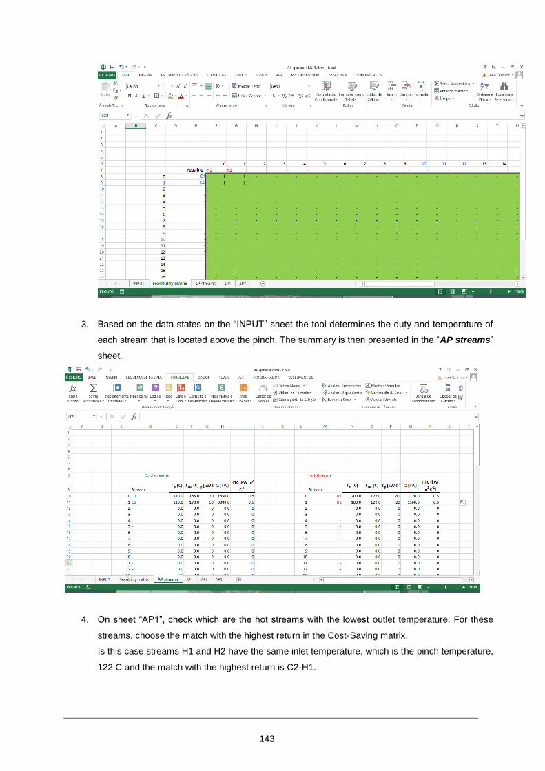
143

3. Based on the data states on the “INPUT” sheet the tool determines the duty and temperature of

each stream that is located above the pinch. The summary is then presented in the “AP streams”

sheet.

4. On sheet “AP1”, check which are the hot streams with the lowest outlet temperature. For these

streams, choose the match with the highest return in the Cost-Saving matrix.

Is this case streams H1 and H2 have the same inlet temperature, which is the pinch temperature,

122 C and the match with the highest return is C2-H1.

144

5. On sheet AP2 select the streams (green box) which were selected in the previous step.

6. On sheet “AP2”, check which are the hot streams with the lowest inlet temperature. For these

streams, choose the match with the highest return in the Cost-Saving matrix.

In this case stream H1 has an inlet temperature of 197 C and stream H2 an outlet temperature of

122 C. Since stream H2 has an outlet temperature lower than stream H1, only this stream will be

considered and the selected match will be C1-H2.

145

7. Copy the last sheet, in this case sheet AP2, and paste it at the end. Change the name of the sheet

so that the sheets have a sequential numeration.

146

8. On sheet AP3 select the streams (green box) which were selected in the previous step.

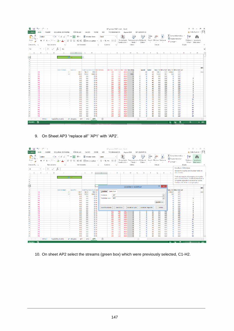
147

9. On Sheet AP3 “replace all” ’AP1’ with ‘AP2’.

10. On sheet AP2 select the streams (green box) which were previously selected, C1-H2.

148

11. Choose the match with the highest return.

12. When no more streams are available to match stop the process.

A3.3.2 Bellow pinch.xls

Follow the same procedure as for the Above Pinch worksheet but in this case the order for choosing the

matches start with the cold streams with the highest outlet temperature and gradually move out of the

pinch.

149

A3.3.3 Pinch Tool.xls

1. Specify the input data in the green boxes

2. Build the network that was determined using the Above Pinch.xls and the Bellow Pinch.xls tools

To insert a new Heat exchanger copy an existent one.

150

,and then insert the copied cells.

3. To insert a new stream follow the same procedure as with the heat exchanger but insert the copies

cells in a row.

151

4. Link the cells that are dependent of each other. For example, the cold outlet of heat exchanger 2

equals the cold inlet of heat exchanger 3

5. The temperatures at the pinch are considered independent variables, so they are explicated in a

group of cells (on the HX network the independent variables are in green).

152

6. Use solver to find the minimum annual cost of the network.

7. Check the network and evaluate the results.

In this case cold utility could be removed.

evaluation and optimization of an industrial utility system

Documents