evaluating virtual options - annual international real options
TRANSCRIPT

Evaluating Virtual Options
Current revision: March 15, 2001
Andrew H. Chen*James A. Conover**
and John W. Kensinger**
*Cox School of BusinessSouthern Methodist University
Dallas, TX 75275
**College of Business AdministrationUniversity of North Texas
P.O. Box 305339Denton, TX 76203-5339
Address correspondence to John Kensinger, or call at:
940-565-2511 (Voice)940-565-4234 (Fax)
For the most recent revision, visithttp://www.coba.unt.edu/firel/Kensinge/papers/virtual.pdf
Alphanumeric Classification System Subject Descriptors:
G310 Capital Budgeting: Investment Policy
G130 Contingent Pricing; Futures Pricing; Option Pricing

1
Evaluating Virtual Options1
Abstract
With virtual options the underlying assets are information and the rules governingexercise are based on the realities of the information realm (infosphere). Virtual optionscan be modeled as options to “purchase” information items by paying the cost of theinformation operations involved. Virtual options arise at several stages of value creation.The initial stage involves observation of physical phenomena with accompanying datacapture. The next refinement is to organize the data into structured databases. Theninformation is selected from storage and synthesizing it into an information product (suchas a report, article, or design specifications for a product to be fabricated in the physicalrealm). Then the information product is presented to the user via an efficient interfacethat does not require the user to be a field expert. Virtual options are similar in conceptto real options but substantially different in their details, since real options have physicalobjects as the underlying assets and the rules governing exercise are based on the realitiesof the physical world. Also, while exercising a financial option typically kills the option,virtual options may include multiple exercise. Virtual options may involve high volatilityor jump processes as well, further enhancing their value. Application of option pricingtheory to real options has yielded worthwhile tools for disciplined decision making, andthe potential also is great for worthwhile decision support tools based upon virtualoptions. This paper extends several important real option applications into theinformation realm, including jump process models and models for valuing options tosynthesize any of n information items into any of m output products.
Introduction
Virtual options involve choices in which the underlying assets are information
items. Transition-phase virtual options accrue as a result of possessing information, and
have real options as the underlying assets. The rules governing exercise of virtual
options are based on realities that exist within the information realm (infosphere). Virtual
options parallel real options in various applications along the value chain; but differ in
their details, since real options have physical objects as the underlying assets and the
rules governing exercise are based on the realities of the physical world.2 Just as real
option applications offer tools for improved decision making for a variety of physical
investments, virtual options offer potential improvements in decision support for those
whose shareholder value results from information operations (including gathering,
storing, processing, or presenting information).
1 The authors appreciate Phelim Boyle’s updated, electronic algorithm supplied from the working paperversion of Boyle/Tse (1990); and the updated, electronic version of the multivariate normal subroutineMULNOR supplied by Mark Schervish.
2 Financial options, from which the models we use are derived, have publicly-traded securities asunderlying assets, and the rules of exercise are set forth in written contracts.

2
Virtual options can be modeled as options to “purchase” information items by
paying the cost of the information operations involved. Virtual options arise at several
stages of value creation, starting with information gathering. This first stage involves
observation of physical phenomena with accompanying data capture. The next stage
involves organizing the data into structured databases. The third stage involves selecting
information from storage and then synthesizing it into an information product (such as a
report, article, or design specifications for a product to be fabricated in the physical
realm). Then the information product is distributed (over information channels) and
presented to the user via an efficient interface that does not require the user to be a field
expert. In the end, the user applies the information in order to add value in the physical
realm. Thus the loop is closed with value added in the physical realm. (Section 2
provides illustrations of virtual options in a sequential decision process.)
There are some important distinctions between virtual options and real options.
First, exercising an option to exchange one set of information in return for another
information item does not involve destruction of the input (in contrast, an option to
convert one physical commodity into another typically involves using up the input good).
So, whereas many real options may be exercised only once, virtual options can have
multiple exercise. Thus a given set of information items may spawn several options that
can be exercised from it, and exercising one of them does not destroy the others.
Therefore the potential value generated by virtual options may be greater than in the case
of real options.
Additionally, options with information items as underlying assets may be more
likely to involve high volatility or jump processes (compared with options that have
physical items as underlying assets). For example, a new discovery might initiate a
substantial jump in the value of virtual options that arise from an organization’s
proprietary information. On the negative side, a discovery by a competitor might
immediately reduce or eliminate the value of options that arise from an organization’s
proprietary information. With the limited liability of options, such substantial movement
potential translates into high option values.
These characteristics of multiple exercise and high volatility could explain
seemingly high market valuations for equity in companies that derive their value from
information operations. Possession of proprietary databases and unique ability to process
information into marketable intellectual property could support equity values that
significantly exceed amounts attributable to physical assets in place or cash flows from
existing physical operations.

3
The literature of real options consistently argues that discounted cash flow (DCF)
calculations underestimate net present value, and attribute the shortfall to DCF’s failure
to consider the value of choice and flexibility. Yet when there have been opportunities to
compare the real options evaluations with market evaluations, the real options approach
also has been found to underestimate value.3 Evaluation of virtual options may help gain
insight into the sources of value that are not being measured by other techniques.
Indeed, real option applications have helped bridge the gap between finance and
strategy.4 Business strategy has roots in military strategy (the word “strategy” derives
from Greek roots meaning “the art of the general”) which opens some interesting issues.
During the 1990s the military leadership in several nations have devoted substantial
resources to information warfare—that is, military actions in which the targets are
information and the avenues of attack are across information channels. The U.S. Joint
Chiefs of Staff have identified “Information Dominance” as one of five basic core
competencies necessary for a modern military force.5 Information warfare is further
differentiated from “information in warfare.” The latter involves using modern
information technology to enhance effectiveness and efficiency of traditional military
activities that involve applying energy to physical targets. Information warfare is
distinctly different in the nature of the targets and the avenues of engagement—some
information warfare specialists refer to themselves as “cyber warriors.”
Similar distinctions can be drawn for business activities. “Information in business”
involves using knowledge to enhance effectiveness and efficiency of business activities
that involve transforming physical objects in order to add value.6 (There are discussions
below summarizing several real option applications that have been developed around the
concept of options to exchange one asset for another, or any of n inputs into any of m
output products.) “Information business” would encompass actions involving businesses
whose shareholder values result from gathering, storing, processing, or presenting
information—those for whom information is product as well as raw material, and
information channels are the route of access and delivery. Virtual option applications can
fill gaps in the analysis of value added by information in traditional business activities.
3 See Brennan and Schwarz (1985), Siegel Smith and Paddock (1987), and Paddock Siegel and Smith(1988).
4 See Amram and Kulatilaka (2000).
5 “Information Dominance” includes the ability to protect and utilize one’s own information resourceswhile denying the enemy the ability to rely upon its information resources.
4
Further, virtual options are uniquely appropriate for analyzing investments in information
business.
1.0 Overview of Real Option Applications, and Virtual OptionParallels
1.1 Abandonment Options
The first applications of option pricing theory to the valuation of real options were
aimed at the option to abandon a project entirely and liquidate its assets.7 Abandonment
options can be evaluated using models for the value of a put option. In the realm of
virtual options where the underlying assets are information items, complete abandonment
may not be a practical issue. When digital information is abandoned, the positive benefit
is measured in terms of storage capacity released for other uses. Given the very low cost
of archiving digital information, there would be little incentive to completely discard any
of it (unless there is concern that it might have negative impact if later discovered, which
involves issues beyond the intended scope of this paper).
1.2 Basic Extraction
Next, real option applications were developed for valuing natural resource
investments such as mines and oil leases.8 Such projects can be viewed as options to buy
basic commodities, and evaluated using the Black-Scholes Option Pricing Model.9 These
activities occur at the beginning of the value chain.10 Rayport and Sviokla (1995) have
translated the physical value chain into its parallel in the information realm. At the base
of the virtual value chain are the activities that involve gathering information by
observing physical phenomena. A simple call option model might be appropriate for
situations in which a single information item can be “purchased” by paying the cost of
observation. This is a limited scenario in the information realm, however. Alternative
6 See for example Feigenbaum, McCorduck, and Nii (1988).
7See Kensinger (1980) and Myers & Majd (1983).
8 Growth options (options to generate new activities that arise from current activities) have also beenpresented in terms of call options, but the identity of the underlying asset is less clear, and so the values forentry into the model are less clear than in the case of natural resource investments
9See Brennan & Schwarz (1985) and Siegel, Smith, & Paddock (1987).
10 See Michael Porter (1985) for a description of the generic value chain.

5
scenarios would include multiple information items captured by a given observation, or a
choice of the most valuable of several information items derived from a given
observation. These possibilities represent more complex options, some of which are
examined later in this paper. Then the decision whether to observe or not could be
evaluated by comparing the value of the acquired option with the cost of observation.
Also, the raw data itself may best be viewed as an option, to which we now turn.
Figure 1: The Physical Value Chain from a Global Perspective
Figure 2: The Virtual Value Chain
1.3 Options to Exchange One Asset for Another
Next in the ascent of real option applications along the physical value chain, options
to exchange one product for another have been applied to gain insight into the value of
conversion processes such as smelters or oil refineries.11 Such options can be evaluated
using the Margrabe (1978) model. The comparable stage in the virtual value chain
involves organizing raw data into databases that facilitate later retrieval (as raw data is
11See Kensinger (1987) and Triantis & Hodder (1990).

6
refined into information, information into knowledge, and knowledge into wisdom).12
Unlike the refining processes in the physical realm, raw data need not be destroyed in the
refining (the raw data may be archived for later use). Thus there is not an exact parallel
between the physical realm and the information realm with regard to refining processes.
Rather, in the information realm, something new is created when raw data is refined,
without damage to inputs. Thus, holding raw data provides the option to purchase
information by paying the price of incorporating it into a structured database.
Further, any given data set may represent multiple options in a package possessing
an admirable quality: unexercised options need not be destroyed in the process of
exercising others. Thus we should proceed to more complex options.
1.4 Multiple Exchange Options
Real option analysis has been applied to activities (such as flexible manufacturing
facilities) that involve transforming the least expensive of several inputs into the most
valuable of several possible outputs. In a move to the parallel position on the virtual
value chain, an organized database (or linked set of multiple databases) provides options
to select information and synthesize it into products such as reports, articles,
documentaries, or books. Synthesis takes place within the infosphere, and people
involved in the process can work from any physical location. The value of organized
data is enhanced because exercise of any option does not destroy other options.
Section 3 presents a discussion of options to exchange the cheapest of several
inputs for the most valuable of several outputs. This discussion begins in terms of
Margrabe’s (1982) generic model, which is broad enough to include a variety of
probability distributions for generating prices. Then the discussion extends to an
implementation using the Boyle-Tse (1990) algorithm for solving the Johnson (1987)
model.
1.5 Remaining Stages of the Virtual Value Chain
The next stage of the virtual value chain described by Rayport and Sviokla (1995)
involves distributing the information product (report, article, design specifications for a
product to be fabricated in the physical realm, etc.). This takes place in the information
realm. Subsequently, the information product is presented to a user. Then in the final
stage of the value chain, the user applies the information in the physical world, perhaps to
12 This statement of the objective of information operations is from Lt. Gen. Michael Hayden, Director ofthe United States National Security Agency.

7
achieve greater effectiveness or efficiency in a physical activity—so here the loop with
the physical world is closed.13.
Thus recapping the virtual value chain and the virtual options represented at each
stage, we start with gathering information. This first stage involves observation of
physical phenomena with accompanying data capture. The second stage involves
organizing the data into structured databases. The next stage involves selecting
information from storage and then synthesizing it into an information product (such as a
report, article, or design specifications for a product to be fabricated in the physical
realm). Then the product is distributed (over information channels) and presented to the
user via an efficient interface that does not require the user to be a field expert. In the
end, the user applies the information successfully to add value in the physical realm.
Thus the loop is closed with value added in the physical realm.
To summarize the virtual options framework, we can then work backward from the
final application. The effort expended in transmitting and presenting the information
product can be evaluated as a decision to exercise an option—the motivation for exercise
is the value added in the physical realm when the information product is applied. This
value added can be evaluated as an option to convert one of n physical inputs into the
most valuable of m physical outputs (without the information, one would not know how
to do this). Backtracking, the price paid for the synthesis effort is defined by the value of
the option just described. Backtracking further, the value of organizing the database is
the value of a portfolio of options to produce information products such as reports,
articles, or design specifications; and the value of raw data is represented by the value of
options to convert it into organized databases.
2.0 Illustration of Real Options and Virtual Options in a SequentialDecision Process
As an illustration of the way virtual option analysis could enhance decision making,
let us consider a sequential decision process at Royal Dutch/Shell that unfolded over a
time period extending more than a decade. The details have been reported in the Wall
Street Journal (for the readers’ convenience, the feature article is included as Appendix
13 The process of adding value in the virtual value chain begins with observation drawn from the physicalworld. It then proceeds to several stages that take place in the infosphere: data is organized, then selected,synthesized, and distributed. Next, it is presented back into the physical realm, and applied to gainenhanced value-added in the physical realm.

8
B).14 The decision process began in May 1985 with the choice of bidding on an offshore
drilling lease in the Gulf of Mexico, dubbed the “Mars” field. Initial survey data had
produced difficult-to-interpret data that some thought might indicate oil deposits. After
winning the lease, the next choice involved exploratory drilling. The affirmative decision
here resulted in discovery of a so-called “elephant” field; but the decision process did not
end, because the site was so deep underwater. The next choice involved innovating new
drilling technologies capable of developing the site. Once the technology was in hand,
the final choice was when to proceed with development.
The decision process begins with Shell’s efforts to map the region in preparation for
the auction of drilling rights by the federal government. (The saga begins at a time when
capital markets were apparently discouraging major expenditures for exploration.)
Geologist Roger Baker encountered many difficulties interpreting the seismic data
because of distortions produced as the signals passed through the thermal layers
encountered in the deep water (such thermal layers act as lenses, but it is difficult to
know how the signals are being distorted). Despite these difficulties, the company had to
decide whether (and how much) to bid on the site. One can approach the problem of
valuing oil leases by treating such leases as call options.15 Greater upside potential, of
course, translates into higher option value. (In sealed bidding Shell paid $2.4 million for
the rights to drill, a 37% premium above the minimum allowable bid, with no other
company making a competing offer).
The next step in the decision process involved exploratory drilling, which cost $14
million. In part, it could be justified as a means for improving the knowledge necessary
to decide optimal exercise of the real option identified above. (From this point of view
the question focuses on the role of the new information in improving the ability to
evaluate the option to develop the site.) In addition to learning what resources might lie
in this specific deposit, however, potentially valuable lessons could be learned from
comparing actual drilling data with the seismic data gathered in the initial survey. Such
lessons might give Shell some competitive advantages in interpreting preliminary data on
new fields to be considered in the future.
How could we evaluate lessons learned concerning interpretation of seismic data
from deep-water prospecting in general? Royal Dutch/Shell would have knowledge
about similar information from other locations in its proprietary databases. Learning the
14 Solomon and Fritsch (1996).
15 For details on this application, see Siegel, Smith, and Paddock (1987).

9
truth about the Mars site could substantially enhance the value of such information. A
positive outcome would identify new development options of the Siegel/Smith/Paddock
variety for each such similar location (and a negative outcome here could prevent losses
elsewhere). Knowing the number of similar sites in its databases, Royal Dutch/Shell
could tally the options potentially available to it. The transition-phase virtual option
associated with the exploratory drilling at the Mars site has this portfolio of real options
as the underlying asset. Given the global scope of Royal Dutch/Shell seismic data-
gathering activities, this virtual option could have substantial upside potential (hence
substantial value, due to the limited downside risk).
The exploratory drilling revealed that the Mars field contains 700 million barrels of
oil, the biggest domestic discovery since Alaska’s Prudhoe Bay. (This is about one-third
the size of all Gulf Oil Company’s recoverable reserves at the time of its merger with
Chevron.) Shell’s problem was that no one had yet gained experience constructing a
production platform capable of operating in such deep water and also capable of
withstanding the hurricanes that occur there. The next part of the decision process
involves a multi-year research effort to design a platform.
How do we evaluate the investment in research devoted to platform design? At the
outset, no one knew for sure whether a successful design could be achieved with
available technology, or whether a production platform could be built at a cost that would
make developing the field economically viable. Strictly within the confines of the Mars
field, we are still dealing with the Siegel/Smith/Paddock real option that has developed
reserves as the underlying asset. The exercise price of this option is uncertain at this
stage of the decision process, and the proposed research would provide new information
to enlighten the evaluation of this real option.
Also, however, proprietary knowledge gained from platform development efforts
could be valuable in other future applications. A positive outcome could create new
development options that would accrue from information about other similar deep-water
sites known from Royal Dutch/Shell’s proprietary databases of seismic observations.
When the research into platform design was complete, Shell had the task of
evaluating the expenditure of $1.1 billion to build a platform and drill 26 production
wells (this is about $1.57 per barrel). The platform would cost $650 million and the
drilling would cost another $450 million. Some of this cost would be shared with
minority partner British Petroleum. The expenditures at this stage would be the largest in
the whole development effort. Although this is the stage in the decision process that
involves the most money, it is the least complex. The remaining decision is whether to
exercise the real option to pay drilling costs and receive the developed reserves. At this

10
stage there is highly refined information about the exercise price and about the value of
the underlying asset, so the decision process can proceed smoothly.
2.1 Virtual Options in Basic Research
What about the expense of Roger Baker’s initial efforts gathering information—the
basic research that gave rise to the entire process we have just reviewed? Also, how does
the new knowledge about interpreting deep-water seismic observations affect the value of
future survey efforts?
In a mature information culture new data gathering tends to occur at the frontiers of
available knowledge. When Roger Baker, for example, gathered his survey data, he
applied existing methods for exploring in a new area. Roger Baker is a prospector with
experience about the probability of discovery from a given search effort. This probability
distribution could be treated as the underlying stochastic process in evaluating the effort
as a virtual option (the underlying asset being information of value for use in bidding on a
lease).
Interpreting Roger Baker’s data proved challenging for unforeseen but
understandable interference by the thermal layers in the deep water. Subsequent
clarification of how to interpret this data could produce benefits in at least two ways.
First, the newly acquired skill could be applied to data produced in prior deep-water
surveys at other locations, with new drilling options as the result (as discussed above).
Further, the new capability to interpret data changes the probability of discovery from
future survey efforts, thus encouraging future prospecting.
2.2 Virtual Options in Human Resources Development
Investments in human resources development may alter the exercise price of an
organization’s virtual options. Improved engineering capabilities, for example, may
reduce the exercise price for an option to derive product designs from proprietary data.
Analyzing the impact on the value of an organization’s virtual options therefore could
provide useful insights for decisions about investments in human resources development.
Beech Aircraft Company provides an example. Brand identity was strong, with a
solid reputation for product quality; but the existing product line was dominated by aging
designs. In 1979 Beech committed to developing a revolutionary design (dubbed
“Starship”) that used all-composite construction, fully computerized flight instruments,
jet-fan power, and the then-radical canard architecture (on a canard aircraft, the main
lifting wing is at the rear, with the horizontal stabilizer mounted on the nose). Most of
the investment went into computer-aided design facilities and factory automation for

11
handling composite materials on a large scale (which have many alternative uses, hence
generating valuable real options). This effort attracted new engineering talent and
revitalized the company to such an extent that Beech attracted significant attention as a
strategic acquisition with several potential suitors. (Beech’s primary stockholder at the
time was the founder’s widow, who wanted to retire and had significant estate-planning
issues.) The result was a successful sale to Raytheon within less than a year of launching
the Starship project, nearly doubling the value of Beech stock in four months. (Raytheon
was the primary supplier of cockpit instruments, communications equipment, and
navigation aids for the Starship project).
The Starship itself had a very brief production run, but the capabilities developed
during that effort have enhanced the organization in a variety of ways. Chief among the
gains achieved through the Starship program was the enhanced ability to attract and
retain high-quality engineering talent.16 With the engineering talent, computer-assisted
design, and computer-integrated manufacturing systems established via the Starship
development program, Beech substantially reduced the cost of developing new product
designs and improvements for existing products. Highly visible among the new products
that resulted is a new jet aircraft with aluminum wings and composite fuselage. Beech’s
design and composite materials production capabilities have also resulted in several
contracts to supply components for other manufacturers (including parts for the B-2
bomber and the C-17 cargo aircraft built for the U.S. Air Force). These capabilities
directly result from the investments made in the Starship program.
3. Models for Evaluating Virtual Options
3.1. Jump Process Model
In order to evaluate virtual options, let us begin with the case of a single input and
single output, with the possibility for discontinuous jumps in value. Options with
information items as underlying assets may be more likely to involve high volatility or
jump processes (compared with options that have physical items as underlying assets).
For example, a new discovery might initiate a substantial jump in the value of virtual
options that arise from an organization’s proprietary information. On the negative side, a
discovery by a competitor might immediately reduce or eliminate the value of options
that arise from an organization’s proprietary information. This section presents a general
16 The author learned this in an interview with a Beech executive who wishes to remain anonymous.
12
valuation model for virtual options with underlying stochastic process described as a
mixture of both jump and diffusion processes.
When the virtual option can be exercised without destroying the input information
items, then complex options can usually be represented as portfolios of several options,
each one conveying the privilege to generate a single output item. For each of these
individual options, the total change in the value of the underlying asset is assumed to
consist of two types of changes:
(1) The small and “normal” changes in the market value of the firm that are
modeled as Brownian motion with a constant variance per unit time and a
continuous sample path.
(2) The large and “abnormal” changes in value that are due to arrival of
significant unanticipated events.
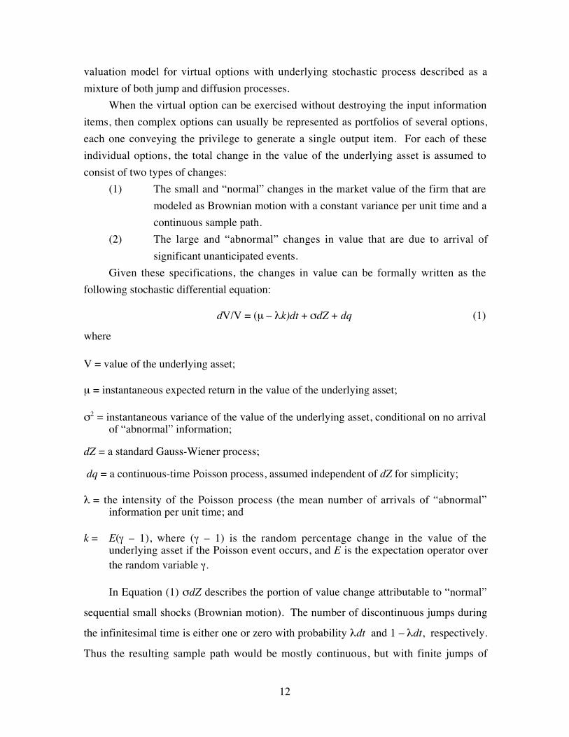
Given these specifications, the changes in value can be formally written as the
following stochastic differential equation:
dV/V = (µ – λk)dt + σdZ + dq (1)
where
V = value of the underlying asset;
µ = instantaneous expected return in the value of the underlying asset;
σ2 = instantaneous variance of the value of the underlying asset, conditional on no arrivalof “abnormal” information;
dZ = a standard Gauss-Wiener process;
dq = a continuous-time Poisson process, assumed independent of dZ for simplicity;
λ = the intensity of the Poisson process (the mean number of arrivals of “abnormal”information per unit time; and
k = E(γ – 1), where (γ – 1) is the random percentage change in the value of theunderlying asset if the Poisson event occurs, and E is the expectation operator overthe random variable γ.
In Equation (1) σdZ describes the portion of value change attributable to “normal”
sequential small shocks (Brownian motion). The number of discontinuous jumps during
the infinitesimal time is either one or zero with probability λdt and 1 – λdt, respectively.
Thus the resulting sample path would be mostly continuous, but with finite jumps of

13
differing signs and amplitudes at discrete points. Given V(0) = V and µ, λ, k and σ are
constants, the random value of the underlying asset at time t can be expressed as
V(t ) = V exp [(µ – σ2/2 – λk)t + σZ(t )] γ(n ) (2)
Where Z(t) is a Gaussian standard normal random variable with zero mean, γ(n ) = 1 if n
= 0; γ(n ) = ΠNj=1 γj for n ≥ 1 where γj are the jump amplitudes assumed for simplicity to
be independently and identically distributed and n is Poisson distributed with parameter
λt.
Under the assumptions that the capital asset pricing model (CAPM) holds and that
the jump process is diversifiable, Merton (1976) shows that the price of any contingent
claim, F(V,t) which is a function of the value of the underlying asset and time must
satisfy the following general valuation equation:
.5σ2V2Fvv(V,t) + ( r – λk )VFv(V,t) + Ft(V,t) – – rF(V,t) + λE(F(VY,t) – F(V,t )) = 0 (3)
which is an integro-differential equation where the expectation is taken over the random
value of the jump amplitude γ, and r is the constant instantaneous riskless rate of interest.
The unique fvalue of the contingent claim on the underlying asset is determined by the
initial and boundary conditions (which generally include F(0,t) = 0 and F(V,t) ≤ V ).
Additional boundaries can be stated when required by the constraints of specific
situations.17
Note to program committee: The authors plan to explore possible boundary conditions
more fully in future revisions.
3.2. Multiple Outputs, Choice of Inputs
In the case of multiple outputs (OUT1, … , OUTn), but only one input (IN ), the end-
of-period payoff can be represented by the following expression:
Payoff = Max {Max [OUT1, … , OUTn] – IN, 0} (4)
That is, at the time the decision is made about how to use the information in a given
time period, the output with maximum value will be chosen; and the payoff will be the
difference between the value of that output and the cost of the input.
17 See Merton (1976) for further discussion of boundary conditions and valuation procedure.

14
In the case of more versatile information processing systems, the option-holder has
the choice in each time period to convert the lowest cost input from a set of m inputs into
the highest valued output from a set of n output items, but need not exercise the option
unless it is profitable to do so (a binomial illustration and numerical examples are given
in Appendix A). The value of this option at any time prior to the expiration date can be
solved numerically, using techniques developed by Margrabe (1982) for situations that do
not involve discontinuous jumps. This scenario can be represented more compactly by
supposing that the current prices at time t for the various information items form a
vector, x = x1,L, xn[ ], the prices at future time T form a vector X = X1,L, Xn[ ], and q(…) is
a multivariate p.d.f. for the vectorX, given the initial set of current prices at time zero (the
vectorx.). The production of information outputs from the raw input can be represented
by some function f(X)..18 This function could be simple or quite complex. The interest
rate is r for US Treasury securities maturing at time T. Then, the value of an option to
accomplish the optimal transformation is given by the following:
Option Value = e–r(T-t) ∫ … ∫ f(X) q(X,Τx) dx (5)
where integration is over the n- dimensional array of future prices for all of the
commodities. Margrabe proved this solution for the case of a log-Gaussian
p.d.f.—showing that the richer the array of choices, the higher the NPV of the project.
The virtual option package is a portfolio of the above options with different
maturities, with one maturing in each period of the project’s life.
3.3 Implemention Using the Boyle and Tse Algorithm
Johnson’s (1987) model calculates the exact value of a call option with exercise
price X and time to maturity T, on the maximum of N assets with current values S1, S2,…,
Sn. Computing the exact solution requires numerically evaluating N +1 N-dimensional
standard normal distribution functions. This is practical for N <6 on personal computers
using the Schervish (1985) algorithm. Solving with N =6 is practical only on
minicomputers and mainframes, while N >6 is practical only on super computers.
Chen, Conover, and Kensinger (1998) have implemented the multiple exchange
option framework using the Boyle-Tse (1990) algorithm for evaluating an option on the
maximum or minimum of several assets. This algorithm has overcome earlier criticism
that realistic problems could not be solved without consuming large amounts of computer
18For example, f X( ) = Max 0, X2 − X1( ) .

15
time (the program is available from the authors upon request). Chen, Conover, and
Kensinger report the ability to solve problems with up to 1,000 different output goods at
high speed on a personal computer with a math coprocessor, and have solved problems
with up to 9,000 output goods in about 30 seconds on a 250 Megaherz Sun SPARC
workstation.
The Boyle/Tse (1990) formulation can be applied to a wide range of problems that
used to be too costly (or impossible) to evaluate. Detailed description of the steps is too
lengthy for this paper, but a copy of the computer code is available upon request. What
follows is a description of the principle steps of the algorithm. First, the N assets are
assumed to be jointly multivariate normal. Direct evaluation of the multivariate normal
distribution function is very costly for N >6, but the maximum of two bivariate normally-
distributed assets is well defined. The algorithm uses a recursive technique that
successively compares N assets, taken two at a time. Let us begin by assuming that
MAX x1, x2( ) is normally distributed. Given this assumption, the expected value, variance,
and covariance of MAX x1, x2 , x3( ) can be approximated using the recursive relationship:
MAX x1, x2 , x3( ) = MAX MAX x1, x2( ), x3( ) (6)
Then, the first four moments of the maximum of the first three assets with the fourth are
calculated using:
MAX x1, x2 , x3, x4( ) = MAX MAX x1, x2 , x3( ), x4( ) (7)
Repeatedly applying this procedure to the remainder of N variables (using the current
cumulative maximum value at each step) allows approximation of the distribution of the
maximum of N jointly random normal variables.
Zero strike options on lognormally-distributed assets are examined by discounting
(under risk neutrality) the expected value of the log of the maximum of N asset prices.
For non-zero strike prices the procedure estimates the probability that the maximum of N
assets will exceed the strike price of the option. First, the recursive algorithm described
above is used to calculate the first four central moments of MAX x1, x2 ,K, xN( ). The second
step is to form a Taylor series expansion of the option pricing problem using the
standardization transform in terms of the first four central moments of the maximum of N
jointly multivariate normals from the first step. A Gram-Charlier expansion of the
Taylor-series is solved to calculate the probability that MAX x1, x2 ,K, xN( ) will be greater
than the exercise price.

16
The algorithm described in Boyle/Tse (1990) is an accurate approximation that is
fast enough to run on a personal computer. For N up to 50 assets, the approximation
error is as low as 0.06 percent. The algorithm has four appealing characteristics:
• It requires only the evaluation of univariate normal distributions that are simpleand inexpensive to perform.
• The algorithm runs very quickly compared to its only competitor, which isrepeated simulation sampling.
• The algorithm is very accurate over a wide range of the parameters.
• The model predictions can be checked against independent estimates of the modelprices from Monte Carlo sampling of multivariate distribution functions or directevaluation of the distribution functions.
In simulation trials to evaluate how value responds to increasing flexibility, Chen,
Conover, and Kensinger (1998) report results similar to those observed in diversified
portfolios of securities. At first, additional outputs or inputs add substantially to value,
but after twelve to fifteen alternatives are already available, more new alternatives add
very little additional value.
3.4 Estimating the Covariance Matrix
The virtual option approach requires two types of data: (1) current values for the
information items involved, and (2) the descriptions of the probability distributions that
generate future values. The current prices themselves may be directly observable or
readily proxied. Let us now consider the estimation of parameters for the covariance
matrix.
In the Johnson model, and the Boyle and Tse implementation, each of the n asset
prices, n standard deviations and the nxn correlation matrix of each asset with the other
assets must be specified. The model is very sensitive to any errors that might occur in
estimating the covariance matrix.
Option models that capture the value of a simple option on a single asset, such as
Black-Scholes (1973), specify the underlying stochastic process generating returns on the
asset simply in terms of the asset’s total variability (including both systematic and
unsystematic risk combined into one measure). Options to exchange one asset for
another, such as Margrabe (1978), specify the underlying stochastic process in terms of
the ratio of the prices of the two assets (thus the covariance of the two assets enters the
calculation). Multiple exchange options are much more complex and demand careful
estimation of the parameters input into the model. In well-functioning financial markets,

17
asset prices move together when the assets are close substitutes (otherwise there would be
arbitrage opportunities). This characteristic is captured in a carefully-estimated
covariance matrix, or in a diagonal-model approximation such as the capital asset pricing
model in which variability is partitioned into systematic and unsystematic components.
In order to apply the financial markets model successfully to real options or virtual
options, it is necessary to insure that the variance-covariance matrix adequately captures
the webwork of interrelationships among the prices for the input and output items.19
The problem can be illustrated by considering a binomial example based on a series
of coin tosses, such as the illustration in Appendix A. The Johnson model is essentially
an extension of such a binomial process to a very large number of coin tosses spanning
the life of the option. The problem arises because there is no constraint that eliminates
the possibility for one of the output prices to be inflated by a series of “heads” in the
sequence of random coin tosses. When there are a hundred or more output items
involved, the odds are high that within the model, one of the prices will become very
large, thus inflating the calculated value of the option beyond the bounds of reason.
If inputs and outputs were all publicly traded commodities, economic forces of
supply and demand would prevent the price of any one of the output items from rising
well beyond the others over time. One of the output items might rise substantially over a
short time, but producers would increase their output of it, while reducing output of the
others. Price adjustments would follow, so that the whole group of related goods would
remain clustered (although relative prices would be free to fluctuate substantially within
the bounds of the cluster). Chen, Conover, and Kensinger (1998) resolve this problem by
defining the underlying stochastic processes using a linear model similar to the Capital
Asset Pricing Model, in which the are two components defining variability: one
component affects all the items in the matrix, while the other component represents the
unique shocks specific to the individual items.
The values the analyst must estimate, then, are the current prices of the output
items, annualized standard deviations for changes in their values, and the correlation
matrix among them. No forecasting of future prices is necessary (such forecasts, in
contrast, are the essence of discounted cash flow analysis).
19 Chen, Conover, and Kensinger (1998) discovered during simulation trials of the Boyle/Tse algorithmthat the result is very sensitive to any lapses in this regard, rapidly converging toward undefined highvalues if the systematic linkage is inadequately captured. The intuition behind this problem is fairly clear.Without explicit linkage, as the number of inputs and outputs increases, there is an increasing probabilitythat at least one of the several inputs will drop to a low price, while one of the outputs will rise to a highprice.

18
Maintaining consistency in the estimates that are input into the model, and insuring
appropriate structure of the correlation matrix, can be made a function of the software
used to incorporate the exchange option models into decision-support systems.
Programmers will find interesting opportunities to provide expert assistants that will quiz
users, prompting them to think clearly through the underlying strategic issues.
4. Ways in Which the Virtual Option Approach Integrates Financeand Strategy
4.1 Links with the Physical Value Chain
The concept of the physical value chain, presented in Porter (1985), is a useful
reference for assessing the progress that has been made up to now toward integrating
finance and strategy by means of applying option pricing methodologies (see Figure 1
above for a graphic image). On a global scale, extraction or cultivation of basic
commodities is at the bottom of the physical value chain. The second tier involves
processing basic commodities into refined products. Next comes the fabrication of
finished products. At the high end of the physical value chain come the distribution and
marketing of products, and post-sales servicing of customers. Thus the early commodity
option applications, such as Brennan & Schwarz (1985), deal with projects at the low end
of the value chain. Over time the real options literature has extended the commodity
option theme to the valuation of options to exchange a group of commodities for another.
Thus real option pricing applications have extended to higher levels of the physical value
chain—to the physical processing of commodities into refined products, and then to
flexible production systems used in fabricating complex products. Work also continues
to develop real option methods for evaluating activities at the upper end of the physical
value chain: involving distribution, marketing, and service. Real option applications in
evaluating support activities such as technology development or human resources
development have been problematic.20
Evaluating virtual options fills important gaps by applying option analysis to
activities that add value along the virtual value chain. Also, evaluating virtual options
provides new insight into the value of efforts to develop technology or human resources.
This approach may also yield insights in evaluating efforts to improve logistics or service
in the physical realm (such efforts might be analyzed as transition-phase virtual options).
20 See Amram and Kulatilaka (2000) for a discussion of appropriate tools for evaluating investments in

19
4.2 The Knowledge Advantage
There are several additional ways in which the virtual option approach integrates
financial analysis with strategic analysis. Let’s begin with the end-of-period payoff for
the simple case of a single input and a choice among multiple output items, given above
in Equation 4 and reproduced below as Equation 8.
Payoff = Max {Max [OUT1, … , OUTn] – IN, 0} (8)
It can be shown that this dominates an option that includes a smaller set of output items,
such as one with the following payoff:
Payoff = Max {Max [OUT1, … , OUTn-1] – IN, 0} (9)
To demonstrate this point, we compare an option which includes two output items
with another that includes those same outputs plus one more, and find that the three-
output option is worth more because its payoff would be greater in those states of the
world in which OUT3>IN, OUT3>OUT2, and OUT3>OUT1. Therefore, we can state the
following:
An organization that has the same potential uses for a given information item asanother organization, plus one or more additional possible uses unique to thatorganization, will gain a higher NPV by gathering the information. Thus, thevalue of obtaining information may differ from one organization to another, andorganizations with more agility have an advantage in generating investor value.
A well-known property of such options, whether or not the p.d.f. is log-Gaussian, is
that prior to expiration they are worth more than the present value of the spread expected
at expiration (expected price of output minus expected price of input. This can be
illustrated in the simple case of a single output and a single input (the argument is easily
extended to the case of multiple outputs or inputs). At any given time prior to the
expiration of the option,
CX OUT , IN, t( ) > e−rt E OUTt[ ] − E INt[ ]( ) (10)
With the values of the input and output items fluctuating at random, the spread
between them is free to widen or shrink. The existence of discretion allows management
to take whatever profit opportunities arise when the spread is wide, but cut off losses that
would occur when the spread becomes negative. The more volatile the spread, the
greater are the possible profits. Since losses are limited, however, the increased upside
potential is not offset on the downside. The model therefore supports another point:
technology development.
20
The more volatile the relationship between the values of input and output items,the greater the value of a virtual option.
The more volatile each item’s price, and the lower the correlation between their
prices, the more volatile the spread. Therefore, the highest option values are to be found
when values of input and output are volatile, with low correlation. If there were a great
many organizations engaged in the same information operations, competition among
them would tend to keep the spread from fluctuating widely, and output values would be
highly correlated with the input values. A low correlation would be associated with a
situation in which competition is not intense. (A few years ago, for example, DuPont
possessed patents that protected its capability to convert petroleum into a manmade
substitute for wool (polyester), which gave it a significant competitive advantage for a
time. As the capability diffused throughout the economy, however, the advantage
dissipated.) Therefore, the model supports another point:
The value of a virtual option is greater the more innovative the informationoperation, and the stronger the barriers to entry for potential competitors.
This statement is very similar to the lessons derived from a qualitative analysis of
anecdotal evidence by Shapiro (1986) and Porter (1985). The process of estimating the
matrix of correlations in a virtual option evaluation, therefore, entails a quantification of
knowledge structure in the industry. This dimension is not made explicit in the DCF
approach or the real options approach to management.
5. Concluding Remarks
This paper develops the concept of virtual options for inclusion with real options in
capital investment applications. Virtual options involve choices in which the underlying
assets are information items, and the rules governing exercise are based on realities that
exist within the information realm (infosphere). Virtual options differ from real options,
since real options have physical objects as the underlying assets and the rules governing
exercise are based on the realities of the physical world. Transition-phase virtual options
accrue to the owner as a result of possessing information, and have real options as the
underlying assets (transition-phase virtual options capture value at the interface where
information is applied to gain advantage in the physical domain).
The virtual options concept gains structure from the “virtual value chain” described
by Rayport and Sviokla (1995). This traces the process of adding value through
information operations. The first stage involves gathering information from the physical
realm. The next stage involves organizing the raw data into structured databases for later

21
retrieval. The next stage of information operations involves selecting information from
the databases and organizing it into a product such as a report, article, or design
specifications for a product to be fabricated in the physical realm. Then follows
distribution, then presentation to the user. Effective presentation may be challenging, if
the information product is presented to a decision-maker who is not an expert in the field.
Substantial value may hinge on how effectively and efficiently the information is
conveyed to someone who lacks understanding of the basic principles that are part of an
expert’s daily working knowledge. The final stage of the virtual value chain involves
applying the information to gain advantage in the physical realm (this is the stage at
which we encounter transition-phase virtual options). Some stages in the virtual value
chain may be skipped; particularly if the person who develops an information product is
also the decision-maker, in which case the distribution and presentation stages can be
skipped.
Virtual options may exist at each step from one stage of the virtual value chain to
the next. Virtual options can be modeled as options to “purchase” information items by
paying the cost of the information operations involved. The process of gathering raw
data by observations in the physical realm, for example, generates options to organize the
data by paying the cost of populating an existing database or constructing a new one.
Additionally, possessing the necessary organized databases generates options to develop
information products such as design specifications for a product to be fabricated in the
physical realm. Some information operations can be automated, and doing so reduces the
cost of exercise for the information options an organization possesses. Thus the
investment in data automation can be evaluated by measuring the change in value of the
organization’s portfolio of virtual options.
Virtual options can be modeled as options to exchange an input such as an
engineer’s time for an output item that incorporates added value. More often, there may
be a choice of the most valuable among two or more output items; and there may be
possibilities for choosing the least costly of two or more input items (such as when the
input information is purchased). The basic research on options with multiple underlying
assets has been done by Margrabe (1978 & 1983), Stulz (1982), Stulz & Johnson (1985),
and Johnson (1987). Chen, Conover, and Kensinger (1998) applied this method to
evaluating real options associated with flexible manufacturing facilities.
The benefit of evaluating virtual options is not only a more robust set of
quantitative tools for measuring the economic value added by an organized activity, but
also refined insight into the qualitative aspects of a positive net present value action. By
evaluating virtual options along with real options, it is possible to draw well-founded

22
conclusions about the effects on share value of such attributes as flexibility,
innovativeness, and proprietary knowledge. An organization that possesses knowledge
no one else has, for example, has exclusive possession of options to apply it for
advantage in the physical world. Additionally an organization with unique capability to
use information (in a way no other organization can duplicate) has enhanced value
through possessing a broader array of choices.
The concept of the physical value chain, presented in Porter (1985), is a useful
reference for assessing the progress that has been made toward integrating finance and
strategy by means of applying option pricing methodologies. The real options literature
has extended the concept of options to exchange one commodity for another (or one of
several inputs for one of several outputs) to develop real option applications for basic
extraction, refining, and flexible production systems used in fabricating complex
products. Work also continues toward developing real option methods for evaluating
activities at the upper end of the physical value chain: involving distribution, marketing,
and service. Real option applications in evaluating support activities such as technology
development or human resources development have been problematic.21
Evaluating virtual options fills important gaps by applying option analysis to
activities that add value along the virtual value chain. Also, evaluating virtual options
provides new insight into the value of efforts to develop technology or human resources.
This approach may also yield insights in evaluating efforts to improve logistics or service
in the physical realm (such efforts might be analyzed as transition-phase virtual options).
The proposed option techniques surpass the power of complex simulations.
Contingency tables and dynamic programming might be used instead, but the option
approach can be more efficient as well as more powerful. The more complex models
require solution by numerical integration, which of course can’t be done with a simple
hand-held calculator (as can the standard discounted cash flow procedures). The
powerful computers that are now widely available to decision-makers, however, make it
possible to offer complex project evaluation techniques to practitioners in versatile
packages with “smart” interactive interfaces.
21 See Amram and Kulatilaka (2000) for a discussion of appropriate tools for evaluating investments intechnology development.
23
Appendix A: Illustrations and Examples of Option Evaluation
The Option to Exchange One Asset for Another
Here, the investment is formulated as a portfolio of options to exchange a single
input for a single output. In this case the option buyer acquires the opportunity, if it is
profitable to do so in the short run, to purchase the input, convert it, and sell the output
(or do nothing). Moreover, the option holder has a portfolio of such options with
different maturities--one for each time period in the activity’s life.
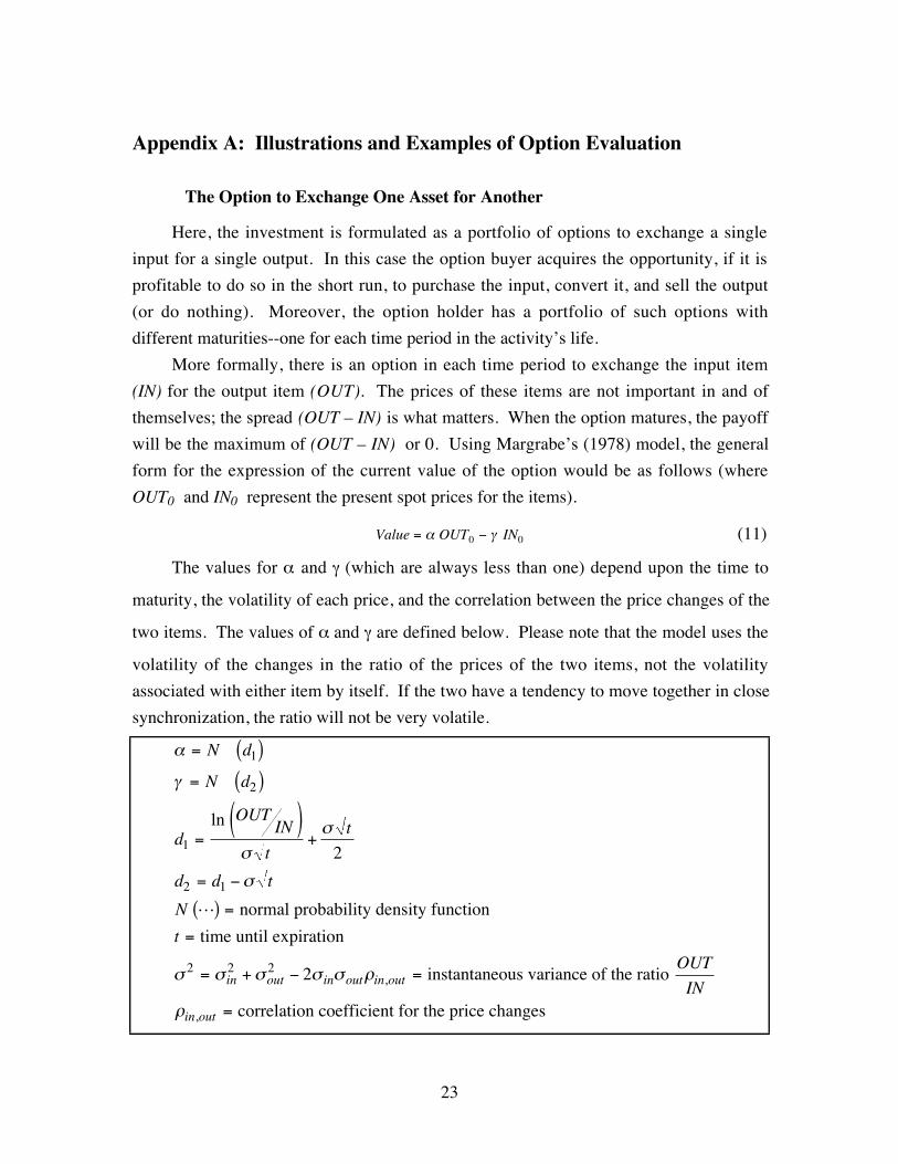
More formally, there is an option in each time period to exchange the input item
(IN) for the output item (OUT). The prices of these items are not important in and of
themselves; the spread (OUT – IN) is what matters. When the option matures, the payoff
will be the maximum of (OUT – IN) or 0. Using Margrabe’s (1978) model, the general
form for the expression of the current value of the option would be as follows (where
OUT0 and IN0 represent the present spot prices for the items).
Value = α OUT0 − γ IN0 (11)
The values for α and γ (which are always less than one) depend upon the time to
maturity, the volatility of each price, and the correlation between the price changes of the
two items. The values of α and γ are defined below. Please note that the model uses the
volatility of the changes in the ratio of the prices of the two items, not the volatility
associated with either item by itself. If the two have a tendency to move together in close
synchronization, the ratio will not be very volatile.
α
γ
σσ
σ
σ σ σ σ σ ρ
ρ
= ( )= ( )
=( )
+
= −
( ) =
=
= + − =
=
N d
N d
d
OUTIN
t
t
d d t
N
t
OUT
INin out in out in out
in out
1
2
1
2 1
2 2 2
2
2
ln
,
,
L normal probability density function
time until expiration
instantaneous variance of the ratio
correlation coefficient for the price changes

24
The net present value of a portfolio of such options, with one of them maturing in
each period of the activity’s life (and with an initial cost of C0 ) could be represented as
follows:
NPV C OUT IN OUT INn n= − + −( ) + + −( )0 1 0 1 0 0 0α γ α γL (12)
The subscripts for α and γ represent the option’s maturity date. This reduces to a
function of the initial cost and the current spot prices of the commodities, as follows:
NPV C OUT INii
n
ii
n= − + −
= =∑ ∑0 0
10
1α γ (13)
A more general form for the solution to the value of each of the individual options
is the following:
CX OUT , IN, t( ) = e−rt E Max OUT − IN, 0( )[ ]= e−rt f OUT , IN( )q∫∫ OUT , IN( ) ∂OUT ∂IN
(14)
where:
r = the appropriate discount rate, usually the riskless rate
E = expectations operator
f OUT , IN( ) = Max OUT − IN, 0( )q OUT , IN( ) = bivariate probability density function
This can be solved numerically, for a variety of probability distributions. In the
case of an asset with a multi-period life, the value of the asset could be represented as a
portfolio of such options, one of which matures at the end of each period.
Contingency Table Example
To illustrate, let us look at a simple numerical example. Consider a scenario
involving a simple binomial probability distribution. We’ll assume that the output item
(OUT) is currently priced at $50, and the input item (IN) is currently priced at $49 (in
time period zero). At the end of time period one (t1), the price of the output will be
determined by the flip of a coin. Heads, the price rises by $1; tails, it falls by $1. A
second coin toss with the same rules will decide the price for the input. At the end of
time period two (t2), another round of coin tossing will take place, with the same rules.
Note that in this very simplified illustration, the price movements of the two items are
assumed to be independent (that is, there is assumed to be no correlation between the
price changes for the two commodities). After this initial illustration there is an example
which uses a modification of the Black-Scholes Option Pricing Model, and at that point
we will consider a more realistic situation.

25
The possible pairs of input and output prices at the end of the first time period are
given on the first line of Table 1. On the second line is the difference (OUT – IN), which
represents the profit from blindly converting the input into the output. With active
management, however, the conversion would not be made if a loss would result; and the
third line shows the profit per unit associated with each outcome when there is active
management.
Place Table 1 about here.
Suppose, for example, we have the opportunity to launch an activity for $2,000,
which has a two-period life, zero salvage value, and the capacity to convert 1,000 units of
the input into 1,000 units of the output. We will ignore taxes. Then, we would use the
average prices for the input and output items to compute the expected net present value.
Since the expected price for the output in each time period is $50 per unit, the expected
price for the input is $49, and volume is 1,000 units, the expected profit in each period is
$1,000 and the expected NPV is the following:22
NPV = −$2, 000 +$1, 000
1.1+
$1, 000
1.12 = −$264.46 (15)
If we recognize the value of the options, however, the expected net present value
changes to the following:
NPV = −$2, 000 +$1,250
1.1+
$1, 437.50
1.12 = $324.38 (16)
The difference is due entirely to the expected present value of the savings produced
by active management. In the first period, there is a 25% probability that the operation
would be suspended, avoiding a loss of $1 per unit. In the second period, there is a 25%
probability of saving $1 per unit, as well as a 6.25% probability of saving $3 per unit.
The present value of these savings sums to the following:
Difference =14
×$1, 000
1.1
+
14
×$1, 000
1.12
+
116
×$3, 000
1.12
= $588.84 (17)
Adding this to the figure calculated with the standard approach yields the true NPV
(that is, $588.84 - $264.46 = $324.38). Thus, some activities that appear to have a
negative NPV when analyzed by traditional DCF methods may actually have positive
NPVs.
22Let us assume a discount rate of 10% for this example.

26
Black-Scholes Example
The simple binomial illustration is useful for building an understanding of the
exchange option approach, but it downplays a very important aspect of the activity—the
tendency for the prices of the input and output to move together. Such a tendency
constitutes a significant part of the project’s strategic environment, and plays a major role
in more sophisticated methods of analysis. To model a more realistic situation in the
DCF format would require an intractably large number of possible pairs of prices.
Margrabe’s model, however, offers a modification of the Black-Scholes Option Pricing
Model, which can be used to measure the value of an option to exchange one item for
another, under reasonably realistic assumptions.
To illustrate this model, let’s consider an example in which the activity under
consideration costs $2,000 and can convert a single input into a single output. We’ll
assume the following characteristics of the situation:
• The activity has a life span of two time periods.
• The activity can convert 1,000 units of input into 1,000 units of the output at the
end of each period.
• The current input price IN( ) is $3 per unit, and the current output price OUT( ) is
$4 per unit. The expected rate of increase in the price of the input is 10%, is it is
the same for the refined product. Thus, the expected price for the input at the end
of one period IN1( ) is $3.30, while IN 2( ) is $3.63. Likewise, OUT1( ) is $4.40 and
OUT 2( ) is $4.84.
• Our estimate is 0.4 for the standard deviation of the rate of change in the price of
input over one period σ in( ). This can be understood intuitively as follows: the
assumption may be thought of as saying that there is about a 2/3 probability that
the price will fluctuate within a range of 40% above or below the trend line.
• Our estimate is 0.2 for the standard deviation of the rate of change in the price of
the output σout( ) . The assumption may be thought of as saying that there is about
a 2/3 probability that the price will fluctuate within a range of 20% above or
below the trend line.
• Our estimate is 0.5 for the correlation coefficient between the rates of change in
the two items ρin,out( ) . This also has an intuitive interpretation: about 25% ρ2( ) of

27
the variation in the price of the output can be explained by variations in the price
of the input. The rest of the variability associated with the output item’s price
arises from other influences.
• To keep the example simple, let us also assume that there are no additional
operating costs beyond the cost of the input items that are placed into it.23
Given the assumptions, the variance rate to be entered into the option valuation
formula would be as follows:
σ 2 2 20 2 0 4 2 0 2 0 4 0 5 12= + − × × ×( ) =. . . . . . (18)
For the option that matures in one period, the steps in the valuation are as follows:
d
d d
Option Value
1
2 1
4 3 0 12 2
0 121 0037
0 12 0 6573
4 0 8422 3 0 7445 1 135
=( ) +
=
= − =
= ×( ) − ×( ) =
ln .
..
. .
. . .
(19)
The value of an option to convert one bushel of soybeans into one bushel of the
refined product at the end of two periods can be calculated as follows:
d
d d
Option Value
1
2 1
4 3 0 12 2 2
0 12 20 8322
0 12 2 0 3423
4 0 7973 3 0 6339 1 288
=( ) + ×( )
×=
= − × =
= ×( ) − ×( ) =
ln .
..
. .
. . .(20)
Using the exchange option model to calculate the NPV of our activity, which can convert
1,000 units per period, gives the following result
NPV = − + + =$ , $ , $ , $2 000 1 135 1 288 423 (21)
If we simply considered the expected spread OUT IN−( ) , in contrast, the expected
profit would be $1,100 in period 1 and $1,210 in period 2. Then, if we used the
discounted cash flow approach, we would get conflicting results. With a discount rate,
for example, of 10% the DCF calculation would yield inaccurate results as follows:
NPV = − + + =$ ,$ ,
.
$ ,
.2 000
1 100
1 1
1 210
1 102 (22)
23This assumption could be relaxed by treating operating costs as a negative “dividend.” or byincorporating the additional inputs into a multiple exchange model (to be described later in the paper).

28
The Multiple Exchange Model
The value of active management may be far greater in this later case than in the
previous ones, since the activity being established has multiple possible outputs. Suppose
we were considering an activity could convert INPUT1 into OUTPUT1 or INPUT2 into
OUTPUT2 . Suppose INPUT1 and OUTPUT1 behave in the same way as two items in the
coin-toss scenario from the contingency table example given earlier, while INPUT2 and
OUTPUT2 are other items whose prices fluctuate independently of INPUT1 and OUTPUT1.24
Also suppose OUTPUT2 is currently selling at $60 per unit and INPUT2 is selling at $59.
At the end of the first period, the new prices will be determined by a coin toss, with the
same rules as before. Then, the possible price movements can be represented as shown in
Table 2.
Place Table 2 about here
The commonly-used way of forecasting the next period’s cash flow from such an
activity would be to compare the mean price for each item, and conclude that the
expected profit is $1 per unit of volume (regardless of which pair of items is chosen).
Once the full range of management flexibility is taken into account, however, it can be
seen that the expected payoff is $1.8125 per unit.
Multiple time periods would be very complex to illustrate, even with a simple
binary process. The portfolio procedure presented earlier, however, coupled with a
sophisticated model of the value of a multiple-exchange option, could accomplish the
necessary calculations for a range of more complex probability distributions; and capture
the value of active management for more realistic situations. Establishing the activity is
equivalent to purchasing a portfolio of such options with different maturities. Within
each time period, it is possible that the company may have a choice among several such
options. That is, the company has an option to select the highest-valued of n activities.
Each individual activity is an option to exchange one set of information items for another,
and ownership of the activity conveys the option to pick the highest valued use in each
time period. Ownership could then be modeled as a portfolio of such options with one
maturing in each period of the activity’s life.
The value of active management may be far greater in this later case than in the
previous ones, since the activity being established has multiple functions. Suppose we
were considering an activity that could convert INPUT1 into OUTPUT1 or INPUT2 into
24This assumption of independence can be relaxed to allow for more complex interrelationships among the

29
OUTPUT2 . Suppose INPUT1 and OUTPUT1 behave in the same way as the two items in the
coin-toss scenario from the contingency table example given earlier, while INPUT2 and
OUTPUT2 are other items whose prices fluctuate independently of INPUT1 and OUTPUT1.25
Also suppose commodity OUTPUT2 is currently selling at $60 per unit and INPUT2 is
selling at $59. At the end of the first period, the new prices will be determined by a coin
toss, with the same rules as before. Then, the possible price movements can be
represented as shown in the tables at the top of the next page.
The commonly-used way of forecasting the next period’s cash flow from such an
activity would be to compare the mean price for each item, and conclude that the
expected profit is $1 per unit of capacity (regardless of which input-output pair is
chosen). Once the full range of management flexibility is taken into account, however, it
can be seen that the expected payoff is $1.8125 per unit of capacity.
Multiple time periods would be very complex to illustrate, even with a simple
binary process. The portfolio procedure presented earlier, however, coupled with a
sophisticated model of the value of a multiple-exchange option, could accomplish the
necessary calculations for a range of more complex probability distributions; and capture
the value of active management for more realistic situations. Establishing the activity is
equivalent to purchasing a portfolio of such options with different maturities. Within
each time period, it is possible that the company may have a choice among several such
options. That is, the option holder has an option to select the highest-valued of n
activities. Each individual activity is an option to exchange one set of commodities for
another, and ownership of the activity conveys the option to pick the highest valued use
in each period. Ownership could then be modeled as a portfolio of such options with one
maturing in each period of the project’s life.
information items. This simplifying assumption is made, however, for the binomial illustration.
25This assumption of independence can be relaxed to allow for more complex interrelationships among theitems. This simplifying assumption is made, however, for the binomial illustration.

30
Table 1: Binomial illustration of the single exchange model
Possible Outcomes
Output Input
1t 2t1t 2tt 0 t 0
49
50
48
52
50
51
49
48
50
51
49
47
The possible pairs of prices for the output and the input are as follows:
First Period
possible pairs 49,48 49,50 51,48 51,50
OUT – IN 1 –1 3 1 mean=1max (O – I , 0) 1 0 3 1 mean=1.25
Second Period
possible pairs 48,47 48,49 48,51 50,47 50,49 50,51 52,47 52,49 52,51
frequency 1 2 1 2 4 2 1 2 1
OUT – IN 1 –1 –3 3 1 –1 5 3 1 mean=1max (O – I, 0) 1 0 0 3 1 0 5 3 1 mean=1.4375

31
Table 2: Binomial illustration of the multiple exchange model
Possible Outcomes
1Input Input 2
48 58
59
6061
50
51
49
0t1
t 0t1
t
49
50
60
59
Output2
0t1
t0t1
t
Output 1
Possible pairs of prices for inputs and outputs
OUTPUT1 and INPUT1 OUTPUT2 and INPUT2
pairs 49,48 49,50 51,48 51,50 59,58 59,60 61,58 61,60payoff 1 0 3 1 1 0 3 1
mean payoff = 1.25 mean payoff = 1.25Combinations of choices
pairs 1,1 1,0 1,3 1,1 0,1 0,0 0,3 0,1 3,1 3,0 3,3 3,1 1,1 1,0 1,3 1,1
payoff 1 1 3 1 1 0 3 1 3 3 3 3 1 1 3 1mean payoff = 1.8125

32
Appendix B
Below is the text of a Wall Street Journal article about Shell Oil Company’s efforts to explore anddevelop a new deep-water site in the Gulf of Mexico (4/4/96:A1). It raises several issues in theevaluation of capital investments that are discussed in Section 2.
Mission to Mars
How Shell Hit Gusher Where No Derrick Had Drilled Before:Company Makes a Huge Bet On Untested Methods To Tap Deep Gulf
WellA Big Secret for a Long Time
April 4, 1996: A1
By CALEB SOLOMON and PETER FRITSCHStaff Reporters of THE WALL STREET JOURNAL
HOUSTON—When geologist Susan Waters got the most exciting call of her careerone morning at 2 o’clock, she didn’t even tell her husband, asleep next to her. And fortwo years, she was only one of a dozen people in the world who knew the secret.
The secret was Mars.
Not the planet, but a tantalizingly vast oil field deep beneath the waves of the Gulf ofMexico. So deep that for the oil industry—and for Ms. Waters’ employer, Shell OilCo.—it might as well have been on Mars.
The story begins in the mid-1980s, when the U.S. government began auctioning offthe drilling rights to the deep waters under its control in the Gulf of Mexico. One of thebidders was Shell, the U.S. unit of the Royal Dutch/Shell Group. The ’80s weren’t verygood to Shell, stung by the collapse of oil prices and the explosion of its showcaserefinery in Louisiana.
Unknown to Shell, its long-term fortunes were about to change.
Led by Shell deep-water geologist Roger Baker, company prospectors prepared forthe auctions by having seismic boats shoot sonic waves deep beneath the Gulf, where thebottom was 1,500 feet away or more. The feedback was then translated into paperprintouts that gave clues about the structures below.
‘Winky Blinkies’
Seismic lines look like a bunch of black squiggles to an untrained eye. But in thelines of two blocks up for grabs, Mississippi Canyon blocks 763 and 807, Mr. Baker sawwhat he calls “winky blinkies.” They were thicker, almost brighter spots that indicatedsomething good might lie below. Oil geologists typically search for patterns in linessimilar to those they have seen in previous discoveries. But because deep water was thenvirtually virgin territory, Mr. Baker couldn’t say for sure what those bright spots were.Though he suspected oil, “we were dealing with so many unknowns,” he says.
In hindsight, it is hard to imagine how cocky Shell’s explorers were. Oil prices hadbegun their free fall and the world’s deepest platform (which belonged to Shell) sat in amere 1,025 feet of water. Called Cognac, when company geologists named theirprospects and accompanying rigs after liquor, it was a conventional derrick-like structure

33
so large that it had to be built in three pieces; no barge in the world was large enough totake all of it out to sea.
Yet Shell’s oil finders were now searching in water as deep as 7,500 feet. Sitting in aconference room in May 1985, days before a big Gulf lease sale, a dozen exhaustedscientists had readied bids for 107 blocks of sea floor. “Are we done?” a geologist asked.Yes, the group agreed, until one team member said, “Hey, what about Roger’s blocks?”The group remembered Mr. Baker’s hunch and decided to bid $206.08 per acre for thetwo blocks, $56.08 above the minimum. No other company made an offer, Shell walkedaway paying just $2.4 million for rights to drill in what later became Mars. (Shellgeologists named the site after the planet because they wanted something“astronomical.”)
Wildcat Well
The prospect was then passed to Ms. Waters, a junior geologist, and her partner,geophysicist Mark Stockwell. Their job was to determine whether to spend $14 millionto drill a wildcat well and where best to place it in an 18-square-mile patch of water.
Opening a three-inch-thick black spiral notebook they dubbed the “MartianChronicles” after the Ray Bradbury science-fiction thriller, Mr. Stockwell noted that byApril 1988 the team still couldn’t determine from the underground map they weredrawing whether Mars contained a mammoth amount of oil or a mammoth amount ofwater. “We had trouble understanding it,” he says.
A typical field in the Gulf contains oil at two or three depths, but Mars had thepotential of a dozen layers. To map them, Mr. Stockwell assigned each a color. Orangeand pink were the most promising, but scarlet, magenta and other hues also heldpotential. “We ran into so many layers of interest that I ran out of colors,” he recalls.
The only way to really figure it out was to drill a well. On Jan. 12, 1989, theDiscoverer Seven Seas drill ship began work. The well was classified a “tight hole,” theindustry term for “most confidential.” The secrecy wasn’t paranoia: Scouts from othercompanies would listen in on ship-to-shore conversations for any clue as to the geologyof the deep water.
Lavender Bust
Back in New Orleans, home of Shell’s offshore division, the news coming fromencrypted facsimile messages and coded phone calls was depressing. The Seven Seasdrilled to 10,400 feet—the scarlet layer—and found nothing but wet sand. At 11,900feet, lavender was a bust.
Then, several days later, the rig operator made a coded 2 a.m. phone call to Ms.Waters. At 14,500 feet, the orange level, the drillers struck an elephant-sized field.
Ms. Waters, whose passion for geology began when she was eight years oldcollecting rocks in her little red wagon, rushed to work the next day. Entering her officewith Mr. Stockwell, she calmly closed the door behind them. The two began to laughuncontrollably.
Initially, no more than a dozen people in the world, not even Mr. Baker, were let inon the secret: Mars held a massive 700 million barrels of oil—the largest domestic findsince Alaska’s Prudhoe Bay nearly 30 years ago.
But getting that oil out of the ground was another story. Mars lies beneath more thana half-mile of water—and that is just to the sea floor. The oil deposits themselves are asdeep as 14,000 feet under that. So the initial excitement of January 1989 quickly gaveway to depression, Mr. Stockwell remembers. Everyone knew that a platform for Marswould be so massive, its cost would be prohibitive.

34
Floating Costs
Constructing a platform the usual way, in fact, would result in a derrick-likebehemoth the size of two Sears Towers end to end, employing 640 million pounds ofsteel and costing an estimated $3 billion. That is what it would take to withstandhurricane winds of 150 miles an hour and 71-foot waves. For the estimated 35-year lifeof Mars, the platform’s thousands of stress points would encounter the subtle wear andtear of 200 million waves.
But “the brute-strength approach where you invite a hurricane to come right over youand resist it was beyond any possibility of making money,” even for a field as large asMars, says Gordon Sterling, Shell’s manager of major deep-water projects.
Enter Daniel Godfrey. A civil engineer from Washington state, he joined Shell in1968 because he wanted to build big things. He did, from rigs in the North Sea to theGulf of Mexico to Brazil, from where he was summoned in 1990 to head a team of sixengineers in New Orleans. Their mission: figure out an affordable way to tap the oilriches of Mars.
Knowing that low oil prices meant it would be difficult to make Mars pay off, Mr.Godfrey’s team rejected brawn, settling instead on a Zen-like approach. Shell would trya relatively new technology—a floating platform that moves with the wind and thewaves.
Twelve willowy yet super-strong, half-mile steel pipes, each 28 inches in diameterand made of 1.2-inch-thick steel, would stand vertically on the ocean floor, keeping theplatform—which floats like a cork—in place. Each column would be fixed to the oceanfloor by a 375-foot-long pile weighing 52,000 pounds. The piles were to be driven intothe ocean floor with massive hydraulic hammers.
If it worked, this flexible elegant solution would allow Shell to build a structure1/20th the weight of a conventional platform at a fraction of the cost.
The problem was, Shell didn’t know then if it would work. “Until you’ve done it thefirst time, there’s always room for error,” says Robert Howard, the now-retired presidentof Shell Offshore.
To test the idea, Shell engineers built a plastic Mars mock-up 1/55th the size of thereal thing at Texas A&M University’s Offshore Technology Research Center.
The engineers stacked the five-foot-square model-with replicas of a black deck, crewquarters for 95, a helicopter pad and myriad other parts—atop a yellow hull made up offour hollow, cylindrical pontoons, supporting the square deck at its corners. Tendonsextended 55 feet to the bottom of the center’s pool, one of the deepest in the world.
Passing the Test
Then Chuck Enze, Shell’s manager of civil engineering, ordered up a hurricane.Sixteen fans simulated steady, 100 mph winds that began bending Mars to the ersatzMother Nature’s will. Wind gusts with 50% more force combined with 16-inch-highwhitecaps—the real-life equivalent of six-story waves—to rock the hull. But thecolumns basically held and the toy Mars survived its hurricane test.
A similar platform has since proved itself a success in pumping oil from another,smaller Shell deep-water discovery named Auger, after the drilling tool.
The finished Mars structure will be the tallest in the world, more than 320 storiesfrom ocean floor to the top of the drilling rig. Like a skyscraper, it will have to move tokeep from snapping in storm conditions. Its maximum range: the length of a football

35
field in any direction. So deep is Mars that Shell will use remote-controlled robots to dounderwater maintenance checks: The pressure is too great for frogmen.
Mars is able to float because of four massive, silo-like tubes that stand verticallybeneath each corner of the platform. Each 162-foot high tube is connected under waterby giant, hollow tubes that act as pontoons, taking a lot of the weight off the 12 pipes thatrise up from the ocean floor to support it.
The $650 million Mars platform, which began construction in Italy in October 1993,heads for the high seas next week. At that time, giant tugboats will tow the 73-million-pound Mars platform to its home. Shell and minority partner British Petroleum PLC willspend another $450 million to drill and complete 26 Mars wells. Mars, due to beginpumping oil this summer, will give Shell and BP a huge 100,000 barrels a day of oilproduction from depths unreachable only a few years ago. In the process, it should helpmake Shell the nation’s largest domestic oil producer. Merrill Lynch & Co. predicts thatoil from the Gulf of Mexico will push company net income to $2.8 billion in 1998, upfrom $1.52 billion last year and barely break-even in 1991.
More broadly, Shell’s success in the Gulf has sparked a surge in deep-water drillingaround the globe. There are now some 18 major projects under way in the Gulf, thoughthose only get at a fifth of the 15 billion barrels of oil out there. Mars has also spurredthe industry to step out deeper into the waters of Norway, Nigeria and Brazil.
Eager to push the next envelope, Shell is already a year into its next $1 billion, deep-water Gulf project — a floating rig to get at the oil of the so-called Ram-Powell field,sitting in even deeper water of 3,218 feet. Amoco Corp. and Exxon Corp. have eachkicked in 31% for a piece of that action. Another find, Ursa, below 3,950 feet of water, ison the drawing board.
After that? “Anything’s possible,” says Jack Little, chief executive of ShellExploration & Production. “Even we don’t know how deep we can go.”

36
References
Amram, Martha and Nalin Kulatilaka. 2000. “Strategy and Shareholder Value Creation:The Real Options Frontier,” Journal of Applied Corporate Finance 13 (2): 15-28.
_____. 1999. Real Options: Managing Strategic Investment in an Uncertain World(Cambridge: Harvard Business School Press).
Avishai, Bernard. 1989. “A CEO’s Common Sense of CIM: An Interview with J. TracyO’Rourke.” Harvard Business Review, 67(1): 110-117.
Bonini, Charles. 1977. “Capital Investment Under Uncertainty with AbandonmentOptions.” Journal of Financial and Quantitative Analysis , 12: 39-54.
Boyle, Phelim P. and Y.K. Tse. 1990. “An Algorithm for Computing Values of Optionson the Maximum or Minimum of Several Assets, Journal of Financial andQuantitative Analysis, 25: 215-228.
Brennan, Michael and Eduardo Schwarz. 1985. “Evaluating Natural ResourceInvestments.” The Journal of Business , 58:135-158.
_____ and Lenos Trigeorgis, editors. 2000. Project Flexibility, Agency, and Competition(Oxford: Oxford University Press).
Chen, Andrew, James Conover and John Kensinger. 1998. “Valuing FlexibleManufacturing Facilities as Options,” Quarterly Journal of Economics andFinance Vol.38, special issue on the role of competition and strategy, publishedby the Bureau of Economic and Business Research, University of Illinois, and JAIPress, pp. 651-674.
Damodaran, Aswath. 2000. “The Promise of Real Options,” Journal of AppliedCorporate Finance 13 (2): 29-44.
Dixit, Avinash K. and Robert S. Pindyck. 1995. “The Options Approach to CapitalInvestment,” Harvard Business Review, 73 (3): 105-115.
Dyl, Edward A. and Kenneth W. Long. 1969. “Abandonment Value and CapitalBudgeting (Comment).” Journal of Finance , 24:88-95.
Feigenbaum, Edward, Pamela McCorduck, and H. Penny Nii. 1988. The Rise of theExpert Company (New York: Random House).
Geske, Robert. 1977. “The Valuation of Corporate Liabilities as Compound Options.”Journal of Financial and Quantitative Analysis, 12: 541-552.
Howe, Keith M. and George M. McCabe. 1983. “On Optimal Asset Abandonment andReplacement.” Journal of Financial and Quantitative Analysis , 18: 295-305.
Johnson, Herb. 1987. “Options on the Maximum or the Minimum of Several Assets.”Journal of Financial and Quantitative Analysis, 22: 277-283.

37
Howe, Keith M. and George M. McCabe. 1983. “On Optimal Asset Abandonment andReplacement.” Journal of Financial and Quantitative Analysis, 18: 295-305.
Kaplan, Robert S. 1986. “Must CIM be Justified by Faith Alone.” Harvard BusinessReview, 64(2): 87-95.
Kensinger, John. 1980. “Project Abandonment as a Put Option: Dealing with the CapitalInvestment Decision and Operating Risk Using Option Pricing Theory.” WorkingPaper 80-121, Cox School of Business, Southern Methodist University (presentedat the annual meeting of the Financial Management Association, October 1980).
Kensinger, John. 1987. “Adding the Value of Active Management into the CapitalBudgeting Equation.” Midland Corporate Finance Journal , 5(1):31-42.
Majd, S. and R.S. Pindyck. 1987. “Time to Build, Option Value, and InvestmentDecisions, “ Journal of Financial Economics, 18: 7-27.
Margrabe, William. 1978. “The Value of an Option to Exchange One Asset ForAnother.” Journal of Finance, 33: 177-198.
_____. 1982. “A Theory of the Price of a Claim Contingent on N Asset Prices.”, WorkingPaper 8210 (September 1982), School of Government and BusinessAdministration, George Washington University.
McDonald, Robert and Daniel Siegel. 1985. “Investment and the Valuation of FirmsWhen There Is an Option to Shut Down.” International Economic Review, 26:331-349.
_____. 1985. “The Value of Waiting to Invest,” Quarterly Journal of Economics101:707-727.
Merton, Robert. 1973. “A Rational Theory of Option Pricing,” Bell Journal of Economicsand Management Science 4: 141-183.
_____. 1976. “Option Pricing When Underlying Stock Returns Are Discontinuous,”Journal of Financial Economics 3:125-144.
Myers, Stewart C. 1977. “The Determinants of Corporate Borrowing.” Journal ofFinancial Economics 5: 147-175.
_____. 1984. “Finance Theory and Financial Strategy.” Interfaces (January-February):126-137.
Myers Stewart C. and Salman Majd. 1985. “Calculating Abandonment Value UsingOption Pricing Theory.” Sloan School of Management Working Paper, first draft:May 1983, revised: June 1985.
_____. 1990. “Abandonment Value and Project Life.” Advances in Futures and OptionsResearch, 4(1): 1-21.
Paddock, James, Daniel Siegel, and James Smith. 1988. “Option Valuation of Claims onReal Assets: the Case of Offshore Petroleum Leases.” Quarterly Journal ofEconomics, 103(3): 479-508).

38
Pickles, Eric and James Smith. 1993. “Petroleum Property Valuation: A Binomial LatticeImplementation of Option Pricing Theory.” Energy Journal, 14(2): 1-26.
Porter, Michael E. 1985.Competitive Advantage. New York: The Free Press.
Rayport Jeffrey F. and John J. Sviokla. 1995. “Exploiting the Virtual Value Chain,”Harvard Business Review, 73 (6): 75-85.
Robichek, Andrew A. and James C. VanHorne. 1967. “Abandonment Value and CapitalBudgeting.” Journal of Finance , 22: 577-589.
_____. 1969 “Abandonment Value and Capital Budgeting: Reply.” Journal of Finance,24: 96-97.
Schervish, Mark J. 1985. “Algorith AS195: Multivariate Normal Probabilities with ErrorBound,” Applied Statistics 34 (1): 81-87.
Shapiro, Alan C. 1985. “Corporate Strategy and the Capital Budgeting Decision.”Midland Corporate Finance Journal, 3 (1): 22-36.
Siegel, Daniel, James Smith, and James Paddock. 1987. “Valuing Offshore Oil Propertieswith Option Pricing Models.” Midland Corporate Finance Journal , 5(1): 22-30.
Solomon, Caleb and Peter Fritsch. 1996. “Mission to Mars: How Shell Hit Gusher WhereNo Derrick Had Drilled Before—Company Makes a Huge Bet On UntestedMethods To Tap Deep Gulf Well,” Wall Street Journal, April 4, 1996: A1.
Stulz, Rene. 1982. “Options on the Minimum or the Maximum of Two Risky Assets.”Journal of Financial Economics, 10: 161-185.
_____and Herb Johnson. 1985. “An Analysis of Secured Debt.” Journal of FinancialEconomics, 14: 501-522.
Triantis, Alexander and James Hodder. 1990. “Valuing Flexibility as a Complex Option.”Journal of Finance, 55: 549-565.
Triantis, Alexander. 2000. “Real Options and Corporate Risk Management,” Journal ofApplied Corporate Finance 13 (2): 64-73.
Trigeorgis, Lenos and Scott Mason. 1987. “Valuing Managerial Operating Flexibility.”Midland Corporate Finance Journal , 5(1): 14-21.
Trigeorgis, Lenos. 1996. Real Options—Managerial Flexibility and Strategy in anUncertain World (Cambridge: MIT Press).