evaluating the risk of water main failure using a

Evaluating the Risk of Water Main Failure Using a Hierarchical Fuzzy Expert System

by

Hussam A. Fares

A Thesis in

the Department of Building, Civil, and Environmental Engineering

in Partial Fulfillment of the Requirements

for the Degree of Master of Applied Science at CONCORDIA UNIVERSITY

Montreal, Quebec, Canada

April, 2008

© Hussam Fares

1*1 Library and Archives Canada

Published Heritage Branch

395 Wellington Street Ottawa ON K1A0N4 Canada

Bibliotheque et Archives Canada

Direction du Patrimoine de I'edition

395, rue Wellington Ottawa ON K1A0N4 Canada

Your file Votre reference ISBN: 978-0-494-40866-7 Our file Notre reference ISBN: 978-0-494-40866-7

NOTICE: The author has granted a nonexclusive license allowing Library and Archives Canada to reproduce, publish, archive, preserve, conserve, communicate to the public by telecommunication or on the Internet, loan, distribute and sell theses worldwide, for commercial or noncommercial purposes, in microform, paper, electronic and/or any other formats.

AVIS: L'auteur a accorde une licence non exclusive permettant a la Bibliotheque et Archives Canada de reproduire, publier, archiver, sauvegarder, conserver, transmettre au public par telecommunication ou par Plntemet, prefer, distribuer et vendre des theses partout dans le monde, a des fins commerciales ou autres, sur support microforme, papier, electronique et/ou autres formats.

The author retains copyright ownership and moral rights in this thesis. Neither the thesis nor substantial extracts from it may be printed or otherwise reproduced without the author's permission.

L'auteur conserve la propriete du droit d'auteur et des droits moraux qui protege cette these. Ni la these ni des extraits substantiels de celle-ci ne doivent etre imprimes ou autrement reproduits sans son autorisation.

In compliance with the Canadian Privacy Act some supporting forms may have been removed from this thesis.

Conformement a la loi canadienne sur la protection de la vie privee, quelques formulaires secondaires ont ete enleves de cette these.

While these forms may be included in the document page count, their removal does not represent any loss of content from the thesis.

Canada

Bien que ces formulaires aient inclus dans la pagination, il n'y aura aucun contenu manquant.

ABSTRACT

Evaluating the Risk of Water Main Failure Using a Hierarchical Fuzzy Expert

System

Hussam A. Fares

Water distribution systems are the most expensive part of the water supply infrastructure

system. In Canada and the United States, there are 700 water main breakae every day,

and there have been more than 2 million breaks since the beginning of this century, which

have cost more than 6 billion Canadian dollars in repairs costs for the two countries.

Municipalities and other authorities that manage potable water infrastructure often must

prioritize the rehabilitation needs of their water main. This is a serious challenge because

the current potable water networks are old (i.e. deteriorated) and require certain

modifications to bring them up to acceptable reliability and safety levels within a limited

budget. In other words, municipalities need to develop a balanced rehabilitation plan to

increase the reliability of their water networks by rehabilitating (first) only those

pipelines at high risk of failure.

The objective of this research is to develop a risk model for water main failure, which

evaluates the risk associated with each pipeline in the network. This model considers four

main factors: environmental, physical, operational, and post-failure factors (consequences

of failure) and sixteen sub-factors which represent the main factors. Data are collected to

P a g e | III

serve two purposes: to build the model and to show its implementation to case studies.

The required data are collected from literature review and through a questionnaire sent to

the experts in the field of water distribution network management. From the collected

data, pipe age is found to have the most significant indication of water main failure risk,

followed by pipe material and breakage rate. In order to develop the risk of failure model,

hierarchical fuzzy expert system (HFES) technique is used to process the input data,

which is the effect of risk factors, and generate the risk of failure index of each water

main. In order to verify the developed model, a validated AHP deterioration model and

two real water distribution network data sets are used to check the results of the

developed model. The results of the verification show that the Average Validity Percent

is 74.8 %, which is reasonable considering the uncertainty involved in the collected data.

Based on the developed model, an application is built that uses Excel ® 2007 software to

predict the risk of failure index. At last, three case studies are evaluated using the

developed application to estimate the risk of failure associated with the distribution water

mains.

P a g e | IV

ACKNOWLEDGEMENT

I would like to express my sincere appreciation and thanks to my supervisor Dr. Tarek

Zayed for his guidance and constructive comments. His support and encouragement far

exceed his duty and the scope of this research.

I would like to thank all the faculty, staff, and friends at Concordia University who

supported me throughout the course of my research.

I want to express my deep appreciation to my dear friend Abdelsalam Obeidat for his

advice, encouragement, and support. I am also very grateful to Mr. Hassan Al-Barqawi,

who gave me excellent technical and practical advices along with insights that helped me

to succeed in this research.

I would like to express my appreciation to all the engineers and experts who facilitated

my research by their positive participation.

Finally, I would like to express my deep gratitude to my parents, sister, and brother for

their support and encouragement, and who provided me with the patience and

determination to achieve my graduate degree.

P a g e |V

TABLE OF CONTENT

LIST OF FIGURES X

LIST OF TABLES XIII

CHAPTER I : INTRODUCTION 1

1.1. PROBLEM STATEMENT 1

1.2. RESEARCH OBJECTIVES 2

1.3. RESEARCH METHODOLOGY 3

1.3.1. LITERATURE REVIEW 3

1.3.2. DATA COLLECTION 3

1.3.3. HIERARCHICAL FUZZY EXPERT SYSTEM MODEL 4

1.4. THESIS ORGANIZATION 4

CHAPTER II: LITERATURE REVIEW 6

ILL WATER MAIN CLASSIFICATION 7

11.1.1. CLASSIFICATION BY MATERIAL 7

11.1.2. CLASSIFICATION BY DIAMETER 7

II. 1.3. CLASSIFICATION BY FUNCTION 8

11.2. RISK OF WATER MAIN FAILURE 8

11.2.1. RISK DEFINITION 8

11.2.2. FAILURE OF A WATER DISTRIBUTION SYSTEM 10

11.2.3. CONSEQUENCES OF FAILURE 15

11.2.4. WATER MAIN FAILURE RISK 16

11.3. RISK EVALUATION PROCESS AND MODELING APPROACHES 24

11.3.1. RISK PROCESS 24

P a g e | VI

II.3.2. RISK MODELING 25

H.4. FUZZY LOGIC 27

11.4.1. INTRODUCTION TO FUZZY LOGIC 27

11.4.2. FUZZY LOGIC APPLICATION 28

11.4.3. FUZZY EXPERT SYSTEMS 29

11.4.4. EXPERT OPINION ACQUISITION 32

11.5. RISK AND CONDITION RATING SCALE 34

II.5.1. DIFFERENT TYPES OF SCALES 34

11.6. SUMMARY 37

CHAPTER I I I : RESEARCH METHODOLOGY 39

111.1. LITERATURE REVIEW 39

111.2. DATA COLLECTION 41

111.3. HIERARCHICAL FUZZY EXPERT SYSTEM FOR WATER MAIN FAILURE RISK 42

111.4. MODEL ANALYSIS AND VERIFICATION 47

111.5. RISK OF FAILURE SCALE 48

111.6. CASE STUDIES APPLICATION 48

111.7. EXCEL-BASED APPLICATION DEVELOPMENT 49

111.8. SUMMARY 49

CHAPTER IV : DATA COLLECTION 50

IV. 1. MODEL INFORMATION 51

IV. 1.1. WEIGHTS OF FACTORS 51

IV.l .2. FACTORS PERFORMANCE IMPACT 54

IV.1.3. EXPERT KNOWLEDGE BASE 61

IV.2. CASE STUDY DATA SETS 80

IV.2.1. DATA SET ONE 80

IV.2.2. DATA SET TWO 82

IV.2.3. DATA SET THREE 82

CHAPTER V : HIERARCHICAL FUZZY EXPERT SYSTEM FOR RISK OF WATER MAIN FAILURE 84

P a g e [ VII

V. 1. RISK FACTORS INCORPORATED INTHEMODEL 84

V.2. HIERARCHICAL FUZZY MODEL 86

V.3. FUZZY SETS DEFINITIONS AND MEMBERSHIP FUNCTIONS 88

V.3.1. ENVIRONMENTAL MODEL 88

V.3.2. PHYSICAL MODEL 93

V.3.3. OPERATIONAL MODEL 100

V.3.4. POST FAILURE MODEL 105

V.3.5. RISK OF FAILURE MODEL Il l

V.4. FUZZY INFERENCE 112

V.5. CONSEQUENTS AGGREGATION 113

V.6. DEFUZZIFICATION PROCESS 114

V.7. SYSTEM ANALYSIS AND VERIFICATION 115

V.7.1. SENSITIVITY ANALYSIS AND SYSTEM STABILITY TESTING 116

V.7.2. VERIFICATION OF THE DEVELOPED MODEL 129

V.8. PROPOSED RISK OF FAILURE SCALE 135

V.9. CASE STUDY APPLICATION 136

V.9.1. CASE STUDY 1 137



V.10. SUMMARY 148

CHAPTER VI: EXCEL-BASED APPLICATION DEVELOPMENT 149

VI. 1. INTRODUCTION 149

VI.2. WORKING FOLDER AND FILES 149

VI.3. TESTING OF THE DEVELOPED APPLICATION ' s PROGRAMMING 159

VI.4. SUMMARY 161

CHAPTER VII: CONCLUSIONS AND RECOMMENDATIONS 162

VII.l. SUMMARY 162

VII.2. CONCLUSIONS 163

VII.3. RESEARCH CONTRIBUTIONS 165

P a g e | VIII

VIL4. LIMITATIONS 165

VII.4.1. MODEL LIMITATIONS 165

VII.4.2. APPLICATION LIMITATIONS 166

VII.5. RECOMMENDATIONS AND FUTURE WORKS 167

VII.5.1. RESEARCH ENHANCEMENT 167

VII.5.2. RESEARCH EXTENSION 168

CHAPTER VIII: REFERENCES 169

APPENDIX A: INTRODUCTION TO FUZZY EXPERT SYSTEM 176

A. 1. FUZZY LOGIC 176

A.2. FUZZY SETS 176

A.3. FUZZY OPERATIONS 178

A.4. FUZZY MEMBERSHIP FUNCTIONS 180

A.5. FUZZY RULE SYSTEM 185

A.6. FUZZY REASONING SYSTEMS 186

A.7. DEFUZZIFICATION METHODS 188

A.8. USE OF FUZZY LOGIC IN EXPERT SYSTEMS 189

A.9. FUZZY RULES GENERATION TECHNIQUES 192

A.10. HIERARCHICAL FUZZY EXPERT SYSTEM 192

A.ll. FUZZY LOGIC ADVANTAGES 194

A.12. FUZZY LOGIC DISADVANTAGES 195

APPENDIX B: SAMPLE QUESTIONNAIRE 196

APPENDIX C: STABILITY ANALYSIS RESULTS 200

LIST OF FIGURES

FIGURE II.l - LITERATURE REVIEW CHAPTER LAYOUT 6

FIGURE II.2 - SIMPLE RISK MATRIX (MUHLBAUER, 2004) 26

FIGURE II.3 - UNDERGROUND PIPELINES CONDITION RATING SCALE 36

FIGURE II.4 - DRINKING WATER TREATMENT PLANT CONDITION RATING SCALE 36

FIGURE II.5 - SEWER PIPELINE CONDITION ASSESSMENT SCALE 37

FIGURE III. 1-RESEARCH METHODOLOGY 40

FIGURE III.2-HIERARCHICAL RISK FACTORS OF WATER MAIN FAILURE 43

FIGURE III.3 - PHYSICAL RISK MODEL STRUCTURE 46

FIGURE III.4 - RISK OF FAILURE MODEL STRUCTURE 47

FIGURE IV.l - WATER MAIN DATA COLLECTION PROCESS 50

FIGURE IV.2 - QUESTIONNAIRE STATISTICS 51

FIGURE IV.3 - PERCENTAGES OF RECEIVED QUESTIONNAIRES FROM EACH CANADIAN

PROVINCE 52

FIGURE IV.4 - RISK FACTORS NORMALIZED GLOBAL WEIGHTS 54

FIGURE IV.5 - PROPOSED METHODOLOGY FOR FUZZY RULES EXTRACTION 63

FIGURE IV.6 - FACTOR PERFORMANCE IMPACT SCALE 65

FIGURE IV.7 - EQUIVALENT RANGES OF COMBINED IMPACT 66

FIGURE IV.8 -PERCENTAGES OF PIPE MATERIALS USED IN MONCTON 82

FIGURE IV.9 - PERCENTAGES OF PIPE MATERIALS USED IN LONDON 83

FIGURE V. 1 - CHAPTER LAYOUT OF HIERARCHICAL FUZZY EXPERT SYSTEM FOR WATER

MAIN FAILURE RISK 85

FIGURE V.2 - HIERARCHICAL FUZZY FAILURE RISK MODEL 86

FIGURE V.3 - HIERARCHICAL FUZZY POSSIBILITY OF FAILURE MODELS 86

FIGURE V.4 - FULL VIEW OF THE MODEL COMPONENTS 87

FIGURE V.5 - SOIL TYPE MEMBERSHIP FUNCTIONS 90

FIGURE V.6- WATER TABLE LEVER MEMBERSHIP FUNCTIONS 91

FIGURE V.7- AVERAGE DAILY TRAFFIC MEMBERSHIP FUNCTIONS 92

FIGURE V.8 - PIPE DIAMETER MEMBERSHIP FUNCTIONS 94

FIGURE V.9 - PIPELINE MATERIALS 95

FIGURE V.l 0 - PIPE MATERIAL MEMBERSHIP FUNCTIONS 96

P a g e |X

FIGURE V.l 1 - BATHTUB CURVE OF PIPE PERFORMANCE WITH AGE (NAJAFI, 2005) 97

FIGURE V.12 - P I P E AGE MEMBERSHIP FUNCTIONS 98

FIGURE V.13-PROTECTION METHODS MEMBERSHIP FUNCTIONS 99

FIGURE V. 14 - BREAKAGE RATE VS. CONDITION RATING OF CAST IRON (AL BARQAWI,

2006) 101

FIGURE V.l5-BREAKAGE RATE MEMBERSHIP FUNCTIONS 101

FIGURE V.16 - HYDRAULIC FACTOR MEMBERSHIP FUNCTIONS 103

FIGURE V.l 7 - WATER QUALITY MEMBERSHIP FUNCTIONS 104

FIGURE V. 18 - LEAKAGE RATE MEMBERSHIP FUNCTIONS 105

FIGURE V.l 9 - COST OF REPAIR MEMBERSHIP FUNCTIONS 107

FIGURE V.20 - DAMAGE TO SURROUNDINGS MEMBERSHIP FUNCTIONS 108

FIGURE V.21-Loss OF PRODUCTION MEMBERSHIP FUNCTIONS 109

FIGURE V.22 - TRAFFIC DISRUPTION MEMBERSHIP FUNCTIONS 110

FIGURE V.23 -TYPE OF SERVICED AREA MEMBERSHIP FUNCTIONS 111

FIGURE V.24 - FUZZIFICATION MEMBERSHIP FUNCTIONS OF THE FOUR MAIN FACTORS IN

THE RISK OF FAILURE MODEL 112

FIGURE V.25 - CONSEQUENT MEMBERSHIP FUNCTIONS 114

FIGURE V.25 - SENSITIVITY ANALYSIS OF THE MODEL 117

FIGURE V.26 - SENSITIVITY ANALYSIS OF AGE FACTOR ON PHYSICAL RISK ASSUMING

OTHER PHYSICAL FACTORS ARE PRESENT 120

FIGURE V.27 - SENSITIVITY ANALYSIS OF AGE FACTOR ON PHYSICAL RISK ASSUMING

OTHER PHYSICAL FACTORS ARE ABSENT 120

FIGURE V.28 - PHYSICAL MODEL SENSITIVITY ANALYSIS OF AGE AND PIPE MATERIAL

FACTORS AT MEDIUM RISK LEVEL 123

FIGURE V.29 - RISK OF FAILURE MODEL SENSITIVITY ANALYSIS OF AGE AND PIPE MATERIAL

FACTORS AT MEDIUM RISK LEVEL 123


FACTORS AT HIGH RISK LEVEL 124


FACTORS AT LOW RISK LEVEL 124

FIGURE V.32 - PHYSICAL MODEL SENSITIVITY ANALYSIS TOWARD AGE FACTOR WEIGHT. . 127

P a g e | XI

FIGURE V.33 - PHYSICAL MODEL SENSITIVITY ANALYSIS TOWARD PIPE MATERIAL WEIGHT. 127

FIGURE V.34 - RISK OF FAILURE MODEL SENSITIVITY ANALYSIS TOWARD AGE AND PIPE

MATERIAL WEIGHTS 128

FIGURE V.35-PROPOSED RISK OF FAILURE SCALE 136

FIGURE V.36 - WATER MAIN RISK DISTRIBUTION OF CASE STUDY 1 138

FIGURE V.37 - DECISION MAKING FLOW CHART 140

FIGURE V.38 - WATER MAIN ASSESSED AGAINST THE RISK OF FAILURE 141

FIGURE V.39 - PROPOSED REHABILITATION AREA (RISKY AND FAIR PIPELINES) 142

FIGURE V.40 - WATER MAIN RISK DISTRIBUTION OF CASE STUDY 2 144

FIGURE V.41 -WATER MAIN RISK DISTRIBUTION OF CASE STUDY 3 146

FIGURE V.42 - PIPES MATERIAL LOCAL SCORE PERCENTAGE 147

FIGURE V.43 - PIPES MATERIAL GLOBAL SCORE PERCENTAGE 148

FIGURE Vl.l - CONTROL PANEL WORKSHEET IN NAVIGATION WORKBOOK 151

FIGURE VI.2 - FINE TUNING OF THE ENVIRONMENTAL FACTORS ATTRIBUTES. 152

FIGURE VI.3 - DATA PROCESSING IN THE EXCEL-BASED APPLICATION 156

FIGURE V I . 4 - T H E RESULTS OF THE APPLICATION DATA PROCESSING 159

FIGURE A. 1 - REPRESENTATION OF A COMPLEMENT FUZZY LOGIC OPERATION (KARRAY

AND DE SILVA, 2004) 179

FIGURE A.2 - REPRESENTATION OF A UNION FUZZY LOGIC OPERATION (KARRAY AND DE

SILVA, 2004) 179

FIGURE A.3 -REPRESENTATION OF AN INTERSECTION FUZZY LOGIC OPERATION (KARRAY

AND DE SILVA, 2004) , 180

FIGURE A.4-TRIANGULAR MEMBERSHIP FUNCTION 181

FIGURE A.5 - TRAPEZOIDAL MEMBERSHIP FUNCTION 182

FIGURE A.6-GAUSSIAN MEMBERSHIP FUNCTION 183

FIGURE A.7 - GENERALIZED BELL SHAPE MEMBERSHIP FUNCTION 184

FIGURE A.8 - SIGMOID MEMBERSHIP FUNCTION 185

FIGURE A.9 - CLASSIFICATION OF FUZZY REASONING 187

FIGURE A.10 - FUZZY OUTPUT USED AS INPUT FOR THE NEW LAYER 194

P a g e I XII

LIST OF TABLES

TABLE II. 1 - FACTORS AFFECTING PIPE BREAKAGE RATES (KLEINER AND RAJANI, 2002). 12

TABLE II.2 - STRUCTURAL FAILURE MODES FOR COMMON WATER MAIN MATERIALS

(INFRAGUIDE, 2003) 12

TABLE II .3 - FACTORS THAT CONTRIBUTE TO WATER SYSTEM DETERIORATION

(INFRAGUIDE, 2003) 14

TABLE 11.4-CATEGORIES OF FAILURE CONSEQUENCES 15

TABLE II.5 - SCALES TYPES (ADAPTED FROM RAHMAN, 2007) 35

TABLE IV.l - R I S K OF FAILURE FACTORS' WEIGHTS 53

TABLE IV.2 -TYPE OF SOIL FACTOR PERFORMANCE 55

TABLE IV.3 - WATER TABLE LEVEL FACTOR PERFORMANCE 55

TABLE IV.4-DAILY TRAFFIC FACTOR PERFORMANCE 56

TABLE IV.5-PIPE DIAMETER FACTOR PERFORMANCE 56

TABLE IV.6-PIPE MATERIAL FACTOR PERFORMANCE 56

TABLE IV.7-PIPE AGE FACTOR PERFORMANCE 57

TABLE IV.8-PROTECTION METHODS FACTOR PERFORMANCE 57

TABLE IV.9 - BREAKAGE RATE FACTOR PERFORMANCE 57

TABLE IV.l 0-HYDRAULIC FACTOR PERFORMANCE 58

TABLE IV.l 1 - WATER QUALITY FACTOR PERFORMANCE 58

TABLE IV.12 - LEAKAGE RATE FACTOR PERFORMANCE 58

TABLE IV.l 3 - COST OF REPAIR FACTOR PERFORMANCE 59

TABLE IV.14 - DAMAGE TO SURROUNDINGS FACTOR PERFORMANCE 59

TABLE IV.l 5 - Loss OF PRODUCTION FACTOR PERFORMANCE 59

TABLE IV.l6-TRAFFIC DISRUPTION FACTOR PERFORMANCE 59

TABLE IV.l 7 - TYPE OF SERVICED AREA FACTOR PERFORMANCE 60

TABLE IV.l 8-ENVIRONMENTAL FACTOR PERFORMANCE 60

TABLE IV.l9-PHYSICAL FACTOR PERFORMANCE 60

TABLE IV.20 - OPERATIONAL FACTOR PERFORMANCE 61

TABLE IV.21 - POST FAILURE FACTOR PERFORMANCE 61

TABLE 1V.22-ENVIRONMENTAL FACTORS WEIGHTS 64

P a g e |XII1

TABLE IV.23 - SAMPLE ENVIRONMENTAL FACTORS PERFORMANCE COMBINED IMPACT. .. 67

TABLE IV.24 - OPERATIONAL FACTORS WEIGHTS 68

TABLE IV.25 - SAMPLE PHYSICAL FACTORS PERFORMANCE COMBINED IMPACT 70


TABLE IV.27 - SAMPLE OPERATIONAL FACTORS PERFORMANCE COMBINED IMPACT 73


TABLE IV.29 - SAMPLE POST FAILURE FACTORS PERFORMANCE COMBINED IMPACT 77


TABLE IV.31 - SAMPLE RISK OF FAILURE FACTORS PERFORMANCE COMBINED IMPACT 80

TABLE IV.32 - MONCTON DATA SET STATISTICS 81

TABLE IV.33 -LONDON DATA SET STATISTICS 83

TABLE V.l - RISK OF FAILURE MODEL SENSITIVITY ANALYSIS SAMPLE RESULTS 118

TABLE V.2 - PHYSICAL AND RISK OF FAILURE MODELS SENSITIVITY ANALYSIS OF AGE AND

PIPE MATERIAL FACTORS 122

TABLE V.3 - SENSITIVITY ANALYSIS OF PHYSICAL AND RISK OF FAILURE MODELS 126

TABLE V.4 - PHYSICAL MODEL SENSITIVITY TOWARD THE CERTAINTY LEVEL OF THE PIPE

MATERIAL FACTOR 130

TABLE V.5 - SAMPLE MONCTON TESTING RESULTS 132

TABLE V.6 - MODEL ACCURACY OF MONCTON TESTING RESULTS 133

TABLE V.7 - SAMPLE LONDON TESTING RESULTS 134

TABLE V.8 - MODEL ACCURACY OF LONDON TESTING RESULTS 134

TABLE V.9 - SAMPLE CASE STUDY 1 RESULTS 137

TABLE V.l0-CASE STUDY 1 RESULTS SUMMARY 137

TABLE V.l 1 - CASE STUDY 1 PIPES STATISTICS OF FAIR, RISKY AND VERY RISKY STATUS.

138

TABLE V.l 2 - SAMPLE SELECTED PIPES FOR SHORT-TERM REHABILITATION PLAN 139

TABLE V.l 3 - SUMMARIES OF THE SELECTED PIPES FOR SHORT-TERM REHABILITATION

PLAN 140

TABLE V. l4- SAMPLE CASE STUDY 2 RESULTS 143

TABLE V.l 5 - CASE STUDY 2 RESULTS SUMMARY 144

P a g e I XIV

TABLE V. 16 - CASE STUDY 2 PIPES STATISTICS OF FAIR, RISKY AND VERY RISKY STATUS.

144

TABLE V.l7-SAMPLECASE STUDY 3 RESULTS 145

TABLE V. l8-CASE STUDY 3 RESULTS SUMMARY 145

TABLE V. 19 - CASE STUDY 3 PIPES STATISTICS OF FAIR, RISKY AND VERY RISKY STATUS.

146

TABLE V.20-PIPES MATERIAL PERCENTAGE SCORE 147

TABLE VI. 1 - OPERATIONAL MODEL MATLAB TESTING 160

TABLE VI.2 - RISK OF FAILURE MODEL MATLAB TESTING 161

Page I XV

C h a p t e r I: INTRODUCTION

1.1. Problem Statement

The water distribution system is considered to be the most expensive part of the water

supply infrastructure system (Giustolisi et al. 2006). In a recent survey conducted by the

United States Environmental Protection Agency, it is estimated that $77 billion will be

needed to repair and rehabilitate the water main over the next 20 years (Selvakumar et al.

2002). In Canada and the United States, there have been more than 2 million breaks since

January 2000, costing more than 6 billion Canadian dollars in repair costs on an average

of 700 water main breaks every day (Infrastructure Report, 2007). Moreover, providing

communities with safe water through a reliable water network has become more and

more a topic of concern. Water distribution networks are buried pipelines and as a result,

they have received little attention from decision makers. The breakage rate and the high

associated costs of failure have reached a level that now draws the attention of both the

public and the decision makers. As a result, dealing with the risk of water main failure

has been undergoing a great change in concept from reacting to failure events to taking

preventive actions that maintain the water main in good working condition.

The risk of failure is defined as the combination of the probability and the impact severity

of a particular circumstance that negatively affects the ability of infrastructure assets to

meet the objectives of the municipality (InfraGuide, 2006). Risk of water main failure

P a g e I 1

factors can be divided broadly into deterioration and consequence (post failure) factors.

The deterioration factors are either responsible for deterioration of the potable water

distribution network or they can give an indication of the level of network deterioration.

Environmental, physical, and operational factors are included within the deterioration

framework. Consequence or post failure factors represent the cost of water main failure

and should be considered when evaluating the risk of pipeline failure. Municipalities and

other authorities must build long-term and short-term management plans that prioritize

the rehabilitation of the water works within their limited budgets in order to upgrade the

status of their water main networks. Thus, it is crucial to apply management strategies to

upgrade, repair, and maintain the potable water network. These strategies should be built

on scientific approaches that consider the risk of pipeline failure in tandem with all of the

failure factors.

1.2. Research Objectives

The objectives of the current research can be summarized as follows:

• Design a risk of water main failure model to evaluate the risk associated with

each pipeline in the network.

• Propose a failure risk scale that provides guidance to decision makers.

• Develop an automated tool that helps water system managers make their short

and long terms management plans.

P a g e |2

1.3. Research Methodology

The research methodology consists of several stages. It starts with a comprehensive

literature review of the risk of water main failure followed by data collection (model

information data and case study data). Next, a hierarchical fuzzy expert system (HFES) is

developed based on the collected model information data. A failure risk scale is proposed

that will guide the network operators on how to best manage their networks. Then, the

developed model and application is tested and verified. After that, three case studies

application is analyzed which utilize the developed model to assess the risk of failure of

the water distribution network. An Excel-based application is built to allow the developed

model to be used by municipalities and other authorities to manage their water main.

1.3.1. Literature Review

All the topics related to the risk of water main failure are reviewed in order to have a

better overview of the topic and how to achieve the research objective. In the literature

review, many topics are studied such as: water main classification, risk of pipeline

failure, risk evaluation process and modeling approaches, risk of water main failure,

fuzzy logic, and failure risk scales.

1.3.2. Data Collection

The data collection consists of two stages that are required to develop the water main

failure risk model and to run it. In stage one, the data is collected from many sources such

as the literature review and experts via a questionnaire collected from twenty experts. The

data collected is the weights of various factors to be incorporated in the model and the

P a g e |3

performance of each factor. In stage two, data from case studies are collected from real

networks under operation and are presented to the developed model to assess the water

main failure risk.

1.3.3. Hierarchical Fuzzy Expert System Model

A model is developed to evaluate the risk of water main failure. The developed model

considers four main risk factors which have sixteen sub-factors that represent both

deterioration of the water distribution network and the failure consequences. In the light

of the literature review, a failure risk scale is proposed to help decision makers in water

resources management (i.e. companies, municipalities) make informed decisions and

establish their rehabilitation plans. The developed model is analyzed and verified and the

results show that the model is robust and reliable.

1.4. Thesis Organization

As stated earlier, the main objective of this research is to build a water main failure risk

model using fuzzy expert system. Accordingly, the thesis is organized to achieve this

objective.

The literature review is compiled and organized in Chapter II, including water main

classification, risk of water main failure, risk evaluation process and modeling

approaches. Fuzzy logic literature is also reviewed, along with its application in the field

of pipeline management, together with expert opinions.

P a g e | 4

Chapter III gives an overview of the research methodology followed in this research.

Moreover, it includes an overview of the developed hierarchical fuzzy expert system

model for water main failure risk and the Excel-based application development.

Chapter IV describes the data collection process. Data are needed in order to perform two

tasks: to build the model and to apply a case study using the developed model.

Chapter V explains the developed failure risk model. It introduces the risk factors

incorporated into the model, the definition of the fuzzy sets for each factor, the

development of the hierarchical model, the fuzzy rules extraction, and the fuzzy

defuzzification. Moreover, the development of a failure risk index scale is described in

this chapter. The application of the case studies to the developed system is also presented.

Three case studies are introduced, processed and analyzed using the developed system. In

addition, the process of sensitivity analysis and verification of the developed

model/system is described in this chapter.

Chapter VI explains the developed application. It is based on Excel ® 2007 software.

This section explains the different parts of the application and how to use it.

Chapter VII presents the conclusions and recommendations. It includes the limitations of

the developed model and application, research contribution, research enhancement and

extension of the research in the future.

P a g e |5

Chapter II: LITERATURE REVIEW

Distribution networks often account for up to 80% of the total expenditure involved in

water supply systems (Kleiner and Rajani, 2000). The breakage rates of the water main

increase and their hydraulic capacity decreases as the pipelines deteriorate. Engineering

systems are designed, constructed, and operated under unavoidable conditions of risk and

uncertainty. In order to solve the risk of water main failure problem, many topics are

reviewed as shown in Figure II.l which illustrates the literature reviewed in this chapter.

Water main classification

Classification by material

Classification by diameter

Classification by function

Chapter II: Literature Review

Risk of Water Main Failure

Risk evaluation process and modeling approaches

Risk definition h—j Risk process

Failure of water distribution system

Risk modeling

I—Consequences of failure

Risk of failure of water main

Fuzzy logic

Introduction fo fuzzy logic

— | Fuzzy logic application

Risk and Condition Rating Scale

—-j Fuzzy expert system

Expert opinion acquisition

Figure II.l - Literature review chapter layout.

P a g e | 6

11.1. Water Main Classification

Water main can be classified depending on its characteristics by following

various approaches such as: by material, diameter, function. In this context, the

pipelines' different classifications are shown as follows:

11.1.1. Classification by Material

Mainly, there are three main categories of pipeline materials that are used in the

construction of pressurized pipelines. They are: Cement-Based pipes, Plastic

pipes, and Metallic pipes. Each category of pipeline material contains a variety

of materials (Najafi, 2005). Steel, cast iron (CI), ductile iron (DI), reinforced

concrete (RC), pre-stressed concrete cylinder pipe (PCCP), and asbestos cement

(AC) are used in the construction of large-diameter water mains, whereas more

recently, polyvinyl chloride (PVC) and polyethylene (PE) pipes have been

widely used, especially in the lower diameter range (Rajani et al. 2006). It is

worth mentioning that there is another type of pipeline material, Verified Clay,

which is only used in sewer pipelines due to its low tensile strength.

11.1.2. Classification by Diameter

Water main can be classified according to its diameter into three groups: small

diameter (2 in. to 8 in. or 50 mm to 203 mm), medium diameter (10 in. to 30 in.

or 254 mm to 762 mm), and large diameter (36 in. to 72 in. or 914 mm to 1829

mm) (Raven, 2007). Pipelines are classified depending on the structural

P a g e |7

behavior of the pipeline. For instance, large diameter pipes have more beam

strength than small diameter pipes (Najafi, 2005).

II.1.3. Classification by Function

Water main can be classified according to its function into two main categories:

transmission and distribution lines. The function of transmission pipelines is to

transfer water from a main source to a storage system (i.e. water tanks). They are

considered the most expensive part of the system because of their higher initial

construction costs (i.e. material, installation, equipments). The function of

distribution lines is to carry water out from the storage system to the domestic

users (i.e. residential buildings or industrial factories). The minimum diameter

for a distribution pipe is two inches, and the minimum diameter required for

serving fire hydrants is six inches (Al Barqawi, 2006).

II.2. Risk of Water Main Failure

II.2.1. Risk Definition

Risk is defined by InfraGuide (2006) as the combination of the probability and

impact severity of a particular circumstance that negatively affects the ability of

infrastructure assets to meet the objectives of the municipality. Moreover, the

probability is defined as the likelihood of an event occurring.

P a g e |8

There are many other risk definitions that share the same concept. Some are

given by Kirchhoff and Doberstein (2006) as:

• The potential for the realization of unwanted, adverse consequences to

human life, health, property, and/or the environment.

• A measure of economic loss or human injury in terms of both the incident

likelihood and the magnitude of the loss or injury.

• A measure of the probability and magnitude of adverse consequences.

The same authors also stated some definitions of risk assessment as:

• The process by which the form, dimension, and characteristics of risks are

estimated, and

• The process of gathering information about adverse effects in a structured

way and the forming of a judgment about them.

Risk assessment is also defined by (InfraGuide, 2006) as the analysis of the

severity of the potential loss and the probability that the loss will occur, leading

to the quantification of impacts.

There is not yet a single international consent about the definition of risk or risk

assessment terminology; however, all of the definitions have almost the same

implicit meaning. Several risk assessment methods are used in the industry. The

selection of a method depends on many factors, such as: system complexity,

availability of historical data, and the validity required by the analysis. The most

common are failure probability methods and ranking systems (Mohitpour et al.

2003).

P a g e |9

The difference between risk assessment and risk management is that risk

assessment tries to answer the following questions:

• What can go wrong?

• What is the likelihood that it would go wrong?

• What are the consequences?

While risk management continues this process by additionally attempting to

answer the following questions:

• What can be done and what options are available?

• What are the associated trade-offs in terms of the costs, benefits,

and risks?

• What are the impacts of current management decisions on future

options? (Haimes, 2004).

II.2.2. Failure of a Water Distribution System

Failure of a pipeline can be defined as the unintentional release of pipeline

contents or loss of integrity. However, a pipeline can fail in other ways that do

not involve a loss of contents. Failure to perform a pipeline's intended function

is a more general definition of pipeline failure (Muhlbauer, 2004). The more

precise definition of pipeline failure is the inability to satisfy basic requirements

from the distribution system, failure to satisfy customer demand or failure to

maintain pressures within specific limits. The types of water distribution failure

P a g e | 10

can be categorized into: 1) performance failure and 2) mechanical failure

(Ozger, 2003).

There are many causes of performance failure. A principle cause is when the

actual demand on the network exceeds the network capacity (design demand).

Another cause is when the hydraulic capacity of the network is reduced below

the actual demand due to the network's deterioration with age. Performance

failure is also called demand variation failure or demand failure. The second

general type of failure is mechanical failure, which is associated with the failure

of components of the distribution system such as pipes, pumps, control valves,

treatment plant, and supervisory and data acquisition system. The most common

type of mechanical failure is pipe failure (Ozger, 2003). The causes of pipe

failure are categorized into time-dependant (dynamic), static, and operational

factors. Examples of non-static factors are pipe age, soil moisture, temperature,

and soil electrical resistivity. Examples of static factors are pipe material, pipe

diameter, surrounding soil type, and internal pressure, whereas replacement

rates, cathodic protection, and water pressure are examples of operational

factors. These factors are shown in Table II. 1 (Kleiner and Rajani, 2000; Kleiner

and Rajani, 2002; Kleiner et al. 2006; Pelletier et al. 2003). InfraGuide (2003)

summarized the structural failure modes for each of the common water main

materials as shown in Table II.2. Failure occurs mainly when structural

deterioration of a pipe reduces its capacity to resist stresses imposed on it by

external and internal factors (Sadiq et al. 2004).

P a g e | 11

Table II. 1 - Factors affecting pipe breakage rates (Kleiner and Rajani, 2002).

Static

Material

Diameter

Wall thickness

Soil (backfill)

characteristics

Installation

Dynamic

Age

Temperatures (soil, water)

Soil moisture

Soil electrical

Resistivity

Bedding condition

Dynamic loadings

Operational

Replacement rates

Cathodic protection

Water pressure

Table II.2 - Structural failure modes for common water main materials (InfraGuide, 2003).

Water Main Material

Cast Iron (CI) Small diam (<375 mm) Large diam (>500 mm) Medium diam (375-500 mm)

Ductile Iron (DI)

Steel

Polyvinyl Chloride (PVC)

High Density Polyethylene (HDPE)

Asbestos Cement (AC)

Concrete Pressure Pipe (CPP)

Structural Failure Modes

• Circumferential breaks, split bell, corrosion through holes

• Longitudinal breaks, bell shear, corrosion through holes • Same as small, plus longitudinal breaks and spiral

cracking, blown section

• Corrosion through holes

• Corrosion through holes, large diameter pipes are susceptible to collapse

• Longitudinal breaks due to excessive mechanical stress • Susceptible to impact failure in extreme cold condition

(i.e. far north)

• Joint imperfections, mechanical degradation from improper installation methods, susceptible to vacuum collapse for lower pressure ratings

• Circumferential breaks, pipe degradation in aggressive water

• Longitudinal splits

• Pipes with pre-stressed wires may experience ruptures due to loss of pre-stressing upon multiple wire failure.

• Pipe degradation in particularly aggressive soils, corrosion of pipe canister, concrete damage due to improper installation methods

P a g e | 12

Sources of failure can be categorized into five groups (InfraGuide, 2006):

1- Natural occurring events: like fire, storm, flood, and earthquake. The

timing of these types of events is unknown and uncontrollable but their

probability and severity can be statistically predicted.

2- External impacts: as a result of failure by an outside party such as power

failure, spills, labor strike. This source of risk is unpredictable making it

difficult to calculate the probability of failure. However, the

consequences can be mitigated by management plans.

3- External aggressions: deliberate acts of terrorism that results in

destruction of assets. The consequences of failure can be reduced through

security and protection programs to the strategically important facilities.

4- Aging infrastructure and physical deterioration: the condition of the

infrastructure and its deterioration can be predicted and determined. Many

factors contribute to a pipeline's deterioration. These factors are

categorized into three groups: Physical factors, Environmental factors,

and Operational factors as shown in Table II.3 (InfraGuide, 2003).

5- Operation risk of failure: this category arises as a result of the way the

infrastructure is designed, managed, and operated to meet the

organizational objectives. It includes design standards risks, management

policies, and operator behavior. This risk can be reduced through pro

active condition and performance assessment and inspection of assets at

regular intervals and through preventive maintenance programs.

P a g e | 13

Table II.3 - Factors that Contribute to Water System Deterioration (InfraGuide, 2003).

Factors P

hysi

cal

o E a o U '> a u

Ope

rati

onal

Pipe material

Pipe-wall thickness

Pipe age

Pipe vintage

Pipe diameter

Type of joints

Thrust restraint

Pipe lining and coating

Dissimilar metals

Pipe installation

Pipe manufacture

Pipe bedding

Trench backfill

Soil type

Groundwater

Climate

Pipe location

Disturbances

Stray electrical currents

Seismic activity

Internal water pressure, transient pressure

Leakage

Water quality

Flow velocity

Backflow potential

O&M practices

Explanation

Pipes made from different materials fail in different ways.

Corrosion will penetrate thinner walled pipe more quickly.

Effects of pipe degradation become more apparent over time.

Pipes made at a particular time and place may be more vulnerable to failure.

Small diameter pipes are more susceptible to beam failure.

Some types of joints have experienced premature failure.

Inadequate restraint can increase longitudinal stresses.

Lined and coated pipes are less susceptible to corrosion.

Dissimilar metals are susceptible to galvanic corrosion.

Poor installation practices can damage pipes, making them vulnerable to failure.

Defects in pipe walls produced by manufacturing errors can make pipes vulnerable to failure. This problem is most common in older pit cast pipes.

Improper bedding may result in premature pipe failure.

Some backfill materials are corrosive or frost susceptible.

Some soils are corrosive; some soils experience significant volume changes in response to moisture changes, resulting in changes to pipe loading. Presence of hydrocarbons and solvents in soil may result in some pipe deterioration.

Some groundwater is aggressive toward certain pipe materials.

Climate influences frost penetration and soil moisture. Permafrost must be considered in the north.

Migration of road salt into soil can increase the rate of corrosion.

Underground disturbances in the immediate vicinity of an existing pipe can lead to actual damage or changes in the support and loading structure on the pipe.

Stray currents cause electrolytic corrosion.

Seismic activity can increase stresses on pipes and cause pressure surges.

Changes to internal water pressure will change stresses acting on a pipe.

Leakage erodes pipe bedding and increases soil moisture in the pipe zone.

Some water is aggressive, promoting corrosion

Rate of internal corrosion is greater in unlined dead-ended mains.

Cross connections with systems that do not contain potable water can contaminate water distribution systems.

Poor practices can compromise structural integrity and water quality.

P a g e | 14

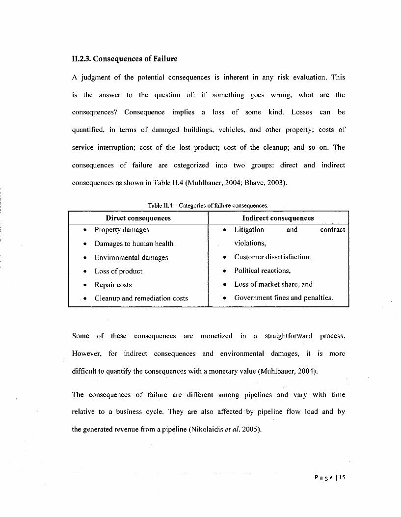
II.2.3. Consequences of Failure

A judgment of the potential consequences is inherent in any risk evaluation. This

is the answer to the question of: if something goes wrong, what are the

consequences? Consequence implies a loss of some kind. Losses can be

quantified, in terms of damaged buildings, vehicles, and other property; costs of

service interruption; cost of the lost product; cost of the cleanup; and so on. The

consequences of failure are categorized into two groups: direct and indirect

consequences as shown in Table II.4 (Muhlbauer, 2004; Bhave, 2003).

Table II.4 - Categories of failure consequences.

Direct consequences

• Property damages

• Damages to human health

• Environmental damages

• Loss of product

• Repair costs

• Cleanup and remediation costs

Indirect consequences

• Litigation and contract

violations,

• Customer dissatisfaction,

• Political reactions,

• Loss of market share, and

• Government fines and penalties.

Some of these consequences are monetized in a straightforward process.

However, for indirect consequences and environmental damages, it is more

difficult to quantify the consequences with a monetary value (Muhlbauer, 2004).

The consequences of failure are different among pipelines and vary with time

relative to a business cycle. They are also affected by pipeline flow load and by

the generated revenue from a pipeline (Nikolaidis et al. 2005).

P a g e | 15

Skipworth et al. (2001) made a comparison between the Whole Life Costing

(WLC) approach and the Risk Score-Based approach. Both approaches have the

same definition of risk as probability multiplied by consequences; however the

main difference between the two is how consequence is measured. In the WLC

approach, the consequence is to be defined in absolute values (in monetary

units) whereas in the Risk Score-Based approach, the consequence is defined by

a scoring system.

II.2.4. Water Main Failure Risk

This section provides an overview of the researches and various efforts related to water

main failure risk. In their efforts to assess the risk or the probability of pipeline failure,

researchers have used a broad variety of techniques. Some of the techniques are: fuzzy

logic (Marshall et al. 2005; Kleiner et al. 2006; Rajani et al. 2006), hierarchical

holographic modeling (Ezell et al. 2000), first order reliability modeling using Monte

Carlo Simulation (Sadiq et al. 2004), the analytical hierarchy process (Bandyopadhyay et

al. 1997; Al Barqawi, 2006), statistical non-homogeneous Poisson modes (Moglia et al.

2006; Rogers, 2006), fault tree analysis (Yuhua and Datao, 2005), probability density

function (Souza and Chagas, 2001), artificial neural networks (Christodoulou et al. 2003;

Al Barqawi, 2006), the non-homogenous Markov process (Kleiner et al. 2004), multi-

criteria decision making (Yan and Vairavamoorthy, 2003), and the Bayesian belief

network expert system (Hahn et al. 2002). These efforts are thoroughly explained in the

following paragraphs.

P a g e | 16

Marshall et al. (2005) evaluated the risk of failure of large diameter pre-stressed

concrete cylinder pipelines. A simplified strength model was developed to

evaluate the remaining strength of pre-stressed concrete pipe as it ages. This

model is derived from a process of inspecting pipelines using direct observations

and non-destructive tests. Many parameters are included in the fuzzy risk model,

such as: parameters affecting the rate of deterioration, parameters affecting

repair time, and the consequences of failure.

Kleiner et al. (2006) developed a methodology to evaluate pipeline failure risk

using the fuzzy logic technique. The model consists of three parts: possibility of

failure, consequence of failure and a combination of these two to obtain failure

risk. In the possibility of failure part, a seven-grade fuzzy set is used to describe

the asset condition rating and a nine-grade possibility of failure is used to reflect

the possibility of failure. The failure condition rating is fuzzified (remapped) on

the nine-grade possibility of failure. In the consequences of failure part, the

severity of an asset failure consequence is described in a nine-severity grade.

The consequences of failure can be in the form of direct cost, indirect cost, and

social cost. The risk of failure is assessed by combining the probability of failure

with the consequences of failure in nine fuzzy triangular subsets.

Rajani et al. (2006) used a fuzzy synthetic evaluation technique to translate

observations from visual inspection and non-destructive tests into water main

condition ratings. The process involves three steps, (1) fuzzijication of raw data

(measurements of the distress indicators), (2) aggregation of distress indicators

P a g e | 17

towards the condition rating, and (3) defuzzification that adjusts the condition

rating to a practical crisp format.

Ezell et al. (2000) introduced the Probabilistic Infrastructure Risk Analysis

model (IRAM). This system is developed for small community water supply and

treatment systems. It consists of four phases. In phase 1, the infrastructure

failure threats are identified by means of system decomposing. The target of

phase 2 is to provide information that describes the state of consequences for a

scenario executed against the system under study. An event tree is used together

with expert opinion to determine the failure probability of each path in the tree

and the inherent consequence. In phase 3, the consequence and the probability

of failure are combined together to identify the high risk factors, which are used

to manage the infrastructure in phase 4 by setting the acceptance risk level.

Sadiq et al. (2004) developed a method for evaluating the time-dependent

reliability of underground grey cast iron water mains, and for identifying the

major factors that contribute to water main failures. The first-order reliability

method is used, which employs a Monte Carlo simulation. In a Monte Carlo

simulation, a set of random values is generated for each input parameter of the

model (assumed to be independent), in accordance with a predefined probability

density function. However, the consequence of failure, which is a part of risk

calculation, is ignored and here the term "risk" refers solely to the probability of

failure. A sensitivity analysis showed that two of the parameters of the corrosion

model (the scaling constant for pitting depth and the corrosion rate inhibition

P a g e | 18

factor) were the largest contributors to the variability in the pipe's time to

failure.

Bandyopadhyay et al. (1997) established a cost-effective maintenance program

for a petroleum pipeline through risk analysis. The Analytical Hierarchy Process

(AHP) is used to carry out the risk assessment. The methodology followed in

this study starts with risk factors identification which can be listed as: corrosion,

external interference, acts of god, construction and materials defects, and other

reasons such as human error, operational error and equipment malfunction. The

second step is to formulate the risk structure model using AHP, which

determines the relative severity and probability of each risk factor. Then,

maintenance/inspection strategy requirements are determined in order to

mitigate the risk. Cost of failure is classified into four categories according to

the intensity and is estimated using the Monte Carlo simulation. A cost/benefit

analysis is carried out at the end to justify an investment proposal.

Moglia et al. (2006) explained the uses of the Decision Support System

PARMS-PLANNING which was developed to support the long term assessment

of costs and the implications of different management and operational asset

management strategies. Risks associated with different scenarios are assessed

using a standard risk management approach where risk is calculated by

combining the output of failure prediction models with the output of cost

assessment models. The failure prediction models use both a statistical Non-

Homogeneous Poisson model and a physical/probabilistic model that provide

failure rates and failure probabilities for each year into the future. The cost

P a g e | 19

model is based on user input. The specific costs are classified into: pipeline

renewal, valve insertions, pipe repairs, supply interruptions, and failure

consequences. In the risk calculation model, a risk-based approach is based on

the calculation of risk for different actions and scenarios where risk refers to an

uncertain event with unwanted consequences. This risk is calculated as the

statistical expectation of future costs caused by failure.

Yuhua and Datao (2005) analyzed the failure risk of oil and gas pipelines using fault tree

analysis. They divided the causes of failure of gas and oil pipelines into 44 failure causes,

which are categorized using fault tree analysis (FTA). The steps to be followed using

FTA are: 1) Select experts to form evaluation committee, 2) Convert linguistic terms to

fuzzy numbers, 3) Convert fuzzy numbers into fuzzy possibilities, and 4) Transform

fuzzy possibility scores into fuzzy failure probability (FFP). This method uses expert

opinion to evaluate the possibility of each event causing a failure. Next, the possibility of

failure is converted into a fuzzy possibility score and then into the fuzzy possibility of

failure. It is worth to note that the methodology explained above calculates the possibility

of failure for oil and gas pipelines due to each failure-causing event and does not consider

the actual condition of the pipeline in service.

Souza and Chagas (2001) applied the probability theory to evaluate and quantify

the risk associated with water pollution. This involves identifying risk sources,

failure probability, and the consequences of failure. The probability theory is

useful for a system with a consistent set of data. However, for systems without a

consistent set of data, the possibility of good results will be limited, because the

probability density function for all the sets of random variables is required in

P a g e | 20

this probability theory in order to measure the risk of any environmental system.

Fuzzy Set Theory could be a better means to determine this sort of risk when

only inconsistent data sets are available.

Christodoulou et al. (2003) used Artificial Neural Networks (ANN) to analyze

the preliminary water main failure risk in an urban area with historical break

data spanning two decades. The type of ANN used in this study is the

backpropagation algorithm. The outputs of backpropagation ANN are the age to

failure of each pipe segment, the observation outcome (a break or a non-break),

and the relevant weights of the risk factors. Their study indicates that the

number of previous breaks, the material, diameter, and length of pipe segments

are the most important risk factors for water main failures.

Al Barqawi (2006) designed two condition rating models for water mains using artificial

neural networks (ANN) and the analytical hierarchy process (AHP). In his research, he

considered only the deterioration factors (physical, operational, and environmental).

Using the ANN model, he concluded that the most important factors are breakage rate

and pipe age. However, when using an integrated ANN/AHP model, pipe age, pipe

material, and breakage rate are the most effective factors in evaluating the current

condition of water mains. He proposed a condition rating scale from 0 to 10 divided into

6 regions which describe the status of the water main.

Kleiner et al. (2004) used a fuzzy rule-based, non-homogeneous Markov process

to model the deterioration process of buried pipes. The deterioration rate at a

specific time is estimated based on the asset's age and condition state using a

P a g e 121

fuzzy rule-based algorithm. Then, the possibility of failure is estimated for any

age of the pipeline based on the deterioration model. The possibility of failure is

coupled with the failure consequence through a matrix approach to obtain the

failure risk as a function of the pipe's age.

Rogers (2006) developed a model to assess water main failure risk. He used the

Power Law form of a Non-Homogeneous Poisson Process (NHPP) and Multi-

Criteria Decision Analysis (MCDA) based on the Weighted Average Method

(WAM) to calculate the probability of failure. Moreover, the developed model

considers the consequence of failure using "what-if infrastructure investment

scenarios. The probability of failure and the consequences are directly related by

a multiplication operation in order to determine the associated risk.

Yan and Vairavamoorthy (2003) proposed a methodology to assess pipeline

condition using Multi-Criteria Decision Making (MCDM) techniques which

combine the available pipe condition indicators into one single indicator. Both

fuzzy set theory and its arithmetic corollaries are incorporated in the Composite

Programming to form Fuzzy Composite Programming (FCP). The model starts

by converting the linguistic variables into fuzzy numbers. These factors are

normalized to allow them to be combined and aggregated after assigning

weights to the different indicators. The output of the model is a fuzzy number

that reflects the condition of each pipeline, which is ranked accordingly.

Hahn (2002) developed a knowledge-based expert system to predict the criticality of

sewer pipelines. The expert system considers information about the environment and the

P a g e | 22

state of a sewer line through an extensive set of relationships that describe failure impact

mechanisms. The author used a Bayesian belief network to develop the expert system

denoted as SCRAPS "Sewer Cataloging, Retrieval and Prioritization System". Six failure

mechanisms that contribute to the likelihood of failure, and two consequences

mechanisms that contribute to the consequences of failure are included in the model. The

developed model was evaluated through three approaches: the consequence of failure, the

likelihood of failure, and both the consequence and the likelihood of failure. The output

of the model is the pipe line criticality or risk of failure and is categorized into three

ranges and groups (high, moderate, and low).

There are other research efforts that were undertaken in disciplines other than

water/sewer main pipelines such as reactor pipelines (Vinod et al. 2003),

petroleum pipelines (Bandyopadhyay et al. 1997; Yuhua and Datao, 2005), and

pipes transferring hydrogen sulfide (Santosh et al. 2006). These efforts are

explained in the following paragraphs.

Vinod et al. (2003) developed a study aiming at finding the realistic failure

frequency of pipe segments based on the degradation mechanisms to be

employed in Risk Informed In-Service Inspection in Pressurized Heavy Water

Reactor (PHWR) pipes. The primary PHWR piping is made of carbon steel

operating at around 300 °C. The model starts with erosion-corrosion rate

calculation and then applies this rate to the First Order Reliability Method to

determine the piping failure probability. After that, a Markov model is

developed to estimate the realistic failure probability, incorporating the effects

P a g e | 23

of In-Service Inspection which yields the failure probability to be used in Risk-

Informed In-Service Inspection.

Santosh et al. (2006) performed a study to utilize failure probability in a risk-

based inspection of pipelines transferring hydrogen sulphide. This involves

categorizing these pipelines based on their orders of failure probabilities. Two

steps are followed in this study: 1) estimation of the remaining strength of a

pipeline, and 2) evaluating the limit state function of a pipeline that defines the

failure criteria

II.3. Risk Evaluation Process and Modeling Approaches

II.3.1. Risk Process

There are five steps in a risk process: 1) Risk modeling, 2) Data collection and

preparation, 3) Segmentation, 4) Assessing risks, and 5) Managing risks

(Muhlbauer, 2004).

1) Risk modeling: a pipeline risk assessment model is a set of algorithms

or rules that use available information and data relationships to

measure levels of risk along a pipeline.

2) Data collection and preparation: the collection of all the required

information about the pipeline, including inspection data, original

construction information, environmental conditions, operating and

maintenance history, past failures, and so on. It results in data sets that

are ready to be used directly by the risk assessment model.

P a g e | 24

3) Segmentation: the process of dividing the pipeline into segments with

constant risk characteristics, or into measurable pieces. This is required

because the risk is rarely constant along a pipeline's length.

4) Assessing risks: the available risk model is applied to the data set in

order to evaluate the risk associated with each pipeline segment.

5) Managing risks: this step comprises the decision support process and

provides the tools needed to best optimize the allocation of resources.

It is worth mentioning that sometimes risk modeling and data collection is done

in the reverse order of this process (Muhlbauer, 2004).

H.3.2. Risk modeling

There are two types of risk assessment approaches ~ either quantitative or

qualitative. In a quantitative approach, the quantification of the probability and

severity of a particular hazardous event can be assessed and the risk is calculated

as the product: risk = probability x severity. The quantitative risk assessment

approach includes many methods such as Bayesian inference, fault tree analysis,

Monte Carlo analysis, and fuzzy arithmetic as a semi-quantitative method. In a

qualitative approach, the probability of an event may not be known, or not

agreed upon, or even not recognized as hazardous. Qualitative risk assessment

includes many methods such as Preliminary Risk/Hazard analysis (PHA),

Failure Mode and Effects analysis (FMEA), Fuzzy Theory, etc. (Kirchhoff and

Doberstein, 2006; Lee M. , 2006).

Generally, there are three types of risk models. They are matrix, probabilistic,

and indexing models (Muhlbauer, 2004).

P a g e | 25

i. Matrix models

Matrix models are one of the simplest risk assessment structures. This model

ranks pipeline risks according to the likelihood and the potential consequences

of an event by a very simple scale or a numerical scale (low to high or 1 to 5).

Expert opinion or a more complicated application might be used in this approach

to rank risks associated with pipelines. A simple risk matrix example is shown in

Figure II.2 (Muhlbauer, 2004).

High

O

a CO 3 ST « C O O

Low

4

3

2

1

5

4

3

2

6

5

4

3

7

6

5

4

Highest Risk

Lowest K Risk Low <(] i Likelihood ' j/High

Figure II.2 - Simple risk matrix (Muhlbauer, 2004).

I'I. Probabilistic models

Probabilistic risk assessment (PRA), sometimes called Quantitative Risk

Assessment (QRS) or Numerical Risk Assessment (NRA), is the most complex

and rigorous risk model. It is a rigorous mathematical and statistical technique

that relies heavily on historical failure data and event-tree/fault-tree analysis.

Page [26

This technique is very data intensive. The result of the model is the absolute risk

assessments of all possible failure events (Muhlbauer, 2004).

ill. Indexing models

Indexing models and similar scoring models are the most popular risk

assessment techniques. In this technique, scores are assigned to important

conditions and activities on the pipeline system that contribute to the risk, and

weightings are assigned to each risk variable. The relative weight reflects the

importance of the item in the risk assessment and is based on statistics where

available or on engineering judgment (Muhlbauer, 2004).

II.4. Fuzzy Logic

II.4.1. Introduction to Fuzzy Logic

Lotfi Zadeh developed fuzzy logic in the mid-1960s to solve the problem of representing

approximate knowledge that cannot be represented by conventional, crisp methods. A

fuzzy set is represented by a membership function. Any "element" value in the universe

of enclosure of the fuzzy set will have a grade of membership which gives the degree to

which the particular element belongs to the set (Karray and de Silva, 2004). Fuzzy theory

relies on four main concepts: (I) fuzzy sets: sets with non-crisp, overlapping boundaries;

(2) linguistic variables: variables whose values are both qualitatively and quantitatively

described with fuzzy sets; (3) possibility distributions: constraints on the value of a

linguistic variable imposed by assigning it a fuzzy set; and (4) fuzzy if-then rules: a

knowledge representation scheme for describing a functional mapping or a logic formula

P a g e | 27

that generalizes two-valued logic (Del Campo, 2004). More information is included in

"Appendix A: Introduction to Fuzzy Expert System".

II.4.2. Fuzzy Logic Application

Fuzzy logic has been used in many areas in water resources. Bogardi and

Duckstein (2002) listed some of them as follows:

• Fuzzy Regression: used where a casual relationship exits with few data

points.

• Hydrologic forecasting: Kalman filtering and fuzzy logic are used for

short-term and medium term forecasting.

• Hydrologic modeling: where traditional rainfall runoff models can be

replaced by fuzzy-rule systems with similar performance.

• Fuzzy-set geostatistics: can be used where imprecise and indirect

measurements and small data sets are combined in spatial statistical

analysis.

• Incorporation of spatial variability into groundwater flow and transport

modeling with fuzzy logic.

• Regional water resources management: when selecting among many

alternative management schemes under small data sets and with

imprecisely known or modeled objectives.

P a g e | 28

• Multi-criterion decision-making under uncertainty: can be used when

there are multiple and conflicting criteria and when the criteria

corresponding to alternative systems are imprecisely known.

• Fuzzy rule-based modeling: used in the classification of spatial

hydrometeorological events, climate modeling of flooding, modeling of

groundwater flow and transport, forecasting pollutants' transport in

surface water.

• Reservoir operation planning: applies fuzzy logic to derive operation

rules.

• Fuzzy risk analysis: used in evaluating uncertainty in any or all elements

of risk analysis (load, capacity, and consequence).

Fuzzy-based methods have been increasingly applied to civil and environmental

engineering problems in recent years, especially when the available information

(measured data or expert opinion) is vague and too imprecise to justify the use

of numbers. As a solution, fuzzy logic provides a language with syntax and

semantics to translate qualitative knowledge into numerical reasoning. Fuzzy

systems are used where crisp probabilistic models do not exist (Najjaran et ah

2004).

II.4.3. Fuzzy Expert Systems

i. Definition

Usually, systems that can process knowledge are called knowledge-based systems. One

of the most popular and successful knowledge-based systems is the expert system (Jin,

P a g e | 29

2003). Fuzzy logic can be used as a tool to deal with imprecision and the qualitative

aspects that are associated with problem solving and in the development of expert

systems. Fuzzy expert systems use the knowledge of humans, which is qualitative and

inexact. In many cases, decisions are to be taken even if the experts may be only partially

knowledgeable about the problem domain, or data may not be fully available. The

reasons behind using fuzzy logic in expert systems may be summarized as follows

(Karray and de Silva, 2004):

• The knowledge base of expert systems summarizes the human experts'

knowledge and experience.

• Fuzzy descriptors (e.g., large, small, fast, poor, fine) are commonly used in the

communication of experts' knowledge, which is often inexact and qualitative.

• Problem description by the user may not be exact.

• Reasonable decisions must be taken even if the experts' knowledge base may not

be complete.

• Educated guesses need to be made in certain situations.

ii. Fuzzy Expert System Application

An expert system consists of a knowledge base in the form of rules representing specific

domains of knowledge, plus a database (Jin, 2003). In this section, the use of expert

systems in the field of water resources is reviewed.

Nasiri et al. (2007) proposed a fuzzy multiple-attribute decision support expert system to

compute the water quality index and to provide an outline for the prioritization of

alternative plans.

P a g e | 30

Najjaran et al. (2004) developed a fuzzy logic expert system in order to establish a

criterion for predicting the deterioration of a cast/ductile iron water main using soil

properties. The fuzzy model determines the relationships between the output and inputs

of a system using antecedent and consequent propositions in a set of IF-THEN rules. The

input variables used in this model are selected from soil properties. The output is

corrosivity potential. The developed fuzzy model is imprecise for a certain range of

corrosivity potential either because the number of fuzzy rules in the rule base is

insufficient or the input and output partitions are not appropriately tuned in some range of

their universe of discourse.

ill'. Hierarchical fuzzy expert system

Acquiring knowledge for fuzzy rule-based systems can be achieved from human experts

or from experimental data using several methods (see A.8.2. Fuzzy Knowledge Rules

Acquisition). Mainly, there are three different approaches (Jin, 2003):

• Indirect Knowledge Acquisition

• Direct Knowledge Acquisition

• Automatic Knowledge Acquisition

Reducing the total number of rules and their corresponding computation requirements is

one of the most important issues in subjective fuzzy logic systems where the knowledge

base rules are solicited from experts in contract to the objective fuzzy systems where the

knowledge base rules are extracted from data. The "Curse of dimensionality" is an

attribute of subjective fuzzy systems since the number of rules and thus the complexity

increases exponentially with the number of variables involved in the model. To minimize

this problem, the hierarchical fuzzy system is proposed, where the overall system is

P a g e | 31

divided into a number of low-dimensional fuzzy systems. This has the advantage that the

total number of rules increases linearly with the number of the input variables. The

number of rules is greatly reduced by using a hierarchical fuzzy system (Lee et al. 2003).

There are several approaches to deal with hierarchical structures. One is that the output of

the last layer as a crisp value can be used as the input of the next layer in the hierarchical

fuzzy system. The advantage of this approach is that it will reduce the uncertainty of the

new result by reducing the number of fired rules in the new layer, but at the expense of

the information of uncertainty that is lost. Another approach is to consider the fuzzy

output of the last layer as the fuzzy input of the next layer. The advantage of this

approach is that it preserves the information about uncertainty. However, if the fuzzy set

is too wide, it will trigger too many rules in the new layer resulting in a very uncertain

result. Another approach is to decompose the defuzzification of the output that is used as

the input in the new layer into two or more crisp singletons (Gentile, 2004).

II.4.4. Expert Opinion Acquisition

Collecting information from experts will often require the use of qualitative

descriptive terms. Verbal labeling has some advantages, including ease of

explanation and familiarity. There are many emerging techniques of artificial

intelligence systems that aim at solving problems involving incomplete

knowledge and the use of descriptive terms through better use of human

reasoning. Fuzzy logic as an artificial intelligence system makes use of natural

language in risk modeling (Muhlbauer, 2004).

P a g e | 32

Expert opinions can be acquired with several methods; some of which are

(Cooke and Goossens, 2004):

1. Point Values: This method is used in the earlier expert systems like the

Delphi method where experts are asked to guess the values of unknown

quantities as a form of single point estimates. However, it has many

disadvantages which restrict the use of this method such as: scale

dependency, no indication of uncertainty in the assessments, and the

methodology of processing and combining the experts' judgment as

physical measurements.

2. Paired Comparisons: Experts are asked to rank alternatives pair-wise

according to certain criteria. Some of the disadvantages of this method

are: redundancy of the judgment data and no assessment of uncertainty.

3. Discrete Event Probabilities: Experts are asked to assess the probability of

occurrence of uncertain events as a point in the [0, 1] interval.

Disadvantages of this method are: careless formulations can easily

introduce confusion, and large finite populations are needed to adequately

measure the variable.

4. Distributions of Continuous Uncertain Quantities: Experts may be asked

to give a unique real value and to give a subjective probability

distribution. The probability distribution can be in the form of a

cumulative distribution function, density or mass function, or other

information such as the mean and standard deviation.

P a g e | 33

5. Conditionalisation and Dependence: Relevant variables must be specified

in the background information and the failure to specify background

information can lead experts to conditionalise their uncertainties in

different ways, which can introduce "noise" into the assessment process.

Variables whose values are not specified in the background information

can produce dependencies in the uncertainties of target variables. Experts

should be asked to address the dependencies in their subjective

distributions for these variables.

II.5. Risk and Condition Rating Scale

The risk of failure scale derives its importance from the need for a common language to

be spoken among the different authorities and municipalities. It is also used to compare

the condition and status of the infrastructure through a standardization process and to

allow decision makers to make informed decisions about the needs of an infrastructure to

be maintained or rehabilitated. Moreover, one of the important benefits of the failure risk

scale is to track the deterioration process of an asset over time. Developing a failure risk

scale usually depends on experts' opinions and experience or on the common practice

followed in managing the asset.

II.5.1. Different Types of Scales

Any risk scale consists mainly of three parts: numerical scale, linguistic scale, and

sometimes the associated corrective actions or maintenance plan. There are many types of

P a g e | 34

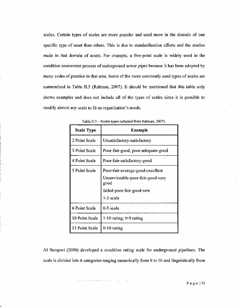
scales. Certain types of scales are more popular and used more in the domain of one

specific type of asset than others. This is due to standardization efforts and the studies

made in that domain of assets. For example, a five-point scale is widely used in the

condition assessment process of underground sewer pipes because it has been adopted by

many codes of practice in that area. Some of the more commonly used types of scales are

summarized in Table II.5 (Rahman, 2007). It should be mentioned that this table only

shows examples and does not include all of the types of scales since it is possible to

modify almost any scale to fit an organization's needs.

Table II.5 - Scales types (adapted from Rahman, 2007).

Scale Type

2 Point Scale

3 Point Scale

4 Point Scale

5 Point Scale

6 Point Scale

10 Point Scale

11 Point Scale

Example

Unsatisfactory-satisfactory

Poor-fair-good, poor-adequate-good

Poor-fair-satisfactory-good

Poor-fair-average-good-excellent

Unserviceable-poor-fair-good-very good

failed-poor-fair-good-new

1 -5 scale

0-5 scale

1-10 rating; 0-9 rating

0-10 rating

Al Barqawi (2006) developed a condition rating scale for underground pipelines. The

scale is divided into 6 categories ranging numerically form 0 to 10 and linguistically from

P a g e | 35

"critical to excellent" as shown in Figure II.3. He extracted this scale from experts'

opinions via a questionnaire.

0 3 4 6 8W 9 10 Very

Critic Poor Moderate Good Good Excellent

Figure II.3 - Underground pipelines condition rating scale.

Similar to Al Barqawi (2006), Rahman (2007) proposed a scale from 0 to 10 divided into

six condition grades (Figure II.4). The purpose of this scale is to fit the results of a

condition assessment of different elements of a drinking water treatment plant.

I R»3 i l l l f $ 3 0 3 4 6 8 „ 9 10

Very

Critic Poor Moderate Good Good Excellent

Figure 11.4 - Drinking water treatment plant condition rating scale.

Chughtai (2007) used a scale for sewer pipeline condition assessment which consists only

of integers and does not allow for intervals, as shown in Figure II.5. The reasoning

behind this is that the results of the condition assessment model are only integers and thus

there is no need for an interval scale.

P a g e | 36

D 1 • S D 1 v * 3 / v4 „ 5>

Y Y Light Medium Severe

Figure II.5 - Sewer pipeline condition assessment scale.

II.6. Summary

This chapter reviewed many topics that give an overview on how to approach the stated

problem. The topics included are: water main classification, risk of water main failure,

the risk evaluation process and modeling approaches, and fuzzy logic.

From the literature review, it is clear that the works that have addressed the problem of

water main failure risk have certain limitations, and therefore research that addresses the

problem with a broad, concrete, and robust approach is still needed. Certain researchers

have approached the problem in too shallow fashion, considering very few risk factors

which sometimes were limited to only the deterioration factors (condition rating) and/or

they did not consider the consequence of failure. Moreover, some of these researches

were so complicated in their derivation and usage that different municipalities and

authorities management teams are reluctant to use and depend on them. Other efforts

were too specific to certain conditions (such as pipe material, diameter, function, e tc . . )

and thus are not applicable to different water distribution networks. Some examples of

these researches were done by: Christodoulou et al. (2003), Yan and Vairavamoorthy

(2003), Kleiner et al. (2004), Sadiq et al. (2004), Kleiner et al. (2006), Rajani et al.

(2006) and Al Barqawi (2006). The most relevant and solid research was done by Rogers

(2006); however, there are some limitations inherent to his research such as: the model

P a g e | 37

uses the weighted average method which does not address the uncertainty and the model

is too sensitive to the weights of the factors. Moreover, Rogers' failure consequence

model is not well-established and depends solely on the input of the model user. In

addition, some of the risk factors are derived from a specific data set and seem to be more

reflective of that data set instead of reflecting the state of the art.

There are other research works that address the risk of failure of pipelines other than

water mains. Some of these researches cover areas such as: risk of failure of large

diameter pre-stressed concrete cylinder pipelines (Marshall et al. 2005), small community

water supply and treatment systems (Ezell et al. 2000), failure risk of sewers (Hahn,

2002), pressurized heavy-water reactor pipelines (Vinod et al. 2003), and pipelines

transferring hydrogen sulphide (Santosh et al. 2006). There have been more efforts to

address the risk associated with pipelines transferring petroleum materials (oil and gas)

due to the catastrophic consequence of their failure. Some of these studies are by

Bandyopadhyay et al. (1997), and Yuhua and Datao (2005).

Based on this exhaustive literature review, it is clear that there is a need to address the

problem of water main failure risk using a technique ~ such as fuzzy logic ~ that

considers the uncertainty usually associated with risk factors.

P a g e | 38

Chapter III: RESEARCH METHODOLOGY

The research methodology consists of eight stages as shown in Figure III. 1. It starts with

a comprehensive literature review of the risk of water main failure followed by data

collection, which in itself consists of two parts. A hierarchical fuzzy expert system

(HFES) is developed using model information data which is then underwent a

verification process. The next part of the research methodology is to develop a risk of

failure scale which will guide the network operators to best manage their networks. The

HFES model is used to assess the case study data collected from two municipalities. The

developed fuzzy expert application is based on MS ® Excel 2007 software.

III.l. Literature Review

All of the subjects related to the risk of water main failure are reviewed in order to have a

better overview of the topic, how others approached the problem, and how to best solve

the stated problem. In this research, the reviewed topics are water main classifications,

risk definition, different types of failure, different sources of risk associated with water

main failure, and consequences of failure. Different approaches in evaluation and

modeling the risk of failure such as matrix models, probabilistic models, and indexing

models are reviewed.

P a g e | 39

Literature Review

Study Risk Factors

Develop Hierarchical Fuzzy Expert Model

No

Yes

Risk of Failure Scale

Case Studies Applications

Excel-based Risk of Failure

Water main classification

Source of risk

Risk evaluation & modeling

Fuzzy logic

Types of scale

Environmental factors

Physical factors

Operational factors

Consequences factors

Model information

Case Study Data Sets

Data Collection

Figure III. 1 - Research methodology.

P a g e | 40

Some topics related to fuzzy logic are reviewed and can be listed as: literature review of

fuzzy logic and related research in the field of municipal networks, fuzzy logic process

and operation, and fuzzy expert systems. The use of experts' opinions in developing

fuzzy expert systems and hierarchy applications topics are reviewed as well. At last,

different scales used in the field of failure risk and condition assessment are reviewed.

III.2. Data Collection

The data collected for this research are used to develop the model and to apply the HFES

to case studies. The data needed to develop the model is collected from the literature and

by a questionnaire which is sent to experts in the field of water main infrastructure

management as shown in (Appendix B). Data for case studies are collected from two

municipalities that operate water mains. Three case studies data sets are introduced. The

first is the data set collected from the City of Moncton, New Brunswick. It contains data

for only seven out of the sixteen factors considered in this research; mainly the

quantitative factors. The second data set is constructed out of the first data set. Since the

first data set has some unavailable information about many risk factors (qualitative in

nature and do not require exact measurements or calculations), the second data set is

completed by randomly assuming the unavailable factors. The third data set is collected

from the City of London, Ontario. It contains data about nine failure risk factors.

Page 141

III.3. Hierarchical Fuzzy Expert System for Water Main Failure Risk

A hierarchical fuzzy expert system (HFES) is developed to estimate the risk of

water main failure. A Mamdani's fuzzy rules system is used as implication

operation in the fuzzy model. The hierarchical fuzzy model consists of four main

models which correspond to the four main factors: Environmental, Physical,

Operational, and Post-failure models. The results of these four models as crisp

values are used as crisp observations (input) to the fifth model which calculated

the risk of failure of water mains. Each of these branches has its own sub-factors

as shown in the hierarchy in Figure III.2.

In this research, in order to build the model knowledge base, the indirect

knowledge acquisition method (by means of a questionnaire and the available

literature) is used to gather the required information. However, a methodology is

proposed that is different from the traditional rules-building methodology, as

explained in detail in Section IV. 1.3. Expert knowledge base.

The first step in processing the data in the model is the fuzzification process.

This step uses the factors' membership functions to convert the real number into

a fuzzy number of a value in the period [0, 1]. In order to do this, each

membership function (linguistic variable) can be represented in an equation as

shown in Equation III. 1 (Del Campo, 2004), which converts the input number as

a real number (x) into a fuzzy number.

P a g e | 42

HA(x) = <

( ° (x~a) \b-a)

1 (C~X) Vc-J

^ 0

x < a a<x d

Equation IH.l

I Risk of Water main Failure i

Environmental Factors

Physical Factors

— Water Table Level [ —( Pipe Material

Daily Traffic

Operational Factors

Post Failure Factors

Pipe Diameter

Pipe Age

Protection Method

Hydraulic Factor j

Cost of Repair

Damage to Surroundings

/Business Disruption

Loss of Production

— Traffic Disruption

Type of Serviced Area

Figure III.2 — Hierarchical risk factors of water main failure.

P a g e | 43

After converting the real numbers of all the factors into fuzzy numbers, each of

the knowledge base rules is evaluated. The general form of the knowledge base

rules is as follows (Jin, 2003):

/?-': / / xx is AJt and x2 is AJ

2 and x3 is A3 and ...xn is AJn THEN y is Bj

Where Rj is the j-th rule, A{ (j = 1,2,... N,i = 1,2, ...n),B ; are the fuzzy

subsets of the inputs and outputs respectively.

This rule can be written mathematically as Equation III.2 (Jin, 2003):

r \ A A A * Equation III.2

VRi (X1,X2,X3, ..., xn, y) = nAj A pAj A A^/ - A / / , ; A MB

Where A denotes the minimum operator.

The consequent linguistic variable ff is to be chosen from a standard list of

seven linguistic variables (Extremely low, Very low, Moderately Low, Medium,

Moderately High, Very High, and Extremely High).

After evaluating each rule in the knowledge base, the membership value of each

consequent function (output linguistic variable) is aggregated using a maximum operation

as shown in Equation III.3 (Jin, 2003). In other words, the maximum membership value

of the ff consequent variable is used to truncate that consequent membership function for

later use in the defuzzification of the fuzzy output.

N

liR(x1,X2,X3,...,Xn,y) = \j[[iRj(x1,X2,X3,...,Xn,y)] Equation II1.3

/ = !

P a g e | 44

Where V denotes the maximum operation, R represents each of the consequent

membership functions as standardized to the list of (Extremely low, Very low,

Moderately Low, Medium, Moderately High, Very High, and Extremely High).

The next step is to defuzzify the consequent membership functions into one

crisp number. The defuzzification method used is the Center of Sum. It

calculates the center of gravity of each function individually and then average-

weights them by their areas. It has the advantage of being simple to program,

requiring minimal computer resources, and it gives reasonable results. The crisp

output of risk can be found using Equation III.4.

Crisp Risk Output =

extremely high . extremely high

y (Truncated Arean x Centeriodn) I y n=extremely low ' n=extreme

Truncated Areav

^extremely low I n=extremely low

Equation III.4

The procedure described above is generic and is applicable to every branch

(model) of the hierarchy (environmental, physical, operational, post-failure

factors branches (models), and risk of failure model which combines the four

models) to generate crisp output. Figure III.3 shows the data processing flow in

the physical risk model. The data processing flow of other factors' models are

identical to the physical factor model (only the sub-factors, their associated

membership functions (linguistic variables), and knowledge rules are different).

These crisp numbers are used as input to the risk of failure model and processed

as explained above. Figure III.4 shows the data processing in the Risk of Failure

P a g e | 45

model. It starts with the risk input from the four main models (branches of the

hierarchy) and then the model converts them into fuzzy numbers which then are

evaluated using the fuzzy knowledge base rules. The triggered fuzzy rules are

aggregated and defuzzified into a crisp number which represents the Risk of

Failure of the water main.

Physical risk factors

Fuzzy input variables

Fuzzy rules evaluation

Fuzzy output

Aggregation

Defiizzifi cation

Pipe diameter

Pipe Material

Pipe age

I

X 7

Protection Method

IF pipe diameter is a AND pipe material is b AND pipe age is c AND protection method is d THEN physical risk is e.

Crisp input to the next level of the hierarchy (Risk of failure model)

Figure III .3 - Physical risk model structure.

P a g e | 46

Failure risk factors

Physical

Fuzzy input variables

Fuzzy output

aggregation

Environmental Operational Post failure

I "

1= "•

I

A A A A A

/VVVIV5

— b . . _ M p . ' «

E = - | | :

""""! "

1 i It A A A A A . ' — "

AAAAA* ~~- ^ fVVVVH : i - ; •

1 A A A A A

AAAAA

— . ~ v »

LL_

—

Fuzzy rules Evaluation

r

>-

\ \ / X IF Physical risk is a AND Environmental risk is b AND Operational risk is c AND Post failure risk is of THEN Risk of Failure is e.

i '

-\

J

Defiizzification Crisp Output

Figure I1I.4 - Risk of failure model structure.

III.4. Model Analysis and Verification

A sensitivity analysis is carried out in order to test the sensitivity of the model

and its stability, and to insure that it is performing as expected. The sensitivity

analysis is done by assuming many scenarios; testing most weighted factors,

testing, the effect of weights on the model, testing the model performance from

the least risky to highest risky status of the factors, etc.... Model verification is

carried out by using a validated model to compare the results of the proposed

model with the validated model. The model used for verification is the AHP

deterioration model developed by Al Barqawi (2006) which can only evaluate

the deterioration part of the proposed model.

P a g e 147

111.5. Risk of Failure Scale

In light of the reviewed literature, a risk of failure scale is proposed to help decision

makers in water resources management companies/municipalities make an informed

decision. The scale ranges numerically from 0 to 10, where 10 indicates the most risky

condition of the pipeline and 0 indicates the least risky condition. Linguistically, the scale

is divided into five groups or regions which describe the risk of pipeline failure and the

required corrective actions to be taken if needed, as explained later in Section "V.8.

Proposed Risk of Failure Scale". The number of proposed groups and their ranges and

associated corrective actions are likely to be changed to best suit municipality's strategies

and risk tolerance.

111.6. Case Studies Application

Three case studies data sets are collected and used to show the application of the

developed model. The case studies results are studied and analyzed and some

recommendations are proposed depending on the results of the model. In case study one,

the results show that the condition of the network is fair (66% of the network) with some

parts of the network requiring mitigation action in the short-term plan. However, the

results of case study two show that the condition of the network is risky (50%) to fair

(47%) with some parts of the network requiring immediate mitigation action. In case

study three, the condition of the network is fair (50%) to risky (45%) with some parts of

the network require immediate mitigation action.

P a g e | 48

111.7. Excel-Based Application Development

An application is built to implement the developed model. The application is

based on MS© Excel 2007. The application consists of many spreadsheet files.

It is controlled through an Excel file called "Navigation". This file contains all

the step by step instructions that will guide the user to the easy use of the

application. Other spreadsheet files represent the four branches of the hierarchy,

the risk of failure model, etc... A full review of the application is explained in

"Chapter VI: Excel-Based Application Development".

111.8. Summary

This chapter presented the research methodology followed in this thesis. This

methodology includes the literature review of the risk of water main failure, data

collection (which consists of model information data and case studies data) HFES model

development, the risk of failure scale, case studies evaluation, and the development of an

Excel-based application.

P a g e | 49

Chapter IV: DATA COLLECTION

The data collection consists of two stages which are required to develop and run the fuzzy

expert system. In stage one, the information needed to build the model is collected. In

stage two, real network characteristics are gathered and analyzed by the developed

model. The process of data collection and its parts is shown in Figure IV. 1.

Factors' weights Factors' performance impact

Water mains attributes

Collected by:

- Questionnaire

Collected by:

- Literature review

-Questionnaire

'Collected from:

• Municipalities

Figure IV. 1 - Water main data collection process.

P a g e | 50

IV.l. Model Information

The information needed to develop the model consists of two parts: factors' weights and

factors' performance impact. The majority of information is gathered from the literature.

The information that can not be collected from the literature is collected via a

questionnaire. A sample questionnaire is shown in Appendix B. The two parts of the

model information are as follows:

IV.1.1. Weights of Factors

In this section, the relative weight of each factor at each level of the hierarchy is

collected. This could be the answer to the question of "What is the strength of the factor

in contributing to the failure event?" This information is collected by a questionnaire. The

questionnaire was sent to fifty-eight experts (designers, operators, consultants,

researchers), and feedback was received from only twenty, giving an average response of

34% as shown in Figure 1V.2.

Figure IV.2 - Questionnaire statistics.

P a g e |51

Geographically, the received responses can be summarized according to their locations as

follows: Quebec 4 responses, Alberta 6, Ontario 6, British Colombia 2, New Brunswick

1, and Saskatchewan 1 response. Figure IV.3 shows the percentages of received

responses from each participating province.

H

- • » & * • : + . - . ; • . • • . « * • ' * •

• • • • • '?*: ft: ; V j j

New brunswick 5%

atchew|$ 5%

Figure IV.3 - Percentages of received questionnaires from each Canadian province.

Table IV.1 shows the collected factors' weights. The local weight of each risk sub-factor

shown in that column is comparable only to its group of risk factor (hierarchy branch).

The weights of the sub-factors can be compared to those in other groups by multiplying

the sub-factors' local weights by the main factor weight of where they belong, as shown

in the Global Weights column. It is worth mentioning that the developed model can use

either the local or global weights since each main risk factor is treated and modeled

separately. It is obvious that pipe age has the highest weight and thus it has the most

effect on the model. Figure IV.4 shows a graph of the normalized global weights of the

P a g e | 52

failure risk factors. From this graph, it can be deduced that pipe age has the highest effect

among the other factors, followed by pipe material and breakage rate. By reviewing the

values of standard deviation, the highest value is 20, the lowest is 4, and the average is

10, which are acceptable values.

Table IV. 1 -Risk of failure factors' weights.

Main Risk Factor


Physical Factors

Operational Factors

Post-Failure Factors

Factor Weight

19

43

28

20

Risk sub-factor

Soil Type Average Daily Traffic

Water Table Level

Pipe Material

Pipe Diameter

Pipe Age

Protection Method

Breakage Rate Hydraulic Factor Water Quality Leakage

Cost of Repair

Damage to surroundings

Loss of Production

Traffic Disruption


Sub-factors local

weights 42

13

20

30

19

40

15

35 13

17

20

20

21

18

17

14

Stand ard

devia tion

9.2

5.0

6.8

12.1 9.1

16.1

8.2

10.8 6.6 4.4

5.9

7.1

5.7

6.0

5.3

5.6

Global weights

798

247

380

1290

817

1720

645

980 364 504 560

400

420

360

340

280

Normalized Global weights

46

14

22

75

48

100

38

57 21

29 32

23

24

21

20

16

P a g e | 53

100 -

90 -

80 -

70 -

oU -

50 -

40 -

30 -

20 -

10 -

0

.inq

.46. __™.

1 H 22

III "o

i i * 1

Pip

e M

a

Pip

e D

iar

Pip

ectio

n M

e

1

5 Z _ _ _ _ _

• - • I " a 32

I ' l l QJ 1- > QJ

Mil B

reak

age

ydra

ulic

F

Wat

er Q

.

Le«

X

23 J l 21 20 nil mill fin i m mil

.«- IA c c n>

epa

ding

ctio

ptio

Are

Cos

t of R

o su

rrou

n

5 of P

rodu

affic

Dis

ru

f Ser

vice

d

Dam

age

t

Los Tr

Typ

eo

Figure IV.4 - Risk factors normalized global weights.

IV.1.2. Factors Performance Impact

In this section, performance assessment of the different factors considered in this project

(as shown in Figure III.2) is collected mainly from the literature. The information about

the factors where the performance is not clear or is missing is collected via a

questionnaire. The performance or behavior of 13 out of 16 factors are collected from the

literature review: soil type, daily traffic, pipe diameter, pipe material, pipe age, protection

method, breakage rate, hydraulic factor, water quality, leakage rate, cost of repair, traffic

disruption, and type of serviced area. The remaining required information is collected in

the form of a questionnaire sent to experts in order to gather their opinion and experience

P a g e | 54

about the behavior and characteristic of the water main network. The performance impact

of only three factors are collected via the questionnaire: water table level, damage to

surroundings/business disruption, and loss of production. This information is gathered in

the form of (if-then) or (cause-effect) where the answer is standardized to the following

list: "Extremely High, Very High, Moderately High, Medium, Moderately Low, Very Low,

Extremely Low"

The factors' performance impact is shown below:

/. Environmental Factors

The environmental factors are type of soil, water table level, and average daily traffic.

The performance of the type of soil and average daily traffic factors are collected from

the literature and are shown in Table IV.2 and Table 1V.4 respectively. Water table level

factor performance is collected by a questionnaire and shown in Table IV.3.

Table IV.2 - Type of soil factor performance.

Factor performance

if soil is Very lightly deteriorative

if soil is Lightly deteriorative

if soil is Moderately deteriorative

if soil is Highly deteriorative

if soil is Very highly deteriorative

Impact on risk

then the risk of failure is Extremely Low

then the risk of failure is Very Low

then the risk of failure is Medium

then the risk of failure is Very High

then the risk of failure is Extremely High

Table IV.3 - Water table level factor performance.

Factor performance

if WT is rarely present

ifWTis seasonally present

if WT is always present

Impact on risk



then the risk of failure is Moderately High

P a g e | 55

Table IV.4 - Daily traffic factor performance.

Factor performance

if ADT is Very light

ifADTis Light

if ADT is Moderate

ifADTis Heavy

if ADT is Very heavy

Impact on risk






I'I. Physical Factors

This category of factors includes pipe diameter, material, age, and pipe

protection method. The performance of the different factors are shown in Table

IV.5 through Table IV.8. These factors' performance is collected from the

literature.

Table IV.5 - Pipe diameter factor performance.

Factor performance

if dia. is small (< 250 mm)

ifdia. is medium (between 250 to 500)

Impact on risk



Table IV.6 - Pipe material factor performance.

Factor performance

ifADTis Concrete

ifADTis Asbestos

ifADTis PVC

ifADTis PE

ifADTis Ductile iron

ifADTis Steel

ifADTis Cast iron

if ADT is Cast iron post war

Impact on risk









P a g e | 56

Table IV.7 - Pipe age factor performance.

Factor performance

if age is new (0 yrs < Age < 10 yrs)

if age is young (10 yrs < Age < 30 yrs)

if age is medium (30 < Age < 50)

if age is old (50 yrs < Age < 70 yrs)

if age is very old (> 70 yrs)

Impact on risk






Table IV.8 - Protection methods factor performance.

Factor performance

if pipe has Cathodic protection

if pipe has Lining/Coating

if pipe has none

Impact on risk




HI. Operational Factors

Operational factors include breakage rate, hydraulic factor (hazen-william coefficient),

water quality, and leakage rate. The factors' performance is collected from the literature

and are shown in Table IV.9 through Table IV. 12.

Table IV.9 - Breakage rate factor performance.

Factor performance

if breakage rate is low (< 0.5 brk/km/yr)

if breakage rate is average (bet 0.5 and 3)

if breakage rate is high (> 3 brk/km/yr)

Impact on risk




P a g e | 57

Table IV. 10 - Hydraulic factor performance.

Factor performance

if pipe is very rough (C-factor < 40)

if pipe is rough (60 > C-factor > 40)

if pipe is medium (80 > C-factor > 60)

if pipe is smooth (100 > C-factor > 80)

if pipe is very smooth (C > 100)

Impact on risk






Table IV. 11 - Water quality factor performance.

Factor performance

if WQ is very good

if WQ is good

ifWQis acceptable

ifWQis bad

if WQ is very bad

Impact on risk






Table IV. 12 - Leakage rate factor performance.

Factor performance

if leakage is very low

if leakage is low

if leakage is medium

if leakage is high

if leakage is very high

Impact on risk






iV. Post failure Factors

This category of factors represents the consequence of failure. It includes five

factors. The performance of cost of repair, traffic disruption, and type of

serviced area and are shown in Table IV. 13, Table IV. 16, and Table IV. 17 are

collected from literature. Damage to surrounding and loss of productions

P a g e | 58

factors' performance is collected by a questionnaire as shown in Table IV. 14

and Table IV. 15.

Table IV. 13 - Cost of repair factor performance.

Factor performance

if repair cost is very low

if repair cost is low

if repair cost is medium

if repair cost is high

if repair cost is very high

Impact on risk






Table IV. 14 - Damage to surroundings factor performance.

Factor performance

if failure in Industrial area

if failure in Commercial area

if failure in Residential are

Impact on risk




Table IV.15 - Loss of production factor performance.

Factor performance

if pipe is small & redundant

if pipe is medium & redundant

if pipe is small & not redundant

if pipe is medium & not redundant

Impact on risk


then the risk of failure is Moderately Low



Table IV. 16 - Traffic disruption factor performance.

Factor performance

if failure is Very lightly disruptive

if failure is Lightly disruptive

if failure is Moderately disruptive

if failure is Highly disruptive

if failure is Very highly disruptive

Impact on risk

then the cost of failure is Extremely Low

then the cost of failure is Very Low

then the cost of failure is Medium

then the cost of failure is Very High

then the cost of failure is Extremely High

P a g e | 59

Table IV. 17 - Type of serviced area factor performance.

Factor performance

if failure stops service to Industrial area

if failure stops service to Commercial area

if failure stops service to Residential are

Impact on risk

then the cost of failure is Very High

then the cost of failure is Medium

then the cost of failure is Moderately Low

v. Risk of failure Factors

This contains the four main risk of failure factors as shown in Figure III.2. It

includes environmental, physical, operational and post failure factors. There

performance is shown in Table IV. 18 to Table IV.21.

Table IV. 18 - Environmental factor performance.

Factor performance

if environmental risk is Extremely Low

if environmental risk is Very Low

if environmental risk is Moderately Low

if environmental risk is Medium

if environmental risk is Moderately High

if environmental risk is Very High

if environmental risk is Extremely High

Impact on risk








Table IV. 19 - Physical factor performance.

Factor performance

if physical risk is Extremely Low

if physical risk is Very Low

if physical risk is Moderately Low

if physical risk is Medium

if physical risk is Moderately High

if physical risk is Very High

if physical risk is Extremely High

Impact on risk








P a g e | 60

Table IV.20 - Operational factor performance.

Factor performance

ifoperationalriskis Extremely Low

ifoperationalriskis Very Low

if operational risk is Moderately Low

if operational risk is Medium

if operational risk is Moderately High

ifoperationalriskis Very High

if operational risk is Extremely High

Impact on risk








Table IV.21 - Post failure factor performance.

Factor performance

if post failure risk is Extremely Low

if post failure risk is Very Low

if post failure risk is Moderately Low

if post failure risk is Medium

if post failure risk is Moderately High

if post failure risk is Very High

if post failure risk is Extremely High

Impact on risk








IV.1.3. Expert knowledge base

The next step is to combine the collected factors' weights and factors

performance in a form that can be used in an expert system and represents the

knowledge of the experts. To do so, a rules building methodology will be used

which uses weighted average method to combine the factors' performance

depending on the weights. The reason behind using this methodology over the

traditional methodology of directly soliciting the rules from experts is that the

traditional methodology requires the expert to evaluate the performance of a

P a g e | 61

huge number of rules; this process is exhausting and time consuming and the

human expert will most probably not carry out this task. To overcome this major

drawback to using a traditional methodology in rules extraction, a new

methodology is proposed. The proposed new methodology will ask the expert to

evaluate the performance of each factor independent of other factors as collected

in IV.1.2. Factors Performance Impact (e.g. IF pipe age is old THEN the risk of

failure is High). Moreover, the expert is also asked to give a weight to each

factor which reflects the contribution of each factor to the risk of water main

failure as collected in IV. 1.1. Weights of Factors. The general outlines of the

proposed method are explained in Figure IV.5. The proposed method shares an

idea with the method originally developed by Shaheen (2005). The shared idea

is the use of the impact of each factor individually together with its weight

(importance) to generate the equivalent impact of the rules. The main difference

between the proposed method and the one developed by Shaheen (2005) is the

use of the average weighted method to choose the equivalent impact of the rule

instead of using a normalization process. Moreover, both the factors'

performance impact scale and equivalent ranges of impact scale are derived

from the performance of the model (fuzzy model to be built in the next chapter)

instead of using two different scales and using a normalization process. Using

the weights of factors, the combined performance impact of the different factors

is calculated using the weighted average method. The followings shows the

steps followed in finding the equivalent impact of different combinations of each

four branches of the hierarchy and the main level of the hierarchy.

P a g e | 62

Rulex: If Factorx is performance(x) and Factor2 is performance(v) and... and Factorn is performance(z)

then equivalent combined impact is XXX 1 In order to find the equivalent combined impact of each rule, it is calculated as follows (example of last

rule x.v.z): . _ W!XF1CX +W2XF2Cv+-+WnxFnCz

W1+W2+~+W„ Equivalent impact •

Where

F1CX = performance impact value of factor 1

F2CV = performance impact value of factor 2

FnCz = performance impact value of factor n

These values are

found using this scale

E 3 <D O

1X1

0.28

Low

c: >

1.67

tel

2 S 0) O

o

3.33

e a S 5

5

tel

2 "& •S 5? i )

6.67

s i £•

f 8.33

ely

a, .5? X

LU

9.72

After that, the equivalent impact value is matched against the ranges of the scale shown below

CD

E 5 CD O

"x LU

0 0.83

Low

V

er

|

2.5

rate

ly

w

-S -> o 5 |

4.17

E

^ l 5.83

(U

<u ~ T3 I

o 5 |

7.5

Hig

h

Ver

mel

y E

xtr

9.17

JZ

10

Figure IV.5 - Proposed methodology for fuzzy rules extraction.

P a g e | 63

i. Environmental Factors

1) Number of performance combination

The number of performance combination can be calculated for the

environmental factors by multiplying the number of performance stages

of the factors. In this research, the number of different performance

combinations needed to cover all the combination possibilities can be

found as:

number of environmental rules

= 5 (soil type)

X 5 (average daily traffic)

x 3 (water table level) = 75 rules

Equation IV. 1

Example: IF Type of soil is moderately deteriorative AND Average daily

traffic is extremely high AND Water table level is rarely present.

2) Weights of factors

This is discussed in section IV.1.1. Weights of Factors. The normalized

global weights or the local weights can be used in this process as shown

in Table IV.22.

Table IV.22 - Environmental factors weights.

Main Risk Factor


Risk sub-factor

Soil Type Average Daily Traffic Water Table Level

Sub-factors local

weights 42 13 20

Global weights

798 247


46 14

380 | 22

P a g e | 64

3) Factors performance impacts

The factors performance impacts at different stages (collected in section

IV. 1.2. Factors Performance Impact) is measured by a scale as shown in

Figure IV.6.

ely

E 5 S 3

Ext

0.28

S _ l

£r 0J

>

1.67

>• Ol

2 5 •

tel

ra .c 0) .2?

T3 X o

1 6.67

x: BO X

2->

8.33

ely

E -5, S f

Ext

9.72

Figure IV.6 - Factor performance impact scale

To illustrate how this scale works, an example is given below:

• If soil type is moderately deteriorative then risk of failure is medium (5

impact value)

• If average daily traffic is very heavy then risk of failure is extremely high

(9.72 impact value)

• If water table level is rarely present then the risk of failure is extremely

low (0.28 impact value)

4) Factors performance combined impact

In order to find the combined impact of the different factors' performance,

weighted average method is used as shown in Equation IV.2.

Equivalent impact = Y.(i™.pcLct x Weight) of each factor

£ factors Weights Equation IV.2

P a g e | 65

This equivalent impact is matched against another scale that is divided

into ranges of different equivalent impact as shown in Figure IV.7.

>-Ol

OJ O

s LU

0 0.83

Low

£• 01

>

2.5 ra

tely

w

eu O

O

2

4.17

E .3

OJ

5

5.83

rate

ly

01 —

o 5

7.5

Hig

h

£• Ol

> S x « LLI

9.17 10

Figure IV.7 - Equivalent ranges of combined impact.

Both impact values scale and impact ranges scale are derived from the

shape of membership functions of the consequent of the fuzzy system to

be developed in next chapter. Continuing the example shown above, the

combined impact is found and the rule is established. So,

Equivalent impact Equation IV.3

(5 x 42) + (9.73 x 13) + (0.28 x 20) = = 4.56

(42 + 13 + 20)

Matching the value of equivalent impact against the scale in Figure IV.7

yields that the linguistic equivalent impact is medium. So the rule will be

completed as:

IF Type

extremely

of soil is moderately deteriorative

high AND Water table

failure is Medium.

level is

AND Average

rarely present

daily

THEN

traffic

risk

is

of

P a g e | 66

All other factors' performance impacts combinations (75 combinations)

can be found using this approach. The developed form of rule can be used

in an expert system such as fuzzy expert system. A sample of these rules

are shown in Table IV.23.

Table IV.23 - Sample environmental factors performance combined impact.

Rule No.

1

2

3

4

5

6

7

•

73

74

75

Factors' performance

Soil

Very highly deteriorative






Very highly deteriorative :

:

Very lightly deteriorative



Traffic

Very heavy

Very heavy

Very heavy

Heavy

Heavy

Heavy

Moderate

Very light

Very light

Very light

Water Table

always present

seasonally present

rarely present

always present

seasonally present

rarely present

always present

always present

seasonally present

rarely present

Combined Impact

linguistic

Very High

Extremely High

Moderately High

Very High

Extremely High

Moderately High

Very High

Very Low

Moderately Low

Extremely Low

ii. Physical Factors



physical factors by multiplying the number of performance stages of the

factors. In this research, the number of different performance


found as:

P a g e | 67

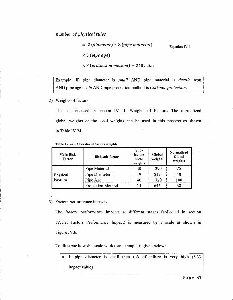
number of physical rules

= 2 (diameter) x 8 (pipe material)

x 5 (pipe age)

x 3 (protection method) = 240 rules

Equation IV.4

Example: IF pipe diameter is small AND pipe material is ductile

AND pie: it pipe diameter is smau /\INL> pipe material is aucin

pipe age is old AND pipe protection method is Cathodic protection.

iron


This is discussed in section IV. 1.1. Weights of Factors. The normalized


in Table 1V.24.

Table IV.24 - Operational factors weights.

Main Risk Factor

Physical Factors

Risk sub-factor

Pipe Material Pipe Diameter Pipe Age Protection Method

Sub-factors local

weights

Global weights

30 J 1290 19 817 40 15

1720 645


75 48 100 38




Figure 1V.6.


• If pipe diameter is small then risk of failure is very high (8.33

impact value)

_ _ _ _ _

• If pipe material is ductile iron then risk of failure is very low (1.67

impact value)

• If pipe age is old then the risk of failure is very high (8.33 impact

value)

• If pipe protection method is cathodic protection then the risk of

failure is very low (1.67 impact value)


In order to find the combined impact of the different factors'

performance, weighted average method is used as shown in Equation IV.2

which is matched against another scale that is divided into ranges of

different equivalent impact as shown in Figure IV.7.

Continuing the example shown above, the combined impact is found and

the rule is established. So,

Equivalent impact

_ (8.33 X 19) + (1.67 X 30) + (8.33 X 40) + (1.67 X 15) Equation IV.5

~ (19 + 30 + 40 + 15)

= 5.4



completed as:

P a g e | 69

IF pipe diameter is small AND pipe

is old AND pipe

failure is Medium.

protection method

material is ductile iron

is Cathodic protection

AND pipe

THEN risk

age

of





Table IV.25 — Sample physical factors performance combined impact.

Rule No.

1

2

3

4

5

6

7

8

9

:

238

239

240

pipe type

Concrete

Concrete

Concrete

Concrete

Concrete

Concrete

Concrete

Concrete

Concrete :

:

Cast iron post war

Cast iron post war

Cast iron post war


pipedia

Small

Small

Small

Small

Small

Small

Small

Small

Small :

medium

medium

medium

pipe age

Very old

Very old

Very old

old

old

old

medium

medium

medium

New

New

New

protection

Cathodic protection

Lining\Coating

none

Cathodic protection

Lining\Coating

none

Cathodic protection

Lining\Coating

none

:

Cathodic protection

Lining\Coating

none

Combined impact

linguistic

Moderately High

Moderately High

Moderately High

Moderately High

Moderately High

Moderately High

Medium

Medium

Medium

Moderately Low

Moderately Low

Moderately Low

Hi. Operational Factors



operational factors by multiplying the number of performance stages of

the factors. In this research, the number of different performance

P a g e | 70


found as:

number of operational rules

= 3 (breakage rate)

Equation IV.6 x 5 (hydraulic factor)

x 5 (water quality)

x 5 (leakage rate) — 375 rules

Example: IF breakage rate is high AND hydraulic factor (roughness test)

is rough AND water quality is very bad AND leakage rate is medium.




in Table IV.26.


Main Risk Factor

Operational Factors

Risk sub-factor


Sub-factors local

weights

35 13 17 20

Global weights

980 364 504 560


57 21 29 32




Figure IV.6.

P a g e | 71


• If breakage rate is high then risk of failure is extremely high (9.17

impact value)

• If hydraulic factor (roughness test) is rough then risk of failure is

very high (8.33 impact value)

• If water quality is very bad then the risk of failure is extremely

high (9.17 impact value)

• If leakage rate is medium then the risk of failure is medium (5

impact value)








Equivalent impact

_ (9.17 X 35) + (8.33 X 13) + (9.17 X 17) + (5 X 20) Equation IV.7 ~ (35 + 13 + 17 + 20)

= 8.06

P a g e | 72


yields that the linguistic equivalent impact is very high. So the rule will

be completed as:

IF breakage rate is high AND hydraulic factor (roughness test) is rough

AND water quality is very bad AND leakage rate is medium THEN risk

of failure is very high.





Table IV.27 - Sample operational factors performance combined impact.

Rule No.

1

2

3

4

5

6

7

8

9

:

;

373

374

375

breakage

low

low

low

low

low

low

low

low

low

:

high

high

high


roughness

very rough

very rough

very rough

very rough

very rough

very rough

very rough

very rough

very rough :

:

very smooth

very smooth

very smooth

W. Quality

Very good

Very good

Very good

Very good

Very good

Good

Good

Good

Good

:

Very bad

Very bad

Very bad

Leakage

very high

high

medium

low

very low

very high

high

medium

low

:

medium

low

very low

combined impact |

linguistic

Moderately Low

Moderately Low

Moderately Low

Very Low

Very Low

Medium

Moderately Low

Moderately Low

Very Low

:

Moderately High

Moderately High

Moderately High

P a g e | 73

iv. Post failure Factors


The number of performance combination can be calculated for the post

failure factors by multiplying the number of performance stages of the



found as:

number of post failure rules

= 5 (repair cost)

x 3 (damage to surrounding)

Equation IV. 8 x 4 (loss of production)

x 5 (traffic disruption)

x 3 (type of serviced area)

= 900 rules

Example: IF repair cost is low AND damage to surrounding is in

industrial area AND loss of production is in small redundant pipe AND

traffic disruption is lightly disruptive AND type of serviced area is

industrial.


This is discussed in section IV.1.1. Weights of Factors. The normalized


in Table IV.28.

P a g e | 74


Main Risk Factor


Risk sub-factor

Sub-factors local

weights

Cost of Repair 20

Global weights


400 1 23

Damage to surroundings 21 j 420 Loss of Production 18 360 Traffic Disruption 17 340

Type of Serviced Area j 14 | 280

24 21 20

16



IV.1.2. Factors Performance Impact) is measured by a scale as shown in

Figure IV.6.


• If repair cost is low then risk of failure is very low (1.67 impact

value)

• If damage to surrounding is in industrial area then risk of failure is

extremely high (9.72 impact value)

• If loss of production is in small redundant pipe then the risk of

failure is very low (1.67 impact value)

• If traffic disruption is lightly disruptive then the risk of failure is

very low (1.67 impact value)

• If type of serviced area is industrial then the risk of failure is very

high (8.33 impact value)

P a g e | 75








Equivalent impact

_ (1.67 x 20) + (9.72 x 21) + (1.67 x 18) + (1.67 x 17) + (8.33 + 14

_ (20 + 21 + 18 + 17 + 14) E q ]

= 4.58



completed as:

IF repair cost is low AND damage to surrounding is in industrial area

AND loss of production is in small redundant pipe AND traffic

disruption is lightly disruptive AND type of serviced area is industrial

THEN risk of failure is medium.





P a g e | 76

Table IV.29 - Sample post failure factors performance combined impact.

Rule No.

1

2

IT)

4

5

6

7

998

999

900

Factors' performance Combined impact

Repair Damage to , , „ , . Traffic Type of . . . . .. Loss of Production 1 . . „ . Linguistic

cost Surrounding Disruption Service area

very high

very high

very high

very high

very high

very high

very high

very low

very low

very low

Industrial

Industrial

Industrial

Industrial

Industrial

Industrial

Industrial

Residential

Residential

Residential

Small-Redundant

Small-Redundant

Small-Redundant

Small-Redundant

Small-Redundant

Small-Redundant

Small-Redundant

medium-not Redundant



Very heavy

Very heavy

Very heavy

Heavy

Heavy

Heavy

Moderate

Very light

Very light

Very light

Industrial

Commercial

Residential

Industrial

Commercial

Residential

Industrial

Industrial

Commercial

Residential

Very High

Moderately High

Moderately High

Very High

Moderately High

Moderately High

Moderately High

Moderately Low

Moderately Low

Very Low

v. Risk of failure Factors


The number of performance combination can be calculated for the main

risk factors by multiplying the number of performance stages of the



found as:

number of post failure rules

— 7 (environmantal factor)

x 7 (physical factor)

x 7 (operational factor)

x 7 (post failure factor) = 2401 rules

Equation IV. 10

P a g e | 77

Example: IF environmental factor is moderately low AND physical factor

is very high AND operational factor is moderately high AND post failure

factor is very low.




in Table IV.28.


Main Risk Factor

Main risk factors

Risk sub-factor

Environmental factor

Physical factor Operational factor

Post failure factor

Sub-factors local

weights

19

43

28 20

Normalized weights

44

100

65 46



IV.1.2. Factors Performance Impact) is measured by a scale as shown in

Figure IV.6.


•

•

If environmental factor is moderately

moderately low (3.33 impact value)

If physical factor

impact value)

is very high then risk

low then

of failure

risk of

is very

failure is

high (8.33

P a g e | 78

• If operational factor is moderately

moderately high (6.67 impact value)

• If post failure factor

(1.67 impact value)

high then the risk

is very low then the risk of failure

of

is

failure is

very low



performance, weighted average method is used as shown in Equation 1V.2





Equivalent impact

_ (3.33 x 19) -r (9.72 x 43) + (6.67 x 28) + (1.67 x 20) - (19 + 43 + 28 + 20)

= 6.38


yields that the linguistic equivalent impact is moderately high. So the rule

will be completed as:

IF environmental factor

high AND operational

is very low THEN

is moderately low AND

factor is moderately high

risk of failure is moderately high.

physical

AND post

factor is very

failure factor

Equation IV. 11

P a g e | 79

All other factors' performance impacts combinations (2401

combinations) can be found using this approach. The developed form of

rule can be used in an expert system such as fuzzy expert system. A

sample of these rules are shown in Table IV.31.

Table IV.31 - Sample risk of failure factors

Rule No.

1

2

3

4

5

6

7

8

9 :

• 2399

2400

2401

performance combined impact.

Factors' performance Combined impact

physical environmental operational consequence | Linguistic

Extremely Low

Extremely Low

Extremely Low

Extremely Low

Extremely Low

Extremely Low

Extremely Low

Extremely Low

Extremely Low

Extremely High

Extremely High

Extremely High

Extremely Low

Extremely Low

Extremely Low

Extremely Low

Extremely Low

Extremely Low

Extremely Low

Extremely Low

Extremely Low :

:

Extremely High

Extremely High

Extremely High

Extremely Low

Extremely Low

Extremely Low

Extremely Low

Extremely Low

Extremely Low

Extremely Low

Very Low

Very Low

:

Extremely High

Extremely High

Extremely High

Extremely Low

Very Low

Moderately Low

medium

Moderately High

Very High

Extremely High

Extremely Low

Very Low

:

Moderately High

Very High

Extremely High

Extremely Low

Extremely Low

Very Low

Very Low

Very Low

Very Low

Very Low

Extremely Low

Very Low

Very High

Extremely High

Extremely High

IV.2. Case Study Data Sets

In this stage, the performance data is collected from real networks under operation. Three

sets of data are collected from municipalities in New Brunswick and Ontario.

IV.2.1. Data Set One

The data of this case study is collected from the City of Moncton, New Brunswick,

Canada. The City of Moncton operates a water supply and distribution system which

provides water to 95% of its population. The approximate length of the water main is 448

P a g e | 80

km. It serves more than 58,000 people. Cast iron water mains account for about 39% of

all the water main, followed by ductile iron with 31%. PVC water mains account for

19%. Asbestos cement (3%) accounts for a much smaller part of the system (Dillon

Consulting and Harfan Technologies, 2003).

The factors included in dataset one are: pipe material, pipe diameter, installation year,

protection method, number of breakage, Hazen-William factor, and loss of production

(pipe diameter). The number of records in this data set is only 544. The actual data is

much bigger than this number, however, these 544 records are the only records that have

information about their current status (breakage rate, Hazen-William coefficient ...etc).

Some statistics about the 544 records data set are shown in Table IV.32. The percentages

of the pipe material used in the Moncton system is shown in Figure IV.8, which shows

that the most used pipe material is Post War Cast Iron (built after World War II).

Table IV.32 - Moncton data set statistics.

Pipe Material

Asbestos

Cast Iron (Pre WW II)

Cast Iron Post War

Ductile Iron

PVC

Length ,m

6,578

28,024

79,483

35,869

3,091

Diameter

Small

Medium

Length , m

107,770

45,274

Protection Method

Lining

Cathodic protection

None

Length , m

2,401

0

150,643

P a g e |81

Figure IV.8 - Percentages of pipe materials used in Moncton.

IV.2.2. Data Set Two

This case study is derived from Case Study one by assuming the unavailable qualitative

factors. This data set is built to show and study the results of the model when information

about all the factors incorporated in the model is available to the management team. The

factors assumed in this dataset are: type of soil, average daily traffic, water table level,

water quality, leakage rate, cost of repair, damage to surroundings, traffic disruption, and

type of serviced area. The data is randomly assumed and does not fit any distribution.

However, the values are assumed in the higher risk performance of the factors. The

number of records in this data set is 544.

IV.2.3. Data Set Three

The data in this case study is collected from the City of London, Ontario, Canada. The

information included in this data set is: type of soil, average daily traffic, pipe material,

pipe diameter, installation year, protection method, number of breaks, hydraulic factor,

P a g e | 82

and loss of production. The number of records in this data set is 1702. Some statistics

about this 1702-record database are shown in Table IV.33. The percentages of pipe

material used in the London database are shown in Figure IV.9, which shows that the

most used pipe material is Post War Cast Iron (built after WW II) and which accounts for

66% of the network.

Table IV.33 - London data set statistics.

Pipe Material

Cast Iron (Pre WW II)

Cast Iron (Post War II)

Ductile Iron

PVC

PE

Concrete

Length , m

56,022

190,083

26,419

2,084

40

171

Diameter

Small

Medium

Length

244,894

29,881

Protection Method

Lining

Cathodic protection

None

Length , m

0

13,418

261,357

Cast Iron (Post

War)

69%

<,-9i*PC,!"

Concrolo

0.0G%

PE 0 01K '

Figure IV.9 - Percentages of pipe materials used in London.

P a g e | 83

Chapter V: HIERARCHICAL FUZZY EXPERT SYSTEM FOR

RISK OF WATER MAIN FAILURE

Maintaining a water main in good condition requires the adoption of a

maintenance/repair plan which prioritizes and ranks the most critical (risky)

pipelines. This can be done by using an expert system that makes use of the

expert opinions and experiences in the specified field. In this section, the

development of a fuzzy expert system for water main failure risk is explained

and discussed. Figure V.l shows the different topics covered in this chapter that

explain the steps followed in building the hierarchical fuzzy system.

V.l. Risk Factors Incorporated in the Model

In this step, the failure risk factors are identified and selected. Sixteen factors are

incorporated in this model, which represents the deterioration and post-failure factors.

These factors are extracted from Table 11.3 which lists the deterioration factors that

contribute to the pipeline failure event and from section "II.2.3. Consequences of

Failure", which lists some of the consequences (cost) of a failure event. The deterioration

factors chosen to be incorporated in this model are selected based on the ease of gaining

the required attributes of the water main by the facility managers. These attributes can be

gathered from different types of documents such as: design information, visual inspection

reports, maintenance reports, etc. The cost of failure (consequence) factors are difficult to

quantify and thus a qualitative approach will be followed. The factors selected to be

incorporated in the pipeline failure risk model are shown in Figure III.2.

P a g e | 84

Chapter V: hierarchical fuzzy

expert system

Risk factors incorporated in the

expert system

Fuzzy sets definitions and membership

functions

Hierarchical fuzzy model

Fuzzy rules extraction

Defuzzification process

Risk of failure scale

Proposed risk of failure scale

System stabilitis testing and sensitivity analysis

System calculation testing

Figure V.l - Chapter layout of hierarchical fuzzy expert system for water main failure risk.

P a g e | 85

V.2. Hierarchical Fuzzy Model

The hierarchical fuzzy model structure consists of four branches (models) which

correspond to the four main factors and another model that combines the results

of the four branches of the hierarchy to produce risk of failure. These are:

Environmental, Physical, Operational, Post-failure branches and risk of failure

model as shown in Figure V.2. This hierarchical structure will facilitate the

creation of a pre-failure model which combines three factors (environmental,

physical, and operational) to produce a pre-failure index or the possibility of

failure index on a scale of 0 to 10 as shown in Figure V.3. The post-failure

model represents the consequence(s) of failure. The fuzzy structure of each of

the five models is identical and only the membership functions of each factor in

each model and the knowledge base rules of each model are different. The full

view of the hierarchical fuzzy model is shown in Figure V.4 which shows the

processing of the observations characteristics of the water main network.

(Risk of Water maini j Failure Model j

Environmental Model

Physical Model

X Operational

Model

1 Post Failure 1

Model !

Figure V.2 - Hierarchical fuzzy failure risk Model.

Possibility of Water [ main Failure Model 1

Environmental Model

Physical Model

X Operational

Model

Figure V.3 — Hierarchical fuzzy possibility of failure models.

P a g e I 86

H •< n> o

a 3. o' o> o. 8> R n> to

3 » ffic

o. GO' • - i c

T3

o" a

\

00 c

< I

< 5' o

3 o Q . JL o o 3 xs o 3 a 3

Fuzzification of I the observations

Fuzzy rules evaluations

Consequents aggregation

^ S * w

o Tl

O Cu

Consequents defuzzification

•o o

a -r

The crisp defuzzified results of the four models (environmental, physical,

operational, and post-failure) are combined together through a risk of failure

model which calculates the risk of failure index of a water main as shown in

Figure III.4. The use of a hierarchical fuzzy expert system is a key to reducing

the total number of required expert rules. In this model, if a hierarchical fuzzy

system is not used, then the total number of rules required to cover all of the

possible factor performance combinations is calculated by the simple

multiplication of the number of factors performances of each of the sixteen

factors. Section A. 10. Hierarchical fuzzy expert system in Appendix A includes

more information about this topic.

V.3. Fuzzy Sets Definitions and Membership Functions

The membership functions of the different factors are built based on the

information gathered from the literature, such as the characteristics of each

factor, and the effects of these characteristics on the risk of failure. The

qualitative factors are evaluated on a 0-10 scale and assigned a standard five

membership functions. In this section, the established fuzzy sets for each of the

factors are shown as follows:

V.3.1. Environmental Model

It includes soil type, water table level, and average daily traffic.

P a g e | 88

Soil Type

Soil type affects the external corrosion rate of metallic pipes and thus is considered one of

the mort important factors. Specific types of soil can lead to biochemical,

electrochemical, and physical reactions which can degrade the pipe material and make it

vulnerable to structural degradation, which then results in thinning or weakening of the

pipe material, causing the material to lose its ability to resist the forces in the surrounding

soil (Hahn et al. 2002). Soil is typically classified by grain size according to the Unified

Soil Classification System as coarse grained and fine grained which in their turn are

classified as Gravel, Sand, Clay and Silt with liquid limit > 50, and Clay and Silt with

liquid limit < 50. However, the most important soil characteristic for water mains is the

presence of chemicals that deteriorate pipeline material, and the interaction between the

soil and the pipe material. Thus, soil is classified according to potential corrosiveness as

highly corrosive, moderately corrosive, and low corrosive (Al Barqawi, 2006). Soil

uniformity is also considered an important factor. When the pipe is in contact with

dissimilar soil types, localized corrosion cells can be developed which contribute to

metallic pipe material corrosion. Moreover, soil pH is considered a good indicator of

external corrosion because corrosion occurs in a certain range of pH (Najafi, 2005). There

are many soil characteristics that play a role in the deterioration process and thus make

studying their effects complex and beyond the scope of this research. Therefore, for this

research, the soil is classified into five subjective groups according to the strength of

deterioration action as very highly deteriorative, highly deteriorative, moderately

deteriorative, lightly deteriorative, and very lightly deteriorative. The membership

functions and their characteristics are shown in Figure V.5. The data type to be used for

P a g e | 89

this factor is numerical from 0 to 10 where 0 indicates the least deteriorative soil

condition and 10 indicates the highest deteriorative soil condition.


Lightly deteriorative

Moderately deteriorative

Highly deteriorative


Figure V.5 - Soil type membership functions.

Water Table Level

The effect of water table on pipeline materials is due to the presence of certain

salts and other corrosive materials dissolved in the water. Another adverse effect

of the presence of groundwater is the tendency of the water to cause corrosion of

metallic pipelines. Al Barqawi (2006) classified the groundwater level as high,

moderate, or low. There is little work that covers the effect of groundwater on

water mains in comparison to sewer mains. In regard to sewer mains, the

presence of groundwater is classified as above or below invert and whether it is

stable or varies seasonally (Hahn et al. 2002). Moreover, the rate of frost heaves

which bears a load on pipelines is controlled by the presence of groundwater

!

0) xt £

2 4 6 8

0-10 qualitative universe of enclosure

li

P a g e | 90

(Najafi, 2005). The easily observed characteristic of groundwater which can be

monitored is the presence of it. So it can be classified as always present,

seasonally present, and rarely present. The membership functions and their

characteristics are shown in Figure V.6. The membership functions of the water

table level are discrete and a 0.95 confidence level (certainty) is assumed. The

data type to be used for this factor is linguistic and chosen from this list: rarely

present, seasonally present, always present.

l

0.9

0.8

£0.7

5 0.6 Q.

10.5 I 0.4 ai

5 0.3

0.2

0.1

0 rarely present seasonally present

always present

Figure V.6 — Water table lever membership functions.

Average Daily Traffic

The daily traffic on the road above a buried pipeline creates a dynamic load on

the pipeline. Dynamic forces that cause structural defects are either large, one

time events or smaller cyclic events that occur at a variety of frequencies (daily

or seasonally). Large, one-time events include periods of heavy surface

construction, in-ground utility construction, or non-construction events, such as

P a g e | 91

earthquakes or landslides. This type of dynamic load is beyond the scope of this

research and only the smaller cyclical dynamic loads caused by routine truck,

machinery, bus, or train traffic is considered in this research (Hahn et al. 2002).

Moreover, the depth of pipelines plays a role in transferring the dynamic surface

load into pipes structure (the greater the depth, the lesser the load transferred to

the pipe structure). Al Barqawi (2006) classified this factor into high, moderate,

and low according to average daily traffic. Raven (2007) classified road types

into (1) paved, (2) low/moderate traffic, and (3) high traffic. In this research,

daily traffic is classified into 5 subjective groups as very heavy, heavy,

moderate, light and very light average daily traffic. The membership functions

and their characteristics are shown in Figure V.7. The data type to be used for

this factor is numerical from 0 to 10 where 0 indicates the lightest average daily

traffic condition and 10 indicates the highest average daily traffic condition.

Very light

——Light

— Moderate

Heavy

— V e r y heavy

10

Figure V.7 - Average daily traffic membership functions.

2 4 6 8 0-10 qualitative universe of enclosure

P a g e | 92

V.3.2. Physical Model

This model includes pipe diameter, pipe material, pipe age, and protection

method factors.

Pipe Diameter

According to Al Barqawi (2006), pipe size is one of the most important factors

that contribute to the pipeline failure. In his investigation of risk factors in urban

pipeline failure, Raven (2007) classified pipeline diameter into three groups:

group 1 (4 in. to 8 in.), group 2 (10 in. to 30 in.), and group 3 (36 in. to 72 in.).

Ozger (2003) developed a regression model to estimate water main breakage

rate -- one of his findings is that the breakage rate of pipelines decreases as the

pipe diameter increases. This is because larger diameter pipes have more beam

strength than smaller diameter pipes (Najafi, 2005). In light of the above review,

the pipe diameter factor is classified into 2 groups as small (less than 250 mm)

and medium (250 mm to 500 mm). The large diameter pipelines (greater than

500 mm) are not considered here, since they are used in transmission water

mains, which are beyond the scope of this research. The membership functions

and their characteristics are shown in Figure V.8. The data type to be used for

this factor is pipeline diameter, up to 500 millimeters.

P a g e | 93

1

0.9

0.8

« 0.7

5 0.6 Q.

1 0.5

1 0.4

2 0.3

0.2

0.1 0

0 100 200 300 400 500

Pipe diameter, mm

Figure V.8 - Pipe diameter membership functions.

Pipe Material

There are three main categories of pipeline materials that are used in the

construction of pressurized pipelines: cement-based, plastic, and metallic. Each

category of pipeline material includes a variety of materials. The pipeline

materials considered in this research are summarized in Figure V.9. There are

other types of pipeline material which are not considered in this research;

Verified Clay pipes are only used in sewer pipelines due to their low tensile

strength, and Glass-Reinforced Plastic (Fiberglass) pipe, which is traditionally

used in industrial applications and large diameter (transmission) municipal water

mains (Najafi, 2005).

•Small

•medium

P a g e | 94

Cement-Based

Concrete

Asbestos-Cement

Pipeline Material

Plastic

Polyvinyl Chloride PVC

Med. or High Density Polyetheylene MDPE or HDPE

Metallic

Ductile Iron

Steel

Cast Iron

Figure V.9 - Pipeline materials.

The risk of exterior pipe deterioration depends on the pipe material, which is

susceptible to acidic substances and galvanic corrosion. Acidic soils or

groundwater attack unprotected cementious or metallic pipe materials, while

stray currents in the ground cause galvanic corrosion with metal or metal

reinforced pipes. Erosion is often a problem in concrete, asbestos cement, and

metallic pipes (Hahn et al. 2002). Another aspect that should be considered

regarding pipe material is the pipe vintage. This concept is especially related to

cast iron water mains. Water mains made of cast iron were produced using two

different casting methods; before and after the Second World War. Post-war cast

P a g e | 95

iron pipes (made by open casting) are more vulnerable to failure in long-term

performance. For this reason, cast iron pipes are categorized as pre-war and

post-war cast iron (between 1950 and 1970) (Dillon Consulting and Harfan

Technologies, 2003). According to Al Barqawi's (2006) findings, pipeline

material is considered the second most important factor in the pipeline

deterioration process. The membership functions and their characteristics are

shown in Figure V.10. The membership functions of pipe materials are discrete

and a 0.95 confidence level (certainty) is assumed. Examining the effects of

different confidence levels (80 to 100) shows that the model is not very sensitive

to this value. The data type to be used for this factor is linguistic and chosen

from this list: Concrete, Asbestos, PVC, PE, Ductile iron, Steel, Cast iron, and

Cast iron post war.

l

0.9

0.8

0.7

0.6

0.5

0.4

0.3

0.2

0.1

0

I

! 1

Concrete Asbestos PVC PE Ductile iron Steel Cast iron Cast iron post war

Figure V.10 - Pipe material membership functions.

P a g e | 96

Pipe Age

Pipe age is considered the most important factor in indicating the level of

pipeline deterioration (Al Barqawi, 2006). Pipelines usually have a 'bathtub'

rate of failure relative to the age of the pipes as shown in Figure V . l l . Early

failure is due to human factors in the actual laying of the pipe, such as

manufacturing faults. The second part of the curve has a low failure rate. In the

third part of the curve, the failure rate increases exponentially as the pipeline

approaches the end of its' useful life (Najafi, 2005).

IS

o Pu

J3

'3

Time

Figure V.l 1 - Bathtub curve of pipe performance with age (Najafi, 2005).

Kleiner et al. (2004) divided the age range into five membership functions: new,

young, medium, old, and very old. In this research, similar assumptions are

used. The age membership functions and their characteristics are shown in

P a g e | 97

Comparatively high failure probability due to construction defects

Steady, relatively low failure probability Failure probability

increases due to approach of end of useful life

Figure V.12. The data type to be used for this factor is the installation year of the

pipeline - the model will automatically calculate its age.

l

0.9

0.8

<u 0.7

3 0.6 a. | 0.5 01

| 0.4 ai 2 0.3

0.2

0.1

0 50 100 150 Pipe age, years

Figure V.12 - Pipe age membership functions.

Protection Method

Pipelines should be protected against potential corrosion and deterioration.

Many corrosion protection methods are being applied in the field of pipeline

protection especially for pipelines made of iron and steel materials. Other types

of pipe materials such as reinforced concrete, plastics, and composites also

undergo forms of corrosion or different environmental or stress-related

deterioration. For instance, Polyvinyl Chloride (PVC) pipes have a high

resistance to deterioration and can be used in very corrosive environments, but

they are likely to be affected by deterioration if they are exposed to weather,

chemical attack, or mechanical degradation arising from improper installation

P a g e | 98

•New

•young

•medium

-old

-Very old

methods (Al Barqawi, 2006). However, protection methods are mainly applied

to iron and steel pipes due to their high vulnerability to corrosion. Some of the

protection methods are internal cement mortar lining, polyurethane lining,

polyethylene encasement or wrapping, tape coating, coal tar enamel coatings,

epoxy or polyurethane coatings, and cathodic protection, which is the most

effective protection method for steel pipes (Najafi, 2005). In this research, the

protection methods are classified as cathodic protection, lining/coating, and not

applied. The membership functions and their characteristics are shown in Figure

V.13. The membership functions are discrete and a 0.95 confidence level

(certainty) is assumed. Examining the effects of different confidence levels (80

to 100) shows that the model is not very sensitive to this value. The data type

used for this factor is linguistic, chosen from this list: Cathodic protection,

Lining\Coating, and none.

•1 . _.__ _ _ _ _ _ _ _ _ _ _ _._

0.9 -

0.8 -

 0.6 -a.

I 0.5 -

| 0.4 -

5 0.3 -

0.2 -

0.1 -n -

n

t -i

! _ _ _

% ' i

?•

Cathodic Lining\Coating none protection

Figure V.13 - Protection methods membership functions.

P a g e | 99

V.3.3. Operational Model

This model includes breakage rate, hydraulic factor, water quality, and leakage rate

factors.

Breakage Rate

The breakage rate is measured as the number of breakage per one kilometer of

pipeline length per year. This factor actually gives an indication of the current

overall status of the pipeline rather than contributing exclusively to its condition.

The breakage rate is considered the third most important factor that indicates

material deterioration and thus the probability of failure of the pipeline (Al

Barqawi, 2006). However, from closely studying Al Barqawi's results and

findings, the breakage rate as a risk factor can be classified into three ranges:

low (0 to 0.5), average (0.5 to 3), and high (> 3). Figure V.14 shows of the

breakage rate versus the condition rating scale developed by Al Barqawi (2006)

which is used to divide the ranges of the breakage rate membership functions.

According to the curve analysis, the breakage rate factor changes its behavior at

values of 0.5 and 3 brk/km/yr. The membership functions and their

characteristics are shown in Figure V.15. The data type used for this factor is the

number of water main breaks per one kilometer pre year with a maximum of 10

brks/km/yr.

P a g e I 100

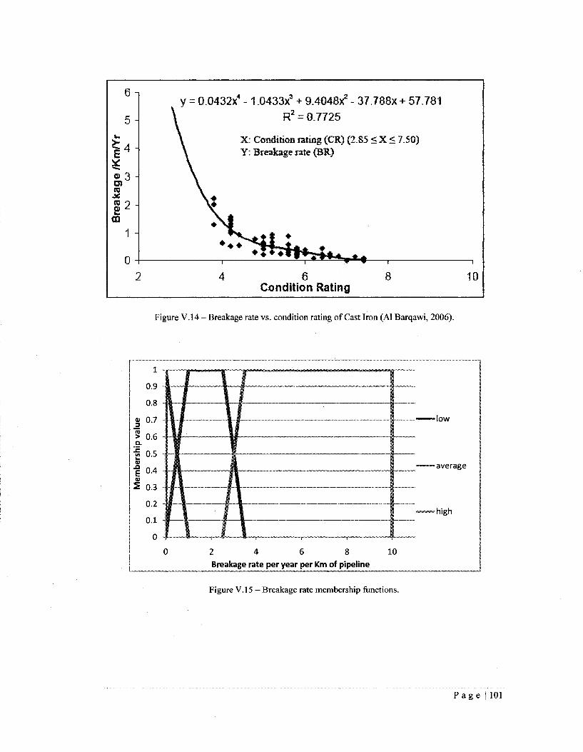
54

© 3 o

CQ

0

y = 0.0432X4 - 1.0433x3 + 9.4048** - 37.788X+ 57.781 R2 = 0.7725

X: Condition rating (CR) (2.85 < X < 7.50) Y: Breakage rate (BR)

Condition Rating 8 10

Figure V.14 - Breakage rate vs. condition rating of Cast Iron (Al Barqawi, 2006).

0.9 -

no .

« 0.7

"5 f l f i -a •5 0.5 -

| 0.4 -01 2 n 3 -

0.2 -

C

i f | ( I f f I f If If I I If | | | |

w w 1 1 n li MM if » l i if • I 1 p H

f i l l I 1 f 1 1 J J 1 1 2 4 6 8

Breakage rate per year per Km of pipeline

_ -

1 I

• |

I jf I

1 I % if

1 1

JfZZ 10

— • l o w

——average

— high

Figure V.l 5 - Breakage rate membership functions.

P a g e | 101

Hydraulic Factor

The hydraulic factor is used to measure the current network performance and is

usually indicated by the C-factor of the pipelines. A preliminary investigation of

the hydraulic capacity of a distribution system can be done by analyzing the

results of low-pressure complaints, hydrant-flow, rusty color occurrence, and

visual inspection of interior pipe tests, which will give the trend of the

distribution system's hydraulic capacity change over time and how it varies

spatially. Detailed investigation of the hydraulic factor is carried out using

Hazen-William factor tests (roughness test) (InfraGuide, 2003). Hydraulic

factor is one of the important factors that give a good indication of the status of

the network, and it is classified according to the Hazen-William factor into five

groups (Al Barqawi, 2006). The membership functions and their characteristics

are shown in Figure V.16. The data type to be used for this factor is the value of

the Hazen-Willam factor with a maximum of 150 (maximum value of a new

installation).

P a g e | 102

1

0.9

0.8

oi 0.7

2 0.6 Q.

1 0.5 01 | 0.4 O)

2 0.3

0.2

0.1 0

Figure V.16 - Hydraulic factor membership functions.

Water Quality

Measuring water quality in the water distribution network gives a good

indication about the internal condition of a pipelines' network. The preliminary

data collected in order to assess the water quality in a distribution system is

based on analyzing the water quality complaint records and the routine water

quality monitoring data. Water quality can be measured based on the

concentrations of chlorine residuals and iron in metallic mains. When chlorine

residuals are decreased in some areas of a water system, it indicates that these

areas are deteriorating. An increasing concentration of iron in the water indicates

the degree of internal corrosion of unlined metallic mains (InfraGuide, 2003). In

this research, water quality is considered as a subjective factor and classified

into five groups: very good, good, acceptable, bad, and very bad. The

membership functions and their characteristics are shown in Figure V.17. The

P a g e | 103

50 100 C-factor

150

data type used for this factor is numerical from 0 to 10 where 0 indicates the best

water quality and 10 indicates the worst water quality.


10

Figure V.17 - Water quality membership functions.

Leakage rate

Leakage in the pipelines indicates the presence of cracks and/or joint failure.

This can give a strong indication about the status of the network. There are many

tests that can assess the network leakage. Hydrostatic leakage tests and water

audits are the most common methods used to detect leakage in the water system

(Al Barqawi, 2006). Leakage erodes pipe bedding and increases soil moisture in

the pipe zone (InfraGuide, 2003). In this research, due to lack of information

about leakage rate evaluation and rating, it is considered as a subjective factor

and classified into five groups: very high, high, medium, low, and very low. The

P a g e | 104

membership functions and their characteristics are shown in Figure V.18. The

data input to be used for this factor is numerical from 0 to 10, where 0 indicates

the least leakage rate and 10 indicates the worst leakage rate.

o 2 4 6 8 10


Figure V.l 8 - Leakage rate membership functions.

V.3.4. Post Failure Model

Estimating the consequences of pipeline failure is a complicated process. A

simplification of the process is sought, therefore, and a qualitative (subjective)

approach rather than a quantitative (objective) approach will be followed. Five

factors are considered in this research: cost of repair, damage to

surroundings/business disruption, loss of production, traffic reduction, and type

of area serviced.

P a g e | 105

Cost of Repair

The cost of repair is the direct cost due to a burst pipeline. However, it is

difficult to comprehend this factor since it varies depending on the magnitude of

failure, the area of failure, time of failure, country of failure, etc

(Bandyopadhyay et al. 1997). The main factors which contribute to the repair

cost are the cost of the repair material and the cost of labor. The cost of repair

material is dependent on the original pipeline material and its characteristics, for

example: steel pipes can be repaired by welding a steel sleeve to the position of

pipeline burst, but it is not applicable to plastic pipes which require another type

of repair material. On the other hand, the cost of labor is dependent on the time

consumed and the number of laborers involved in the repair. In its turn, the time

consumed is dependent on the pipeline cover material and depth, the presence of

other buried utilities such as electricity power lines, telephone lines, gas lines,

etc, the location of the failure (accessibility) (Pickard, 2007). In this research,

cost of repair is classified into five subjective groups (on a scale of 0 to 10) as

very high, high, medium, low, and very low. The membership functions and

their characteristics are shown in Figure V.19. The data type to be used for this

factor is numerical from 0 to 10 where 0 indicates the lowest and 10 indicates

the highest cost of repair.

P a g e | 106

—•—» very low

— l o w

<——medium

high

——very high

10

Figure V.19 - Cost of repair membership functions.

Damage to surroundings/Business Disruption

The most visible impact associated with a water main break is the occurrence of

flooding affecting structures. Flooding causes quantifiable damage to structures

and their contents which is dependent on the specific structure type, value,

regional location and use. The cost associated with flooding is building structure

damage and building content damages and even damage to property surrounding

building such as gardens and sheds (Cromwell et al. 2002). In this research, the

damage to surroundings and business disruption is classified into three groups

according to the location of the pipeline failure as residential, commercial, and

industrial. The membership functions and their characteristics are shown in

Figure V.20. The data type to be used for this factor is linguistic and chosen

from this list: Industrial, Commercial, and Residential.

P a g e | 107

I 1 I * i

i

1 I

, — _ — . - J

Industrial Commercial Residential

 Q.

2S ^ 0 qui

01

s

0.9

0.8

0.7

0.6

0.5

0.4

0.3

0.2

0.1

Figure V.20 - Damage to surroundings membership functions.

Loss of Production

Loss of production means the loss of profit from normal service. Loss of

production is usually dependent on the size of the pipeline, the duration from

time of failure to time of service resumption, and the location of the pipeline and

whether it is redundant or not. Redundancy of the water network is achieved by

duplicating elements in the network in order to eliminate the effects of any

single point of failure. For this reason, the loss of production is classified here

according to pipeline size and redundancy status as small redundant, small not-

redundant, medium redundant, and medium not-redundant. The membership

functions and their characteristics are shown in Figure V.21. The redundant and

not-redundant pipelines share the same membership functions (overlaid each

other). The data type to be used for this factor is pipeline diameter, up to 500

P a g e | 108

millimeters, and the redundancy condition to be chosen from Redundant or Not-

Redundant.

0.9

0.8

0.7

0.6

0.5

0.4

2 0.3

0.2

0.1

Small-Redundant/

Not-Redundant

• medium-Redundant/

Not-Redundant

100 200 300 400

Pipe diameter, mm

500

Figure V.21 - Loss of production membership functions.

Traffic Disruption

In the event of water main failure, mild to severe traffic disruption can occur.

Traffic disruption causes inconveniences for the travelling public and can

disrupt different businesses, in terms of customers and with freight and package

delivery. The cost of traffic disruption is dependent on the increase of travel

time and the value of travel time (Cromwell et al. 2002). However, the value of

travel time is dependent on many factors by its turn. The increase of travel time

is dependent on the type of road and traffic above the failed pipeline. In this

research, a qualitative approach will be followed and traffic disruption as a cost

P a g e | 109

will be classified as a subjective factor into 5 groups as: very disruptive,

disruptive, moderate, light, and very light. The membership functions and their

characteristics are shown in Figure V.22. The data type to be used for this factor

is numerical from 0 to 10, where 0 indicates the least traffic disruption and 10

indicates the highest traffic disruption.

Very light

Light

Moderate

Heavy

Very heavy

Figure V.22 - Traffic disruption membership functions.


In the case of pipeline failure, the water supply will stop serving a targeted

destination. Hence, numerous businesses in the destination area will be

negatively affected by the failure. The end users start to complain when they

don't receive the service they need, which will damage the operator's reputation.

Usually, water main networks are designed in a way to keep delivering water

even if a failure occurs by using other paths (redundancy) (Oppenheimer, 2004).

However, a drop in water pressure is also considered a failure. Depending on the

P a g e | 110

2 4 6 8


11

area serviced, this factor can be classified into residential, commercial, and

industrial (Al Barqawi, 2006). The membership functions and their

characteristics are shown in Figure V.23. The data type to be used for is

linguistic and chosen from this list: Industrial, Commercial, and Residential.

0.9 -

0.8 -

a. 0.7 -3 > 0.6 -Q.

•§ 0.5 -

| 0.4 -

2 0.3 -

0.2 -

0.1 -n •

1 1

Industrial Commercial Residential

Figure V.23 — Type of serviced area membership functions.

V.3.5. Risk of failure Model

This model combines the results of the previous four models to generate the risk

of failure of water main. Thus, the membership functions of the four main

factors (environmental, physical, operational, and post failure) are identical to

the standardized consequent membership functions of the four models (as will

be explained in Section V.5. Consequents Aggregation). It consists of seven

membership functions (extremely low, very low, moderately low, medium,

P a g e | 111

moderately high, very high, and extremely high) on a qualitative scale from 0 to

10 as shown in Figure V.24.

Extremely Low

Very Low

Moderately Low

Medium

Moderately High

Very High

Extremely High

4 6 (0-10) Qualitative Scale

10

Figure V.24 - Fuzzification membership functions of the four main factors in the risk of failure model.

V.4. Fuzzy Inference

In this research, the indirect knowledge acquisition method (by means of a

questionnaire and the available literature) is used to develop the knowledge base

of the risk of water main failure model as shown in IV.1.3. Expert knowledge

base.

The Mamdani fuzzy rules system type is used in the fuzzy model, which has an

advantage over the Takagi-Sugeno-Kang (TSK) method of being easier to

understand and the consequents of the system is defined in terms of fuzzy sets as

explained in Section "A.6.1. Mamdani Method". The Mamdani method is based

on a simple structure of Min operations as follows:

P a g e | 112

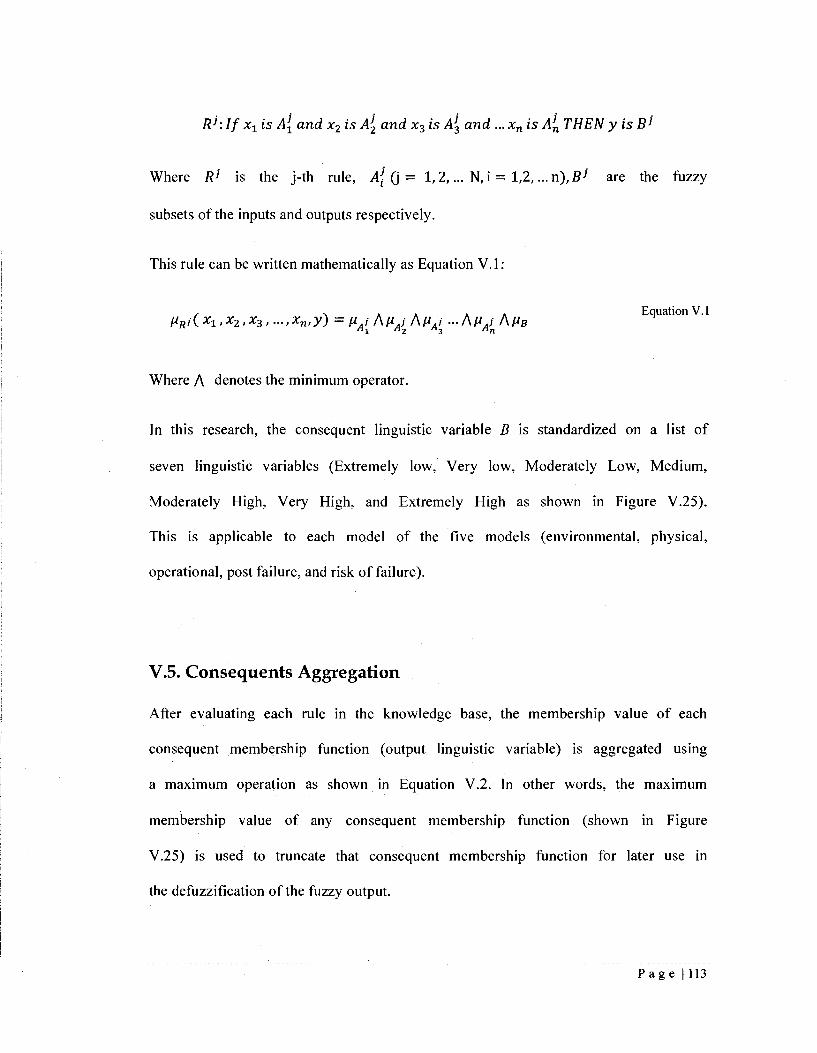
/? ;: If xt is A[ and x2 is A2 and x3 is A3 and ...xn is A]n THEN y is fiJ

Where RJ is the j-th rule, A{ (j = 1,2,... N,i = 1,2, ...n),Bj are the fuzzy

subsets of the inputs and outputs respectively.

This rule can be written mathematically as Equation V.l:

, , . » « « Equation V.l Hi ix1,x2,x3,..., xn, y) = UJ A n.i A HJ ... A ju / A Ms

" l " 2 3 -"n

Where A denotes the minimum operator.

In this research, the consequent linguistic variable B is standardized on a list of

seven linguistic variables (Extremely low, Very low, Moderately Low, Medium,

Moderately High, Very High, and Extremely High as shown in Figure V.25).

This is applicable to each model of the five models (environmental, physical,

operational, post failure, and risk of failure).

V.5. Consequents Aggregation

After evaluating each rule in the knowledge base, the membership value of each

consequent membership function (output linguistic variable) is aggregated using

a maximum operation as shown in Equation V.2. In other words, the maximum

membership value of any consequent membership function (shown in Figure

V.25) is used to truncate that consequent membership function for later use in

the denazification of the fuzzy output.

P a g e | 113

N

Hn(x1,X2,X3,...,Xn,y) = \J[liR)(x1,X2,Xz,...,Xn,y)} Equation V.2

7=1

Where V denotes the maximum operation, R represents each of the consequent

membership functions as standardized to the list of (Extremely low, Very low,

Moderately Low, Medium, Moderately High, Very High, and Extremely High).

This is also applicable to each model of the five models (environmental, physical,

operational, post failure, and risk of failure).

____ Extremely Low

— V e r y Low

—— Moderately Low

——Medium

U "——Moderately High

- - Very High

Extremely High

10 (0-10) Qualitative Scale

Figure V.25 - Consequent membership functions.

V.6. Defuzzification Process

There are many defuzzification methods that convert the fuzzy consequents of

all of the triggered fuzzy rules to a crisp value. The method used in this research

is the Center of Sum as shown in Equation V.3.

P a g e | 114

Crisp Risk Output =

extremely high . extremely high

y Truncated Arean x Centeriodn I y n=extremely low ' n=extreme

Truncated Arean

^extremely low ' n=extremely low

Equation V.3

This equation calculates the center of gravity of each truncated consequent

membership function found from the previous step (neglecting the union

operation) and then average-weights them by their areas. It has the advantage of

being simple to program, requiring less computer resources, and it gives

reasonable results. Section A.7. Defuzzification Methods in Appendix A

contains more information.

This is also applicable to each model of the five models (environmental,

physical, operational, post failure, and risk of failure).

V.7. System Analysis and Verification

Two different approaches are used to test and verify the developed model and system.

The first approach is system sensitivity analysis (stability testing), which tests the effects

of the different factors on the behaviour of the model. The second approach is model

accuracy testing which uses a validated AHP deterioration model to verify the results of

the developed model.

P a g e | 115

V.7.1. Sensitivity Analysis and System Stability Testing

The sensitivity and stability of the model have to be tested in order to insure that the

model is performing as expected under different model parameters. Therefore, several

scenarios are assumed and applied to the model and the results are examined for any

illogicality. The scenarios are as follows:

1. Lowest and highest risk of failure (ID numbers 1 and 2 in Table V.l). By

analyzing the results, the maximum theoretical risk of failure that the model can

generate is 9.4 and the minimum is 0.6. This is due the fact that the method used

in defuzzification is Center of Sum, which calculates the center of the area under

the triangular membership functions and thus limits the risk index to a maximum

of 9.4 and a minimum of 0.6. However, the actual maximum risk of failure that

can be generated by the model is 8.8 and the minimum is 1.7, due to the

behavior of certain physical factors since there is no Extremely High Risk output

membership functions used in the model for the Pipe Diameter and Protection

Method factors, due to the performance conflicts of different factors (e.g.

cathodic protection can not accompany PE or PVC pipes, pipe diameter

performance conflicts with loss of production performance).

2. Sensitivity analysis by increasing the risk of failure values. This is done by

increasing the adverse effect (riskier performance) of the factors (one at a time),

starting from the factor that has the highest weight among the considered factors

and ending with the factor that has the lowest weight (ID number 3 to 112 in

Table V.l and Appendix C). By analyzing this scenario, it is noticeable that the

risk of failure index is changing at a quicker pace in the early stages (for the first

P a g e | 116

factors) and at a slower pace in the later stages (in the last factors) as shown in

Figure V.26. This is due to the fact that the factors with the highest weight are

examined first and the factors with the lowest weights are examined at the end,

where they don't have enough power to make a noticeable change. Figure V.26

shows jump steps in the results. This occurs for several reasons, such as the

change in the factor status alone is not enough to make a change in the final

result. Other reasons are the rules evaluation and aggregation, and the use of the

center of sum defuzzification method.

<L>

01 £ nj -

a

01 Q .

>-t -o

i / i

v- P o ^ Si .2 =3

|5 ] * - _^ » _ — J ft § ro _ _ H _

ro Q

E g

3 f - <

OC

20 40 60 80 100 120 Number of Examined Records

Figure V.26 - Sensitivity analysis of the model.

P a g e | 117

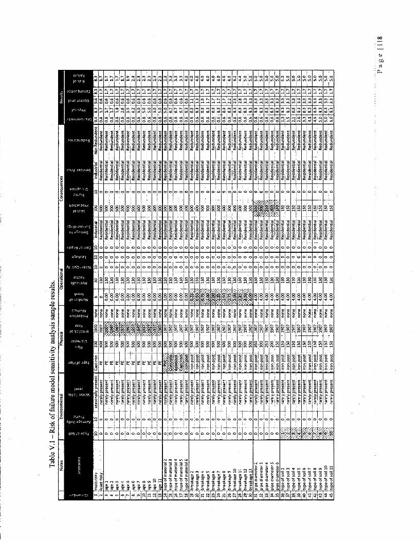
Tab

le V

.l -

Ris

k of

fai

lure

mod

el s

ensi

tivity

ana

lysi

s sa

mpl

e re

sult

s.

Env

iron

men

tal

Con

sequ

ence

s

1 'm

ost r

isky

2

ileas

t ris

ky

3 4 5 e 7 8

ag

el

age

2 ag

e 3

age

4 ag

e 5

age

6 9

:age

7 10

11

12

13

14

~1

5~

16

"l7

~ 18

19

age

8 ag

e 9

age

10

age

11

type

of

mat

eria

! 2

type

of m

ater

ial 3

ty

pe o

f mat

eria

l 4

type

of

mat

eria

l 5

type

of

mat

eria

l 6

brea

kage

2

20 [

brea

kage

3

21

22

23

24

25

26

27

28

29

Id

31

brea

kage

4

brea

kage

5

brea

kage

6

brea

kage

7

brea

kage

8

brea

kage

9

brea

kage

10

brea

kage

11

brea

kage

12

brea

kage

13

pipe

dia

met

er 2

32

jpi

pe d

iam

eter

3

33

"34 35

36

37

38

39

40

41

42

43

44

45

pipe

dia

met

er 4

pi

pe d

iam

eter

5

pipe

dia

met

er 6

ty

pe o

f so

il 2

type

of s

oil 3

ty

pe o

f soi

l 4

type

of s

oil 5

ty

pe o

f soi

l 6

type

of s

oil 7

ty

pe o

f so

il 8

type

of s

oil 9

ty

pe o

f soi

l 10

type

of

soil

11

10

0 0 0 0 0 0 0 0 0 0 0 0 0 0 0 0 0 ° 0 0 0 0 0 0 0 0 0 -h

0 0 -f- 3 * s 8 9 10

10

0 0 0 0 0 0 0 0 0 0 0 0 0

....

.. 0 0 0 0 0 0 0 0 0 0 0 0 0 0 0 0 0 0 0 0 0 0 0 0 0 0 0 0 0 0

seas

onal

ly p

rese

nt

rare

ly p

rese

nt

rare

ly p

rese

nt

rare

ly p

rese

nt

L ra

rely

pre

sent

_̂_

ra

rely

pre

sent

ra

rely

pre

sent

ra

rely

pre

sent

ra

rely

pre

sent

ra

rely

pre

sent

ra

rely

pre

sent

ra

rely

pre

sent

ra

rely

pre

sent

ra

rely

pre

sent

ra

rely

pre

sent

ra

rely

pre

sent

ra

rely

pre

sent

ra

rely

.pre

sent

ra

rely

pre

sent

ra

rely

pre

sent

ra

rely

pre

sent

ra

rely

pre

sent

ra

rely

pre

sent

ra

rely

pre

sent

ra

rely

pre

sent

ra

rely

pre

sent

ra

rely

pre

sent

ra

rely

pre

sent

ra

rely

pre

sent

ra

rely

pre

sent

ra

rely

pre

sent

ra

rely

pre

sent

ra

rely

pre

sent

ra

rely

pre

sent

ra

rely

pre

sent

ra

rely

pre

sent

ra

rely

pre

sent

ra

rely

pre

sent

ra

rely

pre

sent

ra

refy

pre

sent

ra

rely

pre

sent

ra

rely

pre

sent

ra

rely

pre

sent

ra

rely

pre

sent

ra

rely

pre

sent

Cas

t iro

n PE

PE

PE

PE

PE

PE

PE

PE

PE

PE

PE

PE

^_

PV

C__

^ C

oncr

ete

Asb

esto

s C

ast I

ran

: iro

n po

st

: iro

n po

st

; iro

n po

st

: iro

n po

st

: iro

n po

st

: iro

n po

st

: iro

n po

st

: iro

n po

st

: iro

n po

st

: iro

n po

st

: iro

n po

st

: iro

n po

st

.iro

n po

st

: iro

n po

st

: iro

n po

st

: iro

n po

st

: iro

n po

st

:iro

n po

st

: iro

n po

st

; iro

n po

st

: iro

n po

st

: iro

n po

st

: iro

n po

st

: iro

n po

st

: iro

n po

st

:iro

n po

st

: iro

n po

st

: iro

n po

st

100

500

500

500

500

500

500

500

500

500

500

500

500

500

500

500

1 50

0 ""•

50

0 50

0 50

0 50

0 50

0 50

0 50

0 r

500

500

L_

50

0 ,5

00

500

500

350

300

250

^2

00

150

150

r 15

0 15

0 15

0 IS

O

150

150

150

150

150

1900

20

07

2007

,-1

997

1987

13

77

1967

19

S7

1947

19

37

1927

•1

917

1907

19

07

1907

19

07

1907

19

07

1907

19

07

1907

19

07

1907

19

07

1907

19

07

1907

19

07

1907

19

07

1907

^1

90

7 19

07

1907

19

07

,_19

07

1907

19

07

1907

19

07

1907

19

07

1907

19

07

1907

none

no

ne

none

no

ne

none

no

ne

none

no

ne

none

no

ne

none

no

ne

none

no

ne

none

no

ne

none

no

ne

none

no

ne

none

no

ne

none

no

ne

non*

-no

ne

nonf

no

nt

nont

no

ne

nonf

no

nt

none

no

ne

none

no

ne

none

no

ne

none

no

ne

none

no

ne

none

no

ne

none

6 0 0.

00

0.00

0.

00

0.00

0.

00

0.00

0.

00

0.00

0.

00

0.00

0.

00

0.00

0.

00

0.00

0.

00

0.00

0.

25

0.50

0.

75

1.00

2.

00

;?5

2 50

2

75

3 00

3

25

3 50

4

00

4 00

41

..J

4.00

4.

00

4.00

4.

00

4.00

4.

00

4.00

4.

00

4.00

4.

00

4.00

4.

00

4.00

30

130

130

130

130

130

130

130

130

130

130

130

130

130

130

130

130

130

130

130

130

130

130

130

130

130

130

130

130

130

130

130

130

130

130

130

130

130

130

130

130

130

130

130

130

HP

0 0 0 0 0 0 0 0 0 0 0 0 0 0 0 0 0 0 0 0 0 0 0 0 0 0 0 0 0 0 0 0 0 0 0 0 0 0 0 0 0 0 0 0

10

0 0 0 0 0 0 0 0 0 0 0 0 0 0 0 0 0 0 0 0 0 0 0 0 0 0 0 0 0 0 0 0 0 0 0 0 0 0 0 0 0 0 0 0

10

0 0 0 0 0 0 0 0 0 0 0 0 0 0 0 0 0 0 0 0 0 0 0 0 0 0 0 0 0 0 0 0 0 ° 0 0 0 0 0 0 0 0 0 0

Indu

stria

l R

esid

entia

l R

esid

entia

l R

esid

entia

l R

esid

entia

l R

esid

entia

l R

esid

entia

l R

esid

entia

l R

esid

entia

l R

esid

entia

l R

esid

entia

l R

esid

entia

l R

esid

entia

l R

esid

entia

l R

esid

entia

l R

esid

entia

l R

esid

entia

l R

esid

entia

l R

esid

entia

l R

esid

entia

l R

esid

entia

l R

esid

entia

l R

esid

entia

l R

esid

entia

l R

esid

entia

l R

esid

entia

l R

esid

entia

l R

esid

entia

l R

esid

entia

l R

esid

entia

l R

esid

entia

l R

esid

entia

l R

esid

entia

l R

esid

entia

l R

esid

entia

l R

esid

entia

l R

esid

entia

l R

esid

entia

l R

esid

entia

l R

esid

entia

l R

esid

entia

l R

esid

entia

l R

esid

entia

l R

esid

entia

l R

esid

entia

l

100

500

500

500

500

500

500

500

500

500

500

500

500

500

500

500

500

500

500

500

500

500

500

5O0

500

500

500

500

500

500

, 35

0 30

0 25

0 •

200

150

150

150

150

150

150

ISO

15

0 15

0 15

0 15

0

10

0 0 0 0 0 0 0 0 0 0 0 0 0 0 0 0 0 0 0 0 0 0 0 0 0 0 0 0 0 0 0 0 0 0 0 0 0 0 0 0 0 0 0 0

Indu

stria

l R

esid

entia

l R

esid

entia

l R

esid

entia

l R

esid

entia

l R

esid

entia

l R

esid

entia

l R

esid

entia

l R

esid

entia

l R

esid

entia

l R

esid

entia

l R

esid

entia

l R

esid

entia

l R

esid

entia

l R

esid

entia

l R

esid

entia

l R

esid

entia

l R

esid

entia

l R

esid

entia

l R

esid

entia

l R

esid

entia

l R

esid

entia

l R

esid

entia

l R

esid

entia

l R

esid

entia

l R

esid

entia

l R

esid

entia

l R

esid

entia

l R

esid

entia

l R

esid

entia

l R

esid

entia

l R

esid

entia

l R

esid

entia

l R

esid

entia

l R

esid

entia

l R

esid

entia

l R

esid

entia

l R

esid

entia

l R

esid

entia

l R

esid

entia

l R

esid

entia

l R

esid

entia

l R

esid

entia

l R

esid

entia

l R

esid

entia

l

Not

Red

unde

nt

Red

unde

nt

Red

unde

nt

Red

unde

nt

Red

unde

nt

Red

unde

nt

Red

unde

nt

Red

unde

nt

Red

unde

nt

Red

unde

nt

Red

unde

nt

Red

unde

nt

Red

unde

nt

Red

unde

nt

Red

unde

nt

Red

unde

nt

Red

unde

nt

Red

unde

nt

Red

unde

nt

Red

unde

nt

Red

unde

nt

Red

unde

nt

Red

unde

nt

Red

unde

nt

Red

unde

nt

Red

unde

nt

Red

unde

nt

Red

unde

nt

Red

unde

nt

Red

unde

nt

Red

unde

nt

Red

unde

nt

Red

unde

nt

Red

unde

nt

Red

unde

nt

Red

unde

nt

Red

unde

nt

Red

unde

nt

Red

unde

nt

Red

unde

nt

Red

unde

nt

Red

unde

nt

Red

unde

nt

Red

unde

nt

Red

unde

nt

9.4

0.6

0.6

0.6

0.6

0.6

0.6

0.6

0.6

0.6

0.6

0.6

0.6

0.6

0.6

0.6

0.6

0.6

0.6

0.6

0.6

0.6

0.6

0.6

0.6

0.6

0.6

0.6

0.6

0.6

0.6

0.6

0.6

0.6

0.6

1.3

1.5

2.1

2.6

3.3

4.1

4.5

5.0

5.0

5.0

83

1.7

1.7

1.7

1.8

2.6

3.5

4.2

5,0

5.0

5.0

5.0

5.0

5.0

6.7

6.7

6.7

8.3

8.3

8.3

8.3

8.3

8.3

8.3

8.3

8.3

8.3

8.3

8.3

8.3

8.3

8.3

8.3

8.3

8.3

8.3

8.3

8.3

8.3

8.3

8.3

8.3

8.3

8.3

8.3

"57

0.6

0.6

0.6

0.6

0.6

0.6

0.6

0.6

0.6

0.6

0.6

0.6

0.6

0.6

0.6

0.6

0.6

1.1

1.3

1.5

1.7

1.7

1.7

1.7

2.2

2.5

2.8

3.3

3.3

3.3

3.3

3.3

3.3

3.3

3.3

3.3

3.3

3.3

3.3

3.3

3.3

3.3

3.3

3.3

riT

1.

7 1.

7 1.

7 1.

7 1.

7 1.

7 1.

7 1.

7 1.

7 1.

7 1.

7 1.

7 1.

7 1.

7 1.

7 1.

7 1.

7 1.

7 1.

7 1.

7 1.

7 1.

7 1.

7 1.

7 1.

7 1.

7 1.

7 1.

7 1.

7 1.

7 1.

7 1.

7 1.

7 1.

7 1.

7 1.

7 1.

7 1.

7 1.

7 1.

7 1.

7 1.

7 1.

7 1.

7

£3

1.7

1.7

1.7

1.7

1.7

1.9

2.4

2.3

2.3

2.3

2.3

2.3

2.3

3.3

3.3

3.3

4.0

4.0

4.0

4.0

4.0

4.0

4.0

4.0

4.0

4.2

4.4

5.0

5.0

5.0

5.0

5.0

5.0

S.0

5.

0 5.

0 5.

0 5.

0 5.

0 5.

0 5.

0 5.

0 s.o

5.0

Pa

ge

I 118

3. Close testing of the factor that has the highest weight in the physical model. This

is the Age factor at an increment of 10 years, as shown in Table V.l. Analyzing

the results, which tests the Age factor (fixing the rest of the physical factors at

medium consequents) and draws a curve for the physical risk values (Figure

V.27), it shows a steady stage at the start (10 to 30 years) and at the end (50 to

80 years) and a smooth increasing stage in the middle of the curve (30 to 50

years). This is because the model maps five input membership functions in this

factor to seven output membership functions which will cause unevenly

distributed results (two close membership functions at the beginning and two at

the end of the curve and one membership function in the middle of the curve).

However, by analyzing the effect of age factor on the risk of failure values, one

can observe that it is difficult to make a change in the risk of failure value by

only changing the performance of one factor, since the other fifteen factors try to

resist the change in the risk values, as shown in Figure V.26. Testing the Age

factor when the other factors are absent will give an indication of how the

system performs when there is no resistance from other factors. Figure V.28

shows a graph of the physical index of the age factor alone. The stable part at the

very end of the graph is due to the shape of the fuzzy membership functions of

the age factor (a trapezoidal membership function).

P a g e | 119

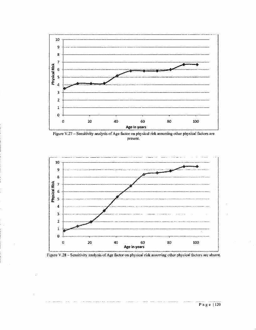
Figure V.27 — Sensitivity analysis of Age factor on physical risk assuming other physical factors are present.

Figure V.28 - Sensitivity analysis of Age factor on physical risk assuming other physical factors are absent.

P a g e | 120

4. Close testing the physical model (chosen here because the two factors under

study are parts of this model) and risk of failure model sensitivity towards

change in the consequents of the two highest weighted factors (Age and Pipe

material). This is done through three scenarios by fixing the values of the other

physical factors at the medium consequents (all other physical factors are

present), at the highest risk consequents, and at the lowest risk consequents, and

at the same time changing the values of the factors under study from lowest to

highest risks consequents (Table V.2). Analyzing the results of physical model

sensitivity towards the age and pipe material factors and analyzing Figure V.29,

Figure V.31, and Figure V.32, it is obvious that the physical model is more

sensitive toward the age factor (which has the highest weight) since it causes a

change in the physical risk at medium risk level from 3.5 to 6.7 with a steeper

curve (compared to the other factor, pipe material). However, the pipe material

factor causes a change in the physical risk at medium risk level from 4.2 to 6.0

with a smoother curve. Figure V.30 shows that due to the very close weights of

the age and pipe material factors (30 and 40), the risk of failure model has the

same sensitivity towards these two factors where they both cause a change in

failure risk value from 5.0 to 5.8. As a result, each of the four models

(environmental, physical, operational, and post failure) is more sensitive to its

own factors than the risk of failure model is. This fact is due to the use of a

hierarchical system where the farther the factor is in the hierarchy, the less its

effectiveness (sensitivity) to the top level model is.

P a g e | 121

Table V.2 - Physical and risk of failure models sensitivity analysis of age and pipe material factors.

ID n

umbe

r

1

2

3

4

5

6

7

8

9

10

11

12

13 14

15

16

17 18 19 20

21

22

23 24

25

26 27

28 29 30

Scen

ario

s

be E

2

-c X

.12 ix

o _ j

Factors under study

agel

age 2

age 3

age 4

age 5

type of material 1

type of material 2

type of material 3

type of material 4

type of material 5

agel

age 2

age 3

age 4

age 5

type of material 1 type of material 2 type of material 3 type of material 4 type of material 5

agel

age 2

age 3

age 4

age 5

type of material 1 type of material 2 type of material 3 type of material 4 type of material 5

Type

of

Pipe

Concrete

Concrete

Concrete

Concrete

Concrete

PE

PVC

Concrete

Asbestos

Cast iron post war

Cast iron post war

Cast iron post war

Cast iron post war

Cast iron post war

Cast iron post war

PE

PVC

Concrete Asbestos

Cast iron post war

PE

PE

PE

PE

PE

PE PVC

Concrete Asbestos

Cast iron post war

Pipe

D

iam

eter

250

250

250

250

250

250

250

250

250

250

50

50

50

50

50

50 50 50 50 50

500

500

500

500

500

500 500

500 500 500

Inst

alla

tion

Y

ear

2007

1982

1957

1932

1907

1967

1967

1967

1967

1967

2007

1982

1957

1932

1907

1900 1900 1900 1900 1900

2007

1982

1957

1932 1907

2007 2007

2007 2007 2007

Pro

tect

ion

M

eth

od

none

none

none

none

none

none

none

none

none

none

none

none

none

none

none

none none none none none

Lining\Coating

Lining\Coating

Lining\Coating

Lining\Coating

Lining\Coating

Lining\Coating Lining\Coating

Lining\Coating Lining\Coating Lining\Coating

Phys

ical

Ris

k

3.5

4.2

5.8

6.0

6.7

4.2

4.3

5.2

5.8

6.0

5.0

5.6

7.6

8.3

8.3

6.7 6.7 6.7 8.3 8.3

0.7

1.7

2.6

3.3

3.3

0.7 1.7

1.7 1.8 3.3

Risk

of

Failu

re

5.0

5.0

5.4

5.8

5.8

5.0

5.0

5.4

5.8

5.8

7.7

7.7

8.3

8.3

8.3

8.3 8.3 8.3 8.3 8.3

1.3

1.7

1.7

1.7

1.7

1.3 1.7 1.7 1.7 1.7

P a g e | 122

! '

1957

1907

m „** — W * ' * ^ ^ Asbestos C a s t l r o n

*" ^ " ^ Post Wa r

PE

2007

PVC s^^*'0'^ Concrete

1982

• Age

• Pipe Material - - - • Poly. (Age) — — Poly. (Pipe Material)

Figure V.29 - Physical model sensitivity analysis of age and pipe material factors at medium risk level.

10

9

8

7 01

| 6 '5 "•'5 o -3U he

3

2

1

0

PE

2007

Asbestos Cast Iron Postwar

PVC

1982

Concrete

1 9 5 7

^mm^^^^^W

1932 1907

Age

Pipe Material

Figure V.30 - Risk of failure model sensitivity analysis of age and pipe material factors at medium risk level.

P a g e | 123

9 -

8 -

7 2

.a A

> f 4

3 -

2

1 -

n -

]

PE PVC

2007 1982

1957

Concrete

1932 1907

•*" Asbestos Cast Iron Postwar

L 2 3 4 5

Figure V.31 - Physical model sensitivity analysis of age and pipe material factors at high risk level.

10

9

8

7

1 6

£ 4

3

1932 1907

" " PVC PF

1 9 5 7 — — » — - T <

_ « . - •"• - » « * ' * ' * * * 2 | PE . . - • i r - " * - — " ^ ::Z:ZZI3:r =^— Cast Iron 1 )r . ^ ^ d 1 9 g 2 Concrete Asbestos — P o s t W a r

0 I 2007 _ _ _ . ___, , ,

1 2

Figure V.32 — Physical model sensitivity analysis of age and pipe material factors at low risk level.

5. Close testing of the sensitivity of the physical and risk of failure models toward

the weights of the two most-weighted factors (age and pipe material) within two

times their standard deviation. This will examine the effect of the standard

P a g e | 124

deviation and the change of the mean values. The mean weight of the age factor

is 40 with a standard deviation of 16, whereas the mean weight of pipe material

is 30 with a standard deviation of 12. This test is performed by fixing the values

of the other factors at their least risky effect and fixing the value of the factor

under study at its most risky effect in order to get the most sensitive case. After

that, the test is conducted by changing the value of the weight within the

associated standard deviation (from different expert opinions as shown in Table

IV. 1) at steps of five units and then calculating the physical and risk of failure

values as shown in Table V.3. Analyzing the results of this scenario as shown in

Table V.3, Figure V.33, and Figure V.34, it can be deduced that the physical

model is not very sensitive to the weight of the examined factors within the

factors' standard deviations. Changing the weight of the age factor will cause a

change in the physical risk from 3.3 to 5.0 and the change in pipe material

weight will also make a change from 3.3 to 5.0. The change of the value of the

weight from (n — a) to (jU + o) will result in only 1.7 units of difference which

is not a large difference. This is because of the presence of other factors that act

as resistances to the change in the risk values. Figure V.33 shows that the

physical model starts to be sensitive toward the change in age factor weight

when the weight is reduced below 30. However, the physical model shows more

sensitivity toward the pipe material weight, as shown in Figure V.34, which can

be attributed to the rules evaluation and aggregation, and to the defuzzification

process of the fuzzy output which results in steps in the output, as shown above

in the second sensitivity scenario (Figure V.26). In addition, the risk of failure

P a g e | 125

model shows low sensitivity to the change of the weight of the age and pipe

material as the risk of failure changes from 1.7 to 3.3 in the case of age factor

and 1.7 to 2.3 for pipe material factor, as shown in Table V.3 and Figure V.35.

Table V.3 - Sensitivity analysis of physical and risk of failure models.

ID n

umbe

r

1 2 3 4 5 6 7 8 9 10 11 12 13

14 15 16 17 18 19 20 21 22 23 24

Scenarios

Age weight = 8 Age weight = 15 Age weight = 20 Age weight = 25 Age weight = 30 Age weight = 35 Age weight = 40 Age weight = 45 Age weight = 50 Age weight = 55 Age weight = 60 Age weight = 65 Age weight = 72

Pipe material weight = 6 Pipe material weight = 10 Pipe material weight = 15 Pipe material weight = 20 Pipe material weight = 25 Pipe material weight = 30 Pipe material weight = 35 Pipe material weight = 40 Pipe material weight = 45 Pipe material weight = 50 Pipe material weight = 54

Phys

ical

Ris

k

3.3 3.3 3.3 3.3 5.0 5.0 5.0 5.0 5.0 5.0 5.0 5.0 6.7 1.8 3.3 3.3 3.3 3.5 3.5 5.0 5.0 5.0 5.0 5.0

Ris

k o

f Fa

ilure

1.7 1.7 1.7 1.7 2.3 2.3 2.3 2.3 2.3 2.3 2.3 2.3 3.3 1.7 1.7 1.7 1.7. 1.9 1.9 2.3 2.3 2.3 2.3 2,3

P a g e | 126

10

in 6

. > If 4

Mean - 2 x Standard deviation

Mean -Standard deviation

10

Mean Mean + Standard deviation

20 30 40 50 Factor Weight

60

Mean + 2 x Standard deviation

70 80

Figure V.33 - Physical model sensitivity analysis toward age factor weight.

10

1/1 6

3

2

1

0

Mean - 2 * Standard deviation

Mean-Standard deviation

10 20

Mean Mean + Standard deviation

30 Factor Weight

40

Mean + 2 x Standard deviation

50 60

Figure V.34- Physical model sensitivity analysis toward pipe material weight.

P a g e | 127

10 -

9

a -J

| 6 -'in

o in 4

3 -

2 H

1 -

0 -

(

• * " " * rf^**^ ™ ™ ~ " * " " ~

— — Pipe Material

Age

&*

1

) 10 20 30 40 50 Global weights of factros

60 70 80

Figure V.35 - Risk of failure model sensitivity analysis toward age and pipe material weights.

6. Close testing of the sensitivity of the physical model toward the assumed value

of pipe material certainty 95%. Certainty here refers to the level of confidence in

the consequent part of the pipe material factor as an individual factor, as shown

in Section V.3.2. Physical. This scenario is carried out by changing the certainty

level from 50% to 100%. The data assumed in assessing this scenario and the

differences between the assumed certainty level of 95% and varying certainty

levels at 50%, 75%, and 100% are evaluated as shown in Table V.4. By

analyzing these differences, it can be noticed that these values are very small and

negligible. The reason behind these small differences can be attributed to many

facts related to the use of the certainty level in the model. For instance, the

certainty level (membership value) of the pipe material factor is not important

unless it is the lowest membership value in the triggered rule compared to the

P a g e | 128

other membership valued collected from other physical factors in that rule, as

minimum value is used among them (an AND operation that combines the

physical factor in the knowledge rule). Moreover, the rules evaluation and

aggregation and defuzzification process will reduce even more the effect of the

change in certainty level of the pipe material. The maximum difference recorded

is 0.0439 which is so small that it can be neglected. As a conclusion, the

physical model (and other models in general) is not sensitive to the certainty

level value of the pipe material, which is the second most important factor

among the sixteen factors.

As a result of the analysis conducted here before, the model(s) is sound, stable, and

performs as expected without any irregular, illogic results.

V.7.2. Verification of the Developed Model

In order to verify the developed model, different approaches can be used. Experts' testing

and feedback is one approach. Another approach is to compare the model results to the

results of another related and validated model (Shaheen, 2005). In this context, the

second approach will be used, which is comparing the results of the proposed model with

another model output. The most relevant model to compare to the proposed model is the

AHP model developed by Al Barqawi (2006). However, some points should be kept in

mind when examining the results:

P a g e | 129

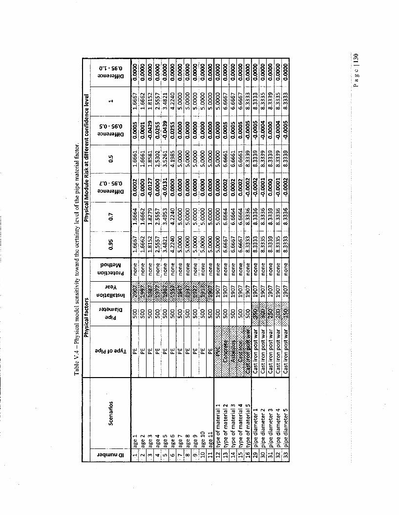
Tab

le V

.4 -

Phys

ical

mod

el s

ensi

tivity

tow

ard

the

cert

aint

y le

vel

of th

e pi

pe m

ater

ial

fact

or.

ID number

1 2 3 4 5 6 7 8 9 10

11

12

13

14

15

16

29

30

31

32

33

Sce

nari

os

age

1 ag

e 2

age

3 ag

e 4

age

5 ag

e 6

age

7 ag

e 8

age

9 ag

e 10

ag

e 1

1

typ

e o

f m

ate

ria

l 1

typ

e o

f m

ate

ria

l 2

typ

e o

f m

ate

ria

l 3

typ

e o

f m

ate

ria

l 4

typ

e o

f m

ate

ria

l 5

pip

e d

iam

ete

r 1

pipe

dia

me

ter

2 pi

pe d

iam

ete

r 3

pipe

dia

me

ter

4 pi

pe d

iam

ete

r 5

Phy

sica

l fac

tors

0>

Q.

a.

**• o 01

a.

> PE

PE

PE

PE

PE

PE

PE

PE

PE

PE

PE

PV

C

Con

cret

e A

sbes

tos

Cas

t ir

on

Cas

t ir

on

po

stw

ar

Ol

E

re

5

50

0 5

00

50

0 5

00

50

0 5

00

50

0 5

00

50

0 5

00

50

0

50

0 5

00

50

0 5

00

500"

c o •5

w

re

nj

= 01

re

>.

20

07

19

97

19

87

19

77

19

67

19

57

19

47

19

37

1927

1917

1

90

7 19

07

1907

1907

19

07

1907

C

ast

iro

n po

st w

ar

| 3

50

' 19

07

Cas

t ir

on

post

wa

r I

30

0 .

1907

C

ast

iro

n po

st w

ar

| 2

50

' 19

07

Cas

t ir

on

post

wa

r C

ast

iro

n po

st w

ar

20

0

"15

0"

" 19

07

1907

c O

TO

••5

O

u

f 0>

4-

> *S

O

)

2 2

a.

no

ne

no

ne

no

ne

no

ne

no

ne

no

ne

no

ne

no

ne

no

ne

no

ne

no

ne

no

ne

no

ne

no

ne

no

ne

no

ne

no

ne

no

ne

no

ne

no

ne

no

ne

Phy

sica

l M

od

ule

Ris

k a

t d

iffe

ren

t co

nfi

de

nce

le

vel

0.95

1.66

67

1.66

62

1.81

52

2.55

57

3.4

82

1

4.22

40

5.00

00

5.0

00

0 5

.00

00

5.0

00

0 5.

0000

5

.00

00

6.66

67

6.66

67

6.66

67

8.33

33

8.33

33

8.33

35

8.33

39

8.33

35

8.33

33

0.7

1.6

66

4

1.6

66

2

1.8

27

9

2.5

55

7 3

.49

53

4.2

24

0 5

.00

00

5.0

00

0 5

.00

00

5.0

00

0

5.0

00

0 5

.00

00

6.6

66

4

6.6

66

4 6

.66

64

8.3

33

6 8

.33

36

8.3

33

6 8

.33

39

8.3

33

6 8

.33

36

=

o

£ •

a o

0.0

00

2 0

.00

00

-0.0

127

0.0

00

0 -0

.01

31

0.0

00

0 0

.00

00

0.0

00

0 0

.00

00

0.0

00

0 0

.00

00

0.0

00

0 0

.00

02

0.0

00

2 0

.00

02

-0.0

00

2 -0

.00

02

-0.0

00

1

0.0

00

0 -0

.00

01

-0.0

002

0.5

1.6

66

1

1.6

66

1

1.8

58

1

2.53

02

3.5

26

1

4.19

85

5.0

00

0 5

.00

00

5.0

00

0 5

.00

00

5.0

00

0

5.0

00

0 6

.66

61

6.6

66

1 6

.66

61

8.3

33

9 8

.33

39

8.3

33

9 8

.33

39

8.3

33

9 8.

3339

g m

c

d Si

T

at

in

*:

°i

S

°

0.00

05

0.0

00

1 -0

.042

9 0.

0255

-0

.043

9 0.

0255

0

.00

00

0.0

00

0 0

.00

00

0.0

00

0 0

.00

00

0.0

00

0 0.

0005

0.

0005

0.

0005

-0

.000

5 -0

.000

5 -0

.000

4 0

.00

00

-0.0

004

-0.0

005

1

1.6

66

7

1.6

66

2

1.8

15

2

2.5

55

7 3

.48

21

4.2

24

0 5

.00

00

5.0

00

0

5.0

00

0 5

.00

00

5.0

00

0

5.0

00

0 6

.66

67

6.6

66

7 6

.66

67

8.3

33

3 8

.33

33

8.3

33

5 8

.33

39

8.3

33

5 8

.33

33

S q

s

?

| S

5

o

0.00

00

0.0

00

0 0.

0000

0.

0000

0.

0000

0.

0000

0

.00

00

0.00

00

0.0

00

0 0.

0000

0.0

00

0 0.

0000

0

.00

00

0.0

00

0 0

.00

00

0.00

00

0.00

00

0.00

00

0.00

00

0.00

00

0.0

00

0

- The AHP model is a deterministic model and does not consider the uncertainty in

the water main performance as the proposed model does.

- Due to the defuzzification process and the characteristics of the fuzzy expert

system, the results of the proposed model may show step results as explained in

section V.7.1. Sensitivity Analysis and System Stability Testing.

- The AHP model only considers deterioration factors and not the consequences

(post failure factors), limiting the accuracy test to only the deterioration factors of

the proposed model. However, the results of this test can be generalized to the

whole proposed model since same approach is used to develop the other factors

that are not examined in this test.

- The AHP model is also based on experts' opinions and experience and

consequently the results are expected to be close to those of the fuzzy expert

system, but not exactly the same since the experts' feedback may differ on the

basis of location, serving period, questionnaire interpretation,... etc.

Two data sets are used to carry out the test: 500 Moncton data points and 1704 London

data points.

- The Moncton data is selected randomly from the data set explained in section

1V.2.1. Data Set One. Some data points, which have characteristics not valid in

AHP model, are excluded from the test. The factors included in this test are: pipe

material, pipe diameter, installation year, protection method, number of breaks,

and hydraulic factor (Hazen-William coefficient). The testing data set is first

evaluated using the proposed fuzzy expert model and then evaluated using the

AHP model. Sample results are shown in Table V.5.

P a g e | 131

Table V.5 - Sample Moncton testing results. H I I H H I I ^ I i l ^ l ^ H ^ ^ ^ ^ ^ S l ^ ^ ^ ^ ^ ^ H ^ l ^ ^ ^ ^ ^ ^ ^ ^ ^ ^ ^ l Proposed model

ID Pipe Material Pipe Dia Year Protection Break Hydraulic Risk Index Output 1 vaiue I abs%-agej AIP

i

2

3

4

5

6

7

8

9

10

11

12

13

14

15

16

17

18

19

20

21

Asbestos Asbestos

Asbestos

Asbestos

Asbestos

Asbestos

Asbestos

Asbestos

Asbestos

Asbestos

Asbestos

Asbestos

Asbestos

Asbestos Asbestos

Asbestos

Asbestos

Asbestos Cast iron

Cast iron

Cast iron

152.4 304.8

152.4

203.2

152.4

304.8

152.4

152.4

152.4

254

254

152.4

152.4

152.4 152.4

152.4

152.4

152.4

254

152.4

254

1959 1959

1959

1959

1959

1959

1959

1959

1959

1959

1959

1959

1959

1959

1959 1964

1959 1959 1920

1909

1943

none

none

none

none

none

none

none

none

none

none

none

none

none

none none

none

none none

none

none

none

0.47

0.22

0.73

0.25

0.13

0.12

0.17

0.00

0.33

0.26

0.40

0.00

0.30

0.35

0.00

0.30

0.25 0.10 0.95

0.65

0.26

74

74

74

74

74

74

74

74

74

74

74

74

74

74 74

79

74 74

35

24

58

4.9 4.2

5.3

4.3

4.9

4.1

4.9

4.8

4.9

4.2

4.4

4.8

4.9

4.9

4.8

4.9

4.9

4.9

7.5

7.1

5.8

4.4

4.3

4.8

4.4

4.1

3.9

4.1

3.4

4.4

4.3

4.3

3.4

4.4

4.4

3.4

3.9

4.4 3.7

5.6

6.1

4.0

0.5 9% 0.10

-0.1 1% 0.01

0.4 8% 0.09

-0.1 3% 0.03

0.8 16% 0.20

0.2 5% 0.06

0.8 16% 0.19

1.4 29% 0.42

0.4 9% 0.10

0.0 1% 0.01

0.1 3% 0.03

1.4 29% 0.42

0.4 9% 0.10

0.4 9% 0.10

1.4 29% 0.42

1.0 21% 0.26

0.4 9% 0.10 1.2 24% 0.31

1.9 25% 0.33

1.0 15% 0.17

1.8 31% 0.44

In order to judge whether the model is verified or not when using results

comparison as is the case here, two terms can be used to determine the validity of

the model, Average Validity Percent {AIP) and Average Invalidity Percent (AIP).

A VP represents the validation percent out of 100 and AIP represents the prediction

error (Zayed and Halpin, 2005). These two terms are shown in Equation V.4 and

Equation V.5.

AIP i=l

*-[% / " Equation V.4

AVP = 1-AIP Equation V.5

Where

AIP : Average Invalidity Percent

AVP : Average Validity Percent

Et : Estimated value

Ct : Actual value

P a g e | 132

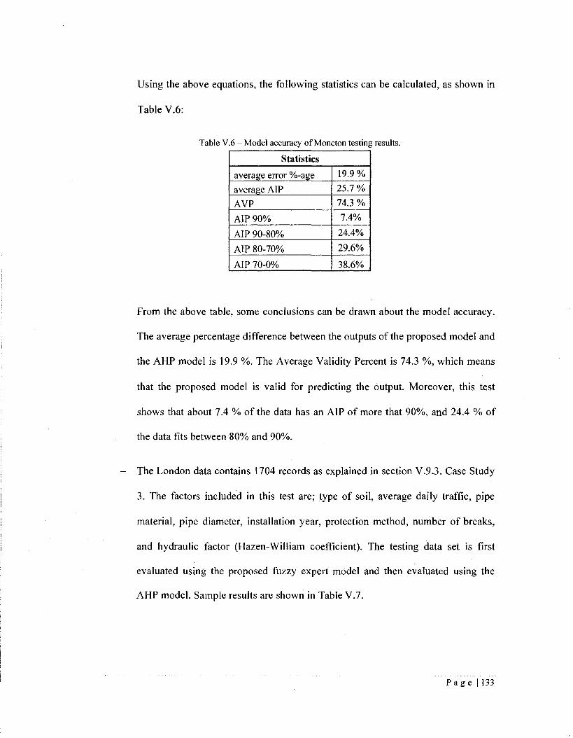
Using the above equations, the following statistics can be calculated, as shown in

Table V.6:

Table V.6 - Model accuracy of Moncton testing results.

Statistics

average error %-age

average AIP

AVP

AIP 90%

AIP 90-80%

AIP 80-70%

AIP 70-0%

19.9%

25.7 %

74.3 %

7.4%

24.4%

29.6%

38.6%

From the above table, some conclusions can be drawn about the model accuracy.

The average percentage difference between the outputs of the proposed model and

the AHP model is 19.9 %. The Average Validity Percent is 74.3 %, which means

that the proposed model is valid for predicting the output. Moreover, this test

shows that about 7.4 % of the data has an AIP of more that 90%, and 24.4 % of

the data fits between 80% and 90%.

- The London data contains 1704 records as explained in section V.9.3. Case Study

3. The factors included in this test are; type of soil, average daily traffic, pipe

material, pipe diameter, installation year, protection method, number of breaks,

and hydraulic factor (Hazen-William coefficient). The testing data set is first

evaluated using the proposed fuzzy expert model and then evaluated using the

AHP model. Sample results are shown in Table V.7.

P a g e | 133

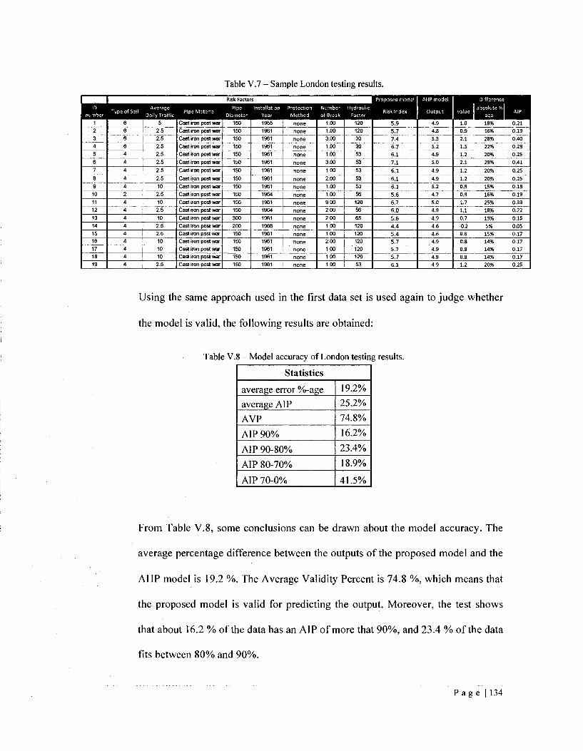
Table V.7 - Sample London testing results.

1

2

3

4

5

6

7

8

9

10

11

12

13

14

15

16

17

18

19

" ~4~" "

4

5

2.5

2.5

2.5

2.5

2.5

2.5

2.5

10

2.5

10 2.5 10

2.5

2.5

10

10

10

2.5

Cast iron post war

Cast iron post war

Cast iron post war

Cast iron post war

Cast iron post war

Cast iron post war

Cast iron post war

Cast iron post war

Cast iron post war

Cast iron post war

Cast iron post war

Cast iron post war

Cast iron post war

Cast iron post war

Cast iron post war

Cast iron post war

Cast iron post war

Cast iron post war

Cast iron post war

150

150

150

150

150

150

150

150

150

150

150

150

300

200

150

150

150

150

150

1955

1961

1961

1961

1961

1961

1961

1981

1981

1964

1961

1964

1981

1988

1961

1961

1961

1961

1981

none

none

none

none

none

none

none

none

none

none

none

none

none

none

none

none

none

none

none

1.00

1.00

3.00

1.00

1.00

3.00

1.00

2.00

1.00

1.00

9.00

2.00

2.00

1.00

1.00

2.00

1.00

1.00

1.00

120

120

30

30

53

53

53

53

53

56

120

56

65

120

120

120

120

120

53

5.9

5.7

7.4

6.7

6.1

7.1

6.1

6.1

6.1

5.6

6.7

6.0

5.6

4.4

5.4

5.7

5.7

5.7

6.1

4.9

4.8

5.3

5.2

4.9

5.0

4.9

4.9

5.2

4.7

5.0

4.9

4.9

4.6

4.6

4.9

4.9

4.9

4.9

1.0

0.9

2.1

1.5

1.2

2.1

1.2

1.2

0.9

0.9

1.7

1.1

0.7

-0.2

0.8

0.8

0.8

0.8

1.2

18%

16%

28%

22%

20%

29%

20%

20%

15%

16%

25%

18%

13%

5%

15%

14%

14%

14%

20%

0.21

0.19

0.40

0.28

0.25

0.41

0.25

0.25

0.18

0.19

0.33

0.22

0.15

0.05

0.17

0.17

0.17

0.17

0.25

Using the same approach used in the first data set is used again to judge whether

the model is valid, the following results are obtained:

Table V.8 - Model accuracy of London testing results.

Statistics

average error %-age

average AIP

AVP

MP 90%

AIP 90-80%

AIP 80-70%

AIP 70-0%

19.2%

25.2%

74.8%

16.2%

23.4%

18.9%

41.5%

From Table V.8, some conclusions can be drawn about the model accuracy. The

average percentage difference between the outputs of the proposed model and the

AHP model is 19.2 %. The Average Validity Percent is 74.8 %, which means that

the proposed model is valid for predicting the output. Moreover, the test shows

that about 16.2 % of the data has an AIP of more that 90%, and 23.4 % of the data

fits between 80% and 90%.

P a g e | 134

Checking the results obtained from the two tests and keeping in mind the points

mentioned earlier about the AHP model, one can say that the model is accurate enough to

be used in the industry. Furthermore, the proposed model is rather recommended to be

used than the AHP model since it considers the uncertainty of the water main parameters,

it considers more risk factors especially post-failure factors (consequences factors) which

are not considered in the AHP model.

V.8. Proposed Risk of Failure Scale

In light of reviewing section II.5. Risk and Condition Rating Scale, a risk of failure scale

is proposed to help the decision makers in water main management

companies/municipalities make an informed decision. The scale ranges numerically from

0 to 10, where 10 indicates the riskiest condition of the pipeline and 0 indicates the least

risky condition. Linguistically, the scale is divided into five groups or regions that

describe the risk of pipeline failure and the required corrective actions to be taken if

needed. The number of proposed groups and their ranges and associated corrective

actions may be changed to best suit a municipality's strategies and their risk tolerance.

P a g e | 135

Figure V.36 - Proposed risk of failure scale.

The advantage of using a scale from 0 to 10 is that it provides an easy way of making

comparisons and conversions to other types of scales such as a scale from 0 to 100 or a

scale from 0 to 5.

V.9. Case Study Application

In this chapter, the developed HFES model will be applied to the collected datasets to

analyze the situation simulating a real management problem. Three data sets are collected

from two municipalities, the City of Moncton and the City of London as explained in

IV.2. Case Study Data Sets.

P a g e | 136

V.9.1. Case Study 1

Data set one is processed using HFES model and the proposed scale. Table V.9 shows a

sample of the results. Table V.10 and Table V.10 summarize the results of the data set

assessment using the proposed HFES model. It can be deduced that Cast Iron and Small

Diameter pipes (< 250 mm) contribute most to network risk. Overall, the condition of the

network is fair (66% of the network) with some parts of the network requiring mitigation

action in the short-term plan as shown in Figure V.37.

Table V.9 - Sample case study 1 results.

i zs ! 8.3 i 7.5 ! 7.3 1 7.3 | 8.3 1 7.8 1 7.7 | 7.6 | 6.9 1 6.8 | S.3 i 7.1 1 7.3 [ 7.6

7.5 | 8.0 1 7.S

6.0 S 3 3.8 4.5 3.2 6.7 3.8 6.7 5.1 3.6

3.1 4.7 5.4 4.0 1.7 3.4 3.3 S.5

6.7 5.1 2.5

1.7 5.1 1.7 6.1 5.1 1.7 1.7 1.7 1.7 2.2 1.7 1.7 1.7 1.7 5.1

7.5 8.3 7.5 7.4 7.4 8.3 7.7 7.6 7.6 7.0 6.9 8.3 7.2 7.4 7.6 7.5 7.9 7.7

5.7

S.7

. 5 '

4.7"

5.6. .S.7"' •

"4.3

5.2 5.0

'[""Hii M i ' iiiiiriiii r "iiin

Table V.10 - Case study 1 results summary.

Linguistic Group

Very Good

Good

Fair

Risky

Very Risky

_ , . . No. of water Proposed Action r main

No action required 15

Watch out 93

Mitigation action in long-term plan 373

Mitigation action in short-term plan 63

Immediate mitigation action required 0

Total : 544

Length, m

4,503

34,462

101,248

12,831

0

153,044

P a g e I 137

Table V.l 1 - Case study 1 pipes statistics of Fair, Risky and Very Risky status.

Pipe Characteristics D

ia.

Mat

eria

l

Small

Medium

Cast Iron

Cast Iron Post War

Asbestos

Ductile Iron

Fair

Count

314

57

56

282

18

15

Length m

73,053

28,196

17,057

73,157

6,578

4,457

Risky

Count

65

1

49

17

0

0

Length m

12,751

80

10,337

2,494

0

0

Very Risky

Count

0

0

0

0

0

0

Length m

0

0

0

0

0

0

Figure V.37 - Water main risk distribution of case study 1.

The results can be further analyzed using the GIS system which provides the opportunity

to locate the different pipes and ease the setup of a management plan. The pipes that are

assessed using the proposed model are shown in Figure V.39. The pipes are colored and

grouped according to their risk of failure score. The groups are the same proposed in the

P a g e | 138

risk of failure scale: Very Good, Good, Fair, Risky, and Very Risky. After reviewing the

pipelines' locations, the management team may decide to renew or rehabilitate the risky

pipelines. However, due to the fact that the risky pipelines are located in an almost

enclosed area, the management team may decide to include the pipelines at fair risk

(which will need mitigation actions in the long-term plan) in the rehabilitation plan to

save on the costs of mobilization and equipment transportation. The management team

may include only the pipes at fair risk that are top ranked or may not include any fair risk

pipes according to the allocated budget. Figure V.40 shows a proposed area to be

included in a rehabilitation plan which includes both risky and fair pipes. The short-term

rehabilitation plan can be set for every year or any other period of time depending on a

management team's preference. It should be noted that not all the risky pipes are included

in the plan since some are remote from the proposed area and they will require a

considerable amount of money to rehabilitate them to account for the cost of mobilization

and transportation, and thus the management team may be willing to carry the risk of

failure by doing nothing to these pipes. Table V.12 shows a sample of the selected pipes

for the short-term rehabilitation plan. Table V.13 summarizes the characteristics of the

selected pipes. Figure V.38 illustrates a framework on how the decision can be taken

regarding water main management using the proposed model.

Table V.12 - Sample selected pipes for short-term rehabilitation plan.

Number

1 2 3 4

5

Pipe Type

Cast Iron

Cast Iron

Cast Iron

Cast Iron

Cast Iron

Year Installation

1920

1895

1907

1896

1895

Diam

254

102

102

102

102

Risk of Failure

6.8 6.7 6.7 6.7 6.7

Risk Group

Risky

Risky

Risky

Risky

Risky

P a g e | 139

Table V.13 - Summaries of the selected pipes for short-term rehabilitation plan.

Pipe Characteristics D

ia.

Mat

eria

l

Small

Medium

Cast Iron

Cast Iron Post War

PVC

Ductile Iron

Fair

Count

37

17

28

23

2

1

Length m

6,996

6,252

8,567

4,075

314

292

Risky

Count

46

0

31

13

2

0

Length m

9,836

0

7,639

1,816

381

0

Very Risky

Count

0

0

0

0

0

0

Length m

0

0

0

0

0

0

\r Collect

information about the water main

network

-\r Assess the water main for Risk of Failure using the developed model

J\.

Locate water main on Geographic

Information System

^V

r \r Divide the map

into regions that need long-term, short-term, and

immediate management

plans

Compare the estimated cost

against the allocated budget

and make the required

adjustments

Figure V.38 - Decision making flow chart.

P a g e | 140

* La

yers

I 0

Risk

y

\ 0

Fair

1 0

Goo

d

1 0

Ver

yjS

ood

; Q

R

ehab

ilitat

ion

Plan

S

D

Fa

ir se

lect

ion

-I

SS D

R

isky

sele

ctio

n

0_

^8jjj

Sa

tfp

6J

SB

fect

pttj

/

F°

*jlL

Figu

re V

.39

- W

ater

mai

n as

sess

ed a

gain

st th

e ri

sk o

f fai

lure

.

Pa

ge

| 141

Figu

re V

.40

- Pr

opos

ed r

ehab

ilita

tion

area

(Ris

ky a

nd F

air

pipe

lines

).

Pa

ge

| 142

V.9.2. Case Study 2

Using the same weights collected from experts and the proposed scale, the data set 2 is

processed using the developed model. Table V.14 shows a sample of the results. Table

V.15 and Table V.16 summarize the results of processing the data set, which show that

the Cast Iron Post War material and Small Diameter pipes contribute most to the risky

situation of the network. Overall, the condition of the network is risky (50%) to fair

(47%) with some parts of the network requiring immediate mitigation action as shown in

Figure V.41.


Environmental Index

7.4

7.3

6.2

6.7

8.S

7.9

5.0

7.4

8.3

6.2

S.7

6.9

S.5

S.S

6.2

7.3

7.8

6.7

5.0

7.4

8.7

7.4

7.4

7.2

Physical Index

6.6

6.6

6.6

7.5

S.3

7.5

7.3

7.3

8.3

7.8

7.7

7.6

6.9

6.8

8.3

7.1

7.3

7.6

7.5

8.0

7.8

7.4

7.4

7.0

Operational Index

4.8

2.8

3.1

5.6

4.8

4 .8

5.0

3.5

5.9

4 .8

7.0

5.7

3.8

S. l

6.5

6.2

4.7

3.3

4.7

3.3

5.7

6.7 — 51

M

Consequence* Index

8.3

6.7

8.5

5.0

4 .1

5.9

7.4

6.7

7.9

3.3

6,7

4 .5

6.7

5.0

8.3

7.4

6.7

7.1

6.7

6.7

8.3

7.2

4 .3

7.4

Prefatiure Index

6 .4

4 .9

4 .9

7.4

6,6

6.3

6.7

5.7

7.6

6.4

7.6

7.4

5.5

6 .8

8.0

7.2

6.2

5.9

6.2

6.2

7.4

7.4

6.9

5.4

P a g e | 143

Table V.15 - Case study 2 results summary.

Linguistic Group

Very Good

Good

Fair

Risky

Very Risky

Proposed Action

No action required

Watch out

Mitigation action in long-term plan

Mitigation action in short-term plan

Immediate mitigation action required

Total

No. of water main

0

3

210

310

21

: 544

Length, m

0

512

72,293

75,535

4,704

153,044

Table V.16 - Case study 2 pipes statistics of Fair, Risky and Very Risky status.

Pipe Characteristics

Dia

. M

ater

ial

Small

Medium

Cast Iron

Cast Iron Post War

PVC

Asbestos

Ductile Iron

Fair

Count

164

46

16

87

9

9

89

Length m

41,697

30,596

5,114

26,179

2,511

4,167

34,322

Risky

Count

277

33

80

211

1

9

9

Length m

61,389

14,186

20,841

50,669

87

2,411

1,527

Very Risky

Count

21

0

10

11

0

0

0

Length m

4,704

0

2,069

2,635

0

0

0


P a g e | 144

V.9.3. Case Study 3

Using the same weights collected from experts and the proposed scale, the data set is

processed using the developed model. Table V.17 shows a sample of the results. Table

V.18 and Table V.19 summarize the results of the data set assessment using the proposed

fuzzy model. The overall condition of the network is fair (50%) to risky (45%) with some

parts of the network requiring immediate mitigation action as shown in Figure V.42.


Environmentaljndex

6.4

5.7

5.7

5.7

3.6

3.6

3.6

3.6

5.2

1.5

5.2

3.6

5.2

3.6

3.6

5.2

5.2

5.2

3.6

PhysicaMndex

7.7

7.3

7.3

7.3

7.3

7.3

7.3

7.3

7.3

7.1

7.3

7.1

6.3

6.1

7.3

7.3

7.3

7.3

7.3

Operationa!_lndex

3.3

3.3

7.6

6.7

6.3

7.3

6.3

6.3

6.3

6.1

6.7

6.1

5.5

3.3

3.3

3.3

3.3

3.3

6.3

Consequencejndex

5.0

1.7

1.7

5.0

1.7

1.7

1.7

5.0

1.7

5.0

1.7

1.7

7.3

6.1

5.0

5.0

5.0

5.0

1.7

Prefailurejnde X

5.9

5.7

7.4

6.7

6.1

7.1

6.1

6.1

6.1

5.6

6.7

6.0

5.6

4.4

5.4

5.7

5.7

5.7

6.1

Risk of Failure Index

5.7 "57"

5 7 5.7 5 / S6~ 5 7 S6

5.0 sT4" 57" 5.7 5.7" 5 7

Linguistic Group

Very Good

Good

Fair

Risky

Very Risky

Table V.l 8 - Case study 3 results summary.

Proposed Action

No action required

Watch out

Mitigation action in long-term plan

Mitigation action in short-term plan

Immediate mitigation action required

Total :

of water main

2

58

823

798

21

1702

Length, m

245

11,118

137,453

123,136

2,823

274,773

P a g e I 145

Table V.19 - Case study 3 pipes statistics of Fair, Risky and Very Risky status.

rj r ipe v^iiaiavAciisucs

Dia

. M

ater

ial

Small

Medium

Cast Iron

Cast Iron Post War

PVC

Concrete

Ductile Iron

Fair

Count

729

94

61

636

4

1

121

Length m

120,265

17,189

10,888

109,265

298

171

16,832

Risky

Count

730

68

322

475

0

0

1

Length m

111,285

11,850

43,492

79,300

0

0

344

Very Risky

Count

21

0

14

7

0

0

0

Length m

2,823

0

1,643

1,180

0

0

0


To further analyze the outputs, the dataset's records are clustered according to pipe

material (Cast Iron, Cast Iron post war, Ductile Iron, and PVC) and according to their

scores (10 groups). Table V.20 and Figure V.43 show the percentages scores of each

material (local percentages for each material are not comparable to other materials). It

can be deduced that the majority score of the Cast Iron material falls in the range between

P a g e | 146

6 and 7. However, for Cast Iron Post War pipes, the scores form a triangular shape

between 3 and 8 with a peak between 5 to 6 that has 48.66 % of the cast iron post war

material. Ductile Iron material pipes also form a triangular shape from 2 to 7, with a peak

between 4 and 5 with 63.86 % of the Ductile Iron material pipes. Figure V.44 shows the

pipe material global scores percentages. It can be concluded that the Cast Iron Post War

material contributes in large part to the fair-risky status of the London water main

network, as 55% of that network is Cast Iron Post War with scores between 5 and 7.

Table V.20 - Pipes material percentage score.

Cast Iron Cast iron post war Ductile iron PVC

• Otol ml to 2 • 2 to 3 • 3 to 4 • 4 to 5 a 5 to 6 • 6 to 7 w 7 to 8 li 8 to 9 • 9 to 10

Figure V.43 - Pipes material local score percentage.

P a g e | 147

Figure V.44 - Pipes material global score percentage.

V.10. Summary

This chapter presented the work done in building the FHES model. It explains into details

the different stages in the model building, starting from the considered factors and their

linguistic membership functions, through the fuzzy rules extraction and evaluation

process, the rules aggregation and the deffuzification process. The sensitivity of the

FHES model is tested and analyzed and the results showed that the model is robust and

sound. The FHES model is also verified using a validated AHP model. It also showed the

proposed failure risk scale. Three case studied are evaluated and studied using the

developed model in order to show the probable use of the model in the field of water

main management.

P a g e | 148

Chapter VI: EXCEL-BASED APPLICATION

DEVELOPMENT

VI.l. Introduction

An application was developed to implement the designed model. This

application is based on MS© Excel 2007 and thus requires this program in order

to run. Excel 2007 was chosen over earlier Excel versions because of the

extended size of the worksheet which is required to handle all the fuzzy expert

system calculations, where the earlier versions cannot handle. In addition, Excel

2007 has more options, functions, and visual aids and it results in a compressed

smaller file size and a lighter load on computers.

VI.2. Working Folder and Files

The working folder which contains the files is named as "Risk of Water Main

Failure". This folder can be saved any where on the computer hard disk and the

links between different excel files will still be functioning. The folder contains

nine Excel files and these files are explained as follows:

- Navigation: this file contains all the step-by-step instructions which will

guide the user to an easy use of the application. Moreover, it allows the

P a g e | 149

user to easily fine tune the factors weights and the expert knowledge base.

The file contains two worksheets "Control Panel" and "Fine Tune".

"Control Panel" worksheet guides the user to setup the application and

enter the required information to run the model. It starts with "Important

Notice" on how to deal with security issues and how to enable the macros

which are needed to run the application as shown in Figure VI. 1 (a).

Then, the worksheet contains three steps which will setup and run the

application. The first step is "Step 1 - Prepare the Data" (Figure VI. 1 (b))

which has a link to another excel file that stores the information about the

different performance characteristics on the water main network. This file

is named "Network Performance Data" and will be explained hereafter.

The next step is "Step 2 - Prepare the Model" which controls the factors weights

and even allows the user to save the weights according to his own preferences

giving the user the full flexibility as shown in Figure VI. 1 (c). Moreover, the user

can choose the factors to be incorporated in the risk assessment.

(a)

P a g e | 150

Prepare your Data

(b)

"K&tf 7 ;^'^9t^^,*^

iiMai Fine ~uric? tho Model

(c)

Stop 3 - Run t h e M o d r l & S h o w t h e ResuVts

Run the Mode!

View the Results

Copy the Results to a New File

(d)

Figure VI. 1 - Control panel worksheet in Navigation workbook.

P a g e |

In addition to that, this panel contains a button that links to the other worksheet

"Fine Tune", which enables the user to change the expert knowledge base to best

suit the user own experience and preferences. Figure VI.2 shows how to tune the

Environmental Factors knowledge base.

Environmental Factors •iiOTiHaro.nnnamiaBiimftniiiHinBHm.Hrornai

if soil is Very lightly deteriorative if soil is Lightly deteriorative if soil is Moderately deteriorative if soil is Highly deteriorative if soil is Very highly deteriorative

if ADT is Very light if ADT is Light if ADT is Moderate if ADT is Heavy if ADT is Very heavy

3. What is

then the risk of failure is then the risk of failure is then the risk of failure is then the risk of failure is then the risk of failure is

then the risk of failure is then the risk of failure is then the risk of failure is then the risk of failure is then the risk of failure is

Extremely Low Very Low Medium Very High Extremely High

Extremely Low Very Low Medium Very High Extremely High

if WTL is rarely present if WTL is seasonally present if WTL is always present

HI

the risk of failure is the risk of failure is the risk of failure is

Extremely Low Extremely High Moderately High

Figure VI.2 - Fine tuning of the environmental factors attributes.

The third and last step is "Step 3 - Run the Model & Show the Results",

which contains "Run the Model" button that opens the six other excel

files one by one, and runs the macros to perform the required calculations.

These files, which are explained later in this section, are: "Environmental

Factors", "Physical Factors", "Operational Factors", "Post Failure

Factors", "Pre-failure Model", and "Risk of Failure Model". The "View

the Results" button opens the "Results" file and shows the calculated risk

of failure for each record stored in "Network Performance Data". The

"Copy the Results to a New File" button copies the risk of failure results

P a g e | 152

stored temporary in the "Results" Excel file to a new file that will store

the results permanently as shown in Figure VI. 1 (d).

- Network Performance Data: This Excel file stores the attributes and

performance characteristics of the water distribution network. It contains

seventeen columns which correspond to the sixteen risk factors (Loss of

production factor requires two columns: pipe diameter and redundancy).

The total number of records which can be stored in this excel file is

limited to 2000 records due to huge computer resource needed to process

the large amount of data. Each of these columns has its own validation

rule which will guide and restrict the user to the type and range of

information to be input into the model. There are four more columns

which can be used to store some notes about each record.

- Environmental Factors, Physical Factors, Operational Factors, and Post

Failure Factors Modules: These Excel files are considered the highest

level in the hierarchy shown in Figure V.2. Their files structures are

similar, and thus for illustration purposes, only the "Environmental

Factors" Excel file structure will be explained here. This Excel file

contains two worksheets: "Environmental Model" and "Enviro Process".

The "Environmental Model" worksheet contains all the calculations

required to generate the dynamic rules. The weights of the factors and the

expert knowledge base are directly linked to the "Navigation" Excel file

P a g e | 153

and thus any changes made to "Navigation" will be directly reflected in

this worksheet. This worksheet consists of two parts; part one contains the

different environmental factors, their associated antecedents, membership

functions and their consequents. The second part contains all the possible

rules that are constructed and shown in Section IV.1.3. Expert knowledge

base. The other worksheet, "Enivro Process", contains all the calculations

required to process the data available about the network attributes and

performance characteristics as stored in "Network Performance Data"

file and to generate the estimated index for each record in the data. This

worksheet contains many sections. It starts with fuzzification of the real

data (stored in the "Network Performance Data" Excel file) in which the

real network data is used to generate membership values for the

membership functions of the different factors as shown in Figure VI.3 (a).

The upper part of the table shows the membership functions of the factors

as stored in the first worksheet "Environmental Model" which will be

used to fuzzify the real data records. The results of fuzzification of the

real data are shown underneath the membership functions which are

identified by records serial numbers. The assessment of two records is

shown in Figure VI.3.

P a g e | 154

s H n tm

1 1 3 1 • :

1

1 -I > 1 I ? .

1 ..... J » ! 1 i

1

I > n

•5 .

2 5

2 5

S

2

£ *=i

I . pAp*

£ -= 3

2 5 •

5

5

7 5

*

;

I :

1 -£ 1

5

7.5

7 5

:o 4

* i i j =

i

7.5

:.c iS

10

5

•:. • n J S

S T ? • -E =

: 5

2 5 5

2 5 5

:=> 5 7 5

: 2

Fuaff iotfcmofl leal lMi

2 -

5

7 5

; 5

13

-

e

.z z* £

t'apn»f

7 5 • • • *

10

l j

5

i «.

CS5

--& * S a £

b.&oe-e

CS5

2

I * *

d sc-rte

0 35

3

Water Table Level

(a)

Moderate

Heavy

Very heavy

10

(b)

1 • n i a %

KflMgjl s •JHHgll .» RMH BSI.. M M H " 6

"•

i

1 i 1 : 5

* a

f *

|

5

; . 5 i

: 5

• •

i

« i

i ; I

<

s 4

3

6

S 4

2

S

• "

! «

i ;

i i

1 i s

1 < : i

.J_. ._i .

; « ,1

j

i

S 3

3

S

•^

5 5 2

s

1

- 5 \ 3

* 1

t *

i

!

;

i

; V 1

s » s

5

5 2 2

- 4

0.*

! 1 t

I 1 i 1

! 1 • 5 : r ; .?: i ; • i ;

.T-a . i « i

0.33333

5 1

S

_s

• •

- 5 • 1

2 I

4

0.6

j !

!

s 1 1

1

.*_.. _ J i 3

0,33333

(c)

P a g e | 155

• 1

• B a S H trapmf

1G&9 167

H R I 1

5 a _ j > •

V

>

trapmf

1 6 7

1 6 7

3 33

2

5

> •

it

T>

1 trapini

1G7

3.33

i 3 33

: 5

3

E

"•5

5

trapmf

3 33

5

5

1 6 67

4

±

n u

-a 5

trapm! ;

5

: 6 67 •'

6 67 '

• 8 33 :

5

x; W

>->

trapmf !

6 67

8.33 :

8 33 :

10 :

6

x:

X j j r u C

i U

traomf

8 33

10

10

10

7

Membership value

0.2 0.66661

0.33333 Q.6

>f ou tpy t MF

(d)

1

2

1.6?

2-6?

2.002 2.223S3

4.666

4.44333

5

5

3.33 333

4.44S3S

4.332

5.55667

5.668

6.67

6.6?

(e)

Extremely Low

Very Low

Moderately Low

Medium

Moderately High

Very High

Extremely High

Environmental Index

(g)

Figure VI.3 - Data processing in the excel-based application.

P a g e | 156

Figure VI.3 (b) shows the membership functions of the Average Daily

Traffic factor of the second record of the real data. Its results in a 0.6

membership value for Very light membership function and a 0.4

membership value for Light membership function. This visual aid is also

included in the Excel file.

The next step is to evaluate each rule in the knowledge base. When a rule is

triggered, the minimum (And operation) membership value of the considered

factors from the fuzzification step is calculated and stored for later use in the

aggregation process. Figure VI.3 (c) shows the different rules and the results of

the triggered rules for the second record of the real data.

After assessing all of the triggered rules, the next step is to aggregate the

membership values that resulted from last step according to the membership

function output, and then to choose the maximum membership value (aggregation

method is Maximum) for each linguistic membership function to be used in the

next step, as shown in Figure VI.3 (d). It is worth mentioning that this is the same

approach used in Matlab © software.

The next step is to use these aggregated membership values to truncate

the output membership functions and construct new membership

functions that use the Center of Sum defuzzification method to get an

Environmental Index for each record in the data set. Figure VI.3 (e)

shows the new membership function parameters resulting from the

truncation of the original output membership functions.

P a g e | 157

The calculation of the defuzzification method and the resulting

Environmental Index are shown in Figure VI.3 (f).

A visual aid (chart) is included in the Excel file to best present the

calculation results, as shown in Figure VI.3 (g), where the output

membership functions are truncated and new membership functions are

generated accordingly. This figure also shows the Environmental Index of

the second record calculated using the Center of Sum defuzzification

method.

It should be observed that these four Excel files are read-only and are not

to be altered. Also, it is advisable to check these files only to overview the

calculations or to see the visual aids.

- Risk of Failure Module: The structure of this Excel file is similar to that

of the "Environmental Factors" Excel file. This file is responsible for

combining the results of the four main failure risk factors modules to get

a crisp value of failure risk for a water main. The hierarchy is shown in

Figure V.2. The partial risk indices (environmental index, physical index,

operational index, and post-failure index) are processed as data inputs

instead of the real data used in the second level of the hierarchy.

P a g e | 158

Prefailure Module: This Excel file is a duplicate of the "Risk of Failure"

Excel file. However, it uses only three instead of four inputs:

Environmental index, Physical index, and Operational index. A post-

failure index is precluded in this Excel file. The reason for creating such a

file is to give an idea about the possibility of a failure event in the

pipelines as a prefailure index as opposed to a post-failure index, as

generated before. The hierarchy of the "Pre-failure Model" is shown in

Figure V.3.

- Results: This is the last Excel file in the working folder. It displays all the

indices generated in the six Excel files (Figure VI.4).

ID number Environmental Index

• _*A » . : , " 4.5

4.1 i g n r KS&M . -;* 5.0 S'S.o

Figure VI.4 - The results of the application data processing.

VI.3. Testing of the developed Application's Programming

The objective of this section is to test the internal calculations, procedures and

programming inside the Excel-based application using Matlab ® software. The results

obtained from the developed HFES are compared against the results obtained using

Matlab ©. The tested calculations are the fuzzification process, the rules triggering

process, the fuzzy operations, and the defuzzification process. Two scenarios are

followed to accomplish this, as explained below:

P a g e | 159

1. Using the operational model, the effects of each factor are increased one at a time

from the best performance to the worst performance as shown in Table VI. 1.

2. Using a risk of failure model, maximum and minimum scenarios together with

eight randomly chosen values are examined as shown in Table VI.2.

By analyzing Table VI. 1 and Table VI.2, one can note that the difference between the

results obtained from the developed application and the Matlab ® are very small and

minor, and is due to the different defuzzification methods (Matlab uses the Centriod

method). Also, it can be concluded that even though the Center of Sum defuzzification

method requires far less calculations, it generates fairly precise results.

Table VI. 1 - Operational model Matlab testing.

1

2

3

4

5

6

7

8

9

10

11

12

13

14

15

Operational Model Matlab

Testing

Breakage rate 1

Breakage rate 2

Breakage rate 3

Water Quality 1

Water Quality 2

Water Quality 3

Water Quality 4

Hydraulic Factor 1

Hydraulic Factor 2

Hydraulic Factor 3

Hydraulic Factor 4

Leakage 1

Leakage 2

Leakage 3

Leakage 4

Operational

o • - jat 01 <o

JQ <D

M z

0

2

6

6

6

6

6

6

6

6

6

6

6

6

6

1 o E tS •o m > u-X

130

130

130

130

130

130

130

90

70

50

20

20

20

20

20

>•

3

a 4-* re

5 0

0

0

2.5

5

7.5

10

10

10

10

10

10

10

10

10

0) 00 ra re 2

0

0

0

0

0

0

0

0

0

0

0

2.5

5

7.5

10

Results

-0

JS

1

0.52

1.67

5.00

5.00

5.00

6.67

6.67

6.67

8.33

8.33

8.33

8.33

8.33

9.48

9.48

•D 01 c

a E 0 0{ 01 >»>

> > a

0.60

1.70

5.00

5.00

5.00

6.70

6.70

6.70

8.30

8.30

8.30

8.30

8.30

9.40

9.40

01 u c

2!

'•a

0.08

0.03

0

0

0

0.03

0.03

0.03

-0.03

-0.03

-0.03

-0.03

-0.03

-0.08

-0.08

P a g e | 160

Table VI.2 - Risk of failure model Matlab testing.

1 2 3 4 5 6 7 8 9 10

Risk of Failure Model Matlab Testing

Maximum Minimum random 1 random 2 random 3 random 4 random 5 random 6 random 7 random 8

Risk of Failure

c 01 E c o i . '5 c IU

9.44 0.56 0.56 0.56 1.67 3.33 5.00 8.33 8.33 9.44

re u 'vi > .c a.

8.33 1.67 3.33 5.00 8.33 8.33 8.33 8.33 8.33 8.33

re c _o '** re o> a O

9.44 0.56 0.56 0.56 5.00 5.00 5.00 6.67 8.33 9.44

0) u c ai 3 o-01 c o U

9.44 1.67 1.67 1.67 1.67 1.67 1.67 5.00 5.00 8.33

Results

_re

re

2

8.73 1.67 1.67 2.28 5.00 5.00 5.00 6.67 8.33 8.33

•a v c a c O IU

ai «

a 8.81 1.66 1.67 2.31 5.00 5.01 5.01 6.67 8.33 8.34

o c

1 0.08 -0.01 0.00 0.03 0.00 0.01 0.01 0.00 0.00 0.01

VI.4. Summary

An Excel-based water main failure risk assessment is developed based on the proposed

hierarchical fuzzy expert system of water main risk of failure model. The model

calculations and data flow is checked using Matlab software and the results show that the

developed application passes the test are ready to be used. This application can be used

by municipal and consultant engineers to estimate the failure risk associated with water

mains in order to better manage their distribution network and spend the allocated budget

more efficiently.

P a g e | 161

Chapter VII: CONCLUSIONS AND RECOMMENDATIONS

VII.l. Summary

This work has presented a methodology that addresses the challenge faced by

municipalities and other authorities of prioritizing the rehabilitation of water main

systems. It offers a model to evaluate the risk of water main failure that considers many

risk factors, which can be divided broadly into deterioration factors that lead to the failure

event and consequence factors that result from a failure event (failure impact). Sixteen

failure risk factors are incorporated in the model (11 deterioration factors and 5

consequence factors). A hierarchical fuzzy expert system (HFES), which takes into

account the uncertainty in the water main attributes, is used to build this model. The use

of hierarchy allows the number of knowledge base rules required to construct the model

to be reduced. The model is verified using a validated AHP deterioration model and two

different data sets (from the cities of Moncton, NB and London, ON). A water main

failure risk scale is proposed, which ranges numerically from 0 to 10 where 0 indicates

the lowest risk situation and 10 the highest risk situation. Linguistically, the scale is

divided into five zones: "Very good, Good, Fair, Risky, and Very Risky". Each of these

zones proposes appropriate actions to mitigate the risk, as appropriate. Three case studies,

from different potable water networks, are assessed using the developed model. The

P a g e | 162

results of risk assessment of these case studies are analyzed and rehabilitation plans are

proposed accordingly.

Based on the developed model and the proposed failure risk scale, an Excel®-based

application is developed to assess and evaluate the risk of failure associated with the

water main and advises the management team of some proposed mitigating actions.

Municipal water main managers, consultants, and contractors can use the developed

application to assess the risk of water main failure and to plan their rehabilitation works

accordingly. The application provides a high level of flexibility to adapt to management

preferences and the outlook of each authority.

VII.2. Conclusions

This research offers a HFES model to assess the risk of failure of water mains. During the

course of the research, many points can be noticed and concluded such as:

• HFES model is recommended to assess the risk of failure associated with water

main since it can deal with the vague and uncertain characteristics (factors) of the

water main.

• From the collected questionnaire, it can be deduced that pipe age has the highest

effect on risk of water main failure (100 units of global weight), followed by pipe

material (75 units) and breakage rate (57 units).

• The more the data collected about the water main is, the more the HFES results

accuracy is. However, it is so advisory to keep records and collect data about the

P a g e | 163

most important factors (most weighted) (i.e. Pipe age, material, breakage rate).

This will result in more reliable management plans.

• The model is more sensitive toward the most weighted factors (i.e. pipe age, pipe

material, and breakage rate).

• Due to the rules evaluation and aggregation, and to the defuzzification process,

the model tends to produce results at some certain numbers and will not be

distributed in a smooth curve, which is undesirable.

• It is difficult to make a change in the Risk of Failure value by only changing the

performance of one factor, since the other fifteen factors try to resist the change in

the risk values.

• Each of the four main branches of the hierarchy (environmental, physical,

operational, and post failure) is sensitive to their own factors more than the risk of

failure model is. This fact is due to the use of a hierarchical system where the

farther the factor is in the hierarchy, the less its effectiveness (sensitivity) is.

• It can be deduced that the model is not very sensitive to the weight of the factors

when changed within the factors' standard deviations.

• The Average Validity Percent of the model is 74.8 %, which means that the

proposed model is valid for predicting the output. Moreover, the test shows that

about 16.2 % of the data has an Average Invalidity Percent of more that 90%, and

23.4 % of the data fits between 80% and 90%.

P a g e | 164

VII.3. Research Contributions

The developed fuzzy expert model solved the problem of assessing the risk of failure

associated with water mains. It contributes to the state of the art of sustainably managing

water main infrastructure by achieving the following:

• A water main failure risk model.

• An automated tool (Excel-based application) that helps water main network

managers build their short-term management plans and estimate their

requirements for long-term plans.

• A failure risk scale that will provide guidance to decision makers to make the

best-informed decisions.

VII.4. Limitations

VII.4.1. Model Limitations

The developed model uses hierarchical fuzzy expert system technique to assess the water

main risk of failure. There are some limitations inherent in the model such as:

• The number of collected questionnaires is twenty. The model accuracy can be

improved by increasing the number of experts involved in building the knowledge

base rules of the fuzzy expert system.

• The model considers only eleven factors that indicate or contribute to the failure

event and five factors that represent failure consequences.

P a g e | 165

• The input data membership functions in the model are limited to triangular and

trapezoidal.

• A 95% confidence level is assumed as membership constant value for all of the

linguistic input factors (i.e. pipe material, protection method, business

disruption,...).

• The number of output membership functions (risk of failure membership

functions) is limited to seven. Increasing this number will increase the accuracy of

the model.

• The proposed risk of failure scale only gives some recommendation on how to

manage the water mains at different risk stages. However, it is not built on a

sound bases and can be improved in the future work.

VII.4.2. Application Limitations

An Excel-based application was built based on the developed model which uses

hierarchical fuzzy expert system. However, there are some limitations to using this

application:

• Even though the application leaves a flexible space for the user to choose among

the sixteen considered factors, some other factors may come into the play, which

are not considered in this model.

• Expert systems are built on expert opinions and thus the knowledge database

represents the consensus among the experts ~ however, some users may prefer to

consider other opinions (e.g. to adapt for hot or cold climate or specific local

P a g e | 166

conditions). The flexibility to modify the knowledge database is therefore

provided in the application which on the other hand causes the sensitivity analysis

conducted in this research to be invalid.

• Due to technical restraints (computer resources), the input membership functions

are limited to a maximum of five and the output membership functions are limited

to seven.

• The developed application is based on MS Excel® version 2007, and thus it

requires this software to operate and function.

VII.5. Recommendations and Future Works

Some of the recommendation and future works that can enhance the model and the

research in general are listed below:

VII.5.1. Research Enhancement

The developed model can be enhanced by:

• More factors can be considered in the model; environmental, physical, operational

factors and especially the consequence of failure factors.

• Some of the qualitative factors can be quantified. However, this step requires

more effort to study in more details the different aspects of each factor.

• The consequences of failure factors may require more research since they have

not conceived enough attention or understanding in the industry field and in the

common practice.

P a g e | 167

• A detailed risk of failure scale and the associated corrective actions can be built

that best utilize the results of the model to establish water main rehabilitation

plans.

VII.5.2. Research Extension

Future efforts on this research could:

• Consider a third level of the hierarchy. This will lead to a better understanding

and evaluation of the risk factors of the second level of the hierarchy (the sixteen

risk factors considered in this research). As a result, the accuracy of the model

output will be improved.

• Incorporate Geographic Information System in the research as the rehabilitation

plans can also consider grouping water mains that are in the same area in order to

more efficiently use allocated budgets.

• Adapt the HFES model to assess the risk of failure of different underground

infrastructure such as transmission water main and sewer main.

Page | 168

Chapter VIII: REFERENCES

Al Barqawi, H. (2006). "Condition Rating Models for Underground Infrastructure:

Sustainable Water-Mains." MS Thesis, Concordia University, Montreal, QC.

Bandyopadhyay, T., Dey, P., and Gupta, S. (1997). "A cost-effective maintenance

program through risk analysis." AACE International Transactions, AACE, Dallas, TX,

84-89.

Bhave, P. (2003). Optimal Design of Water Distribution Networks. Alpha Science Int'l

Ltd., Oxford.

Bogardi, I., and Duckstein, L. (2002). "The Fuzzy Logic Paradigm of Risk Analysis."

Risk-Based Decisionmaking in Water Resources, ASCE, Santa Barbara, CA, 12-22.

Christodoulou, S., Aslani, P., and Vanrenterghem, A. (2003). "Risk Analysis Framework

for Evaluating Structural Degradation of Water Mains in Urban Settings Using

Neurofuzzy Systems and Statistical Modeling Techniques." World Water and

Environmental Resources Congress, ASCE, Philadelphia, PA, 1-9.

Chughtai, F. (2007). "An Integrated Approach to Sewer Pipeline Condition Assessment."

MS Thesis, Concordia University, Montreal, QC, Canada.

Cooke, R., and Goossens, L. (2004). "Expert judgement elicitation for risk assessments of

critical infrastructures." Journal of Risk Research, 7(6), 643-656.

P a g e | 169

Cromwell, J., Reynolds, H., Pearson, N., and Grant, M. (2002). Costs of Infastructure

Failure, Awwa Reseach Foundation and American Water Works Association,

Washington DC.

Del Campo, E. (2004). "Design of Fuzzy Systems Using Knowledge Extracted Via

Neural Networks." MS Thesis, University of Texas, El Paso, TX.

Dillon Consulting, L., and harfan Technologies, I. (2003). Watermain Transmission and

Distribution System Needs Assessment Study, City of Moncton, Moncton.

Ezell, B., Farr, J., and Wiese, 1. (2000). "Infrastructure Risk Analysis Model." Journal of

Infrastructure Systems, 6(3), 114-117.

Gentile, M. (2004). "Development of a Hierarchical Fuzzy Model for the Evaluation of

Inherent Safety." PhD Dissertation, Texas A&M University, Texas.

Giustolisi, O., Laucelli, D., and Savic, D. (2006). "Development of rehabilitation plans

for water mains replacement considering risk and cost-benefit assessment." Civil

Engineering and Environmental Systems, 23(3), 175-190.

Hahn, M., Palmer, R., and Merr, M. S. (2002). "Expert System for Prioritizing the

Inspection of Sewers:Knowledge Base Formulation and Evaluation." Journal of Water

Resources Planning and Management, 12 8(2), 121 -129.

Haimes, Y. (2004). Risk Modeling, Assessment, and Management, 2nd ed., Wiley-IEEE,

Hobocen, New Jersey.

Huanga, C , and Moraga, C. (2005). "Extracting fuzzy if-then rules by using the

information matrix technique." Journal of Computer and System Sciences, 70, 26-52.

InfraGuide, N. G. (2003, April). "Deterioration and Inspection of Water Distribution

Systems." A Best Practice by the National Guide to Sustainable Municipal

P a g e | 170

Infrastructure, <http://www.infraguide.ca/bestPractices/default_e.asp> (Jan. 14,

2007).

InfraGuide, N. G. (2006, July). "Managing Risk." Decision Making and Investment

Planning, <http://www.infraguide.ca/bestPractices/PublishedBP_e.asp#dmip> (Jan.

17,2007).

Infrastructure Report (2007). "The Water Main Break Clock" Canada Free Press,

<http://www.canadafreepress.com/infrastructure.htm> (Jan. 23, 2008).

Jin, Y. (2003). Advanced Fuzzy Systems Design and Applications. A Springer-Verlag

Company, New York.

Karray, F., and de Silva, C. (2004). Soft Computing and Intelligent Systems Design.

Pearson Education Limited Essex, England.

Kirchhoff, D., and Doberstein, B. (2006). "Pipeline risk assessment and risk acceptance

criteria in the State of Sao Paulo, Brazil." Impact Assessment and Project Appraisal,

24(3), 221-234.

Kleiner, Y., and Rajani, B. (2000). "Considering Time-dependent Factors in the

Statistical Prediction of Water Main Breaks." A WW A Infrastructure Conference,

Baltimore, MD, 1-12.

Kleiner, Y., and Rajani, B. (2002). "Forecasting Variations and Trends in Water-Main

Breaks." Journal of Infrastructure Systems, 8(4), 122-131.

Kleiner, Y., Sadiq, R., and Rajani, B. (2004). "Modeling Failure Risk in Buried Pipes

Using Fuzzy Markov Deterioration Process." Pipeline Engineering and Construction:

What's on the Horizon?, ASCE, San Diego, CA, 1-12.

P a g e | 171

http://www.infraguide.ca/bestPractices/default_e.asp

http://www.infraguide.ca/bestPractices/PublishedBP_e.asp%23dmip

http://www.canadafreepress.com/infrastructure.htm

Kleiner, Y., Rajani, B., and Sadiq, R. (2006). "Failure risk management of buried

infrastructure using fuzzy-based techniques." Journal of Water Supply Research and

Technology : Aqua, 55(2), 81-94.

Lee, M. (2006). "Risk Assessment of Drinking Water supply in Cananda." MS Thesis,

University of Guelph, Ontario.

Lee, M.-L., Chung, H.-Y., and Yu, F.-M. (2003). "Modeling ofhierarchical fuzzy

systems." Fuzzy Sets and Systems, 138(2), 343-361.

Marshall, D., Zarghamee, M., Mergalas, B., and Kleiner, Y. (2005). "Tarrant Regional

Water District's Risk Management Plan for Prestressed Concrete Cylinder Pipe." The

Pipeline Division Specialty Conference, ASCE, Houston, TX, 854-861.

Moglia, M., Burn, S., and Meddings, S. (2006). "Decision support system for water

pipeline renewal prioritisation." ITcon, 11 (Special Issue Decision Support Systems

for Infrastructure Management), 237-256.

Mohitpour, M., Golshan, H., and Murray, A. (2003). Pipeline Design and Construction:

A practical Approach, 2nd ed., ASME Press, New York.

Muhlbauer, W. K. (2004). Pipeline Risk Management Manual, 3rd ed., Gulf Professional

Publishing, Burlington.

Najafi, M. (2005). Trenchless Technology: Pipeline and Utility Design, Construction,

andRenewa,. The McGraw-Hill Companies, New York.

Najjaran, H., Sadiq, R., and Rajani, B. (2004). "Modeling pipe deterioration using soil

properties - An application of fuzzy logic expert system." Pipeline Engineering and

Construction: What's on the Horizon?, ASCE, San Diego, CA, 1-10.

P a g e | 172

Nasiri, F., Maqsood, I., Huang, G., and Fuller, N. (2007). "Water Quality Index: A Fuzzy

River-Pollution Decision Support Expert System." Journal of Water Resourses

Planning and Management, 133(2), 95-105.

Nikolaidis, E., Ghiocel, D., and Singha, S. (2005). Engineering design reliability

handbook, CRC Press, Florida.

Oppenheimer, P. (2004). Top-Down Network Design, 2nd ed., Cisco Press, New York.

Ozger, S. S. (2003). "A semi-pressure-driven approach to reliability assessment of water

distribution networks." PhD Dissertation, Arizona State University, Arizona.

Pelletier, G., Mailhot, A., and Villeneuve, J.-P. (2003). "Modeling Water Pipe Breaks-

Three Case Studies." Journal of Water Resources Planning and Management 10,

129(2), 115-123.

Pickard, M. (2007). "The Economics of Pipeline Repair" Clock Spring Company, L.P.,

<www.clockspring.com/quarterly%2520072006/The%2520Economics%2520of%252

0Pipeline%2520Repair.pdf+cost+repair+of+pipelineandhl=enandct=clnkandcd=3>

(May 15,2007).

Rahman, S. M. (2007). "Condition Assessment Tool For Elements of Drinking Water

Treatment Plant." MS Thesis, Concordia University, Montreal, QC.

Rajani, B., Kleiner, Y., and Sadiq, R. (2006). "Translation of pipe inspection results into

condition ratings using the fuzzy synthetic evaluation technique." Journal of Water

Supply Research and Technology: Aqua, 55(1), 11 -24.

Raven, A. (2007). "Risk Factors of Structural Degradation of an Urban Water

Distribution System." Journal of Infrastructure Systems, 13(1), 55-64.

P a g e | 173

http://www.clockspring.com/quarterly%2520072006/The%2520Economics%2520of%252

Rogers, P. (2006). "Failure Assessment Model to Prioritize Pipe Replacement in Water

Utility Asset Management." Phd Dissertation, Colorado State University, Colorado.

Sadiq, R., Rajani, B., and Kleiner, Y. (2004). "Probabilistic risk analysis of corrosion

associated failures in cast iron water mains." Reliability Engineering and System

Safety, 86(\), 1-10.

Santosh, Vinod, G., Shrivastava, O., Saraf, R., Ghosh, A., and Kushwaha, H. (2006).

"Reliability analysis of pipelines carrying H2S for risk based inspection of heavy

water plant." Reliability Engineering and System Safety ,91,163-170.

Selvakumar, A., Clark, R., and Sivaganesan, M. (2002). Costs for Water Supply

Distribution System Rehabilitation. Environmental Protection Agency, New Jersy.

Shaheen, A. A. (2005). "A Framework for Integrating Fuzzy Set Theory and Discrete

Event Simulation in Construction Engineering." PhD Dissertation, University of

Alberta, Edmonton.

Shi, Y., and Sen, P. (2000). "A New Defuzzification Method for Fuzzy Control of Power

Converters." IEEE, 2(9), 1202-1209.

Shi, Y., Mizumoto, M., and Shi, P. (2002). "Fuzzy IF-THEN Rule Generation Based on

NeuralL Network and Clustering Algorithm Techniques." TENCON '02. Proceedings,

IEEE, Beijing, China, 651-654.

Skipworth, P., Cashman, A., Engelhardt, M., Saul, A., and Savic, D. (2001).

"Quantification of Mains Failure Behavior in a Whole Life Costing Approach to

Distribution System Management." World Water and Environmental Resources

Congress 2001, ASCE, Orlando, FL, 1 -11.

P a g e | 174

Souza, R., and Chagas, P. (2001). "Risk Analysis in Water Quality Problems." World

Water and Environmental Resources Congress, ASCE, Orlando, FL, 1-6.

Tanaka, K. (1997). An Introduction to Fuzzy Logic for Practical Applications, Springer,

Berlin.

Tettamanzi, A., and Tomassini, M. (2001). Soft Computing: Integrating Evolutionary,

Neural, and Fuzzy Systems, Springer, Berlin.

Vinod, G., Bidhar, S., Kushwaha, H., Verma, A., and Srividya, A. (2003). "A

comprehensive framework for evaluation of piping reliability due to erosion-corrosion

for risk-informed inservice inspection." Reliability Engineering and System Safety,

82(2), 187-193.

Yan, J., and Vairavamoorthy, K. (2003). "Fuzzy Approach for Pipeline Condition

Assessment." New Pipeline Technologies, Security, and Safety, ASCE, Baltimore,

MD, 467-476.

Yuhua, D., and Datao, Y. (2005). "Estimation of failure probability of oil and gas

transmission pipelines by fuzzy fault tree analysis." Journal of Loss Prevention in the

Process Industries, 18,83-88.

Zayed, T. and Halpin, D. (2005). "Pile Construction Productivity Assessment." Journal

of Construction Engineering and Management, 131 (6), 705-714.

Zayed, T. (2005). "Selecting Pile Construction Method Using Fuzzy Approach."

Construction Research Congress 2005, ASCE, San Diego, CA, 1-10.

P a g e | 175

APPENDIX A: INTRODUCTION TO FUZZY EXPERT SYSTEM

A.l. Fuzzy Logic

L.A. Zadel developed fuzzy logic in the mid-1960s to solve the problem of representing

approximate knowledge that cannot be represented by conventional, crisp methods. A

fuzzy set is represented by a membership function. Any "element" value in the universe

of enclosure of the fuzzy set will have a membership grade which gives the degree to

which the particular element belongs to the set (Karray and de Silva, 2004). Fuzzy theory

relies on four main concepts: {X) fuzzy sets: sets with non-crisp, overlapping boundaries;

(2) linguistic variables: variables whose values are both qualitatively and quantitatively

described with fuzzy sets; (3) possibility distributions: constraints on the value of a

linguistic variable imposed by assigning it a fuzzy set; and (4) fuzzy if-then rules: a

knowledge representation scheme for describing a functional mapping or a logic formula

that generalizes two-valued logic (Del Campo, 2004).

A.2. Fuzzy Sets

A.2.1. Introduction to Fuzzy Sets

The limitation of classical set theory is that a characteristic function that

describes a classical (crisp) set can only assume 0 or 1. This can be represented

as

P a g e | 176

. _ f 1, if x £ A V>A W - ( 0 , ifxtA Equation A. 1

In classical set theory, a definition of a concept (set) does not admit degrees.

However, by allowing the characteristic function to take a value between 0 and

1, this limitation and difficulty will be removed. This can be represented by

Equation A.2 where A is a set of universe U, described by the characteristic

function

HA(x):U -+[0,1] Equation A.2

for any x G U,[iA(x) G [0,1] is a function that specifies the degree to which element x

belongs to set A. Set A is called a fuzzy set and the characteristic function nA(x) is called

a function. (Jin, 2003). A fuzzy set is a set without clear or sharp (crisp) boundaries or

with no binary membership characteristics. In a fuzzy set, partial membership is possible

— unlike an ordinary set where each object either belongs or does not belong to the set. A

simple example that explains this concept is the variable "temperature", which easily

takes a fuzzy value (e.g., cold, cool, tepid, warm, hot) (Karray and de Silva, 2004). Fuzzy

sets are suitable for describing sets whose boundaries are not sharply defined. It provides

an effective way of dealing with uncertainties other than the probability theory (Jin,

2003).

A.2.2. Types of Fuzzy Sets

There are two types of fuzzy sets; discrete and continuous. If the universe of

enclosure is discrete with elements xt, then the fuzzy set is notated as shown in

Equation A.3 in which each element is paired with its grade of membership.

P a g e | 177

, HAM , ^A(X2) nA(xt) EquationA.3

A = X,£U Z-l Xt

If the universe of enclosure is continuous, then the notation is given as an integration

symbol:

, liA(xt) Equation A.4

J xt X,€U

It is important to note that these two notations are symbolic shorthand forms of notation

and are not real summations or integrations (Karray and de Silva, 2004).

A.3. Fuzzy Operations

Several methods are available to define the intersection and the union of fuzzy sets. In

this context, only the classical methods proposed by Zadeh (the inventor of fuzzy logic)

are introduced because of their simplicity and the analogy with crisp sets. They are

complement, union, and intersection (Karray and de Silva, 2004).

A.3.1. Complement Operation

The complement operation corresponds to negation. The complement is given in the

following equation and shown graphically in Figure A.l (Karray and de Silva, 2004):

M / O i ) = 1 ~ / ^ O i ) for all X £ U Equation A.5

P a g e | 178

Membership grade f

1

0.5 Hot Not hot

Temperature (°C)

Figure A.l - Representation of a Complement fuzzy logic operation (Karray and de Silva, 2004).

A.3.2. Union Operation

The union corresponds to a logical OR operation (called Disjunction), and is denoted by

A\JB, where A and B are fuzzy sets or fuzzy propositions. The union operation is shown

in the equation below, and Figure A.2 shows an example (Karray and de Silva, 2004).

/ ^ U B O ) = max[fiA(x),nB(x)] Vx G U Equation A.6

Figure A.2 - Representation of a Union fuzzy logic operation (Karray and de Silva, 2004).

P a g e | 179

A.3.3. Intersection Operation

The intersection operation corresponds to a logical AND operation (called Conjunction)

and is designated as A n B, where A and B are fuzzy sets or fuzzy propositions. The

intersection operation is given in the equation below, and a graphical representation is

shown in Figure A.3 (Karray and de Silva, 2004).

HAnB(x)=min[nA(x),HB(x)] VxEU Equation A.7

1

0

Figure A.3 - Representation of an Intersection fuzzy logic operation (Karray and de Silva, 2004).

A.4. Fuzzy Membership Functions

A membership function is what maps the input space to the output space. It is needed to

smooth the transition between two regions of memberships; the region completely inside

the set and the region completely outside the set. There are many forms of membership

functions, such as: triangle, trapezoid, bell curve, Gaussian, and sigmoid functions (Del

Campo, 2004). These are not the only available membership functions ~ there are many

others but these are the principle functions.

P a g e | 180

A.4.1. Triangular Membership Function

It is the simplest form of membership function. It requires only three parameters to be

defined. Mathematically, it can be represented in the following equation (Del Campo,

2004):

HA(x~)

0 fX — CL\

\b-a)

\c-b) ^ 0

x < a a<x c

Equation A.8

The following figure represents a triangle membership function with a = 3, b = 5, and

c = 7.

Figure A.4 - Triangular membership function.

P a g e | 181

A.4.2. Trapezoidal Membership Function

A trapezoidal membership function is characterized by four parameters (a, b, c, d) and is

represented by the following equation (Del Campo, 2004):

HA(x) = <

r ° fX — a\

U-J 1

(c~x)

< 0

x < a

a < x d

Equation A.9

The following figure represents a trapezoidal membership function with a = 2, b = 4,

c = 6, and d= 8.

Figure A.5 - Trapezoidal membership function.

A.4.3. Gaussian Membership Function

A Gaussian membership function is defined only by two variables (c, a), and is

represented by the following equation (Del Campo, 2004):

P a g e | 182

HAOO 1(X-C\2

= e 2V a ) Equation A. 10

Graphical representation of the Gaussian membership function is shown in the following

figure where c = 5 and o— 1.25.

l

0.9

0.8 -

0.7 -

0.6 -

0.5

0.4 -

0.3 -

0.2 -

0.1

0

10

Figure A.6 - Gaussian membership function.

A.4.4. Generalized Bell Shape Membership Function

Bell shaped functions have many different forms. The one most commonly used is the

Generalized Bell-shaped membership function. It has three control parameters: a controls

the width of the function, b controls the slope, and c controls the center of the function

(Del Campo, 2004). It is represented by the following equation and shown graphically as

an example in Figure A.7 where a = 1,6 = 2, and c = 5.

/**(*) 1 + ix — c

I a

126 Equation A.l 1

P a g e | 183

10

Figure A.7 - Generalized bell shape membership function.

A.4.5. Sigmoid Membership Function

Only two parameters are needed to define a sigmoid membership function. Parameter a

determines the slope of the membership function and parameter c controls the shift of the

sigmoid function. It can be represented by the following equation (Del Campo, 2004).

HA(x) \ _|_ e-a(x-c) Equation A. 12

Graphically, it can be drawn as an example in the following figure where a = 2 and c — 4.

P a g e | 184

1 -. . ^ ^ —

0.9 - - -~ T / — -- — -

0.8 - - - f - -

0.7 - - - 4

0 . 6 - ••/•

0.5 - - - / - - -

0.4 /

0.3 - T

0.2 ••- /

0.1 - -jf-

0 4"""™" ( ' " " - " — " M ! ^ — . _, , ! , —, , , r

0 1 2 3 4 5 6 7 8 9 10

Figure A.8 - Sigmoid membership function.

A.5. Fuzzy Rule System

A rule system consists of a number of rules with a condition part and an action part:

If condition isx, then action isy.

The condition part is also known as the rule premise, or simply the IF part. The action

part is also called the consequent part or the THEN part. A fuzzy rule system uses

linguistic variables in the if-then relationship. Linguistic variables were defined by Zadeh

as follows: "A linguistic variable is a variable whose values are sentences in a natural or

artificial language". For examples, when the values of x are small, middle, large, young,

not very young, old, then x is a linguistic variable. Generally, each of the fuzzy sets

corresponds to one linguistic variable and this collection of fuzzy sets is called the "fuzzy

partition" (the number of fuzzy sets). However, assigning a fuzzy membership set or

P a g e | 185

function to a linguistic variable is a challenging matter and generally there are three

methods (Jin, 2003):

• Subjective evaluation and heuristics. The membership function of fuzzy sets can

be determined based on the experience or intuition of human beings since fuzzy

sets are intended to model the cognitive process of human beings.

• Converted frequencies or probabilities. Membership functions can sometimes be

constructed on the basis of frequency histograms or other probability curves.

There are a variety of conversion methods, each with its own mathematical and

methodological strengths and weaknesses.

• Learning and adaptation. Parameters of fuzzy membership functions can be

learned or adapted using different optimization methods based on a set of the

training data. The gradient method and genetic algorithms or reinforcement

learning are a few examples. This method is the most sophisticated and objective

method for the determination of membership functions (Jin, 2003).

A.6. Fuzzy Reasoning Systems

Fuzzy reasoning is expressed in the IF-THEN rules format discussed above. There are

only a few types of fuzzy IF-THEN rules (reasoning). Fuzzy reasoning is classified

roughly into two methods: direct and indirect. The direct method is the most popular,

whereas the indirect method conducts the reasoning using truth-value space which has a

relatively complex reasoning mechanism (Tanaka, 1997). This classification is shown in

Figure A.9.

P a g e | 186

Mamdani's Direct Method

Fuzzy Reasoning

Figure A.9 - Classification of fuzzy reasoning.

A.6.1. Mamdani Method

The Mamdani method is based on a simple structure of Max and Min operations.

If x = A, and y = Bj ... THEN z = Ci

Equation A.0.13

where x and y are input variables, Ai, and Bi are fuzzy input linguistic values, and z is an

output variable with Ci the fuzzy output linguistic values. The Mamdani method has an

advantage over the Takagi-Sugeno-Kang (TSK) method because it is easier to understand

and the output of the system is defined in terms of fuzzy sets (Gentile, 2004).

A.6.2. Takagi-Sureno-Kang (TSK) Method

The TSK model is another version of the Mamdani method. Its rules' form is given as

Ifx = Aiandy = Bi ... THEN z=/(x,y,...)

Equation A. 14

where/can be any function of the input variables taking values in the output variables

range. The result of the TSK method is a crisp number computed as the average of the

i Direct Method

Indirect Method

Takagi-Sugeno-Kang's Fuzzy

Modeling

Simplified Method

P a g e | 187

outputs of the single rules weighted by the degrees of truth of their antecedents

(Tettamanzi and Tomassini, 2001).

A.7. Defuzzification Methods

This is the last component of a fuzzy logic system. A defuzzification process is needed to

convert the fuzzy output of fuzzy rules to a crisp value. There are many defuzzification

strategies that can be followed to produce a crisp output. Some of them are shown below

(Shi and Sen, 2000):

• Center of Area: this is the center of gravity of the output membership function.

• Center of Sum: this method ignores the union operation of membership functions.

It calculates the center of gravity of each function individually and then average

weights them by their areas. Thus, it is a faster defuzzification process than Center

of Area.

• Height Method: the center of gravity of each membership function for each rule is

first calculated and then average-weighted by their heights.

• Middle of Maxima: is the mean value of all the membership means whose

membership values reach the maximum.

• First of Maxima: this uses the union of membership functions and takes the

smallest value of the range with the maximum membership degree.

P a g e | 188

A.8. Use of fuzzy logic in expert systems

A.8.1. Introduction

Usually, systems that can process knowledge are called knowledge-based systems. One

of the most popular and successful knowledge-based systems is the expert system.

Knowledge can be represented by several forms, such as the logical knowledge

representation, the procedural knowledge representation, the network knowledge

representation and the structured knowledge representation. In the logical knowledge

representation, knowledge is represented by an expression in formal logic. In the

procedural knowledge, knowledge is described by a set of instructions or rules which can

be interpreted as a procedure that achieves a goal for a given argument. Both the network

and the structured knowledge representation schemes represent knowledge using graphs

(Jin, 2003). Fuzzy logic can be used as a tool to deal with imprecision and qualitative

aspects that are associated with problem solving and in the development of expert

systems. Fuzzy expert systems use the knowledge of humans, which is qualitative and

inexact. In many cases, decisions are to be taken even if the experts may be only partially

knowledgeable about the problem domain, or when data may not be fully available. The

reasons behind using fuzzy logic in expert systems may be summarized as follows

(Karray and de Silva, 2004):

• The knowledge base of an expert system summarizes the human experts'

knowledge and experience.

P a g e | 189

• Fuzzy descriptors (e.g., large, small, fast, poor, fine) are commonly used in the

communication of experts' knowledge, which is often inexact and qualitative.

• The user's problem description may not be exact.

• Reasonable decisions are to be taken even if the experts' knowledge base may not

be complete.

• Educated guesses need to be made in some situations.

A.8.2. Fuzzy Knowledge Rules Acquisition

Fuzzy if-then rule systems are most widely used in fuzzy knowledge representation and

processing. A fuzzy knowledge system consists of a set of rules such as:

If x = A, and y = B, ... THEN z = C,

If x = A2 and y = B2 ... THEN z = C2

If x = An and y = Bn ... THEN z = Cn

where x, y are input variables, A(i t0 n), B(i t0 n) are fuzzy input linguistic values, z is an

output variable, and Qi ton) are the fuzzy output linguistic values.

Acquiring knowledge for fuzzy rule base systems can be achieved from human experts or

from experimental data using several methods. Mainly, there are three different

approaches (Jin, 2003):

P a g e | 190

• Indirect Knowledge Acquisition. The designer of the knowledge-based system is

not an expert and usually gathers the necessary knowledge from an expert or an

experienced operator by various means, such as interviews or questionnaires.

• Direct Knowledge Acquisition. Here, the designer is an expert. The designer has

rich knowledge in the related field is also able to formulate his/her knowledge in a

proper fashion so that it correctly reflects the system.

• Automatic Knowledge Acquisition. Most automatic knowledge acquisition

methods are developed in the field of machine learning and artificial intelligence.

Specific techniques are used, such as neural networks.

A.8.3. Building Fuzzy Expert Systems

General rules can be followed in order to build a fuzzy expert system. These can be

summarized as follows (Jin, 2003; Zayed, 2005):

1. Determination of the input and the output.

2. Determination the linguistic terms and their corresponding fuzzy membership

functions for the input and output variables. It is necessary to determine the

universe of discourse, the number of fuzzy sets and the associated fuzzy

membership functions in the fuzzy partitions.

3. Extraction of fuzzy rules from expert knowledge and common sense following

direct, indirect, and automatic knowledge acquisition.

4. The output can be aggregated into a single output number using one of the

aggregation methods.

P a g e | 191

A.9. Fuzzy Rules Generation Techniques

As the number of inputs and outputs increase, the complexity of the fuzzy system

increases and the knowledge-based rules extraction process becomes more complicated.

Thus, more effort by researchers is needed to be exerted to solve this disadvantage of

fuzzy logic system development. In one effort, a methodology was developed to generate

fuzzy rules depending on the aggregation of the effect of the factor's "relative

importance" within the rule block and its "impact on the output" and then normalizing

these aggregations into the consequent part of the fuzzy rule (Shaheen, 2005). Another

methodology was developed to extract the fuzzy rules from data, including noise, using

unsupervised learning with normal information diffusion, called the Information Matrix

Technique. This method requires the availability of data and does not depend on experts'

opinions in any way (Huanga and Moraga, 2005). Another method extracts the fuzzy

rules using neural network and clustering algorithm techniques. However, this method

also requires the availability of data in order to extract the fuzzy rules from it (Shi et al.

2002; Del Campo, 2004).

A.10. Hierarchical fuzzy expert system

Reducing the total number of rules and their corresponding computation requirements is

considered one of the important issues in subjective fuzzy logic systems where the

knowledge base rules are solicited from experts in contrast to the objective fuzzy system

where the rules are extracted from data. The "Curse of dimensionality" is an attribute of

P a g e | 192

subjective fuzzy systems since the number of rules and thus the complexity increases

exponentially with the number of variables involved in the model. To solve this problem

(Curse of dimensionality), the hierarchical fuzzy system is proposed where the system is

divided into a number of low-dimensional fuzzy systems. This has the advantage that the

total number of rules increases linearly with the number of input variables. The number

of rules is greatly reduced by using a hierarchical fuzzy system (Lee et al. 2003). Mainly,

there are many approaches to deal with the output of one layer to be the input of the next

layer. One is that the output of the last layer as a crisp value can be used as the input of

the next layer in the hierarchical fuzzy system. The advantage of this approach is that it

will reduce the uncertainty of the new result by reducing the number of the fired rules in

the new layer, but at the expense of the information of uncertainty, which is lost. Another

approach is to consider the fuzzy output of the last layer as the fuzzy input of the next

layer, which would preserve the information about uncertainty. However, if the fuzzy set

is too wide, it will fire too many rules in the new layer resulting in a very uncertain result.

Another approach is to decompose the defuzzification of the output that is used as input

in the new layer into two or more crisp singletons. A different approach is to use only a

part of the fuzzy output with a membership degree greater than (0.4) and convert the

result into a triangle membership function whose base values resulted from the

membership degree cut as shown in Figure A. 10 (Gentile, 2004).

P a g e | 193

£1=1.0 Modified fuzzy output

Defuzzified output for original fuzzy output

Figure A.10 - Fuzzy output used as input for the new layer.

A.11. Fuzzy Logic Advantages

Fuzzy logic has many advantages which make it a suitable technique for

modeling and control problems, some of these advantages are (Lee, 2006):

1) It does not require precise inputs and the output control is a smooth control

function in spite of the broad variations of the inputs.

2) Fuzzy logic is not limited to a certain number of inputs and outputs.

3) It can deal with information that would be difficult or impossible to model

mathematically.

4) It is easily adjusted by simply changing the rules.

5) It saves time when compared to conventional mathematical methods.

P a g e | 194

A.12. Fuzzy Logic Disadvantages

Although Fuzzy Logic has many advantages over conventional mathematical methods,

some limitations are inherent to fuzzy logic such as (Lee, 2006):

1) It lacks self-organizing and self-tuning mechanisms.

2) The knowledge base rules definition and the fuzzy system quickly becomes complex

when too many inputs and outputs are used in developing a fuzzy model.

P a g e | 195

APPENDIX B: SAMPLE QUESTIONNAIRE

1. Cover Page

Risk of water main Failure Fuzzy Expert System

Risk of failure is defined as the combination of the probability and impact severity of a

particular circumstance (failure) that negatively impacts the ability of infrastructure assets

to meet the objectives of the municipality. Several factors play roles in water mains

pipelines risk of failure. These factors are classified in this research as environmental,

physical, operational, and post-failure factors. The identification of the weights and

effects of these factors on water-mains risk of failure is crucial to identify the most risky

water-main pipelines and to take the suitable measures to mitigate their risks. The expert

opinions gathered by this questionnaire will be used in building a fuzzy expert system to

predict the risk of failure index of the network pipelines.

As the expert system is mainly dependent on experts' judgment and experience, we

prepared this questionnaire trying to translate and integrate your valuable judgment into

our expert system. This questionnaire consists of three parts. In the first part, general

information about the expert is collected. In the second part, the expert is required to give

weights to the factors considered in our expert system. In the third part, the expert is

asked to evaluate the performance variables (attributes) of the factors.

P a g e | 196

Your cooperation with us to advance the knowledge of water-mains infrastructure is

highly appreciated.

Supervisor,

Tarek Zayed, Ph.D., P.E.

Associate Professor

Department of Building, Civil & Environmental Engineering EV 6.401,1515 Ste. Catherine St., Montreal, Canada H3G 1M8 Tel.: (514) 848-2424 ext. 8779 Fax:(514)848-7965 Email: [email protected]

Information Return: Please, return this questionnaire to -pel.:

Hussam Fares E-mail: Research Assistant, Department of Building, Civil & Environmental Engineering, Concordia University

P a g e | 197

mailto:[email protected]

2. Questionnaire

The following table is confidential and not to be exposed to public.

1 - Name: 2 - Institution: 3 - Title:

4 - No. of years of experience:

The following table collects the weight of the risk of water main failure factors. This can be the answer to the question "What is the strength of the factor in contributing to the failure event?" Please use a scale from 0 to 100.

Risk Factor


Physical Factors

Operational Factors


Factor Weights

Risk sub-factor

Soil Type Daily Traffic Water Table Level

Pipe Material

Pipe Diameter

Pipe Age

Protection Method


Cost of Repair


Loss of Production

Traffic Disruption


Sub-factors weights

Page | 198

The behaviors of only three factors of the factors listed above are not known to me and I am strongly in need of possession of this information. For each risk sub-factors attributes, please choose a number using this scale:

Extremely low Very low Moderately low Medium Moderately high Very high Extremely high

Risk Factor

Enviro. Factor

Post Failure Factor

Risk Sub-factors

Water Table Level


Loss of Production

Sub-factor Attributes Criteria

rarely present

seasonally present

always present

Industrial area

Commercial area

Residential area

<= 250 mm (redundant)

between 250 to 500 mm (redundant)

<= 250 mm (not redundant)

between 250 to 500 mm (not redundant)

Consequence

P a g e | 199

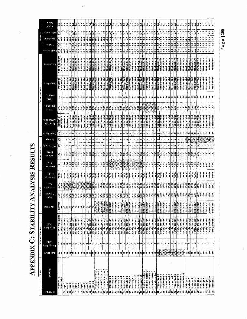
AP

PE

ND

IX C

: ST

AB

ILIT

Y A

NA

LY

SIS

RE

SU

LT

S

1 I m

os

t ri

sk

y 2

! le

as

t ri

sk

y _

3_

jag

e 1

4 Ia

ge

2 5

i ag

e 3

6 7 8~

. 9

"10

"

"ii"

1

2 1

3 1

4 IS

1

6 17

~18

~ 1

9 ~

20

"

22

23

24

25

..._£

..

27

2S

~ 2

9_

j 3

0 3

1

32

33

34

35

36

37

38

39

_4

0 4

1

42

43

-1

44

45

46

47

"48

49

50

51

52

53

54

55

ag

e 4

ag

e 5

ag

e 6

ag

e 7

ag

e 8

ag

e 9

ag

e 1

0 a

ge

11

typ

e o

f m

ate

ria

l 2

typ

e o

f m

ate

ria

l 3

typ

e o

f m

ate

ria

l 4

typ

e o

f m

ate

ria

l 5

typ

e o

f m

ate

ria

l 6

bre

ak

ag

e 2

bre

ak

ag

e 3

bre

ak

ag

e 4

bre

ak

ag

e 5

bre

ak

ag

e 6

bre

ak

ag

e 7

bre

ak

ag

e 8

bre

ak

ag

e 9

bre

ak

ag

e 1

0 b

rea

ka

ge

11

bre

ak

ag

e 1

2 b

rea

ka

ge

13

pip

e d

iam

ete

r 2

pip

e d

iam

ete

r 3

pip

e d

iam

ete

r 4

pip

e d

iam

ete

rs

pip

e d

iam

ete

r 6

typ

e o

f so

il 2

typ

e o

f so

il 3

typ

e o

f so

il 4

typ

e o

f s

oil

5 .

typ

e o

f s

oil

6 ty

pe

of

soil

7 ty

pe

of

soil

8 ty

pe

of

soil

9 ty

pe

of

so

il 1

0 ty

pe

of

soil

11

lea

ka

ge

2 le

ak

ag

e 3

lea

ka

ge

4 le

ak

ag

e 5

lea

ka

ge

6 le

ak

ag

e 7

lea

ka

ge

8 le

ak

ag

e 9

lea

ka

ge

10

lea

ka

ge

11

10 o 0 0 0

~6~

0 o o 0 0 0 o 0 0 0 0 o o o 0 0 o 0 0 0 0 "6" 0 o 0 o o 0 0 1 10

. 1

0 1

0

" 1

0 1

0 id

10

10 10

10

10 0

_,

0 0 0 0 0 0 0 0 0 1

0 0 0

_ °

1 0 0 0 0 0 0 0

J 0 0 0 0 0

_]

0 0 0 0 0 0 0 0 0 0 0 0 0 0 0 0 0 0 0 0 0

" ~

d"~

' 0 0 0 0 0

se

as

on

all

y p

res

en

t ra

rely

p

res

en

t ra

rely

p

res

en

t ra

rely

p

res

en

t ra

rely

p

res

en

t ra

rely

p

res

en

t ra

rely

p

res

en

t ra

rely

p

res

en

t ra

rely

p

res

en

t ra

rely

p

res

en

t ra

rely

p

res

en

t ra

rely

p

res

en

t ra

rely

p

res

en

t ra

rely

p

res

en

t ra

rely

p

res

en

t ra

rely

p

res

en

t ra

rely

p

res

en

t ra

rely

p

res

en

t

rare

ly

pre

se

nt

rare

ly

pre

se

nt

rare

ly

pre

se

nt

rare

ly

pre

se

nt

rare

ly

pre

se

nt

rare

ly

pre

se

nt

rare

ly

pre

se

nt

rare

ly

pre

se

nt

rare

ly

pre

se

nt

rare

ly

pre

se

nt

rare

ty

pre

se

nt

rare

ly

pre

se

nt

rare

ly

pre

se

nt

rare

ty

pre

se

nt

rare

ly

pre

se

nt

rare

ly

pre

se

nt

rare

ly

pre

se

nt

rare

ly

pre

se

nt

rare

ly

pre

se

nt

rare

ly

pre

se

nt

rare

ly

pre

se

nt

rare

ly

pre

se

nt

rare

ly

pre

se

nt

rare

ly

pre

se

nt

rare

ly

pre

se

nt

rare

ly

pre

se

nt

rare

ly

pre

se

nt

rare

ly

pre

se

nt

rare

ly

pre

se

nt

rare

ly

pre

se

nt

. ra

rely

p

res

en

t ra

rely

p

res

en

t ra

rely

p

res

en

t ra

rely

p

res

en

t

rare

ly

pre

se

nt

rare

ly

pre

se

nt

rare

ly

pre

se

nt

Ca

st

iro

n P

E

PE

P

E

| P

E

PE

P

E

PE

P

E

j P

E

"•

PE

P

E

PE

' P

VC

C

on

cre

te

Asb

esto

s C

as

t ir

on

t ir

on

po

st

: ir

on

po

st

£ ir

on

po

st

; ir

on

po

st

t ir

on

po

st

: ir

on

po

st

: ir

on

po

st

: ir

on

po

st

i ir

on

po

st

t ir

on

po

st

t ir

on

po

st

: ir

on

po

st

c ir

on

po

st

: ir

on

po

st

t ir

on

po

st

t ir

on

po

st

t ir

on

po

st

t ir

on

po

st

c Ir

on

po

st

c ir

on

po

st

t ir

on

po

st

t ir

on

po

st

: ir

on

po

st

: ir

on

po

st

: ir

on

po

st

: Ir

on

po

st

l ir

on

po

st

: ir

on

po

st

: ir

on

po

st

: ir

on

po

st

: ir

on

po

st

: ir

on

po

st

: ir

on

po

st

: ir

on

po

st

[ ir

on

po

st

: ir

on

po

st

: ir

on

po

st

[ ir

on

po

st

10

0 5

00

50

0 5

00

"50

0 1

50

0 _,

5

00

50

0 5

00

50

0 5

00

50

0 5

00

50

0 5

00

50

0 5

00

50

0 5

00

50

0 5

00

50

0 5

00

50

0 5

00

j 5

00

50

0 5

00

50

0 5

00

1 3

50

30

0 2

50

20

0 1

50

15

0 1

50

15

0 1

50

15

0 1

50

15

0 1

50

15

0 1

50

l_

15

0 1

50

ISO

15

0 ~

" 1

50

" 1

50

15

0

15

0

15

0

ISO

19

00

20

07

20

07

19

97

19

87

19

77

19

67

19

57

J9

47

19

37

19

27

. 1

91

7 1

90

7 1

90

7 1

90

7 1

90

7 1

90

7 1

90

7 1

90

7 j

19

07

1 1

90

7 1

90

7 1

90

7 1

90

7 1

90

7 1

90

7 j

19

07

19

07

j 1

90

7^

19

07

19

07

19

07

19

07

19

07

19

07

19

07

19

07

19

07

19

07

19

07

19

07

19

07

19

07

19

07

19

07

19

07

19

07

19

07

19

07

19

07

19

07

19

07

19

07

19

07

19

07

no

ne

no

ne

no

ne

no

ne

no

ne

no

ne

no

ne

no

ne

no

ne

no

ne

no

ne

no

ne

no

ne

no

ne

no

ne

no

ne

no

ne

no

ne

no

ne

no

ne

no

ne

no

ne

no

ne

no

ne

no

ne

no

ne

no

ne

no

ne

no

ne

no

ne

no

ne

no

ne

no

ne

no

ne

no

ne

no

ne

no

ne

no

ne

no

ne

no

ne

no

ne

no

ne

no

ne

no

ne

no

ne

no

ne

no

ne

no

ne

no

ne

no

ne

no

ne

no

ne

no

ne

no

ne

no

ne

6 0 0

.00

0.0

0 0

.00

°-°<

J_

J 0

.00

0.0

0 00

0__J

0.0

0 0

.00

0.0

0 0

.00

0.0

0 0

.00

0.0

0 0

.00

d.oo

0

.25

0.5

0 0

.7S

too

2.0

0 2

.25

2.5

0 2

.75

3.0

0 3

.25

3.5

0 4

.00

. 4

.00

4.0

0 4

.00

4.0

0 4

.00

4.0

0 4

.00

4.0

0 4

,00

4.0

0 4

.00

4.0

0 4

.00

4.0

0 4

.00

4.0

0 4

.00

'" 4

.00

""

4.0

0 4

.66

4.0

0 4

.00

4.0

0

4.0

0

4.0

0

30

13

0 1

30

13

0 1

30

13

0 1

30

13

0 1

30

13

0 1

30

13

0 1

30

13

0 !_

_1

30

13

0

r i3

o 1

30

13

0 1

30

13

0 1

30

13

0 1

30

13

0 [

13

0 1

30

13

0 1

30

13

0 1

30

13

0 1

30

13

0 1

30

13

0 1

30

13

0 1

30

13

0 1

30

13

0 1

30

13

0 1

30

13

0

t 1

3°

13

0 1

30

" 1

30

"

, 1

30

13

0 1

30

13

0

13

0

10 0 0 0 o 0 0 o 0 0 o o o o 0 0 0 0

1 0 0 0 0 0 o 0 0 cT

^ 0 0 0 0 0 0 0 0 0 0 0 o o 0 o 0 o o 0

" 0 0 0 o o 0 0 °

10 0 0 0 o 0 0 0 o o 0 0 o o o o 0 o o 0 0 0 0 0 0 o 0 0 0 0 0 0 0 0 o 0 0 0 0 0 0 0 0 0 o

i , -*— .*

. .

9 a« —

o 0 0 0 0 0 0 0 0 0 0 o 0 0 0 0 o 0 0 0 0 0 0 0 o o o o o o o 0 o o 0 0 o 0 0 0 0 o 0 o o 0 0 0 0 0 0 0 9..

.

Ind

us

tria

l R

es

ide

nti

al

Re

sid

en

tia

l R

es

ide

nti

al

Re

sid

en

tia

l R

es

ide

nti

al

Re

sid

en

tia

l R

es

ide

nti

al

Re

sid

en

tia

l R

es

ide

nti

al

Re

sid

en

tia

l R

es

ide

nti

al

Re

sid

en

tia

l R

es

ide

nti

al

Re

sid

en

tia

l R

es

ide

nti

al

Re

sid

en

tia

l R

es

ide

nti

al

Re

sid

en

tia

l R

es

ide

nti

al

Re

sid

en

tia

l R

es

ide

nti

al

Re

sid

en

tia

l R

es

ide

nti

al

Re

sid

en

tia

l R

es

ide

nti

al

Re

sid

en

tia

l R

es

ide

nti

al

Re

sid

en

tia

l R

es

ide

nti

al

Re

sid

en

tia

l R

es

ide

nti

al

Re

sid

en

tia

l R

es

ide

nti

al

Re

sid

en

tia

l R

es

ide

nti

al

Re

sid

en

tia

l R

es

ide

nti

al

Re

sid

en

tia

l R

es

ide

nti

al

Re

sid

en

tia

l R

es

ide

nti

al

Re

sid

en

tia

l R

es

ide

nti

al

Re

sid

en

tia

l R

es

ide

nti

al

Re

sid

en

tia

l

Re

sid

en

tia

l R

es

ide

nti

al

Re

sid

en

tia

l R

es

ide

nti

al

Re

sid

en

tia

l

Re

sid

en

tia

l

Re

sid

en

tia

l

Re

sid

en

tia

l

10

0 5

00

50

0 5

00

50

0 5

00

50

0 5

00

50

0 5

00

50

0 5

00

50

0 5

00

50

0 5

00

50

0 5

00

50

0 5

00

50

0 5

00

50

0 5

00

50

0 5

00

50

0 5

00

50

0 5

00

35

0 3

00

* 2

50

, 2

00

"'•

i£d

ISO

1

50

15

0

15

0 1

50

15

0 1

50

15

0 1

50

15

0 1

50

15

0 1

50

15

0 1

50

15

0 1

50

15

0

15

0

15

0

10 0 0 0 0 0 0 0 0 0 0 0 0 0 0 0 0 b 0 0 0 0 0 0 0 0 0 0 0 0 0 0 0 0 0 0 0 0 0 0 0 0 0 0 0 0 0 0 0 0 0 0 0 0

Ind

us

tria

l R

es

ide

nti

al

Re

sid

en

tia

l R

es

ide

nti

al

Re

sid

en

tia

l R

es

ide

nti

al

Re

sid

en

tia

l R

es

ide

nti

al

Re

sid

en

tia

l R

es

ide

nti

al

Re

sid

en

tia

l R

es

ide

nti

al

Re

sid

en

tia

l R

es

ide

nti

al

Re

sid

en

tia

l R

es

ide

nti

al

Re

sid

en

tia

l R

es

ide

nti

al

Re

sid

en

tia

l R

es

ide

nti

al

Re

sid

en

tia

l R

es

ide

nti

al

Re

sid

en

tia

l R

es

ide

nti

al

Re

sid

en

tia

l R

es

ide

nti

al

Re

sid

en

tia

l R

es

ide

nti

al

Re

sid

en

tia

l R

es

ide

nti

al

Re

sid

en

tia

l R

es

ide

nti

al

Re

sid

en

tia

l R

es

ide

nti

al

Re

sid

en

tia

l R

es

ide

nti

al

Re

sid

en

tia

l R

es

ide

nti

al

Re

sid

en

tia

l R

es

ide

nti

al

Re

sid

en

tia

l R

es

ide

nti

al

Re

sid

en

tia

l R

es

ide

nti

al

Re

sid

en

tia

l R

es

ide

nti

al

Re

sid

en

tia

l R

es

ide

nti

al

Re

sid

en

tia

l R

es

ide

nti

al

Re

sid

en

tia

l R

es

ide

nti

al

Re

sid

en

tia

l

Re

sid

en

tia

l

Re

sid

en

tia

l

No

t R

ed

un

de

nt

Re

du

nd

en

t

Re

du

nd

en

t R

ed

un

de

nt

Re

du

nd

en

t R

ed

un

de

nt

Re

du

nd

en

t R

ed

un

de

nt

Re

du

nd

en

t R

ed

un

de

nt

Re

du

nd

en

t R

ed

un

de

nt

Re

du

nd

en

t R

ed

un

de

nt

Re

du

nd

en

t R

ed

un

de

nt

Re

du

nd

en

t R

ed

un

de

nt

Re

du

nd

en

t R

ed

un

de

nt

Re

du

nd

en

t R

ed

un

de

nt

Re

du

nd

en

t R

ed

un

de

nt

Re

du

nd

en

t R

ed

un

de

nt

Re

du

nd

en

t R

ed

un

de

nt

Re

du

nd

en

t R

ed

un

de

nt

Re

du

nd

en

t R

ed

un

de

nt

Re

du

nd

en

t R

ed

un

de

nt

Re

du

nd

en

t R

ed

un

de

nt

Re

du

nd

en

t R

ed

un

de

nt

Re

du

nd

en

t R

ed

un

de

nt

Re

du

nd

en

t R

ed

un

de

nt

Re

du

nd

en

t R

ed

un

de

nt

Re

du

nd

en

t R

ed

un

de

nt

Re

du

nd

en

t R

ed

un

de

nt

Re

du

nd

en

t R

ed

un

de

nt

Re

du

nd

en

t R

ed

un

de

nt

Re

du

nd

en

t

Re

du

nd

en

t

Re

du

nd

en

t

—

0.6

0

.6

0.6

0

.6

0.6

0

.6

0.6

0

.6

0.6

0

.6

0.6

0

.6

0.6

0

.6

0.6

0

.6

0.6

0

.6

0.6

0

.6

0.6

0

.6

0.6

0

.6

0.6

0

.6

0.6

0

.6

0.6

0

.6

0.6

0

.6

0.6

0

.6

1.3

1.5

2.1

2

.6

3.3

4

.1

4.5

5

.0

5.0

5

.0

5.0

5

.0

5.0

5

.0

5.0

5

.0

5.0

5.0

5.0

_L°-

8.3

1

.7

1.7

1.7

1.8

2

.6

3.5

4

.2

5.0

5

.0

5.0

5

.0

5.0

5

.0

6.7

6

.7

6.7

8

.3

8.3

8

.3

8.3

8

.3

8.3

8

.3

8.3

8

.3

8.3

8

.3

8.3

8

.3

8.3

8

.3

8.3

8

.3

8.3

8

.3

8.3

8

.3

8.3

8

.3

8.3

8

.3

8.3

8

.3

8.3

8

.3

8.3

8.3

8

.3

8.3

8

.3

8.3

8.3

8.3

JL2.

9.4

0

.6

0.6

0

.6

0.6

0

.6

0.6

0

.6

0.6

0

.6

0.6

0

.6

0.6

0

.6

0.6

0

.6

0.6

0

.6

1.1

1.

3 1.

5 1.

7 1.

7 1.

7 1.

7 2

.2

2.5

2

.8

3.3

3

.3

3.3

3

.3

3.3

3

.3

3.3

3

.3

3.3

3

.3

3.3

3

.3

3.3

3

.3

3.3

3

.3

3.3

4

.1

4.5

5

.0

5.0

5

.0

5.7

6

.2

6.7

6.7

6.7

8.3

1

.7

1.7

1.

7 1

.7

1.7

1

.7

1.7

1.7

1.7

1

.7

1.7

1.7

1.7

1.7

1.

7 1.

7 1.

7 1.

7 1.

7 1.

7 1.

7 1.

7 1.

7 1.

7 1.

7 1.

7 1.

7 1.

7 1.

7 1.

7 1.

7 1.

7 1

.7

1.7

1.7

1.7

1.

7 1.

7 1

.7

1.7

1.7

1.7

1.7

1.7

1.7

1.

7 1.

7 1.

7 1.

7 1.

7 1.

7

1.7

1.7

12-

8.3

1

.7

1.7

1

.7

1.7

1

.7

1.9

2

.4

2.3

2

.3

2.3

2

.3

2.3

2

.3

3.3

3

.3

3.3

4

.0

4.0

4

.0

4.0

4

.0

4.0

4

.0

4.0

4

.0

4.2

4

.4

5.0

5

.0

5.0

5

.0

S.O

5

.0

5.0

5

.0

5.0

5

.0

5.0

5

.0

5.0

5

.0

S.O

5

.0

5.0

5

.0

5.0

5

.0

5.0

5

.0

5.8

6

.1

6.7

6.7

6.7

Pa

ge

| 200

6.7

1.

7

6.7

8.3

5.0

R

edundent

Resid

ential

o

150

R

esid

ential

o

a r »

130

4.0

0

none

150

j

1907

t iron

post

rare

ly p

resent

o

o r-t

6.7

1.

7

6.7

8.3

5.0

R

edundent

Resid

ential

o

150

R

esid

ential

o

o «-t

«

130

4.0

0

none

150

!

1907

t iron

post

rare

ly p

resent

o

a

6.7

1.

7

6.7

8.3

5.0

R

edundent

Resid

ential

o

150

R

esid

ential

o

o r-l

WJ

130

4.0

0

none

1907

150

t iron

post

rare

ly p

resent

o

o r-t

6.7

1.

7

6.7

8.3

5.0

R

edundent

Resid

ential

o

150

R

esid

ential

O

o r-l

*

130

4.0

0

none

1907

150

t iron

post

rare

ly p

resent

o

o r-t

6.7

1.

7

6.7

8.3

5.0

R

edundent

Resid

ential

o

150

R

esid

ential

o

o r-l

in

130

4,0

0

none

1907

150

t iron

post

rare

ly p

resent

o

o

6.7

1.

7

7.4

8.3

S R

edundent

Resid

ential

o

150

R

esid

ential

o

o

«

4.0

0

j 130

none

1907

0SI

t iron

post

0

! ra

rely

pre

sent

a

6.7

1.

7

7.9

8.3

5.0

R

edundent

Resid

ential

o

150

R

esid

ential

o

o

N

4.0

0

| 130

none

1907

150

t iron

post

0

| ra

rely

pre

sent

o

6.7

1.7

8.3

8.3

5.0

R

edundent

Resid

ential

o

150

R

esid

ential

o

o

00

4.0

0

' 130

none

150

I

1907

t iron

post

c V s a

> IB

O

o f »

6.7

1.

7

8.3

8.3

5.0

R

edundent

Resid

ential

o

150

R

esid

ential

o

o

CI

4.0

0 I

130

none

150

'

1907

t iron

post

!

!

6.7

1.

7

£'8

8.3

5.0

R

edundent

Resid

ential

o

150

R

esid

ential

o

o

g

4.0

0

1

130

none

150

!

1907

c iron

post

rare

ly p

resent

o o

wa

ter

qualit

y 2

wa

ter qualit

y 3

wa

ter

qualit

y 4

wa

ter

qualit

y 5

wa

ter

qualit

y 6

wa

ter

qualit

y 7

wate

r qualit

y 8

wa

ter

qualit

y 9

wa

ter

qualit

y 1

0

wa

ter qualit

y 11

in »n m -i 1 H N

tojio to u>«c

6.7

3.3

8.

3 8.

3 5.0

R

edundent

Resid

ential

o

150

1 6 e 3 O

O r-t

O

4.0

0

i 13

0

none

150

i

1907

C iron

post

S !

o

a

6.7

3.3

8.

3 8.3

3

Redundent

Resid

ential

o

150

3s

C,

o

o

o r-l

4.0

0

f 130

150

i

1907

i

none

t iron

post

10 ;

0

|

rare

ly p

resent

dam

age t

o s

urr

oundin

g 2

dam

age t

o s

urr

oundin

g 3

u, £

6.7

3.3

8.3

8.

3 5.0

R

edundent

Resid

ential

o

150

in

dustr

ial

rt

O . - I

o

4,0

0

1

130

none

150

I

1907

t iron

post

rare

ly p

resent

o

o

6.7

3.

3 8.3

8.3

5.0

R

edundent

Resid

ential

o

150

In

dustr

ial

« o

o r-f

0£T

4.0

0

none

150

j

1907

t iron

post

rare

ly p

resent

0

i O

X

6.7

!

3.8

8.

3 8.3

o-s

Redundent

Resid

ential

o

150

In

dustr

ial

m

o i-l

o r-l

130

4.0

0

none

1907

150

C iron

post

rare

ly p

resent

o

s

6.7

4.3

8.

3 8.3

5.0

R

edundent

Resid

ential

o

150

In

dustria

l

V

o

o r-t

0£T

4.0

0

none

1907

150

t iron

post

rare

ly p

resent

o

o

6.7

5.0

£•8

8.3

5.0

R

edundent

Resid

ential

o

150

In

dustr

ial

i n

o i- l

o

130

4.0

0

none

1907

150

t iron

post

rare

ly p

resent

o

o

6.7

5.0

8.3

8.3

5.0

R

edundent

Resid

ential

o

150

In

dustria

l

©

o

o r-l

130

00'fr

none

1907

150

t iron

post

rare

ly p

resent

o

o r-t

6.7

5.0

8.

3 8.3

5.0

R

edundent

Resid

ential

o

150

In

dustria

l

** o

s

130

4.0

0

none

1907

150

C iron

post

rare

ly p

resent

o

o

6.7

5.0

8.

3 8.3

5.0

R

edundent

Resid

ential

o

150

In

dustria

l

M

o i-t

o 1-1

130

001?

none

1907

150

t iron

post

rare

ly p

resent

o

o

6.7

5.0

8.

3 8.3

5.0

R

edundent

Resid

ential

o

150

In

dustria

l

m

o

o i-l

130

4.0

0

none

1907

1

150

t iron

post

rare

ly p

resent

o

a

6.7

5.0

8.3

8.3

5.0

R

edundent

Resid

ential

o 150

In

dustria

l

*•* o r-t

O r-t

130

4.0

0

none

1907

150

o a c 0

rare

ly p

resent

o

o f t

cost of

repair 2

co

st of re

pair 3

cost of re

pair 4

co

st of

rep

air

s

cost of re

pair 6

cost

of re

pa

ir 7

cost of re

pa

ir 8

cost of re

pair 9

cost

of re

pa

ir 1

0

cost of re

pair 11

» m o to UD h-L..,I,_L

m r^

* U B * L

6.7

5.0

8.

3 8.3

6.7

R

edundent

Resid

ential

o

0ST

Industria

l

o

o r-t

o

OCT

4.0

0

none

1907

150

t iron

post

IE « a

I 1 o

o I-I

8.3

5.0

8.

3 8.3

8.3

R

edundent

Resid

ential

o

150

In

dustria

l

o r-l

o r-t

O i-l

130

4.0

0

none

1907

150

0 Q c 0

 !

o

o r-f

Wa

ter

tab

le level 2

W

ate

r ta

ble

level 3

£

8.3

6.7

8.

3 8.3

8.3

c

c

•Q w or

s z

Resid

ential

o

ost

Industr

ial

o T-4

o

o

130

4.0

0

none

1907

150

t iron

post

seasonally

pre

sent

o

a

Loss

of P

roduction

2

!

8.3

6.

7 8.3

8.3

8.

3 N

ot

Redundent

Resid

ential

H

150

In

dustria

l

o

o

o T-4

130

4.0

0

none

1907

150

t iron

post

se

aso

na

lly p

resent

o

o

8.3

6.7

8.

3 8.3

8.

3 N

ot

Redundent

Resid

ential

r*j

150

,

Industria

l

s s 2

130

4.0

0

none

o en

r-t

O

in

t iron

post

se

aso

na

lly p

resent

°

8.3

6.7

8.3

8.3

8.3

N

ot

Redundent

Resid

ential

« i

150

In

dustria

l

s s s

130

4.0

0

none

1907

IS

O

t iron

post

seasonally

pre

sent

o

8.3

6.7

8.

3 8.3

8.3

N

ot

Redundent

Resid

ential

<*

150

In

dustria

l

o

o

o

0£t

4.0

0

none

1907

IS

O

t iron

post

se

aso

na

lly p

resent

o

8.3

6.7

8.3

8.3

8.3

N

ot

Redundent

Resid

ential

*n

150

In

dustria

l

o

o

O

OST

4.0

0

none

150

1

19071

t iron

post

se

aso

na

lly p

resent

o

o j o i o S o r-T r-t j r-t 1 r-t

8.3

7.4

8.3

8.3

8.

3 N

ot

Redundent

Resid

ential

<o

150

in

dustr

ial

s s s

130

4.0

0

none

150

j

1907

t iron

post

se

aso

na

lly p

resent

o

o

8.3

7.9

8.

3 8.3

8.3

N

ot

Redundent

Resid

ential

*»

150

In

dustria

l

a a a

OS

I 4.0

0

none

1907

150

t iron

post

se

aso

na

lly p

resent

10 i

0

.

8.3

8.3

8.

3 8.3

8.3

N

ot

Redundent

Resid

ential

t o

150

In

dustria

l

s s s

130

4.0

0

none

1907

150

t iron p

ost

seasonally

pre

sent

o

o r-l

8.3

8.3

8.3

8.3

8.3

N

ot

Redundent

Resid

ential

0 !

150

In

dustria

l a s s

130

4.0

0

none

1907

150

t iron

post

se

aso

na

lly p

resent

o

o r-l

8.3

8.3

8.

3 8.3

8.3

N

ot

Redundent

Resid

ential

9

150

In

dustria

l o r-f

o r-l

o

130

4.0

0

none

1907

150

t iron

post

seasonally

pre

sent

o

o r-t

Tra

ffic

dis

ruption

2

Tra

ffic

dis

ruption

3

Tra

ffic

dis

ruption

4

Tra

ffic

dis

ruption

5

Tra

ffic

dis

ruption

6

Tra

ffic

dis

ruption

7

Tra

ffic

dis

ruption

8

Tra

ffic

dis

ruption

9

Tra

ffic

dis

ruption

10

Tra

ffic

dis

ruption

11

r-»

» 00 OOjOO 00 CO 00 4 0> O 00 CD

8.3

8.3

8.3

8.3

8.3

N

ot

Redundent

Resid

ential

o f t

150

In

dustria

l

o

s o r-t

8.3

8.3

8.3

8.3

8.3

N

ot

Redundent

Resid

entia

l

o

150

In

dustria

l

s a a

8.3

8.3

8.3

8.3

8.3

N

ot

Redundent

Resid

ential

o t-t

150

In

dustria

l

o r-l

o

o 8.3

8.3

8.3

8.3

8.3

N

ot

Redundent

Resid

ential

o r-l

150

In

dustria

l

o r-t

O H

O

8.3

8.3

8.3

8.3

8.3

N

ot

Redundent

Resid

ential

o

150

In

dustria

l

o r-t

o r-l

O r-l

8.3

8.3

8.3

8.3

8.3

N

ot

Redundent

Resid

ential

o i-t

150

In

dustria

l

o r-t

8.3

8.3

8.7

8.3

8.3

N

ot

Redundent

Resid

ential

o

150

o r-l

O O r-l W

O O riri

8.3

8.3

9.4

8.3

8.

3 N

ot

Redundent

Resid

ential

o r-l

150

In

dustria

l

o r-l

o

o r-l

8.3

8.3

9.4

8.3

8.3

N

ot

Redundent

Resid

ential

o r-t

150

In

dustria

l

o

g

o

8.3

8.3

9.4

8.3

8.3

N

ot

Redundent

Resid

ential

o

150

In

dustria

l

o r-t

o r-l

O

S 2 2 o o o ' o o c a 3 S S n » r»,<o W|<r(m

4.a

none

1907

150

c iron

post

seasonally

pre

sent

o

o

4.0C

none

1907

IS

O

t iron

post

seasonally

pre

sent

o

o

4.C

K

none

1907

150

t iron

post

seasonally

pre

sent

o

o r-t

4.0X

none

1907

15

0

t iron

post

seasonally

pre

sent

o

s

4.0

( none

1907

150

t iron

post

seasonally

pre

sent

o

o r-t

4.C

X

none

1907

150

t iron

post

seasonally

pre

sent

o

o r-l

4.0C

none

1907

150

t iron

post

seasonally

pre

sent

o

o r-t

4.0£

none

1907

0SX

t iron

post

seasonally

pre

sent

o

o r-l

4.0

( none

1907

150

t iron

post

seasonally

pre

sent

o

o r-t

4.0C

none

1907

150

t iron

post

seasonally

pre

sent

o

o r-t

Hydra

lic fa

cto

r 2

Hydra

lic facto

r 3

Hydra

lic facto

r 4

Hydra

lic f

acto

r 5

Hydra

lic facto

r 6

Hydra

lic facto

r 7

Hydra

lic facto

r 8

Hydra

lic facto

r 9

Hydra

lic facto

r 10

Hydra

lic fa

cto

r 11

« • m 1 •* i m enicnjen. •

M o o

5

ooi

8.3

8.3

9.4

8.3

8.3

N

ot

Redundent

5 o r-t

150

In

dustria

l

o r-l

o r-l

o r-l

O m

4.0

0

none

1907

150

t iron

post

seasonally

pre

sent

o

s

8.3

8.3

9.4

8.3

8.3

N

ot

Redundent

O T-t

150

In

dustria

l

o

o r-t

O rH

O m

4.0

0

none

1907

150

t iron

post

seasonally

pre

sent

o

"

Type o

f se

rive

d a

rea 2

Type o

f serived

are

a 3

m 1

02

8.3

8.3

9.4

8.3

8.3

N

ot

Redundent

industria

l

o r-l

150

In

dustria

l

o r-t

o

o 1-1

o

4.0

0

none

1907

150

t iron

post

seasonally

pre

sent

... a

8.3

8.3

9.4

8.3

8.3

N

ot

Redundent

Industria

l

s

150

In

dustria

l

o

o r-l

o t-t

o m

4.0

0

none

1907

150

t iron

post

seasonally

pre

sent

r*

*

8.3

8.3

9.4

8.3

8.3

N

ot

Redundent

Industria

l

o

150

j

Industria

l

o i-i

a o

o

4.0

0

none

1

90

7,

150

t iron

post

seasonally

pre

sent

m

o «-t

8.3

8.3

9.4

8.3

8.3

N

ot

Redundent

Industria

l

o

150

In

dustria

l

o

o

o

o m

4.0

0

none

1907

150

t iron

post

seasonally

pre

sent

*

o

-1

8.3

8.3

9.4

8.3

8.3

N

ot

Redundent

Industria

l

s

150

In

dustria

l

o r-t

o r-l

s

o m

4.0

0

none

1907

1

150

t iron

post

seasonally

pre

sent

i n

o r-t

8.3

8.3

9.4

8.3

8.6

N

ot

Redundent

Industria

l

3

150

In

dustria

l

o r-l

o r-l

o f t

o CO

4.0

0

none

1907

150

[ iron

post

seasonally

pre

sent

« t

o r-t

8.3

8.3

9.4

8.3

9.0

N

ot

Redundent

Industria

l

a

150

In

dustria

l

o

o t - i

s

o m

4.0

0

none

1907

150

t iron

post

c V <5 a >•

a c o to 0)

t s

o r-l

8.3

8.3

9.4

8.3

9.4

N

ot

Redundent

Industria

l

o r-t

OST

Industria

l

o r-t

o r-t

O

O

4.0

0

none

1907

150

: iron

post

seasonally

pre

sent

60

o

8.3

8.3

9.4

8.3

9.4

N

ot

Redundent

Industria

l

o r-l

150

In

dustria

l

o r-t

o r-t

o

o m

4.0

0

none

1907

150

t iron

post

seasonally

pre

sent

<h

o r-l

8.3

8.3

9.4

8.3

9.4

N

ot R

edundent

.2

£

o

150

In

dust

rial

o

o

o r-t

o

4.00

" '

none

19

07

150

: iron

post

se

ason

ally

pre

sent

a

a

illiliiiii Ifltllffl! £0T 10

4

105

106

107

108

109

110

111

Tl2

l

0/j

evaluating the risk of water main failure using a

Documents