IN DEGREE PROJECT ENVIRONMENTAL ENGINEERING,SECOND CYCLE, 30 CREDITS

, STOCKHOLM SWEDEN 2016

Evaluating the benefit-cost ratio of groundwater abstraction for additional irrigation water on global scale

MOHAMMAD FAIZ ALAM

KTH ROYAL INSTITUTE OF TECHNOLOGYSCHOOL OF ARCHITECTURE AND THE BUILT ENVIRONMENT

i

Evaluating the benefit-cost ratio of

groundwater abstraction for additional

irrigation water on global scale

Mohammad Faiz Alam

DEGREE PROJECT NO. 2016:23

KTH ROYAL INSTITUTE OF TECHNOLOGY

DIVISION OF LAND AND WATER RESOURCES ENGINEERING

SE-100 44 STOCKHOLM, SWEDEN

ii

TRITA-LWR Degree Project ISSN 1651-064XLWR-EX-2016:23

iii

Summary in English

Projections show that to feed a growing population which is expected to reach 9.1 billion in 2050 would require raising overall food production by some 70 percent by 2050. One of the possible ways to increase agricultural production is through increasing yields by expanding irrigation. This study assesses the potential costs and benefits associated with sustainable groundwater abstraction to provide for irrigation.

The feasibility of groundwater abstraction is determined using a combination of three indicators: groundwater recharge, groundwater quality (salinity) and sustainability (no depletion). Global groundwater recharge estimates used, are simulated with the Lund-Potsdam-Jena dynamic global vegetation model with managed lands (LPJmL). The cost of groundwater abstraction is determined on a spatially explicit scale on global level at a grid resolution of 0.5°. Groundwater abstraction cost is divided into two parts: capital costs and operational costs. The potential benefit of increased water supply for irrigation is given by the water shadow price which is determined by using a Model of Agricultural Production and its Impact on the Environment (MAgPIE). The water shadow price for water is calculated in areas where irrigation water is scarce based on the potential increase in agricultural production through additional water and it reflects the production value of an additional unit of water. The water shadow price is given on a 0.5° grid resolution in US $/m3. Combining the cost of abstraction and the water shadow price, the benefit cost ratio is calculated globally on a spatially explicit scale to determine where investment in groundwater irrigation would be beneficial. Finally, the results are analysed in global, regional and country perspectives.

The results show that groundwater abstraction is beneficial for an area of 135 million hectares which is around 8.8% of the total crop area in the year 2005. Europe show the highest potential with an area of ~ 50 million hectares with a majority of the area located in France, Italy, Germany and Poland. Second is North America with an area of ~ 43.5 million hectares located in the Eastern states where the irrigation infrastructure is less developed as compared to the Western states. Sub-Saharan Africa shows a potential of ~ 15.4 million hectares in the Southern and Eastern countries of Zimbabwe, Kenya, Malawi, Tanzania, Ethiopia and some parts of South Africa. South Asia despite extensive groundwater extraction shows only a moderate potential of ~ 9 million hectares, mostly located in India whereas China shows almost no potential. This is due to extensive groundwater depleted areas which were removed from the analysis and low water shadow prices which made abstraction not beneficial. Well installation costs play an important role in developing countries in regions of Sub-Saharan Africa and South Asia, where a reduction in costs would lead to an increase in area by more than 30%. Subsidy analyses shows that substantial increase in crop land areas where a benefit cost ratio >1 takes place in India with subsidised energy prices but this effect is found to be negligible in Mexico.

This study is, to the author’s knowledge, the first to assess the benefit cost ratio of groundwater

abstraction on a global scale by determining spatially explicit abstraction costs. The results show

that a great potential for groundwater abstraction exists in all regions despite problems of

groundwater depletion due to disparity in distribution and development of groundwater resources.

Energy subsidies and cheap well installation techniques are the two factors that could bring down

the abstraction costs which are quite important in developing regions where farm incomes are low.

Also, groundwater irrigation potential not only exists in arid areas of Africa and South Asia where

irrigation is needed but also in humid areas of Europe and North America where groundwater

irrigation can play an important role in building resilience to events of drought. However, it is

essential to not to follow the path that has led to groundwater depletion in many parts of the world

and develop this potential in a sustainable way through groundwater use regulations, policies and

efficient technologies.

Key words

Groundwater, Irrigation, Abstraction, Cost-benefit analysis, Global

iv

Summary in Swedish

Prognoser visar att för att föda en växande befolkning, som förväntas att uppgå 9,1 miljarder år 2050,

skulle det krävas en ökning av den totala livsmedelsproduktionen med cirka 70 procent fram till 2050.

Ett av de möjliga sätten för att öka jordbruksproduktionen är genom att öka avkastningen, vilket kan

ske genom att utöka bevattningen. Denna undersökning bedömer de potentiella kostnaderna och

fördelarna rörande hållbart uttag av grundvatten för att utnyttjas för bevattning.

Genomförbarheten av ett sådant grundvattenuttag bestämdes genom användning av en kombination av

tre indikatorer: grundvattenbildning, grundvattenkvalitet (salthalt) och hållbarhet (ingen utarmning).

Globala grundvattenbildningsuppskattningar som används numera simuleras med hjälp av Lund-

Potsdam-Jena dynamiska globala vegetationsmodell för behandlade länder (LPJmL). Kostnaden för

grundvattenuttag bestämdes på en rumsligt explicit skala på global nivå i ett rutnät med en upplösning

på 0,5°. Grundvattenuttagskostnaden var uppdelad i två delar: kapitalkostnader och driftskostnader.

Den potentiella fördelen med ökad tillgång av grundvatten för bevattning ges av det så kallade

vattenskuggpriset (WSP) som bestämdes genom att använda en modell av jordbruksproduktionen och

dess påverkan på miljön (Magpie). WSP för vatten beräknades i områden där bevattningen är knapp,

baserat på den potentiella ökningen av jordbruksproduktionen genom ytterligare bevattning och det

avspeglar produktionen av en ytterligare enhet av vatten. WSP beräknades över ett 0,5° rutnät i

US$/m3. Genom att kombinera kostnaden för uttag och WSP beräknades förmånskostnadskvoten

(BCR) globalt på en rumsligt explicit skala för att avgöra var investeringar i grundvattenbevattning

skulle vara fördelaktigt. Slutligen analyserades resultaten i globalt, regionalt och nationellt perspektiv.

Resultaten visade att grundvattenuttag skulle vara fördelaktigt för ett 135 miljoner hektar (MHA) stort

område, vilket är cirka 8,8 % av den totala odlingsarealen år 2005. Europa visade den högsta

potentialen med en ca 50 miljoner hektar stor yta och majoriteten av det området ligger i Frankrike,

Italien, Tyskland och Polen. Andra områden är i Nordamerika med en yta av ~ 43,5 miljoner hektar i de

östra staterna där bevattningsinfrastrukturen är mindre utvecklad jämfört med de västra staterna. I

Afrika söder om Sahara finns potential för 15,4 miljoner hektar i Zimbabwe, Kenya, Malawi, Tanzania,

Etiopien och några områden i Sydafrika. Trots omfattande uttag av grundvatten visar Sydasien endast

en måttlig potential på ~ 9 miljoner hektar främst belägna i Indien, medan Kina visar nästan ingen

potential. Detta beror på omfattande områden med utarmning av grundvatten, vilka därför uteslöts från

analyserna, och låga vattenskuggpriser som gjorde uttag olönsamt. Brunninstallationskostnaden spelar

en viktig roll i utvecklingsländer i regioner i Afrika söder om Sahara och södra Asien, där

kostnadsminskning skulle leda till en ökning av lämpliga områden med mer än 30 %.

Subventionsanalyser visar att en väsentlig ökning av markområden med grödor där BCR > 1 skulle

finnas i Indien med subventionerade energipriser, men effekten visade sig vara försumbar i Mexiko.

Denna undersökning är såvitt känt av författaren den första som bedömer nyttokostnadskvot för

grundvattenuttag på en global skala genom att bestämma rumsligt explicita abstraktionkostnader.

Resultaten visar att stora potentialer för grundvattenuttag finns i alla regioner trots problem med

grundvattenutarmning, på grund av skillnader i distribution och utveckling av grundvattenresurserna.

Energistöd och billig brunninstallationsteknik är de två faktorer som skulle kunna sänka

abstraktionskostnaderna, vilket är viktigt för utvecklingsregioner där jordbruksinkomsterna är låga.

Grundvattenbevattningspotential finns inte bara i torra områden i Afrika och Sydasien där bevattning

behövs men även i fuktiga områden i Europa och Nordamerika, där grundvattenbevattning kan spela en

viktig roll i att bygga resiliens mot perioder av torka. Men det är viktigt att utveckla denna potential på

ett hållbart sätt genom bestämmelser för användning av grundvatten, riktlinjer och effektivare teknik

och att undvika den väg som har lett till grundvattenutarmning i många delar av världen.

v

vi

Contents

Summary in English .......................................................................................................................... iii

Summary in Swedish ........................................................................................................................iv

Contents .............................................................................................................................................vi

List of Figures ....................................................................................................................................vi

List of Tables ...................................................................................................................................viii

1. Introduction ............................................................................................................................ 1

1.1 Irrigation .............................................................................................................................. 1

1.2 Groundwater resources ..................................................................................................... 2

1.3 Benefit cost ratio ................................................................................................................ 4

1.3.1 Groundwater abstraction cost ............................................................................................. 4

1.3.2 Potential benefit of groundwater abstraction ....................................................................... 5

1.4 Aim ....................................................................................................................................... 6

2. Theoretical and practical background ................................................................................. 6

2.1 Groundwater recharge ....................................................................................................... 6

2.2 Saline groundwater ............................................................................................................ 7

2.3 Groundwater depletion ...................................................................................................... 8

2.4 Irrigation-induced problems ............................................................................................. 8

2.5 Groundwater aquifer types ............................................................................................... 8

2.6 Groundwater abstraction cost .......................................................................................... 9

2.6.1 Capital costs ...................................................................................................................10

2.6.1.1 Pump types based on energy source .....................................................................10

2.6.1.2 Pump types based on operating principle ..............................................................11

2.6.1.3 Pump performance curves .....................................................................................12

2.6.1.4 Pump efficiency (p , m ) ......................................................................................13

2.6.1.5 Pump operating hours (T) ......................................................................................13

2.6.1.6 Pump maintenance and repair cost .......................................................................13

2.6.1.7 Pump installation cost ............................................................................................14

2.6.1.8 Equivalent annual cost ...........................................................................................15

2.6.2 Operational costs .......................................................................................................16

2.6.2.1 Electricity prices .....................................................................................................16

2.6.2.2 Energy subsidy .......................................................................................................16

2.6.2.3 Groundwater table depth ........................................................................................17

3 Methodology .........................................................................................................................18

3.1 Feasibility of groundwater abstraction ..........................................................................18

v

3.2 Groundwater abstraction costs ..................................................................................... 19

3.3 Benefit Cost Ratio............................................................................................................ 19

3.4 Sensitivity analysis ......................................................................................................... 19

3.4.1 Sensitivity to pump installation cost ............................................................................... 19

3.4.2 Electricity subsidy analysis ........................................................................................ 19

3.4.3 Sensitivity to groundwater recharge rates ................................................................. 19

4 Data ............................................................................................................. 19

4.1 Water shadow price ......................................................................................................... 19

4.2 Groundwater abstraction feasibility .............................................................................. 21

4.2.1 Groundwater recharge ................................................................................................... 21

4.2.2 Saline groundwater .................................................................................................... 23

4.2.3 Groundwater depletion .............................................................................................. 23

4.2.3.1 Country groundwater abstractions ......................................................................... 25

4.2.3.2 MAgPIE water use: Agriculture and other sectors ................................................. 26

4.2.3.3 Groundwater irrigation area ................................................................................... 28

4.2.3.4 Gridded groundwater abstractions ........................................................................ 30

4.2.3.5 Gridded groundwater depletion ............................................................................. 30

4.3 Groundwater abstraction costs ..................................................................................... 31

4.3.1 Capital costs .................................................................................................................. 31

4.3.1.1 Pump selection and price for analysis ................................................................... 31

4.3.1.2 Pump installation cost ............................................................................................ 33

4.3.1.3 Annuity of capital cost ............................................................................................ 34

4.3.2 Operational costs ....................................................................................................... 34

4.3.2.1 Electricity prices ..................................................................................................... 35

4.3.2.2 Pumping head (H) .................................................................................................. 36

4.3.2.3 Pump efficiency (p , m ) ..................................................................................... 37

4.3.2.4 Operating hours (T) ............................................................................................... 37

4.3.2.5 Maintenance and repair cost ................................................................................. 37

4.4 Aquifer types ...................................................................................................................... 37

5 Results and discussion ............................................................................. 38

5.1 Water shadow price ......................................................................................................... 38

5.2 Groundwater abstraction feasibility .............................................................................. 39

5.2.1 Overlap with yield increase potential ............................................................................. 42

vi

5.2.2 Overlap with aquifer types ..........................................................................................43

5.3 Groundwater abstraction cost ........................................................................................44

5.4 Benefit cost ratio ..............................................................................................................47

5.4.1 Sensitivity to installation cost .........................................................................................49

5.4.2 Subsidy analysis .........................................................................................................50

5.4.3 Sensitivity to recharge rates .......................................................................................51

5.5 Regional and country analysis .......................................................................................53

5.5.1 Europe ............................................................................................................................53

5.5.2 North America ............................................................................................................56

5.5.3 Sub-Saharan Africa ....................................................................................................57

5.5.4 South Asia and Centrally planned Asia including China ............................................58

5.5.5 Pacific Asia .....................................................................................................................59

5.5.6 Latin America .............................................................................................................60

5.6 Synthesis ..........................................................................................................................61

5.7 Limitations ........................................................................................................................61

6. Conclusion and recommendations .......................................................... 62

References ........................................................................................................... 64

Appendix .............................................................................................................. 70

Appendix 1: Country abstraction values ...................................................................................70

Appendix 2: Pump prices ............................................................................................................74

Appendix 3: Electricity prices: indexed to year 2005 ...............................................................75

Appendix 4: WaterGAP recharge ................................................................................................80

List of Figures

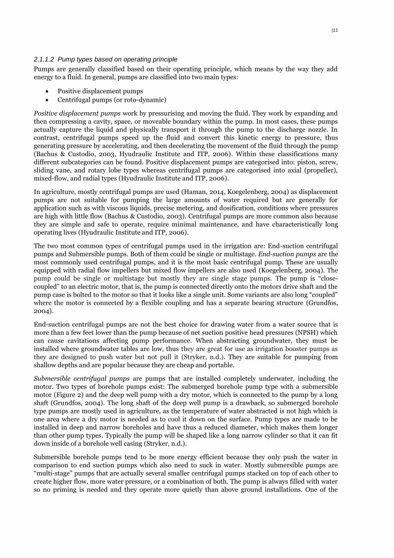
Figure 1: Electricity subsidy as % of country GDP for the year 2010 (Global Subsidy Initiative, 2010)5 Figure 2: Diagram showing submersible pumps installation structure (Sprinkler Irrigation System

Limited, n.d.) ...................................................................................................................................... 12 Figure 3: Pump performance curves. The orange line represents the Flow-Head relationship and the

green line represents the Flow-Efficiency relationship (Vogel, 2013). ............................................. 13

Figure 4: Energy subsidies in absolute amount (US $) and as percent of GDP for the world regions and

economies (Clements, et al., 2013, Sdralevich, Sab, Zouhar, & Albertin, 2014). ............................. 17

Figure 5: Flowchart of the conceptual framework illustrating the steps followed in the study .......... 18 Figure 6: Global classification of countries into 10 MAgPIE economic regions ................................ 20 Figure 7: The hydrology water routing scheme of LPJmL (Gerten et al. 2013). ............................... 22

Figure 8: Simulated average groundwater recharge by LPJmL in mm (1960-2000). Cell size of 0.5°.22

vii

Figure 9: Distribution of groundwater recharge (mm) in relation to crop land area in million hectares as

simulated by LPJmL for the period 1960-2000. ................................................................................. 23 Figure 10: Areas with high salt content in groundwater (>5 g/l).Cell size of 0.5° (WHYMAP, 2013).23 Figure 11: Flowchart of the conceptual framework illustrating the steps followed to derive the gridded

groundwater abstraction. ................................................................................................................... 25 Figure 12: Country groundwater abstractions in km

3 as derived from IGARC database for the year

2005. .................................................................................................................................................. 26 Figure 13: Country level agricultural water use (%) based on MAgPIE results for agricultural and total

water use. .......................................................................................................................................... 27 Figure 14: Water use sum in domestic, industrial and electrical production sectors. Cell size of 0.5°.27 Figure 15: Irrigated area as percent of total land area. Cell size of 0.5°. .......................................... 28

Figure 16: Percentage of irrigated area (Figure 9) equipped for groundwater Irrigation. Cell size of 0.5°.

........................................................................................................................................................... 29

Figure 17: Percentage groundwater equipped irrigated area in relation to total irrigated area per country.

........................................................................................................................................................... 30 Figure 18: Total groundwater abstractions in mm calculated as sum of groundwater abstractions in

agricultural and other sectors (domestic, industry, electricity production). Cell size of 0.5°. ............ 30 Figure 19: Groundwater depletion in mm calculated as difference between groundwater recharge and

abstractions. Cell size of 0.5°. ........................................................................................................... 31 Figure 20: Average of pump prices in US $ for different depth ranges in different countries/regions.33 Figure 21: Average pump prices in US $ for different depth ranges divided on the bases of countries

income level. ...................................................................................................................................... 33 Figure 22: Country electricity prices in US cents/kWh for year 2005. ............................................... 35

Figure 23: Pumping head in metres calculated as sum of groundwater table, friction loss and operating

head. Cell size of 0.5°. ....................................................................................................................... 37

Figure 24: Different aquifer types as produced by (WHYMAP (2015)). Cell size of 0.5°. ................. 38 Figure 25: Water shadow prices (WSP) in US cents/m

3. Cell size of 0.5°. ........................................ 39

Figure 26: Areas where groundwater abstraction is applicable based on criteria of recharge (>20 mm),

salt content (<5 g/l) and no groundwater depletion. Cell size of 0.5°. ............................................... 40 Figure 27: Available groundwater (mm) calculated after subtracting existing abstractions from

groundwater recharge for areas where groundwater abstraction is feasible. Cell size of 0.5°. ........ 41 Figure 28: Distribution of available groundwater (mm) in relation to crop land area in million hectares

(Mha) where groundwater abstraction is feasible. ............................................................................. 41

Figure 29: Water shadow prices (WSP) in US cents/m3

where groundwater abstraction is possible. Cell

size of 0.5°. ........................................................................................................................................ 42

Figure 30: Potential increase of rainfed crop yields (%) that would be possible with irrigation. Cell size of

0.5°. .................................................................................................................................................... 43 Figure 31: Distribution of potential Increase of rainfed crop yields (%) with irrigation in relation to crop

land in million hectares (Mha) where groundwater abstraction is feasible. ....................................... 43 Figure 32: Distribution of aquifer types in relation to crop land in million hectares (Mha) where

groundwater abstraction is feasible. .................................................................................................. 44 Figure 33: Total pumping cost in US cents/m

3 for scenarios with an installation cost of 50 US $/m (top),

100 US $/m (middle) and 200 US $/m (bottom) for the year 2005. Cell size of 0.5°. ....................... 45 Figure 34: Distribution of groundwater abstraction costs in US cents/m

3 for crop land area in Mha forthe

three scenarios with installation cost of US $50/m, US $ 100/m and US $ 200/m for the year 2005.46

Figure 35: Cost of pumping in US cents/m3 for the default scenario with installation cost of 100 US $/m,

where groundwater abstraction is possible and a water shadow price exists. Cell size of 0.5° ........ 47 Figure 36: Benefit cost ratio (BCR): 1) top with installation cost of 50 US $/m; 2) middle with installation

cost of 100 US $/m; 3) bottom with installation cost of 200 US $/m. Cell size of 0.5°. ..................... 48

viii

Figure 37: Area (Mha) and number of cells where BCR >1 for the three scenarios, with installation costs

of 50 US $/m, 100 US $/m and 200 US $/m. .................................................................................... 49 Figure 38: Area (Mha) for the three installation cost scenarios for 10 MAgPIE regions. Sub-

SaharanAfrica (AFR), Centrally Planned Asia Including China (CPA), Europe including Turkey (EUR),

the newly independent states of the former soviet Union (FSU), Latin America (LAM), Middle East/North

Africa (MEA), North America (NAM), Pacific OECD including Japan, Australia, New Zealand (PAO);

Pacific Asia (PAS) and South Asia Including India (SAS). ................................................................ 49 Figure 39: Cells with BCR >1 in India. 1) Left: installation cost 100 $/m and without subsidy; 2) middle:

installation cost 100 US$/m and with subsidy; 3) right: installation cost 50 $/m and with subsidy. Cell

size of 0.5°. ........................................................................................................................................ 50 Figure 40: Potential area (million hectares, Mha) in India for three scenarios with subsidy and cheap

installation cost. ................................................................................................................................. 51 Figure 41: Benefit cost ratio (BCR) with groundwater abstraction feasibility determined using WaterGAP

recharge rates. Cell size of 0.5°. ....................................................................................................... 52 Figure 42: Comparison of potential area (Mha) as determined using LPJmL and WaterGAP recharge

rates for 10 MAgPIE regions. Sub-Saharan Africa (AFR), ), Centrally Planned Asia Including China

(CPA), Europe including Turkey (EUR), the newly independent states of the former soviet Union (FSU),

Latin America (LAM), Middle East/North Africa (MEA), North America (NAM), Pacific OECD including

Japan, Australia, New Zealand (PAO); Pacific Asia (PAS) and South Asia Including India (SAS). . 52 Figure 43: Countries which contribute to more than 80% increase in potential area (Mha) determined

using WaterGAP recharge rates ....................................................................................................... 53

Figure 44: Area (Mha) where BCR >1 and percentage irrigated area for the 5 European countries with

the highest groundwater irrigation potential. ..................................................................................... 54

Figure 45: Water use statistics for irrigation and groundwater use for southern European countries.

Irrigation water use as percent of total water use in green and groundwater contribution to irrigation as

percent in blue. .................................................................................................................................. 54

List of Tables

Table 1: Groundwater abstraction estimates in different continents .................................................... 3

Table 2: Groundwater abstraction costs in US cents/m3 from literature .............................................. 9

Table 3: Pump installation costs for machine drilled borewell in US $/m gathered from literature. ..14

Table 4: Comparison of pumping costs (US cents/m ) with values reported in literature. .................46

ix

|1

1. Introduction

The world population is projected to increase by more than one billion people within the next 15 years,

reaching 8.5 billion in 2030, and to increase further to 9.7 billion in 2050, with most of this increase

concentrated in Asia and Africa (United Nations, 2015). Though population is expected to plateau

around 9 billion by 2050, this deceleration in population growth is correlated with increased wealth

which will provide higher purchasing power driving higher consumption and a greater demand for

processed food, meat, dairy, and fish, all of which add more pressure to the food supply system

(Godfray, et al., 2010). In order to feed this larger and richer population, food production must increase

by 70 percent. Annual cereal production will have to rise to about 3 billion tonnes from 2.1 billion today

(FAO, 2009). At the same time, agricultural producers will face a greater competition for land, water,

and energy resources from other sectors and an additional uncertainty from climate change effects.

To satisfy the growing worldwide demand for food, especially grains, two broad options are available: to

expand the area under production or to increase the productivity on existing cropland (Edgerton,

2009). Productivity could be increased by using new crop varieties and intensification of agriculture to

reduce yield gap through irrigation, fertilisers, land management etc. Both ways will have profound

impacts on the environment which needs to be factored in while deciding on the policy measures. More

intensive and industrialised agriculture impacts quality and quantity of surface water and groundwater,

and leads to soil erosion, pollution due to large-scale use of pesticides, and loss of habitats and

biodiversity (Walls, 2006). Expansion of cultivated land leads to forest encroachment and the resulting

loss of carbon sequestration and biodiversity that are critical global public goods (Laurance et al., 2104).

Expansion of cultivated land is expected to play a small part in the future according to the analysis that

accounts for suitability of remaining land for cropping and alternative land uses (Sadras, et al., 2015).

FAO expects that globally 90 percent (80 percent in developing countries) of the growth in crop

production will come from intensification of agricultural production leading to higher yields (FAO,

2009).

1.1 Irrigation

Yields have increased substantially after 1960’s due to intensified crop management involving improved

germplasm, greater inputs of fertilizer, production of two or more crops per year on the same piece of

land, and irrigation (Cassman, 1999). Irrigation is expected to play an increasingly important role in the

agricultural production of the developing countries. Irrigated agriculture is practiced on less than 20%

of the cultivated land but accounts for more than 40% of the world’s production (WWAP , 2012). Also,

the potential of increasing yields in rainfed agriculture is restricted owing to the reason that rainfall is

subjected to large seasonal and inter-annual variations and also carries a high risk of yield reductions or

complete loss of crop from dry spells and droughts (FAO, 2003). According to FAO estimates, the

developing countries have some 400 million hectares of land which, when combined with available

water resources and equipped for irrigation, represents a significant potential for irrigation extension.

About one half of this total 400 million (some 202 million hectares) is already equipped in varying

degrees for irrigation and the projections conclude that an additional 40 million hectares could come

under irrigated use, raising the total to 242 million ha in 2030 (FAO, 2003).

Already at present, irrigation accounts for more than 70% of the total water withdrawals and for more

than 90% of the total consumptive water use globally (Doll, 2009, WWAP, 2009). Expansion of

irrigation would lead to a 14 percent increase in water withdrawals for agriculture depending crucially

on the projected increase in irrigation water use efficiency (FAO, 2003). Though at global scale there are

sufficient water resources to support this, they are very unevenly distributed in space and time. Water

scarcity is becoming an important bottle neck with an increasing number of countries reaching alarming

levels of water scarcity and 1.4 billion people living in areas with sinking ground water levels (FAO,

2009). While supplies are scarce in many areas, there are ample opportunities to increase water use

efficiency and to tap undeveloped water resources for irrigation. According to a World Bank/FAO study,

irrigation currently represents a relatively small part of the total renewable water resources in many

|2

developing countries, and there remains a significant potential for further irrigation development

(Faurès, Hoogeveen, & Bruinsma, 2000).

To increase production, irrigation infrastructure must be extended into more crop areas and a larger

proportion of renewable freshwater must be utilised but in a more efficient and sustainable way. Water

for irrigation can be supplied through different measures and from different sources, such as canals and

dams from surface water, groundwater abstraction, wastewater reuse, desalination and rainwater

harvesting. This study focuses on the potential of groundwater abstraction. Groundwater plays an

essential role for irrigation as they are more reliable than surface water resources, are less prone to

pollution and present considerably less water shortage risk than surface water, as a result of the buffer

capacity of its relatively large volume (van der Gun, 2012).

1.2 Groundwater resources

In the past three to five decades, groundwater withdrawal has exponentially increased reflecting

humanity’s increased needs for food and industrial production because groundwater aquifers present a

source which is freely available and poorly subjected to regulation (UNESCO-IHP, 2009). According to

Shah et al., 2007, boom in groundwater development of agriculture started in Italy, Mexico, Spain &

USA in the early part of the century followed by South Asia, North China plain, and the Middle East in

the 1970’s and at present a third wave of increasing abstraction is taking place in many regions of Africa,

Srilanka and Vietnam. The intensification of smallholder agriculture in parts of Asia, Africa and Latin

America resulted in farmers installing their own low lift pumps to extract shallow groundwater

(Madramootoo, 2012). For example, in India the number of irrigation wells equipped with diesel or

electric pumps increased from 150,000 in 1950 to nearly 19 million by 2000 and in the Punjab region of

Pakistan from barely a few thousands to in 1960 to 0.5 million in 2000 (Shah, 2007).

At present groundwater is extensively used for irrigation in many parts of the world. According to

Siebert et al., 2010, 38% of the area equipped for irrigation was equipped with groundwater irrigation

contributing to total consumptive groundwater use of 545 km3/yr which was 43% of the total

consumptive irrigation water use. Döll, et al. (2011) using the global water resources and use model

WaterGAP estimated that groundwater withdrawals contributed to 35% of the water withdrawn

worldwide (approximately 1500 km3/yr), contributing 42%, 36% and 27% of water used for irrigation,

households and manufacturing, respectively. Groundwater development for irrigation has been very

beneficial as it can be tailored to individual crops, pumping is located close to where water is used thus

reducing distribution losses and it can be developed by small scale farmers owing transparent irrigation

costs and less expenditure on large scale surface water systems (Zhu et al., 2007). Also, groundwater

produces higher economic return per unit when compared to surface water (van der Gun, 2012), thus

groundwater development has supported increased production leading to increased income from farms

and food security. A study carried out in Southern Spain showed that the average economical

productivity of groundwater irrigation was five times greater than surface water (Hernandez-Mora et

al., 2001). According to Siebert, 2002, for many important agricultural production areas, groundwater

will remain the ultimate source of freshwater when surface water sources have been depleted.

Groundwater resources and abstraction is very unevenly distributed between countries but also within

countries (van der Gun, 2012). The countries with the largest extent of area equipped for irrigation with

groundwater are India (39 Million ha), China (19 million ha) and the USA (17 million ha) (Siebert, et al.,

2010). In India, about 60 percent of the irrigated food grain production now depends on groundwater

irrigation and about half of the total area irrigated depends on groundwater wells. The number of

shallow tubewells roughly doubled every 3.7 years between 1951 and 1991 (Zhu, Ringler, & Cai, 2007).

In the USA, groundwater provided about 50 billion gallons per day (69 km 3 per year) for agricultural

needs. Groundwater depletion has been a concern in the Southwest and High Plains of the USA for

many years, but increased demands on water resources have led to overdraft in other areas as well (Zhu,

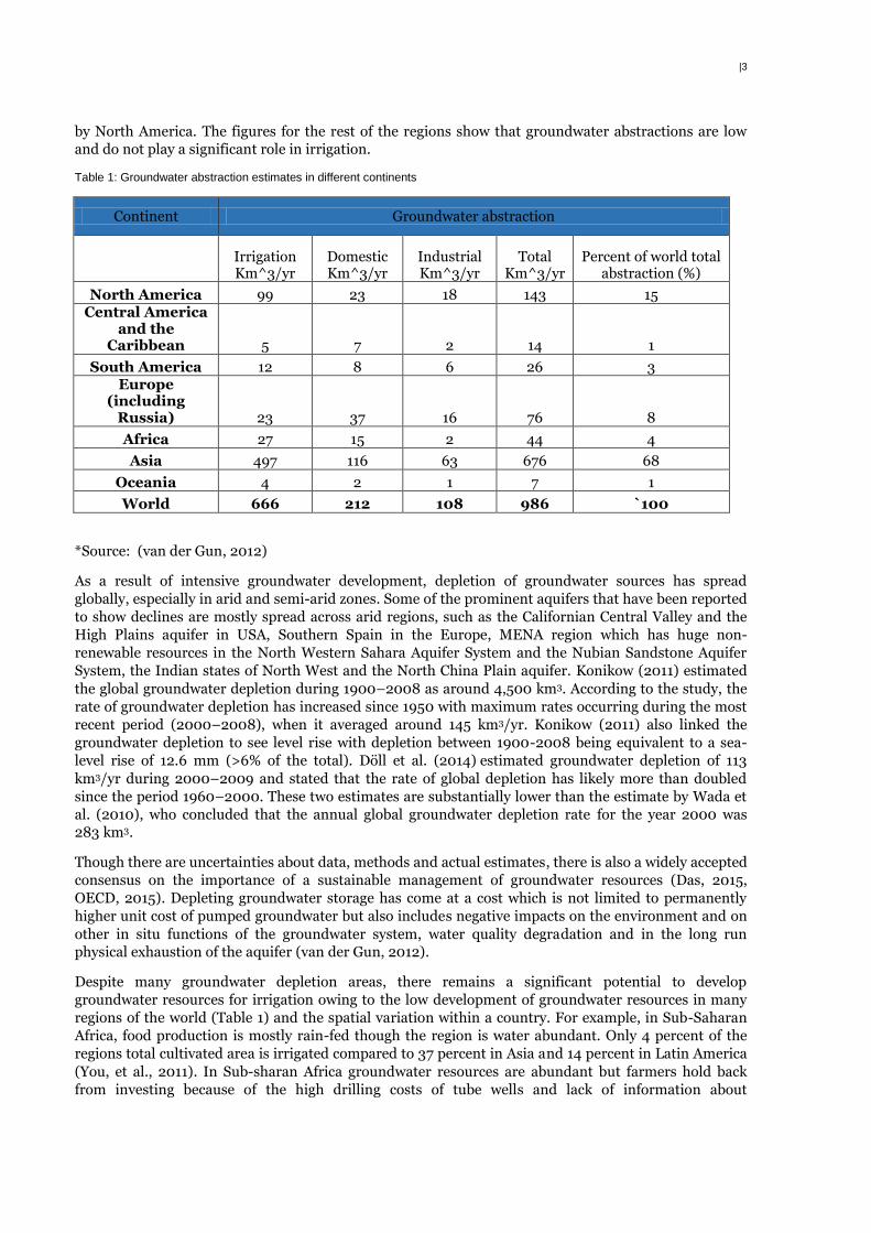
Ringler, & Cai, 2007). Table 1 gives estimates of groundwater abstraction for the year 2010 in different

world regions as reported in the United Nations World Water Assessment Program (van der Gun, 2012)

from multiple sources (IGRAC, AQUASTAT, EUROSTAT). Two-thirds of the groundwater abstraction

takes place in Asia, with India, China, Pakistan, Iran and Bangladesh as the major consumers followed

|3

by North America. The figures for the rest of the regions show that groundwater abstractions are low

and do not play a significant role in irrigation.

Table 1: Groundwater abstraction estimates in different continents

Continent Groundwater abstraction

Irrigation Km^3/yr

Domestic Km^3/yr

Industrial Km^3/yr

Total Km^3/yr

Percent of world total abstraction (%)

North America 99 23 18 143 15 Central America

and the Caribbean 5 7 2 14 1

South America 12 8 6 26 3 Europe

(including Russia) 23 37 16 76 8

Africa 27 15 2 44 4

Asia 497 116 63 676 68

Oceania 4 2 1 7 1

World 666 212 108 986 `100

*Source: (van der Gun, 2012)

As a result of intensive groundwater development, depletion of groundwater sources has spread

globally, especially in arid and semi-arid zones. Some of the prominent aquifers that have been reported

to show declines are mostly spread across arid regions, such as the Californian Central Valley and the

High Plains aquifer in USA, Southern Spain in the Europe, MENA region which has huge non-

renewable resources in the North Western Sahara Aquifer System and the Nubian Sandstone Aquifer

System, the Indian states of North West and the North China Plain aquifer. Konikow (2011) estimated

the global groundwater depletion during 1900–2008 as around 4,500 km3. According to the study, the

rate of groundwater depletion has increased since 1950 with maximum rates occurring during the most

recent period (2000–2008), when it averaged around 145 km3/yr. Konikow (2011) also linked the

groundwater depletion to see level rise with depletion between 1900-2008 being equivalent to a sea-

level rise of 12.6 mm (>6% of the total). Döll et al. (2014) estimated groundwater depletion of 113

km3/yr during 2000–2009 and stated that the rate of global depletion has likely more than doubled

since the period 1960–2000. These two estimates are substantially lower than the estimate by Wada et

al. (2010), who concluded that the annual global groundwater depletion rate for the year 2000 was

283 km3.

Though there are uncertainties about data, methods and actual estimates, there is also a widely accepted

consensus on the importance of a sustainable management of groundwater resources (Das, 2015,

OECD, 2015). Depleting groundwater storage has come at a cost which is not limited to permanently

higher unit cost of pumped groundwater but also includes negative impacts on the environment and on

other in situ functions of the groundwater system, water quality degradation and in the long run

physical exhaustion of the aquifer (van der Gun, 2012).

Despite many groundwater depletion areas, there remains a significant potential to develop

groundwater resources for irrigation owing to the low development of groundwater resources in many

regions of the world (Table 1) and the spatial variation within a country. For example, in Sub-Saharan

Africa, food production is mostly rain-fed though the region is water abundant. Only 4 percent of the

regions total cultivated area is irrigated compared to 37 percent in Asia and 14 percent in Latin America

(You, et al., 2011). In Sub-sharan Africa groundwater resources are abundant but farmers hold back

from investing because of the high drilling costs of tube wells and lack of information about

|4

groundwater availability. With the introduction of low cost technology, an irrigation potential estimated

at 42.5 million ha could be achieved (Kadigi et al., 2012). Even in India which has the highest

groundwater abstractions in the world there remains a disparity between the north western and the

eastern states. Only 31 per cent of the known groundwater potential is being developed in the eastern

states though they account for more than 55 per cent of India's net irrigated area (Srivastava et al.

2013). Thus, there is a prospective to tap the potential groundwater resources and to develop them

sustainably. This will be an adaptation measure against increasing events of droughts to which they can

provide buffer in areas where surface irrigation is practiced and offer other benefits of reliability and

higher economical returns.

1.3 Benefit cost ratio

Even though groundwater abstraction is limited by the availability of water, the implementation of

groundwater pumping systems by farmers will ultimately depend on its financial viability (Robinson,

2002). Implementation of groundwater irrigation is only cost efficient when the benefits of increased

agricultural production outweigh the construction, operation and maintenance costs of it. Cost and

benefits associated with groundwater irrigation can differ substantially for different places depending

on local and regional conditions. To assess the applicability of a measure based on cost efficiency,

benefit cost ratio calculation is usually used. For this, cost of groundwater abstraction and its benefits

are needed to be expressed in monetary terms.

1.3.1 Groundwater abstraction cost

The growth in groundwater abstraction as mentioned before has been promoted by governments

providing subsidized energy as in India (Monari, 2002) , Mexico (Scott, 2013b), Bangladesh (Mujeri et

al., 2012) as well as technological development resulting in proliferation of low cost pumps such as

treadle pumps, submersible pumps for deep bore holes and low cost well drilling techniques such as

manual drilling. This increased exploitation over the last century in many parts of the world (such as

India, China, and USA) has led to groundwater depletion leading in return to an increase in costs of

abstraction as the energy required to lift water increases with depth (Bartolino & Cunningham, 2003).

Though low cost technologies for groundwater development exist now, the cost of groundwater well

development and abstraction still act as deterrent in Sub-Saharan Africa where costs are high compared

to India and China, due to the lack of local manufacturers and competition, high excise duty on

imported drilling equipment, and insufficient use of low cost technologies (Foster et al., 2006). Also,

deep groundwater tables and groundwater depletion which increases the cost of groundwater

development acts as a limiting factor for small scale farmers who cannot afford large investments for

water abstraction (Gandhi & Namboodiri, 2009, Sharifa & Ashok, 2011).

Groundwater abstraction costs depend on size of irrigated area, choice of equipment, hydrogeology,

water table depth, fuel prices, installation costs and maintenance costs for the system. The cost per m3

of pumping groundwater depends primarily on pumping depth, energy source (electricity, diesel, solar),

and the current price of energy, whereas costs per hectare for groundwater varies also with the volume

of groundwater used during the season (Wichelns, 2010). Groundwater abstraction cost is generally

divided into two parts: capital costs and operational costs. Capital costs include well drilling, installation

and pump costs whereas operation costs include fuel prices, maintenance and repair. There have been

studies on local and regional scale to determine cost of groundwater abstractions (Robinson, 2002,

Chandrkanth, 2005, Naryanamoorthy, 2015, Kumar et al., 2014) but none on the global scale which this

study aims to determine.

Operational costs contribute the main part of the cost over the life cycle of pumps and accounts for more

than 80 % of total cost over the life time (Grundfos, 2004). Thus, the one main factor that determines

the abstraction cost is the energy source and its price. The pumps used for groundwater abstraction can

be powered by electricity, diesel or solar energy but at present high initial costs of solar pumps prohibit

its wide use despite having very low operational costs relative to the other two. Thus, accessibility and

prices of electricity and diesel at a location dominantly determine what kind of pump is used. With

groundwater irrigation contributing to 43 % of total irrigation (Siebert et al., 2010), energy prices can

have a potential effect on agriculture in terms of groundwater abstraction, crop choices of the farmer

|5

and food prices. South Asia is the world’s largest user of groundwater and uses energy worth US$ 3.78

billion per year to pump approximately 210 km3 of water for irrigation (Shah et al., 2004). Thus, owing

to the importance of energy prices in groundwater abstraction, many countries (India, Mexico, and

Bangladesh) decided to provide subsidies to promote groundwater use. This is one of the reasons for the

massive growth in groundwater irrigation in these countries which on the one side led to increase in

agricultural production but over the long term have led to groundwater depletion due to over-

abstraction.

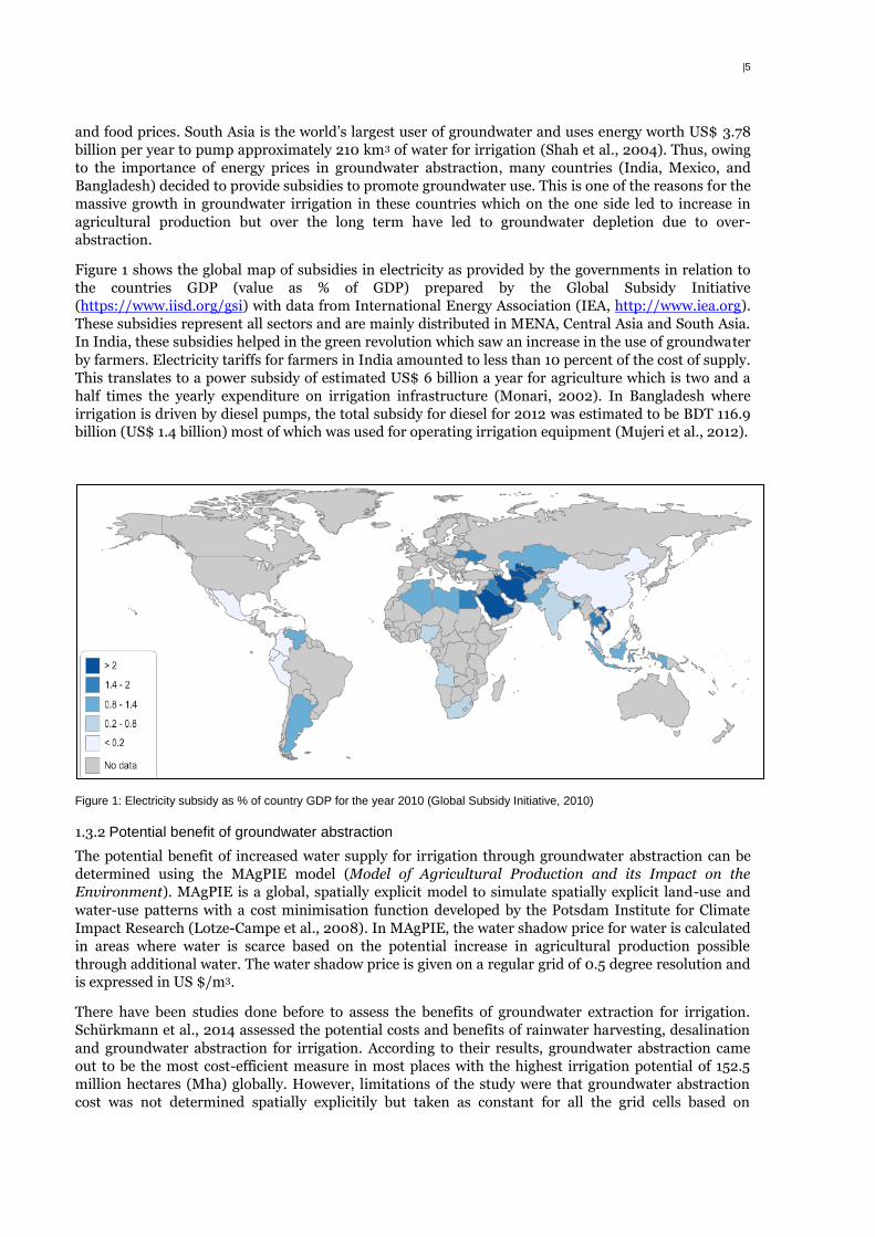
Figure 1 shows the global map of subsidies in electricity as provided by the governments in relation to

the countries GDP (value as % of GDP) prepared by the Global Subsidy Initiative

(https://www.iisd.org/gsi) with data from International Energy Association (IEA, http://www.iea.org).

These subsidies represent all sectors and are mainly distributed in MENA, Central Asia and South Asia.

In India, these subsidies helped in the green revolution which saw an increase in the use of groundwater

by farmers. Electricity tariffs for farmers in India amounted to less than 10 percent of the cost of supply.

This translates to a power subsidy of estimated US$ 6 billion a year for agriculture which is two and a

half times the yearly expenditure on irrigation infrastructure (Monari, 2002). In Bangladesh where

irrigation is driven by diesel pumps, the total subsidy for diesel for 2012 was estimated to be BDT 116.9

billion (US$ 1.4 billion) most of which was used for operating irrigation equipment (Mujeri et al., 2012).

Figure 1: Electricity subsidy as % of country GDP for the year 2010 (Global Subsidy Initiative, 2010)

1.3.2 Potential benefit of groundwater abstraction

The potential benefit of increased water supply for irrigation through groundwater abstraction can be

determined using the MAgPIE model (Model of Agricultural Production and its Impact on the

Environment). MAgPIE is a global, spatially explicit model to simulate spatially explicit land-use and

water-use patterns with a cost minimisation function developed by the Potsdam Institute for Climate

Impact Research (Lotze-Campe et al., 2008). In MAgPIE, the water shadow price for water is calculated

in areas where water is scarce based on the potential increase in agricultural production possible

through additional water. The water shadow price is given on a regular grid of 0.5 degree resolution and

is expressed in US $/m3.

There have been studies done before to assess the benefits of groundwater extraction for irrigation.

Schürkmann et al., 2014 assessed the potential costs and benefits of rainwater harvesting, desalination

and groundwater abstraction for irrigation. According to their results, groundwater abstraction came

out to be the most cost-efficient measure in most places with the highest irrigation potential of 152.5

million hectares (Mha) globally. However, limitations of the study were that groundwater abstraction

cost was not determined spatially explicitily but taken as constant for all the grid cells based on

|6

literature, the water shadow prices were determined only for areas with already existing irrigation

infrastrucuture which excluded the analysis on areas where irrigation could be expanded and finally, no

consideration was given to areas where groundwater is already overexploited. Other than that, Xie et al.

(2014) in their study estimated the small-holder irrigation potential in Sub-Saharan Africa using cost-

benefit analysis with irrigation and production costs for motor pumps, treadle pumps, communal river

diversion, and small reservoirs. Their results indicated a large potential for the expansion of smallholder

irrigation in Sub-Saharan Africa with 30 million ha for motor pumps, followed by 24 million ha for

treadle pumps, 22 million ha for small reservoirs and 20 million ha for communal river diversions. In

this case also, irrigation costs (pumping costs) in $/ha-yr were kept constant for all locations based on

literature and survey data.

1.4 Aim

This study aims to assess the benefit cost ratio of groundwater abstraction for irrigation by combining

spatially explicit groundwater abstraction costs in US $/m3 with the water shadow price from the

MAgPIE model globally on a regular grid of 0.5 degree resolution. This study overcomes the limitation

of previous studies by determining spatially explicit groundwater abstraction costs, determining water

shadow prices for all crop land area and determining areas of groundwater depeltion to exlude them

from the analysis.

Thus, this study is to the authors best knowledge, the first attempt to estimate spatially explicit

groundwater abstraction costs on global scale to assess benefit cost ratio of groundwater abstraction for

irrigation which can be used for further detailed local studies to increase agricultural production thus

achieving food security.

2. Theoretical and practical background

2.1 Groundwater recharge

Groundwater recharge is the amount of surface water which reaches the permanent water table either

by direct contact in the riparian zone or by downward percolation through the unsaturated zone

(Hiscock & Bense, 2014). Recharge forms the long term upper limit of sustainable water abstraction

from the aquifer. Recharge could take place naturally via precipitation, losing river (river recharges

groundwater), lakes, or could be done artificially with infiltration, deep well injection, irrigation, etc.

Recharge is a major component of the ground-water system and has important implications for shallow

ground-water quantity and quality. Recharge may be categorized as diffuse or focused. Diffuse recharge

refers to that which occurs over large areas as water from precipitation infiltrates and percolates

through the unsaturated zone to the water table. Focused recharge refers to water moving downward to

an aquifer from a surface-water body, such as a lake, stream, or canal (Nolan et al., 2007). Humid

regions are characterised with diffuse recharge and gaining streams whereas in arid and semi-arid

regions focussed recharge dominates with losing streams. Size of aquifers and climatic conditions affect

the recharge rates with the renewal period ranging from days and weeks in karstic zones to years or

thousands of years in large sedimentary basins. Regions where present day recharge is very low (such as

in arid and hyper-arid regions) the groundwater resources are considered non-renewable (UNESCO-

IHP, 2009).

Recharge commonly is estimated at the watershed scale using simple water-budget methods or numerical ground-water flow models (Nolan et al., 2007). Recharge estimates with site-specific data are determined using methods such as ground-water levels using lysimeters, tracers, groundwater level, and hydrograph analyses, each having its advantages and disadvantages (Hiscock & Bense, 2014). Usually a combination of models and site specific observations are used to get an overall picture of groundwater recharge in the area as recharge can vary substantially with variations in topography, soil and climatic conditions.

Determining groundwater recharge on global scale is a difficult task considering the complexity

involved in the variables influencing recharge and lack of consistent data on global scale. Döll & Fiedler

|7

(2008) calculated the long term average diffuse groundwater recharge for the period 1961–1990 with

the global hydrological model WaterGAP (Alcamo, et al., 2003) with a spatial resolution of 0.5° × 0.5°.

They calibrated the model against river discharge observations as it is linked to the baseflow from

groundwater. Döll et al. (2014) improved the above approach in a study estimating groundwater

depletion on global scale in which groundwater recharge consisted of three parts: diffuse groundwater

recharge from rain, focused recharge surface water bodies which is important in arid and semi arid

regions and return flow from agriculture. Wada et al. (2010) used the global hydrological model PCR-

GLOBWB to estimate global groundwater recharge for a spatial resolution of 0.5° × 0.5° globally for the

period 1958-2001. They didn’t explicitly include recharge from streams but mentioned that such effects

may be implicitly included when calibrating soil characteristics to reproduce observed low flow

properties. They compared their estimates to groundwater recharge from Döll & Fiedler (2008) and

found very similar patterns with their estimated total groundwater recharge, 15.2 · 103 km3 a−1 higher

than that of Döll and Fiedler (2008) which was 12.7 · 103 km3 a−1.

2.2 Saline groundwater

Groundwater quality is important considering it is abstracted for human consumptive use, irrigation,

industrial processes as well as playing an important part in ecosystem services. Though the quality of

groundwater is generally high and less prone to pollution as compared to surface water, there have been

some quality issues notably salinity, arsenic content and organic pollutants owing to natural geology

and anthropogenic reasons. Irrigation water suitability based on salinity level considering its effects on

crop yield is measured by salinity hazard and sodium hazard.

Salinity hazard is the presence of salt in irrigation water which can decrease the plant’s water

availability causing plant stress, which is dependent on soil type, plant species and salinity level.

Sodium hazard is the presence of high sodium content compared to magnesium and calcium in soils

that causes breakdown of soil aggregates, resulting in reduction in permeability and infiltration of

water. Generally a combination of salinity hazard and sodium hazard is taken into account to determine

water suitability for irrigation (Hiscock & Bense, 2014). Salinity not only decreases the agricultural

production of most crops, but also effects soil physicochemical properties and the ecological balance of

the area (Shrivastava & Kumar, 2015). Major soil and water salinity problems have been reported in

large irrigation schemes in China, India, Argentina, Sudan and many countries in Central Asia. Globally,

34 million ha (11 percent of the irrigated area) are estimated to be affected by some degree of salinity

(Mateo-Sagasta & Burke, 2010).

A report by the International Groundwater Resource Assessment Centre (IGRAC) on salinity of

groundwater (Weert et al., 2009) puts the origin of saline groundwater under four categories; marine

origin, terrestrial origin with natural factors, terrestrial origin with anthropogenic factors and mixed

origin. Irrigation with high salt content, disposal of waste water and abstraction causing sea water

intrusion are attributed to anthropogenic factors whereas dissolution of subsurface mineral salts,

evaporation in shallow water tables in arid zones, and old sea fossil water are some of the natural

factors for saline groundwater.

The limit of salt in irrigation water is determined by a combination of salinity hazard and sodium

hazard which depends on soil type, crop tolerance, management practices and climatic conditions. In

addition, there are some general guidelines available which could be used to determine whether water is

suitable for irrigation or not. According to Hiscock & Bense (2014), 1-2 g/l of salt content can have

adverese effects on many crops whereas 2-5 g/l could be used only for salt tolerant crops with

permeable soils and good management practices. According to the FAO manual on irrigation water

management (Brouwer et al., 1985), water with more than 2g/l of salt concentration has high risk and is

not advised to use unless consulted with specialists. A content of greater than 3 ds/m (approximately

2g/l) is considered severe and to be used only with good drainage and tolerant plants (Bauder et al.,

2014).

|8

2.3 Groundwater depletion

Groundwater discharge in excess of recharge provides an estimate of the amount of groundwater depletion. Groundwater discharge takes place primarily through two ways: natural discharge also called baseflow to surface water bodies and human abstraction notably through well pumping. Groundwater abstraction by pumping plays an important part in achieving water security of humans whereas natural discharge is very important for ecosystems in keeping the water level and flow into rivers, lakes and wetlands termed as groundwater dependent ecosystems by Murray et al. (2003). The natural discharge becomes quite important during the drier months when there is little direct water from rainfall in surface water bodies. Without human influence over a long period of time, groundwater recharge and discharge rates reaches an equilibrium which gives rise to a natural water table. The case where abstractions exists but are less than recharge rates would lead to reduced streamflow, but will not lead to ongoing depletion of groundwater reserves (Wada et al., 2010).

Some of the negative effects of groundwater depletion includes drying up of wells, reduction of water in streams and lakes affecting ecosystems, deterioration of water quality, increased pumping costs, land subsidence and sea water intrusion (Alley et al., 1999). Overexploitation of groundwater resources especially in areas where it is used for irrigation such as high plains aquifers in USA, India, China, and Mexico have resulted in groundwater depletion (Shah et al., 2000).

2.4 Irrigation-induced problems

Apart from the fact that excessive groundwater pumping for irrigation can lead to groundwater

depletion, there are other problems of inefficient or excessive irrigation. Some of these problems are:

salinity, water logging, soil erosion and sedimentation, and water pollution (Umali, 1993). One of the

main concerns is the irrigation induced salinity which is exacerbated by excessive irrigation.

Salt-induced land degradation is common in arid and semi-arid regions where rainfall is too low to

maintain a regular percolation of rainwater through the soil and irrigation is practiced without a natural

or artificial drainage system (Qadir, et al., 2014,(Singh, 2015). This could be caused by increasing

groundwater levels resulting from excess perenial irrigation with poor drainage bringing salts to upper

layer of soil or could be induced by using poor quality of groundwater for irrigation (Kijne et al., 1998).

Datta and Jong, 2002 calculated the damaged caused by salinity in Indian state of Haryana over a

period of 30 years and concluded that overall loss from 500,000 ha of waterlogged saline land in

Haryana is about US$ 35 million per year. Qadir et al., 2014 concluded that with a wide range of

revenue losses associated with soil salinization may result in 15-69% losses depending on the crop

grown, land degradation type and its intensity, irrigation water quality, provision and capacity of

drainage system, and water distribution and on-farm soil and water management. In addition, he

concluded that there are other cost implications such as employment losses, increase in human and

animal health problems and treatment costs, losses in property values of farms with degraded land, and

the social cost of farm businesses.

2.5 Groundwater aquifer types

The type of aquifer and its properties determine the ease of access to groundwater, its quality, recharge rates and yield which are very important and limiting factors in groundwater abstraction. In a report by UNESCO/BGR (Vrba & Richts, 2015), aquifer were divide into 7 types with three most important for abstraction are: Local and shallow and shallow aquifer, major groundwater basins and complex hydrogeological structures.

Local and shallow aquifers are minor but locally productive and are limited to the alteration zone of the

bedrock and overlying shallow layers. At the same time they are highly vulnerable to flood, storms and

droughts in arid and semi-arid regions. Aquifers in major groundwater basins are extensive and

productive containing large amount of groundwater and are areas where most of the groundwater

abstraction on large scale takes place. Aquifers in complex hydrogeological structures include

|9

groundwater flow systems in fissures and fractures. In such aquifers productive aquifers can occur in

close proximity to non-productive aquifers (Vrba & Richts, 2015).

Major groundwater basins such as the Ogallala Aquifer of the Great Plains in the USA, the Northern

China plain aquifer, and the Indus basin aquifer in Pakistan have been the areas of extensive irrigation

from groundwater leading to groundwater depletion, but showing their potential. Aquifers in complex

hydrogeological structures have also been exploited for irrigation notably in Indian Deccan areas,

whereas local and shallow aquifers potential is still not that developed for irrigation owing to variable

yields, and are largely located in Sub-Saharan Africa. Thus, major and complex aquifers present good

opportunities for exploitation, whereas the potential of shallow aquifers is local and has to be tested for

yields for irrigation use as it can be limited by that.

2.6 Groundwater abstraction cost

The costs of groundwater abstraction consist of the sum of full supply cost (or cost paid by users) and

full economy costs. Full supply costs are the costs associated with groundwater abstraction without

considering the externalities of abstraction or the alternative use of water (opportunity cost) whereas

full economy costs also include opportunity cost and the costs of negative externalities (OECD, 2010,

Das, 2015). Full economy costs are more of a theoretical construct which is difficult to determine as it is

difficult to directly value external and opportunity costs.

The full supply costs consist of two components: capital and operational costs. Capital costs includes the

costs for the installation of groundwater abstraction systems, including the price for pumps, well

drilling and installation, whereas operational costs consist of fuel prices, repair and maintenance. In

addition to capital and operational costs, full economy costs also have the opportunity and external

costs. Opportunity costs address the cost of one consumer depriving another of the use of the water

(public water supply, irrigation for high value crop) if that other use has a higher value for the water, i.e.

the foregone value of alternative users (present and future) (OECD, 2010). External cost is the in-situ

value which refers to services rendered by standing groundwater or cost associated with externalities if

water is abstracted like subsidence, recharge to streams, or protection against sea water intrusion

(Strand, 2010).

While the first part of the full supply cost which includes capital and operational costs is relatively easy

to measure through determination of capital costs incurred and fuel prices charged, the second part,

valuing external and opportunity costs is complex as it covers goods and services that are not usually

marketed, such as indirect use (e.g. wetlands or pollution), or barrier to salt water intrusion (OECD,

2010). Thus the first part that determines the cost of groundwater abstraction for users is also termed as

cost paid by users by Das (2015). For the above mentioned reasons, studies intending to derive the costs

of groundwater abstraction for irrigation (Robinson, 2002, Chandrkanth, 2005, Naryanamoorthy,

2015) are limited to the first part which includes capital and operation costs incurred by the farmer.

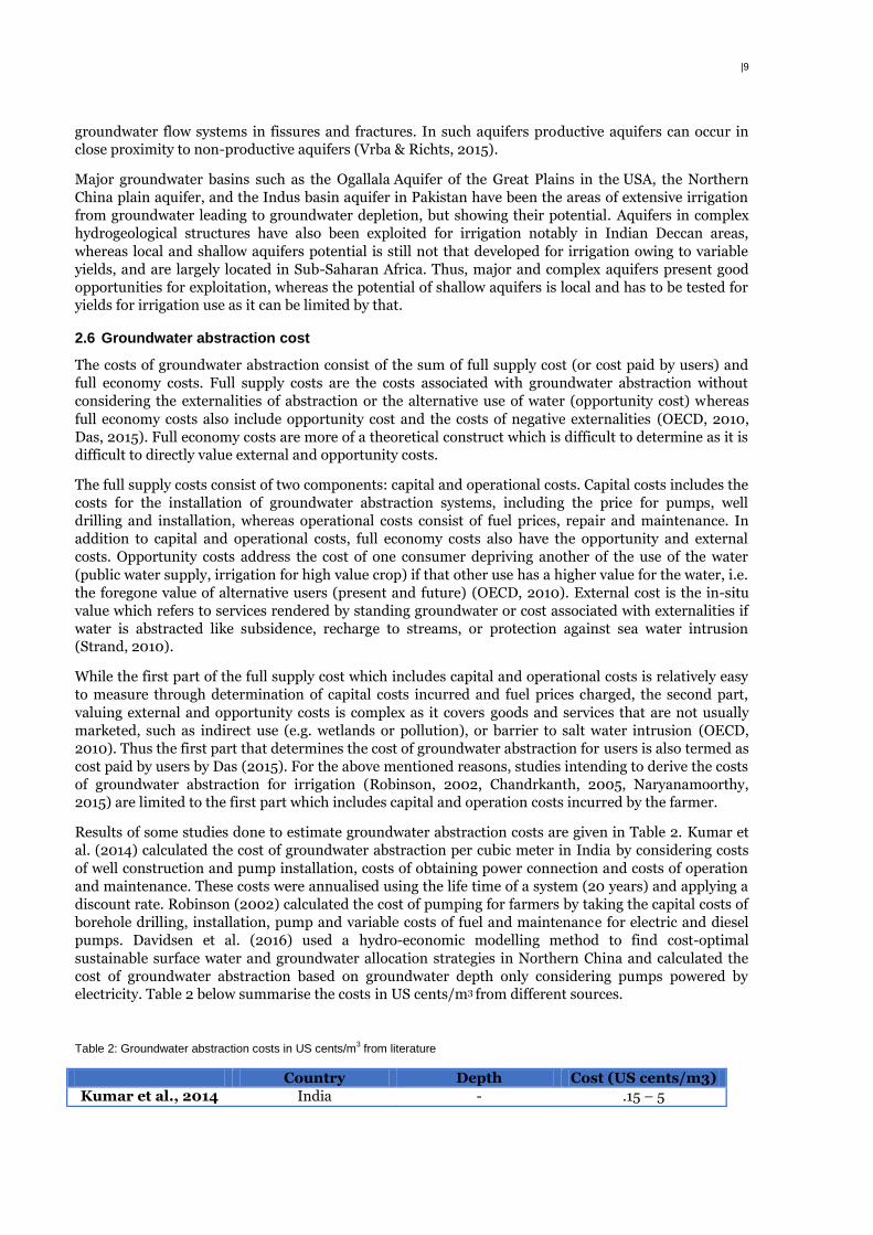
Results of some studies done to estimate groundwater abstraction costs are given in Table 2. Kumar et

al. (2014) calculated the cost of groundwater abstraction per cubic meter in India by considering costs

of well construction and pump installation, costs of obtaining power connection and costs of operation

and maintenance. These costs were annualised using the life time of a system (20 years) and applying a

discount rate. Robinson (2002) calculated the cost of pumping for farmers by taking the capital costs of

borehole drilling, installation, pump and variable costs of fuel and maintenance for electric and diesel

pumps. Davidsen et al. (2016) used a hydro-economic modelling method to find cost-optimal

sustainable surface water and groundwater allocation strategies in Northern China and calculated the

cost of groundwater abstraction based on groundwater depth only considering pumps powered by

electricity. Table 2 below summarise the costs in US cents/m3 from different sources.

Table 2: Groundwater abstraction costs in US cents/m3 from literature

Country Depth Cost (US cents/m3)

Kumar et al., 2014 India - .15 – 5

|10

Robinson, 2002 Australia 140 m 5 - 6

Davidsen et al., 2016

China 200 m 12

2.1.1 Capital costs

In surface irrigation, water is delivered through canals with gravity flows whereas in case of

groundwater, water needs to be pumped. The primary function of a pump is to transfer energy from a

power source to a fluid, and as a result to create flow, lift, or greater pressure on the fluid (Haman,

2014). Pumping can be done with manual devices like treadle pumps, rope pumps or with fuel powered

mechanised motor pumps which could be powered by electricity, diesel, solar or wind power. Manual

pumping is limited to areas with shallow groundwater. There are large varieties of pumps available for

groundwater abstraction for different purposes and areas in the market. Different factors have to be

taken into account while selecting a pump, such as properties of the process liquid, flow rate and

pressure, power source availability and certain specific requirements in connection with the pump.

2.1.1.1 Pump types based on energy source

The pumps used at present are mainly powered by diesel and electricity, and increasingly with solar

energy considering the inclination towards renewable energy with governments more or less promoting

and providing subsidies for solar pumps. The factor that drives the use of different pumps is the initial

capital cost, access to energy source and government policies and subsidies.

There are many advantages of using electricity driven pumps over diesel pumps. The running costs of an

electrically powered pumping system is less than a diesel powered system because of lower power and

maintenance costs (Robinson, 2002). Typical pump efficiencies for electrical pumps range between 70

to 80 per cent, whereas diesel pumps have an efficiency of just 30 to 40 per cent. Other advantages of

electric pumps include lower maintenance requirements, less environmental impacts, and more easily

implemented pump controls. Around 90% of a life time cost of pumps is operational (Grundfos, 2004),

thus the use of an electric pump is much more efficient and cost saving.

Despite all the advantages, the factors that still motivate and in many parts of the world lead to a

domination of diesel power pumps are the high cost of power line extension for electricity connection,

low installation costs and unreliable electric power supplies which is a major concern in developing

countries like India and Pakistan. In a study in Pakistan, Qureshi et al. (2003) found that after 1991 the

installation of diesel powered pumps increased due to an unreliable infrastructure with high risk of

power cuts and high capital cost of the installation of electricity connections. Bangladesh’s agricultural

sector depends heavily on energy intensive irrigation with nearly 87 percent of the irrigation equipment

running on diesel, accounting for nearly 71 percent of the area under mechanized irrigation (Mujeriet et

al., 2012).

On the contrary, in India the number of electrified pump-sets has increased to over 16 million in 2009

from 12 million in 1999 with 85% of the total water pumped through electric pumps due to de-

regulation of diesel prices and reduced diesel subsidy to the agricultural sector (Niti Aayog, 2015). The

principal energy source for pumping groundwater in Mexico is also electricity, limiting diesel engines to

low lifts from open water sources (Scott & Shah, 2004). Power line extension is expensive so therefore if

power connection costs are relatively low compared to the total capital cost of the pumping system, an

electrically powered pumping system is more cost efficient than a diesel powered system to pump

groundwater (Robinson, 2002).

Solar water pumps are increasing in prominence but still contribute only to a very small percentage due

to the many implementation barriers such as high upfront capital cost, lack of finance mechanisms, low

awareness and support needed, etc. (Pullenkav, 2013). Erratic grid supply and high cost of diesel

pumping continue to remain problematic areas for the farmers which encourage the use of solar

powered pumps. However, the upfront cost of a solar pump is about ten times of a conventional pump

and hence it requires capital subsidy and financing support (KPMG, 2014).

|11

2.1.1.2 Pump types based on operating principle

Pumps are generally classified based on their operating principle, which means by the way they add

energy to a fluid. In general, pumps are classified into two main types:

Positive displacement pumps

Centrifugal pumps (or roto-dynamic)

Positive displacement pumps work by pressurising and moving the fluid. They work by expanding and

then compressing a cavity, space, or moveable boundary within the pump. In most cases, these pumps

actually capture the liquid and physically transport it through the pump to the discharge nozzle. In

contrast, centrifugal pumps speed up the fluid and convert this kinetic energy to pressure, thus

generating pressure by accelerating, and then decelerating the movement of the fluid through the pump

(Bachus & Custodio, 2003, Hyudraulic Institute and ITP, 2006). Within these classifications many

different subcategories can be found. Positive displacement pumps are categorised into: piston, screw,

sliding vane, and rotary lobe types whereas centrifugal pumps are categorised into axial (propeller),

mixed-flow, and radial types (Hyudraulic Institute and ITP, 2006).

In agriculture, mostly centrifugal pumps are used (Haman, 2014, Koegelenberg, 2004) as displacement

pumps are not suitable for pumping the large amounts of water required but are generally for

application such as with viscous liquids, precise metering, and dosification, conditions where pressures

are high with little flow (Bachus & Custodio, 2003). Centrifugal pumps are more common also because

they are simple and safe to operate, require minimal maintenance, and have characteristically long

operating lives (Hyudraulic Institute and ITP, 2006).

The two most common types of centrifugal pumps used in the irrigation are: End-suction centrifugal

pumps and Submersible pumps. Both of them could be single or multistage. End-suction pumps are the

most commonly used centrifugal pumps, and it is the most basic centrifugal pump. These are usually

equipped with radial flow impellers but mixed flow impellers are also used (Koegelenberg, 2004). The

pump could be single or multistage but mostly they are single stage pumps. The pump is “close-

coupled” to an electric motor, that is, the pump is connected directly onto the motors drive shaft and the

pump case is bolted to the motor so that it looks like a single unit. Some variants are also long “coupled”

where the motor is connected by a flexible coupling and has a separate bearing structure (Grundfos,

2004).

End-suction centrifugal pumps are not the best choice for drawing water from a water source that is

more than a few feet lower than the pump because of net suction positive head pressures (NPSH) which

can cause cavitations affecting pump performance. When abstracting groundwater, they must be

installed where groundwater tables are low, thus they are great for use as irrigation booster pumps as

they are designed to push water but not pull it (Stryker, n.d.). They are suitable for pumping from

shallow depths and are popular because they are cheap and portable.

Submersible centrifugal pumps are pumps that are installed completely underwater, including the

motor. Two types of borehole pumps exist: The submerged borehole pump type with a submersible

motor (Figure 2) and the deep well pump with a dry motor, which is connected to the pump by a long

shaft (Grundfos, 2004). The long shaft of the deep well pump is a drawback, so submerged borehole

type pumps are mostly used in agriculture, as the temperature of water abstracted is not high which is

one area where a dry motor is needed as to cool it down on the surface. Pump types are made to be

installed in deep and narrow boreholes and have thus a reduced diameter, which makes them longer

than other pump types. Typically the pump will be shaped like a long narrow cylinder so that it can fit

down inside of a borehole well casing (Stryker, n.d.).

Submersible borehole pumps tend to be more energy efficient because they only push the water in

comparison to end suction pumps which also need to suck in water. Mostly submersible pumps are

“multi-stage” pumps that are actually several smaller centrifugal pumps stacked on top of each other to

create higher flow, more water pressure, or a combination of both. The pump is always filled with water

so no priming is needed and they operate more quietly than above ground installations. One of the

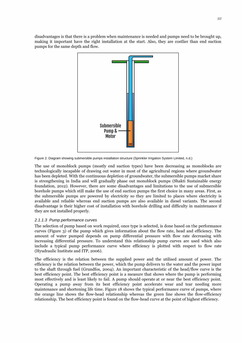
|12

disadvantages is that there is a problem when maintenance is needed and pumps need to be brought up,

making it important have the right installation at the start. Also, they are costlier than end suction

pumps for the same depth and flow.

Figure 2: Diagram showing submersible pumps installation structure (Sprinkler Irrigation System Limited, n.d.)

The use of monoblock pumps (mostly end suction types) have been decreasing as monoblocks are

technologically incapable of drawing out water in most of the agricultural regions where groundwater

has been depleted. With the continuous depletion of groundwater, the submersible pumps market share

is strengthening in India and will gradually phase out monoblock pumps (Shakti Sustainable energy

foundation, 2012). However, there are some disadvantages and limitations to the use of submersible

borehole pumps which still make the use of end suction pumps the first choice in many areas. First, as

the submersible pumps are powered by electricity so they are limited to places where electricity is

available and reliable whereas end suction pumps are also available in diesel variants. The second

disadvantage is their higher cost of installation with borehole drilling and difficulty in maintenance if

they are not installed properly.

2.1.1.3 Pump performance curves

The selection of pump based on work required, once type is selected, is done based on the performance

curves (Figure 3) of the pump which gives information about the flow rate, head and efficiency. The

amount of water pumped depends on pump differential pressure with flow rate decreasing with

increasing differential pressure. To understand this relationship pump curves are used which also

include a typical pump performance curve where efficiency is plotted with respect to flow rate

(Hyudraulic Institute and ITP, 2006).

The efficiency is the relation between the supplied power and the utilised amount of power. The

efficiency is the relation between the power, which the pump delivers to the water and the power input

to the shaft through fuel (Grundfos, 2004). An important characteristic of the head/flow curve is the

best efficiency point. The best efficiency point is a measure that shows where the pump is performing

most effectively and is least likely to fail. A pump should operate at or near the best efficiency point.

Operating a pump away from its best efficiency point accelerate wear and tear needing more

maintenance and shortening life time. Figure 18 shows the typical performance curve of pumps, where

the orange line shows the flow-head relationship whereas the green line shows the flow-efficiency

relationship. The best efficiency point is found on the flow-head curve at the point of highest efficiency.

|13

Figure 3: Pump performance curves. The orange line represents the Flow-Head relationship and the green line represents the

Flow-Efficiency relationship (Vogel, 2013).

2.1.1.4 Pump efficiency (p , m )

The efficiency of an electric motor is the ratio of supplied electrical power to converted mechanical

power, known as motor efficiency ( m ). The main energy loss occurs when this mechanical power

supplied by the motor is converted to hydraulic energy (flow, velocity, pressure) by means of the

pumping system, which is reported in terms of pump efficiency (p ).

Through the importance of maintaining high efficiency is well known, pump operating efficiencies

remain low due to lack of awareness among farmers, low maintenance and repair, and certain

governmental policies like subsidies. For example, in India the end-use efficiency of agricultural pump

sets is dismally low due to heavily subsidised agricultural power which leaves farmers with little

incentive for efficient use of electricity, which is reflected in the purchase preference for cheap but

inefficient pumps (Singh, 2009). A study of a sample of pump sets in a Bangalore rural district in

Karnataka state, India, found that 91 per cent of the pumps were operating at the efficiency of less than

30 per cent (Oza, 2007). Field testing programs in Colorado, Wyoming, Nebraska, Texas, Louisiana and

other states in USA have shown that the overall pumping plant efficiencies for electrically driven pumps

average 45 to 55 percent, as compared to a realistically achievable efficiency of 72 to 77 percent (Chávez,

Reich, Loftis, & Miles, 2011).

2.1.1.5 Pump operating hours (T)

The average running hours annually reported in the literature varied with 1000 hours in Europe

(Falkner, 2008), 107 to 1636 hours in South Asia (Shah et al., 2004) and over 4000 hours in Mexico

(Scott et al. , 2002). The total pumping hours depend on the water available, crop water requirements,

number of crops, growing season and climate, thus the cost per hectare could be calculated by

multiplying cost per cubic metre to the water requirement.

2.1.1.6 Pump maintenance and repair cost

Maintenance and repair costs are difficult to determine and vary with the operating conditions and

pump type. Generally, repair and maintenance costs for electric pumps are lower than for diesel pumps.

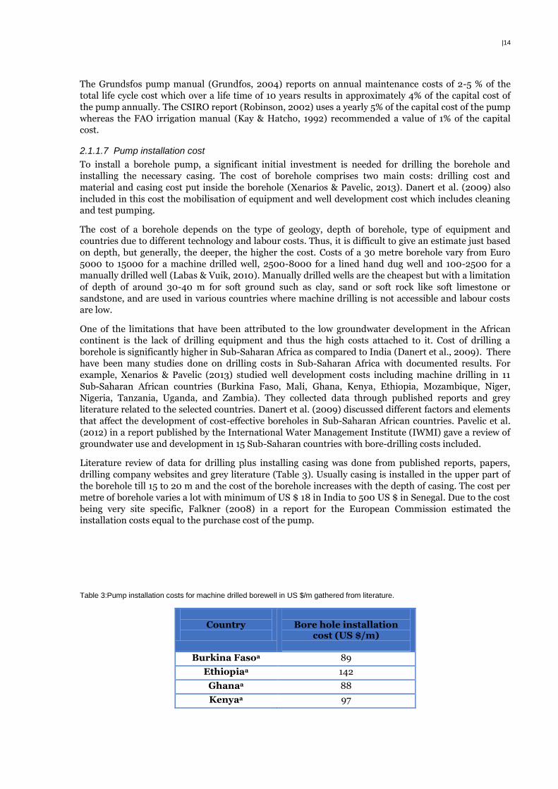
|14

The Grundsfos pump manual (Grundfos, 2004) reports on annual maintenance costs of 2-5 % of the

total life cycle cost which over a life time of 10 years results in approximately 4% of the capital cost of

the pump annually. The CSIRO report (Robinson, 2002) uses a yearly 5% of the capital cost of the pump

whereas the FAO irrigation manual (Kay & Hatcho, 1992) recommended a value of 1% of the capital

cost.

2.1.1.7 Pump installation cost

To install a borehole pump, a significant initial investment is needed for drilling the borehole and

installing the necessary casing. The cost of borehole comprises two main costs: drilling cost and

material and casing cost put inside the borehole (Xenarios & Pavelic, 2013). Danert et al. (2009) also

included in this cost the mobilisation of equipment and well development cost which includes cleaning

and test pumping.

The cost of a borehole depends on the type of geology, depth of borehole, type of equipment and

countries due to different technology and labour costs. Thus, it is difficult to give an estimate just based

on depth, but generally, the deeper, the higher the cost. Costs of a 30 metre borehole vary from Euro

5000 to 15000 for a machine drilled well, 2500-8000 for a lined hand dug well and 100-2500 for a

manually drilled well (Labas & Vuik, 2010). Manually drilled wells are the cheapest but with a limitation

of depth of around 30-40 m for soft ground such as clay, sand or soft rock like soft limestone or

sandstone, and are used in various countries where machine drilling is not accessible and labour costs

are low.

One of the limitations that have been attributed to the low groundwater development in the African

continent is the lack of drilling equipment and thus the high costs attached to it. Cost of drilling a

borehole is significantly higher in Sub-Saharan Africa as compared to India (Danert et al., 2009). There

have been many studies done on drilling costs in Sub-Saharan Africa with documented results. For

example, Xenarios & Pavelic (2013) studied well development costs including machine drilling in 11

Sub-Saharan African countries (Burkina Faso, Mali, Ghana, Kenya, Ethiopia, Mozambique, Niger,

Nigeria, Tanzania, Uganda, and Zambia). They collected data through published reports and grey

literature related to the selected countries. Danert et al. (2009) discussed different factors and elements

that affect the development of cost-effective boreholes in Sub-Saharan African countries. Pavelic et al.

(2012) in a report published by the International Water Management Institute (IWMI) gave a review of

groundwater use and development in 15 Sub-Saharan countries with bore-drilling costs included.

Literature review of data for drilling plus installing casing was done from published reports, papers,

drilling company websites and grey literature (Table 3). Usually casing is installed in the upper part of

the borehole till 15 to 20 m and the cost of the borehole increases with the depth of casing. The cost per

metre of borehole varies a lot with minimum of US $ 18 in India to 500 US $ in Senegal. Due to the cost

being very site specific, Falkner (2008) in a report for the European Commission estimated the

installation costs equal to the purchase cost of the pump.

Table 3:Pump installation costs for machine drilled borewell in US $/m gathered from literature.

Country

Bore hole installation

cost (US $/m)

Burkina Fasoa 89

Ethiopiaa 142

Ghanaa 88

Kenyaa 97

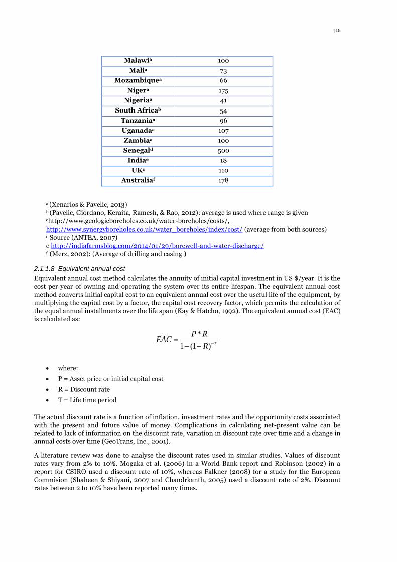
|15

Malawib 100

Malia 73

Mozambiquea 66

Nigera 175

Nigeriaa 41

South Africab 54

Tanzaniaa 96

Uganadaa 107

Zambiaa 100

Senegald 500

Indiae 18

UKc 110

Australiaf 178

a (Xenarios & Pavelic, 2013)

b (Pavelic, Giordano, Keraita, Ramesh, & Rao, 2012): average is used where range is given chttp://www.geologicboreholes.co.uk/water-boreholes/costs/,

http://www.synergyboreholes.co.uk/water_boreholes/index/cost/ (average from both sources) d Source (ANTEA, 2007)

e http://indiafarmsblog.com/2014/01/29/borewell-and-water-discharge/ f (Merz, 2002): (Average of drilling and casing )

2.1.1.8 Equivalent annual cost

Equivalent annual cost method calculates the annuity of initial capital investment in US $/year. It is the

cost per year of owning and operating the system over its entire lifespan. The equivalent annual cost

method converts initial capital cost to an equivalent annual cost over the useful life of the equipment, by

multiplying the capital cost by a factor, the capital cost recovery factor, which permits the calculation of

the equal annual installments over the life span (Kay & Hatcho, 1992). The equivalent annual cost (EAC)

is calculated as:

*

1 (1 ) T

P REAC

R

where:

P = Asset price or initial capital cost

R = Discount rate

T = Life time period

The actual discount rate is a function of inflation, investment rates and the opportunity costs associated

with the present and future value of money. Complications in calculating net-present value can be

related to lack of information on the discount rate, variation in discount rate over time and a change in

annual costs over time (GeoTrans, Inc., 2001).

A literature review was done to analyse the discount rates used in similar studies. Values of discount

rates vary from 2% to 10%. Mogaka et al. (2006) in a World Bank report and Robinson (2002) in a

report for CSIRO used a discount rate of 10%, whereas Falkner (2008) for a study for the European

Commision (Shaheen & Shiyani, 2007 and Chandrkanth, 2005) used a discount rate of 2%. Discount

rates between 2 to 10% have been reported many times.

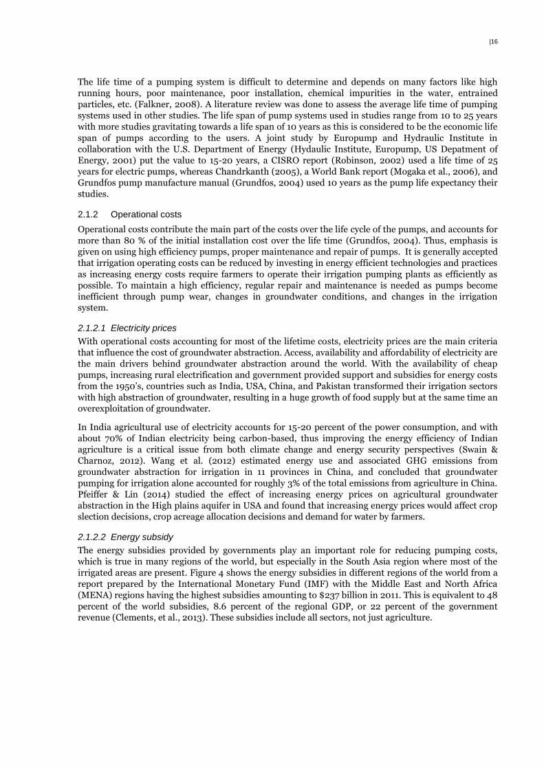
|16

The life time of a pumping system is difficult to determine and depends on many factors like high

running hours, poor maintenance, poor installation, chemical impurities in the water, entrained

particles, etc. (Falkner, 2008). A literature review was done to assess the average life time of pumping

systems used in other studies. The life span of pump systems used in studies range from 10 to 25 years

with more studies gravitating towards a life span of 10 years as this is considered to be the economic life

span of pumps according to the users. A joint study by Europump and Hydraulic Institute in

collaboration with the U.S. Department of Energy (Hydaulic Institute, Europump, US Depatment of

Energy, 2001) put the value to 15-20 years, a CISRO report (Robinson, 2002) used a life time of 25

years for electric pumps, whereas Chandrkanth (2005), a World Bank report (Mogaka et al., 2006), and

Grundfos pump manufacture manual (Grundfos, 2004) used 10 years as the pump life expectancy their

studies.

2.1.2 Operational costs

Operational costs contribute the main part of the costs over the life cycle of the pumps, and accounts for

more than 80 % of the initial installation cost over the life time (Grundfos, 2004). Thus, emphasis is

given on using high efficiency pumps, proper maintenance and repair of pumps. It is generally accepted

that irrigation operating costs can be reduced by investing in energy efficient technologies and practices

as increasing energy costs require farmers to operate their irrigation pumping plants as efficiently as

possible. To maintain a high efficiency, regular repair and maintenance is needed as pumps become

inefficient through pump wear, changes in groundwater conditions, and changes in the irrigation

system.

2.1.2.1 Electricity prices

With operational costs accounting for most of the lifetime costs, electricity prices are the main criteria

that influence the cost of groundwater abstraction. Access, availability and affordability of electricity are

the main drivers behind groundwater abstraction around the world. With the availability of cheap

pumps, increasing rural electrification and government provided support and subsidies for energy costs

from the 1950’s, countries such as India, USA, China, and Pakistan transformed their irrigation sectors

with high abstraction of groundwater, resulting in a huge growth of food supply but at the same time an

overexploitation of groundwater.

In India agricultural use of electricity accounts for 15-20 percent of the power consumption, and with

about 70% of Indian electricity being carbon-based, thus improving the energy efficiency of Indian

agriculture is a critical issue from both climate change and energy security perspectives (Swain &

Charnoz, 2012). Wang et al. (2012) estimated energy use and associated GHG emissions from

groundwater abstraction for irrigation in 11 provinces in China, and concluded that groundwater

pumping for irrigation alone accounted for roughly 3% of the total emissions from agriculture in China.

Pfeiffer & Lin (2014) studied the effect of increasing energy prices on agricultural groundwater

abstraction in the High plains aquifer in USA and found that increasing energy prices would affect crop

slection decisions, crop acreage allocation decisions and demand for water by farmers.

2.1.2.2 Energy subsidy

The energy subsidies provided by governments play an important role for reducing pumping costs,

which is true in many regions of the world, but especially in the South Asia region where most of the

irrigated areas are present. Figure 4 shows the energy subsidies in different regions of the world from a

report prepared by the International Monetary Fund (IMF) with the Middle East and North Africa

(MENA) regions having the highest subsidies amounting to $237 billion in 2011. This is equivalent to 48

percent of the world subsidies, 8.6 percent of the regional GDP, or 22 percent of the government

revenue (Clements, et al., 2013). These subsidies include all sectors, not just agriculture.

|17

Figure 4: Energy subsidies in absolute amount (US $) and as percent of GDP for the world regions and economies (Clements, et

al., 2013, Sdralevich, Sab, Zouhar, & Albertin, 2014).

For example in India, Audinet (2002) reported an average agriculture tariff of 25 paise/kWh (0.37

cents/KWh) in 1999-2000, Badiani & Jessoe (2010) reported a maximum value of 270 paise/kWh (4.05

cents/KWh) in the state of Assam but all other values were less than 200 paise/kWh (3 cents/KWh and

mostly around 100 paise/kWh (1.5 cents/KWh) for different states for year 2004. Sharma et al. (2015)

reported from Central Electricity authority data that in 2010–11 the average all India cost of per kWh of

power was INR 3.78 (5.68 cents), but the agricultural sector was only charged INR 1.15 per kWh (1.73

cents) of power.

Similarly in Mexico, electricity subsidies for pumping play a big part with agricultural prices at the

lowest and an estimated net subsidy of US $ 6 billion per year (CEE/ITESM, 2006). Electricity for

groundwater pumping is subsidized by a factor of two to four times compared to the commercial rates,

and a special ‘night-time stimulus tariff for pumping water for agricultural irrigation’ was introduced

from 2004 (Scott C. A., 2013 (b)). Night tariff of Mex$ 0.17/kWh (1 US cents/kWh) is used by Scott

(2011), which is set at half the day prices to study the energy-water nexus in Mexico, which is much

lower than 8.7 US cents/kWh used without subsidy.

Electric subsidies have helped farmers to reduce their costs in India but at the same time the quality of

supply to farmers has worsened over the years because of operational inefficiencies and high

distribution losses due to unsustainable finances of power utilities across India (Monari, 2002). As a

result, farmers get unreliable and intermittent supply, impacting water availability during critical

periods in the plant growth cycle, which leads to lower crop yields and motor burnouts affecting

incomes for farmers. This also leads to an over-abstraction of water resulting in depletion and affecting

local ecosystems depending on groundwater. Due to these reasons, removing electricity subsidies is

frequently advocated as a policy change.

2.1.2.3 Groundwater table depth

The groundwater table depth is the upper level of an underground surface in which the soil or rocks are

permanently saturated with water. The depth of the groundwater table is one of the main factors that

govern the exploitation of groundwater as with deeper water table depth, costs of abstraction become

high. There is a high variability in the availability of data on water table depth (WTD) as primary data

sources have to be observational of which there are only few and mainly concentrated in the developed

world. Modelling of the groundwater table using global models is a challenging task considering the

variability and lack of knowledge about the aquifer properties, like transmissivity, recharge rates, etc.

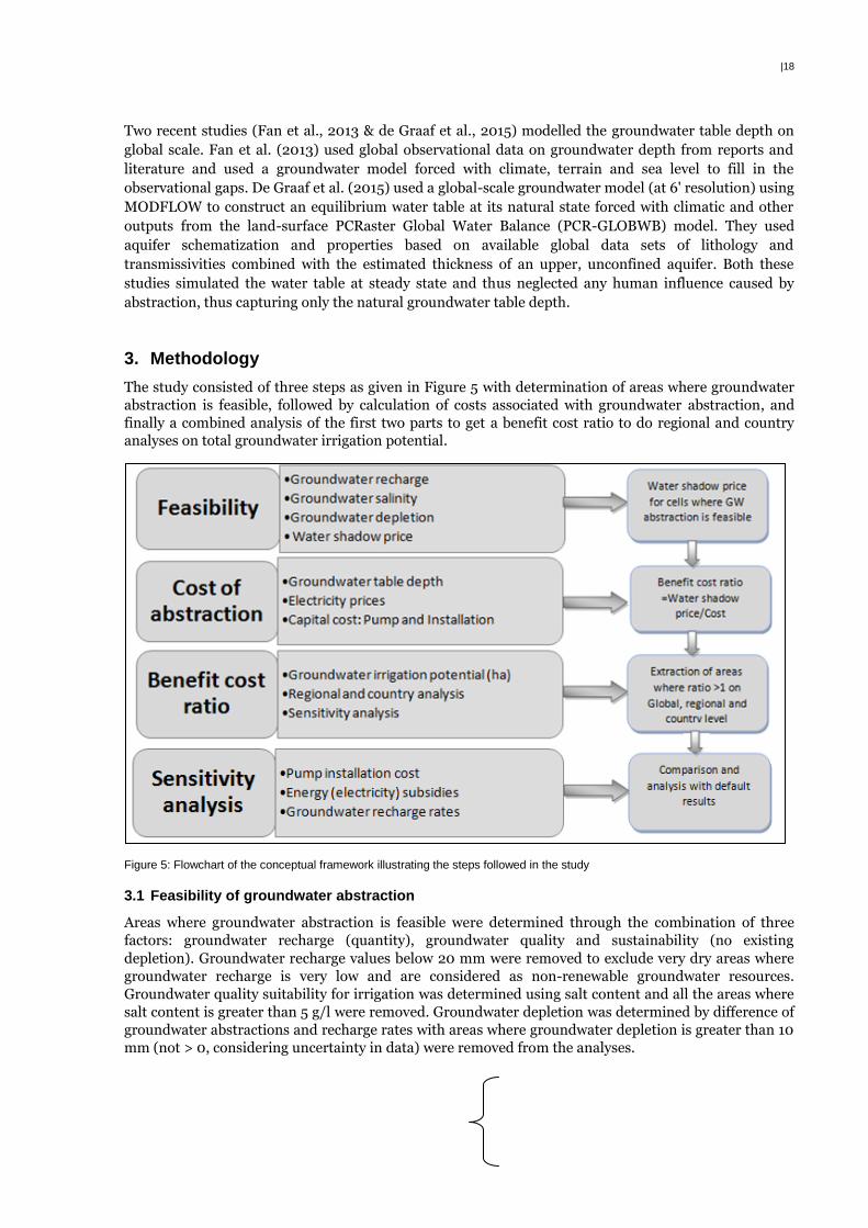
|18

Two recent studies (Fan et al., 2013 & de Graaf et al., 2015) modelled the groundwater table depth on

global scale. Fan et al. (2013) used global observational data on groundwater depth from reports and

literature and used a groundwater model forced with climate, terrain and sea level to fill in the

observational gaps. De Graaf et al. (2015) used a global-scale groundwater model (at 6' resolution) using

MODFLOW to construct an equilibrium water table at its natural state forced with climatic and other

outputs from the land-surface PCRaster Global Water Balance (PCR-GLOBWB) model. They used

aquifer schematization and properties based on available global data sets of lithology and

transmissivities combined with the estimated thickness of an upper, unconfined aquifer. Both these

studies simulated the water table at steady state and thus neglected any human influence caused by

abstraction, thus capturing only the natural groundwater table depth.

3. Methodology

The study consisted of three steps as given in Figure 5 with determination of areas where groundwater

abstraction is feasible, followed by calculation of costs associated with groundwater abstraction, and

finally a combined analysis of the first two parts to get a benefit cost ratio to do regional and country

analyses on total groundwater irrigation potential.

Figure 5: Flowchart of the conceptual framework illustrating the steps followed in the study

3.1 Feasibility of groundwater abstraction

Areas where groundwater abstraction is feasible were determined through the combination of three

factors: groundwater recharge (quantity), groundwater quality and sustainability (no existing

depletion). Groundwater recharge values below 20 mm were removed to exclude very dry areas where

groundwater recharge is very low and are considered as non-renewable groundwater resources.

Groundwater quality suitability for irrigation was determined using salt content and all the areas where

salt content is greater than 5 g/l were removed. Groundwater depletion was determined by difference of

groundwater abstractions and recharge rates with areas where groundwater depletion is greater than 10

mm (not > 0, considering uncertainty in data) were removed from the analyses.

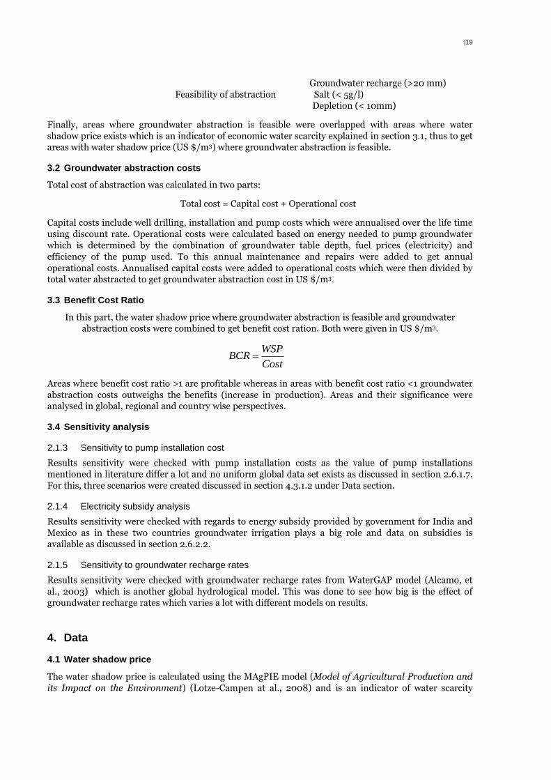
|19

Groundwater recharge (>20 mm)

Feasibility of abstraction Salt (< 5g/l)

Depletion (< 10mm)

Finally, areas where groundwater abstraction is feasible were overlapped with areas where water

shadow price exists which is an indicator of economic water scarcity explained in section 3.1, thus to get

areas with water shadow price (US $/m3) where groundwater abstraction is feasible.

3.2 Groundwater abstraction costs

Total cost of abstraction was calculated in two parts:

Total cost = Capital cost + Operational cost

Capital costs include well drilling, installation and pump costs which were annualised over the life time

using discount rate. Operational costs were calculated based on energy needed to pump groundwater

which is determined by the combination of groundwater table depth, fuel prices (electricity) and

efficiency of the pump used. To this annual maintenance and repairs were added to get annual

operational costs. Annualised capital costs were added to operational costs which were then divided by

total water abstracted to get groundwater abstraction cost in US $/m3.

3.3 Benefit Cost Ratio

In this part, the water shadow price where groundwater abstraction is feasible and groundwater

abstraction costs were combined to get benefit cost ration. Both were given in US $/m3.

WSP

BCRCost

Areas where benefit cost ratio >1 are profitable whereas in areas with benefit cost ratio <1 groundwater

abstraction costs outweighs the benefits (increase in production). Areas and their significance were

analysed in global, regional and country wise perspectives.

3.4 Sensitivity analysis

2.1.3 Sensitivity to pump installation cost

Results sensitivity were checked with pump installation costs as the value of pump installations

mentioned in literature differ a lot and no uniform global data set exists as discussed in section 2.6.1.7.

For this, three scenarios were created discussed in section 4.3.1.2 under Data section.

2.1.4 Electricity subsidy analysis

Results sensitivity were checked with regards to energy subsidy provided by government for India and

Mexico as in these two countries groundwater irrigation plays a big role and data on subsidies is

available as discussed in section 2.6.2.2.

2.1.5 Sensitivity to groundwater recharge rates

Results sensitivity were checked with groundwater recharge rates from WaterGAP model (Alcamo, et

al., 2003) which is another global hydrological model. This was done to see how big is the effect of

groundwater recharge rates which varies a lot with different models on results.

4. Data

4.1 Water shadow price

The water shadow price is calculated using the MAgPIE model (Model of Agricultural Production and

its Impact on the Environment) (Lotze-Campen at al., 2008) and is an indicator of water scarcity

|20

reflecting the amount in US $/m3 a land manager would be willing to pay for relaxing the constraint

(water) by one unit. MAgPIE is a global, spatially explicit model coupled to a grid-based dynamic

vegetation model LPJmL (Bondeau, et al., 2007) to simulate spatially explicit land-use and water-use

patterns with a cost minimisation function developed by the Potsdam Institute for Climate Impact

Research (Lotze-Campe et al., 2008, Biewald et al., 2014). MAgPIE takes socio-economic data for 10

world regions such as population, GDP, food energy demand, average production costs and current self-

sufficiency ratios for food (Lotze‐ Campen et al., 2008) as well as spatially explicit data on potential

crop yields, land and water constraints (from LPJmL) into account. Based on these, the model derives

specific land use patterns, yields and total costs of agricultural production for each grid cell. MAgPIE

simulates 18 cropping and 5 livestock activities with the goal of minimising the global production costs

constrained by availability of resources, namely water and land, and requires that agricultural demands

be met. MAgPIE simulates time steps of 10 years starting in 1995 and uses the optimal land use pattern

from the previous period as a starting point. Each grid cell is assigned to one of the 10 economic world

regions (Figure 6): Sub-Saharan Africa (AFR), Centrally Planned Asia Including China (CPA), Europe

including Turkey (EUR), the newly independent states of the former soviet Union (FSU), Latin America

(LAM), Middle East/North Africa (MEA), North America (NAM), Pacific OECD including Japan,

Australia, New Zealand (PAO); Pacific Asia (PAS) and South Asia Including India (SAS).

Figure 6: Global classification of countries into 10 MAgPIE economic regions

To fulfil the food energy demand in each time step which is an exogenous input based on country and

region specific income, MAgPIE increases production. Production in MAgPIE can be increased through:

expansion of area under cultivation, intensification of agriculture on existing cropland which is achieved

by investment in technological changes and expansion of area equipped for irrigation that leads to

increase in crop yields which this study focuses on. All the processes are also associated with increasing

cost of production due to cost of technology and preparation of land for cropland expansion.

The potential increase in yield with irrigation and amount of water available for irrigation per grid cell is

determined by LPJmL. Yields could also increase with technological changes modelled by MAgPIE.

When all the available water in a grid cell is used for irrigation, the model computes a shadow price for

binding constraints in specific grid cells related to land and water availability. The shadow prices define

the potential cost savings the model would achieve by relaxing the constraint by one unit which in our

study reflects the implicit economic value for one additional cubic meter of water in a particular grid cell

for irrigation (Schmitz, et al., 2013). In case of irrigation, the binding constraint is the available water

thus the shadow price estimates how much an additional unit of water would be worth in the model

context. It is the result of the function minimising the cost of expanding cultivated area, technological

change and water availability.

|21

To analyse the benefit cost ratio of groundwater abstraction for irrigation, two changes were made in

the MAgPIE model. First, the model simulated shadow prices on the entire cropland area, not only on

area where irrigation infrastructure is currently present. To do this, artificial irrigation infrastructure

was given to all the crop land area to make them capable to use available blue water which is the sum of

surface and groundwater. This was needed to analyse the cost benefit of expanding groundwater

irrigation to areas where there is no irrigation present along with areas where irrigation is present but

groundwater abstraction potential is still not fully developed. Second, a groundwater module was

introduced which divided the water availability into surface water and groundwater recharge as input

from the LPJmL (section 3.2.1). Surface water availability from LPJmL is determined in MAgPIE with

the constraint that it is available only during the crop growing period whereas groundwater is made

available all year around. For the places where not all the groundwater recharge is being used,

groundwater availability was replaced with real groundwater abstractions of year 2005 (section 3.2.3.4)

to reflect the price of additional groundwater abstraction and for places where non-renewable

groundwater is being used (abstraction > recharge), groundwater availability was kept equal to

renewable groundwater recharge to reflect the price of non-renewable groundwater (section 3.2.1).

Groundwater availability = Minimum of groundwater recharge and abstraction

These modifications provided the value of water after the total abstraction of surface as well as groundwater in order to establish the benefit-cost ratio for the year 2005.

4.2 Groundwater abstraction feasibility

4.2.1 Groundwater recharge

Global groundwater recharge estimates are taken from Lund-Potsdam-Jena dynamic global vegetation

model with managed lands (LPJmL) (Bondeau, et al., 2007) which simulates biophysical and

biogeochemical processes as well as productivity and yield of the most important crops worldwide.

LPJmL computes the growth and productivity of the world’s major vegetation, nine natural plant

functional types and 12 crop functional types, in direct coupling with associated fluxes of water and

carbon on the vegetation-soil system typically on a global 0.5° grid and at daily time steps (Porkka et

al.,2016). The input data are spatially explicit time series at global 0.5 x 0.5° grid cells of climate, human

land use, soil properties, and river flow directions.

The hydrology scheme of water routing in LPJmL simulates water movement through five fixed depth

soil layers (Figure 7). Gridded soil parameters derived from texture characteristics govern the hydraulic

properties from which top layer infiltration, surface runoff and the subsurface percolation are

calculated. The water reaching the bottom layer is the groundwater recharge which flows into two

groundwater reservoirs with 95% in the top layer representing shallow groundwater and 5% in the

bottom layer which represents deeper stores of the groundwater reservoir with limited hydraulic

connection with surface water. Outflow (natural groundwater discharge) is given by a base flow

recession coefficient as a fraction of the existing groundwater store (Gerten et al., 2013).

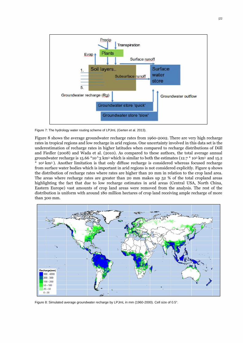
|22

Figure 7: The hydrology water routing scheme of LPJmL (Gerten et al. 2013).

Figure 8 shows the average groundwater recharge rates from 1960-2002. There are very high recharge

rates in tropical regions and low recharge in arid regions. One uncertainty involved in this data set is the

underestimation of recharge rates in higher latitudes when compared to recharge distributions of Döll

and Fiedler (2008) and Wada et al. (2010). As compared to these authors, the total average annual

groundwater recharge is 15.66 *10^3 km3 which is similar to both the estimates (12.7 * 103 km3 and 15.2

* 103 km3 ). Another limitation is that only diffuse recharge is considered whereas focused recharge

from surface water bodies which is important in arid regions is not considered explicitly. Figure 9 shows

the distribution of recharge rates where rates are higher than 20 mm in relation to the crop land area.

The areas where recharge rates are greater than 20 mm makes up 52 % of the total cropland areas

highlighting the fact that due to low recharge estimates in arid areas (Central USA, North China,

Eastern Europe) vast amounts of crop land areas were removed from the analysis. The rest of the

distribution is uniform with around 180 million hectares of crop land receiving ample recharge of more

than 300 mm.

Figure 8: Simulated average groundwater recharge by LPJmL in mm (1960-2000). Cell size of 0.5°.

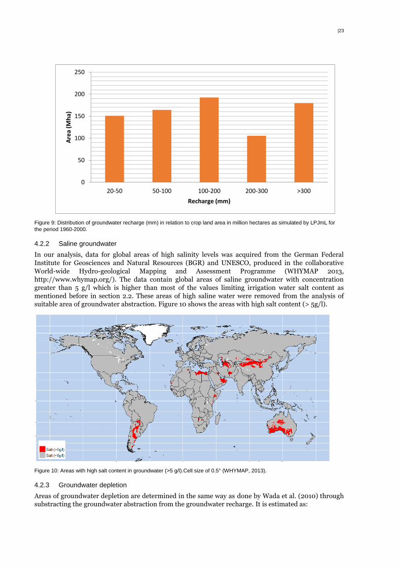
|23

Figure 9: Distribution of groundwater recharge (mm) in relation to crop land area in million hectares as simulated by LPJmL for

the period 1960-2000.

4.2.2 Saline groundwater

In our analysis, data for global areas of high salinity levels was acquired from the German Federal

Institute for Geosciences and Natural Resources (BGR) and UNESCO, produced in the collaborative

World-wide Hydro-geological Mapping and Assessment Programme (WHYMAP 2013,

http://www.whymap.org/). The data contain global areas of saline groundwater with concentration

greater than 5 g/l which is higher than most of the values limiting irrigation water salt content as

mentioned before in section 2.2. These areas of high saline water were removed from the analysis of

suitable area of groundwater abstraction. Figure 10 shows the areas with high salt content (> 5g/l).

Figure 10: Areas with high salt content in groundwater (>5 g/l).Cell size of 0.5° (WHYMAP, 2013).

4.2.3 Groundwater depletion

Areas of groundwater depletion are determined in the same way as done by Wada et al. (2010) through

substracting the groundwater abstraction from the groundwater recharge. It is estimated as:

0

50

100

150

200

250

20-50 50-100 100-200 200-300 >300

Are

a (M

ha)

Recharge (mm)

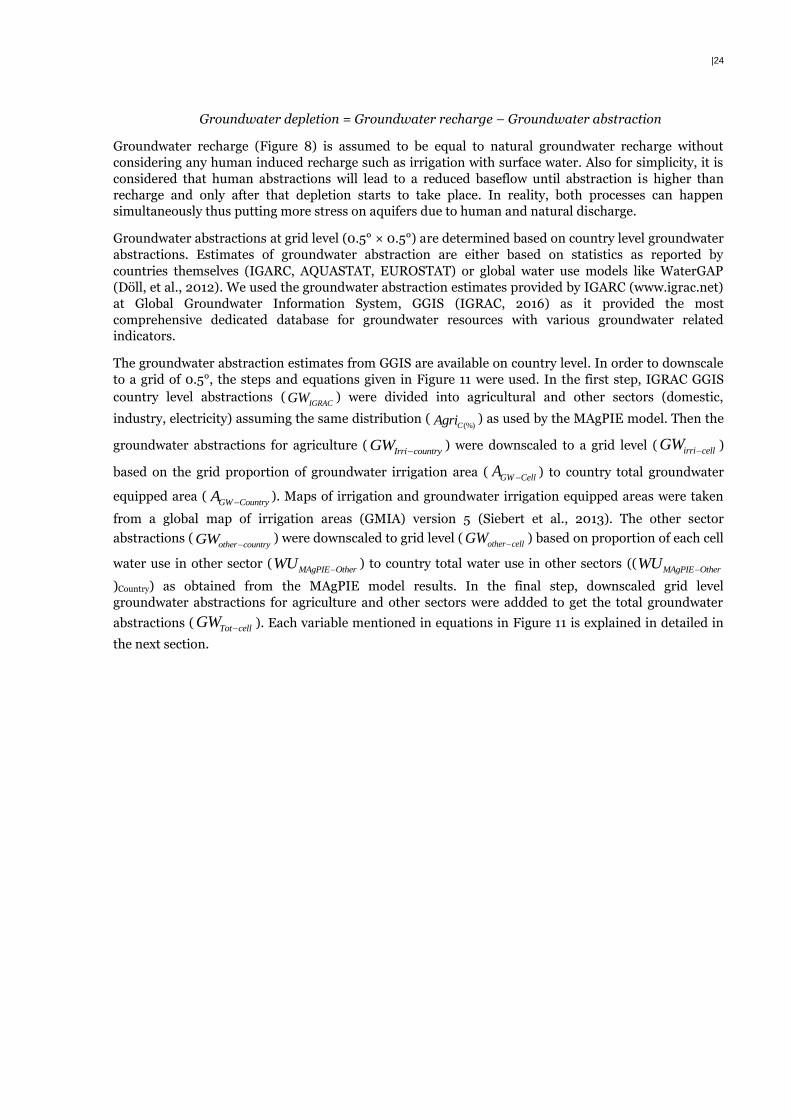
|24

Groundwater depletion = Groundwater recharge – Groundwater abstraction

Groundwater recharge (Figure 8) is assumed to be equal to natural groundwater recharge without

considering any human induced recharge such as irrigation with surface water. Also for simplicity, it is

considered that human abstractions will lead to a reduced baseflow until abstraction is higher than

recharge and only after that depletion starts to take place. In reality, both processes can happen

simultaneously thus putting more stress on aquifers due to human and natural discharge.

Groundwater abstractions at grid level (0.5° × 0.5°) are determined based on country level groundwater

abstractions. Estimates of groundwater abstraction are either based on statistics as reported by

countries themselves (IGARC, AQUASTAT, EUROSTAT) or global water use models like WaterGAP

(Döll, et al., 2012). We used the groundwater abstraction estimates provided by IGARC (www.igrac.net)

at Global Groundwater Information System, GGIS (IGRAC, 2016) as it provided the most

comprehensive dedicated database for groundwater resources with various groundwater related

indicators.

The groundwater abstraction estimates from GGIS are available on country level. In order to downscale

to a grid of 0.5°, the steps and equations given in Figure 11 were used. In the first step, IGRAC GGIS

country level abstractions (IGRACGW ) were divided into agricultural and other sectors (domestic,

industry, electricity) assuming the same distribution ((%)CAgri ) as used by the MAgPIE model. Then the

groundwater abstractions for agriculture (Irri countryGW

) were downscaled to a grid level ( irri cellGW )

based on the grid proportion of groundwater irrigation area ( GW CellA ) to country total groundwater

equipped area (GW CountryA

). Maps of irrigation and groundwater irrigation equipped areas were taken

from a global map of irrigation areas (GMIA) version 5 (Siebert et al., 2013). The other sector

abstractions (other countryGW

) were downscaled to grid level (other cellGW

) based on proportion of each cell

water use in other sector (MAgPIE OtherWU

) to country total water use in other sectors ((MAgPIE OtherWU

)Country) as obtained from the MAgPIE model results. In the final step, downscaled grid level

groundwater abstractions for agriculture and other sectors were addded to get the total groundwater

abstractions ( Tot cellGW ). Each variable mentioned in equations in Figure 11 is explained in detailed in

the next section.

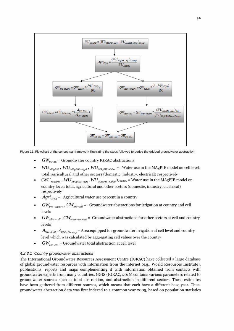
|25

Figure 11: Flowchart of the conceptual framework illustrating the steps followed to derive the gridded groundwater abstraction.

IGRACGW = Groundwater country IGRAC abstractions

MAgPIEWU ,

MAgPIE AgriWU ,

MAgPIE OtherWU = Water use in the MAgPIE model on cell level:

total, agricultural and other sectors (domestic, industry, electrical) respectively

(MAgPIEWU ,

MAgPIE AgriWU ,

MAgPIE OtherWU )Country = Water use in the MAgPIE model on

country level: total, agricultural and other sectors (domestic, industry, electrical)

respectively

(%)CAgri = Agricultural water use percent in a country

Irri countryGW

, irri cellGW = Groundwater abstractions for irrigation at country and cell

levels

other cellGW ,other countryGW

= Groundwater abstractions for other sectors at cell and country

levels

GW CellA ,GW CountryA

= Area equipped for groundwater irrigation at cell level and country

level which was calculated by aggregating cell values over the country

Tot cellGW = Groundwater total abstraction at cell level

4.2.3.1 Country groundwater abstractions

The International Groundwater Resources Assessment Centre (IGRAC) have collected a large database

of global groundwater resources with information from the internet (e.g., World Resources Institute),

publications, reports and maps complementing it with information obtained from contacts with

groundwater experts from many countries. GGIS (IGRAC, 2016) contains various parameters related to

groundwater sources such as total abstraction, and abstraction in different sectors. These estimates

have been gathered from different sources, which means that each have a different base year. Thus,

groundwater abstraction data was first indexed to a common year 2005, based on population statistics

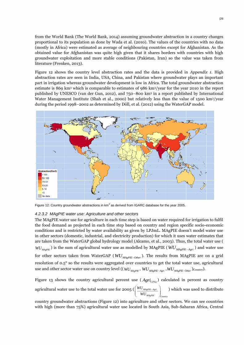
|26

from the World Bank (The World Bank, 2014) assuming groundwater abstraction in a country changes

proportional to its population as done by Wada et al. (2010). The values of the countries with no data

(mostly in Africa) were estimated as average of neighbouring countries except for Afghanistan. As the

obtained value for Afghanistan was quite high given that it shares borders with countries with high

groundwater exploitation and more stable conditions (Pakistan, Iran) so the value was taken from

literature (Frenken, 2013).

Figure 12 shows the country level abstraction rates and the data is provided in Appendix 1. High

abstraction rates are seen in India, USA, China, and Pakistan where groundwater plays an important

part in irrigation whereas groundwater development is low in Africa. The total groundwater abstraction

estimate is 869 km3 which is comparable to estimates of 986 km3/year for the year 2010 in the report

published by UNESCO (van der Gun, 2012), and 750–800 km3 in a report published by International

Water Management Institute (Shah et al., 2000) but relatively less than the value of 1500 km3/year

during the period 1998–2002 as determined by Döll, et al. (2012) using the WaterGAP model.

Figure 12: Country groundwater abstractions in km3 as derived from IGARC database for the year 2005.

4.2.3.2 MAgPIE water use: Agriculture and other sectors

The MAgPIE water use for agriculture in each time step is based on water required for irrigation to fulfil

the food demand as projected in each time step based on country and region specific socio-economic

conditions and is restricted by water availability as given by LPJmL. MAgPIE doesn’t model water use

in other sectors (domestic, industrial, and electricity production) for which it uses water estimates that

are taken from the WaterGAP global hydrology model (Alcamo, et al., 2003). Thus, the total water use (

MAgPIEWU ) is the sum of agricultural water use as modelled by MAgPIE (MAgPIE AgriWU

) and water use

for other sectors taken from WaterGAP (MAgPIE OtherWU

). The results from MAgPIE are on a grid

resolution of 0.5° so the results were aggregated over countries to get the total water use, agricultural

use and other sector water use on country level ((MAgPIEWU ,

MAgPIE AgriWU ,

MAgPIE OtherWU )Country).

Figure 13 shows the country agricultural percent use ((%)CAgri ) calculated in percent as country

agricultural water use to the total water use for 2005 ( MAgPIE Agri

MAgPIE Country

WU

WU

) which was used to distribute

country groundwater abstractions (Figure 12) into agriculture and other sectors. We can see countries

with high (more than 75%) agricultural water use located in South Asia, Sub-Saharan Africa, Central

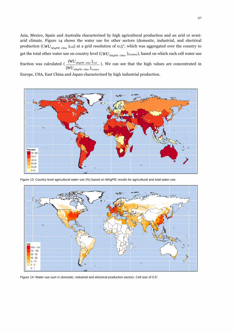
|27

Asia, Mexico, Spain and Australia characterised by high agricultural production and an arid or semi-

arid climate. Figure 14 shows the water use for other sectors (domestic, industrial, and electrical

production ((MAgPIE OtherWU

)Cell) at a grid resolution of 0.5°, which was aggregated over the country to

get the total other water use on country level ((MAgPIE OtherWU

)Country), based on which each cell water use

fraction was calculated (( )

( )

MAgPIE other Cell

MAgPIE Other Country

WU

WU

). We can see that the high values are concentrated in

Europe, USA, East China and Japan characterized by high industrial production.

Figure 13: Country level agricultural water use (%) based on MAgPIE results for agricultural and total water use.

Figure 14: Water use sum in domestic, industrial and electrical production sectors. Cell size of 0.5°.

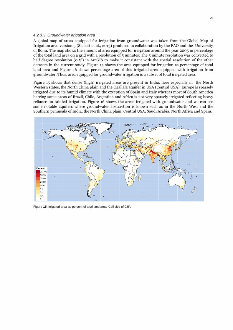
|28

4.2.3.3 Groundwater irrigation area

A global map of areas equipped for irrigation from groundwater was taken from the Global Map of

Irrigation area version 5 (Siebert et al., 2013) produced in collaboration by the FAO and the University

of Bonn. The map shows the amount of area equipped for irrigation around the year 2005 in percentage

of the total land area on a grid with a resolution of 5 minutes. The 5 minute resolution was converted to

half degree resolution (0.5°) in ArcGIS to make it consistent with the spatial resolution of the other

datasets in the current study. Figure 15 shows the area equipped for irrigation as percentage of total

land area and Figure 16 shows percentage area of this irrigated area equipped with irrigation from

groundwater. Thus, area equipped for groundwater irrigation is a subset of total irrigated area.

Figure 15 shows that dense (high) irrigated areas are present in India, here especially in the North

Western states, the North China plain and the Ogallala aquifer in USA (Central USA). Europe is sparsely

irrigated due to its humid climate with the exception of Spain and Italy whereas most of South America

barring some areas of Brazil, Chile, Argentina and Africa is not very sparsely irrigated reflecting heavy

reliance on rainfed irrigation. Figure 16 shows the areas irrigated with groundwater and we can see

some notable aquifers where groundwater abstraction is known such as in the North West and the

Southern peninsula of India, the North China plain, Central USA, Saudi Arabia, North Africa and Spain.

Figure 15: Irrigated area as percent of total land area. Cell size of 0.5°.

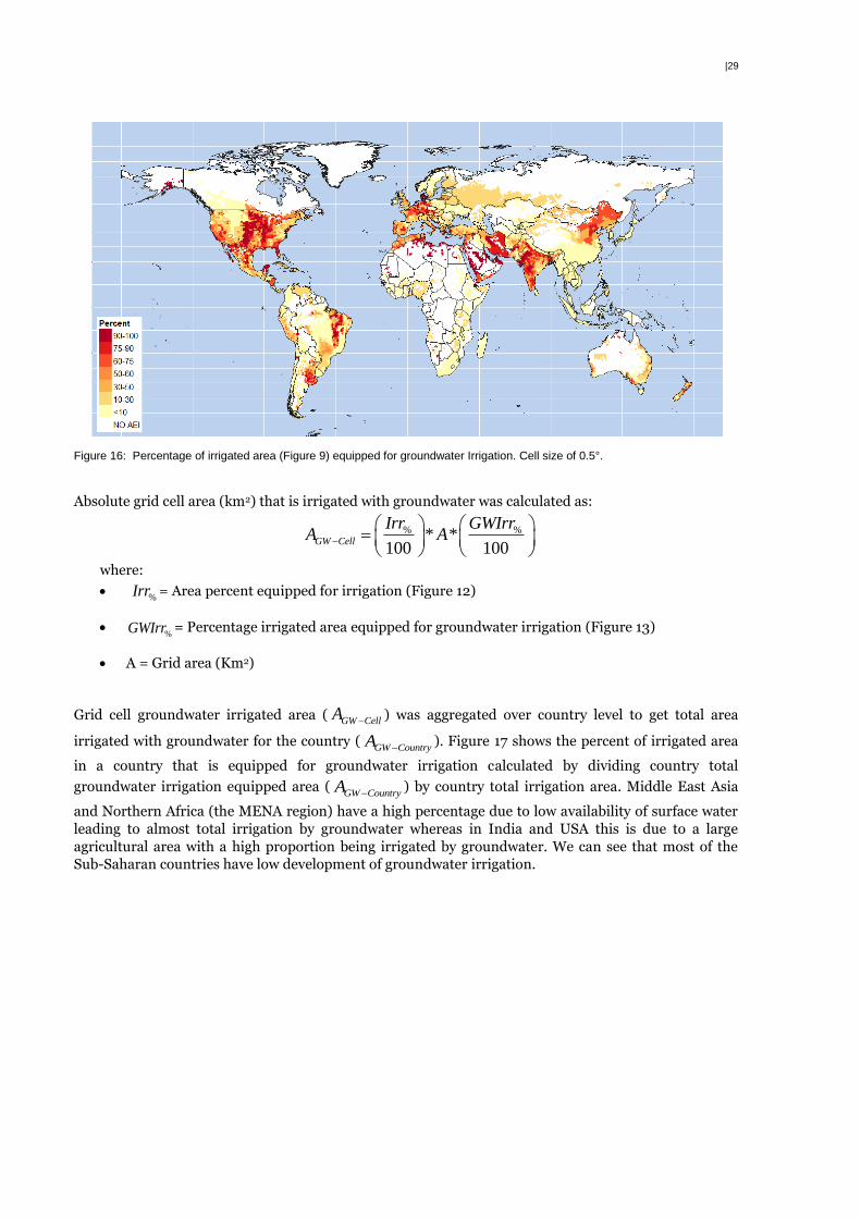
|29

Figure 16: Percentage of irrigated area (Figure 9) equipped for groundwater Irrigation. Cell size of 0.5°.

Absolute grid cell area (km2) that is irrigated with groundwater was calculated as:

% %* *100 100

GW Cell

Irr GWIrrA A

where:

%Irr = Area percent equipped for irrigation (Figure 12)

%GWIrr = Percentage irrigated area equipped for groundwater irrigation (Figure 13)

A = Grid area (Km2)

Grid cell groundwater irrigated area ( GW CellA ) was aggregated over country level to get total area

irrigated with groundwater for the country (GW CountryA

). Figure 17 shows the percent of irrigated area

in a country that is equipped for groundwater irrigation calculated by dividing country total

groundwater irrigation equipped area (GW CountryA

) by country total irrigation area. Middle East Asia

and Northern Africa (the MENA region) have a high percentage due to low availability of surface water

leading to almost total irrigation by groundwater whereas in India and USA this is due to a large

agricultural area with a high proportion being irrigated by groundwater. We can see that most of the

Sub-Saharan countries have low development of groundwater irrigation.

|30

Figure 17: Percentage groundwater equipped irrigated area in relation to total irrigated area per country.

4.2.3.4 Gridded groundwater abstractions

Groundwater abstracted at grid level ( Tot cellGW ) calculated is shown in Figure 18. We can see that high

abstraction coincides with densely groundwater irrigated areas such as in the North India Gangetic

plains, Central USA and the North China plain. This has resulted in groundwater depletion in these

areas, whereas we can see that groundwater use is not much developed in Sub-Saharan Africa and

South America.

Figure 18: Total groundwater abstractions in mm calculated as sum of groundwater abstractions in agricultural and other sectors

(domestic, industry, electricity production). Cell size of 0.5°.

4.2.3.5 Gridded groundwater depletion

Areas of groundwater depletion are shown in Figure 19, and due to uncertainties involved in both

abstraction and recharge estimates, only areas with more than 10 mm of depletion are considered as

areas of groundwater depletion. Figure 16 shows the depletion in notable groundwater aquifers as

reported in the literature such as North West India (Rodell et al., 2009) and North East Pakistan, The

|31

North China plain aquifer (Changming et al., 2001), Ogallala aquifer in the High plains of USA

(Scanlona, et al., 2012), the Cental Valley of Califronia (Famiglietti, et al., 2011), and Iran (Joodaki et al.,

2014). Non renewable groundwater mining occurs in Saudi Arabia and Northern Africa (Foster &

Loucks, 2006), Mexico (Scott, 2011), Beauce Aquifer in Central France (Barraqué et al., 2010), and

South East Spain (Llamas et al., 2015). These areas were removed from the analysis considering that

they are already over-exploited.

Figure 19: Groundwater depletion in mm calculated as difference between groundwater recharge and abstractions. Cell size of

0.5°.

4.3 Groundwater abstraction costs

In this study, total cost of abstraction was calculated in two parts as done by others as mentioned in

section 2.6:

Total cost = Capital cost + Operational cost

4.3.1 Capital costs

Capital costs included pump costs, well drilling and installation. Capital costs were annualised over the

life time using a discount rate and added to operational costs, which were then divided by the total

water abstracted to get the cost per cubic metre.

4.3.1.1 Pump selection and price for analysis

For our study, we selected pumps on two criteria: Energy source (section 2.6.1.1) and operation

principle (section 2.6.1.2). Then, pump performance curves (section 2.6.1.3) were used to get pumps

based on depth and flow requirement.

Based on energy source, we have focused on the costs of pumping using electric pumps for the following

reasons discussed in more detail in section 2.6.1.1:

Low operating costs over diesel pumps, low maintenance and high efficiency

High initial capital cost and low penetration associated with solar powered pumps

The range of depths with diesel and solar powered pumps are mostly limited to shallow depths

Thus, we assume that electric connection and reliable power is available at the farm level which is still

not the case in developing countries where electrification rates are low and power cuts frequent.

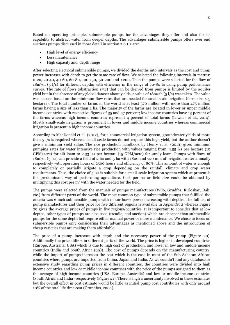
|32

Based on operating principle, submersible pumps for the advantages they offer and also for its

capability to abstract water from deeper depths. The advantages submersible pumps offers over end

suctions pumps discussed in more detail in section 2.6.1.2 are:

High level of energy efficiency

Less maintenance

High capacity and depth range

After selecting electrical submersible pumps, we divided the depths into intervals as the cost and pump

power increases with depth to get the same rate of flow. We selected the following intervals in metres:

0-20, 20-40, 40-60, 60-80, 100-150,150-200 and >200. Then the pumps were selected for the flow of

18m3/h (5 l/s) for different depths with efficiency in the range of 70-80 % using pump performance

curves. The rate of flows (abstraction rate) that can be derived from pumps is limited by the aquifer

yield but in the absence of any global dataset about yields, a value of 18m3/h (5 l/s) was taken. The value

was chosen based on the minimum flow rates that are needed for small scale irrigation (farm size < 5

hectares). The total number of farms in the world is at least 570 million with more than 475 million

farms having a size of less than 2 ha. The majority of the farms are located in lower or upper middle

income countries with respective figures of 35 and 47 percent; low income countries have 13 percent of

the farms whereas high income countries represent 4 percent of total farms (Lowder et al., 2014).

Mostly small-scale irrigation is prominent in lower and middle income countries whereas commercial

irrigation is present in high income countries.

According to MacDonald et al. (2012), for a commercial irrigation system, groundwater yields of more

than 5 l/s is required whereas small-scale farms do not require this high yield, but the author doesn’t

give a minimum yield value. The rice production handbook by Henry et al. (2013) gives minimum

pumping rates for water intensive rice production with values ranging from 1.55 l/s per hectare (10

GPM/acre) for silt loam to 2.33 l/s per hectare (15 GPM/acre) for sandy loam. Pumps with flows of

18m3/h (5 l/s) can provide a field of 2 ha and 5 ha with 1800 and 720 mm of irrigation water annually

respectively with operating hours of 2500 hours and efficiency of 80%. This amount of water is enough

to completely or partially irrigate a crop depending on the rainfall, climate and crop water

requirements. Thus, the choice of 5 l/s is suitable for a small-scale irrigation system which at present is

the predominant way of performing agriculture. Cost per ha or field size could be obtained by

multiplying this cost per m3 with the water needed for the field.

The pumps were selected from the manuals of pumps manufactures (Wilo, Grudfos, Kirloskar, Dab,

etc.) from different parts of the world. The most common type of submersible pumps that fulfilled the

criteria was 6 inch submersible pumps with motor horse power increasing with depths. The full list of

pump manufactures and their price for five different regions is available in Appendix 2 whereas Figure

20 gives the average prices of pumps in five regions/countries. It is important to consider that at low

depths, other types of pumps are also used (treadle, end suction) which are cheaper than submersible

pumps for the same depth but require either manual power or more maintenance. We chose to focus on

submersible pumps only considering their advantages as mentioned above and the introduction of

cheap varieties that are making them affordable.

The price of a pump increases with depth and the necessary power of the pump (Figure 20).

Additionally the price differs in different parts of the world. The price is higher in developed countries

(Europe, Australia, USA) which is due to high cost of production, and lower in low and middle income

countries (India and South Africa (SA)). The cost of pumps depends on the manufacturing country,

while the import of pumps increases the cost which is the case in most of the Sub-Saharan African

countries where pumps are imported from China, Japan and India. As we couldn’t find any database or

extensive study regarding pump prices in different countries, the countries were divided into high

income countries and low or middle income countries with the price of the pumps assigned to them as

the average of high income countries (USA, Europe, Australia) and low or middle income countries

(South Africa and India) respectively (Figure 21). There is high a uncertainty involved in these estimates

but the overall effect in cost estimate would be little as initial pump cost contributes with only around

10% of the total life time cost (Grundfos, 2004).

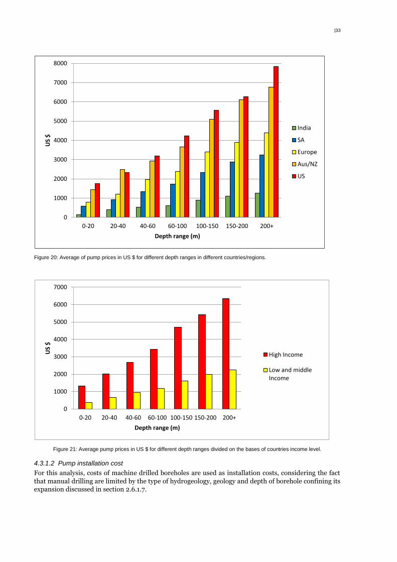
|33

Figure 20: Average of pump prices in US $ for different depth ranges in different countries/regions.

Figure 21: Average pump prices in US $ for different depth ranges divided on the bases of countries income level.

4.3.1.2 Pump installation cost

For this analysis, costs of machine drilled boreholes are used as installation costs, considering the fact

that manual drilling are limited by the type of hydrogeology, geology and depth of borehole confining its

expansion discussed in section 2.6.1.7.

0

1000

2000

3000

4000

5000

6000

7000

8000

0-20 20-40 40-60 60-100 100-150 150-200 200+

US

$

Depth range (m)

India

SA

Europe

Aus/NZ

US

0

1000

2000

3000

4000

5000

6000

7000

0-20 20-40 40-60 60-100 100-150 150-200 200+

US

$

Depth range (m)

High Income

Low and middle Income

|34

Cost of borehole installation varies from 18 $/m to 500 $/m with an average of 120 $/m as given in

Table 3 from different sources. As the cost reported is for machine drilling only, there would be much

more variation if the cost of manual drilling was included which are cheaper than machine drilling. Due

to the high uncertainty in the costs, three scenarios were analysed with cost per metre of borehole

development at US $ 50, 100 and 200 per metre. The scenario with 100 US $/m is referred to as the

default scenario further on.

4.3.1.3 Annuity of capital cost

To calculate the annuity of initial capital investment in US $/year, the equivalent annual cost method is

used as mentioned in detailed in section 2.6.1.8. The equivalent annual cost (EAC) is calculated as:

*

1 (1 ) T

P REAC

R

where:

P = Asset price or initial capital cost

R = Discount rate

T = Life time period

Considering the various discount values reported as given in section 2.6.1.8, a discount rate of 3.5 % was

used, which is recommend by the UK green book (HM Treasury, 2003) for a time horizon of up to 30

years.

The life span of pump systems used in studies range from 10 to 25 years with more studies gravitating

towards a life span of 10 years as this is considered to be the economic life span of pumps according to

the users as given in section 2.6.1.8. A value of 10 years was used in the study as this is also close to the

value of 11 years reported for multistage submersible pumps in the study conducted for the European

Commission (Falkner, 2008).

4.3.2 Operational costs

The operational costs of running a pump are the costs incurred on electricity prices needed to pump

which depends on the pump, pumping depth and efficiency, and to this maintenance and repair costs

are added.

The cost of electricity needed for pumping is determined by the total energy consumed which depends

on the power used and the number of operating hours of the pump, which gives the total energy

consumed in kilowatt hours (kWh). The power used for the abstraction of water is determined by flow

rate (pumping rate), depth to groundwater and efficiency of pump and motor given by the formula

(Hydaulic Institute, Europump, US Depatment of Energy, 2001):

Operational cost = Electricity cost + Maintenance & repair

Electricity cost = E * P

* * .g.*T

366* *p m

Q H sE

where:

E = energy (kWh)

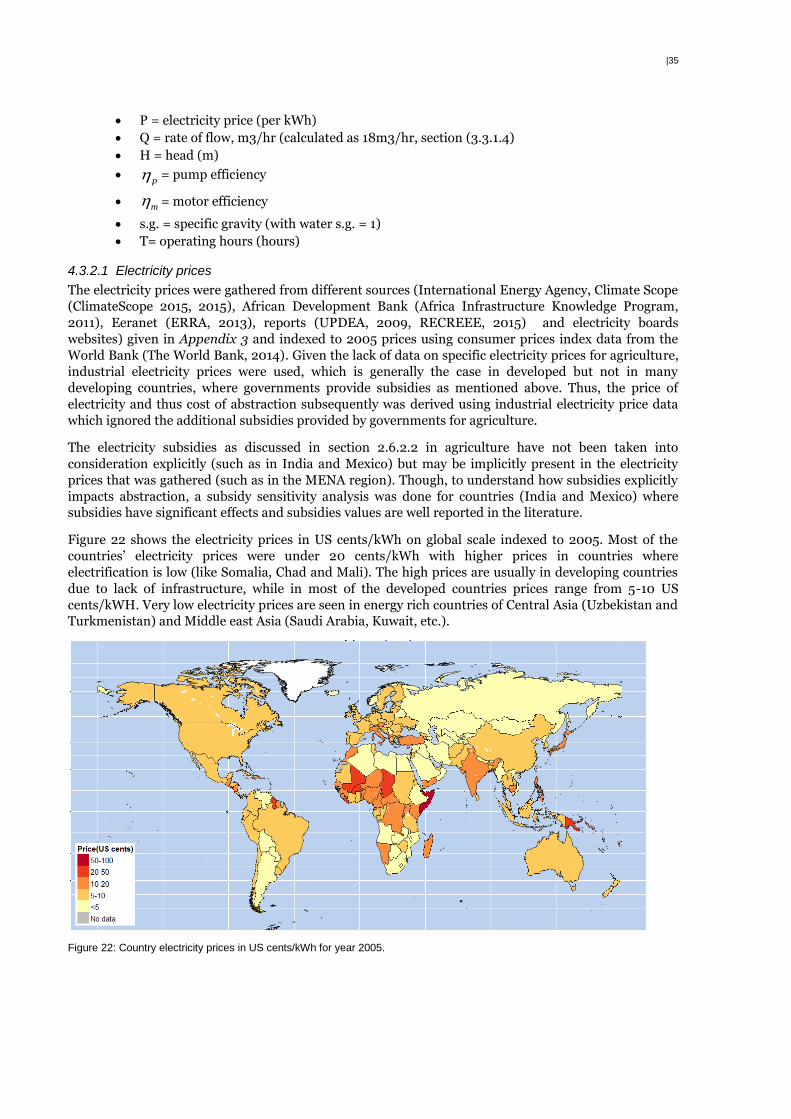
|35

P = electricity price (per kWh)

Q = rate of flow, m3/hr (calculated as 18m3/hr, section (3.3.1.4)

H = head (m)

p = pump efficiency

m = motor efficiency

s.g. = specific gravity (with water s.g. = 1)

T= operating hours (hours)

4.3.2.1 Electricity prices

The electricity prices were gathered from different sources (International Energy Agency, Climate Scope

(ClimateScope 2015, 2015), African Development Bank (Africa Infrastructure Knowledge Program,

2011), Eeranet (ERRA, 2013), reports (UPDEA, 2009, RECREEE, 2015) and electricity boards

websites) given in Appendix 3 and indexed to 2005 prices using consumer prices index data from the

World Bank (The World Bank, 2014). Given the lack of data on specific electricity prices for agriculture,

industrial electricity prices were used, which is generally the case in developed but not in many

developing countries, where governments provide subsidies as mentioned above. Thus, the price of

electricity and thus cost of abstraction subsequently was derived using industrial electricity price data

which ignored the additional subsidies provided by governments for agriculture.

The electricity subsidies as discussed in section 2.6.2.2 in agriculture have not been taken into

consideration explicitly (such as in India and Mexico) but may be implicitly present in the electricity

prices that was gathered (such as in the MENA region). Though, to understand how subsidies explicitly

impacts abstraction, a subsidy sensitivity analysis was done for countries (India and Mexico) where

subsidies have significant effects and subsidies values are well reported in the literature.

Figure 22 shows the electricity prices in US cents/kWh on global scale indexed to 2005. Most of the

countries’ electricity prices were under 20 cents/kWh with higher prices in countries where

electrification is low (like Somalia, Chad and Mali). The high prices are usually in developing countries

due to lack of infrastructure, while in most of the developed countries prices range from 5-10 US

cents/kWH. Very low electricity prices are seen in energy rich countries of Central Asia (Uzbekistan and

Turkmenistan) and Middle east Asia (Saudi Arabia, Kuwait, etc.).

Figure 22: Country electricity prices in US cents/kWh for year 2005.

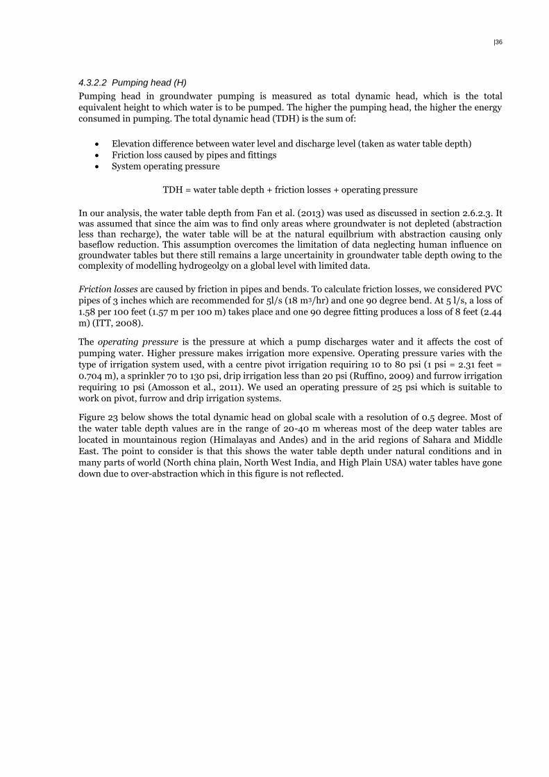
|36

4.3.2.2 Pumping head (H)

Pumping head in groundwater pumping is measured as total dynamic head, which is the total

equivalent height to which water is to be pumped. The higher the pumping head, the higher the energy

consumed in pumping. The total dynamic head (TDH) is the sum of:

Elevation difference between water level and discharge level (taken as water table depth)

Friction loss caused by pipes and fittings

System operating pressure

TDH = water table depth + friction losses + operating pressure

In our analysis, the water table depth from Fan et al. (2013) was used as discussed in section 2.6.2.3. It was assumed that since the aim was to find only areas where groundwater is not depleted (abstraction less than recharge), the water table will be at the natural equilbrium with abstraction causing only baseflow reduction. This assumption overcomes the limitation of data neglecting human influence on groundwater tables but there still remains a large uncertainity in groundwater table depth owing to the complexity of modelling hydrogeolgy on a global level with limited data.

Friction losses are caused by friction in pipes and bends. To calculate friction losses, we considered PVC

pipes of 3 inches which are recommended for 5l/s (18 m3/hr) and one 90 degree bend. At 5 l/s, a loss of

1.58 per 100 feet (1.57 m per 100 m) takes place and one 90 degree fitting produces a loss of 8 feet (2.44

m) (ITT, 2008).

The operating pressure is the pressure at which a pump discharges water and it affects the cost of

pumping water. Higher pressure makes irrigation more expensive. Operating pressure varies with the

type of irrigation system used, with a centre pivot irrigation requiring 10 to 80 psi (1 psi = 2.31 feet =

0.704 m), a sprinkler 70 to 130 psi, drip irrigation less than 20 psi (Ruffino, 2009) and furrow irrigation

requiring 10 psi (Amosson et al., 2011). We used an operating pressure of 25 psi which is suitable to

work on pivot, furrow and drip irrigation systems.

Figure 23 below shows the total dynamic head on global scale with a resolution of 0.5 degree. Most of

the water table depth values are in the range of 20-40 m whereas most of the deep water tables are

located in mountainous region (Himalayas and Andes) and in the arid regions of Sahara and Middle

East. The point to consider is that this shows the water table depth under natural conditions and in

many parts of world (North china plain, North West India, and High Plain USA) water tables have gone

down due to over-abstraction which in this figure is not reflected.

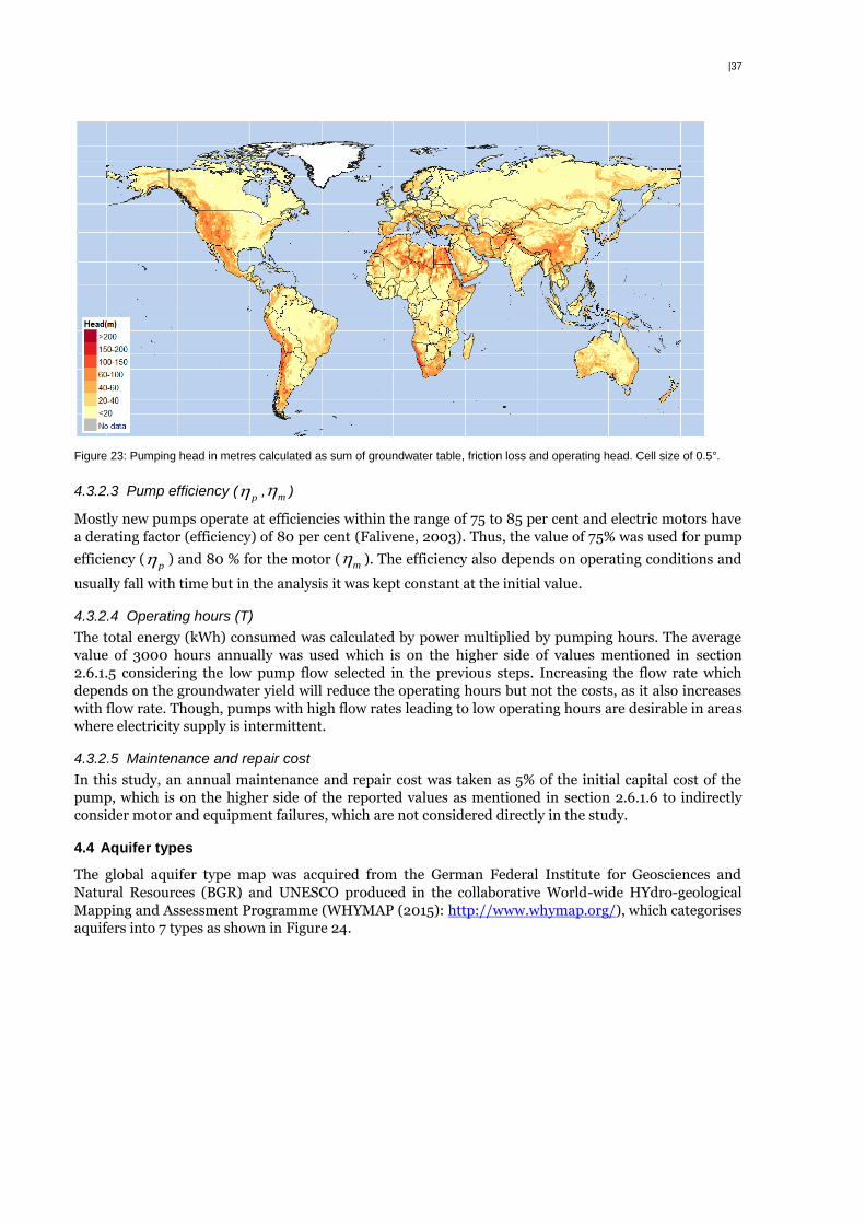
|37

Figure 23: Pumping head in metres calculated as sum of groundwater table, friction loss and operating head. Cell size of 0.5°.

4.3.2.3 Pump efficiency (p , m )

Mostly new pumps operate at efficiencies within the range of 75 to 85 per cent and electric motors have

a derating factor (efficiency) of 80 per cent (Falivene, 2003). Thus, the value of 75% was used for pump

efficiency (p ) and 80 % for the motor ( m ). The efficiency also depends on operating conditions and

usually fall with time but in the analysis it was kept constant at the initial value.

4.3.2.4 Operating hours (T)

The total energy (kWh) consumed was calculated by power multiplied by pumping hours. The average

value of 3000 hours annually was used which is on the higher side of values mentioned in section

2.6.1.5 considering the low pump flow selected in the previous steps. Increasing the flow rate which

depends on the groundwater yield will reduce the operating hours but not the costs, as it also increases

with flow rate. Though, pumps with high flow rates leading to low operating hours are desirable in areas

where electricity supply is intermittent.

4.3.2.5 Maintenance and repair cost

In this study, an annual maintenance and repair cost was taken as 5% of the initial capital cost of the

pump, which is on the higher side of the reported values as mentioned in section 2.6.1.6 to indirectly

consider motor and equipment failures, which are not considered directly in the study.

4.4 Aquifer types

The global aquifer type map was acquired from the German Federal Institute for Geosciences and

Natural Resources (BGR) and UNESCO produced in the collaborative World-wide HYdro-geological

Mapping and Assessment Programme (WHYMAP (2015): http://www.whymap.org/), which categorises

aquifers into 7 types as shown in Figure 24.

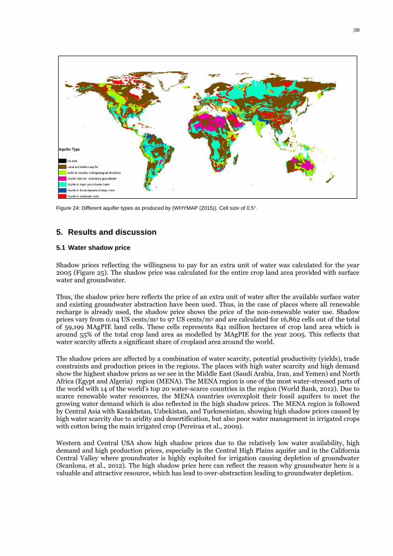
|38

Figure 24: Different aquifer types as produced by (WHYMAP (2015)). Cell size of 0.5°.

5. Results and discussion

5.1 Water shadow price

Shadow prices reflecting the willingness to pay for an extra unit of water was calculated for the year 2005 (Figure 25). The shadow price was calculated for the entire crop land area provided with surface water and groundwater.

Thus, the shadow price here reflects the price of an extra unit of water after the available surface water and existing groundwater abstraction have been used. Thus, in the case of places where all renewable recharge is already used, the shadow price shows the price of the non-renewable water use. Shadow prices vary from 0.04 US cents/m3 to 97 US cents/m3 and are calculated for 16,862 cells out of the total of 59,199 MAgPIE land cells. These cells represents 841 million hectares of crop land area which is around 55% of the total crop land area as modelled by MAgPIE for the year 2005. This reflects that water scarcity affects a significant share of cropland area around the world.

The shadow prices are affected by a combination of water scarcity, potential productivity (yields), trade constraints and production prices in the regions. The places with high water scarcity and high demand show the highest shadow prices as we see in the Middle East (Saudi Arabia, Iran, and Yemen) and North Africa (Egypt and Algeria) region (MENA). The MENA region is one of the most water-stressed parts of the world with 14 of the world’s top 20 water-scarce countries in the region (World Bank, 2012). Due to scarce renewable water resources, the MENA countries overexploit their fossil aquifers to meet the growing water demand which is also reflected in the high shadow prices. The MENA region is followed by Central Asia with Kazakhstan, Uzbekistan, and Turkmenistan, showing high shadow prices caused by high water scarcity due to aridity and desertification, but also poor water management in irrigated crops with cotton being the main irrigated crop (Pereiraa et al., 2009).

Western and Central USA show high shadow prices due to the relatively low water availability, high demand and high production prices, especially in the Central High Plains aquifer and in the California Central Valley where groundwater is highly exploited for irrigation causing depletion of groundwater (Scanlona, et al., 2012). The high shadow price here can reflect the reason why groundwater here is a valuable and attractive resource, which has lead to over-abstraction leading to groundwater depletion.

|39

The high shadow prices in Europe and Australia are due to the high yields that could be achieved by an extra unit of water where water is scarce in these regions. In Southern Europe countries such as Spain and Italy, irrigated agriculture is significant as they are subjected to a semi-arid climate facing strong seasonal variability of precipitation, thus leading to groundwater abstraction. Agricultural use accounts for between 80 and 90% of the water abstraction in basins of the south and in the basins of rivers flowing to the Mediterranean Sea. The semi-arid climate along with valuable groundwater resources reflected in high shadow prices have resulted in a substantial share of the groundwater resources being at risk of being overexploited, such as in Southern Spain (Fuentes, 2011). In comparison, shadow prices are lower in Eastern Europe including Russia. Australia also has an arid and semi-arid climate with limited surface water sources. Water used for agricultural irrigation is the largest single user group, comprising on average approximately 60% of the annual groundwater use (Deloitte Access Economics, 2013), reflected in high shadow prices in most of its cropland area by the South-East and East coast.

In general shadow prices are lower in the developing and least developed countries of Africa, Asia and Latin America in comparison to the developed countries of North America and Europe. One important factor determining shadow prices could be the technological changes, which are still less advanced than in the developed countries and therefore results in lower yield levels. Water shadow prices are lower in India but still high groundwater exploitation exists in these areas. This could be the result of subsidies provided by the government for energy which are not included in the model, as well as unreliable surface water supply. No or very low shadow prices exists in equatorial regions of South America, Central Africa and South East Asia where water is abundant due to high precipitation. In Sub-Saharan Africa, high shadow prices are seen in the southern (South Africa and Namibia) and eastern parts (e.g. Ethiopia and Tanzania) where water is scarce, whereas in central Africa where water precipitation and groundwater recharge is significant no shadow prices exist.

Figure 25: Water shadow prices (WSP) in US cents/m3.

Cell size of 0.5°.

5.2 Groundwater abstraction feasibility

Figure 26 shows the area where groundwater abstraction is possible based on the criteria given as:

Recharge greater than 20 mm

Salt content less than 5 g/l

No groundwater depletion

The total area where groundwater abstraction is feasible is 727 million hectares which is around 47.4 %

of the total crop land area as modelled by MAgPIE for year 2005. This highlights the fact that more than

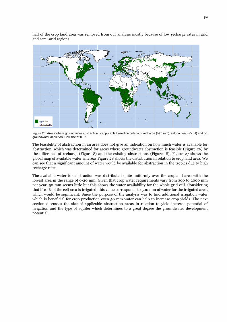
|40

half of the crop land area was removed from our analysis mostly because of low recharge rates in arid

and semi-arid regions.

Figure 26: Areas where groundwater abstraction is applicable based on criteria of recharge (>20 mm), salt content (<5 g/l) and no

groundwater depletion. Cell size of 0.5°.

The feasibility of abstraction in an area does not give an indication on how much water is available for

abstraction, which was determined for areas where groundwater abstraction is feasible (Figure 26) by

the difference of recharge (Figure 8) and the existing abstractions (Figure 18). Figure 27 shows the

global map of available water whereas Figure 28 shows the distribution in relation to crop land area. We

can see that a significant amount of water would be available for abstraction in the tropics due to high

recharge rates.

The available water for abstraction was distributed quite uniformly over the cropland area with the

lowest area in the range of 0-20 mm. Given that crop water requirements vary from 300 to 2000 mm

per year, 50 mm seems little but this shows the water availability for the whole grid cell. Considering

that if 10 % of the cell area is irrigated, this value corresponds to 500 mm of water for the irrigated area,

which would be significant. Since the purpose of the analysis was to find additional irrigation water

which is beneficial for crop production even 50 mm water can help to increase crop yields. The next

section discusses the size of applicable abstraction areas in relation to yield increase potential of

irrigation and the type of aquifer which determines to a great degree the groundwater development

potential.

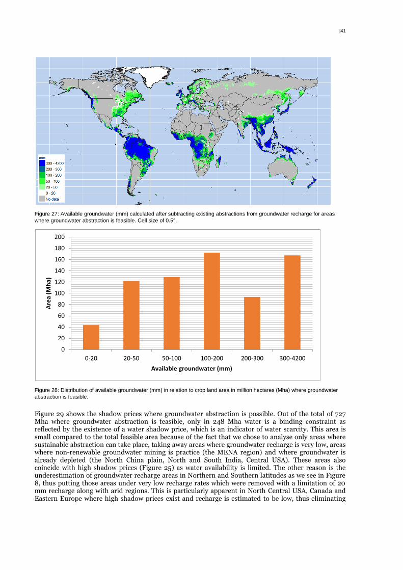
|41

Figure 27: Available groundwater (mm) calculated after subtracting existing abstractions from groundwater recharge for areas

where groundwater abstraction is feasible. Cell size of 0.5°.

Figure 28: Distribution of available groundwater (mm) in relation to crop land area in million hectares (Mha) where groundwater

abstraction is feasible.

Figure 29 shows the shadow prices where groundwater abstraction is possible. Out of the total of 727 Mha where groundwater abstraction is feasible, only in 248 Mha water is a binding constraint as reflected by the existence of a water shadow price, which is an indicator of water scarcity. This area is small compared to the total feasible area because of the fact that we chose to analyse only areas where sustainable abstraction can take place, taking away areas where groundwater recharge is very low, areas where non-renewable groundwater mining is practice (the MENA region) and where groundwater is already depleted (the North China plain, North and South India, Central USA). These areas also coincide with high shadow prices (Figure 25) as water availability is limited. The other reason is the underestimation of groundwater recharge areas in Northern and Southern latitudes as we see in Figure 8, thus putting those areas under very low recharge rates which were removed with a limitation of 20 mm recharge along with arid regions. This is particularly apparent in North Central USA, Canada and Eastern Europe where high shadow prices exist and recharge is estimated to be low, thus eliminating

0

20

40

60

80

100

120

140

160

180

200

0-20 20-50 50-100 100-200 200-300 300-4200

Are

a (M

ha)

Available groundwater (mm)

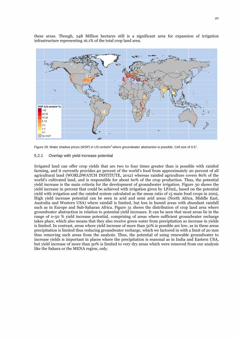
|42

these areas. Though, 248 Million hectares still is a significant area for expansion of irrigation infrastructure representing 16.1% of the total crop land area.

Figure 29: Water shadow prices (WSP) in US cents/m3 where groundwater abstraction is possible. Cell size of 0.5°.

5.2.1 Overlap with yield increase potential

Irrigated land can offer crop yields that are two to four times greater than is possible with rainfed farming, and it currently provides 40 percent of the world’s food from approximately 20 percent of all agricultural land (WORLDWATCH INSTITUTE, 2012) whereas rainfed agriculture covers 80% of the world’s cultivated land, and is responsible for about 60% of the crop production. Thus, the potential yield increase is the main criteria for the development of groundwater irrigation. Figure 30 shows the yield increase in percent that could be achieved with irrigation given by LPJmL, based on the potential yield with irrigation and the rainfed system calculated as the mean ratio of 15 main food crops in 2005. High yield increase potential can be seen in arid and semi arid areas (North Africa, Middle East, Australia and Western USA) where rainfall is limited, but less in humid areas with abundant rainfall such as in Europe and Sub-Saharan Africa. Figure 31 shows the distribution of crop land area where groundwater abstraction in relation to potential yield increases. It can be seen that most areas lie in the range of 0-50 % yield increase potential, comprising of areas where sufficient groundwater recharge takes place, which also means that they also receive green water from precipitation so increase in yields is limited. In contrast, areas where yield increase of more than 50% is possible are low, as in these areas precipitation is limited thus reducing groundwater recharge, which we factored in with a limit of 20 mm thus removing such areas from the analysis. Thus, the potential of using renewable groundwater to increase yields is important in places where the precipitation is seasonal as in India and Eastern USA, but yield increase of more than 50% is limited to very dry areas which were removed from our analysis like the Sahara or the MENA region, only.

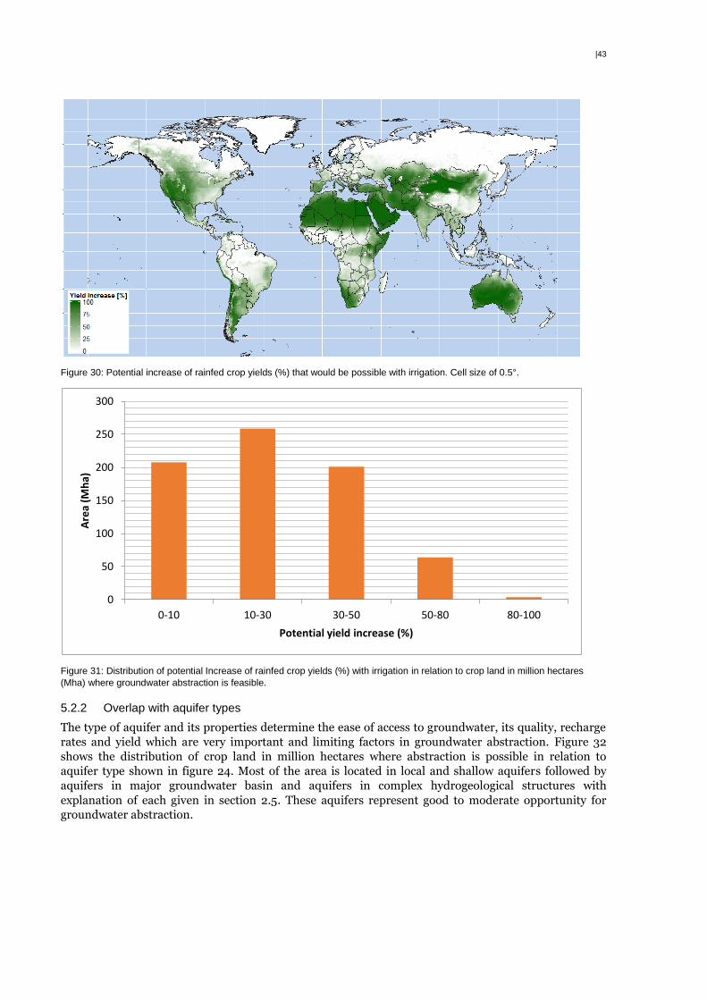
|43

Figure 30: Potential increase of rainfed crop yields (%) that would be possible with irrigation. Cell size of 0.5°.

Figure 31: Distribution of potential Increase of rainfed crop yields (%) with irrigation in relation to crop land in million hectares

(Mha) where groundwater abstraction is feasible.

5.2.2 Overlap with aquifer types

The type of aquifer and its properties determine the ease of access to groundwater, its quality, recharge

rates and yield which are very important and limiting factors in groundwater abstraction. Figure 32

shows the distribution of crop land in million hectares where abstraction is possible in relation to

aquifer type shown in figure 24. Most of the area is located in local and shallow aquifers followed by

aquifers in major groundwater basin and aquifers in complex hydrogeological structures with

explanation of each given in section 2.5. These aquifers represent good to moderate opportunity for

groundwater abstraction.

0

50

100

150

200

250

300

0-10 10-30 30-50 50-80 80-100

Are

a (M

ha)

Potential yield increase (%)

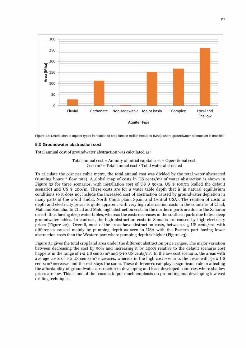
|44

Figure 32: Distribution of aquifer types in relation to crop land in million hectares (Mha) where groundwater abstraction is feasible.

5.3 Groundwater abstraction cost

Total annual cost of groundwater abstraction was calculated as:

Total annual cost = Annuity of initial capital cost + Operational cost

Cost/m3 = Total annual cost / Total water abstracted

To calculate the cost per cubic metre, the total annual cost was divided by the total water abstracted

(running hours * flow rate). A global map of costs in US cents/m3 of water abstraction is shown in

Figure 33 for three scenarios, with installation cost of US $ 50/m, US $ 100/m (called the default

scenario) and US $ 200/m. These costs are for a water table depth that is in natural equilibrium

conditions so it does not include the increased cost of abstraction caused by groundwater depletion in

many parts of the world (India, North China plain, Spain and Central USA). The relation of costs to

depth and electricity prices is quite apparent with very high abstraction costs in the countries of Chad,

Mali and Somalia. In Chad and Mali, high abstraction costs in the northern parts are due to the Saharan

desert, thus having deep water tables, whereas the costs decreases in the southern parts due to less deep

groundwater tables. In contrast, the high abstraction costs in Somalia are caused by high electricity

prices (Figure 22). Overall, most of the areas have abstraction costs, between 2-5 US cents/m3, with

differences caused mainly by pumping depth as seen in USA with the Eastern part having lower

abstraction costs than the Western part where pumping depth is higher (Figure 23).

Figure 34 gives the total crop land area under the different abstraction price ranges. The major variation

between decreasing the cost by 50% and increasing it by 200% relative to the default scenario cost

happens in the range of 1-2 US cents/m3 and 5-10 US cents/m3. In the low cost scenario, the areas with

average costs of 1-2 US cents/m3 increases, whereas in the high cost scenario, the areas with 5-10 US

cents/m3 increases and the rest stays the same. These differences can play a significant role in affecting

the affordability of groundwater abstraction in developing and least developed countries where shadow

prices are low. This is one of the reasons to put much emphasis on promoting and developing low cost

drilling techniques.

0

50

100

150

200

250

300

Fluvial Carbonate Non-renewable Major basin Complex Local and Shallow

Are

a (M

ha)

Aquifer type

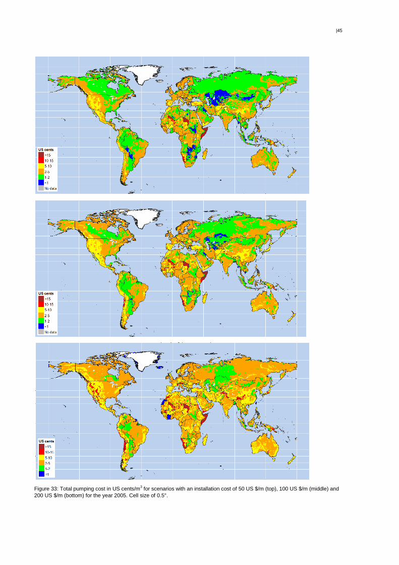
|45

Figure 33: Total pumping cost in US cents/m3 for scenarios with an installation cost of 50 US $/m (top), 100 US $/m (middle) and

200 US $/m (bottom) for the year 2005. Cell size of 0.5°.

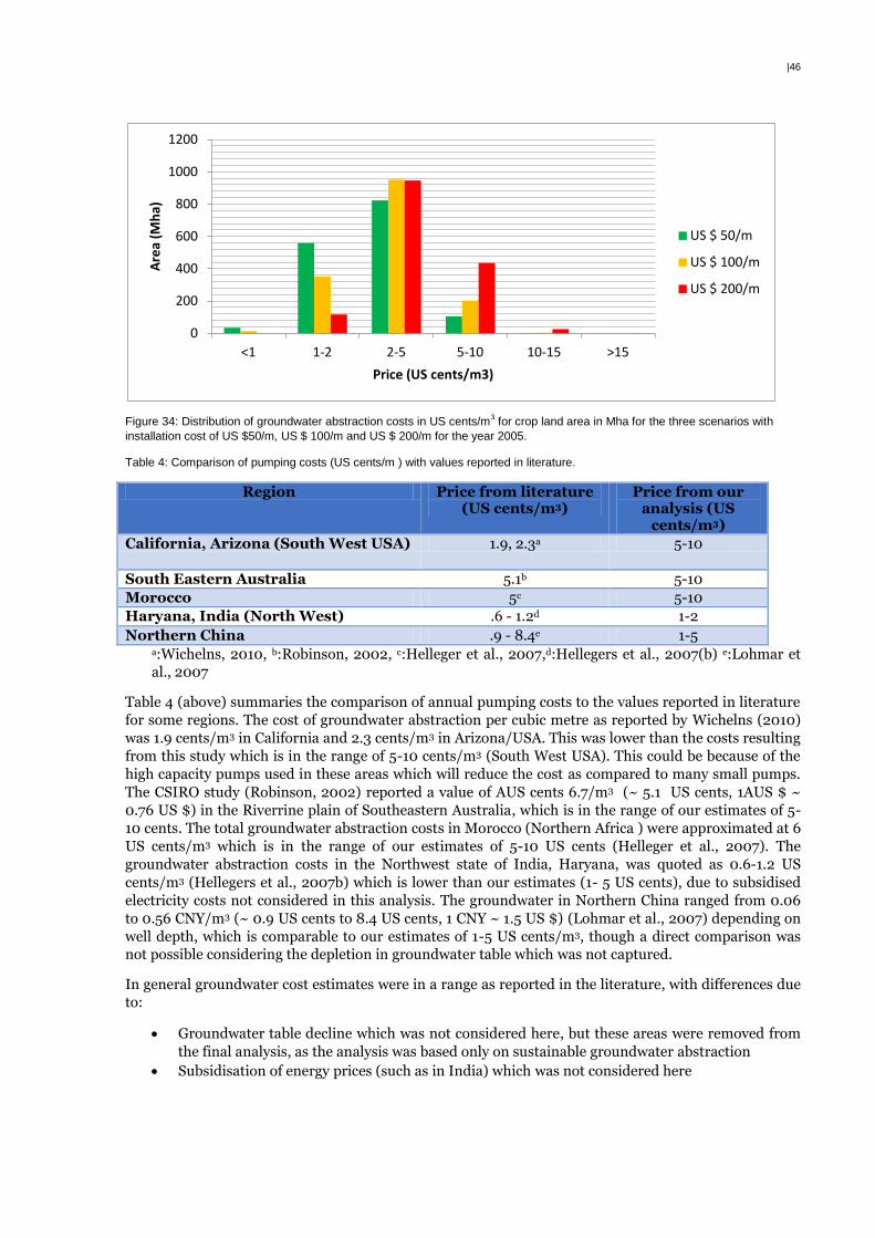
|46

Figure 34: Distribution of groundwater abstraction costs in US cents/m3 for crop land area in Mha for the three scenarios with

installation cost of US $50/m, US $ 100/m and US $ 200/m for the year 2005.

Table 4: Comparison of pumping costs (US cents/m ) with values reported in literature.

Region Price from literature (US cents/m3)

Price from our analysis (US

cents/m3)

California, Arizona (South West USA) 1.9, 2.3a 5-10

South Eastern Australia 5.1b 5-10

Morocco 5c 5-10

Haryana, India (North West) .6 - 1.2d 1-2

Northern China .9 - 8.4e 1-5 a:Wichelns, 2010, b:Robinson, 2002, c:Helleger et al., 2007,d:Hellegers et al., 2007(b) e:Lohmar et

al., 2007

Table 4 (above) summaries the comparison of annual pumping costs to the values reported in literature

for some regions. The cost of groundwater abstraction per cubic metre as reported by Wichelns (2010)

was 1.9 cents/m3 in California and 2.3 cents/m3 in Arizona/USA. This was lower than the costs resulting

from this study which is in the range of 5-10 cents/m3 (South West USA). This could be because of the

high capacity pumps used in these areas which will reduce the cost as compared to many small pumps.

The CSIRO study (Robinson, 2002) reported a value of AUS cents 6.7/m3 (~ 5.1 US cents, 1AUS $ ~

0.76 US $) in the Riverrine plain of Southeastern Australia, which is in the range of our estimates of 5-

10 cents. The total groundwater abstraction costs in Morocco (Northern Africa ) were approximated at 6

US cents/m3 which is in the range of our estimates of 5-10 US cents (Helleger et al., 2007). The

groundwater abstraction costs in the Northwest state of India, Haryana, was quoted as 0.6-1.2 US

cents/m3 (Hellegers et al., 2007b) which is lower than our estimates (1- 5 US cents), due to subsidised

electricity costs not considered in this analysis. The groundwater in Northern China ranged from 0.06

to 0.56 CNY/m3 (~ 0.9 US cents to 8.4 US cents, 1 CNY ~ 1.5 US $) (Lohmar et al., 2007) depending on

well depth, which is comparable to our estimates of 1-5 US cents/m3, though a direct comparison was

not possible considering the depletion in groundwater table which was not captured.

In general groundwater cost estimates were in a range as reported in the literature, with differences due

to:

Groundwater table decline which was not considered here, but these areas were removed from

the final analysis, as the analysis was based only on sustainable groundwater abstraction

Subsidisation of energy prices (such as in India) which was not considered here

0

200

400

600

800

1000

1200

<1 1-2 2-5 5-10 10-15 >15

Are

a (M

ha)

Price (US cents/m3)

US $ 50/m

US $ 100/m

US $ 200/m

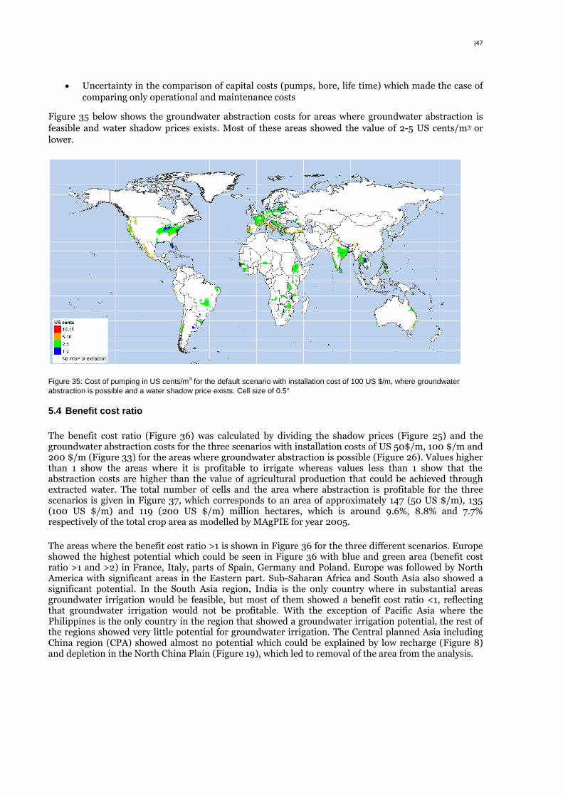
|47

Uncertainty in the comparison of capital costs (pumps, bore, life time) which made the case of

comparing only operational and maintenance costs

Figure 35 below shows the groundwater abstraction costs for areas where groundwater abstraction is

feasible and water shadow prices exists. Most of these areas showed the value of 2-5 US cents/m3 or

lower.

Figure 35: Cost of pumping in US cents/m3 for the default scenario with installation cost of 100 US $/m, where groundwater

abstraction is possible and a water shadow price exists. Cell size of 0.5°

5.4 Benefit cost ratio

The benefit cost ratio (Figure 36) was calculated by dividing the shadow prices (Figure 25) and the groundwater abstraction costs for the three scenarios with installation costs of US 50$/m, 100 $/m and 200 $/m (Figure 33) for the areas where groundwater abstraction is possible (Figure 26). Values higher than 1 show the areas where it is profitable to irrigate whereas values less than 1 show that the abstraction costs are higher than the value of agricultural production that could be achieved through extracted water. The total number of cells and the area where abstraction is profitable for the three scenarios is given in Figure 37, which corresponds to an area of approximately 147 (50 US $/m), 135 (100 US $/m) and 119 (200 US $/m) million hectares, which is around 9.6%, 8.8% and 7.7% respectively of the total crop area as modelled by MAgPIE for year 2005.

The areas where the benefit cost ratio >1 is shown in Figure 36 for the three different scenarios. Europe showed the highest potential which could be seen in Figure 36 with blue and green area (benefit cost ratio >1 and >2) in France, Italy, parts of Spain, Germany and Poland. Europe was followed by North America with significant areas in the Eastern part. Sub-Saharan Africa and South Asia also showed a significant potential. In the South Asia region, India is the only country where in substantial areas groundwater irrigation would be feasible, but most of them showed a benefit cost ratio <1, reflecting that groundwater irrigation would not be profitable. With the exception of Pacific Asia where the Philippines is the only country in the region that showed a groundwater irrigation potential, the rest of the regions showed very little potential for groundwater irrigation. The Central planned Asia including China region (CPA) showed almost no potential which could be explained by low recharge (Figure 8) and depletion in the North China Plain (Figure 19), which led to removal of the area from the analysis.

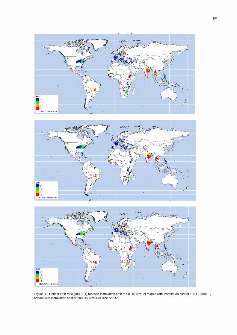
|48

Figure 36: Benefit cost ratio (BCR): 1) top with installation cost of 50 US $/m; 2) middle with installation cost of 100 US $/m; 3)

bottom with installation cost of 200 US $/m. Cell size of 0.5°.

|49

Figure 37: Area (Mha) and number of cells where BCR >1 for the three scenarios, with installation costs of 50 US $/m, 100 US

$/m and 200 US $/m.

Figure 38: Area (Mha) for the three installation cost scenarios for 10 MAgPIE regions. Sub-Saharan Africa (AFR), Centrally

Planned Asia Including China (CPA), Europe including Turkey (EUR), the newly independent states of the former soviet Union

(FSU), Latin America (LAM), Middle East/North Africa (MEA), North America (NAM), Pacific OECD including Japan, Australia,

New Zealand (PAO); Pacific Asia (PAS) and South Asia Including India (SAS).

5.4.1 Sensitivity to installation cost

The resulting difference in area from reducing the cost by 50% from 100 US $/m was moderate with an increase of 12 million hectares (8.8 %) of area with benefit cost ratio >1, whereas the effect of doubling the cost to 200 US $/m lead to a decrease of area to 16 million hectares (11.1 % of the total area). There are regional disparities between how the installation costs affected the benefit cost ratio with developing

2113

1899

1691

147 135 119

0

500

1000

1500

2000

2500

50 $/m 100$/m 200 $/m

Number of Cells Area (Mha)

0

10

20

30

40

50

60

AFR CPA EUR FSU LAM MEA NAM PAO PAS SAS

Are

a (M

ha)

Cost (US $/m)

Area (BCR>1)

50 $/m

100$/m

200 $/m

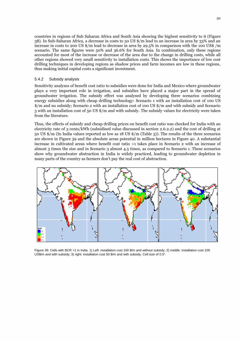
|50

countries in regions of Sub Saharan Africa and South Asia showing the highest sensitivity to it (Figure 38). In Sub-Saharan Africa, a decrease in costs to 50 US $/m lead to an increase in area by 33% and an increase in costs to 200 US $/m lead to decrease in area by 29.5% in comparison with the 100 US$ /m scenario. The same figures were 50% and 36.6% for South Asia. In combination, only these regions accounted for most of the increase or decrease of the area due to the change in drilling costs, while all other regions showed very small sensitivity to installation costs. This shows the importance of low cost drilling techniques in developing regions as shadow prices and farm incomes are low in these regions, thus making initial capital costs a significant investment.

5.4.2 Subsidy analysis

Sensitivity analyses of benefit cost ratio to subsidies were done for India and Mexico where groundwater

plays a very important role in irrigation, and subsidies have played a major part in the spread of

groundwater irrigation. The subsidy effect was analysed by developing three scenarios combining

energy subsidies along with cheap drilling technology: Scenario 1 with an installation cost of 100 US

$/m and no subsidy; Scenario 2 with an installation cost of 100 US $/m and with subsidy and Scenario

3 with an installation cost of 50 US $/m and with subsidy. The subsidy values for electricity were taken

from the literature.

Thus, the effects of subsidy and cheap drilling prices on benefit cost ratio was checked for India with an

electricity rate of 3 cents/kWh (subsidised value discussed in section 2.6.2.2) and the cost of drilling at

50 US $/m (In India values reported as low as 18 US $/m (Table 3)). The results of the three scenarios

are shown in Figure 39 and the absolute areas potential in million hectares in Figure 40. A substantial

increase in cultivated areas where benefit cost ratio >1 takes place in Scenario 2 with an increase of

almost 3 times the size and in Scenario 3 almost 4.5 times, as compared to Scenario 1. These scenarios

show why groundwater abstraction in India is widely practiced, leading to groundwater depletion in

many parts of the country as farmers don’t pay the real cost of abstraction.

Figure 39: Cells with BCR >1 in India. 1) Left: installation cost 100 $/m and without subsidy; 2) middle: installation cost 100

US$/m and with subsidy; 3) right: installation cost 50 $/m and with subsidy. Cell size of 0.5°.

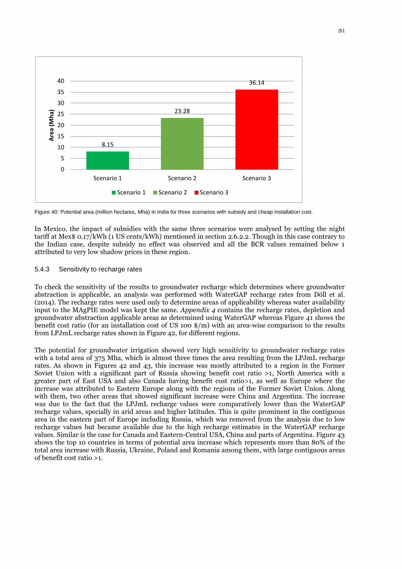
|51

Figure 40: Potential area (million hectares, Mha) in India for three scenarios with subsidy and cheap installation cost.

In Mexico, the impact of subsidies with the same three scenarios were analysed by setting the night tariff at Mex$ 0.17/kWh (1 US cents/kWh) mentioned in section 2.6.2.2. Though in this case contrary to the Indian case, despite subsidy no effect was observed and all the BCR values remained below 1 attributed to very low shadow prices in these region.

5.4.3 Sensitivity to recharge rates

To check the sensitivity of the results to groundwater recharge which determines where groundwater abstraction is applicable, an analysis was performed with WaterGAP recharge rates from Döll et al. (2014). The recharge rates were used only to determine areas of applicability whereas water availability input to the MAgPIE model was kept the same. Appendix 4 contains the recharge rates, depletion and groundwater abstraction applicable areas as determined using WaterGAP whereas Figure 41 shows the benefit cost ratio (for an installation cost of US 100 $/m) with an area-wise comparison to the results from LPJmL recharge rates shown in Figure 42, for different regions.

The potential for groundwater irrigation showed very high sensitivity to groundwater recharge rates with a total area of 375 Mha, which is almost three times the area resulting from the LPJmL recharge rates. As shown in Figures 42 and 43, this increase was mostly attributed to a region in the Former Soviet Union with a significant part of Russia showing benefit cost ratio >1, North America with a greater part of East USA and also Canada having benefit cost ratio>1, as well as Europe where the increase was attributed to Eastern Europe along with the regions of the Former Soviet Union. Along with them, two other areas that showed significant increase were China and Argentina. The increase was due to the fact that the LPJmL recharge values were comparatively lower than the WaterGAP recharge values, specially in arid areas and higher latitudes. This is quite prominent in the contiguous area in the eastern part of Europe including Russia, which was removed from the analysis due to low recharge values but became available due to the high recharge estimates in the WaterGAP recharge values. Similar is the case for Canada and Eastern-Central USA, China and parts of Argentina. Figure 43 shows the top 10 countries in terms of potential area increase which represents more than 80% of the total area increase with Russia, Ukraine, Poland and Romania among them, with large contiguous areas of benefit cost ratio >1.

8.15

23.28

36.14

0

5

10

15

20

25

30

35

40

Scenario 1 Scenario 2 Scenario 3

Are

a (M

ha)

Scenario 1 Scenario 2 Scenario 3

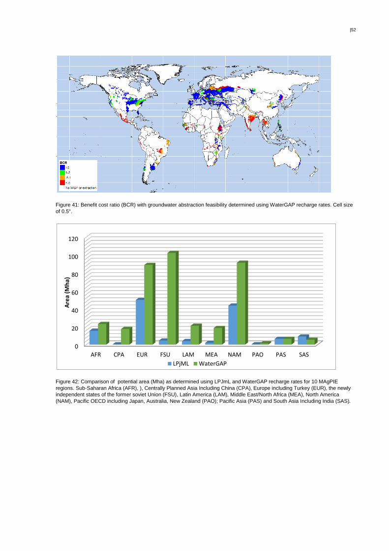
|52

Figure 41: Benefit cost ratio (BCR) with groundwater abstraction feasibility determined using WaterGAP recharge rates. Cell size

of 0.5°.

Figure 42: Comparison of potential area (Mha) as determined using LPJmL and WaterGAP recharge rates for 10 MAgPIE

regions. Sub-Saharan Africa (AFR), ), Centrally Planned Asia Including China (CPA), Europe including Turkey (EUR), the newly

independent states of the former soviet Union (FSU), Latin America (LAM), Middle East/North Africa (MEA), North America

(NAM), Pacific OECD including Japan, Australia, New Zealand (PAO); Pacific Asia (PAS) and South Asia Including India (SAS).

0

20

40

60

80

100

120

AFR CPA EUR FSU LAM MEA NAM PAO PAS SAS

Are

a (M

ha)

LPjML WaterGAP

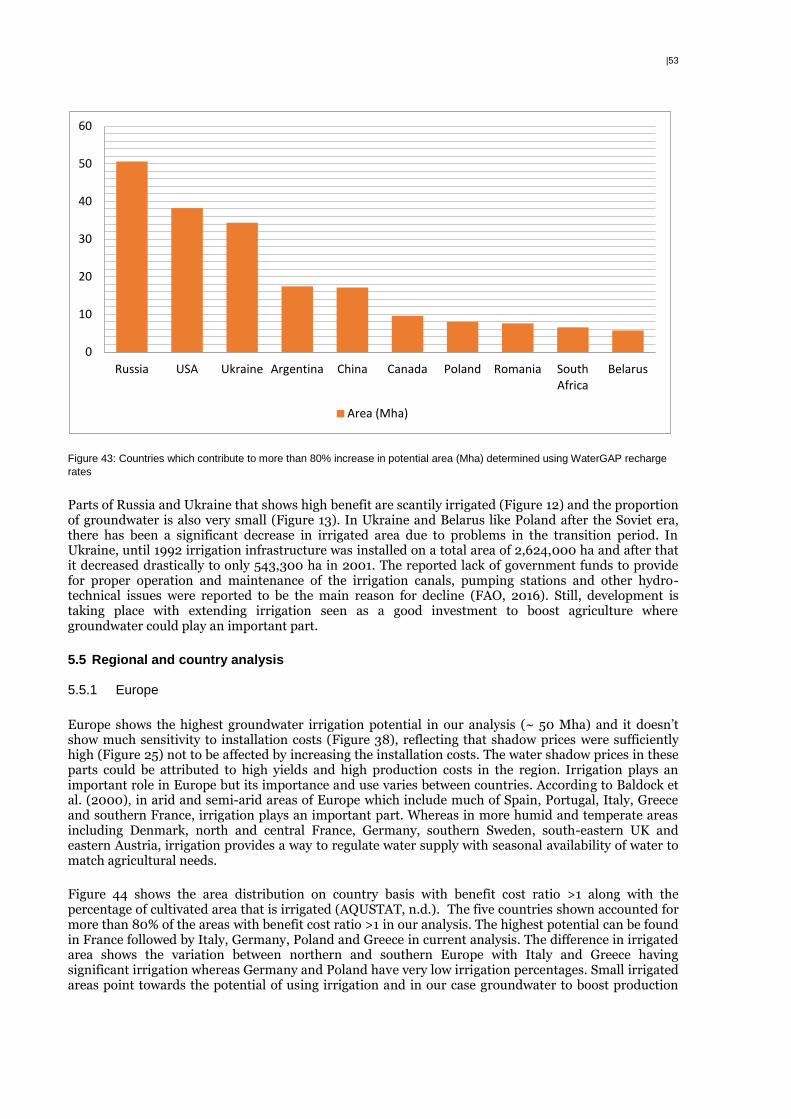
|53

Figure 43: Countries which contribute to more than 80% increase in potential area (Mha) determined using WaterGAP recharge

rates

Parts of Russia and Ukraine that shows high benefit are scantily irrigated (Figure 12) and the proportion of groundwater is also very small (Figure 13). In Ukraine and Belarus like Poland after the Soviet era, there has been a significant decrease in irrigated area due to problems in the transition period. In Ukraine, until 1992 irrigation infrastructure was installed on a total area of 2,624,000 ha and after that it decreased drastically to only 543,300 ha in 2001. The reported lack of government funds to provide for proper operation and maintenance of the irrigation canals, pumping stations and other hydro-technical issues were reported to be the main reason for decline (FAO, 2016). Still, development is taking place with extending irrigation seen as a good investment to boost agriculture where groundwater could play an important part.

5.5 Regional and country analysis

5.5.1 Europe

Europe shows the highest groundwater irrigation potential in our analysis (~ 50 Mha) and it doesn’t show much sensitivity to installation costs (Figure 38), reflecting that shadow prices were sufficiently high (Figure 25) not to be affected by increasing the installation costs. The water shadow prices in these parts could be attributed to high yields and high production costs in the region. Irrigation plays an important role in Europe but its importance and use varies between countries. According to Baldock et al. (2000), in arid and semi-arid areas of Europe which include much of Spain, Portugal, Italy, Greece and southern France, irrigation plays an important part. Whereas in more humid and temperate areas including Denmark, north and central France, Germany, southern Sweden, south-eastern UK and eastern Austria, irrigation provides a way to regulate water supply with seasonal availability of water to match agricultural needs.

Figure 44 shows the area distribution on country basis with benefit cost ratio >1 along with the percentage of cultivated area that is irrigated (AQUSTAT, n.d.). The five countries shown accounted for more than 80% of the areas with benefit cost ratio >1 in our analysis. The highest potential can be found in France followed by Italy, Germany, Poland and Greece in current analysis. The difference in irrigated area shows the variation between northern and southern Europe with Italy and Greece having significant irrigation whereas Germany and Poland have very low irrigation percentages. Small irrigated areas point towards the potential of using irrigation and in our case groundwater to boost production

0

10

20

30

40

50

60

Russia USA Ukraine Argentina China Canada Poland Romania South Africa

Belarus

Area (Mha)

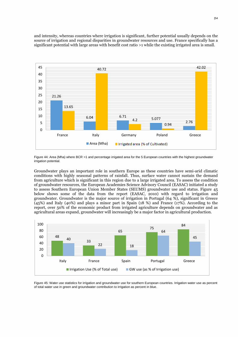
|54

and intensity, whereas countries where irrigation is significant, further potential usually depends on the source of irrigation and regional disparities in groundwater resources and use. France specifically has a significant potential with large areas with benefit cost ratio >1 while the existing irrigated area is small.

Figure 44: Area (Mha) where BCR >1 and percentage irrigated area for the 5 European countries with the highest groundwater

irrigation potential.

Groundwater plays an important role in southern Europe as these countries have semi-arid climatic conditions with highly seasonal patterns of rainfall. Thus, surface water cannot sustain the demand from agriculture which is significant in this region due to a large irrigated area. To assess the condition of groundwater resources, the European Academies Science Advisory Council (EASAC) initiated a study to assess Southern European Union Member States (SEUMS) groundwater use and status. Figure 45 below shows some of the data from the report (EASAC, 2010) with regard to irrigation and groundwater. Groundwater is the major source of irrigation in Portugal (64 %), significant in Greece (45%) and Italy (40%) and plays a minor part in Spain (18 %) and France (17%). According to the report, over 50% of the economic product from irrigated agriculture depends on groundwater and as agricultural areas expand, groundwater will increasingly be a major factor in agricultural production.

Figure 45: Water use statistics for irrigation and groundwater use for southern European countries. Irrigation water use as percent

of total water use in green and groundwater contribution to irrigation as percent in blue.

21.26

6.04 6.71 5.077

2.76

13.65

40.72

4.2 0.94

42.02

0

5

10

15

20

25

30

35

40

45

France Italy Germany Poland Greece

Area (Mha) Irrgated Area (% of Cultivated)

48 33

65 75

84

40

22 18

64

45

0

20

40

60

80

100

Italy France Spain Portugal Greece

Irrigation Use (% of Total use) GW use (as % of Irrigation use)

|55

According to the EASAC country report on France (Barraqué et al., 2010), irrigation water which is of major importance mostly comes from surface water in the southern part, whereas in the north irrigation is provided mainly by groundwater with values above 90% in the Artois-Picardie, Rhine-Meuse, and Seine-Normandie hydrographic basins in northern and eastern France. In France, both groundwater quantity and quality problems exist for groundwater with diffuse pollution from agriculture and there are several cases of aquifer overexploitation such as the Beauce aquifer in central France (in Figure 19 represented as depleted, removed from the our analysis). According to the report, among the 553 groundwater bodies analysed for the water framework directive, 216 were identified to be at risk of not reaching good environmental status in 2015, and 100 doubtful ones for both qualitative and quantitative reasons. In France, the annual volume abstracted from groundwater reserves is approximately 6 billion m3 which is much smaller than the estimated recharge of 100 billion m3, thus in terms of quantity, the risk of water shortages is relatively negligible at national scale (Blum, 2004). Therefore, France holds a significant potential for further groundwater use in irrigation as supported by our analysis, however due to considerable differences between regions, more region specific studies are required considering the existing quantity and quality problems in several aquifers.

In Italy, groundwater irrigation is more developed than in France and plays an important role, with a groundwater irrigation area of 89,565 ha 2010 (41% of the total irrigated area). The estimated groundwater abstraction for irrigation is pegged at 6.97 billion m3 in 2010 (OECD, 2015 compared to the estimated annual renewable groundwater of 12.1 billion m3 reported by the EASAC country groundwater report on Italy (Civita et al., 2010) from different sources. According to these authors, there is a great variability in different parts of Italy with renewable groundwater sources decreasing as we move from the more humid northern parts (53.7%) to the semi-arid southern parts (15.7%). In contrast, groundwater resources contribution to the total water resource increase as we move south, estimated to 78%, 52 % and 96% in the northern, central and southern parts, respectively. Overexploitation of ground water exists in many parts of the Italian territory, mostly in densely populated areas and in plain and coastal regions as well as in densely cultivated areas, most notably the Po valley in the northern part (represented in Figure 19 as depleted area and thus removed from the our analysis). Therefore, as is the case with France, more region specific studies would be required to ascertain the true potential considering the uneven distribution between regions with quantity and quality problems in several parts.

Northern Europe differs from southern Europe regarding the fact that agriculture is mainly rainfed, but the benefit cost ratio in our analysis shows that groundwater irrigation would be beneficial considering the high yields that could be achieved in the region. Germany and Poland show very high potential for groundwater irrigation in our anlaysis due to ample recharge and low irrigated area at present. The irrigation in both these countries is only supplementary and applied during dry periods or drought, but increasing in importance owing to the risks posed by increased cases of longer dry periods and more frequent droughts.

Poland along with many Central and Eastern European Countries (CEEW), after the transition period from the Soviet Union era starting in early 1990s, saw a steep reduction in irrigated area from 301,500 ha in 1990 to just 83,300 ha in 2003. It was due to problems of privatisation and management transfer as centrally planned large-scale irrigation infrastructure were less adapted to the new private landownership and land parcelling as well as to the new (high) prices for energy and materials, thus irrigation dropped significantly (Zhovtonog et al., 2005). Irrigation at present has not recovered and irrigated area accounts for a very small percent of agricultural land (Figure 15). According to Łabedzki (2009), irrigation in Poland is of a supplementary character being used in short periods during the growing season, especially in regions with severe and frequent droughts, whereas in wet years the role of irrigation is marginal, except for fruit and vegetable farming where irrigation is essential every year. According to the author, irrigation will play an important role in mitigating the effects of drought on crop production and effects of climate change may boost water demand in agriculture by 30–50% in the next 20–30 years, with much of this increased demand due to more need from irrigated agriculture. According to the OECD report (OECD, 2015), Poland uses virtually no groundwater for irrigation which can be accounted to the low irrigation level in the country, thus providing a total untapped potential. After becoming an EU member, the value of agriculture exports has increased fivefold, from EUR 4 billion in 2004 to 21.3 billion in 2014. Furthermore, there has been a 25 per cent decrease in the number of the smallest farms (0–5 ha of agricultural area) and a 34 per cent increase in the number of

|56

the largest farms (50 ha and more) (Kolodziejczyk, 2016), which indicates the growth in agriculture towards larger farms that could lead to more irrigation infrastructure. Three main factors that will play an important part on the development of irrigation are: increased frequency and intensity of droughts; the intensification of agricultural production (e.g. in horticulture, orchards, seed crops) being forced by the domestic and European free-market competition and the necessity of obtaining high quality of the agricultural products (Łabedzki, 2009). Thus, groundwater in Poland presents a significant and valuable source, reflected in high benefit cost ratio values in our analysis, which can play an important part in irrigation expansion to increase agricultural production, increase crop intensity and adaptation to climate change.

In Germany, the agricultural area is significant at approximately 17 million hectares but similar to Poland, irrigation only plays a supplementary role during dry periods in the growing season, with only 4.2 % of the agricultural area irrigated and agricultural water withdrawals accounting for less than 0.5 % of the total water withdrawals. Still, groundwater plays a significant role in this limited irrigation with 82 % of the irrigated area quipped with groundwater irrigation (AQUASTAT, n.d.). The irrigation methods employed are mainly sprinkler systems, for which generally groundwater is extracted. Groundwater abstraction in quantity is dominated by domestic drinking water supply with over two-thirds of the population relying on it. Total groundwater extracted in 2010 was 5.84 km³, mostly for drinking water supply (3.53 km3) and a very small part of 0.22 km3 for industrial sectors including agriculture accounts only for approximately 12% of the annual groundwater recharge in Germany, which has been estimated at 48.2 km³ (BGR, n.d.).

Thus, due to ample recharge and low irrigated area similar to Poland, Germany has a high potential to extend irrigation as a way to make agriculture resilient to dry periods and droughts. Groundwater can play an important role in adapting to future climate change, which is expected to increase the severity of drought periods and aggravate resource pressures in many regions of Europe. Particular crises in water availability are predicted for Spain, but also including France, the UK and Germany, potentially driving a greater economic need for irrigation (Baldock, et al., 2000). Thus, to improve water retention and irrigation infrastructures where agricultural and forest landscapes are threatened by drought is the measure recommended in the Germany national strategy for adaptation to climate change (BMU, 2009).

So both Germany and Poland show groundwater irrigation potential as corroborated by our analysis and literature but here the use of groundwater would be more supplementary, in contrast to southern Europe where irrigation is necessary. Groundwater irrigation could play an important role in building resilience and adapting to climate change, which could make rainfall more seasonal, thus exacerbating dry periods and could lead to more frequent droughts which will limit the surface water supply. But there is a need for careful planning to not overexploit groundwater which is the case in many southern European countries and also to protect it from nutrients pollution prevalent over all over Europe due to high use of fertilisers.

5.5.2 North America

In our analysis, North America and especially eastern USA showed high groundwater irrigation potential (~ 43.4 Mha) with most of the area having benefit cost ratio >1 and majority of it having benefit cost ratio >2. This was driven by high shadow prices which were though lower than the Central Plains and the Western States (Figure 25) but still higher than many other parts of the world. Aquifers in this region are mainly characterized by complex hydro-geological structures and carbonate aquifers as shown in Figure 24. Many of these complexes of hydro-geological structures consist of sandstone aquifers with of low to moderate groundwater yields (hydraulic conductivity), but because they extend over large areas, these aquifers provide large volumes of water (UNESCO, 2004). Carbonate aquifers shows highly variable yields as water is transmitted through cracks and fractures with areas of high yield in close proximity to low yield areas. Thus, eastern USA contains a high potential for groundwater development but the hydrogeology is complex which would need careful studies before installing wells.

Other than the potential groundwater sources, eastern USA shows high potential for groundwater development as irrigated areas in this part are comparatively smaller compared to the more arid central

|57

and western states (Figure 15). There, groundwater is extensively used as farmers commonly rely heavily on frequent summer rainfall to meet crop water needs. In USA, 7.6 percent of all cropland and pastureland were irrigated in 2012 with nearly 75% of the irrigated area in the 17 western-most states, which also contributed to 80% of the irrigated water withdrawals that accounts for 38% of the nation's freshwater withdrawals in 2010 (Schaible & Aillery, 2015). Groundwater withdrawals for irrigation have peaked or decreased in the western states in recent decades as a result of expanding urban areas, an increase in dryland farming, and increased efficiencies of application.

Due to the favourable conditions and untapped potential, ground-water withdrawals for irrigation in the eastern half of the country have increased steadily from approximately 2000 MGD (million gallon per day, 1000 MGD = 3.78 million m3/day) in 1960 to around 15000 MGD in 2000 as a supplemental source of water to protect against dry periods as reported by U.S. Geological Survey (Reilly et al., 2008). Irrigation is becoming more common in these regions as reported by (Levin & Zarriello, 2013), with the acreage of irrigated land in New England increasing by 3 percent from 2003 to 2008. In the mid-Atlantic region, irrigated acreage increased by 33 percent during this time. Both the regions are located in the eastern USA. The eastern USA region is more humid with higher recharge rates than the central and south-western parts (Figure 8), thus providing ample resources for development which are still untapped. This could be compared to the western and central parts which have undergone depletion. Thus, the high benefit cost ratio in our analysis reflects the potential for groundwater irrigation in eastern USA which is still not completely developed.

5.5.3 Sub-Saharan Africa

In our analysis, Sub-Saharan Africa, the southern and eastern countries of Zimbabwe, Kenya, Malawi, Tanzania, Ethiopia and some parts of South Africa show benefit cost ratio >1. In these areas, irrigation is scant and groundwater development is less as seen in Figures 15 and 16, thus they show to be potential areas of future renewable groundwater development for irrigation. Agriculture in Sub-Saharan Africa is mostly rainfed and limited access to water in arid areas or during dry seasons or droughts is a restricting factor for farming and for improving agricultural productivity (Xie et al., 2014). Groundwater irrigation covers only 1% of the cultivated land whereas the same figure stands at 14% for Asia (Siebert, et al., 2010), showing the potential for further development of irrigation. Unlike Asia where groundwater over-abstraction is the problem, a Sub-Saharan Africa problem is generally one of underdevelopment and the region has missed both the green and groundwater revolutions, being the only major region in which per capita food production has actually declined over the last 30 years (Giordano, 2006). Owing to these reasons, studies estimating the groundwater irrigation potential have been done in Sub-Saharan Africa.

Altchenko and Villholth (2015) calculated the potential of renewable groundwater for irrigation in Africa and concluded that the eastern part of Africa from Ethiopia to Zimbabwe may provide significant groundwater development opportunities for irrigation. They estimated the total groundwater irrigation potential to be 44.6 Mha to 105.3 Mha for different environmental flow scenarios, though their estimates were just based on groundwater availability and they didn’t consider any cost factor. Xie et al. (2014) in their study estimated the small-holder irrigation potential in Sub-Saharan Africa using a cost-benefit analysis with irrigation and production costs for motor pumps, treadle pumps, communal river diversion, and small reservoirs. Their results indicated a large potential for the expansion of smallholder irrigation in Sub-Saharan Africa with 30 million ha for motor pumps, followed by 24 million ha for treadle pumps, 22 million ha for small reservoirs and 20 million ha for communal river diversions. With respect to the above, the estimated value area in the current analysis, where benefit cost ratio >1, varied from 10.91 Mha (with a cost of 200 US $/m) to 20.7 Mha (with a cost of 50 US $/m) which is less than both the above estimates. The difference from the first estimate could be attributed to the reason that it reflects only the potential based solely on water availability without considering any cost-benefit analysis. The estimates of the second study which did consider the cost-benefit analysis could be attributed to different recharge estimates, different criteria chosen for applicability where a limit of minimum 20 mm was used, while they used no such limitation. In addition, they used a different model and way to analyse the costs and benefits associated with irrigation. Where the current study used groundwater table depth, electricity and pump prices to drive the spatially explicit groundwater abstraction costs they used a single estimate for the entire region.

|58

Though most of the studies have focused on potential of irrigation through groundwater by considering recharge only (Xie et al. (2014), Altchenko and Villholth (2015) ), the groundwater yields also play an important role. The area where benefit cost ratio >1 is mostly categorised as having local and shallow aquifers and complex hydro-geological structures, with yields that can differ widely between areas. MacDonald et al. (2012) estimated the yields in Africa and found that aquifers supporting yields of more than 5 l/s were not widespread, with a majority of aquifers yielding 0.1 to 5l/s. The current study used a yield of 5l/s for pumping though small scale irrigation could be done with lower yields, but would not be possible in very low yields, and thus acts as a limitation. The current results showed the uncertainty and sensitivity of potential irrigation estimates based on different studies and factors, but nonetheless confirmed the previous results that substantial potential does exists in the Sub-Saharan Africa region, for groundwater development for irrigation. Owing to this potential, several projects focussing on understanding and developing groundwater in Sub-Saharan has been carried out, such as Groundwater in Sub-Saharan Africa by IWMI (http://gw-africa.iwmi.org/) and Groundwater Futures in Sub-Saharan Africa (GroFutures, https://upgro.org/) funded by the UK Department for International Development (DFID).

5.5.4 South Asia and Centrally planned Asia including China

In South Asia and the North China plain, groundwater is the main source of irrigated agriculture with India, Pakistan, Bangladesh and North China using over 300-400 km3 of groundwater annually, which is near half of the world’s total annual use (Shah, 2007). Despite the importance of groundwater and significant abstractions, the current analysis show very limited groundwater irrigation potential (South Asia = 9 Mha, China = 0.25 Mha). There are three main reasons for this; firstly, the main groundwater abstraction areas of India (the north-west part and the southern Peninsula), China (North China plain), Pakistan (the north east part) are already over-extracted and depleted (Figure 19) and therefore they were removed from the analyses. Secondly, the recharge was low (Figure 8) in higher latitudes which removed much of Chinese area from the analysis where a water shadow price exists (Figure 25). Thirdly, there are very low water shadow prices in parts of India where the groundwater abstraction was still feasible but the benefit cost ratio was less than one. Thus, they in combination made most of the areas not suitable for groundwater abstraction or unprofitable, but still India shows a significant area where abstraction would be profitable.

The reason that despite widespread groundwater depletion problems in India, a substantial area with abstraction potential exists, is because of the intra-regional disparity of groundwater development. Groundwater irrigation contributes significantly in the country in the north western parts and in the Southern Peninsula region such as Punjab, Western Uttar Pradesh, Gujarat, and Tamil Nadu, which are already overexploiting the groundwater. On the other hand, in the eastern parts of the country, the level of groundwater development is very low. Overall, only 31 per cent of the known groundwater potential is estimated to be developed in the eastern states, though accounting for more than 55 per cent of India's net irrigated area (Srivastava et al. 2013). The north west, most of the Indo-Gangetic plain and the Southern Peninsula, where most of the groundwater abstraction takes place, were removed in the current analysis as these areas are already highly exploited. In the areas where benefit was less than one, irrigation was less dense (Figure 15) and use of groundwater was also less (Figure 16), as compared to the north west and the Southern Peninsula of India. These parts cover the Indian States of West Bengal, Bihar, Odisha, Chhattisgarh and Madhya Pradesh, where agriculture exists but groundwater development is low. This is due to the combination of poverty, low electrification rates, difficulty in obtaining electricity connections for electric pumps and increasing diesel prices. The Central Ground Water Board (CGWB) of India in their annual report of 2013-2014 reported the groundwater development percent at 44% for Bihar, 35% for Chattisgarh, 57% for Madhya Pradesh, 40% for West Bengal and 28% for Odisha, showing the potential available in these areas for groundwater irrigation development (CGWB, 2015).

The existing use of groundwater in India in these regions, although relatively much lower than other parts, and despite low shadow prices which lead to benefit cost ratio <1, could be explained by the high energy subsidies provided by the government for Indian agriculture and cheap drilling techniques. In the Indian electricity market, the agricultural prices are less than half the rate charged to industrial and commercial users and in many parts are fixed rates based on pump horsepower. Agricultural electricity subsidies act as a tool to increase agricultural production through enhanced groundwater irrigation, and

|59

in doing so aim to benefit poor rural households and stabilize food prices (Badiani & Jessoe, 2010). During 1971-2009, the total electricity consumption in India increased 12-fold but increases in estimated agricultural electricity consumption were more than double of that to about 25-fold (Gulati & Pahuja, 2015). As stated in Section 2.6.2.2, power subsidies for the agricultural sector is estimated at US$ 6 billion a year — two and a half times the yearly expenditure on irrigation (Monari, 2002).

The effect of subsidies and cheap drilling prices on the benefit cost ratio for India in current analysis, with an electricity rate of INR 2/kWh (~3 cents/kWh) and cost of drilling at 50 US $/m (Figures 39 and 40), shows that subsidies have contributed significantly in making groundwater abstraction affordable. This has made groundwater use for irrigation widely acceptable, which in turn has led to groundwater depletion in many parts as farmers do not pay the real cost of abstraction. Thus it has remained beneficial despite the low shadow prices. Still small parts of coastal Orissa (on the central west coast), Madhya Pradesh (central) and Western Ghats (mountain region) show benefit cost ratio <1, reflecting that even after subsidies, groundwater abstraction remains unprofitable. The existence of subsidies is a debatable issue, where on one side it helps small scale farmers which form the majority in India to sustain incomes, but at the same time it leads to over-exploitation of groundwater as there is no cost attached to it, and high losses to electricity boards in India which manifests itself in low and unreliable electricity supply. Thus, the current analysis shows the potential of groundwater irrigation in eastern India but it is profitable only with subsidies, thus necessitating a sustainable development approach so that these states do not follow the path of the north west states of India where extensive groundwater depletion is taking place. Also, risk of irrigation induced salinization as discussed in section 2.4 has to be considered in India since many parts fall into arid and semi-arid climate zone.

5.5.5 Pacific Asia

In Pacific Asia, groundwater recharge is abundant (Figure 8) but the irrigation is mostly rainfed and dependent upon surface water resources due to ample rainfall. Still, significant groundwater irrigation potential exists in Philippines in (6.38 Mha) whereas in Thailand all benefit cost ratio values are less than one showing that increase in the value of the yield with additional water is limited here.

In Philippines, agriculture is an important part of the economy with 70 percent of the country’s poor coming from rural areas, where agriculture is the dominant source of livelihood, and employment contributing to 37 percent of the jobs and 20 percent of the GDP of the country (Habito & Briones, 2005). In the Philippines, 18.26% of the cultivated area is equipped for irrigation of which just 5.6% are equipped for groundwater irrigation. Agricultural water withdrawals account for 83% of the total water withdrawals estimated for the year 2006 (AQUASTAT, n.d.), thus reflecting that rainfed agriculture is prominent and surface water is the main source of irrigation. Despite ample rainfall, benefit cost ratio >1 shows that there is a potential to increase yields through expansion of irrigation here, by tapping into groundwater resources.

The Philippines Institute Development Studies did a study (Inocencio et al., 2016) to assess the National Irrigation Schemes (NIS) and Communal Irrigation Schemes (CIS) managed by the National Irrigation Administration (NIA). According to the study, in both NIS (area >1000 ha) and CIS (area <1000 ha) groundwater pump systems contributed a very small part. According to the study, at least 90% of the pump irrigation used by rice farmers had been purchased privately. They found that pump systems were more successful due to their adequate water supply even during dry seasons, fewer problems occurred as compared to irrigation canals and structures which faced more severe water shortages, and greater incidences of funding problems and water theft. They concluded that groundwater remains a viable option for areas where the surface water sources have low dependable discharges during the dry seasons, and are underlain by high quality shallow aquifers. Here, groundwater is reliable even in intense drought periods or El Niño episodes, and farmers have control of irrigation schedules and flows despite extra costs of fuel and operation. Nevertheless, assessments on policy, discounts, dependable flows, catchment conditions, sediment discharges and potential of groundwater sources should be properly carried out before engaging in any scheme.

Thus, the groundwater potential in Philippines provides a viable option to expand irrigation and irrigation intensity especially in the dry months to ensure year round water supply. NIA has been

|60

implementing new groundwater projects in Central Luzon with an area of 3900 ha and in the TARLAC groundwater irrigation project with 3020 ha to boost agricultural production and farm income, and catalyze agro-industrial development in the region (National Irrigation Administration, n.d.). Considering the potential, more individual and small scale groundwater irrigation projects would also be a good option, considering the large funding required in developing these big projects.

In Thailand, agriculture is an important part of the economy with around 50% of the active population in this sector and contributing to 10% of the Thai gross domestic product. Irrigation is well developed (Figure 15) but the contribution of groundwater irrigation to the overall irrigated land is small (Figure 16), with surface water being the main resource due to ample rainfall and many surface irrigation projects. This is reflected in the shadow price which is very low, thus causing the benefit cost ratio to be less than 1. But groundwater is becoming more important to be used as supplementary irrigation in cases where there is insufficient supply from surface water. This is due to water shortages during the droughts and dry spells in the rainy season as well as in the dry season in many areas (Kwanyuen et al., 2003). In the Chao Phraya basin, the typical dry-season shortfall in supply from surface water and increased demand for dry season cultivation of high-value crops, led to explosive groundwater development with more than 10,000 wells being developed in a short period of time (Foster, 2008, FAO, 2013). There is no tax reduction or subsidy policy for individual farmers regarding electricity charges (Kwanyuen et al., 2003). Thus, shadow prices here reflect the average over long term which is low due to abundant surface water, but dry spells and droughts during which surface water is not sufficient can make the use of groundwater resources beneficial, which is reflected in the increased use of groundwater for irrigation over the last 10 years. Thus, long term climate impacts on water availability in Thailand will play a big role on the development of groundwater irrigation.

5.5.6 Latin America

In Latin America, Mexico is the country where groundwater use in irrigation is highest (Figure 15) and this has even led to groundwater depletion in many parts (Figure 19). Despite extensive groundwater use and an arid climate, the benefit cost ratio in our analysis in Mexico is very low which can be attributed to both very low shadow prices (Figure 25) and comparatively higher abstraction prices (Figure 33) due to deep groundwater tables (Figure 23). In Mexico, similar to India, electricity subsidies for pumping play a big role, with agricultural prices at the lowest and an estimated net subsidy of US$ 6 billion per year (CEE/ITESM, 2006). Electricity for groundwater pumping is subsidized by a factor of two to four times compared to the commercial rates .To analyse the impact of subsidies, a subsidy analysis was done with night electricity tariff as reported in the literature discussed in section 2.6.2.2, but contrary to Indian case no effect was found. This could be partly attributed to high abstraction and low shadow prices but also due to the fact that the area of Central Mexico which is a main agricultural production area was removed from our analysis as it is already depleted.

In South America, the benefit cost ratio was only positive in Argentina and Chile where the climate is more arid, whereas in Brazil the benefit cost ratio was less than 1. The highest potential of groundwater irrigation in crop land area was found in Chile with 1.59 Mha and Argentina with 2.07 Mha, whereas Brazil had almost no area (0.25 Mha) with benefit cost ratio >1, with most cells showing a value between 0.5 to 1. The small groundwater irrigation development could be attributed to an ample rainfall with an annual average between 1,000 and 2,000 mm. The Amazon rain forest and most of Central America receives an annual average precipitation between 2,000 to 4,000 mm, thus the river flows constitute the bulk of the usable surface water in most countries, and have been the main source of water supply (UNESCO, 2004). This was reflected in the shadow prices of our analysis which existed only in some parts of north eastern Brazil, north eastern and central Argentina and on the western coast with the Andes in Chile where rainfall is lesser.

The part where the benefit cost ratio was greater than 1 in Argentina is part of the Pampa plains and the north east region that are important for agricultural and cattle production. Ninety percent of the agricultural land in the Argentine Pampa is used for production of soybeans followed by wheat, maize and sunflowers (Galindo, et al., 2007). This region is already used for irrigation but also faces salinity problems, enhanced by extremely low topographic gradients existing in the region, usually lower than

|61

0.1 % (Romanelli et al., 2012). With the area still sparsely irrigated, this part presents a good potential for further groundwater development.

In Chile, the majority of the area where the benefit cost ratio >1 was located in the central valley which is in the central-south part along the Andes. This formation has been developed under the influence of glaciers and alluvial events with a considerable range of different soils constituting the main basis of agricultural activities in the country (Vera, 2013). The central valley mostly relies on surface water with canals and reservoirs built providing water during dryer months. Climate change impacts are projected to lead to reduction in annual precipitation by more than 30% in some areas of the country by 2040, and central Chile, where 70% of the total population lives, may see a significant reduction in precipitation (OECD, 2013). Thus, groundwater could provide an important buffer and potential during dry periods but its availability needs to be understood in conjunction with extensive surface irrigation network.

Other areas where the benefit cost ratio >1 was distributed across regions in various countries as in the south and north east coast of Australia, Belarus and some parts of westernmost Russia where groundwater irrigation potential exists and could be explored.

5.6 Synthesis

The results showed that significant potential exists for groundwater abstraction to expand irrigation which can help in increasing agricultural production. This groundwater irrigation potential not only exists in areas where precipitation and surface water sources are limited or seasonal as in Africa or India but also in more humid areas of northern Europe and Pacific Asia. Another factor which differentiates the areas of groundwater irrigation potential is low development and need of irrigation. Areas in Sub-Saharan Africa and Eastern India are areas where irrigation is required due to low or seasonal rainfall but groundwater development is low because of factors related to cost of development and knowledge of groundwater resources. In these areas, factors that could reduce the cost of abstraction such as subsidies and cheap drilling techniques are important to make groundwater use in irrigation more widespread. In contrast, humid areas of Europe and in eastern USA need groundwater irrigation as a supplementary source during dry periods and droughts to decrease the risk of crop failure. In these areas low development of irrigation has been due to reliance on rain-fed irrigation and economic factors do not play a big role as yields and production values are high. The motivation to develop groundwater irrigation in these areas comes from increasing yields through irrigation, thus making it more resilient and adaptive to climate change impacts which are expected to increase the frequency of extreme events like droughts and make rainfall more seasonal.

Though, there is a need to develop the groundwater potential in a sustainable way for which some governments have taken some good initiatives. For example in Bangkok, Economic measures like groundwater use charge and groundwater preservation charges were levied as one of the ways for sustainable groundwater management (Kataoka & Shivakoti, 2013). In California which faced a severe drought, local groundwater sustainability agencies to develop holistic groundwater management and monitoring plans were recommended in California’s new Sustainable Groundwater Management Act (California Department of Water Resources, 2016). This is important as the lack of data is a major contributor to both groundwater over-exploitation and lack of development. Initiatives like this are important to be planned before the groundwater development to mitigate the risk of excessive exploitation.

5.7 Limitations

Limitations associated with the study can be attributed to the assumptions made in the methods and

data used. One of the limitations is that the study derived the groundwater irrigation potential based on

the cost of groundwater abstraction using electric pumps only. Thus, we assumed that electricity is

available and reliable on farms at all places which is not true in many developing and least developed

countries, where electrification rates are low and electricity supply is unreliable. In many parts of the

world diesel power pumps are still the primary source of pumping such as in Pakistan (Qureshi et al.,

2003) and Bangladesh, where nearly 87 percent of the irrigation equipment runs on diesel (Mujeriet al.,

|62

2012). Another limitation is that due to lack of data, groundwater use distribution in different sectors

was assumed to be the same as the total water use distribution modelled by the MAgPIE model, which

in many countries may not hold true. For instance, in USA irrigation accounts for 37 % of the total water

withdrawals, but 67 % of the groundwater withdrawals (Maupin et al., 2014).

There is uncertainty involved in the global data sets used such as electricity prices, groundwater

recharge estimates and groundwater table depth. Electricity prices are assumed to be the same

throughout the country with one value which neglects any variation within the country that could be

significant and also industrial electricity prices are used which may not represent electricity prices for

agriculture in many countries. With the difficulty involved in the modelling process on global level

hydrogeology, uncertainties are expected. The sensitivity analyses for the groundwater recharge

highlights this fact, though no sensitivity analysis was done for groundwater table depth.

6. Conclusion and recommendations

Expansion of irrigation infrastructure is necessary to increase the agricultural production to feed the

growing world population. Thus, it is necessary to evaluate the potential of different irrigation measures

and benefit cost analysis of the investments as cost of the infrastructure is one of the main factors when

deciding on policy measures. This study looked at the global potential of groundwater abstraction for

additional irrigation water in terms of the cost and benefits associated with it. The importance of

groundwater and its use has increased substantially in irrigation in the last few decades as they provide

buffer against unreliable surface supply in droughts, are more reliable than surface water resources as

they are not affected by short term weather, are less prone to pollution and present considerably less

water shortage risk than surface water. Also, contrary to the process followed in large surface irrigation

schemes, driven by intense supply policies, groundwater irrigators can respond individually or

collectively to opportunities identified in the food markets (Garrido et al., 2006).

This study calculated the benefit cost ratio of groundwater abstraction by combining benefits of additional irrigation water given in terms of the water shadow price with cost of groundwater abstraction determined using a combination of spatially explicit electricity prices and water table depth. To consider the sustainability of groundwater resources, locations where groundwater is overexploited or non-renewable were removed. The results showed that groundwater irrigation potential not only exists in arid areas of Africa and South Asia where irrigation is needed but also in humid areas of Europe and North America where groundwater irrigation can play an important role in building resilience to events of drought. Such events would become more frequent in the future due to human induced climate change (Kelleya et al., 2015). Energy subsidies and cheap well installation techniques are two factors that could make abstraction more affordable for small scale farmers in developing countries, but needs careful consideration as energy subsidies have already led to overexploitation of groundwater in many parts of the world. For the three scenario based on well installation costs of 50 US $/m, 100 US $/m and 200 US $/m, areas where abstraction was found profitable encompassed 147, 135 and 119 million hectares (Mha) respectively. This is around 9.6%, 8.8% and 7.7% of the total crop area as modelled by the MAgPIE model for year 2005. The results showed that groundwater irrigation potential results are highly sensitive to the recharge estimates used, thus highlighting the uncertainty involved in global estimates.

Governments need to take some important steps in terms of policies and infrastructure to utilise the

potential groundwater resources to provide for irrigation. Simultaneously, there is a need to regulate the

groundwater use to avoid overexploitation. Governments should rethink the pump-as-you-please

approach to avoid the path which has led to extensive groundwater depletion as well as irrigation-

induced salinization and other irrigation-related problems in many parts of the world. Regulations like

groundwater use charge and groundwater preservation charges, local groundwater bodies and

monitoring plans are one of the ways of sustainable groundwater management which few governments

has started considering but only after excessive depletion. These regulations are needed not only in

areas where groundwater is still to be developed but also in areas where depletion has already occurred,

so that groundwater tables could be restored to provide buffer against dry periods in future. Other than

|63

regulation, there is a need, especially in developing and least developed countries, to provide

infrastructure (electricity) and technologies (efficient pumps, drilling) in areas where economic

conditions are a constraint for groundwater development. Instead of relying only on energy subsidies,

governments should target the investment in efficient pumps which can reduce the energy

consumption, which would be beneficial for both farmers and governments. Along with that, investment

in providing reliable electricity supply would provide more security to farmers in terms of water supply

during critical periods. This will increase farmer’s income, reduce the unwarranted use of groundwater

in periods when not needed and decrease the expenditure of farmers caused by for example inefficient

diesels pumps and motor burn out due to fluctuating electric supply.

Within the limitations of assumptions and uncertainty involved in global data sets, this study developed

a spatially explicit method to analyse costs and benefits of groundwater abstraction on global scale. The

results provide an overview of locations where groundwater abstraction investment would be profitable

but more detailed investigation at higher resolution would be needed to ascertain the actual potential.

In the next steps, based on these results, it would be interesting to ascertain how climate change can

affect the locations where groundwater abstraction is possible and profitable as it will change the

precipitation patterns, thus changing water availability and groundwater recharge. Another important

analysis that would be very beneficial is to compare these results with the potential of solar powered

pumps which are now being promoted through initial capital subsidies, due to the fact that they reduce

operational costs significantly and can be put in places where electricity supply is not available.

|64

References

Africa Infrastructure Knowledge Program. (2011). Retrieved March 15, 2016, from African Development Bank Group: http://infrastructureafrica.org/models/canned/ Alcamo, J., Döll, P., Henrichs, T., Kaspar, F., Lehner, B., Rösch, T., et al. (2003). Development and testing of the WaterGAP 2 global model of water use and availability. Hydrological Sciences Journal , 48 (3), 317-338. Amosson, S., Almas, L., Girase, J. R., Kenny, N., Guerrero, B., Vimlesh, K., et al. (2011). Economics of Irrigation Systems. Texas A&M AgriLife Communications. Bachus, L., & Custodio, A. (2003). Pump classification. In Know and Understand Centrifugal Pumps (pp. 51-75). Elsevier B.V. Badiani, R., & Jessoe, K. (2010). Electricity Subsidies, Elections, Groundwater Extraction and Industrial Growth in India. Baldock, D., Caraveli, H., Dwyer, J., Einschütz, S., Petersen, J. E., Sumpsi-Vinas, J., et al. (2000). The environmental impacts of irrigation in the European Union. Insititute of European Environmental Policy (IEEP). Bartolino, J. R., & Cunningham, W. L. (2003). Ground-Water Depletion Across the Nation. Retrieved May 10, 2016, from USGS: http://pubs.usgs.gov/fs/fs-103-03/#pdf BGR. (n.d.). Groundwater resources in Germany. Retrieved April 28, 2016, from BGR: http://www.bgr.bund.de/EN/Themen/Wasser/grundwasser_deutschland_en.html Biewald, A., Rolinski, S., Lotze-Campen, H., Schmitz, S., & Dietrich, A. (2014). Valueing the impact of trade on local blue water. Ecological Economics , 101, 43-53. BMU. (2009). Combating Climate Change: The German Adaptation Strategy. Berlin: Federal Ministry for the Environment, Nature Conservation and Nuclear Safety (BMU). Bondeau, A., Smith, P., Zaehle, S., Schaphoff, S., Lucht, W., Cramer, W., et al. (2007). Modelling the role of agriculture for the 20th century global terrestrial carbon balance. Global Change Biology , 13 (3), 679–706. Brouwer, C., Goffeau, A., & Heibloem, M. (1985). Irrigation Water Management: Training Manual No. 1 - Introduction to Irrigation. Rome, Italy: FOOD AND AGRICULTURE ORGANIZATION OF THE UNITED NATIONS (FAO). Bureau of Meteorology. (2013). Australian Water Resources Assessment 2012. Melbourne: Bureau of Meteorology, Australian Government. California Department of Water Resources. (2016, May 20). Groundwater Sustainability Plan Emergency Regulations. Retrieved June 2, 2016, from California Department of Water Resources: http://water.ca.gov/groundwater/sgm/gsp.cfm Cassman, K. G. (1999). Ecological intensification of cereal production systems: Yield potential, soil quality, and precision agriculture. 96 (11), 5952–5959. CEE/ITESM. (2006). Guide to Electric Power in Mexico. , Center for Energy Economics, Bureau of Economic Geology, University of Texas at Austin. CGWB. (2015). Annual report 2013-14. Fardiabad: Ministry of Water Resources, Govt. of India. Chandrkanth, G. M. (2005). Water resource Economics: Towrads a sustainable use of water for irrigation in India. Springer. Chávez, J. L., Reich, D., Loftis, J. C., & Miles, D. L. (2011). Irrigation Pumping Plant Efficiency – 4.712 . Retrieved March 29, 2016, from Colardo state unoiversity Extension: http://extension.colostate.edu/docs/pubs/crops/04712.pdf Clements, B., Coady, D., Fabrizio, S., Shang, B., Nozaki, M., Parry, I., et al. (2013). ENERGY SUBSIDY REFORM: LESSONS AND IMPLICATIONS. International Monetary Fund. ClimateScope 2015. (2015). Retrieved March 15, 2016, from CLIMATESCOPE 2015: http://global-climatescope.org/en/download/ Danert, K., Carter, C. R., Adekile, D., Macdonald, A., & Baumann, E. (2009). Cost effective boreholes in sub- saharan africa. 34th WEDC International conference. Addid Abada: WEDC - Water, Engineering and Development Centre. Danert, K., Carter, R. C., Adekile, D., MacDonald, A., & Baumann, E. (2009). Cost effective boreholes in Sub saharan africa. 34th WEDC International Conference. Addis Ababa.

|65

Das, S. K. (2015). The Economics of Groundwater Resource Management. International Journal of Ecosystem , 5 (3A), 65-68. Datta, K. K., & Jong, C. (2002). Adverse effect of waterlogging and soil salinity on crop and land productivity in northwest region of Haryana, India. Agricultural Water Management , 57 (3), 223-238. Davidsen, C., Liu, S., Rosbjerg, D., & Bauer-Gottwein, P. (2016). The cost of ending groundwater overdraft on the North China Plain. Hydrology and earth science systems , 12, 5931–5966. de Graaf, I. E., Sutanudjaja, E. H., van Beek, L. P., & Bierkens, M. F. (2015). A high-resolution global-scale groundwater model. Hydrol. Earth Syst. Sci. , 19 (2), 823-837. Delmo, G. (2013, January 23). Is the Philippine irrigation system running dry? Retrieved April 27, 2016, from Far Eastern Agriculture: http://www.fareasternagriculture.com/crops/agriculture/is-the-philippine-irrigation-system-running-dry?limitstart=0 Deloitte Access Economics. (2013). Econominc value of Groundwater In Australia. Sydney. Döll, P., Hoffmann-Dobreva, H., Portmann, F. T., Siebert, S., Eickerc, A., Rodelld, M., et al. (2012). Impact of water withdrawals from groundwater and surface water on continental water storage variations. Journal of Geodynamics , 59-60, 143–156. Döll, P., Schmied, H. M., Schuh, C., Portmann, F. T., & Eicker, A. (2014). Global-scale assessment of groundwater depletion and related groundwater abstractions: Combining hydrological modeling with information from well observations and GRACE satellites. Water Resources Research , 50 (7), 5698–5720. EASAC. (2010). Groundwater in the Southern Member States of the European Union:an assessment of current knowledge and future prospects. Halle, Germany: European Academies Science Advisory Council . Edgerton, M. D. (2009). Increasing Crop Productivity to Meet Global Needs for Feed, Food, and Fuel. Plant Physiology , 149 (1), 7-13. ERRA. (2013). Retrieved March 16, 2016, from Energy Regulators Regional Association (ERRA) : http://erranet.org/index.php?name=TariffDB&file=index&&trylogin=1 Falivene, S. (2003). Farm Budget Handbook 2003:NSW Citrus. NSW Agriculture. Falkner, H. (2008). Lot 11 pumps: (in commercial buildings, drinking water pumping, food industry, agriculture). AEA Energy and environment. Famiglietti, J. S., Lo, M., Ho, S. L., Bethune, J., Anderson, K. J., Syed, T. H., et al. (2011). Satellites measure recent rates of groundwater depletion in California's Central Valley. Geophysical Research Letters , 38 (3). Fan, Y., Li, H., & Miguez-Macho, G. (2013). Global Patterns of Groundwater Table Depth. Science , 339 (6122), 940-943. FAO. (2016). Retrieved April 28, 2016, from AQUSTAT website: http://www.fao.org/nr/water/aquastat/irrigationmap/ukr/index.stm FAO. (2003). Agriculture, Food and Water. Rome, Italy. FAO. (2009). How to Feed the World in 2050 . Rome, Italy: Food and Agriculture Organisation of United Nations. FAO. (2003). World agriculture: Towards 2015/2030, AN FAO PERSPECTIVE. (B. Jelle, Ed.) London: Earthscan Publications Ltd. Faurès, J.-M., Hoogeveen, J., & Bruinsma, J. (2000). THE FAO IRRIGATED AREA FORECAST FOR 2030. Rome: FAO. Foster, S., & Loucks, D. P. (2006). Non-Renewable Groundwater Reseources:A guide on Socially Sustainable managment for water policy makers. Paris: UNESCO. Foster, S., Tuinhof, A., & Garduño, H. (2006). Groundwater Development in Sub-Saharan Africa A Strategic Overview of Key Issues and Major Needs. The World Bank. Frenken, K. (2013). Irrigation in Central Asia in figures: AQUASTAT Survey-2012. FAO. Fuentes, A. (2011). Policies Towards a Sustainable Use of Water in Spain. OECD Publishing. Galindo, G., Sainato, C., Dapeñ, C., Fernández-Turiel, J. L., Gimeno, D., Pomposiello, M. C., et al. (2007). Surface and groundwater quality in the northeastern region of Buenos Aires Province, Argentina. Journal of South American Earth Sciences , 23 (4), 336–345. Gandhi, V. P., & Namboodiri, N. V. (2009). Groundwater Irrigation in India:Gains, Costs and Risks. Ahemdabad: INDIAN INSTITUTE OF MANAGEMENT, Ahemadbad. Garrido, A., Mart´ınez-Santos, P., & Llamas, M. R. (2006). Groundwater irrigation and its implications for water policy in semiarid countries: the Spanish experience. Hydrogeology Journal , 14 (3), 340-349.

|66

GeoTrans, Inc. (2001). Groundwater Pump and treat Systems: Summary of Slected cost and Perfomance Inforamtiona at Superfund financed sites. United States Environmental Protection Agency (EPA). Gerten, D., Schaphoff, S., Bonsch, M., Popp, A., Holden, P., Wallace, C., et al. (2013). Effects of landuse change emssions. ERMITAGE WP5- Land use and climate (Delivrable 5.3). Giordano, M. (2006). Agricultural groundwater use and rural livelihoods in sub-Saharan Africa: A first-cut assessment. Hydrogeology Journal , 14 (3), 310-318. Godfray, H., Beddington, J., Crute, I., Haddad, L., Lawrence, D., Muir, J., et al. (2010). Food Security: The Challenge of Feeding 9 Billion People. Science express , 327 ( 5967), 812-818. Grundfos. (2004). Pump Handbook. Grundfos. Grundfos. The Centrifugal Pump. Gulati, M., & Pahuja, S. (2015). Direct delivery of Power subsidy to agriculture in India. Sustainable Energy for All (SE4All) . Habito, C. F., & Briones, R. M. (2005). Philippine Agriculture over the Years:Performance, Policies and Pitfalls. Policies to Strengthen Productivity in the Philippines. Makati . Haman, D. Z. (2014, October). Pumps for Florida Irrigation and Drainage Systems. Retrieved march 23, 2016, from http://edis.ifas.ufl.edu/wi001 Harrington, N., & Cook , P. (2014). Groundwater in Australia. Adelaide: The National Centre for Groundwater Research and Training . Hellegers, P., Perry, C. J., & Berkoff, J. (2007(b)). Water Pricing in Haryana, India. In F. Molle, & J. Berkoff (Eds.), Irrigation Water Pricing: The Gap Between Theory and Practice (pp. 192-208). CAB International. Hellegers, P., Perry, C., & Petitguyot, T. (2007). Water Pricing in Tadla, Morocco. In F. Molle, & J. Berkoff (Eds.), Irrigation Water Pricing: The Gap Between Theory and Practice (pp. 262-277). CAB International. Henry, C., Daniels, M., & Hardke, J. (2013). Water managment. In Arkansas rice prodcution handbook. Arkansas: University of Arkansas Division of Agriculture. Hiscock, K., & Bense, V. (2014). Hydrogeology: Principles and Practice. Wiley-Blackwell. HM Treasury. (2003). THE GREEN BOOK: Appraisal and Evaluation in Central Government. London. Hydaulic Institute, Europump, US Depatment of Energy. (2001). Pump life cycle costs: A guide to LCC analysis for pumping systems. Hyudraulic Institute and ITP. (2006). Improving Pumping system performance: A sourcebook for Industry. U.S. department of Energy. IGRAC. (2016, March 24). Global Grounbdwater Information System, Geodan, version 1.1.4. Retrieved April 10, 2016, from https://ggis.un-igrac.org/ggis-viewer/viewer/go/public/default IISD. (n.d.). Global Subsidies Initiative. Retrieved April 8, 2016, from Fossil Fuel Consumption Subsidies: Electricity: http://www.iisd.org/gsi/fossil-fuel-consumption-subsidies-electricity ITT. (2008). Goulds Pumps: Technical Data: Water Products. . ITT Corporation. Kadigi, R. M., Tesfay, G., Bizoza, A., & Zinabou, G. (2012). Irrigation and water use efficiency in Sub-Saharan Africa. Global Development Network (GDN). Kataoka, Y., & Shivakoti, B. R. (2013). Groundwater Governance Regional Diagnosis: Asia and the Pacific region. Groundwater Governance - A Global Framework for Action . Kay, M., & Hatcho, N. (1992). Irrigation water management training manual:Small scale pumped irrigation: energy and cost. Rome: FAO. Kelleya, C. P., Mohtadi, S., Cane, M. A., Seager, R., & Kushnir, Y. (2015). Climate change in the Fertile Crescent and implications of the recent Syrian drought. PNAS , 112 (11), 3241–3246. Kijne, J. W., Prathapar, S. A., Wopereis, M. C., & Sahrawat, K. L. (1998). Lands:, How to Manage Salinity in Irrigated: A Selective Review with Particular Reference to Irrigation in Developing Countries. International Water Management Institute. Koegelenberg, F. H. (2004). Pumps and driving systems . In irrigation User Manual. ARC-Institute for Agricultural Engineering. Kolodziejczyk, K. (2016). POLAND IN THE EUROPEAN UNION. TEN YEARS OF MEMBERSHIP. Revista UNISCI / UNISCI Journal . Konikow, L. F. (2011). Contribution of global groundwater depletion since 1900 to sea-level rise. Hydrology and Land Surface Studies , 38 (17). KPMG. (2014). Feasibility analysis for solar agricultural pumps in India. SHAKTI Sustainable energy foundation.

|67

Kumar, M. D., Bassi, N., Narayanamoorthy, A., & Sivamohan, M. (2014). The water, energy and food security nexus:lessons from India for development. New york: Routledge. Labas, J., & Vuik, R. (2010). Manual Drilling series: AUGERING :Technical training handbook on affordable manual well drilling. PRACTICA Foundation. ŁABĘDZKI, L. (2009). Expected development of irrigation in Poland in the context of climate change. JOURNAL OF WATER AND LAND DEVELOPMENT , 17-29. Leturque, H., & Wiggins, S. (2011). Thailand’s progress in agriculture:Transition and sustained productivity growth. London: Overseas Development Institute. Levin, S., & Zarriello, P. (2013). Estimating irrigation water use in the humid eastern United States. U.S. Geologica Survey. Lohmar, B., Huang, Q., Lei, B., & Gao, Z. (2007). Water Pricing Policies and Recent Reforms in China: The Conflict between Conservation and Other Policy Goals. In 277-294, F. Molle, & J. Berkoff (Eds.), Irrigation Water Pricing: The Gap Between Theory and Practice. CAB International 2007. Lowder, S. K., Skoet, J., & Singh, S. (2014). What do we reaaly know about the number and diestribution of farms and Family farms in the world ? Background paper for the state of food and agriculture. Rome: FAO. MacDonald, A. M., Bonsor, H. C., Dochartaigh, B. É., & Taylor, R. G. (2012). Quantitative maps of groundwater resources in Africa. Environmental Research Letters , 7 (2). Madramootoo, C. A. (2012). SUSTAINABLE GROUNDWATER USE IN AGRICULTURE. IRRIGATION AND DRAINAGE , 61 (1), 26-33. Mateo-Sagasta, J., & Burke, J. (2010). Agriculture and water quality interactions:a global overview. Rome: FAO. Maupin, M. A., Kenny, J. F., Hutson, S. S., Lovelace, J. K., Barber, N. L., & Linsey, K. S. (2014). Estimated Use of Water in the United States in 2010. U.S. Geological Survey. Merz, S. K. (2002). An assessmnet of groundwater management and monitoring costs in Australia. Australian Government National Water commission. Mogaka, H., Gichere, S., Davis, R., & Hirji, R. (2006). Climatic variablity and water resource degradation in Kenya: Improving water resources management and development. Washington: World bank. Monari, L. (2002). Power Subsidies: A Reality Check on Subsidizing Power for Irrigation in India. South Asia Energy. World Bank. Mujeri, M. K., Shahana, S., & Chowdhury, T. T. (2012). A CITIZENS’ GUIDE TO ENERGY SUBSIDIES IN BANGLADESH. The International Institute for Sustainable Development (IISD) and Bangladesh Institute of Development Studies (BIDS). Naryanamoorthy, A. (2015). Groundwater depletion and water extraction cost: some evidence from South India. Intenation jounral of water resource development , 31 (4), 604-617. National Irrigation Administration. (n.d.). RECENTLY COMPLETED PROJECTS. Retrieved April 27, 2016, from National Irrigation Administration: http://www.nia.gov.ph/projects.php?option=completed Niti Aayog. (2015). Demand for agriculture. Retrieved march 24, 2016, from India energy security scenarios 2047: http://indiaenergy.gov.in/demand_agriculture.php OECD. (2015). Drying Wells, Rising Stakes: Towards Sustainable Agricultural Groundwater Use. Paris: OECD Punlishing. OECD. (2010). Sustainable managment of water resources in Agriculture. OECD. OECD. (2013). Water and Climate Change Adaptation: Policies to Navigate Uncharted Waters. OECD Publishing. OECD/FAO. (2015). OECD-FAO Agricultural Outlook 2015. Paris: OECD Publishing. Oliveira, d. L., & Talamini, E. (2010). Water resources management in the Brazilian agricultural irrigation. Journal of Ecology and the Natural Environment , 2 (7), 123-133. Oza, A. (2007). Irrigation: Achievements and Challenges, India Infrastructure Report. New Delhi: Oxford University Press. Pavelic, P., Giordano, M., Keraita, B., Ramesh, V., & Rao, T. (2012). Groundwater availability and use in Sub-Saharan Africa: A review of 15 countries. Colombo, Srilanka: International Water Management Institute (IWMI). Pfeiffer, L., & Lin, C. Y. (2014). The Effects of Energy Prices on Agricultural Groundwater Extraction from the High Plains Aquifer. Americal journal of Agriculture economics , 98 (1), 254-275. Pullenkav, T. (2013). Solaar water pumping for irrigation: Opportunities in Bihar. New Delhi: GIZ. Qadir, M., Quillérou, E., Nangia, V., Murtaza, G., Singh, M., Thomas, R. J., et al. (2014). Economics of salt-induced land degradation and restoration. 38 (4), 282-295.

|68

Qureshi, A. S., Shah, T., & Akhtar, M. (2003). The groundwater economy of Pakistan. Lahore: International Water Managment Institute. RECREEE. (2015). Arab futur energy index (AFEX): energy efficiency 2015. Cairo, Egypt: Regional center for renewable energy and energy efficiency. Robinson, D. W. (2002). Construction and operation cost of groundwater pumps for irrigation in the Riverrine plain. CSIRO. Ruffino, L. (2009). Irrigation systems. SAI Platform. Sadras, V., Cassman, K., Grassini, P., Hall, A. J., Bastiaanssen, W., Laborte, A. G., et al. (2015). Yield gap analysis of field crops: Methods and case studies. Rome, Italy: FAO and DWFI. Scanlona, B. R., Faunt, C. C., Longuevergne, L., Reedy, R. C., Alley, W. M., McGuire, V. L., et al. (2012). Groundwater depletion and sustainability of irrigation in the US High Plains and Central Valley. PNAS , 109 (24), 9320-9325. Schaible, G., & Aillery, M. (2015, October 8). Irrigation and Water Use. Retrieved April 26, 2016, from USDA: Economic Research Service: http://www.ers.usda.gov/topics/farm-practices-management/irrigation-water-use/background.aspx Schmitz, C., Lotze-Campen, H., Gerten, D., Dietrich, J., Biewald, A., B.Bodirsky, et al. (2013). Blue water scarcity and the economic impacts of future agricultural trade and demand. Water Resource Research , 49 (6), 3601–3617. Schürkmann, A. K., Biewald, A., & Rolinski, S. (2014). A Global Approach to Estimating the Benefit-Cost Ratio of Water Supply Measures in the Agricultural Sector. In The Global Water System in the Anthropocene (pp. 73-87). Springer. Scott, C. A. (2013 (b)). Electricity for groundwater use: constraints and opportunities for adaptive response to climate change. Environmental Research Letters , 8 (3). Scott, C. A. (2011). The water-energy-climate nexus: Resources and policy outlookfor aquifers in Mexico. Water Resources Research , 47, W00L04. Scott, C. A., & Shah, T. (2004). Groundwater Overdraft Reduction through Agricultural Energy Policy: Insights from India and Mexico. Water Resources Development , 20 (2), 149-164. Scott, C., Shah, T., & Buechler, S. (2002). Energy pricing and supply for groundwater demand management: Lessons from Mexico. Paper presented at the IWMI-ICAR-Colombo Plan sponsored Policy Dialogue on “Forward-Thinking Policies for Groundwater Management: Energy, Water Resources, and Economic Approaches. New Delhi. Sdralevich, C., Sab, R., Zouhar, Y., & Albertin, G. (2014). Subsidy Reform in the Middle East and North Africa Recent Progress and Challenges Ahead. IMF. Singh, A. 2015. Soil salinization and waterlogging: A threat to environment and agricultural sustainability, Ecological Indicators 57: 128-130. Shah, T. (2007). The Groundwater Economy of South Asia: An assessment of size, significance and socio-ecological impacts. In The Agricultural Groundwater Revolution :Revolution opportunities and threat to development. Cabi. Shah, T., Scott, C., Kishore, A., & Sharma, A. (2004). Energy-Irrigation Nexus in South Asia: Improving Groundwater Conservation and Power SectorViability. Colombo, Sri Lanka: International Water Management Institute. Shaheen, F. A., & Shiyani, L. R. (2007). Energy costs and Groundwater withdrawals: Resuts from an optimal control model for north Gujarat. Ind. Jn. of Agri. Econ. , 62. Shakti Sustainable energy foundation. (2012). Market research of Agricultural Pump sets Industry in India. Netscribes. Sharifa, M., & Ashok, K. R. (2011). Impact of Groundwater Over-draft on Farm Income and Efficiency in Crop Production§. Agricultural Economics Research Review , 291-300. Shrivastava, P., & Kumar, R. (2015). Soil salinity: A serious environmental issue and plant growth promoting bacteria as one of the tools for its alleviation. Saudi Journal of Biological Sciences , 22 (2), 123–131. Siebert, S., Burke, J., Faures, J. M., Frenken, K., Hoogeveen, J., Doll, P., et al. (2010). Groundwater use for irrigation – a global inventory. Hydroogy and Earth System Sciences , 14, 1863–1880. Singh, A. (2009). A Policy for Improving Efficiency of Agriculture Pump sets in India:Drivers, Barriers and Indicators . Climate Strategies. Sprinkler Irrigation System Limited. (n.d.). Irrigation Water Tanks & Water Pumps. Retrieved April 7, 2016, from Sprinkler Irrigation System Limited: http://www.garden-sprinklers.co.uk/tanks-and-pumps/ Strand, J. (2010). The full economic cost of groundwater extraction. World bank.

|69

Stryker, J. (n.d.). Irrigation Pump Tutorial – Selecting a Pump Type. Retrieved march 23, 2016, from Irrigation Tutorials: http://www.irrigationtutorials.com/pumps-page-2-types-of-water-pumps/ Swain, A., & Charnoz, O. (2012). In Pursuit of Energy Efficiency in India’s Agriculture: Fighting ‘Free Power’ or Working with it? Agence Française de Développement. The World Bank. (2014). World Development Indicators:Exchange rates and prices. Retrieved April 10, 2016, from http://data.worldbank.org/indicator/FP.CPI.TOTL The World Bank. (2014). World Development Indicators:Population dynamics . Retrieved April 10, 2016, from http://wdi.worldbank.org/table/2.1 Umali, D. L. (1993). Irrigation-induced salinity: A growing problem for development and the environment. The world bank. UNESCO. (2004). Grondwater respources of the world and their use. Paris: United Nations Educational, Scientific and Cultural Organization. UNESCO-IHP. (2009). Atlas of Transboundary Aquifers: Global maps, regional cooperation and local inventories. UNESCO. United Nations. (2015). World Urbanization Prospects: The 2015 Revision. New York: Department of Economic and Social Affairs, United Nations. UPDEA. (2009). Comparitive study of electrcity tariffs used in Africa. van der Gun, J. (2012). Groundwater and global change:Trends, opportunities and challenges. UNESCO. Vera, R. R. (2013, January). Country Pasture/Forage Resource Profiles: Chile. Retrieved April 26, 2016, from http://www.fao.org/ag/agp/agpc/doc/counprof/chile/cile.htm Vogel, E. (2013, May). The Importance Of Best Efficiency Point (BEP). Retrieved April 7, 2016, from Maintenance Technology: http://www.maintenancetechnology.com/2013/05/the-importance-of-best-efficiency-point-bep/ Vrba, J., & Richts, A. (2015). The GLOBAL MAP of GROUNDWATER VULNERABILITY to FLOODS and DROUGHTS: EXPLANATORY NOTES. Paris, France: UNESCO/BGR. Walls, M. (2006). AGRICULTURE AND ENVIRONMENT. SCAR Foresight Group. Wang, J., Rothausen, S. G., Conway, D., Zhang, L., Xiong, W., Holman, I. P., et al. (2012). China's water–energy nexus: greenhouse-gas emissions from groundwater use for agriculture. Environmental Research Letters , 7 (1). Weert, F. V., Van der Gun, J., & Reckman, J. (2009). Global Overview of Saline Groundwater Occurrence and Genesis. Utrecht, Netherland: IGRAC. Wichelns, D. (2010). Agricultural Water Pricing: United States. OECD. World Bank. (2012). Renewable Energy Desalination: An Emerging Solution to Close the Water Gap in the Middle East and North Africa. Washington DC: World Bank. World Bank; CIAT; CATIE. (2015). Climate-Smart Agriculture in Argentina. CSA Country Profiles for Latin America Series. Washington D.C.: The World Bank Group. WORLDWATCH INSTITUTE. (2012). WORLDWATCHINSTITUTE: Vision for sustainable world. Retrieved Novemeber 11, 2015, from http://www.worldwatch.org/global-irrigated-area-record-levels-expansion-slowing-0 WWAP . (2012). The United Nations World Water Development Report 4: Managing Water under Uncertainty and Risk (Vol. 1). Paris: United Nations Educational Scientific and Cultural Organization(UNESCO). WWAP. (2012). The United Nations World Water Development Report 4: Managing Water under Uncertainty and Risk (Vol. 1). Paris: United Nations Educational Scientific and Cultural Organization(UNESCO). Xenarios, S., & Pavelic, P. (2013). Assessing and forecasting groundwater development costs in Sub-Saharan Africa. Water SA , 39 (4). You, L., Ringler, C., Wood-Sichrab, U., Robertsona, R., Wooda, S., Zhu, T., et al. (2011). What is the irrigation potential for Africa? A combined biophysical and socioeconomic approach. Food Policy , 36 (11), 770–782. Zhu, T., Ringler, C., & Cai, X. (2007). Energy price and groundwater extraction for agriculture: Exploring the Energy Water Food Nexus at the global and basin levels. International Water Management Institute.

|70

Appendix

Appendix 1: Country abstraction values

No value (Island countries) Value derived using average of neighbouring countries

Country Country

code

Abstraction mm/year (2005

indexed)

Abstraction 2005 mm/year (without

Neighbouring countries and literature fill)

Afghanistan AFG 6.244456651 NA Angola AGO 0.04 0.04 Albania ALB 19.59 19.59

United Arab Emirates ARE 29.47 29.47 Argentina ARG 3 3 Armenia ARM 21.09 21.09

American Samoa ASM 42 42 #N/A ATF NA NA

Australia AUS 0.69 0.69 Austria AUT 13.38 13.38

Azerbaijan AZE 8.08 8.08 Burundi BDI 0.04 NA Belgium BEL 20.71 20.71

Benin BEN 0.41 0.41 Burkina Faso BFA 0.2 NA Bangladesh BGD 190.89 190.89

Bulgaria BGR 5.2 5.2 Bahamas, The BHS 0.78 0.78

Bosnia and Herzegovina BIH 3 3 Belarus BLR 5.7 5.7 Belize BLZ 0.17 0.17 Bolivia BOL 0.73 0.73 Brazil BRA 1.24 1.24

Brunei Darussalam BRN 0 0 Bhutan BTN 0 0

Botswana BWA 0.23 0.23 Central African Republic CAF 0.08 NA

Canada CAN 0.19 0.19 Switzerland CHE 20 20

Chile CHL 1.65 1.65 China CHN 8.86 8.86

Cote d'Ivoire CIV 0.23 NA Cameroon CMR 0.04 NA

Congo, Dem. Rep. COD 0.06 NA Congo, Rep. COG 0.08 0.08

#N/A COK NA NA Colombia COL 1.61 NA Comoros COM NA NA

Cabo Verde CPV NA NA Costa Rica CRI 16.15 16.15

Cuba CUB 40.57 40.57 Cayman Islands CYM NA NA

Cyprus CYP 15.15 15.15

|71

Czech Republic CZE 4.89 4.89 Germany DEU 16.04 16.04 Djibouti DJI 1.08 1.08

Denmark DNK 14.72 14.72 Dominican Republic DOM 9.71 9.71

Algeria DZA 1.61 1.61 Ecuador ECU 1 1

Egypt, Arab Rep. EGY 7.68 7.68 Eritrea ERI 0.83 NA #N/A ESH 3.49 NA Spain ESP 10.45 10.45

Estonia EST 6 6 Ethiopia ETH 1.2 1.2 Finland FIN 0.83 0.83

Fiji FJI NA NA #N/A FLK NA NA France FRA 9.87 9.87

Faeroe Islands FRO NA NA Micronesia, Fed. Sts. FSM 0.57 0.57

Gabon GAB 0 0 United Kingdom GBR 8.93 8.93

Georgia GEO 8 8 Ghana GHA 0.51 0.51 Guinea GIN 0.54 0.54 #N/A GLP NA NA

Gambia, The GMB 1.75 NA Guinea-Bissau GNB 0.96 0.96

Equatorial Guinea GNQ 0 NA Greece GRC 27.82 27.82

Greenland GRL NA NA Guatemala GTM 3.49 NA

#N/A GUF 0.62 NA Guyana GUY 1.08 NA

Honduras HND 0 NA Croatia HRV 5.38 NA

Haiti HTI 3.99 3.99 Hungary HUN 7.94 7.94

Indonesia IDN 7.09 7.09 India IND 70.65 70.65

Ireland IRL 3.48 3.48 Iran, Islamic Rep. IRN 32.37 32.37

Iraq IRQ 0.8 0.8 Iceland ISL 2 2 Israel ISR 70.62 70.62 Italy ITA 46.95 46.95

Jamaica JAM 84.47 84.47 Jordan JOR 6 6 Japan JPN 42.57 42.57

Kazakhstan KAZ 0.82 0.82 Kenya KEN 1.06 1.06

Kyrgyz Republic KGZ 3.43 3.43 Cambodia KHM 7.62 NA

Kiribati KIR NA NA Korea, Rep. KOR 26.69 26.69

Kuwait KWT 25.49 25.49 Lao PDR LAO 7.18 NA

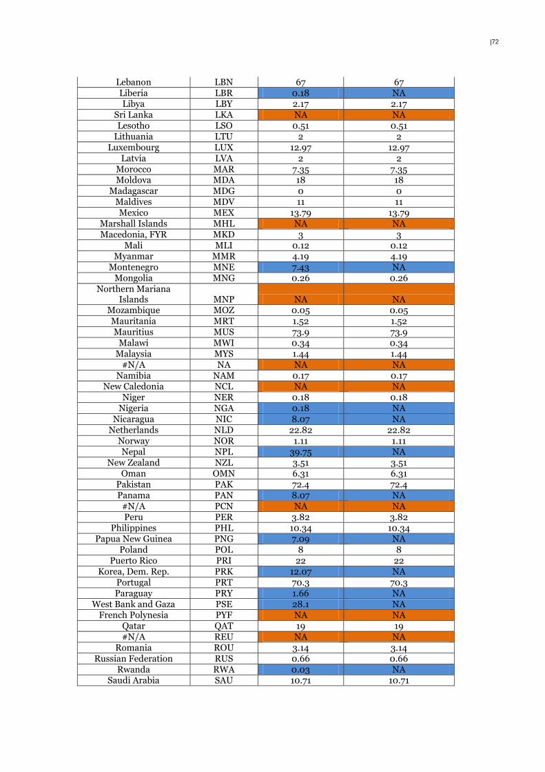
|72

Lebanon LBN 67 67 Liberia LBR 0.18 NA Libya LBY 2.17 2.17

Sri Lanka LKA NA NA Lesotho LSO 0.51 0.51

Lithuania LTU 2 2 Luxembourg LUX 12.97 12.97

Latvia LVA 2 2 Morocco MAR 7.35 7.35 Moldova MDA 18 18

Madagascar MDG 0 0 Maldives MDV 11 11 Mexico MEX 13.79 13.79

Marshall Islands MHL NA NA Macedonia, FYR MKD 3 3

Mali MLI 0.12 0.12 Myanmar MMR 4.19 4.19

Montenegro MNE 7.43 NA Mongolia MNG 0.26 0.26

Northern Mariana Islands MNP NA NA

Mozambique MOZ 0.05 0.05 Mauritania MRT 1.52 1.52 Mauritius MUS 73.9 73.9

Malawi MWI 0.34 0.34 Malaysia MYS 1.44 1.44

#N/A NA NA NA Namibia NAM 0.17 0.17

New Caledonia NCL NA NA Niger NER 0.18 0.18

Nigeria NGA 0.18 NA Nicaragua NIC 8.07 NA

Netherlands NLD 22.82 22.82 Norway NOR 1.11 1.11 Nepal NPL 39.75 NA

New Zealand NZL 3.51 3.51 Oman OMN 6.31 6.31

Pakistan PAK 72.4 72.4 Panama PAN 8.07 NA

#N/A PCN NA NA Peru PER 3.82 3.82

Philippines PHL 10.34 10.34 Papua New Guinea PNG 7.09 NA

Poland POL 8 8 Puerto Rico PRI 22 22

Korea, Dem. Rep. PRK 12.07 NA Portugal PRT 70.3 70.3 Paraguay PRY 1.66 NA

West Bank and Gaza PSE 28.1 NA French Polynesia PYF NA NA

Qatar QAT 19 19 #N/A REU NA NA

Romania ROU 3.14 3.14 Russian Federation RUS 0.66 0.66

Rwanda RWA 0.03 NA Saudi Arabia SAU 10.71 10.71

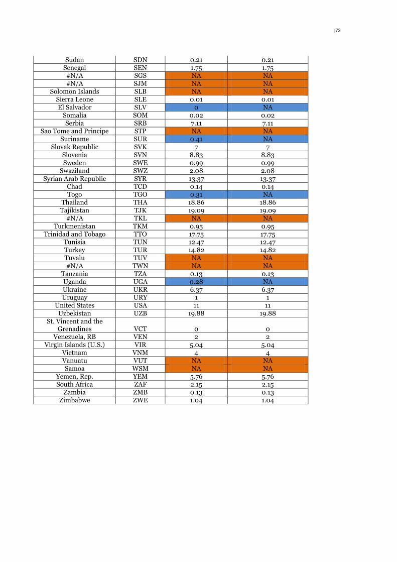
|73

Sudan SDN 0.21 0.21 Senegal SEN 1.75 1.75 #N/A SGS NA NA #N/A SJM NA NA

Solomon Islands SLB NA NA Sierra Leone SLE 0.01 0.01 El Salvador SLV 0 NA

Somalia SOM 0.02 0.02 Serbia SRB 7.11 7.11

Sao Tome and Principe STP NA NA Suriname SUR 0.41 NA

Slovak Republic SVK 7 7 Slovenia SVN 8.83 8.83 Sweden SWE 0.99 0.99

Swaziland SWZ 2.08 2.08 Syrian Arab Republic SYR 13.37 13.37

Chad TCD 0.14 0.14 Togo TGO 0.31 NA

Thailand THA 18.86 18.86 Tajikistan TJK 19.09 19.09

#N/A TKL NA NA Turkmenistan TKM 0.95 0.95

Trinidad and Tobago TTO 17.75 17.75 Tunisia TUN 12.47 12.47 Turkey TUR 14.82 14.82 Tuvalu TUV NA NA #N/A TWN NA NA

Tanzania TZA 0.13 0.13 Uganda UGA 0.28 NA Ukraine UKR 6.37 6.37 Uruguay URY 1 1

United States USA 11 11 Uzbekistan UZB 19.88 19.88

St. Vincent and the Grenadines VCT 0 0

Venezuela, RB VEN 2 2 Virgin Islands (U.S.) VIR 5.04 5.04

Vietnam VNM 4 4 Vanuatu VUT NA NA Samoa WSM NA NA

Yemen, Rep. YEM 5.76 5.76 South Africa ZAF 2.15 2.15

Zambia ZMB 0.13 0.13 Zimbabwe ZWE 1.04 1.04

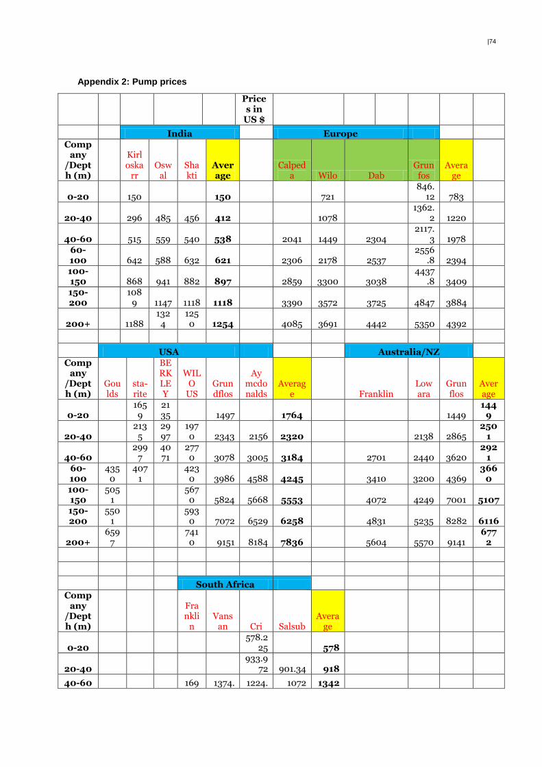
|74

Appendix 2: Pump prices

Prices in

US $ India Europe

Company

/Depth (m)

Kirloska

rr Osw

al Shakti

Average

Calpeda Wilo Dab

Grunfos

Average

0-20

150 150 721 846.

12 783

20-40

296 485 456 412 1078 1362.

2 1220

40-60

515 559 540 538 2041 1449 2304 2117.

3 1978 60-100

642 588 632 621 2306 2178 2537

2556.8 2394

100-150

868 941 882 897 2859 3300 3038

4437.8 3409

150-200

1089 1147 1118 1118 3390 3572 3725 4847 3884

200+

1188 1324

1250 1254 4085 3691 4442 5350 4392

USA Australia/NZ

Company

/Depth (m)

Goulds

sta-rite

BERKLEY

WILO

US Grundflos

Ay mcdonalds

Average Franklin

Lowara

Grunflos

Average

0-20 1659

2135 1497 1764 1449

1449

20-40 213

5 2997

1970 2343 2156 2320 2138 2865

2501

40-60 299

7 4071

2770 3078 3005 3184 2701 2440 3620

2921

60-100

4350

4071

4230 3986 4588 4245 3410 3200 4369

3660

100-150

5051

5670 5824 5668 5553 4072 4249 7001 5107

150-200

5501

5930 7072 6529 6258 4831 5235 8282 6116

200+ 659

7 7410 9151 8184 7836 5604 5570 9141

6772

South Africa

Company

/Depth (m)

Frankli

n Vans

an Cri Salsub Avera

ge

0-20

578.2

25 578

20-40

933.9

72 901.34 918

40-60

169 1374. 1224. 1072 1342

|75

8 27 9

60-100

2284

1570.18

1633.6 1420.2 1727

100-150

2771

1910.22 2341

150-200

3278

2480.14 2879

200+

359

9 2911.

43 3255

Appendix 3: Electricity prices: indexed to year 2005

Price

(IEA)

Climate

scope (2014

)a

Africa develop

ment bank group

(2005)b

Africa

report

(2009)c

Arab repo

rt (2015)d

Electricity

board (2015)e

Eeranet

(2013)f

Others

sourcesg

Price (US

cents/kwH)

Afghanistan 8.25 8.25

Albania 10.65

6 10.656

Algeria 2.676 2.676

Angola 3.377 3.377

Argentina 4.7 4.7

Armenia 5.099

9 5.09993

Australia 6.249 6.249

Austria 10.17

8 10.178 Azerbaija

n 5 5

Bahamas 24.48409

24.484092

Bahrain 3.04 3.04 Banglade

sh 8.332

Barbados 21.02 21.02

Belarus 3.8 3.8

Belgium 8.733 8.733

Belize 13.187

95 13.18794

7

Benin 10.7 10.7

Bermuda 25.17 25.17

Bhutan 2.12 2.12

Bolivia 4.8 4.8 Bosnia-

Herzegovina 9.648 9.648

Botswana 4 4

Brazil 7.71 7.71

Brunei 5.58 5.58

Bulgaria 7.016 7.016

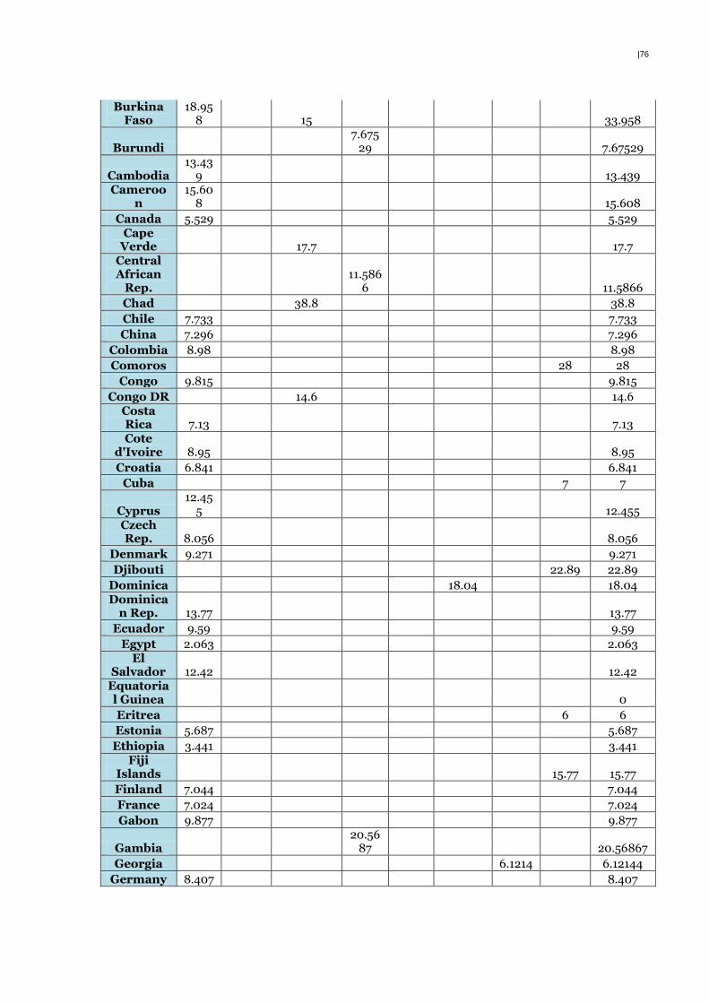
|76

Burkina Faso

18.958 15 33.958

Burundi 7.675

29 7.67529

Cambodia 13.43

9 13.439 Cameroo

n 15.60

8 15.608

Canada 5.529 5.529 Cape

Verde 17.7 17.7 Central African

Rep. 11.586

6 11.5866

Chad 38.8 38.8

Chile 7.733 7.733

China 7.296 7.296

Colombia 8.98 8.98

Comoros 28 28

Congo 9.815 9.815

Congo DR 14.6 14.6 Costa Rica 7.13 7.13 Cote

d'Ivoire 8.95 8.95

Croatia 6.841 6.841

Cuba 7 7

Cyprus 12.45

5 12.455 Czech Rep. 8.056 8.056

Denmark 9.271 9.271

Djibouti 22.89 22.89

Dominica 18.04 18.04 Dominica

n Rep. 13.77 13.77

Ecuador 9.59 9.59

Egypt 2.063 2.063 El

Salvador 12.42 12.42 Equatorial Guinea 0

Eritrea 6 6

Estonia 5.687 5.687

Ethiopia 3.441 3.441 Fiji

Islands 15.77 15.77

Finland 7.044 7.044

France 7.024 7.024

Gabon 9.877 9.877

Gambia 20.56

87 20.56867

Georgia 6.1214 6.12144

Germany 8.407 8.407

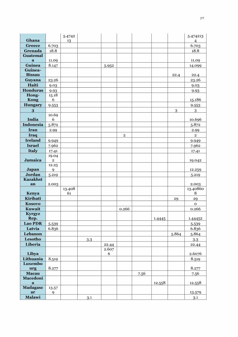
|77

Ghana 5.4742

13 5.474213

4

Greece 6.703 6.703

Grenada 18.8 18.8 Guatemal

a 11.09 11.09

Guinea 8.147 5.952 14.099 Guinea-Bissau 22.4 22.4

Guyana 23.26 23.26

Haiti 9.03 9.03

Honduras 9.93 9.93 Hong-Kong

15.186 15.186

Hungary 9.553 9.553

3 3 3

India 10.69

6 10.696

Indonesia 5.872 5.872

Iran 2.99 2.99

Iraq 2 2

Ireland 9.949 9.949

Israel 7.962 7.962

Italy 17.41 17.41

Jamaica 19.04

2 19.042

Japan 12.25

9 12.259

Jordan 5.219 5.219 Kazakhst

an 2.003 2.003

Kenya 13.408

61 13.40860

8

Kiribati 29 29

Kosovo 0

Kuwait 0.266 0.266 Kyrgyz

Rep. 1.4445 1.44452

Lao PDR 5.539 5.539

Latvia 6.836 6.836

Lebanon 5.864 5.864

Lesotho 3.3 3.3

Liberia 22.44 22.44

Libya 2.607

6 2.6076

Lithuania 8.519 8.519 Luxembo

urg 8.277 8.277

Macau 7.56 7.56 Macedoni

a 12.558 12.558 Madagasc

ar 13.57

9 13.579

Malawi 3.1 3.1

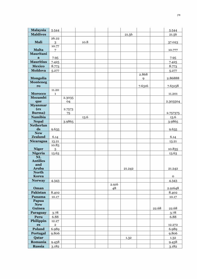
|78

Malaysia 5.544 5.544

Maldives 21.56 21.56

Mali 26.22

3 10.8 37.023

Malta 10.77

7 10.777 Mauritani

a 7.95 7.95

Mauritius 7.425 7.425

Mexico 8.773 8.773

Moldova 5.277 5.277

Mongolia 2.868

9 2.86888 Monteneg

ro 7.6316 7.63158

Morocco 11.20

1 11.201 Mozambi

que 2.3035

04 2.303504 Myanmar

(ex Burma)

2.757375 2.757375

Namibia 13.6 13.6

Nepal 3.9865 3.9865 Netherlan

ds 9.635 9.635 New

Zealand 6.14 6.14

Nicaragua 13.21 13.21

Niger 10.83

5 10.835

Nigeria 13.63 13.63 NL

Antilles and

Aruba 21.242 21.242 North Korea 0

Norway 4.343 4.343

Oman 2.916

48 2.91648

Pakistan 8.402 8.402

Panama 10.17 10.17 Papua New

Guinea 22.68 22.68

Paraguay 3.78 3.78

Peru 6.88 6.88 Philippin

es 12.27

2 12.272

Poland 6.989 6.989

Portugal 9.806 9.806

Qatar 1.32 1.32

Romania 9.458 9.458

Russia 3.182 3.182

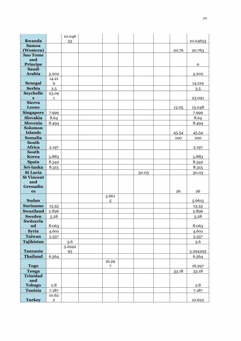
|79

Rwanda 10.046

53 10.04653 Samoa

(Western) 20.76 20.763 Sao Tome

and Principe 0

Saudi Arabia 3.202 3.202

Senegal 14.21

9 14.219

Serbia 3.5 3.5 Seychelle

s 23.09

1 23.091 Sierra Leone 13.05 13.048

Singapore 7.999 7.999

Slovakia 8.64 8.64

Slovenia 8.494 8.494 Solomon Islands 45.54 45.54

Somalia 100 100 South Africa 2.197 2.197 South Korea 5.883 5.883

Spain 8.342 8.342

Sri-lanka 8.315 8.315

St Lucia 30.03 30.03 St Vincent

and Grenadin

es 26 26

Sudan 5.661

5 5.6615

Suriname 13.33 13.33

Swaziland 2.896 2.896

Sweden 5.28 5.28 Switzerla

nd 8.063 8.063

Syria 4.601 4.601

Taiwan 5.557 5.557

Tajikistan 3.6 3.6

Tanzania 5.2942

93 5.294293

Thailand 6.564 6.564

Togo 16.29

7 16.297

Tonga 33.18 33.18 Trinidad

and Tobago 2.8 2.8

Tunisia 7.187 7.187

Turkey 10.62

2 10.622

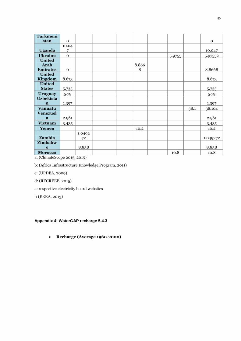
|80

Turkmenistan 0 0

Uganda 10.04

7 10.047

Ukraine 0 5.9755 5.97552 United Arab

Emirates 0 8.866

8 8.8668 United

Kingdom 8.673 8.673 United States 5.735 5.735

Uruguay 5.79 5.79 Uzbekista

n 1.397 1.397

Vanuatu 38.1 38.104 Venezuel

a 2.961 2.961

Vietnam 3.435 3.435

Yemen 10.2 10.2

Zambia 1.0492

72 1.049272 Zimbabw

e 8.838 8.838

Morocco 10.8 10.8 a: (ClimateScope 2015, 2015)

b: (Africa Infrastructure Knowledge Program, 2011)

c: (UPDEA, 2009)

d: (RECREEE, 2015)

e: respective electricity board websites

f: (ERRA, 2013)

Appendix 4: WaterGAP recharge 5.4.3

Recharge (Average 1960-2000)

|81

Depletion (Recharge – Abstractions)

Groundwater abstraction possible areas using WaterGAP recharge rates

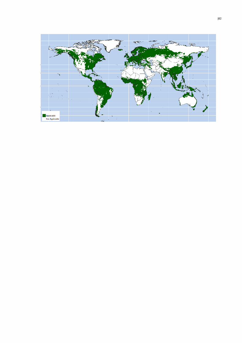
|82