evaluating the accuracy of motion tracking algorithms for
TRANSCRIPT
UPTEC IT 12 015
Examensarbete 30 hpSeptember 2012
Evaluating the accuracy of motion tracking algorithms for determining the position of finger tips
Malin Nilsson

Teknisk- naturvetenskaplig fakultet UTH-enheten Besöksadress: Ångströmlaboratoriet Lägerhyddsvägen 1 Hus 4, Plan 0 Postadress: Box 536 751 21 Uppsala Telefon: 018 – 471 30 03 Telefax: 018 – 471 30 00 Hemsida: http://www.teknat.uu.se/student
Abstract
Evaluating the accuracy of motion tracking algorithmsfor determining the position of finger tips
Malin Nilsson
Motion capture, or motion tracking, describes the process of recording movement ofobjects. Motion capture for biomechanical applications often involves sensors ormarkers that are placed on the skin of body segments. The position of these markersis measured as the subject moves. In this thesis, motion capture is used to recordmovements of the hand and fingers. Two methods for estimation of sensor positions,Method A and Method B, are investigated. These methods are based on kinematicmodels describing the studied system, where states are estimated with an ExtendedKalman Filter. In many applications it is important to estimate the position of thefinger tips accurately, but it is not always possible to place sensors on them.Therefore the methods are first modified to also estimate the positions of the fingertips based on the estimated positions of the markers. Then, the accuracy of themethods are evaluated in terms of a specific accuracy measure, for different values ofthe user parameters of the methods. The effect of the user parameters is investigatedand appropriate values for them, i.e values that give the best performance, are given.It is shown that Method B performs better than Method A and that it also is lesssensitive to the choice of user parameters, but Method A could be considered easierto use and easier to apply to general kinematic systems.
Tryckt av: ITCISSN: 1401-5749, UPTEC IT12 015Examinator: Arnold PearsÄmnesgranskare: Håkan LanshammarHandledare: Kjartan Halvorsen


Sammanfattning
Motion Capture, eller Motion Tracking, går ut på att mäta och spela in hurolika objekt rör sig. I biomekaniska tillämpningar av Motion Capture användsofta sensorer, eller markörer, som fästs på huden på olika kroppsdelar hos enförsöksperson. Man mäter sedan markörernas position, medan personen rörsig. I det här arbetet används Motion Capture för att spela in handens och�ngrarnas rörelser då �ngerspetsarna rör sig över en plan platta. Mätdatasom man får från sensorerna är brusiga och är därför inte alltid tillräckligt braför användning i vissa tillämpningar. För att minska bruset kan man användasig av metoder som brusreducerar med hjälp av kinematiska modeller avdet studerade systemet. Två sådana metoder undersökes i detta arbete. Imodellerna �nns variabler som beskriver olika vinklar och avstånd i systemet.Dessa variabler ändras med tiden och kan skattas med hjälp av ett så kallatExtended Kalman Filter (EKF). När alla vinklar och avstånd är kända kanför�nade versioner av sensormätningarna tas fram.
I många applikationer är det viktigt att bestämma �ngerspetsarnas po-sition noggrannt, men det är inte alltid möjligt att sätta sensorer på dem.Metoderna modi�eras därför först för att kunna bestämma �ngerspetsarnasposition utifrån de skattade markörpositionerna. I båda metoderna �nns ettantal parametrar som måste ställas in av användaren. Dessa parametrarpåverkar metodernas noggrannhet. Vilka värden som fungerar bäst beror påsystemet man studerar och det mätdata man samlat in. E�ekten av använ-darparametrarna på metodens noggrannhet undersöks och lämpliga värden,dvs värden som ger bäst prestation, på parametrarna ges. Det visar sig attMetod B presterar bättre än Metod A, och att den också är mindre känslig förvalet av användarparametrar, men Metod A kan ses som lättare att användaoch lättare att applicera på generella kinematiska system.

Contents
1 Introduction 5
2 Method 72.1 Modelling . . . . . . . . . . . . . . . . . . . . . . . . . . . . . 7
2.1.1 Method A . . . . . . . . . . . . . . . . . . . . . . . . . 72.1.2 Method B . . . . . . . . . . . . . . . . . . . . . . . . . 12
2.2 Experiment . . . . . . . . . . . . . . . . . . . . . . . . . . . . 132.2.1 Finding the �nger tip . . . . . . . . . . . . . . . . . . . 142.2.2 User Parameters . . . . . . . . . . . . . . . . . . . . . 16
3 Results 193.1 Method A . . . . . . . . . . . . . . . . . . . . . . . . . . . . . 193.2 Method B . . . . . . . . . . . . . . . . . . . . . . . . . . . . . 253.3 Performance . . . . . . . . . . . . . . . . . . . . . . . . . . . . 25
4 Conclusions and Discussion 314.1 Results . . . . . . . . . . . . . . . . . . . . . . . . . . . . . . . 314.2 Initial Guesses . . . . . . . . . . . . . . . . . . . . . . . . . . . 324.3 Position of the Finger Tip . . . . . . . . . . . . . . . . . . . . 334.4 The Accuracy Measure . . . . . . . . . . . . . . . . . . . . . . 334.5 Future Studies . . . . . . . . . . . . . . . . . . . . . . . . . . . 34
3


Chapter 1
Introduction
Motion capture, or motion tracking, describes the process of recording move-
ment of objects. It is used in military, entertainment, sports, medical appli-
cations and more [1]. Motion capture for biomechanical applications often
involves sensors or markers that are placed on the skin of body segments.
The position of these markers is measured as the subject moves. The col-
lected data can then be used to reconstruct the motion of the body part.
The system described in [2] is designed for interacting with 3D, virtual and
dynamic objects rendered by a holographic display. The system includes a
haptic glove which makes you experience that you are grabbing an actual
physical object. One application for this is in jaw surgery, where the surgeon
could use this technique to practice di�cult operations without running the
risk of injuring a patient. Motion capture is an important element of this. If
the haptic glove is to work as expected, the positions of the tips of the �ngers
have to be known. The measured data from the markers is noisy, which could
be a problem, therefore it may be important to use motion capture models
to �lter the data to remove the noise.
The purpose of this project is to modify two existing motion capture
model implementations, and then to investigate and compare the accuracy
of the two methods for estimating the position of the tips of the �ngers from
motion capture data. The implementations must �rst be modi�ed to only
describe the hand and �nger movements, and then equations must be added
5
to calculate the coordinates of the �nger tips. The tracking algorithms and
their ability to reconstruct the �nger positions from measured data must
then be evaluated. Speci�cally, the precision of the algorithms when esti-
mating the �nger tip positions as they move over a known surface must be
established. Therefore an appropriate accuracy measure must be chosen and
applied. More speci�cally, the goals are:
• To �nd out which is the better method.
• To establish whether any of the methods improve the results compared
to using measured data directly.
• To determine how important the choice of the user parameters are in
the two methods.
The reason for doing this is to simplify future studies of virtual object in-
teraction by providing a reliable estimation method. The �rst of the two
implementations that will be modi�ed is a toolbox by Todorov (2007) [3]
that contains a framework for constructing kinematic models of general seg-
ments and joint structures. The second was derived by Halvorsen et al.
(2008) [4]. It estimates the movement of the forearm, the palm and all �ve
�ngers. These two methods will be adapted to model the forearm, the hand,
the index �nger and the middle �nger.
6
Chapter 2
Method
2.1 Modelling
In this study we choose to model only the forearm, the hand and two �ngers.
The forearm and hand can be described by a number of segments connected
by joints. The hand is one segment, the forearm is one segment and each �n-
ger consist of three segments. One sensor was placed on each �nger segment;
the distal phalange, the intermediate phalange and the proximal phalange.
Two were placed on the palm of the hand, and three sensors were placed
on the forearm. All sensors were placed on the skin except for the one on
the distant phalange which was placed on the nail. Two approaches were
used to model this and to estimate the model states, one by Todorov and
one by Halvorsen et al. The method derived by Todorov will be referred to
as Method A and the one based on the model by Halvorsen et al. will be
referred to as Method B.
2.1.1 Method A
Todorov has developed a toolbox for movement estimation and self-calibration
from motion capture data, and we will use this toolbox to create a model
for the forearm and hand and estimate its states. Using the toolbox involves
three steps.
1. Constructing a kinematic model specifying how the sensor measure-
7
ments depend on the state vector. The model also requires speci�cation
of the process noise covariance matrix R.
2. Collecting motion-capture data compatible with the model created in
step 1.
3. Applying the estimation algorithm. Initial values for the state vector
and the state covariance matrix are required.
In each time step the model decides a maximum aposteriori estimation of the
state vector by using an iterative algorithm. If only one iteration is carried
out the algorithm is an extended Kalman �lter.
Before this toolbox could be used, the system, i.e. all the joints and how
they are connected, had to be described in detail. The kinematic model could
then be described as an Nx5 matrix where N is the number of segments. The
integers in the matrix decide the properties of the model. To give more clar-
ity this model has, with the help of the matrix, been drawn as a tree shown in
�gure 2.1. In this tree the segments can correspond to limb segments, dummy
segments or sensors, which are all connected by joints. Rectangles represent
segments/frames and circles represent joints/transformations. Shaded cir-
cles correspond to constant transformations while empty circles corresponds
to time-varying transformations. Rectangles with heavy outlines represent
frames whose position are being measured by sensors. Two segments can
only be connected with a single joint, so if there is both a translation and a
rotation of the same joint a dummy segment needs to be placed between the
two joints.
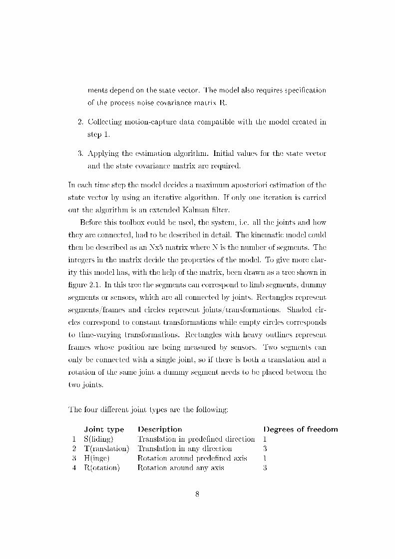
The four di�erent joint types are the following:
Joint type Description Degrees of freedom1 S(liding) Translation in prede�ned direction 12 T(ranslation) Translation in any direction 33 H(inge) Rotation around prede�ned axis 14 R(otation) Rotation around any axis 3
8
1. Sliding joints have one parameter specifying the sliding distance.
2. Translation joints have three parameters, which specify the translation
vector.
3. Hinge joints have one parameter, specifying the rotation angle.
4. Rotation joints have three parameters, specifying an angle-axis vector.
The length of this vector is the rotation angle, and the direction of the
vector is the rotation axis.
The states of this model are the free parameters of each joint. Since joints
can be set as �xed, constant but unknown parameters, such as limb lengths,
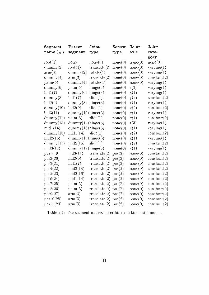
can be estimated using this model. The kinematic tree can be represented
as a table, which contains all information about the segments and their con-
necting joints. Fig. 2.1 is represented in tabular form in table 2.1. The state
equations are given by
xj(k + 1) = xj(k) + uj(k) (2.1)
where xj is the j:th state variable and uj(k) is white noise with variance σ2j ,
the process noise. For states representing constant parameters, σ2j is set to
0. This means that the state estimator will assume that these states do not
change in time. The output from the model is given by
y(k) = f(x) + µ(k) (2.2)
where y contains the coordinates for all sensors, f is the nonlinear function
describing how the markers depend on the states and µ(k) is white measure-
ment noise with
E[µ(k)µT (k)] = Rµ(k). (2.3)
9
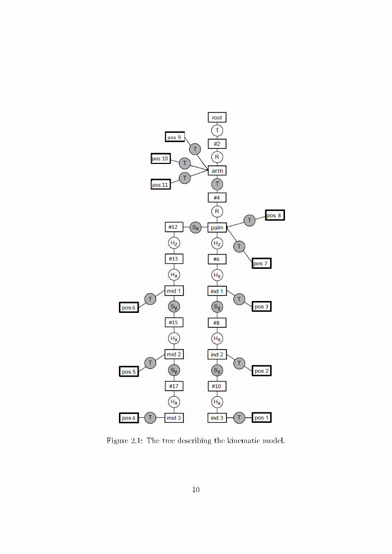
Figure 2.1: The tree describing the kinematic model.
10
Segmentname (#)
Parentsegment
Jointtype
Sensortype
Jointaxis
Jointcate-gory
root(1) none none(0) none(0) none(0) none(0)dummy(2) root(1) translate(2) none(0) none(0) varying(1)arm(3) dummy(2) rotate(4) none(0) none(0) varying(1)dummy(4) arm(3) translate(2) none(0) none(0) constant(2)palm(5) dummy(4) rotate(4) none(0) none(0) varying(1)dummy(6) palm(5) hinge(3) none(0) z(3) varying(1)ind1(7) dummy(6) hinge(3) none(0) x(1) varying(1)dummy(8) ind1(7) slide(1) none(0) y(2) constant(2)ind2(9) dummy(8) hinge(3) none(0) x(1) varying(1)dummy(10) ind2(9) slide(1) none(0) y(2) constant(2)ind3(11) dummy(10)hinge(3) none(0) x(1) varying(1)dummy(12) palm(5) slide(1) none(0) x(1) constant(2)dummy(13) dummy(12)hinge(3) none(0) z(3) varying(1)mid1(14) dummy(13)hinge(3) none(0) x(1) varying(1)dummy(15) mid1(14) slide(1) none(0) y(2) constant(2)mid2(16) dummy(15)hinge(3) none(0) x(1) varying(1)dummy(17) mid2(16) slide(1) none(0) y(2) constant(2)mid3(18) dummy(17)hinge(3) none(0) x(1) varying(1)pos1(19) ind3(11) translate(2) pos(2) none(0) constant(2)pos2(20) ind2(9) translate(2) pos(2) none(0) constant(2)pos3(21) ind1(7) translate(2) pos(2) none(0) constant(2)pos4(22) mid3(18) translate(2) pos(2) none(0) constant(2)pos5(23) mid2(16) translate(2) pos(2) none(0) constant(2)pos6(24) mid1(14) translate(2) pos(2) none(0) constant(2)pos7(25) palm(5) translate(2) pos(2) none(0) constant(2)pos8(26) palm(5) translate(2) pos(2) none(0) constant(2)pos9(27) arm(3) translate(2) pos(2) none(0) constant(2)pos10(28) arm(3) translate(2) pos(2) none(0) constant(2)pos11(29) arm(3) translate(2) pos(2) none(0) constant(2)
Table 2.1: The segment matrix describing the kinematic model.
11

2.1.2 Method B
The model derived by Halvorsen et al. is presented in [4]. It is a dynamic
model on state space form, where the states are the angles and their angular
velocities and the output signal is the markers' position coordinates. The
angular velocities are modelled as random walks and the angles as the integral
of the velocities. The output signal is written as a function of the states by
means of rotation matrices. This function is nonlinear so a standard Kalman
�lter can not be used to estimate the states. Instead, an extended Kalman
�lter (EKF) is used.
The model equations can be derived as follows: Let φ(t) be the joint
angles in the model. The assumption in the model is that each angular
acceleration is white noise, i.e
φ(k) = w(k) (2.4)
where w(k) is white noise with the covariance matrix
E[w(k)wT (k + τ)] = Rwδ(τ) (2.5)
where δ(τ) is Dirac's δ function and Rw is a diagonal matrix. Let x(k) be the
state vector in the model. The �rst half of the vector consists of the angles
φ(k) and the second half consists of their angular velocities φ(k). It is shown
in [4] that the state equations for x(k) then becomes
x(k + 1) = Fx(k) + v(k) =
[I hI0 I
]x(k) + v(k) (2.6)
where I is the identity matrix and h is the sampling period. The covariance
matrix of the process noise v(k) has the form
E[v(k)vT (k)] =
[(1/3)h3Rw(k) (1/2)h2Rw(k)(1/2)h2Rw(k) hRw(k)
]. (2.7)
The output from the model is given by
y(k) = vect([G(1)(k)p
(1)0 . . .G(L)(k)p
(L)0
]) + e(k) (2.8)
12

where p(i)0 contains the coordinates for all markers on segment i when the
system is in its reference position, and the matrices G(i)(k) are functions
of φ(k) describing the rotation of each segment. p(i)0 (k) are matrices where
each column contains the coordinates for one marker, the vect-function stacks
these columns in one single vector. e(k) is white noise with
E[e(k)eT (k)] = Re(k). (2.9)
The behavior of the EKF will depend on how Rw in (2.5) and Re in (2.9)
are chosen.
The model in [4] includes �ve �ngers, the hand and the arm. Since we only
look at the index �nger and the middle �nger in this work, it is unneccessary
to perform time-consuming calculations for the other �ngers. Three �ngers
were therefore removed from the model, the thumb, the ring �nger and the
little �nger. The model then becomes simpler with fewer states and outputs
and the calculations will be performed faster.
2.2 Experiment
To determine the accuracy of the methods an experiment was conducted.
Markers were placed on each segment of the hand of a test subject and on
a horizontal plate. More speci�cally, re�ective markers, half-spheres of 2mm
diameter, were attached using double-sided tape on the dorsal side of each
joint of each �nger. Three markers were also attached to the dorsal side of
the palm, one on the ulnar styloid, one on the radial styloid, and one directly
proximal to this along the radius. A photoelectric motion capture system
(Oqus, Qualisys AB, Gothenburg) consisting of 8 cameras was used to track
the 3D position of the markers in a measurement volume approximately 1m3.
The frame rate of the system was 250 fps.
The test subject was asked to draw an eight with the index �nger and the
middle �nger on the plate. When the �nger is on the plate the z-coordinate
of the �nger tip is the same as that of the plate. All deviation from this value
in the simulated z-coordinate must therefore be due to model uncertainty.
13
The mean square error between the z-coordinate of the �nger tip and that of
the plate is thus one possible measure of model accuracy. One way to check
if the model succeeded with the noise reduction is to compare the variance
of the modelled position of the marker with the variance of the measured
position of the marker, during the time in which the �nger is on the plate.
To calculate the variance from measured data, we use the sample variance
formula
v =1
N − 1
N∑i=1
(yi − y)2 (2.10)
where yi, i = 1, . . . , N are the measured data points, n is the number of
samples and y is the sample mean
y =1
N
N∑i=1
y(i). (2.11)
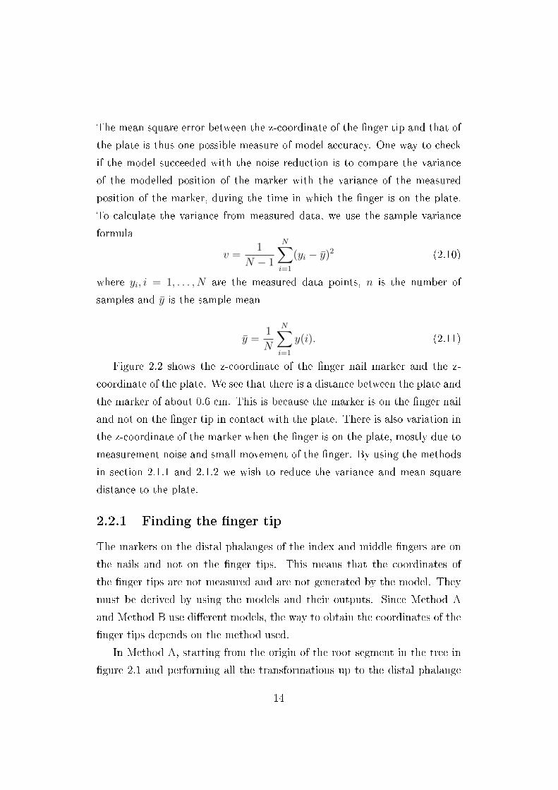
Figure 2.2 shows the z-coordinate of the �nger nail marker and the z-
coordinate of the plate. We see that there is a distance between the plate and
the marker of about 0.6 cm. This is because the marker is on the �nger nail
and not on the �nger tip in contact with the plate. There is also variation in
the z-coordinate of the marker when the �nger is on the plate, mostly due to
measurement noise and small movement of the �nger. By using the methods
in section 2.1.1 and 2.1.2 we wish to reduce the variance and mean square
distance to the plate.
2.2.1 Finding the �nger tip
The markers on the distal phalanges of the index and middle �ngers are on
the nails and not on the �nger tips. This means that the coordinates of
the �nger tips are not measured and are not generated by the model. They
must be derived by using the models and their outputs. Since Method A
and Method B use di�erent models, the way to obtain the coordinates of the
�nger tips depends on the method used.
In Method A, starting from the origin of the root segment in the tree in
�gure 2.1 and performing all the transformations up to the distal phalange
14
0 5 10 15 20 25 30 35 40 45
−0.02
0
0.02
0.04
0.06
0.08
Time (s)
z−co
ordi
nate
(m
)
Finger tip markerSurface
Figure 2.2: The z-coordinate of the measured position of the marker and thez-coordinate of the plate.
segment gives the coordinates of the segment origin. This is a point in
the center of the �nger where the distal phalange starts. The �nger tip
coordinates can be acquired by moving an appropriate distance along the
segment's main axis. In order to do this, the orientation of the segment
must be known at all times. The orientation is obtained by combining the
rotation transformations between the root segment and the distal phalange
segment in the tree in �gure 2.1. These calculations involve lots of matrix
multiplications and are not included here.
One of the outputs of the model in Method B gives the coordinates for
the centre of mass of the distal phalange. To obtain the coordinates of the
tip of the �nger in this case, the same approach as in Method A can be used,
but adding a distance to the centre of mass instead of the origin of the last
�nger segment.
Matematically, the way of �nding the �nger tip can be written as follows.
15

Assume x0 are the coordinates of a point in the middle of the �nger. Assume
that the tip of the �nger is at a distance d along the axis given by the vector
v. The coordinates xt for the �nger tip is then obtained by
xt = x0 + dv. (2.12)
2.2.2 User Parameters
In both methods there are di�erent user parameters which have to be set in
advance.
In Method A the process noise σ2j in (2.1) and the measurement noise Rµ
in (2.3) have to be speci�ed. Large process noise for a state variable means
that you think that the variation is large in that state, which means you have
less trust in the model. The toolbox in Method A lets you specify one single
parameter, which is then used to calculate σ2j of each state in the model.
The unit of each element in the process noise vector varies depending on its
corresponding state. So it can be either m/s or rad/s, since states can be
rotations and translations. The user parameter is unitless.
Since lengths of segments are estimated in this method it could be im-
portant to have accurate initial guesses for them. The initial values can be
calculated in di�erent ways. Since each segment has a marker and the mark-
ers are placed approximately in the middle of each segment, the lengths of
the segments can be estimated by using the measured mean distance between
the markers over time, during an experiment.
In Method B the lengths of the segments are not needed to specify the
model. The parameters Rw and Re in (2.5) and (2.9) must be chosen. Rw
is calculated in the program code by using a tuning parameter ω. This
parameter is used to decide the bandwidth of a �lter that �lters the process
noise in the model. The larger the parameter the higher the bandwidth in
the �lter which results in larger noise. The parameter itself has no unit.
Rµ and Re are guesses of how large the measurement noise in the sensors
are, and was already set in the program code of each method.
16

It is not possible to know in advance which the best parameters are.
Di�erent parameters must be tested and the results must be evaluated to
�nd out which set of parameters gives the best results.
17


Chapter 3
Results
Both methods were run with di�erent values of the user parameters and the
mean square error between both the index �nger tip and the middle �nger
tip and the plate were calculated for each case. The positions of the �nger
tips were calculated using the model output and the method in section 2.2.1.
The results are shown below. The variance of the modelled z-coordinate of
the �nger nail marker was also calculated for each case.
3.1 Method A
The method was applied to the measured data using three di�erent values of
the user parameter deciding the process noises and two sets of initial values
for the segment lengths. The user parameter was 5, 50 and 200. At �rst,
all the initial values for the segment lengths and the distance between the
knuckles were set to zero and were then changed to the values given by table
3.1. These values were calculated in the way described in section 2.2.2. The
initial values of all other states were set to zero.
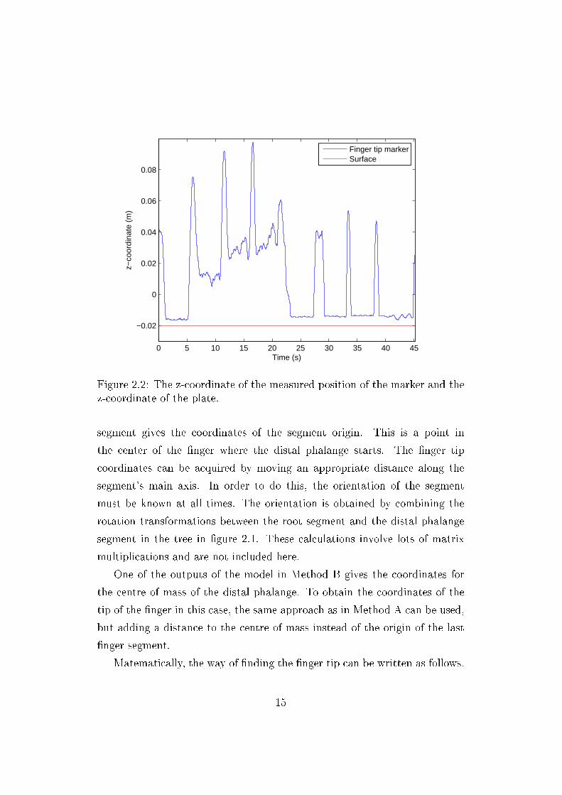
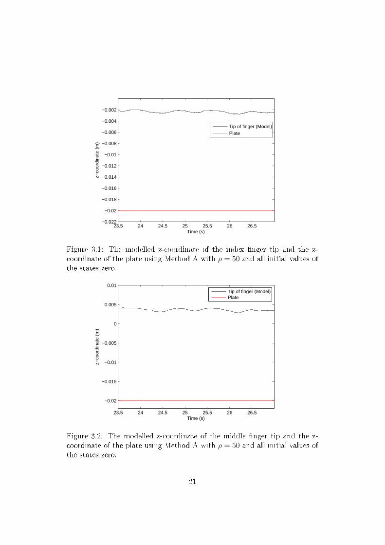
Figures 3.1 and 3.2 show the modelled z-coordinate of the index �nger tip
and and the middle �nger tip respectively and the z-coordinate of the plate
when the process noise parameter ρ was 50 and the initial values were zero,
during the time in which the �nger was on the plate. It can be seen that
the position of the �nger tip is not well estimated by the method in this case
since there seems to be a distance of about 1.8 cm between the estimated
19

State description State num-ber
Initial value(cm)
Length of intermediate phalangeof the index �nger
15 3.24
Length of proximal phalange ofthe index �nger
17 4.94
Length of intermediate phalangeof the middle �nger
22 3.77
Length of proximal phalange ofthe middle �nger
24 5.63
Distance between knuckles 19 3.10
Table 3.1: Initial values for the segment lengths and the distance betweenthe knuckles, and their corresponding state number in the model. Calculatedin the way described in 2.2.2
index �nger tip position and the real one, and 1.5 cm between the estimated
middle �nger tip position and the real one.
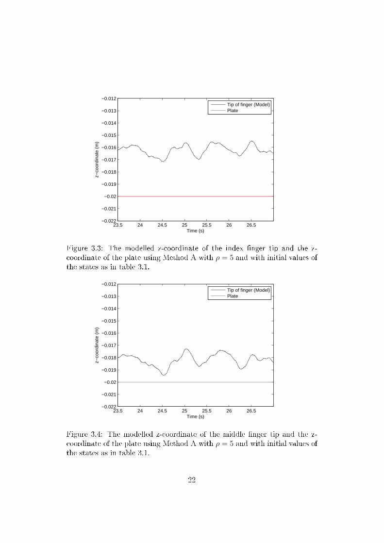
Figures 3.3 and 3.4 show the modelled z-coordinate of the index �nger tip
and the middle �nger tip respectively and the z-coordinate of the plate when
the process noise parameter ρ was 5 and the initial values were as in table
3.1, during the time in which the �nger was on the plate. We see that this
estimation is also poor, but better than in the case without initial guesses.
The distance between the estimated index �nger tip position and the real
one is around 0.4 cm and the one between the estimated middle �nger tip
position and the real one is around 0.2 cm.
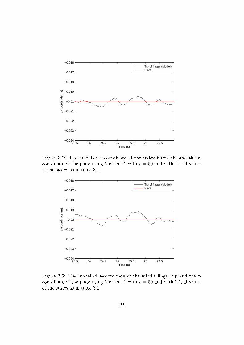
Figures 3.5 and 3.6 show the modelled z-coordinate of the index �nger
tip and the middle �nger tip respectively and the z-coordinate of the plate
when the process noise parameter ρ was 50 and the initial values were as in
table 3.1, during the time in which the �nger was on the plate. In this case
the estimation is better since the z-coordinate of the �nger tip seems to be
close to that of the plate. We can also see that the variance of the modelled
�nger tip position is lower here.
Figures 3.7 and 3.8 show the modelled z-coordinate of the index �nger tip
and the middle �nger tip respectively and the z-coordinate of the plate when
20
23.5 24 24.5 25 25.5 26 26.5−0.022
−0.02
−0.018
−0.016
−0.014
−0.012
−0.01
−0.008
−0.006
−0.004
−0.002
Time (s)
z−co
ordi
nate
(m
)
Tip of finger (Model)Plate
Figure 3.1: The modelled z-coordinate of the index �nger tip and the z-coordinate of the plate using Method A with ρ = 50 and all initial values ofthe states zero.
23.5 24 24.5 25 25.5 26 26.5
−0.02
−0.015
−0.01
−0.005
0
0.005
0.01
Time (s)
z−co
ordi
nate
(m
)
Tip of finger (Model)Plate
Figure 3.2: The modelled z-coordinate of the middle �nger tip and the z-coordinate of the plate using Method A with ρ = 50 and all initial values ofthe states zero.
21
23.5 24 24.5 25 25.5 26 26.5−0.022
−0.021
−0.02
−0.019
−0.018
−0.017
−0.016
−0.015
−0.014
−0.013
−0.012
Time (s)
z−co
ordi
nate
(m
)
Tip of finger (Model)Plate
Figure 3.3: The modelled z-coordinate of the index �nger tip and the z-coordinate of the plate using Method A with ρ = 5 and with initial values ofthe states as in table 3.1.
23.5 24 24.5 25 25.5 26 26.5−0.022
−0.021
−0.02
−0.019
−0.018
−0.017
−0.016
−0.015
−0.014
−0.013
−0.012
Time (s)
z−co
ordi
nate
(m
)
Tip of finger (Model)Plate
Figure 3.4: The modelled z-coordinate of the middle �nger tip and the z-coordinate of the plate using Method A with ρ = 5 and with initial values ofthe states as in table 3.1.
22
23.5 24 24.5 25 25.5 26 26.5−0.024
−0.023
−0.022
−0.021
−0.02
−0.019
−0.018
−0.017
−0.016
Time (s)
z−co
ordi
nate
(m
)
Tip of finger (Model)Plate
Figure 3.5: The modelled z-coordinate of the index �nger tip and the z-coordinate of the plate using Method A with ρ = 50 and with initial valuesof the states as in table 3.1.
23.5 24 24.5 25 25.5 26 26.5−0.024
−0.023
−0.022
−0.021
−0.02
−0.019
−0.018
−0.017
−0.016
Time (s)
z−co
ordi
nate
(m
)
Tip of finger (Model)Plate
Figure 3.6: The modelled z-coordinate of the middle �nger tip and the z-coordinate of the plate using Method A with ρ = 50 and with initial valuesof the states as in table 3.1.
23

23.5 24 24.5 25 25.5 26 26.5−0.024
−0.023
−0.022
−0.021
−0.02
−0.019
−0.018
−0.017
−0.016
Time (s)
z−co
ordi
nate
(m
)
Tip of finger (Model)Plate
Figure 3.7: The modelled z-coordinate of the index �nger tip and the z-coordinate of the plate using Method A with ρ = 200 and with initial valuesof the states as in table 3.1.
23.5 24 24.5 25 25.5 26 26.5−0.024
−0.023
−0.022
−0.021
−0.02
−0.019
−0.018
−0.017
−0.016
Time (s)
z−co
ordi
nate
(m
)
Tip of finger (Model)Plate
Figure 3.8: The modelled z-coordinate of the middle �nger tip and the z-coordinate of the plate using Method A with ρ = 200 and with initial valuesof the states as in table 3.1.
24

the process noise parameter ρ was 200 and the initial values were as in table
3.1, during the time in which the �nger was on the plate. This estimation
is worse than the one shown in �gure 3.5 but better than the estimation in
3.3. For each choice of the process noise parameter ρ and initial values the
mean square error was calculated between the modelled z-coordinate of the
�nger tip and the z-coordinate of the plate. The variance of the modelled
z-coordinate of the �nger tip marker was also calculated.
3.2 Method B
The method was applied to the measured data using three di�erent �lter
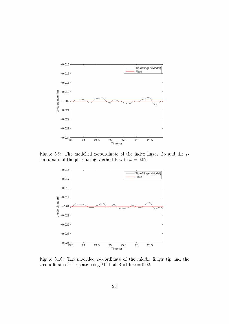
parameters, ω = 0.02, ω = 1 and ω = 100. Figures 3.9 and 3.10 show
the modelled z-coordinate of the index �nger tip and the middle �nger tip
respectively and the z-coordinate of the plate when the �lter parameter ω
was 0.02, during the time in which the �nger was on the plate. Figures
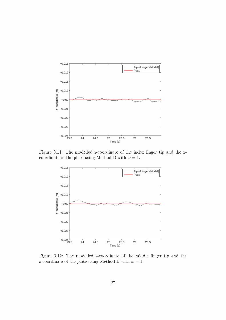
3.11 and 3.12 show the modelled z-coordinate of the index �nger tip and
the middle �nger tip respectively and the z-coordinate of the plate when the
�lter parameter ω was 1, during the time in which the �nger was on the plate.
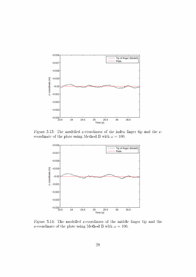
Figures 3.13 and 3.14 show the modelled z-coordinate of the index �nger tip
and the middle �nger tip respectively and the z-coordinate of the plate when
the �lter parameter ω was 100, during the time in which the �nger was on
the plate. In all three cases the estimated �nger tip z-coordinates are close to
that of the plate, but when the �lter parameter ω = 1 the variance is smaller
than in the other two cases. The variance is the largest when ω = 0.02.
3.3 Performance
To compare the accuracy of the two methods the mean square error between
the model z-coordinate of the �nger tips and that of the plate in each case
for each method was calculated. To check whether the methods succeeded in
reducing the measurement noise, the variance of the modelled z-coordinate
of the �nger nail marker on each �nger was calculated and compared to that
25
23.5 24 24.5 25 25.5 26 26.5−0.024
−0.023
−0.022
−0.021
−0.02
−0.019
−0.018
−0.017
−0.016
Time (s)
z−co
ordi
nate
(m
)
Tip of finger (Model)Plate
Figure 3.9: The modelled z-coordinate of the index �nger tip and the z-coordinate of the plate using Method B with ω = 0.02.
23.5 24 24.5 25 25.5 26 26.5−0.024
−0.023
−0.022
−0.021
−0.02
−0.019
−0.018
−0.017
−0.016
Time (s)
z−co
ordi
nate
(m
)
Tip of finger (Model)Plate
Figure 3.10: The modelled z-coordinate of the middle �nger tip and thez-coordinate of the plate using Method B with ω = 0.02.
26
23.5 24 24.5 25 25.5 26 26.5−0.024
−0.023
−0.022
−0.021
−0.02
−0.019
−0.018
−0.017
−0.016
Time (s)
z−co
ordi
nate
(m
)
Tip of finger (Model)Plate
Figure 3.11: The modelled z-coordinate of the index �nger tip and the z-coordinate of the plate using Method B with ω = 1.
23.5 24 24.5 25 25.5 26 26.5−0.024
−0.023
−0.022
−0.021
−0.02
−0.019
−0.018
−0.017
−0.016
Time (s)
z−co
ordi
nate
(m
)
Tip of finger (Model)Plate
Figure 3.12: The modelled z-coordinate of the middle �nger tip and thez-coordinate of the plate using Method B with ω = 1.
27
23.5 24 24.5 25 25.5 26 26.5−0.024
−0.023
−0.022
−0.021
−0.02
−0.019
−0.018
−0.017
−0.016
Time (s)
z−co
ordi
nate
(m
)
Tip of finger (Model)Plate
Figure 3.13: The modelled z-coordinate of the index �nger tip and the z-coordinate of the plate using Method B with ω = 100.
23.5 24 24.5 25 25.5 26 26.5−0.024
−0.023
−0.022
−0.021
−0.02
−0.019
−0.018
−0.017
−0.016
Time (s)
z−co
ordi
nate
(m
)
Tip of finger (Model)Plate
Figure 3.14: The modelled z-coordinate of the middle �nger tip and thez-coordinate of the plate using Method B with ω = 100.
28

of the measured z-coordinate. These values are shown in tables 3.2 and 3.3.
The variance of the measured z-coordinate of the index �nger was 3.74 · 10−8
and of the middle �nger was 5.48 · 10−8. These variances were calculated
using the sample variance formula in (2.10).
In Method A the mean square error was the smallest when using better
initial values for the states and with ρ = 50. Changing the initial states in-
creases the mean square error signi�cantly, and so does changing the process
noise parameter ρ. The variances of the estimated marker positions obtained
from the model, were smaller than those obtained from the measured data,
in all cases except for when the process noise parameter ρ was 5.
In Method B the mean square error was the smallest when ω was 1.
Changing the �lter parameter increased the mean square error, but not as
much as when changing the process noise parameter ρ in Method A. In this
case the variances of the estimated marker positions obtained from the model
were smaller than those obtained from the measured data, in all cases except
for when ω was 0.02 in the index �nger case.
29
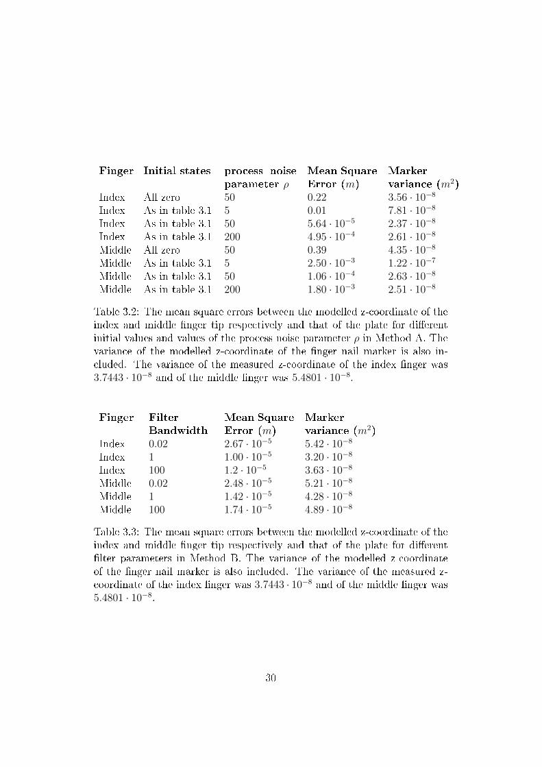
Finger Initial states process noiseparameter ρ
Mean SquareError (m)
Markervariance (m2)
Index All zero 50 0.22 3.56 · 10−8
Index As in table 3.1 5 0.01 7.81 · 10−8
Index As in table 3.1 50 5.64 · 10−5 2.37 · 10−8
Index As in table 3.1 200 4.95 · 10−4 2.61 · 10−8
Middle All zero 50 0.39 4.35 · 10−8
Middle As in table 3.1 5 2.50 · 10−3 1.22 · 10−7
Middle As in table 3.1 50 1.06 · 10−4 2.63 · 10−8
Middle As in table 3.1 200 1.80 · 10−3 2.51 · 10−8
Table 3.2: The mean square errors between the modelled z-coordinate of theindex and middle �nger tip respectively and that of the plate for di�erentinitial values and values of the process noise parameter ρ in Method A. Thevariance of the modelled z-coordinate of the �nger nail marker is also in-cluded. The variance of the measured z-coordinate of the index �nger was3.7443 · 10−8 and of the middle �nger was 5.4801 · 10−8.
Finger FilterBandwidth
Mean SquareError (m)
Markervariance (m2)
Index 0.02 2.67 · 10−5 5.42 · 10−8
Index 1 1.00 · 10−5 3.20 · 10−8
Index 100 1.2 · 10−5 3.63 · 10−8
Middle 0.02 2.48 · 10−5 5.21 · 10−8
Middle 1 1.42 · 10−5 4.28 · 10−8
Middle 100 1.74 · 10−5 4.89 · 10−8
Table 3.3: The mean square errors between the modelled z-coordinate of theindex and middle �nger tip respectively and that of the plate for di�erent�lter parameters in Method B. The variance of the modelled z-coordinateof the �nger nail marker is also included. The variance of the measured z-coordinate of the index �nger was 3.7443 · 10−8 and of the middle �nger was5.4801 · 10−8.
30
Chapter 4
Conclusions and Discussion
4.1 Results
In table 3.2 and 3.3 we see that, based on the mean square error, Method B
performs signi�cantly better than Method A. All values of the mean square
error in Method B are lower than the corresponding values in Method A.
However, the mean square error in Method A, when the process noise pa-
rameter ρ = 50, is of the same order of magnitude as the mean square error
in Method B, which means that as long as the choice of process noise pa-
rameter in Method A is good, it will perform almost as good as Method B.
If we instead look at the variance of the modelled z-coordinate of the marker
on the �nger nail, it is about the same size for both methods. This indicates
that both methods are equally good at reducing noise, but since we just saw
that Method B performs better in terms of mean square error, the variance
is not a good enough measure for determining which method works the best.
Both methods succeed in lowering the variance of the position of the marker
(for a good choice of process noise parameter/�lter parameter) in comparison
to the measured data, which indicates that the methods eliminates some of
the noise.
The results of Method A depend a lot on both the choice of the process
noise parameter and the initial guesses for the states, as can be seen in �gures
3.1-3.8 and table 3.2. Choosing the wrong process noise parameter gives more
31

variance in the modelled z-coordinate of the �nger tip, which means that the
noise reduction is not as good. We can also see in �gures 3.3, 3.4 and �gure
3.7, 3.8 that the estimation of the position of the tip of the �nger is incorrect
if the wrong process noise parameter is chosen. When changing the process
noise parameter from 50 to 5 the mean square error gets approximately 20
times larger, and when changing it from 50 to 200 it gets about 10 times
larger. This is a problem since the exact process noise in the system is rarely
known, and it is not always possible to guess an accurate value for it. In our
experiment we knew that the �nger tip was on a plate, which we knew the
z-coordinate of and we could therefore use that as a reference. Choosing a
poor initial guess gives an inaccurate estimation of the �nger tip position,
which is clear in �gure 3.1. This is not desirable since it is not always possible
to �nd reasonable initial values for the states.
In Method B, the accuracy of the estimation depends on the �lter pa-
rameter. This can be seen in the mean square errors in the tables and the
�gures of chapter 3, but the e�ect on the estimation is not as large here as in
Method A. Changing the �lter parameter from 1 to 0.02 increases the mean
square error with a factor of 2.67 and changing the bandwidth from 1 to 100
only increases it by a factor of 1.2. The expected value of the z-coordinate
of the �nger tip, when using Method B, seems to be the same as that of the
plate, but the variance increases if a bad �lter parameter is chosen. Method
B should therefore according to these results always be preferred. The ad-
vantages of using Method A is that it was built with a toolbox that is easy
to use and to adapt for other experiments and systems.
We see in �gures 3.1-3.14 and in tables 3.2 and 3.3 that there are no large
di�erences in the accuracy of the estimation between the index and middle
�nger.
4.2 Initial Guesses
We used the method in section 2.2.2 to �nd initial guesses of the states repre-
senting constant parameters. In this method the distances between markers
32
on connected segments are �rst obtained based on measured data. These
distances are then used as estimates of the segment lengths. Another way
to get the segment lengths, which could probably give even better guesses,
is to physically measure the segments. Doing this was not a possibility, be-
cause it was not known until after the experiment was conducted that the
initial guesses were going to be of importance. In the method of section 2.2.2,
the result depends on where on the segments the markers are placed. The
method is accurate if the markers are placed in the beginning of each segment
(so the distance between two markers will be the length of a segment) but in
fact they are put somewhere in the middle of each segment, which will make
the distance between them vary as the �ngers bend.
4.3 Position of the Finger Tip
The coordinates of the �nger tip can not explicitly be obtained from the
models, instead it has to be calculated. The method in section 2.2.1 requires
knowledge of the distance between the origin of the distal phalange to its
�nger tip in Method A, and from the segment center of mass to the �nger tip
in Method B. These distances must be estimated or measured. The method
in section 2.2.2 can not be used to estimate these lengths since there is only
one marker placed on the distal phalange. In this work the lengths were
measured manually on a di�erent person than the test subject used in the
experiment. This can have contributed to incorrect mean square error values.
Another problem with using the method in section 2.2.2 is that it assumes
that the distance from the origin/center of mass of the distal phalange to the
�nger tip is constant, but that is not necessarily the case since the �nger is
soft and is deformed if pressed hard against the plate.
4.4 The Accuracy Measure
Using the mean square error between the estimated �nger tip position and the
plate, is the accuracy measure used in this work. This is a natural measure to
33
use when the goal is to estimate the positions of the �nger tips as accuratly
as possible while they are moving over a plate, but it does not say a lot about
how good the methods are at estimating the position for other parts of the
system. It also does not say how good the methods are at estimating the
�nger tip positions in experiments where they are not on a plate, but perhaps
moving freely in the room.
4.5 Future Studies
There are a lot of things that can be studied in more detail. In this work the
accuracy of the methods was only evaluated when the �ngers were moving
over a �at surface. It can also be of importance to know the performance
of the methods when the �ngers are moving in other ways. To be able to
evaluate that, other experiments has to be conducted and other accuracy
measures must be used. For example, the test subject could move the �nger
tips over a known surface that is not �at, and the mean square error between
the �nger tips and that surface could be calculated.
In this work only the estimation of the positions of the �nger tips was
evaluated. Determining the position of other parts of the hand can also be
important, and the accuracy for such methods should also be investigated.
The models could be simpli�ed further by only modelling one �nger in-
stead of two. We chose modelling of both �ngers to see if there were large
di�erences between the estimations of the positions of the index �nger tip and
the middle �nger tip, but since the experiments showed that the di�erence
is small, additional simpli�cations could be done.
34
Bibliography
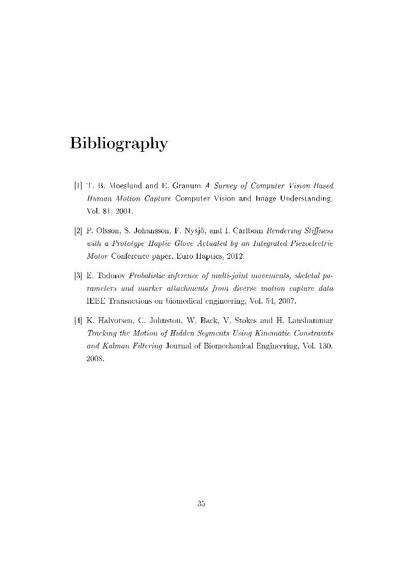
[1] T. B. Moeslund and E. Granum A Survey of Computer Vision-Based
Human Motion Capture Computer Vision and Image Understanding,
Vol. 81, 2001.
[2] P. Olsson, S. Johansson, F. Nysjö, and I. Carlbom Rendering Sti�ness
with a Prototype Haptic Glove Actuated by an Integrated Piezoelectric
Motor Conference paper, Euro Haptics, 2012.
[3] E. Todorov Probalistic inference of multi-joint movements, skeletal pa-
rameters and marker attachments from diverse motion capture data
IEEE Transactions on biomedical engineering, Vol. 54, 2007.
[4] K. Halvorsen, C. Johnston, W. Back, V. Stokes and H. Lanshammar
Tracking the Motion of Hidden Segments Using Kinematic Constraints
and Kalman Filtering Journal of Biomechanical Engineering, Vol. 130,
2008.
35

List of Figures
2.1 The tree describing the kinematic model. . . . . . . . . . . . . 10
2.2 The z-coordinate of the measured position of the marker and
the z-coordinate of the plate. . . . . . . . . . . . . . . . . . . . 15
3.1 The modelled z-coordinate of the index �nger tip and the z-
coordinate of the plate using Method A with ρ = 50 and all
initial values of the states zero. . . . . . . . . . . . . . . . . . 21
3.2 The modelled z-coordinate of the middle �nger tip and the
z-coordinate of the plate using Method A with ρ = 50 and all
initial values of the states zero. . . . . . . . . . . . . . . . . . 21
3.3 The modelled z-coordinate of the index �nger tip and the z-
coordinate of the plate using Method A with ρ = 5 and with
initial values of the states as in table 3.1. . . . . . . . . . . . . 22
3.4 The modelled z-coordinate of the middle �nger tip and the
z-coordinate of the plate using Method A with ρ = 5 and with
initial values of the states as in table 3.1. . . . . . . . . . . . . 22
3.5 The modelled z-coordinate of the index �nger tip and the z-
coordinate of the plate using Method A with ρ = 50 and with
initial values of the states as in table 3.1. . . . . . . . . . . . . 23
3.6 The modelled z-coordinate of the middle �nger tip and the z-
coordinate of the plate using Method A with ρ = 50 and with
initial values of the states as in table 3.1. . . . . . . . . . . . . 23
36
3.7 The modelled z-coordinate of the index �nger tip and the z-
coordinate of the plate using Method A with ρ = 200 and with
initial values of the states as in table 3.1. . . . . . . . . . . . . 24
3.8 The modelled z-coordinate of the middle �nger tip and the
z-coordinate of the plate using Method A with ρ = 200 and
with initial values of the states as in table 3.1. . . . . . . . . . 24
3.9 The modelled z-coordinate of the index �nger tip and the z-
coordinate of the plate using Method B with ω = 0.02. . . . . 26
3.10 The modelled z-coordinate of the middle �nger tip and the
z-coordinate of the plate using Method B with ω = 0.02. . . . 26
3.11 The modelled z-coordinate of the index �nger tip and the z-
coordinate of the plate using Method B with ω = 1. . . . . . . 27
3.12 The modelled z-coordinate of the middle �nger tip and the
z-coordinate of the plate using Method B with ω = 1. . . . . . 27
3.13 The modelled z-coordinate of the index �nger tip and the z-
coordinate of the plate using Method B with ω = 100. . . . . . 28
3.14 The modelled z-coordinate of the middle �nger tip and the
z-coordinate of the plate using Method B with ω = 100. . . . . 28
37