evaluating statistical models: error and inferencecshalizi/uada/12/lectures/ch03.pdfevaluating...

Chapter 3

Evaluating Statistical Models:Error and Inference

3.1 What Are Statistical Models For? Summaries, Fore-casts, Simulators

There are (at least) three levels at which we can use statistical models in data analysis:as summaries of the data, as predictors, and as simulators.

The lowest and least demanding level is just to use the model as a summary of thedata — to use it for data reduction, or compression. Just as one can use the samplemean or sample quantiles as descriptive statistics, recording some features of the dataand saying nothing about a population or a generative process, we could use estimatesof a model’s parameters as descriptive summaries. Rather than remembering all thepoints on a scatter-plot, say, we’d just remember what the OLS regression surfacewas.

It’s hard to be wrong about a summary, unless we just make a mistake. (It may ormay not be helpful for us later, but that’s different.) When we say “the slope whichbest fit the training data was b̂ = 4.02”, we make no claims about anything but thetraining data. It relies on no assumptions, beyond our doing the calculations right.But it also asserts nothing about the rest of the world. As soon as we try to connectour training data to the rest of the world, we start relying on assumptions, and werun the risk of being wrong.

Probably the most common connection to want to make is to say what otherdata will look like — to make predictions. In a statistical model, with random noiseterms, we do not anticipate that our predictions will ever be exactly right, but we alsoanticipate that our mistakes will show stable probabilistic patterns. We can evaluatepredictions based on those patterns of error — how big is our typical mistake? are webiased in a particular direction? do we make a lot of little errors or a few huge ones?

Statistical inference about model parameters — estimation and hypothesis testing— can be seen as a kind of prediction, extrapolating from what we saw in a small

50

3.2. ERRORS, IN AND OUT OF SAMPLE 51

piece of data to what we would see in the whole population, or whole process. Whenwe estimate the regression coefficient b̂ = 4.02, that involves predicting new valuesof the dependent variable, but also predicting that if we repeated the experiment andre-estimated b̂ , we’d get a value close to 4.02.

Using a model to summarize old data, or to predict new data, doesn’t commit usto assuming that the model describes the process which generates the data. But weoften want to do that, because we want to interpret parts of the model as aspects ofthe real world. We think that in neighborhoods where people have more money, theyspend more on houses — perhaps each extra $1000 in income translates into an extra$4020 in house prices. Used this way, statistical models become stories about how thedata were generated. If they are accurate, we should be able to use them to simulatethat process, to step through it and produce something that looks, probabilistically,just like the actual data. This is often what people have in mind when they talk aboutscientific models, rather than just statistical ones.

An example: if you want to predict where in the night sky the planets will be,you can actually do very well with a model where the Earth is at the center of theuniverse, and the Sun and everything else revolve around it. You can even estimate,from data, how fast Mars (for example) goes around the Earth, or where, in thismodel, it should be tonight. But, since the Earth is not at the center of the solarsystem, those parameters don’t actually refer to anything in reality. They are justmathematical fictions. On the other hand, we can also predict where the planets willappear in the sky using models where all the planets orbit the Sun, and the parametersof the orbit of Mars in that model do refer to reality.1

We are going to focus today on evaluating predictions, for three reasons. First,often we just want prediction. Second, if a model can’t even predict well, it’s hardto see how it could be right scientifically. Third, often the best way of checking ascientific model is to turn some of its implications into statistical predictions.

3.2 Errors, In and Out of SampleWith any predictive model, we can gauge how well it works by looking at its errors.We want these to be small; if they can’t be small all the time we’d like them to besmall on average. We may also want them to be patternless or unsystematic (becauseif there was a pattern to them, why not adjust for that, and make smaller mistakes).We’ll come back to patterns in errors later, when we look at specification testing(Chapter 10). For now, we’ll concentrate on how big the errors are.

To be a little more mathematical, we have a data set with points zn = z1, z2, . . . zn .(For regression problems, think of each data point as the pair of input and outputvalues, so zi = (xi , yi ), with xi possibly a vector.) We also have various possible mod-els, each with different parameter settings, conventionally written θ. For regression,θ tells us which regression function to use, so mθ(x) or m(x;θ) is the prediction wemake at point x with parameters set to θ. Finally, we have a loss function L which

1We can be pretty confident of this, because we use our parameter estimates to send our robots to Mars,and they get there.

52 CHAPTER 3. MODEL EVALUATION

tells us how big the error is when we use a certain θ on a certain data point, L(z,θ).For mean-squared error, this would just be

L(z,θ) = (y −mθ(x))2 (3.1)

But we could also use the mean absolute error

L(z,θ) = |y −mθ(x)| (3.2)

or many other loss functions. Sometimes we will actually be able to measure howcostly our mistakes are, in dollars or harm to patients. If we had a model whichgave us a distribution for the data, then pθ(z) would a probability density at z, anda typical loss function would be the negative log-likelihood, − log mθ(z). No matterwhat the loss function is, I’ll abbreviate the sample average of the loss over the wholedata set by L(zn ,θ).

What we would like, ideally, is a predictive model which has zero error on futuredata. We basically never achieve this:

• The world just really is a noisy and stochastic place, and this means even thetrue, ideal model has non-zero error.2 This corresponds to the first, σ2

x , termin the bias-variance decomposition, Eq. 1.26 from Chapter 1.

• Our models are usually more or less mis-specified, or, in plain words, wrong.We hardly ever get the functional form of the regression, the distribution ofthe noise, the form of the causal dependence between two factors, etc., exactlyright.3 This is the origin of the bias term in the bias-variance decomposition.Of course we can get any of the details in the model specification more or lesswrong, and we’d prefer to be less wrong.

• Our models are never perfectly estimated. Even if our data come from a perfectIID source, we only ever have a finite sample, and so our parameter estimatesare (almost!) never quite the true, infinite-limit values. This is the origin ofthe variance term in the bias-variance decomposition. But as we get more andmore data, the sample should become more and more representative of thewhole process, and estimates should converge too.

So, because our models are flawed, we have limited data and the world is stochastic,we cannot expect even the best model to have zero error. Instead, we would like tominimize the expected error, or risk, or generalization error, on new data.

What we would like to do is to minimize the risk or expected loss

E[L(Z ,θ)] =�

d z p(z)L(z,θ) (3.3)

2This is so even if you believe in some kind of ultimate determinism, because the variables we plugin to our predictive models are not complete descriptions of the physical state of the universe, but ratherimmensely coarser, and this coarseness shows up as randomness.

3Except maybe in fundamental physics, and even there our predictions are about our fundamentaltheories in the context of experimental set-ups, which we never model in complete detail.

3.2. ERRORS, IN AND OUT OF SAMPLE 53

To do this, however, we’d have to be able to calculate that expectation. Doing thatwould mean knowing the distribution of Z — the joint distribution of X and Y , forthe regression problem. Since we don’t know the true joint distribution, we need toapproximate it somehow.

A natural approximation is to use our training data zn . For each possible modelθ, we can could calculate the sample mean of the error on the data, L(zn ,θ), calledthe in-sample loss or the empirical risk. The simplest strategy for estimation is thento pick the model, the value of θ, which minimizes the in-sample loss. This strategyis imaginatively called empirical risk minimization. Formally,

�θn ≡ argminθ∈Θ

L(zn ,θ) (3.4)

This means picking the regression which minimizes the sum of squared errors, orthe density with the highest likelihood4. This what you’ve usually done in statisticscourses so far, and it’s very natural, but it does have some issues, notably optimismand over-fitting.

The problem of optimism comes from the fact that our training data isn’t per-fectly representative. The in-sample loss is a sample average. By the law of largenumbers, then, we anticipate that, for each θ,

L(zn ,θ)→ E[L(Z ,θ)] (3.5)

as n→∞. This means that, with enough data, the in-sample error is a good approx-imation to the generalization error of any given model θ. (Big samples are repre-sentative of the underlying population or process.) But this does not mean that thein-sample performance of θ̂ tells us how well it will generalize, because we purposelypicked it to match the training data zn . To see this, notice that the in-sample lossequals the risk plus sampling noise:

L(zn ,θ) = E[L(Z,θ)]+ ηn(θ) (3.6)

Here η(θ) is a random term which has mean zero, and represents the effects of havingonly a finite quantity of data, of size n, rather than the complete probability distribu-tion. (I write it ηn(θ) as a reminder that different values of θ are going to be affecteddifferently by the same sampling fluctuations.) The problem, then, is that the modelwhich minimizes the in-sample loss could be one with good generalization perfor-mance (E[L(Z,θ)] is small), or it could be one which got very lucky (ηn(θ)was largeand negative):

�θn = argminθ∈Θ

�E[L(Z ,θ)]+ ηn(θ)

�(3.7)

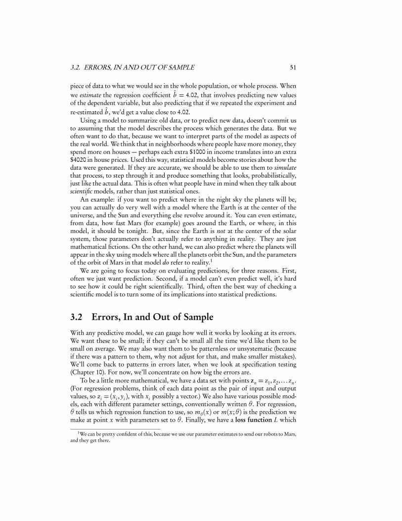
We only want to minimize E[L(Z ,θ)], but we can’t separate it from ηn(θ), so we’realmost surely going to end up picking a �θn which was more or less lucky (ηn < 0)as well as good (E[L(Z ,θ)] small). This is the reason why picking the model whichbest fits the data tends to exaggerate how well it will do in the future (Figure 3.1).

4Remember, maximizing the likelihood is the same as maximizing the log-likelihood, because log isan increasing function. Therefore maximizing the likelihood is the same as minimizing the negative log-likelihood.


0 2 4 6 8 10

24

68

1012

regression slope

MS

E ri

sk

n<-20; theta<-5x<-runif(n); y<-x*theta+rnorm(n)empirical.risk <- function(b) { mean((y-b*x)^2) }true.risk <- function(b) { 1 + (theta-b)^2*(0.5^2+1/12) }curve(Vectorize(empirical.risk)(x),from=0,to=2*theta,xlab="regression slope",ylab="MSE risk")

curve(true.risk,add=TRUE,col="grey")

Figure 3.1: Plots of empirical and generalization risk for a simple case of regressionthrough the origin, Y = θX + ε, ε ∼ � (0,1), with the true θ = 5. X is uniformlydistributed on the unit interval [0,1]. The black curve is the mean squared erroron one particular training sample (of size n = 20) as we vary the guessed slope; herethe minimum is at θ̂ = 5.53. The grey curve is the true or generalization risk. (SeeEXERCISE 2.) The gap between the grey and the black curves is what the text callsηn(θ).

3.3. OVER-FITTING AND MODEL SELECTION 55

Again, by the law of large numbers ηn(θ) → 0 for each θ, but now we need toworry about how fast it’s going to zero, and whether that rate depends on θ. Supposewe knew that minθ ηn(θ) → 0, or maxθ |ηn(θ)| → 0. Then it would follow thatηn(�θn)→ 0, and the over-optimism in using the in-sample error to approximate thegeneralization error would at least be shrinking. If we knew how fast maxθ |ηn(θ)|was going to zero, we could even say something about how much bigger the true riskwas likely to be. A lot of more advanced statistics and machine learning theory isthus about uniform laws of large numbers (showing maxθ |ηn(θ)|→ 0) and rates ofconvergence.

Learning theory is a beautiful, deep, and practically important subject, but alsosubtle and involved one.5 To stick closer to analyzing real data, and to not turn thisinto an advanced probability class, I will only talk about some more-or-less heuristicmethods, which are good enough for many purposes.

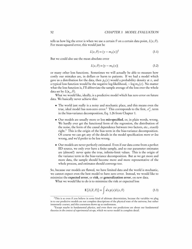
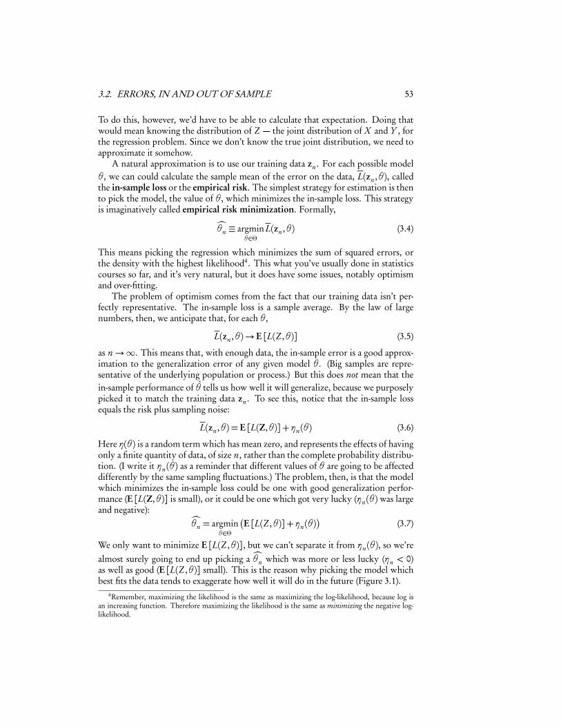
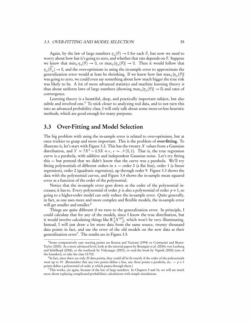
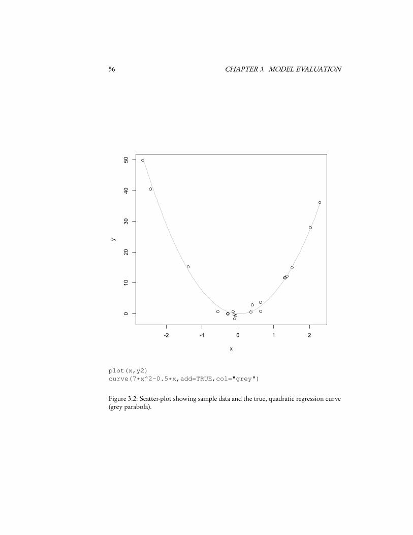
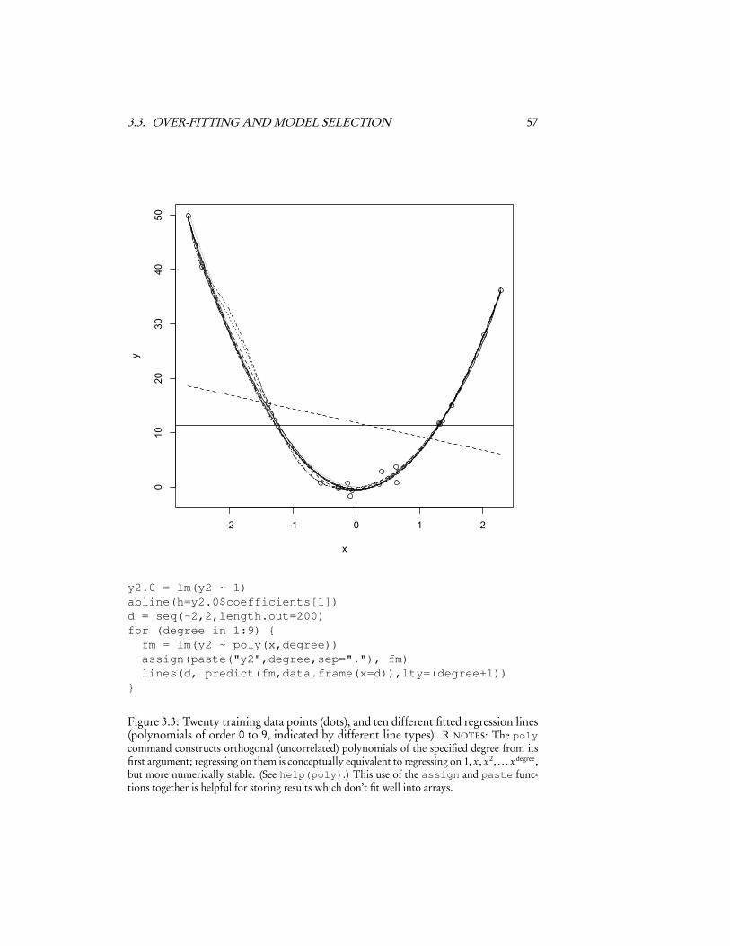
3.3 Over-Fitting and Model SelectionThe big problem with using the in-sample error is related to over-optimism, but atonce trickier to grasp and more important. This is the problem of over-fitting. Toillustrate it, let’s start with Figure 3.2. This has the twenty X values from a Gaussiandistribution, and Y = 7X 2 − 0.5X + ε, ε ∼ � (0,1). That is, the true regressioncurve is a parabola, with additive and independent Gaussian noise. Let’s try fittingthis — but pretend that we didn’t know that the curve was a parabola. We’ll tryfitting polynomials of different orders in x — order 0 (a flat line), order 1 (a linearregression), order 2 (quadratic regression), up through order 9. Figure 3.3 shows thedata with the polynomial curves, and Figure 3.4 shows the in-sample mean squarederror as a function of the order of the polynomial.

Notice that the in-sample error goes down as the order of the polynomial in-creases; it has to. Every polynomial of order p is also a polynomial of order p+1, sogoing to a higher-order model can only reduce the in-sample error. Quite generally,in fact, as one uses more and more complex and flexible models, the in-sample errorwill get smaller and smaller.6

Things are quite different if we turn to the generalization error. In principle, Icould calculate that for any of the models, since I know the true distribution, butit would involve calculating things like E

�X 18�, which won’t be very illuminating.

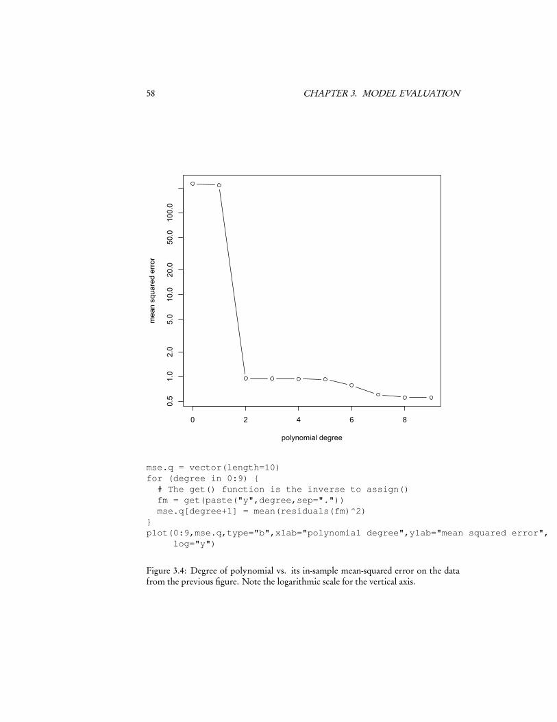
Instead, I will just draw a lot more data from the same source, twenty thousanddata points in fact, and use the error of the old models on the new data as theirgeneralization error7. The results are in Figure 3.5.

5Some comparatively easy starting points are Kearns and Vazirani (1994) or Cristianini and Shawe-Taylor (2000). At a more advanced level, look at the tutorial papers by Bousquet et al. (2004); von Luxburgand Schölkopf (2008), or the textbook by Vidyasagar (2003), or read the book by Vapnik (2000) (one ofthe founders), or take the class 10-702.

6In fact, since there are only 20 data points, they could all be fit exactly if the order of the polynomialswent up to 19. (Remember that any two points define a line, any three points a parabola, etc. — p + 1points define a polynomial of order p which passes through them.)

7This works, yet again, because of the law of large numbers. In Chapters 5 and 16, we will see muchmore about replacing complicated probabilistic calculations with simple simulations.


-2 -1 0 1 2

010

2030

4050

x

y

plot(x,y2)curve(7*x^2-0.5*x,add=TRUE,col="grey")

Figure 3.2: Scatter-plot showing sample data and the true, quadratic regression curve(grey parabola).


-2 -1 0 1 2

010

2030

4050

x

y

y2.0 = lm(y2 ~ 1)abline(h=y2.0$coefficients[1])d = seq(-2,2,length.out=200)for (degree in 1:9) {fm = lm(y2 ~ poly(x,degree))assign(paste("y2",degree,sep="."), fm)lines(d, predict(fm,data.frame(x=d)),lty=(degree+1))

}

Figure 3.3: Twenty training data points (dots), and ten different fitted regression lines(polynomials of order 0 to 9, indicated by different line types). R NOTES: The polycommand constructs orthogonal (uncorrelated) polynomials of the specified degree from itsfirst argument; regressing on them is conceptually equivalent to regressing on 1, x, x2, . . . xdegree,but more numerically stable. (See help(poly).) This use of the assign and paste func-tions together is helpful for storing results which don’t fit well into arrays.


0 2 4 6 8

0.5

1.0

2.0

5.0

10.0

20.0

50.0

100.0

polynomial degree

mea

n sq

uare

d er

ror

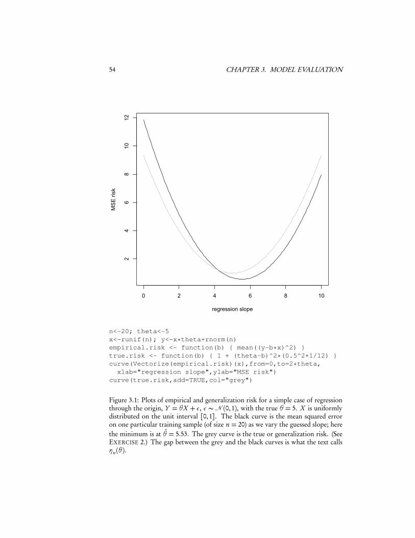
mse.q = vector(length=10)for (degree in 0:9) {# The get() function is the inverse to assign()fm = get(paste("y",degree,sep="."))mse.q[degree+1] = mean(residuals(fm)^2)

}plot(0:9,mse.q,type="b",xlab="polynomial degree",ylab="mean squared error",

log="y")

Figure 3.4: Degree of polynomial vs. its in-sample mean-squared error on the datafrom the previous figure. Note the logarithmic scale for the vertical axis.


0 2 4 6 8

0.5

1.0

2.0

5.0

10.0

20.0

50.0

100.0

polynomial degree

mea

n sq

uare

d er

ror

gmse.q = vector(length=10)for (degree in 0:9) {fm = get(paste("y",degree,sep="."))predictions = predict(fm,data.frame(x=x.new))resids = y.new - predictionsgmse.q[degree+1] = mean(resids^2)

}plot(0:9,mse.q,type="b",xlab="polynomial degree",

ylab="mean squared error",log="y",ylim=c(min(mse.q),max(gmse.q)))lines(0:9,gmse.q,lty=2,col="blue")points(0:9,gmse.q,pch=24,col="blue")

Figure 3.5: In-sample error (black dots) compared to generalization error (blue trian-gles). Note the logarithmic scale for the vertical axis.


What is happening here is that the higher-order polynomials — beyond order 2 —are not just a bit optimistic about how well they fit, they are wildly over-optimistic.The models which seemed to do notably better than a quadratic actually do much,much worse. If we picked a polynomial regression model based on in-sample fit, we’dchose the highest-order polynomial available, and suffer for it.

What’s going on here is that the more complicated models — the higher-orderpolynomials, with more terms and parameters — were not actually fitting the general-izable features of the data. Instead, they were fitting the sampling noise, the accidentswhich don’t repeat. That is, the more complicated models over-fit the data. In termsof our earlier notation, η is bigger for the more flexible models. The model whichdoes best here is the quadratic, because the true regression function happens to be ofthat form. The more powerful, more flexible, higher-order polynomials were able toget closer to the training data, but that just meant matching the noise better. In termsof the bias-variance decomposition, the bias shrinks with the model order, but thevariance of estimation grows.

Notice that the models of order 0 and order 1 also do worse than the quadraticmodel — their problem is not over-fitting but under-fitting; they would do better ifthey were more flexible. Plots of generalization error like this usually have a mini-mum. If we have a choice of models — if we need to do model selection — we wouldlike to find the minimum. Even if we do not have a choice of models, we might liketo know how big the gap between our in-sample error and our generalization erroris likely to be.

There is nothing special about polynomials here. All of the same lessons applyto variable selection in linear regression, to k-nearest neighbors (where we need tochoose k), to kernel regression (where we need to choose the bandwidth), and toother methods we’ll see later. In every case, there is going to be a minimum for thegeneralization error curve, which we’d like to find.

(A minimum with respect to what, though? In Figure 3.5, the horizontal axis isthe model order, which here is the number of parameters (minus one). More gener-ally, however, what we care about is some measure of how complex the model spaceis, which is not necessarily the same thing as the number of parameters. What’s morerelevant is how flexible the class of models is, how many different functions it canapproximate. Linear polynomials can approximate a smaller set of functions thanquadratics can, so the latter are more complex, or have higher capacity. More ad-vanced learning theory has a number of ways of quantifying this, but the details arepretty arcane, so we will just use the concept of complexity or capacity informally.)

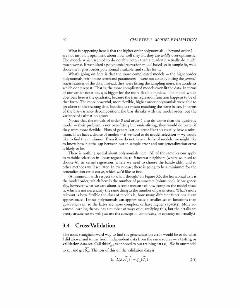
3.4 Cross-ValidationThe most straightforward way to find the generalization error would be to do whatI did above, and to use fresh, independent data from the same source — a testing orvalidation data-set. Call this z�m , as opposed to our training data zn . We fit our model

to zn , and get�θn . The loss of this on the validation data is

E�

L(Z ,�θn)�+ η�m(�θn) (3.8)

3.4. CROSS-VALIDATION 61

where now the sampling noise on the validation set, η�m , is independent of�θm . So thisgives us an unbiased estimate of the generalization error, and, if m is large, a preciseone. If we need to select one model from among many, we can pick the one whichdoes best on the validation data, with confidence that we are not just over-fitting.

The problem with this approach is that we absolutely, positively, cannot use anyof the validation data in estimating the model. Since collecting data is expensive — ittakes time, effort, and usually money, organization and skill — this means getting avalidation data set is expensive, and we often won’t have that luxury.

3.4.1 Data-set SplittingThe next logical step, however, is to realize that we don’t strictly need a separatevalidation set. We can just take our data and split it ourselves into training and testingsets. If we divide the data into two parts at random, we ensure that they have (asmuch as possible) the same distribution, and that they are independent of each other.Then we can act just as though we had a real validation set. Fitting to one part ofthe data, and evaluating on the other, gives us an unbiased estimate of generalizationerror. Of course it doesn’t matter which half of the data is used to train and whichhalf is used to test, so we can do it both ways and average.

Figure 3.6 illustrates the idea with a bit of the data and linear models from thefirst homework set, and Code Example 1 shows the code used to make Figure 3.6.

3.4.2 k-Fold Cross-Validation (CV)The problem with data-set splitting is that, while it’s an unbiased estimate of the risk,it is often a very noisy one. If we split the data evenly, then the test set has n/2data points — we’ve cut in half the number of sample points we’re averaging over. Itwould be nice if we could reduce that noise somewhat, especially if we are going touse this for model selection.

One solution to this, which is pretty much the industry standard, is what’s calledk-fold cross-validation. Pick a small integer k, usually 5 or 10, and divide the dataat random into k equally-sized subsets. (The subsets are sometimes called “folds”.)Take the first subset and make it the test set; fit the models to the rest of the data, andevaluate their predictions on the test set. Now make the second subset the test setand the rest of the training sets. Repeat until each subset has been the test set. At theend, average the performance across test sets. This is the cross-validated estimate ofgeneralization error for each model. Model selection then picks the model with thesmallest estimated risk.8

The reason cross-validation works is that it uses the existing data to simulate theprocess of generalizing to new data. If the full sample is large, then even the smallerportion of it in the training data is, with high probability, fairly representative of thedata-generating process. Randomly dividing the data into training and test sets makes

8A closely related procedure, sometimes also called “k-fold CV”, is to pick 1/k of the data points atrandom to be the test set (using the rest as a training set), and then pick an independent 1/k of the datapoints as the test set, etc., repeating k times and averaging. The differences are subtle, but what’s describedin the main text makes sure that each point is used in the test set just once.


MedianHouseValue MedianIncome MedianHouseAge1 452600 8.3252 412 358500 8.3014 213 352100 7.2574 524 341300 5.6431 525 342200 3.8462 526 269700 4.0368 52



�βintercept�βincome�βage MSE

Income only 44607.2 42061.4 NA 7.13× 109

Income + Age -13410.9 43509.2 1825.6 6.61× 109

�βintercept�βincome�βage MSE

Income only 45576.9 41523.1 NA 6.89× 109

Income + Age -6974.14 42826.72 1662.85 6.45× 109

MSE(1→ 2) MSE(2→ 1) averageIncome only 6.88× 109 7.14× 109 7.01× 109

Income + Age 6.46× 109 6.62× 109 6.54× 109

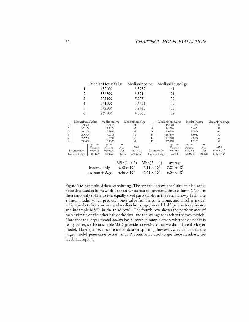
Figure 3.6: Example of data-set splitting. The top table shows the California housing-price data used in homework 1 (or rather its first six rows and three columns). This isthen randomly split into two equally sized parts (tables in the second row). I estimatea linear model which predicts house value from income alone, and another modelwhich predicts from income and median house age, on each half (parameter estimatesand in-sample MSE’s in the third row). The fourth row shows the performance ofeach estimate on the other half of the data, and the average for each of the two models.Note that the larger model always has a lower in-sample error, whether or not it isreally better, so the in-sample MSEs provide no evidence that we should use the largermodel. Having a lower score under data-set splitting, however, is evidence that thelarger model generalizes better. (For R commands used to get these numbers, seeCode Example 1.

3.4. CROSS-VALIDATION 63

head(calif[,1:3])which.half <- sample(rep(1:2,length.out=nrow(calif)))head(calif[which.half==1,1:3])head(calif[which.half==2,1:3])small.1 <- lm(MedianHouseValue~MedianIncome,data=calif[which.half==1,])

small.2 <- lm(MedianHouseValue~MedianIncome,data=calif[which.half==2,])

large.1 <- lm(MedianHouseValue~MedianIncome+MedianHouseAge,data=calif[which.half==1,])

large.2 <- lm(MedianHouseValue~MedianIncome+MedianHouseAge,data=calif[which.half==2,])

in.sample.mse <- function(fit) { mean(fit$residuals^2) }in.sample.mse(small.1)in.sample.mse(large.1)in.sample.mse(small.2)in.sample.mse(large.2)cross.sample.mse <- function(fit,half) {test <- calif[which.half != half,]return(mean((test$MedianHouseValue

- predict(fit,newdata=test))^2))}cross.sample.mse(small.1,2)cross.sample.mse(small.2,1)cross.sample.mse(large.1,2)cross.sample.mse(large.2,1)

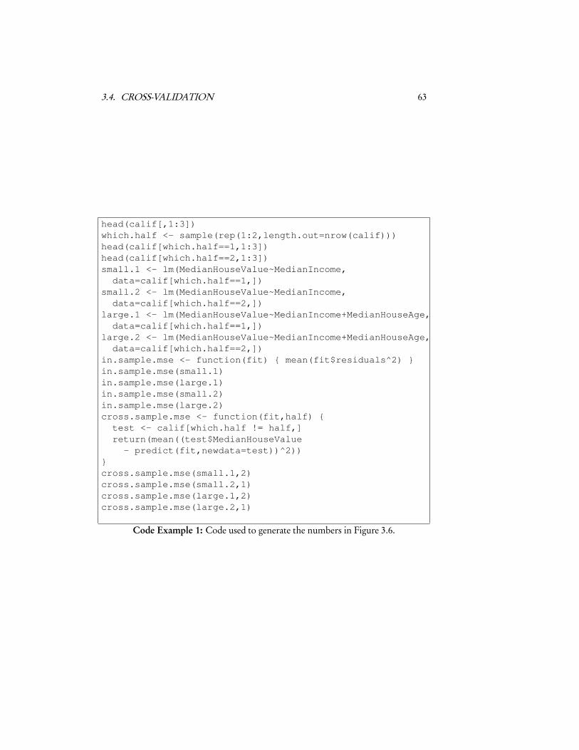
Code Example 1: Code used to generate the numbers in Figure 3.6.


it very unlikely that the division is rigged to favor any one model class, over and abovewhat it would do on real new data. Of course the original data set is never perfectlyrepresentative of the full data, and a smaller testing set is even less representative,so this isn’t ideal, but the approximation is often quite good. It is especially good atgetting the relative order of different models right, that is, at controlling over-fitting.9

Cross-validation is probably the most widely-used method for model selection,and for picking control settings, in modern statistics. There are circumstances whereit can fail — especially if you give it too many models to pick among — but it’s thefirst thought of seasoned practitioners, and it should be your first thought, too. Thehomework to come will make you very familiar with it.

3.4.3 Leave-one-out Cross-Validation

Suppose we did k-fold cross-validation, but with k = n. Our testing sets wouldthen consist of single points, and each point would be used in testing once. This iscalled leave-one-out cross-validation. It actually came before k-fold cross-validation,and has two advantages. First, it doesn’t require any random number generation, orkeeping track of which data point is in which subset. Second, and more importantly,because we are only testing on one data point, it’s often possible to find what theprediction on the left-out point would be by doing calculations on a model fit to thewhole data. This means that we only have to fit each model once, rather than k times,which can be a big savings of computing time.

The drawback to leave-one-out CV is subtle but often decisive. Since each trainingset has n − 1 points, any two training sets must share n − 2 points. The models fitto those training sets tend to be strongly correlated with each other. Even thoughwe are averaging n out-of-sample forecasts, those are correlated forecasts, so we arenot really averaging away all that much noise. With k-fold CV, on the other hand,the fraction of data shared between any two training sets is just k−2

k−1 , not n−2n−1 , so even

though the number of terms being averaged is smaller, they are less correlated.There are situations where this issue doesn’t really matter, or where it’s over-

whelmed by leave-one-out’s advantages in speed and simplicity, so there is certainlystill a place for it, but one subordinate to k-fold CV.10

3.5 Warnings

Some caveats are in order.

9The cross-validation score for the selected model still tends to be somewhat over-optimistic, becauseit’s still picking the luckiest model — though the influence of luck is much attenuated. Tibshirani andTibshirani (2009) provides a simple correction.

10At this point, it may be appropriate to say a few words about the Akaike information criterion, orAIC. AIC also tries to estimate how well a model will generalize to new data. One can show that, understandard assumptions, as the sample size gets large, leave-one-out CV actually gives the same estimate asAIC (Claeskens and Hjort, 2008, §2.9). However, there do not seem to be any situations where AIC workswhere leave-one-out CV does not work at least as well. So AIC should really be understood as a very fast,but often very crude, approximation to the more accurate cross-validation.

3.5. WARNINGS 65

1. All of these model selection methods aim at getting models which will gen-eralize well to new data, if it follows the same distribution as old data. Gener-alizing well even when distributions change is a much harder and much lesswell-understood problem (Quiñonero-Candela et al., 2009). It is particularlytroublesome for a lot of applications involving large numbers of human be-ings, because society keeps changing all the time — it’s natural for the variablesto vary, but the relationships between variables also change. (That’s history.)

2. All the model selection methods we have discussed aim at getting models whichpredict well. This is not necessarily the same as getting the true theory of theworld. Presumably the true theory will also predict well, but the converse doesnot necessarily follow. We will see examples later where false but low-capacitymodels, because they have such low variance of estimation, actually out-predictcorrectly specified models.

3.5.1 Parameter InterpretationThe last item is worth elaborating on. In many situations, it is very natural to wantto attach some substantive, real-world meaning to the parameters of our statisticalmodel, or at least to some of them. I have mentioned examples above like astronomy,and it is easy to come up with many others from the natural sciences. This is also ex-tremely common in the social sciences. It is fair to say that this is much less carefullyattended to than it should be.

To take just one example, consider the paper “Luther and Suleyman” by Prof.Murat Iyigun (Iyigun, 2008). The major idea of the paper is to try to help explainwhy the Protestant Reformation was not wiped out during the European wars ofreligion (or alternately, why the Protestants did not crush all the Catholic powers),leading western Europe to have a mixture of religions, with profound consequences.Iyigun’s contention is that all of the Christians were so busy fighting the OttomanTurks, or perhaps so afraid of what might happen if they did not, that conflicts amongthe European Christians were suppressed. To quote his abstract:

at the turn of the sixteenth century, Ottoman conquests lowered thenumber of all newly initiated conflicts among the Europeans roughlyby 25 percent, while they dampened all longer-running feuds by morethan 15 percent. The Ottomans’ military activities influenced the lengthof intra-European feuds too, with each Ottoman-European military en-gagement shortening the duration of intra-European conflicts by morethan 50 percent.

To back this up, and provide those quantitative figures, Prof. Iyigun estimates linearregression models, of the form11

Yt =β0+β1Xt +β2Zt +β3Ut + εt (3.9)

where Yt is “the number of violent conflicts initiated among or within continentalEuropean countries at time t”12, Xt is “the number of conflicts in which the Ottoman

11His Eq. 1 on pp. 1473; I have modified the notation to match mine.12In one part of the paper; he uses other dependent variables elsewhere.


Empire confronted European powers at time t”, Zt is “the count at time t of thenewly initiated number of Ottoman conflicts with others and its own domestic civildiscords”, Ut is control variables reflecting things like the availability of harvests tofeed armies, and εt is Gaussian noise.

The qualitative idea here, about the influence of the Ottoman Empire on theEuropean wars of religion, has been suggested by quite a few historians before13. Thepoint of this paper is to support this rigorously, and make it precise. That supportand precision requires Eq. 3.9 to be an accurate depiction of at least part of the processwhich lead European powers to fight wars of religion. Prof. Iyigun, after all, wants tobe able to interpret a negative estimate ofβ1 as saying that fighting off the Ottomanskept Christians from fighting each other. If Eq. 3.9 is inaccurate, if the model is badlymis-specified, however, β1 becomes the best approximation to the truth within asystematically wrong model, and the support for claims like “Ottoman conquestslowered the number of all newly initiated conflicts among the Europeans roughly by25 percent” drains away.

To back up the use of Eq. 3.9, Prof. Iyigun looks at a range of slightly differentlinear-model specifications (e.g., regress the number of intra-Christian conflicts thisyear on the number of Ottoman attacks last year), and slightly different methods ofestimating the parameters. What he does not do is look at the other implicationsof the model: that residuals should be (at least approximately) Gaussian, that theyshould be unpredictable from the regressor variables. He does not look at whetherthe relationships he thinks are linear really are linear (see Chapters 4, 8, and 10). Hedoes not try to simulate his model and look at whether the patterns of Europeanwars it produces resemble actual history (see Chapter 16). He does not try to checkwhether he has a model which really supports causal inference, though he has a causalquestion (see Part III).

I do not say any of this to denigrate Prof. Iyigun. His paper is actually much betterthan most quantitative work in the social sciences. This is reflected by the fact that itwas published in the Quarterly Journal of Economics, one of the most prestigious, andrigorously-reviewed, journals in the field. The point is that by the end of this course,you will have the tools to do better.

3.6 ExercisesTo think through, not to hand in.

1. Suppose that one of our model classes contains the true and correct model, butwe also consider more complicated and flexible model classes. Does the bias-variance trade-off mean that we will over-shoot the true model, and always gofor something more flexible, when we have enough data? (This would meanthere was such a thing as too much data to be reliable.)

2. Derive the formula for the generalization risk in the situation depicted in Fig-ure 3.1, as given by the true.risk function in the code for that figure. Inparticular, explain to yourself where the constants 0.52 and 1/12 come from.

13See §1–2 of Iyigun (2008), and MacCulloch (2004, passim).

evaluating statistical models: error and inferencecshalizi/uada/12/lectures/ch03.pdfevaluating...

Documents