evaluating real mortgage mitigation options · evaluating real mortgage mitigation options abstract...

Evaluating Real Mortgage

Mitigation Options

Michael Flanagan*

Manchester Metropolitan University, UK

March 29, 2013

Submitted for ROC Tokyo, July 2013

JEL Classifications: C73, D81, G32

Keywords: Property, Delinquency, Double Trigger Default, Options, Capital Structure

Acknowledgements: We thank Stuart Hyde, Ser-Huang Poon, and Richard Stapleton for helpful comments on an

earlier version.

2

Evaluating Real Mortgage Mitigation Options

Abstract

We provide an appropriate comprehensive model for assessing the likely contribution

of current US government programs to alleviate homeownership financial distress. In

a simulation of five available mortgage distress termination options plus continuation

and repayment, the HAMP program appears to foster mortgage mitigation, given our

parameter value assumptions, primarily through enabling and encouraging voluntary

house sales. However, conclusive policy appraisal awaits satisfactory empirical work.

3

Introduction

It is clear that a significant number of US homeowners, due to exogenous shocks, are unable

to make required monthly mortgage payments (Holden et al. 2012, Quercia, Pennington-Cross

and Tian 2012). This is an important consideration in the current US economic climate, as

Federal mitigation programs such as the Home Affordable Mortgage Program (HAMP) are

designed to mitigate this inability of homeowners to make the required debt servicing

payments. The fact that these programs address the homeowner’s ability to pay rather than

their willingness to pay implies that generally accepted outcomes from option theoretic

simulation models which rely heavily (Vandell 1995) on a perpetual ability to pay assumption

should be re-examined. Does the homeowner’s inability to pay affect the probability and

value of foreclosure, strategic default or other alternative option?

Our analysis is based on exogenous program criteria for entry to the Home Affordable

Mortgage Program (HAMP) (SIGTARP 2010), which primarily lowers homeowner’s debt

servicing to income ratios (DTI). The program thereby aims to make mortgage payments of

homeowners with a high debt burden more affordable by encouraging renegotiation between

lender and homeowner, mitigating the effects of other (undesirable) options such as

foreclosure or default.

We simulate the relative importance (defined by the likelihood of exercise) of the principal

alternative options based on the HAMP program acceptance criteria. The main benefit of

entry to the HAMP program for the homeowner is that they negotiate and receive a one off

reduction in their mortgage payment for a period of 5 years resulting in a DTI close to a

recommended value of 0.31. In effect, we simulate (and interpret the results) for a complex

mixture of discrete (time) compound, barrier and reset type options.

4

This paper develops a model around a problem formulation based on exogenous HAMP entry

criteria, incorporating the stochastic factors (LTV and DTI), to provide an insight into the

relative likelihood of different mitigation options being exercised. The DTI ratio compares a

homeowner’s required debt payments (primarily interest and amortization) to the monthly-

earned income. The loan-to-value (LTV) ratio expresses the amount of a first mortgage lien as

a percentage of the total appraised value of the property. We compare three scenarios: (i) a

homeowner’s income and equity value is rising and no HAMP type program exists; (ii) a

homeowner’s income and equity value is falling and a HAMP type program is not available,

(iii) or a HAMP program is available.

We comment on the expected effect of a HAMP type program on the more typical mitigation

options such as a “forced foreclosure” or “strategic default” as well as additional real options

introduced by the relaxation of the perpetual ability to pay constraint such as a “voluntary

sale”. We demonstrate that a possible effect of the HAMP program is that it makes it less

likely that a typical US homeowner will default because of “unwillingness to pay” but rather,

willingly, will sell their home because of an inability to pay and the desire to recover some

home equity. Appendix 1 contains a more detailed description of these options.

The DTI criteria generate options, which are equivalent to a path dependent barrier option,

with reset and subsequently continuing default or restoration options. Barrier options are one

of the oldest types of exotic options trading since 1967 on the Chicago Board of Options

Exchange (Zhang 1998). As a result, literature on exotic barrier options is abundant (Zhang

1998, Wilmott 2006). Snyder (1969) outlined the general approach with a single stochastic

variable and a lower barrier, which was later extended, to multiple stochastic variables and

barriers of different forms and durations (Heynen and Kat 1994, 1996).

5

However, examination of the literature has not yielded specific research or papers, which lend

themselves to a closed form solution of the particular problem as described in section 2.

Wilmott (2006) suggests that a Monte Carlo methodology is often the best approach with

regard to analysing exotic path dependent options, as it is simple to code with a likelihood of

fewer mistakes and whose only disadvantages are the difficulty of obtaining the Greeks and

its slowness, both of which are minor issues in our formulation. This view is also supported

by Vandell (1995) when discussing specific problem formulations associated with an

extension of the standard option theoretic problem from a bivariate stochastic formulation.

To illustrate the methodological complexity we make the following observations about our

specific formulation. It is a discrete Asian option (monthly), as significant errors might be

introduced by treating it as a continuous time option (Zhang 1998). Our formulation might

appear at first sight to be a simple bivariate option with LTV and DTI as independent

variables but this is not so as DTI and LTV combine in a sequential or compound manner

(double trigger action) to knock out the mortgage and trigger a terminal payoff option. Our

problem is also less straight forward than many barrier options treated in the literature as in

our specific case the homeowner’s DTI is reset to 0.31 (but the LTV is not reset) on hitting

the HAMP reset barrier of 0.38.

We also consider the appropriateness of treating both DTI and LTV as standard geometric

Brownian motion (gBm) processes. This assumption is relatively uncontroversial for LTV

(Vandell 1995) but may be open to discussion in relation to DTI and the underlying income

dynamics. Income dynamics are difficult to simulate, and the measurement and interpretation

of US homeowner income dynamics are even more fraught than the measurement of property

values and subject to many caveats. Recent empirical research by Quercia, Pennington-Cross

6

and Tian (2012) suggest that DTI for low and moderate-income US households is in the first

instance symmetrically distributed with a bell shaped distribution.

An examination of literature on US homeowner income dynamics (e.g. Gottschalk and

Moffitt 2009; Dynan, Elmendorf and Sichel 2007) does not provide evidence that other

formulations, such as mean reverting (income), are more widely used or provide any better

results than the simpler standard gBm. Although a homeowner’s income may revert over the

longer term this is of no consequence to the homeowner or lender who are faced with short to

medium term payment difficulties. The HAMP program also has a relatively short duration of

5 years leading us to choose a standard gBm stochastic process.

Section 2 discusses the model and methodology. Section 3 provides some provisional results

based on assumed exogenous trigger levels and parameter values. Finally, section 4 concludes

and points to the empirical work required for policy evaluation.

7

2 Model and Methodology

The purpose of the analysis is to consider and estimate the effect entry to the HAMP program

might have on the probability of how often common real mortgage default mitigation options

available to US homeowners might be exercised.

We formulate the problem by defining five real competing mortgage mitigation options

(Appendix 1) to occur with a probability of 1 within the term of the mortgage. We follow up

by stating the path dependent (on LTV and DTI) assumptions as to when each option is

exercised. Finally, we describe the mitigation effect of the HAMP program within the

problem formulation, make assumptions as to how the path dependency of the five competing

options are modified (or mitigated) and compare the relative probability of a mitigating option

being exercised to a state of the world without a HAMP program.

The Probability of a Terminal Mortgage Option Occurring

The probability of a competing event terminating the term of a mortgage is 1:

P (Strategic Default) + P (Forced Foreclosure) + P (Paid Up) + P (Voluntary Sale) = 1 - P (Other Option) (1)

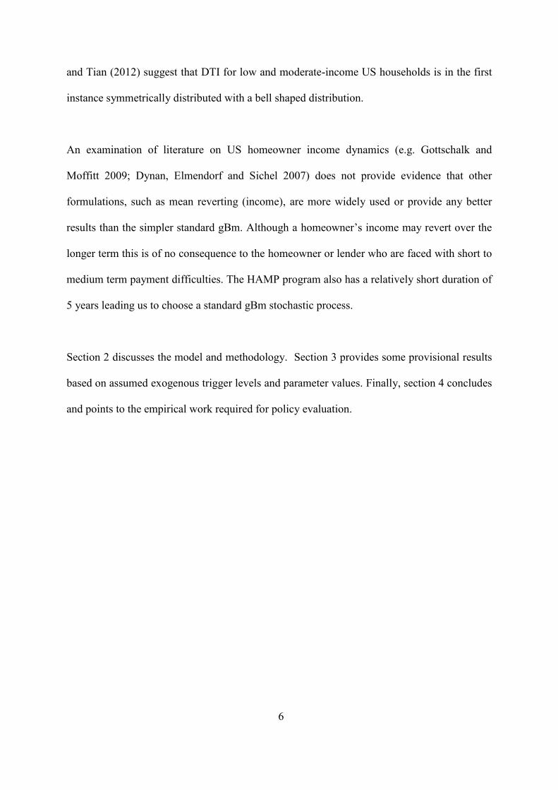
We present this concept in a diagrammatic manner in Figure 1 which shows that a US

homeowner who experiences stochastic LTV and DTI over the term of their mortgage must

hit one of the termination boundaries or remain within the boundaries (= Other Option). To

the right of some arbitrary DTI value X (Can’t Pay) a homeowner will either, as a result, of an

inability to pay, be foreclosed upon if they have negative equity or voluntary sell their home if

they have positive equity. Above some arbitrary LTV value Y (Won’t Pay), a homeowner will

strategically default no matter their DTI. Otherwise the homeowner, who still has the ability

8

to pay, will either have a mortgage that is paid up or still current (= other option). A typical

US homeowner with a prime mortgage starts with a DTI of around 0.2 and LTV of 80% (= P,

yellow star) in the diagram. Sub-prime mortgages start closer to the right (= SP, red star) and

may have a higher probability of other termination events occurring.

Figure 1. Schematic of Alternative US Mitigation Options without HAMP

9

Therefore if DTI is an independent random variable in the set 0 < DTI < ∞ and LTV is

another uncorrelated independent variable in the set 0 < LTV < ∞, X and Y are arbitrarily

chosen boundaries and a homeowner has either positive or negative equity (defined as ≤ or >

100%).

We suggest that:

P(Strategic Default) ≡ P(LTV ≥ Y | 0 < DTI < ∞) +

P(Voluntary Sale) ≡ P(LTV ≤ 100% | DTI ≥ X) +

P(Paid Up) ≡ P(LTV < 1% | 0 <DTI < ∞) +

P(Forced Foreclosure) ≡ P(LTV >100% | DTI ≥ X) =

1- P(Other Option) ≡ 1- P(1% < LTV < X | 0 < DTI < X) (2)

The effect of the HAMP program is represented pictorially in Figure 2 overleaf whereby US

homeowners who have a DTI > 0.38 or LTV > 110% can negotiate with their lender, enter

HAMP and have their DTI reduced to 0.31. HAMP is a temporary mitigating option and does

not offer a permanent reduction in DTI, as homeowner DTI and LTV will then change

subsequent to entering the program. However, it is obvious that entering the HAMP will

affect the relative probabilities of any of the terminal options expressed in (2) being exercised.

10

Figure 2. Schematic of Alternative US Mitigation Options with HAMP

As discussed in the introduction, an appropriate approach for this particular problem

formulation is to simulate, using a Monte Carlo approach, the effect of stochastic LTV (a

measure of the homeowner’s equity in their property) and DTI (a measure of the ability to

make the monthly payment) on the exercise likelihood of a US homeowner’s mortgage

options.

Firstly, the ability of the homeowner to pay must be checked (1st

DTI Trigger) and only

subsequently the willingness of the homeowner to pay (2nd

LTV Trigger) – a so called double

trigger. If the first trigger shows that the homeowner has the ability to pay, then the available

real options reduce to those of strategic default, paid up and other option. However, if the

homeowner is unable to pay, then two other real options are introduced namely, the lender

forecloses or the homeowner voluntarily sells the property.

11

We introduce an additional feature into our simulation model whereby a mortgage event is not

immediately triggered if one of the stochastic factors e.g. DTI (ability to pay) hits a threshold

value in one period but only if it consistently exceeds the threshold for a number of periods.

This is not a continuous but rather a discrete time simulation with discrete monthly time

periods. Treating a model as discrete time rather than continuous time introduces large

differences in exercise probability (Zhang, 1998). This feature simply reflects the accepted

fact that lenders and homeowners do not generally exercise an option immediately in the

period following the first missed payment or reduction in home equity.

We make no assumption about the amount of the monthly payment beyond that a repayment

formula or schedule is contractually agreed beforehand and that failure by the homeowner to

make the agreed payment on time constitutes a trigger event changing their mortgage status.

Let be the number of (monthly) periods over which the homeowner

discovers their “true” DTI and “true” LTV respectively before exercising a mortgage option.

Let = a unique US residential owner occupied mortgage homeowner where and

= number of homeowners in the simulation. We let years be the term of the

mortgage and the number of payment periods implying monthly payments.

Implicit in this model formulation is that both the homeowner’s DTI and LTV processes are

significant, independent and non-correlated. Mortgage literature (Campbell and Dietrich

1983, Vandell and Thibodeau 1985) does not contradict this view as empirical research has

demonstrated that these two factors are highly significant but essentially independent.

12

The DTI Factor

This measure is of prime importance and significance within the US mortgage industry as its

initial value at origination and consequent development gives lenders an idea of how likely it

is that the homeowner will be able to repay the loan over its full term. We do not make any

distinction within our model as to why DTI is changing being a result of variations in both

income and/or housing expenses. The change in housing expenses could be due to any

number of reasons ranging from interest rate changes to property taxes or mortgage insurance.

During more normal times, most US lender underwriting standards tended to adopt a value of

0.28 as a maximum upper limit for DTI at mortgage initiation. We adopt 0.18 for DTI at

mortgage origination for the majority of our simulations, a value considered more normal for

prime mortgages. Our exogenous triggers are motivated by the following considerations.

We assume (Holden et al. 2012, Quercia, Pennington-Cross and Tian 2012) that a homeowner

will have serious ability to pay issues if their DTI is above 0.5 for at least three consecutive

payment periods and will most likely be foreclosed upon. The HAMP program applies a

maximum limit of 0.38 to a homeowner’s DTI that is reduced to 0.31 using a waterfall

method (Holden et al. 2012) on successful entry to the program.

We assume that the DTI of any homeowner , denoted by D, follows the simple gBm

process given by

(3)

is the instantaneous expected rate of change of the DTI ratio

is the instantaneous variance of the DTI ratio

is a standard Brownian motion.

We make the simplifying assumption that all homeowners have the same , and .

13

The LTV Factor

We again take a simple approach and assume that the LTV is a result of many factors. With

no change in property price, for the majority of homeowners the LTV will gradually decrease

from month to month as they pay down the loan principal. For others, due to any number of

reasons varying from non-payment of principal to a reduction in property prices the LTV may

be static or increase. The LTV is only appraised (precisely) once at mortgage initiation and

again by the lender or servicing agent in the event of default. Otherwise, the LTV is

calculated by the homeowner and lender based on the outstanding principal and arrears as

well as a very rough estimation of the property price based on local (if known) property prices

or indexes. In the US, conforming loans that meet Fannie Mae and Freddie Mac underwriting

guidelines are limited to an LTV ratio that is less than or equal to 80% at origination which

value we assume in the simulation model.

Our exogenous triggers are motivated by the following considerations. We define a higher

LTV trigger of 150% in our model as the boundary where a homeowner will decide to

“strategically” default because of the payoff received by putting the mortgage against the

value of the property collateral. The 150 % LTV is consistent with empirical papers by

Gerardi, Foote and Willen (2008) or Guiso, Sapienza and Zingales (2009). We also include a

lower boundary where LTV < 1% where the mortgage is effectively paid down and

terminated.

A relatively wide range of homeowners are eligible to participate in the HAMP program

based on equity or LTV criteria ranging from those with a small percentage of positive equity

(LTV > 90%) up to those with negative equity (LTV < 110%). We note that the HAMP

programs LTV criteria were recently increased again in June 2012 to 120% (Holden et al.

14

2012). Currently the 120% limit is one that has been adopted within the HAMP program as a

“typical” LTV break point (Holden et al 2012) although we have adopted the lower 110%

barrier, basing our analysis on the original HAMP criteria.

We assume that if the homeowner has the ability to pay (< 0.5 DTI for three consecutive

periods), that where the homeowner’s LTV is above 110% for the same three consecutive

periods, they will enter and participate in the HAMP program as an alternative to strategically

defaulting.

As discussed in the introduction, we assume that the LTV of any homeowner , denoted by

L, follows the gBm process given by

(4)

Where

is the instantaneous expected rate of change of the LTV ratio

is the instantaneous variance of the LTV ratio

is a standard Brownian motion.

We make the simplifying assumption that all homeowners have the same , and , and

there is no correlation between L and D.

The Interaction of LTV and DTI – the Double Trigger Effect

We summarise the alternative mitigation options available to the homeowner as well as the

program logic of the exercise barriers in Table 1. We assume that initially a homeowner is not

in a HAMP program. At the end of each monthly period, first the DTI is simulated and

compared to the DTI trigger, then the LTV is simulated and compared to the LTV trigger.

15

Should any of the conditions described in Table 1 (No HAMP Program) persist for longer

than 3 months then that particular terminal option is triggered. If the government then

introduces a HAMP program and the homeowner meets the entry criteria as specified in Table

1 (With a HAMP Program) then the homeowner enters HAMP and their status changes from

0 to 1 and DTI is reset to 0.31. They then are subject to the same periodical simulation (as

without a HAMP Program (Table 1, Whereupon) and do not qualify for a DTI reset again.

Table 1. Exogenous Trigger Values for the Option Simulation Program

HAMP Status 1st DTI Trigger 2nd LTV Trigger Option Description

No HAMP Program

IF AND THEN

0 DTI < 0.5 1% < LTV < 150% Other Option

0 DTI < 0.5 LTV ≤ 1% Paid Up

0 DTI < 0.5 LTV ≥ 150% Strategic Default

0 DTI ≥ 0.5 LTV < 100% Voluntary Sale

0 DTI ≥ 0.5 LTV ≥ 100% Foreclosure

With a HAMP Program

IF OR THEN

0 -> 1 DTI ≥ 0.38 LTV ≥ 110% Enter HAMP => DTI Resets to 0.31

Whereupon

IF AND THEN

1 DTI < 0.5 1% < LTV < 150% Other Option

1 DTI < 0.5 LTV ≤ 1% Paid Up

1 DTI < 0.5 LTV ≥ 150% Strategic Default

1 DTI ≥ 0.5 LTV < 100% Voluntary Sale

1 DTI ≥ 0.5 LTV ≥ 100% Foreclosure

Note: An option is triggered only if DTI or LTV are at a trigger level for at least consecutive three monthly periods

16

3 Simulated Results and Interpretation

We initially study a US homeowner with a prime mortgage at origination (DTI=0.18 and

LTV = 81%): a worst case (economic) scenario where the DTI and LTV increase at a rate of

2% per year and a best case scenario where LTV and DTI are decreasing by 2% per year. We

assume that no HAMP type program is available in the best-case scenario but is introduced in

a worst-case type scenario. Note that in a deterministic world, in the worst case the LTV hits

a zero net equity position in the 12th

year, but the DTI never becomes high enough to qualify

for HAMP, as shown in Figure 2A.

Figure 2A Deterministic Evolution of DTI and LTV under a Worse Case Scenario of +2%.

It is apparent that the substantial trigger in the worst case scenario is going to be regarding the

LTV, but of course in a stochastic world, the DTI may also be hit early with some positive

probability.

0

0.2

0.4

0.6

0.8

1

1.2

1.4

1.6

0 1 2 3 4 5 6 7 8 9 10 11 12 13 14 15 16 17 18 19 20 21 22 23 24 25 26 27 28 29 30

DT

I a

nd

LT

V

Period

DTI

LTV

17

We take the same global approach to analysing each individual terminal option.

1) We compare the percentage of homeowners who exercise with a HAMP type program

to a state of the world without a HAMP type program for different volatility

parameters.

2) We estimate the terminal change in LTV and DTI from mortgage origination. This

indicates (but does not quantify) whether entry to the HAMP program “preserves” or

“destroys” LTV (a measure of equity) for the homeowner.

3) We examine the seasoning effect of how many homeowners exercise within 5 years

and for those who enter HAMP, re-examine how effective the program has been in

preventing or delaying a subsequent foreclosure, sale or default over the next 5 years.

We demonstrate the effect of the model initially on the exercise probability of the foreclosure

option in detail. Detailed numerical and graphical information on the foreclosure and other

options are available from the authors.

Foreclosure Option – Volatility Effects

Foreclosure occurs when a homeowner’s income (modelled by DTI) is not sufficient to make

the monthly payment and there is no equity (modelled by LTV) in their property whereby a

voluntary sale (or downsizing) would pay off the loan. The y axis of the four subplots in

Figure 3 represents the percentage of homeowners who have the foreclosure option exercised

against themselves. The x axis of the top two subplots respectively worse and best case

represents the LTV ( ) volatility while the x axis on the bottom two subplots represents DTI

( ) volatility.

18

Figure 3 Percentage Homeowners Foreclosing as a Function of LTV ( ) and DTI ( ) Volatility

We show four trend lines in each subplot. In the top two subplots, representing the percentage

of homeowners exercising foreclosure plotted against LTV ( ) volatility, we show trend lines

for DTI ( ) = 20% (dashed trend line) and 40% (continuous trend line). In the bottom two

subplots representing the percentage of homeowners exercising foreclosure plotted against

DTI ( ) volatility we show trend lines for LTV ( ) = 20% (dashed trend line) and 40%

(continuous trend line). Red lines represent results without any (NO) HAMP program – the

status quo in good economic times. Black lines represent results when a HAMP type program

is available.

Worst Case Best Case

Worst Case Best Case

Simulation Parameters

σl , μl , μl , σd , μd , μd = Variable, Delay Trigger for DTI and LTV=3 months, Term Period = 360 months, Strategic Default LTV Trigger = 150%

Voluntary Sales DTI Trigger = 0.5, HAMP DTI Trigger = 0.38, HAMP DTI Reset = 0.31, HAMP LTV Trigger = 110%, Number of Householders = 100,000

19

We see by comparing the two left hand sub plots to the two right hand sub plots that

foreclosures decrease as the homeowner’s economic circumstances improve. Foreclosures

increase (nearly) linearly with increasing DTI volatility (bottom two subplots) due to the

increased likelihood of hitting the inability to pay trigger.

In contrast, with increasing LTV volatility (top two subplots) foreclosures decrease at

moderate to high levels of LTV volatility. Increasing LTV volatility therefore offers some

homeowners the opportunity to benefit from increased positive equity and reduces the

likelihood of foreclosure. Lower LTV volatility, on the other hand reduces the likelihood that

a homeowner with negative equity will ever have positive equity.

It should be noted that some other homeowners are more likely as a result to exercise the

strategic default option at these higher LTV volatilities. In contrast to other mitigation

options, little change in the percentage of homeowners exercising this option occurs at higher

LTV volatility but all the “action” takes place at low to moderate levels of LTV volatility.

Table 2, column 2 summarises (for , = 20% and 40%) the percentage (of N=100,000)

homeowners exercising a particular option during the best and worst cases depicted in Figure

3. The right hand sub table is the best-case scenario i.e. where LTV and DTI are decreasing

by 2% a year and the left hand sub table is the worst-case scenario where LTV and DTI are

increasing by 2% a year. Each individual sub table summarises the percentage number of

homeowners who exercise one of 6 options – numbered 1-6. The top half of each sub table

give the results for a HAMP program and the bottom half for NO HAMP program. Finally

results are presented for combinations of LTV and DTI volatility with , = 20% and 40%.

20

Table 2 Effect of LTV ( ) and DTI ( ) Volatility on Homeowner Option Exercise Frequency

From Table 2 (best case, column 2) which summarises key parameters from the simulations

for a LTV ( ) and DTI ( ) volatility of 20%, approximately 0.94% of homeowners will be

foreclosed upon in a best-case scenario without a HAMP program (NH). When the

homeowner’s economic situation worsens (worse case, column 2) this increases to 3.71 %

without a HAMP program (NH) but reaches 6.79% with a HAMP program (H). The

introduction of a HAMP program would not, in the first instance, lead to reduced

foreclosures. The forbearance that some homeowners enjoy from a reduced DTI is in many

cases only a temporary reprieve, whereby once the homeowner has recurring income or debt

difficulties the LTV has turned either negative triggering a forced foreclosure instead of a

voluntary sale or positive triggering a voluntary sale instead of a forced foreclosure.

Voluntary Sales Option – Volatility Effects

Voluntary sales occur when the homeowner’s DTI is not sufficient to make the periodic

payment over a three-month period but enough positive equity (as determined by LTV) exists

in the property to allow a voluntary sale. We analyse the voluntary sales option in a similar

σl σd 1 2 3 4 5 6

H 0.2 0.2 17.3 2.14 19.8 42.3 1.63 24.3

0.4 27.7 5.86 16.1 36.3 1.3 25.1

H 0.4 0.2 14.7 0.77 32.9 17.1 25.8 14.9

0.4 24.7 3 29.3 14.6 21.7 17.6

NH 0.2 0.2 7.64 0.94 21.6 68.2 1.63 0

0.4 16.6 2.61 19.7 59.6 1.49 0

NH 0.4 0.2 6.03 0.41 34.8 29.8 29 0

0.4 14.1 1.63 32.6 26.2 25.4 0

Best Case Scenario μd= μl= -0.02

σl σd 1 2 3 4 5 6

H 0.2 0.2 28.8 6.79 39.4 16.6 0.16 24.7

0.4 30.9 11.3 32.8 16.8 0.14 27.6

H 0.4 0.2 28.5 1.9 41.2 12.2 10.7 17.5

0.4 30.2 4.48 36.8 12.6 10.4 19.9

NH 0.2 0.2 17.3 3.71 45.4 33.4 0.2 0

0.4 20.4 5.55 41.6 32.3 0.18 0

NH 0.4 0.2 16.6 1.28 44.9 23.7 13.5 0

0.4 19.3 2.71 42.4 23.1 12.4 0

Worst Case Scenario μd= μl= 0.02


Delay Trigger for DTI and LTV=3 months, Term Period = 360 months, Strategic Default LTV Trigger = 150%, H =HAMP Program, NH = NO HAMP program, σl and σd = 20% or 40%


Column Option Descriptions : Percentage Homeowners who 1 = Voluntarily Sell, 2 = Forceclose, 3 = Strategically Default, 4 = Other Option, 5 = Paid Up, 6 = Enter HAMP

21

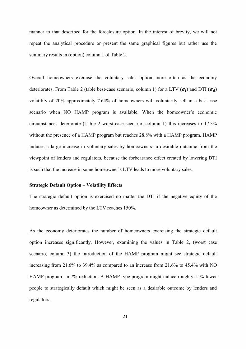
manner to that described for the foreclosure option. In the interest of brevity, we will not

repeat the analytical procedure or present the same graphical figures but rather use the

summary results in (option) column 1 of Table 2.

Overall homeowners exercise the voluntary sales option more often as the economy

deteriorates. From Table 2 (table best-case scenario, column 1) for a LTV ( ) and DTI ( )

volatility of 20% approximately 7.64% of homeowners will voluntarily sell in a best-case

scenario when NO HAMP program is available. When the homeowner’s economic

circumstances deteriorate (Table 2 worst-case scenario, column 1) this increases to 17.3%

without the presence of a HAMP program but reaches 28.8% with a HAMP program. HAMP

induces a large increase in voluntary sales by homeowners- a desirable outcome from the

viewpoint of lenders and regulators, because the forbearance effect created by lowering DTI

is such that the increase in some homeowner’s LTV leads to more voluntary sales.

Strategic Default Option – Volatility Effects

The strategic default option is exercised no matter the DTI if the negative equity of the

homeowner as determined by the LTV reaches 150%.

As the economy deteriorates the number of homeowners exercising the strategic default

option increases significantly. However, examining the values in Table 2, (worst case

scenario, column 3) the introduction of the HAMP program might see strategic default

increasing from 21.6% to 39.4% as compared to an increase from 21.6% to 45.4% with NO

HAMP program - a 7% reduction. A HAMP type program might induce roughly 15% fewer

people to strategically default which might be seen as a desirable outcome by lenders and

regulators.

22

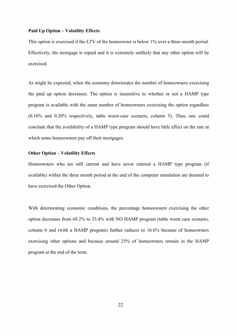
Paid Up Option – Volatility Effects

This option is exercised if the LTV of the homeowner is below 1% over a three-month period.

Effectively, the mortgage is repaid and it is extremely unlikely that any other option will be

exercised.

As might be expected, when the economy deteriorates the number of homeowners exercising

the paid up option decreases. The option is insensitive to whether or not a HAMP type

program is available with the same number of homeowners exercising the option regardless

(0.16% and 0.20% respectively, table worst-case scenario, column 5). Thus, one could

conclude that the availability of a HAMP type program should have little effect on the rate at

which some homeowners pay off their mortgages.

Other Option – Volatility Effects

Homeowners who are still current and have never entered a HAMP type program (if

available) within the three month period at the end of the computer simulation are deemed to

have exercised the Other Option.

With deteriorating economic conditions, the percentage homeowners exercising the other

option decreases from 68.2% to 33.4% with NO HAMP program (table worst case scenario,

column 6 and (with a HAMP program) further reduces to 16.6% because of homeowners

exercising other options and because around 25% of homeowners remain in the HAMP

program at the end of the term.

23

How Much Does LTV and DTI Change Conditional on the Option Exercised?

We now address our second analytical question to discover what effect the introduction of a

HAMP program has on the average change in LTV and DTI from mortgage origination

compared to a NO HAMP scenario. This might help increase our understanding of whether

homeowners who enter HAMP experience beneficial changes in DTI or LTV from a scenario

where NO HAMP program is available? Strictly speaking, rational homeowners should only

be motivated by future expectations but it is not unreasonable to assume, that notwithstanding

HAMP benefits and lender forbearance, that the average US homeowner may compare

terminal LTV to LTV at origination. Similarly, rational lenders should only be interested in

NPV (Holden et al.2012) but may also be concerned with managing loan losses and interested

in the net change in LTV of their mortgage loans and customer’s DTI from origination.

We assume that the difference in LTV between mortgage origination and the exercise of a

terminal option such as strategic default, forced foreclosure or voluntary sale gives a measure

of the change in equity to the homeowner (and therefore lender). The difference, depending

on the type of option, can be negative and positive as demonstrated in the histogram of the

change in LTV from mortgage origination in Figure 4 for a simulation of 100,000 US

homeowners in a worst case scenario with HAMP.

Figure 4 Change in LTV from Mortgage Origination for those Exercising the Voluntary Sale Option


Delay Trigger for DTI and LTV=3 months, Term Period = 360 months, Strategic Default LTV Trigger = 150%


Worse Case = μd = μl = 0.02, , H =HAMP Program, σl = σd = 20%, LTV0 = 81%, DTI0 = 0.18

24

We construct the voluntary sales histogram by selecting those homeowners who exercise the

option (at the reference volatilities). We divide these homeowners into LTV “buckets” across

a (change in LTV) range from -100% to +100%. We finally numerically integrate the area to

calculate the mean change in LTV from origination for those homeowners. We report the

mean of the changes in LTV (and similarly for DTI) in Table 3 for the voluntary sale, forced

foreclosure and strategic default options.

Table 3 Homeowners Option Exercise Frequency and Average Change in LTV and DTI from to.

Voluntarily Sale Option – LTV Effects

For we calculate (table 3 sub-table 2 column 1) a mean change in LTV of -

33.8% in the best case No HAMP situation, -23.6% in the worst case NO HAMP situation

and -20.4% in the worst case HAMP situation. Homeowners who exercise the voluntary sale

option after entering a HAMP type program have a LTV that is on average 3.2% higher at

option exercise compared to when NO HAMP is available.

Although LTV and DTI is increasing for both the HAMP and NO HAMP cases in the worst

case scenario, because the homeowner “hangs in” longer by entering the HAMP program and

gaining the DTI reset benefit, they also “lose” more equity due to a higher LTV at

termination.


Delay Trigger for DTI and LTV=3 months, Term Period = 360 months, Strategic Default LTV Trigger = 150%, H =HAMP Program, NH = NO HAMP program


Worse Case = μd = μl = 0.02, Best Case = μd = μl = -0.02, σl = σd = 20% or 40%,LTV0 = 81%, DTI0 = 0.18

Column Option Descriptions : Percentage Homeowners who 1 = Voluntarily Sell, 2 = Forceclose, 3 = Strategically Default

25

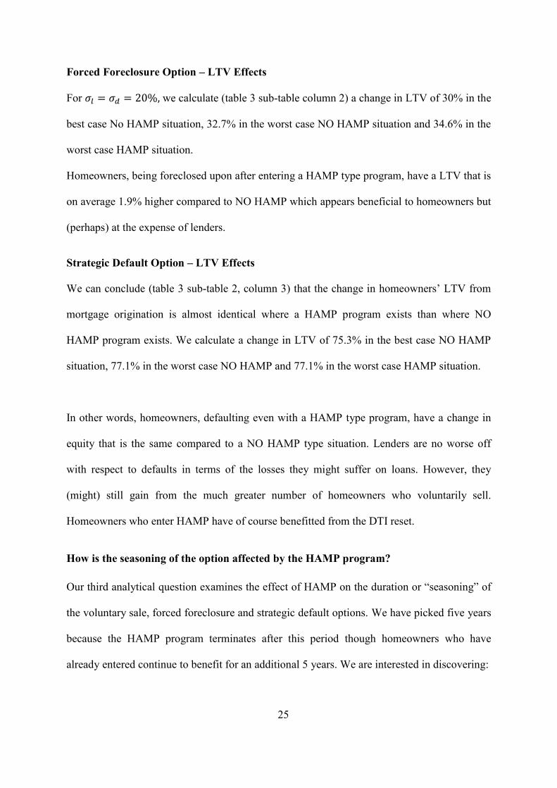
Forced Foreclosure Option – LTV Effects

For we calculate (table 3 sub-table column 2) a change in LTV of 30% in the

best case No HAMP situation, 32.7% in the worst case NO HAMP situation and 34.6% in the

worst case HAMP situation.

Homeowners, being foreclosed upon after entering a HAMP type program, have a LTV that is

on average 1.9% higher compared to NO HAMP which appears beneficial to homeowners but

(perhaps) at the expense of lenders.

Strategic Default Option – LTV Effects

We can conclude (table 3 sub-table 2, column 3) that the change in homeowners’ LTV from

mortgage origination is almost identical where a HAMP program exists than where NO

HAMP program exists. We calculate a change in LTV of 75.3% in the best case NO HAMP

situation, 77.1% in the worst case NO HAMP and 77.1% in the worst case HAMP situation.

In other words, homeowners, defaulting even with a HAMP type program, have a change in

equity that is the same compared to a NO HAMP type situation. Lenders are no worse off

with respect to defaults in terms of the losses they might suffer on loans. However, they

(might) still gain from the much greater number of homeowners who voluntarily sell.

Homeowners who enter HAMP have of course benefitted from the DTI reset.

How is the seasoning of the option affected by the HAMP program?

Our third analytical question examines the effect of HAMP on the duration or “seasoning” of

the voluntary sale, forced foreclosure and strategic default options. We have picked five years

because the HAMP program terminates after this period though homeowners who have

already entered continue to benefit for an additional 5 years. We are interested in discovering:

26

a) How many homeowners who (eventually) exercise a particular option enter the

HAMP program within the first five years?

b) How many of these homeowners in a) who enter the HAMP program eventually

exercise the same option in the following 5 years?

The simulation program notes the period when the homeowner enters the HAMP program and

then the period when the homeowner subsequently exercises one of the terminal options –

strategic default, forced foreclosure or a voluntary sale. We plot histograms of duration effects

for the different options and then integrate and summarise key data from the histograms for

three types of options - strategic default, voluntary sales and forced foreclosures, in Table 4.

By way of example only, the left hand subplot in Figure 5 below answers question a) while

the right hand subplot answers question b) for voluntary sale.

Figure 5 Histograms of Homeowners who Voluntary Sell as a Function of Entry Time and Program Status


Delay Trigger for DTI and LTV=3 months, Term Period = 360 months, Strategic Default LTV Trigger = 150%


Worse Case = μd = μl = 0.02, H =HAMP Program, σl = σd = 20% , LTV0= 80%, DTI0 = 0.21

27

Table 4 LTV Change, Durations and Exercise Frequency for Prime Homeowners.

Voluntary Sale Option – Seasoning Effect

We simulate (row 1, voluntary sale column) for N=100000 that the number of homeowners

who exercise the voluntary sale option over the 30 years term as 8883 (best case/NO HAMP),

21595 (worse case/NO HAMP) and 33622 (worse case/HAMP). i.e. HAMP increases

voluntary sales absolutely.

Row 2 (table) and the left hand plot (Figure 4) shows that of the 33622 who enter HAMP,

23% (or 7733) exercise the voluntary sale option within the first 5 years which answers a).

With NO HAMP program although 21595 homeowners eventually voluntary sell, only 9%

(1943) of these do so within the first five years of a 30 year term.

Under HAMP, 8735 (row 3) of those voluntarily selling (33622) will at some time (not

necessarily in the first 5 years) enter the program whereby 61% of these 8735 (i.e. 5328 of the

7733) will have entered within the first 5 years of their 30-year mortgage term. Of those 8735

that enter, 36% will nevertheless voluntarily sell within 5 years of entering HAMP which

answers part b) above.

Option Description ---> Strategic Default Forced Foreclosure Voluntary Sales

Economic Case ----> Best Worse Worse Best Worse Worse Best Worse Worse

Program Type ----> NH NH H NH NH H NH NH H

Number of homeowners who exercise over 30 years 18787 43355 37767 757 4440 6437 8883 21595 33622

Percentage of those who exercise within 5 years of t0 23% 22% 25% 18% 14% 16% 9% 9% 23%

Number of homeowners entering Hamp 1647 5942 8735

Percentage of those entering Hamp within 5 years of t0 51% 58% 61%

Percentage of those who enter and exercise in + 5 years 55% 69% 36%

Mean Change in LTV from t0 85% 85% 85% 86% 38% 41% 43% 42% 35% -24% -21% -10%


Delay Trigger for DTI and LTV=3 months, Term Period = 360 months, Strategic Default LTV Trigger = 150%,H =HAMP Program, NH = NO HAMP program


Worse Case = μd = μl = 0.02, Best Case = μd = μl = -0.02, σl = σd = 20% , LTV0= 80%, DTI0 = 0.21

28

We conclude that the HAMP program is particularly effective when compared in the next two

sub sections to the foreclosure and strategic default options in “steering” prime mortgage

holders towards a voluntary sale within a short time period of initiating their mortgage but not

necessarily in delaying the exercise of the voluntary sale option for a third of this group.

The mean decrease in LTV of the 8735 HAMP homeowners voluntarily selling is 10%

compared to a mean decrease of 21% for the total 33622 homeowners who voluntarily sell

over the 30-year term (row 4). In contrast to those other (voluntary sales) homeowners who

did not enter the HAMP program, HAMP homeowners are significantly worse off when they

eventually sell their homes, which reflects the fact that LTV is increasing over the period.

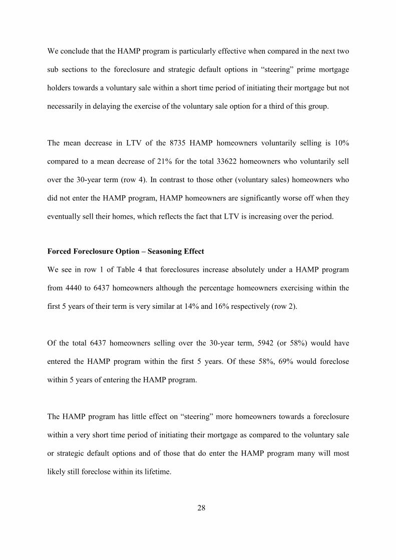
Forced Foreclosure Option – Seasoning Effect

We see in row 1 of Table 4 that foreclosures increase absolutely under a HAMP program

from 4440 to 6437 homeowners although the percentage homeowners exercising within the

first 5 years of their term is very similar at 14% and 16% respectively (row 2).

Of the total 6437 homeowners selling over the 30-year term, 5942 (or 58%) would have

entered the HAMP program within the first 5 years. Of these 58%, 69% would foreclose

within 5 years of entering the HAMP program.

The HAMP program has little effect on “steering” more homeowners towards a foreclosure

within a very short time period of initiating their mortgage as compared to the voluntary sale

or strategic default options and of those that do enter the HAMP program many will most

likely still foreclose within its lifetime.

Prime

Homeowner

s

29

Examining the change in LTV since origination, we note that the mean change in LTV is

43%, which is 2% higher than the worst-case scenario without a HAMP program. In other

words, on average, individual prime mortgage holders who foreclose appear to be slightly

“better off” in terms of their equity position if a HAMP program is available in that they can

“put” a lower value property/higher loan to the lender. In addition, they have benefitted from

the DTI reset. Lenders are therefore “losing” on average.

Strategic Default Option – Seasoning Effect

The number of homeowners who exercise the strategic default option over the 30 years term

is 43355 (worse case/NO HAMP) compared to 37767 (worse case/HAMP). In contrast to the

other two options, HAMP reduces strategic defaults absolutely.

When a HAMP program is available 1647 of those defaulting will enter HAMP at some time

within their 30 year mortgage term of which 51% will be within the first 5 years. Of those

1647 that enter, 55% will nevertheless strategically default within 5 years of entering HAMP.

We make the important conclusion that the HAMP program does not necessarily “steer”

prime mortgage holders towards a strategic default within a very short time period of

initiating their mortgage but that the majority will nevertheless still strategically default

within a 5 year period.

Examining the change in LTV since origination we note that the mean change in LTV is 85%

which is the same as in a worst case scenario without a HAMP program. Those subprime

mortgage homeowners who enter the HAMP program on average have a change of LTV of

86% and are therefore only slightly “better off” when they put their property to the lender but

will have enjoyed some benefit from the DTI reset.

30

4. Conclusion

We conclude by summing up the main findings at our reference volatilities of , = 20%.

We examine the simulated effect of a HAMP program on real mortgage mitigation options

and by extension answer our research objective of whether ignoring the ability to pay of

homeowners is justified by its effect on strategic default and foreclosure. We repeat that the

outcomes of the HAMP program are very dependent on the initial LTV and DTI at

origination. Therefore, for the typical US homeowner with a DTI of 0.18 and LTV of 81%:

1) A HAMP type program leads to a significant increase in homeowners exercising the

voluntary sales option from 17.3% to 28.8% - a desirable outcome from the viewpoint

of homeowners, lenders and regulators due to the (presumed) reduced associated

deadweight costs. This occurs because the temporary mitigation effect created by

lowering the DTI of homeowners is such that the positive development of some

homeowner’s LTV due to higher volatility induces more voluntary sales. This

conclusion might however be difficult to verify empirically as it is probably not easy

to divine homeowners’ motivations for selling.

2) Forced foreclosures double during the lifetime of a HAMP program from 3.7% to

6.7%. The forbearance that homeowners enjoy from a reduced DTI will in many cases

be only a temporary reprieve whereby once the homeowner has recurring income or

debt difficulties the LTV has turned either negative forcing a foreclosure instead of a

voluntary sale or positive permitting a voluntary sale instead of a foreclosure. This

conclusion is more easily verifiable. However, opponents of the (hand out) program

may claim that the program has therefore failed.

31

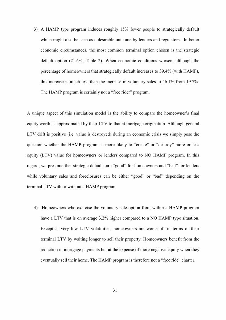
3) A HAMP type program induces roughly 15% fewer people to strategically default

which might also be seen as a desirable outcome by lenders and regulators. In better

economic circumstances, the most common terminal option chosen is the strategic

default option (21.6%, Table 2). When economic conditions worsen, although the

percentage of homeowners that strategically default increases to 39.4% (with HAMP),

this increase is much less than the increase in voluntary sales to 46.1% from 19.7%.

The HAMP program is certainly not a “free rider” program.

A unique aspect of this simulation model is the ability to compare the homeowner’s final

equity worth as approximated by their LTV to that at mortgage origination. Although general

LTV drift is positive (i.e. value is destroyed) during an economic crisis we simply pose the

question whether the HAMP program is more likely to “create” or “destroy” more or less

equity (LTV) value for homeowners or lenders compared to NO HAMP program. In this

regard, we presume that strategic defaults are “good” for homeowners and “bad” for lenders

while voluntary sales and foreclosures can be either “good” or “bad” depending on the

terminal LTV with or without a HAMP program.

4) Homeowners who exercise the voluntary sale option from within a HAMP program

have a LTV that is on average 3.2% higher compared to a NO HAMP type situation.

Except at very low LTV volatilities, homeowners are worse off in terms of their

terminal LTV by waiting longer to sell their property. Homeowners benefit from the

reduction in mortgage payments but at the expense of more negative equity when they

eventually sell their home. The HAMP program is therefore not a “free ride” charter.

32

5) Homeowners, being foreclosed upon from after entering a HAMP type program, have

a LTV that is on average 1.9% higher compared to a NO HAMP type situation.

Lenders are consequently slightly worse off with respect to foreclosures in terms of

the losses they might suffer on loans. However, this is compensated by their gain from

the much greater number of homeowners who voluntarily sell.

6) With respect to the strategic default option, a homeowners’ average terminal LTV is

almost identical after entry to the HAMP program than where NO HAMP program

exists. Lenders are no worse off with respect to strategic defaults in terms of the losses

they might suffer on loans. However, they still gain from the much greater number of

homeowners who voluntarily sell. It is a moot point whether the homeowner will take

the presence of a HAMP program into account when considering their strategic default

decision. On the other hand, they will gladly make use of any DTI reduction. It

remains difficult for regulators or lenders to design a mitigation program where

strategic defaulters do not attempt to game to their own advantage.

We conclude by summarising the seasoning or duration effect of a HAMP program on the

exercise frequency of prime mortgage homeowners.

7) HAMP seems particularly effective in “steering” prime mortgage holders towards a

voluntary sale within a short time of initiating their mortgage. However these

homeowners are significantly worse off in terms of the change in LTV from

origination when they eventually sell their homes.

33

8) The HAMP program does little to reduce foreclosures within the 5-year lifetime of the

HAMP program, in contrast to its effect on the voluntary sale option.

9) The HAMP program is not effective in “steering” prime mortgage holders away from

strategic defaulting. Only a small number of these types of homeowners enter HAMP

as would be expected from the HAMP application criteria and most of those entering

will still “ruthlessly” default.

These form the main conclusions from our study of how we might expect terminal options

such as voluntary sales, foreclosure and strategic default to behave in the medium to longer

term given the presence of a HAMP type program.

The main effect using this model is that a HAMP program steers more US homeowners

towards a voluntary sale and slightly reduces the number of defaults and foreclosures. This

outcome, depending on deadweight default costs, is most likely to be advantageous to US

homeowners and lenders. Overall, many homeowners who enter HAMP still end up

exercising a (generally more favourable) terminal option within the typical 5 years HAMP

duration.

Unfortunately, the two main options in percentage terms, affected by the HAMP program,

voluntary sales and strategic default, are notoriously difficult to measure empirically. It will

remain difficult for opponents and supporters of the HAMP program to conclusively assess its

benefit to US society. We have demonstrated that, given the program’s cost ($50 billion) and

the immediate benefit to distressed US homeowners, with a significant increase in voluntary

34

sales and reduction of defaults with the consequent reduction in default deadweight costs, it is

probably better to have a HAMP program in place rather than having NO HAMP program.

Finally, we return to our main research question as to whether the ability to pay assumption is

valid or not. On balance, we have not demonstrated that ignoring the ability to pay of

residential homeowners is invalid when examining the strategic default option only. However,

we can argue as a result of our simulation that where the foreclosure option is of interest then

one must consider both stochastic DTI and LTV and that the ability to pay assumption is

invalid. This is because traditional option theoretic modelling focuses narrowly on the

strategic default and foreclosure options to the exclusion of alternative options. In this sense,

introducing a stochastic DTI parameter mainly effects the voluntary sale option which is

ignored by the traditional approach focussing on LTV. Stochastic DTI has less effect on

strategic default which is influenced mainly by LTV but does affect foreclosures.

There are many areas for future research, extending or supplementing this study. First, there

are numerous simulations which have not been shown, or interpreted, between the worst and

best cases, and for sub-prime mortgages. Secondly, the current model is based on DTI and

LTV, not on a specific type of mortgage with a stochastic I and V, which may be correlated.

Thirdly, no attempt has been made so far to value the HAMP program, or the multiple options

available, as in Azevedo-Pereira et al. (2002) and Daglish and Patel (2012). Finally, the

conclusions and evaluation of the HAMP program await adequate empirical inputs.

35

References

Azevedo-Pereira, J.S., D.P. Newton and D.A. Paxson (2002), U.K. Fixed-Rate Repayment

Mortgage and Mortgage Indemnity Valuation, Real Estate Economics 30: 185-211.

Campbell, T. and J. Dietrich (1983), The Determinants of Default on Conventional

Residential Mortgages, Journal of Finance, 38(5):1569-1581.

COP (2009), Foreclosure Crisis: Working Toward a Solution, Congressional Oversight

Panel, Publication No. 110-343.

Daglish, T. and N. Patel (2012), Fixed Come Hell or High Water? Selection and Prepayment

of Fixed-Rate Mortgages Outside the United States. Real Estate Economics 40: 709-744.

Das, S.R. and R. Meadows (2010), Strategic Loan Modification: An Options-Based Response

to Strategic Default, Working Papers SCU.

Geradi, K..,A. Shapiro and P.S. Willen (2008), Subprime Mortgages: Risky Mortgages,

HomeOwnership Experiences and Foreclosure, Federal Reserve Bank of Boston, Working

Paper No 07-15.

Gottschalk, P and R. Moffitt (2009), The Rising Instability of U.S. Earnings, Journal of

Economic Perspectives, 23:4 Fall 2009: 3-24

Guiso, L., P. Sapienza and L. Zingales (2009), Moral and Social Constraints in Strategic

Default on Mortgages, EUI Working Paper, ECO 2009/27.

36

HAMP Website (2012),http://www.makinghomeaffordable.gov/Pages/default.aspx

Heynen, R and H. Kat (1996), Brick by Brick, Risk, 9(6).

Heynen, R and H. Kat (1994), Partial Barrier Options, Journal of Financial Engineering,

3(3/4): 253-274.

Holden, S., A. Kelly, D. McManus, T. Scharlemann, R. Singer and J. D. Worth (2012), The

HAMP NPV Model: Development and Early Performance, Real Estate Economics, 40:32-64.

(OTS) Office of Thrift Supervision US Department of the Treasury (2011), OCC and OTS

Mortgage Metrics Report 4th

Q 2010, http://www.ots.treas.gov/_files/490069.pdf

Quercia, R.G., A. Pennington-Cross and C.Y. Tian (2012), Mortgage Default and Prepayment

Risks among Moderate- and Low-Income Households, Real Estate Economics, 40:159-198.

SIGTARP (2010), Factors Affecting Implementation of the HOME Affordable Modification

Program, Washington SIGTARP-10-005March 25.

Snyder, G.L. (1969), Alternative Forms of Options, Financial Analysts Journal, 25:93-99.

Vandell, K.D. (1995), How Ruthless is Mortgage Default: A Review and Synthesis of the

Evidence, Journal of Housing Research, 6:245-264.

http://www.ots.treas.gov/_files/490069.pdf

37

Vandell, K and T. Thibodeau (1985), Estimation of Mortgage Defaults Using Disaggregate

Loan History Data, Journal of the American Real Estate and Urban Economics

Association,13(3):292-316.

Wilmott, P. (2006), Quantitative Finance, Wiley London.

Zhang, P. G. (1998), Exotic Options: A Guide to Second Generation Options, World

Scientific Singapore.

38

Appendix 1

Forced Foreclosure

Forced foreclosure occurs when a homeowner does not have sufficient income, as determined

by DTI, to make the required monthly payment to the lender. We assume that the homeowner

has no savings or other means of paying down the loan. Furthermore, the LTV or

homeowner’s equity is negative such that a voluntary sale is of no interest to the homeowner

or lender. The option is triggered by the lender if the homeowner is delinquent over a number

of monthly periods.

Voluntary Sale

Voluntary sale occurs when a homeowner does not have sufficient income, as determined by

DTI, to make the monthly payment to the lender. We assume that the homeowner has no

savings or other means of paying down the loan. However, in contrast to the forced

foreclosure option, enough positive equity exists in the property to make a voluntary sale

attractive to the borrower as the least worse option.

Strategic Default

Strategic default occurs where a homeowner considers that the amount of negative equity in

the property as determined by LTV, is such that it makes more sense to permanently default

on all future payments and “put” the property to the lender. The homeowner may have

enough income (DTI) to make the mortgage payment but their other assets or wealth might be

so low that it is of little benefit for the lender to pursue the borrower for the outstanding

amount, or the mortgage is non-recourse.

39

Paid Up

We assume that this option is exercised if the LTV of the property falls below 1% through

either appreciation of the property value or reduction in the outstanding loan as most

homeowners whose property has a LTV of less than 1% will not consider exercising other

options such as default or prepayment due to their expense and risk.

Other Option

Homeowners that have never exercised one of the four previous (terminal) options will

therefore have an “Other Option” status. In other words, they continue to make due periodic

payments to lenders when the model stops computing after the term period of 30 years. They

are thus not necessarily “current” as it is possible that they are into (e.g. first month of)

payment difficulties.

evaluating real mortgage mitigation options · evaluating real mortgage mitigation options abstract...

Documents