Evaluating classification algorithms applied to datastreams

Donato, Esteban D.2009 12 21

Tesis de Maestría

Facultad de Ciencias Exactas y NaturalesUniversidad de Buenos Aires

www.digital.bl.fcen.uba.ar

Contacto: digital@bl.fcen.uba.ar

Este documento forma parte de la colección de tesis doctorales y de maestría de la BibliotecaCentral Dr. Luis Federico Leloir. Su utilización debe ser acompañada por la cita bibliográfica conreconocimiento de la fuente.

This document is part of the theses collection of the Central Library Dr. Luis Federico Leloir. It shouldbe used accompanied by the corresponding citation acknowledging the source.

Fuente / source: Biblioteca Digital de la Facultad de Ciencias Exactas y Naturales - Universidad de Buenos Aires

UNIVERSIDAD DE BUENOS AIRES FACULTAD DE CIENCIAS EXACTAS Y

NATURALES Maestría en Explotación de Datos y Descubrimiento

del Conocimiento

Evaluating classification algorithms applied to data streams

Author: Ing. Esteban D. Donato Advisor: Dr. Fazel Famili Co-Advisor: Dra. Ana S. Haedo

Buenos Aires, November 2009

To all of you who have believed this work was possible

Acknowledgements First of all I would like to thanks Dr. Fazel Famili and Dra. Ana Haedo for helping and guiding

me during these 2 years of hard work. Also, I would like to recognize my class mates and

professors for their commitment and assistance during the course. Last but not least I want to

thanks my wife for her patience, collaboration and love.

Table of Contents

ABSTRACT ................................................................................................................................................ 1

RESUMEN .................................................................................................................................................. 2

1. INTRODUCTION ............................................................................................................................ 3

2. LITERATURE REVIEW ................................................................................................................ 6

2.1 CONCEPT DRIFT .............................................................................................................................. 9 2.2 PREVIOUS WORKS ......................................................................................................................... 11 2.3 CONCLUSION ................................................................................................................................ 14

3 DESCRIPTION OF EVALUATED ALGORITHMS ................................................................. 16

3.1 VFDTC ALGORITHM ..................................................................................................................... 16 3.2 UFFT ALGORITHM ........................................................................................................................ 21 3.3 CVFDT ALGORITHM ..................................................................................................................... 24 3.4 OTHER ALGORITHMS ..................................................................................................................... 27

3.4.1 Accuracy-Weighted Ensembles ........................................................................................... 27 3.4.2 IOLIN algorithm ................................................................................................................. 31

3.5 CONCLUSION ................................................................................................................................ 39

4 COMPARISON CRITERIA AND PERFORMANCE MEASURES ......................................... 41

5 DATA SETS USED IN THE STUDY............................................................................................ 44

6 ANALYSIS OF RESULTS ............................................................................................................. 54

7 CONCLUSIONS AND FUTURE WORK .................................................................................... 94

8 REFERENCES ................................................................................................................................ 96

1

Abstract

Nowadays, the majority of the companies and organizations collect and maintain gigantic

databases that grow to millions of registers per day. A few months' worth of data can easily add

up to billions of records, and the entire history of transactions or observations can be in the

hundreds of billions. Current algorithms for mining complex models from data (e.g., decision

trees, sets of rules) cannot mine even a fraction of these data in useful time. To resolve this

situation, we must switch from the traditional “one-shot" data mining approach to systems that

are able to mine continuous, high-volume, open-ended data streams as they arrive. These

algorithms continuously revise and refine a model by incorporating new data as they arrive.

One important issue related to modeling data streams is known as concept drift. This occurs

when the underlying data distribution changes over time. Concept drift may depend on some

hidden context, not given explicitly in the form of predictive features.

The objective of this thesis consists of performing a benchmarking analysis between a number

of known algorithms applied to data streams. The algorithms chosen for this study are: UFFT,

CVFDT and VFDTc. The analysis will be focused on some aspects that all the algorithms

applied to data streams have to deal with.

As a result of this thesis, we are going to identify which are the best algorithms for every type of

data stream.

Keywords: incremental learning, data streams, concept drift, online learning, data mining, benchmarking analysis

2

Resumen

Actualmente la mayoría de las compañías y organizaciones recolectan y mantienen

gigantescas bases de datos que crecen en el orden de millones de registros por día. En pocos

meses se pueden recolectar más de mil millones de registros y el histórico de registros puede

llegar a los cientos de miles de millones. Los algoritmos actuales (arboles de decisión,

conjunto de reglas) no pueden explotar ni siquiera una fracción de estos datos en el tiempo

necesario. Para resolver estos problemas, debemos cambiar el enfoque tradicional de data

mining por sistemas que permitan explotar streams de datos continuos, frecuentes y sin fin a

medida que estos llegan. Estos algoritmos actualizan un modelo continuamente, incorporando

nuevos datos a medida que estos llegan. Un problema importante que se relaciona con el

aprendizaje de streams de datos es conocido con el nombre de concept drift. Esto sucede

cuando la distribución de datos subyacente cambia en el tiempo. Un concept drift puede

depender de cierto contexto oculto que no fue dado explícitamente como atributo de predicción.

El objetivo de esta tesis se basa en el desarrollo de un análisis comparativo entre varios

algoritmos conocidos utilizados para streams de datos. Los algoritmos que elegimos son:

UFFT, CVFDT y VFDTc. El análisis estará focalizado en algunos aspectos que todos los

algoritmos aplicados a streams de datos deben cumplir.

Como resultado de esta tesis, identificaremos cuales son los mejores algoritmos para cada tipo

de data stream.

Palabras claves: aprendizaje incremental, streams de datos, concept drift, aprendizaje en línea, explotación de datos, análisis comparativo

3

1. Introduction

Nowadays, the majority of the companies and organizations collect and maintain gigantic

databases that grow to millions of registers per day. A few months' worth of data can easily add

up to billions of records, and the entire history of transactions or observations can be in the

hundreds of billions. Current algorithms for mining complex models from data (e.g., decision

trees, sets of rules) cannot mine even a fraction of these data in useful time.

Furthermore, in some domains, mining a day's worth of data can take more than a day of CPU

time, and so data accumulates faster than it can be mined. To avoid this, we must switch from

the traditional “one-shot" data mining approach to systems that are able to mine continuous,

high-volume, open-ended data streams, as they arrive. To mine this kind of data, we can use

incremental or on-line data mining methods. These methods continuously revise and refine a

model by incorporating new data as they arrive. However, in order to guarantee that the model

trained incrementally is identical to the model trained in the batch mode, most on-line algorithms

rely on a costly model updating procedure, which sometimes makes the learning even slower

than it is in batch mode.

Another issue related to modeling data streams is known as concept drift. This occurs when the

underlying data distribution changes over time. Concept drift may depend on some hidden

context, not given explicitly in the form of predictive features. Typical examples of this are

weather prediction rules, and customers’ preferences. Often these changes make the model

built on old data (before a concept drift) inconsistent with the new data (after a concept drift),

and regular updating of the model is necessary. An effective learner should be able to track

such changes and to quickly adapt to them. To do this, as the model is revised by incorporating

new examples, it must also eliminate the effects of examples representing outdated concepts.

A difficult problem in handling concept drift is distinguishing between true concept drift and

noise. Some algorithms may overreact to noise, erroneously interpreting it as a concept drift,

while others may be highly robust to noise, adjusting to the changes too slowly.

Continuous data streams arise naturally. Examples are: click streams, telephone records,

multimedia data, VOIP, retail transactions, sensor networks, web logs, and computer network

traffic.

In summary, an algorithm that deals with data streams must have the following capabilities:

• It must require small constant time per record; otherwise it will inevitably fall behind the

data, sooner or later.

4

• It must use only a fixed amount of main memory, irrespective of the total number of

records it has seen.

• It must be able to build a model preferably using one scan of the data, since it may not

have time to revisit old records, and the data may not even all be available in secondary

storage at a future point in time. In addition, a reviewing of old data may cause an

increase of the time required to process new examples. This produces new examples

that arrive at a higher rate than the rate they can be mined. Consequently, the quantity

of unused data will grow without bounds as time progresses. Also, even if we want to

review old data, this could be obsolete producing an unstable model.

• It must make a usable model available at any point in time, as opposed to only when it

is done processing the data, since it may never finish processing.

• Ideally, it should produce a model that is equivalent (or nearly identical) to the one that

would be obtained by the corresponding ordinary database mining algorithm, operating

without the above constraints.

• When the data-generating phenomenon is changing over time (i.e., when concept drifts

are present), the model at any time should be up-to-date, but also include all

information from the past that has not become outdated.

Several algorithms have been developed to resolve these issues. In this research, we have

identified the followings: AQ11 [14], GEM [15], STAGGER [16], FLORA [17], AQ-PM [18],

SPLICE [4], AQ11-PM [19], GEM-PM [20], VFDT [13], FACIL [11], Shifting Winnow [24], OLIN

[5], UFFT [21], CWA [23], CVFDT [22], VFDTc [7], IOLIN [26], Tracking the best expert [24] and

Accuracy-Weighted Ensembles [25].

These algorithms apply different approaches to deal with the issues previously listed. If we look

at the representation of the generated models, some algorithms make use of some kind of

decision trees like: VFDTc, CVFDT, UFFT and VFDT. On the other hand, some make use of

set of rules like: AQ11, GEM, STAGGER, FLORA, AQ-PM, SPLICE, AQ11-PM, and GEM-PM.

To deal with the concept drift, some algorithms progressively update the model while other ones

reconstruct it. In the first group we can mention: VFDTc, IOLIN, CVFDT and UFFT; while in the

second group we can mention: OLIN. To treat with large quantities of data, some algorithms

maintain in memory the most recently acquired items through a dynamic sliding window that

changes its size depending on the stability of the model. Such algorithms are: OLIN, IOLIN,

FLORA, CVFDT and UFFT. Other algorithms use multiple sliding windows like: CWA and

FACIL. Finally, there are a few algorithms that use multiple models to improve their accuracy.

Such algorithms are: Accuracy-Weighted Ensembles and UFFT.

These algorithms were designed to deal with different issues in data streams. For example, the

following algorithms are the right choice if we need to deal with concept drift data: VFDTc,

OLIN, IOLIN, FLORA, CWA, AQ-PM, SPLICE, CVFDT, Accuracy-Weighted Ensembles, UFFT,

5

Tracking the best expert and Shifting Winnow. The following are suitable for dealing with noisy

data: VFDTc, FLORA, CWA and STAGGER. On the order hand, IOLIN and FLORA algorithms

are suitable for recurring context while CWA is a good chose if we need to detect virtual concept

drift. In addition, VFDTc also detects abrupt changes.

The objective of this thesis consists of performing a benchmarking analysis between a number

of known algorithms applied to data streams. The algorithms chosen for this study are: UFFT,

CVFDT and VFDTc.

The analysis will be focused on all or some of the following aspects of the algorithms:

• Capacity to detect and respond to concept drift

• Capacity to detect and respond to virtual concept drift

• Capacity to detect and respond to recurring concept drift

• Capacity to adapt to sudden concept drift

• Capacity to adapt to gradual concept drift

• Capacity to adapt to frequent concept drift

• Capacity to deal with outliers

• Capacity to deal with noisy data

• Accuracy on the classification task

• Speed (Time to take to process an item in the stream)

The specific objectives of this study will be to identify the best algorithm for each type of data

stream and to evaluate their performance when some aspect of the data stream changes.

This thesis is organized as follows: Section 2 presents a literature review related to data

streams, on-line learning, concept drift and previous benchmarking works on data streams

classification algorithms. Section 3 presents a detailed description of the classification

algorithms used in the benchmarking analysis. Section 4 presents the comparison criteria and

performance measures used in this benchmarking analysis. Section 5 describes the data sets

used to run the different algorithms. Section 6 presents a detailed analysis of the results of the

benchmarking. Section 7 presents the conclusions and future work and section 8 lists the

references.

6

2. Literature review

First, we define data streams. A data stream is a sequence of data items x1,…,xi,…,xn such that

items are read one at a time in increasing order of the indices i [27]. The items in these data

streams are generated over time, usually one at each time point [21]. In [21] the authors detect

several examples of data streams, including: telephone record calls, click streams, large set of

web pages, multimedia data, and set of retail chain transactions. We can add to these: VOIP,

sensor networks, and computer network traffic.

Classically, algorithms in Statistics and Machine Learning assume that set of data items to be

analyzed (the dataset) normally reside in a static database and that has been generated from a

static distribution; that is, the order of the items within the database is irrelevant. Also, they

assume that all the data is available before the training and that all the examples can fit into the

memory. Thus, the common approach of these methods is to store and process the entire set

of training examples. These algorithms are known as off-line learning.

But in more and more scenarios this is substantially different: the items are time-ordered and

the distribution that generates them varies over time, often in an unpredictable and drastic way.

In these cases, mining algorithms should be designed in a way that can detect and/or quantify

the change in data, possibly deleting or modifying the patterns they have found in the past and

incorporating new ones that have recently shown up. In the frequent case in which the goal of

the algorithm is to build some model of the data, this seems to require the ability to decide

which part of the data seen so far is still relevant and which part has become obsolete and

should not affect the model anymore. These algorithms are known as incremental learning.

Incremental systems evolve and change a concept definition as new observations are

processed. The most common approach to learning has been to use an incremental learning

approach in which the importance of older items is progressively decayed. A popular

implementation of this is to use a window of recent instances from which concept updates are

derived. Swift adaptation to changes in context can be achieved by dynamically varying the

window size in response to changes in accuracy and concept complexity.

Finally, mining data streams can be seen as a derived area of incremental learning [11]. Here

we have the problem that mining a day's worth of data can take more than a day of CPU time,

and so data accumulates faster than it can be mined. To avoid this, we must switch from the

traditional “one-shot" data mining approach to systems that are able to mine continuous, high-

volume, open-ended data streams as they arrive. To reach this goal, in [10] the authors

propose the following capabilities that the algorithms must have in order to deal with data

streams:

7

1. It must require small constant time per record; otherwise it will inevitably fall behind the

data, sooner or later.

2. It must use only a fixed amount of main memory, irrespective of the total number of

records it has seen.

3. It must be able to build a model using at most one scan of the data, since it may not

have time to revisit old records, and the data may not even all be available in secondary

storage at a future point in time. In addition, a reviewing of old data may cause an

increase of the time required to process new examples. This produces new examples

that arrive at a higher rate than the rate they can be mined. Consequently, the quantity

of unused data will grow without bounds as time progresses. Also, even if we want to

review old data, this could be obsolete producing an unstable model.

4. It must make a usable model available at any point in time, as opposed to only when it

is done processing the data, since it may never be done processing.

5. Ideally, it should produce a model that is equivalent (or nearly identical) to the one that

would be obtained by the corresponding ordinary database mining algorithm, operating

without the above constraints.

6. When the data-generating phenomenon is changing over time (i.e., when concept drifts

are present), the model at any time should be up-to-date, but also include all

information from the past that has not become outdated.

Incremental classification algorithms are mainly based on: set of rules, induction trees and

ensembles methods. The algorithms that are the type of set of rules are the following [4, 11, 14,

15, 16, 17, 18, 19, 20]. On the other hand, for induction trees, the most popular algorithms are

[7, 13, 21, 22]. And for the last one, ensembles methods, we can mention [25]. Also, we can

find another types of algorithms, i.e. OLIN [5], IOLIN [26, 28], where it is based on an Info-Fuzzy

Network (IFN). We noted that the algorithms used for data streams belong mainly to the

second or third group, this means, induction trees and ensemble methods. Regarding induction

trees, in [7] it is defined two types of trees. In the first one, a tree is constructed using a greedy

search. Incorporation of new information involves re-structuring the actual tree. This is done

using operators that could pull-up or push-down decision nodes. This is the case of systems like

ID4, ID5, ITI, or ID5R. The second research line doesn't use the greedy search of standard tree

induction. It maintains a set of sufficient statistics at each decision node and only makes a

decision, i. e. install a split-test at that node, when there is enough statistical evidence in favor

to a split test. This is the case of VFDT [13]. VFDT was one of the first tree algorithms

developed for data streams. This algorithm was used as a base work for future developments

[7, 21, 22].

VFDT is a decision tree learner that is primarily suitable for analyzing extremely large

(potentially infinite) datasets. This learner requires each example to be read only once, and only

a small constant time to process it. In order to find the best attribute to test at a given node, it

8

may be sufficient to consider only a small subset of the training examples that pass through that

node. Thus, given a stream of examples, the first ones will be used to choose the root test; once

the root attribute is chosen, the succeeding examples will be passed down to the corresponding

leaves and used to choose the appropriate attributes there, and so on recursively. To solve the

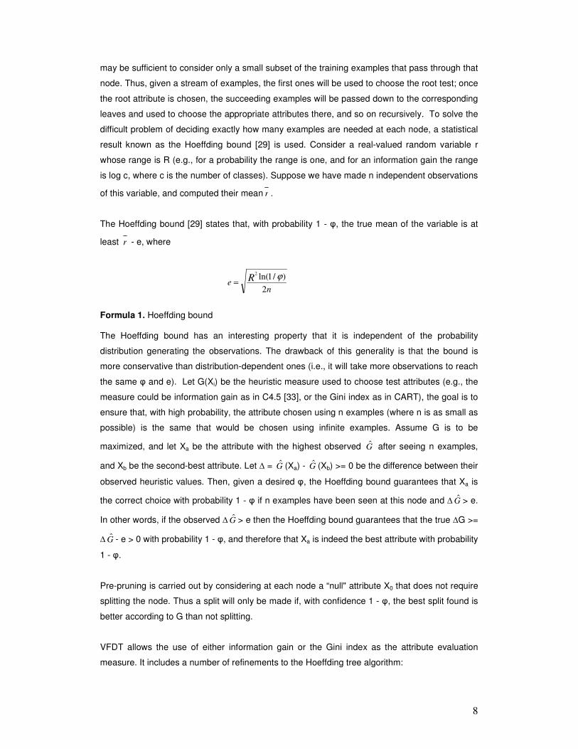
difficult problem of deciding exactly how many examples are needed at each node, a statistical

result known as the Hoeffding bound [29] is used. Consider a real-valued random variable r

whose range is R (e.g., for a probability the range is one, and for an information gain the range

is log c, where c is the number of classes). Suppose we have made n independent observations

of this variable, and computed their mean r .

The Hoeffding bound [29] states that, with probability 1 - �, the true mean of the variable is at

least r - e, where

ne

R2

)/1ln(2

ϕ=

Formula 1. Hoeffding bound The Hoeffding bound has an interesting property that it is independent of the probability

distribution generating the observations. The drawback of this generality is that the bound is

more conservative than distribution-dependent ones (i.e., it will take more observations to reach

the same � and e). Let G(Xi) be the heuristic measure used to choose test attributes (e.g., the

measure could be information gain as in C4.5 [33], or the Gini index as in CART), the goal is to

ensure that, with high probability, the attribute chosen using n examples (where n is as small as

possible) is the same that would be chosen using infinite examples. Assume G is to be

maximized, and let Xa be the attribute with the highest observed G after seeing n examples,

and Xb be the second-best attribute. Let � = G (Xa) - G (Xb) >= 0 be the difference between their

observed heuristic values. Then, given a desired �, the Hoeffding bound guarantees that Xa is

the correct choice with probability 1 - � if n examples have been seen at this node and � G > e.

In other words, if the observed � G > e then the Hoeffding bound guarantees that the true �G >=

� G - e > 0 with probability 1 - �, and therefore that Xa is indeed the best attribute with probability

1 - �.

Pre-pruning is carried out by considering at each node a “null" attribute X0 that does not require

splitting the node. Thus a split will only be made if, with confidence 1 - �, the best split found is

better according to G than not splitting.

VFDT allows the use of either information gain or the Gini index as the attribute evaluation

measure. It includes a number of refinements to the Hoeffding tree algorithm:

9

Ties: VFDT can optionally decide that there is effectively a tie and split on the current best

attribute if � G < e < t, where t is a user-specified threshold.

G computation: The most significant part of the time cost per example is re-computing G. It is

inefficient to re-compute G for every new example, because it is unlikely that the decision to

split will be made at that specific point. Thus VFDT allows the user to specify a minimum

number of new examples nmin that must be accumulated at a leaf before G is recomputed.

Memory: If the maximum available memory is ever reached, VFDT deactivates the least

promising leaves in order to make room for new ones.

Poor attributes: Memory usage is also minimized by dropping early on attributes that do not

look promising. As soon as the difference between an attribute's G and the best one's becomes

greater than e, the attribute can be dropped from consideration, and the memory used to store

the corresponding counts can be freed.

Initialization: VFDT can be initialized with the tree produced by a conventional RAM-based

learner on a small subset of the data.

Rescans: VFDT can rescan previously-seen examples. This option can be activated if either

the data arrives slowly enough that there is time for it, or if the dataset is finite and small enough

that it is feasible to scan it multiple times.

VFDT assumes that the concepts to be learned are stable over time.

Another modification on induction trees is presented in [7]. Here it is used in the form of

functional Tree Leaves. This is a hybrid algorithm that generates a regular univariate decision

tree, but the leaves contain a Naive Bayes classifier built from the examples that fall at this

node. The approach retains the interpretability of Naive Bayes and decision trees, while

resulting in classifiers that frequently outperform both constituents, especially in large datasets.

On the other hand, in [12] it is proposed using weighted classifier ensembles to mine streaming

data with concept changes. Instead of continuously revising a single model, an ensemble of

classifiers from sequential are trained from data chunks in the stream. Maintaining the most up-

to-date classifier is not necessarily the ideal choice, because potentially valuable information

may be wasted by discarding results of previously-trained less-accurate classifiers. In that work

[12], it is showed that the expiration of old data must rely on data’s distribution instead of only

their arrival time. The ensemble approach offers this capability by giving each classifier a weight

based on its expected prediction accuracy on the current test examples.

2.1 Concept Drift

A difficult problem with learning in many real-world domains is that the concept of interest may

depend on some hidden context, not given explicitly in the form of predictive features. A typical

10

example is weather prediction rules that may vary radically with the season. Another example

is the patterns of customers’ buying preferences that may change depending on products on

sale, availability of alternatives, inflation rate, etc. Often the cause of change is hidden, not

known a priori, making the learning task more complicated. Changes in the hidden context can

induce more or less radical changes in the target concept, which is generally known as concept

drift. An effective learner should be able to track such changes and quickly adapt to them.

Several authors have been working on concept drift [1, 4, 9] since it is an important

characteristic that incremental learning and data streams algorithms must deal with.

A difficult problem in handling concept drift is distinguishing between the true concept drift and

noise. Some algorithms may overreact to noise, erroneously interpreting it as concept drift,

while others may be highly robust to noise, adjusting to the changes too slowly. An ideal

learner should combine robustness with noise and sensitivity with concept drift.

In many domains, hidden contexts may be expected to recur. Recurring contexts may be due

to cyclic phenomena, such as seasons of the year or may be associated with irregular

phenomena, such as inflation rates or market mood. In such domains, in order to adapt more

quickly to concept drift, concept descriptions may be saved so that they could be reexamined

and reused later. Not many learners are able to deal with recurring contexts. Examples of

these include: FLORA3, PECS, SPLICE, Local Weights and Batch Selection. Thus, an ideal

concept drift handling system should be able to:

• Quickly adapt to concept drift.

• Be robust to noise and distinguish it from concept drift.

• Recognize and treat recurring contexts.

Two kinds of concept drifts that may occur in the real world are normally distinguished in the

literature: (1) sudden (abrupt, instantaneous), and (2) gradual concept drift. For example,

someone graduating from college might suddenly have completely different monetary concerns,

whereas a slowly wearing piece of factory equipment might cause a gradual change in the

quality of output parts. In addition, gradual drift is divided further into moderate/frequent and

slow drifts, depending on the rate of the changes.

Hidden changes in context may not only be a cause of a change of target concept, but may also

cause a change of the underlying data distribution. Even if the target concept remains the same,

and it is only the data distribution that changes, this may often lead to the necessity of revising

the current model, as the model’s error may no longer be acceptable with the new data

distribution. The necessity in the change of current model due to the change of data distribution

is called virtual concept drift.

11

2.2 Previous works We have identified a number of related works that are discussed below. For example, in [1], the

authors have designed different experiments to evaluate the STAGGER algorithm. The

experiment was focused on concept drift and noisy data. In fact, they tried to design an

algorithm that must be able to distinguish between noise and concept change. At any given

prediction failure, the questing arise as to whether this failure is simple due to noise or whether

it is indicative that the concept is beginning to drift. To do that, it was defined a domain of

objects that can be described by size = {small, medium, large}, colour = {red, blue, green},

and shape = {circle, square, triangle}. A characteristic matching any object which is both

small and red or is not a square would be represented as: (size = small and colour = red) or

shape = (circle or triangle). In addition, it was defined a sequence of 3 target concepts that

the algorithm must be able to adapt: (1) size = small and colour = red, (2) colour = green or

shape = circular, and (3) size = (medium or large). It was defined a number of randomly

training examples forced to change the concept definition at each constant number of instances.

It started with examples responding to concept definition (1). After a constant number of

instances, a concept drift was simulated so the examples started to respond to concept

definition (2). Then the same process occurred to change from concept definition (2) to concept

definition (3).

With this experiment, the authors evaluate the STAGGER algorithm in several ways. They

plotted a graph comparing correctly classified vs. concept drift. In this experiment they noticed

how performance falls immediately following the change because the previously acquired

definition was not sufficient to characterize newly changed instances. Another comparative

experiment was memory usage vs. concept drift. As a conclusion of this experiment, they

noticed that as effective characterizations are established, their sponsoring components are

pruned and the size of the search frontier is reduced. Also, they noticed how backtracking is

triggered after each concept change, resulting in a sharp climb in the size of the frontier as

previously effective characterizations are impeached. The last experiment was comparing

correctly classified examples vs. concept drift as the first one. The only difference here is that

they increased the number of training examples for each concept to four times. As a result,

they noticed that the less frequently a concept drift is produced, the quicker the algorithm could

adapt to it.

Another benchmarking analysis applied to classification algorithms that adapt to concept drift

was performed in [2]. The goal of this work is to evaluate different forgetting mechanisms.

Here the author noticed that some time-forgetting mechanisms use a function for aging the

examples and the ones that are older than a certain age are forgotten. These approaches totally

forget the observations that are outside the given window or older than certain age. The

examples, which remain in the partial memory, are equally important for the learning algorithms.

This is abrupt and total forgetting of old information, which in some cases can be valuable. To

12

avoid loss of useful knowledge learned from old examples, some systems keep old rules till they

are competitive to the new ones. The paper presents a method for gradual forgetting, that is

applied for learning drifting concepts. The approach suggests the introduction of a time-based

forgetting function, which makes the last observations more significant for the learning

algorithms than the old ones. The importance of examples decreases with time. Namely, the

forgetting function provides each training example with a weight, according to its appearance

over time. This work used the STAGGER’s experiment previously described. The classification

algorithm used was ID3. The first experiment compares the predictive accuracy of this

classification algorithm using a non-forgetting approach vs. a forgetting approach. The result

concludes that the forgetting approach outperforms the non-forgetting one after the first concept

drift. The second experiment compares the predictive accuracy of this classification algorithm

using a time window with totally forgetting approach vs. a time window with gradual forgetting

approach. The results in this research suggest that the gradual forgetting approach

outperforms the totally forgetting approach after the first concept drift. After that, the author

repeats the same experiments with the Naïve Bayes algorithm, obtaining the same results.

In [3] the author makes several comparisons to four classification algorithms. The four

algorithms involved are: RePro, WCE, DWCE and CVFT. In addition to the comparisons, the

author presents the RePro algorithm. To compare and evaluate these algorithms, three

experiments are performed: the STAGGER’s experiment previously described, Hyperplane and

Network Intrusion. Regarding the Hyperplane, it can simulate concept drift by its continuous

moving. A hyper plane in a d-dimensional space [0; 1]d is denoted by � =

=d

1i0ii w xw , where each

vector of variables < x1; … ; x d > is a randomly generated instance and is uniformly distributed.

Instances satisfying � >==

d1i

0ii w xw are labelled as positive, and otherwise negative. The value

of each coefficient wi is continuously changed so that the hyper plane is gradually drifting in the

space. Besides, the value of w0 is always set as � =d

1ii w2/1 so that roughly half of the instances

are positive, and the other half are negative. Particularly in this experiment, wi's changing range

is [-3,+3] and its changing rate is 0.005 per instance.

On the other hand, Network intrusion can simulate sampling change. It was used for the 3rd

international KDD Tools Competition [31]. It includes a wide variety of intrusions simulated in a

military network environment. The task is to build a prediction model capable of distinguishing

between normal connections (Class 1) and network intrusions (Classes 2, 3, 4, 5). Different

periods witness bursts of different intrusion classes. Assuming that all data are simultaneously

available, learners like C4.5 [33] can achieve high classification accuracy on the whole data set.

Hence one may think that there is only a single concept underlying the data. However, in the

context of streaming data, a learner's observation is limited since instances come one by one.

This study evaluates the four algorithms previously mentioned on the three experiments. The

first comparison evaluates the error rate. The results show that RePro gets the best accuracy

over STAGGER’s and Intrusion’s experiment, while DWCE gets the best accuracy over

13

Hyperplane’s experiment. The second experiment evaluates the processing time. Here it is

showed that DWCE spends more time than the other ones.

Another work was performed in [4]. Here Splice-1 and Splice-2 algorithms are presented. The

first experiment compares the accuracy of Splice-1 to C4.5 when trained on a data set

containing changes in a hidden context. The training set consisted of three concepts (labelled

1, 2 and 3) with 50 instances in each one. The test set also consisted of three concepts

(labelled 1, 2 and 3) with 50 instances in each one. This experiment is similar to the

STAGGER’s experiment. The results show that Splice-1 successfully identified the local

concepts from the training set and that the correct local concept can be successfully selected

for prediction purposes in better than 95% of cases. This experiment was made with a data set

that contained 30% noise. The second experiment analyses the effects of noise and duration

on Splice-1. To do this, the training sets were generated using a range of concept duration and

noise. Concept duration corresponds to the number of instances for which a concept is active.

That is, for some duration D, it was generated a training set containing D instances for concept

1, D instances for concept 2 and D instances for concept 3. Duration ranges from 10 instances

to 150 instances. Noise ranges from 0% to 30%. Each combination of noise level and concept

duration was repeated 100 times. The results show the accuracy of Splice-1 in correctly

identifying each target concept under varying levels of both concept duration and noise. In this

domain, Splice-1 is well behaved, with a graceful degradation of performance as noise levels

increase. Concept duration reduces the negative effect of noise. After that, the same

experiments were performed for Splice-2 obtaining similar results.

In [5] the author applies two experiments to evaluate the OLIN algorithm presented in this

research. In the first experiment a manufacturing data set is used. The data consists of a

sample of yield data recorded at a semiconductor plant. In semiconductor industry, the yield is

defined as the ratio between the number of good parts (microelectronic chips) in a completed

batch and the maximum number of parts produced, which can be obtained from the same

batch, if no chips are scraped at one of the fabrication steps. Due to high complexity and

variability of modern microelectronics industry, the yield is anything but a stationary process. In

the experiment it was assumed that the online learning starts after the completion of the first

378 batches, which leaves the algorithm with exactly 1000 records for validating the

performance of the constructed model. The experiment compares the performance of four

methods for online learning: no retraining, no-forgetting (initial size = 100), static windowing

(size = 100, increment = 50), and dynamic windowing (OLIN). The error rates of all methods are

calculated as moving averages of the past 100 validation examples. The no re-training

approach is leading in the beginning of the run, but eventually its error goes up and it becomes

inferior to other methods most of the time, probably due to changes in the yield behavior. The

no-forgetting method is consistently providing the most accurate predictions for nearly the entire

length of the data stream. The static windowing performed better than OLIN during the first 900

records in the stream. Afterwards, there is a sharp increase in the error rate of the static

14

windowing, while OLIN and the no-forgetting provide the lowest error. In other words, by the end

of the run, the large windows of OLIN and the no-forgetting method are more accurate than the

small, fixed-size windows of the static method.

The second experiment was performed on a stock market dataset. The raw data represents the

daily stock prices of 373 companies over a 5-year period (from 8/29/94 to 8/27/99). The

classification problem has been defined as predicting the correct length of the current interval

based on the known characteristics of the current and the preceding intervals. The candidate

input attributes include the duration, the slope, and the fluctuation measured in each interval, as

well as the major sector of the corresponding stock (a static attribute). The target attribute,

which is the duration of the second interval in a pair, has been categorized to five sub-intervals

of nearly equal frequency. These sub-intervals have been labelled as very short, short, medium,

etc. This dataset is non-stationary. The experiment compares the performance of the “no re-

training” approach, no-forgetting (initial size = 100, increment = 100), static windowing (size =

400, increment = 200), and dynamic windowing (OLIN). The error rates of all methods are

calculated as moving averages of the past 400 validation examples. During the first 40% of the

run, while the concept appears to be stable, no method is consistently better or consistently

worse than the other two, which is quite reasonable. In the next segment, which is characterized

by a high rate of concept drift, the static windowing approach is less successful than OLIN.

However, OLIN itself performs worse in this segment than the no-forgetting learner. At the

same time, one can see that the gap between OLIN and the no-forgetting method remains

nearly constant as more examples arrive. The “no retraining” approach is close to static

windowing most of the time, but it becomes extremely inaccurate for the last 800 examples of

the run, since it does not adjust itself to an abrupt change in the underlying concept.

2.3 Conclusion

In this section we could see that analyzing data streams generates new challenges in the data

mining process. This is mainly because a data stream is a sequence of ordered items arriving

in time domain, in some cases with no particular patterns, even arriving faster than the time

needed to be mined. In addition, and because a data stream is an infinite sequence of items,

some changes in the underlying data distribution may occur (called concept drift), requiring that

the model has to detect and adapt to these changes. These characteristics make off-line

learning algorithms not suitable for data streams. In fact, the algorithms used to mine data

streams come from the on-line or incremental learning area. Incremental learning assumes that

the items are time-ordered and the distribution that generates them varies over time. The main

challenge in incremental learning is how to detect and adapt to a concept drift. Basically, the

algorithms need to drop the data that belongs to the old concept and use the data that belongs

to the new concept. To do this, some approaches have been developed: instance selection

(basically using a fixed or dynamic window), instance weighting (dropping all the instances that

15

weight less than a threshold) and ensemble learning (using and ensemble of classification

algorithms), are a few to name. On the other hand, to deal with the problem of the data that

arrives fast, the algorithms must require a small constant processing time per record, use only a

fixed amount of main memory and must be able to build a model using at most one scan of the

data. One of the first algorithms developed for this purpose was VFDT. This algorithm uses an

interesting statistical measure (the Hoeffding bound) to determine the number of examples

needed at each tree node.

Regarding concept drift, we could see that a difficult problem is to distinguish between a true

concept drift and noise. This is because some algorithms may overreact to noise, erroneously

interpreting it as a concept drift, while others may be highly robust to noise, adjusting to the

changes too slowly. In addition, we could see that there are different types of concept drifts:

sudden concept drift, gradual concept drift, virtual concept drift and recurring concept drift are

the ones to name here.

If we focus on previous benchmarking analysis, we find the experiment used to evaluate the

STAGGER algorithm. This experiment compares how this algorithm reacts when a concept drift

is presented. Other experiment compares a totally forgetting approach and a gradually

forgetting approach while another one compares four algorithms using the Hyperplane code

generator.

Although some benchmarking analyses have been done previously, we didn’t find any

benchmarks that compare the aspects presented here using these data stream algorithms.

16

3 Description of evaluated algorithms

3.1 VFDTc algorithm

The Very Fast Decision Tree for continuous attributes (VFDTc) algorithm is presented in [7].

This algorithm is an extension to VFDT in three directions: the ability to deal with continuous

data, the use of more powerful classification techniques at tree leaves (the use of functional

leaves), and the ability to detect and react to concept drift. VFDTc system can incorporate and

classify new information online, with a single scan of the data, and in a timely fashion that is

constant per example.

In VFDTc a decision node that contains a split-test based on a continuous attribute has two

descendant branches. The split-test is a condition of the form attri <= cut_point. The descendant

branches correspond to the values TRUE and FALSE for the split-test. The cut_point is chosen

from all the possible observed values for that attribute. In order to evaluate the goodness of a

split, it needs to compute the class distributions of the examples where the attribute-value is

less than and greater than the cut_point. The counts nijk (number of examples that reached the

leaf with class k, attribute j and attribute-value i) are fundamental for computing all necessary

statistics, they are kept with the use of the following data structure: In each leaf of the decision

tree it maintains a vector of the class distribution of the examples that reach this leaf. For each

continuous attribute j, the system maintains a binary tree structure. A node in the binary tree is

identified with a value i (that is the value of the attribute j seen in an example), and two vectors,

VE and VH (of dimension k), used to count the values per class that cross that node. The

vectors VE and VH contain the counts of values respectively <= i and > i for the examples

labeled with class k where i is the value of the attribute j for every single example already seen

in this node. When an example reaches a leaf, all the binary trees are updated. Figure 1

presents the algorithm to insert a value in the binary tree. Insertion of a new value in this

structure is O(log n) for the best case and n in the worst case, where n represent the number of

distinct values for the attribute seen so far.

To obtain the Information Gain of a given attribute an exhaustive method is used to evaluate the

merit of all possible cut_points. In this case, any value observed in the examples so far can be

used as cut point. For each possible cut_point, the information of the two partitions is computed

using the following equation:

info(Aj(i)) = P(Aj <= i) * iLow(Aj(i)) + P(Aj > i) * iHigh(Aj (i))

Formula 2. Infomation Gain of a given attribute Aj

where i is the split point, Aj an attribute of the dataset, iLow(Aj(i)) the information of Aj <= i and

iHigh(Aj(i)) the information of Aj > i. So it is chosen the split point that minimizes info(Aj(i)).

17

iLow(Aj(i)) = -�K

P(K = k | Aj <= i) * log2(P(K = k | Aj <= i))

Formula 3. Infomation Gain of a given attribute when Aj <= i

iHigh(Aj(i)) = -�K

P(K = k | Aj > i) * log2(P(K = k | Aj > i))

Formula 4. Infomation Gain of a given attribute when Aj > i

Procedure InsertValueBtree(xj , y, Btree) Begin If (Btree == NULL) then

return NewNode(i = xi , VE[y]=1; y) ElseIf (xi == i) then

VE[y]++. return.

ElseIf (xj <= i) then VE[y]++. InsertValueBtree(xj , y, Btree.Left).

ElseIf (xj > i) then VH[y]++. InsertValueBtree(xj , y, Btree.Right).

End.

Fig. 1. Algorithm to insert value xj of an example label with class y into a Binary Tree. Each node of the Btree contains: i the value assigned to the node; VE vector of values less than i; VH vector of values greater than i.

These statistics are easily computed using the counts nijk, and using the algorithm presented in

Figure 2. For each attribute, it is possible to compute the merit of all possible cut_points

traversing the binary tree once. A split point for a numerical attribute is binary. The examples

would be divided into two subsets: one representing the True value of the split-test and the

other the False value of the test installed at the decision node. VFDTc only considers a possible

cut_point if and only if the number of examples in each of the subsets is higher than pmin

percentage of the total number of examples seen in the node, where pmin is a user defined

constant

Procedure LessThan(z, k, Btree) Begin if (Btree == NULL) return 0. if (i == z) return VE[k]. if (i < z) return

VE[k] + LessThan(z, k, Btree.Right). if (i > z)

return LessThan(z, k, Btree.Left). End .

Fig. 2. Algorithm to compute #(Aj <= z) for a given attribute j and class k. Functional tree leaves: To classify a test example, the example traverses the tree from the

root to a leaf. The example is classified with the most representative class of the training

examples that fall at that leaf. An innovative aspect of this algorithm is its ability to use the naive

18

Bayes classifiers at tree leaves. That is, a test example is classified with the class that

maximizes the posteriori probability given by Bayes rule assuming the independence of the

attributes given the class. There is a simple motivation for this option. VFDT only changes a leaf

to a decision node when there are sufficient numbers of examples to support the change. To

satisfy this, usually hundreds or even thousands of examples are required. To classify a test

example, the majority class strategy only uses the information about class distributions and

does not look for the attribute-values. It uses only a small part of the available information, a

crude approximation to the distribution of the examples. On the other hand, naive Bayes takes

into account not only the prior distribution of the classes, but also the conditional probabilities of

the attribute-values given the class. In this way, there is a much better exploitation of the

available information at each leaf.

Given the example e = (x1; …; xj), the class value Ck and applying Bayes theorem, it is obtained:

P(Ck | e ) = P(Ck)�P(xj | Ck).

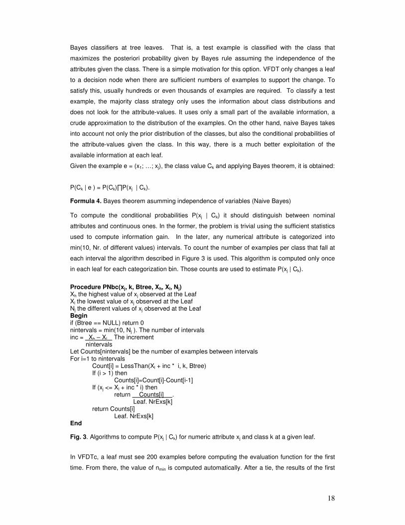
Formula 4. Bayes theorem asumming independence of variables (Naive Bayes) To compute the conditional probabilities P(xj | Ck) it should distinguish between nominal

attributes and continuous ones. In the former, the problem is trivial using the sufficient statistics

used to compute information gain. In the later, any numerical attribute is categorized into

min(10, Nr. of different values) intervals. To count the number of examples per class that fall at

each interval the algorithm described in Figure 3 is used. This algorithm is computed only once

in each leaf for each categorization bin. Those counts are used to estimate P(xj | Ck).

Procedure PNbc(xj, k, Btree, Xh, Xl, Nj) Xh the highest value of xj observed at the Leaf Xl the lowest value of xj observed at the Leaf Nj the different values of xj observed at the Leaf Begin if (Btree == NULL) return 0 nintervals = min(10, Nj ). The number of intervals inc = Xh – Xl The increment nintervals Let Counts[nintervals] be the number of examples between intervals For i=1 to nintervals

Count[i] = LessThan(Xl + inc * i, k, Btree) If (i > 1) then

Counts[i]=Count[i]-Count[i-1] If (xj <= Xl + inc * i) then

return Counts[i] . Leaf. NrExs[k]

return Counts[i] Leaf. NrExs[k]

End

Fig. 3. Algorithms to compute P(xj | Ck) for numeric attribute xj and class k at a given leaf.

In VFDTc, a leaf must see 200 examples before computing the evaluation function for the first

time. From there, the value of nmin is computed automatically. After a tie, the results of the first

19

computation, we can determine �H = H(xa) - H(xb), where H(x) is the information gain

associated with attribute x. Let NrExs be the number of examples (total) in the leaf, we can

compute the contribution, Cex, of each example to �H:

NrExs

HCex

∆=

Formula 5. Contribution of each example to �H To transform a leaf into a decision node, it must check that �H > e. If each example contributes

to Cex, then we need at least:

exC

Hen

∆−=min

Formula 6. Calculation of nmin examples to make �H > e.

When a leaf is expanded and becomes a decision node, all the sufficient statistics are released

except the statistics that deals with missing values. During this process, mean and mode for

continuous and nominal attributes are also stored.

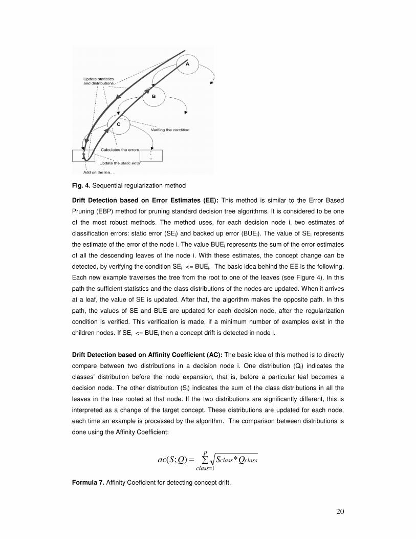
Detecting and reacting to Concept Drift: The method to detect drift is based on the

assumption that whatever is the cause of the drift, the decision surface moves. This is the base

idea behind Sequential regularization. Each time a training example is processed, the example

traverses the tree from the root to a leaf. In this path, the statistics about the class-distribution at

each node are updated. After reaching a leaf, the algorithm traverses the tree again (from the

leaf to the root in the inverse path) (Figure 4). In this path, the distribution of the nodes is

compared to the sum of the distributions of the descending leaves. If a change in these

distributions is detected, the sufficient statistics of leaves are pushed-up to the node that detects

the change and the sub-tree rooted at the node is pruned.

Based on this idea the algorithm supports two methods to estimate the class-distributions at

each node of the decision tree: one based on pessimistic estimates of the error, the other based

on the affinity coefficient. Both methods are able to continuously monitor the presence of drift.

Once drift is detected the model must be adapted to the most recent distribution.

20

Fig. 4. Sequential regularization method Drift Detection based on Error Estimates (EE): This method is similar to the Error Based

Pruning (EBP) method for pruning standard decision tree algorithms. It is considered to be one

of the most robust methods. The method uses, for each decision node i, two estimates of

classification errors: static error (SEi) and backed up error (BUEi). The value of SEi represents

the estimate of the error of the node i. The value BUEi represents the sum of the error estimates

of all the descending leaves of the node i. With these estimates, the concept change can be

detected, by verifying the condition SEi <= BUEi. The basic idea behind the EE is the following.

Each new example traverses the tree from the root to one of the leaves (see Figure 4). In this

path the sufficient statistics and the class distributions of the nodes are updated. When it arrives

at a leaf, the value of SE is updated. After that, the algorithm makes the opposite path. In this

path, the values of SE and BUE are updated for each decision node, after the regularization

condition is verified. This verification is made, if a minimum number of examples exist in the

children nodes. If SEi <= BUEi then a concept drift is detected in node i.

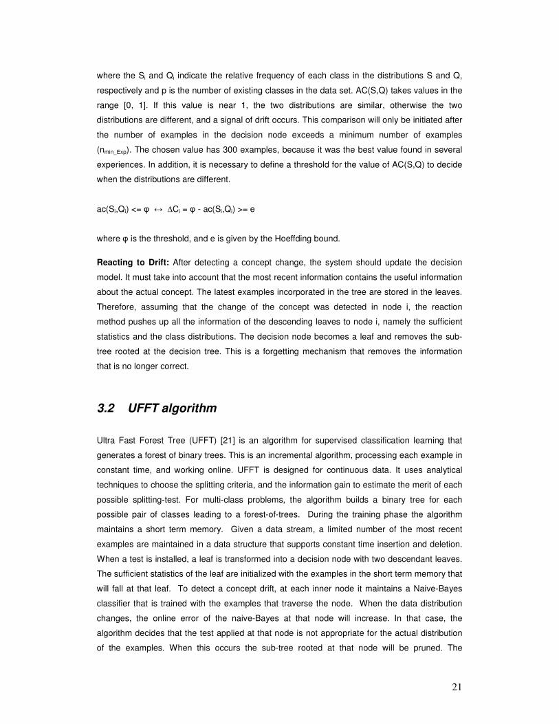
Drift Detection based on Affinity Coefficient (AC): The basic idea of this method is to directly

compare between two distributions in a decision node i. One distribution (Qi) indicates the

classes’ distribution before the node expansion, that is, before a particular leaf becomes a

decision node. The other distribution (Si) indicates the sum of the class distributions in all the

leaves in the tree rooted at that node. If the two distributions are significantly different, this is

interpreted as a change of the target concept. These distributions are updated for each node,

each time an example is processed by the algorithm. The comparison between distributions is

done using the Affinity Coefficient:

�==

p

class

classclass QSQSac1

*);(

Formula 7. Affinity Coeficient for detecting concept drift.

21

where the Si and Qi indicate the relative frequency of each class in the distributions S and Q,

respectively and p is the number of existing classes in the data set. AC(S,Q) takes values in the

range [0, 1]. If this value is near 1, the two distributions are similar, otherwise the two

distributions are different, and a signal of drift occurs. This comparison will only be initiated after

the number of examples in the decision node exceeds a minimum number of examples

(nmin_Exp). The chosen value has 300 examples, because it was the best value found in several

experiences. In addition, it is necessary to define a threshold for the value of AC(S,Q) to decide

when the distributions are different.

ac(Si,Qi) <= � � �Ci = � - ac(Si,Qi) >= e

where � is the threshold, and e is given by the Hoeffding bound.

Reacting to Drift: After detecting a concept change, the system should update the decision

model. It must take into account that the most recent information contains the useful information

about the actual concept. The latest examples incorporated in the tree are stored in the leaves.

Therefore, assuming that the change of the concept was detected in node i, the reaction

method pushes up all the information of the descending leaves to node i, namely the sufficient

statistics and the class distributions. The decision node becomes a leaf and removes the sub-

tree rooted at the decision tree. This is a forgetting mechanism that removes the information

that is no longer correct.

3.2 UFFT algorithm

Ultra Fast Forest Tree (UFFT) [21] is an algorithm for supervised classification learning that

generates a forest of binary trees. This is an incremental algorithm, processing each example in

constant time, and working online. UFFT is designed for continuous data. It uses analytical

techniques to choose the splitting criteria, and the information gain to estimate the merit of each

possible splitting-test. For multi-class problems, the algorithm builds a binary tree for each

possible pair of classes leading to a forest-of-trees. During the training phase the algorithm

maintains a short term memory. Given a data stream, a limited number of the most recent

examples are maintained in a data structure that supports constant time insertion and deletion.

When a test is installed, a leaf is transformed into a decision node with two descendant leaves.

The sufficient statistics of the leaf are initialized with the examples in the short term memory that

will fall at that leaf. To detect a concept drift, at each inner node it maintains a Naive-Bayes

classifier that is trained with the examples that traverse the node. When the data distribution

changes, the online error of the naive-Bayes at that node will increase. In that case, the

algorithm decides that the test applied at that node is not appropriate for the actual distribution

of the examples. When this occurs the sub-tree rooted at that node will be pruned. The

22

algorithm forgets the sufficient statistics and learns the new concept with only the examples in

the new concept. The drift detection method will always check the stability of the distribution

function of the examples at each decision node.

The UFFT starts with a single leaf. When a splitting test is installed at a leaf, the leaf becomes

a decision node, and two descendant leaves are generated. The splitting test has two possible

outcomes each leading to a different leaf. The value True is associated with one branch and

the value False, with the other. The splitting tests are over a numerical attribute and are of the

form attributej � valuej. For the split point selection it uses the analytical method where, for all

the numerical attributes, the most promising valuej is chosen. The only sufficient statistics

required are the mean and variance per class of each numerical attribute. The analytical

method uses a modified form of quadratic discriminant analysis to include different variances on

the two classes. This analysis assumes that the distribution of the values of an attribute follows

a normal distribution for both classes. Let N(µ, �) be the normal density function, where µ and

�2 are the mean and variance of the class. The quadratic discriminant splits the X-axis into three

intervals (−�, d1), (d1, d2), (d2,�) where d1 and d2 are the possible roots of the equation

p(−)N{(µ−, �−)} = p(+)N{(µ+, �+)}, and p(i) denotes the estimated probability that an example

belongs to class i. So the equation looks for values for which the distribution between the 2

classes (+ and -) are equal. As this algorithm uses a binary split, it uses the root closer to the

sample means of both classes. Let d be that root. The splitting test candidate for each numeric

attribute i will be of the form Atti � di. It uses the information gain to choose, from all the splitting

point candidates, the best splitting test. To compute the information gain one needs to construct

a contingency table with the distribution per class of the number of examples less than and

greater than di:

The splitting test with the maximum information gain is chosen. This method only requires that

we maintain the mean and standard deviation for each class per attribute. Both quantities are

easily maintained incrementally.

To expand a leaf node, two conditions must be satisfied. The first one requires the information

gain of the selected splitting test to be positive. That is, there is a gain in expanding the leaf

versus not expanding. The second condition is that there should exist statistical support in favor

of the best splitting test which is asserted using the Hoeffding bound as in VFDT. When new

nodes are created, the short term memory is used to update the statistics of these new leaves.

The functional leaves used by the algorithm are in charge of classifying unlabeled examples.

Each leaf uses a Naïve-Bayes classifier. In addition, it maintains sufficient statistics to compute

Atti � di Atti > di

Class + P1 + p2 +

Class - P1 - p2 -

23

the information gain and the conditional probabilities of P(xi | Class) assuming that the attribute

values follow, for each class, a normal distribution.

The splitting criterion only applies to two class problems. However, most real-world problems

are multi-class. To resolve this limitation, UFFT uses the round-robin classification technique

that decomposes a multi-class problem into k binary problems. That is, each pair of classes

defines a two-class problem. For example, in a three class problem (A, B and C) the algorithm

grows a forest of binary trees, one for each pair: A-B, B-C and A-C. In the general case of n

classes, the algorithm grows a forest of n(n-1)/2 binary trees. When a new example is received

during the training phase, each tree will receive the example if the class attached to it is one of

the two classes in the tree label. Each example is used to train several trees and none of the

trees will get all examples. The short term memory is common to all trees in the forest. When a

leaf in a particular tree becomes a decision node, only the examples corresponding to this tree

are used to initialize the new leaves.

When a new example is received during the testing phase, the algorithm sends the example to

all trees in the forest. The example will traverse the tree from the root to the leaf and the

classification will be registered. Each tree in the forest makes a prediction. This prediction takes

the form of a probability class distribution. The most probable class is used to classify the

example.

Concept drift detection: When a new training example becomes available, it will cross the

corresponding binary decision tree from the root node to the leaf. At each node, the Naïve-

Bayes installed at that node classifies the example. The example may or may not be correctly

classified. Given a set of examples, the error is a random variable from Bernoulli trials. The

Binomial distribution gives the general form of the probability for the random variable that

represents the number of errors in a sample of n examples. It is used the following estimator for

the true error of the classification function pi � (errori / i) where i is the number of examples and

errori is the number of examples misclassified, both measured in the actual context. The

standard deviation for a Binomial is given by si � )1(** pipii − , where i is the number of

examples observed within this context. For sufficient examples, the Binomial distribution is

closely approximated by a Normal distribution with the same mean and variance. Considering

that the probability distribution is unchanged when the context is static, then the 1 − �/2

confidence interval for p with n > 30 examples is approximately pi ± zn* si. The value � depends

on the confidence level. The drift detection method manages two registers during the training of

the learning algorithm: pmin and smin. Every time a new example i is processed, those values are

updated when pi + si is lower than pmin + smin. The algorithm uses a warning level to define the

optimal size of the context window. The context window will contain the old examples that are

on the new context and a minimal number of examples on the old context. Suppose that in the

sequence of examples that traverse a node, there is an example i with correspondent pi and si.

24

The warning level is reached if pi + si � pmin + 1.5 * smin. The drift level is reached if pi + si � pmin

+ 3 * smin. Consider a sequence of examples where the Naive-Bayes error increases reaching

the warning level at example kw, and the drift level at example kd. This is an indicator of a

change in the distribution of the examples. A new context is declared starting in example kw,

and the node is pruned becoming a leaf. The sufficient statistics of the leaf are initialized with

the examples in the short term memory whose time stamp is greater than kw. It is possible to

observe an increase of the error reaching the warning level, followed by a decrease. It is

assumed that such situations correspond to a false alarm, without changing the context.

3.3 CVFDT algorithm

In [22] the Concept-adapting Very Fast Decision Tree (CVFDT) algorithm is presented. This

algorithm is an extension to VFDT, previously described on section 2. CVFDT maintains

VFDT’s speed and accuracy advantages but adds the ability to detect and respond to changes.

It works by keeping its model consistent with a sliding window of examples. However, it does

not need to learn a new model from start, every time a new example arrives; instead it updates

the sufficient statistics at its nodes by incrementing the counts corresponding to the new

example, and decrementing the counts corresponding to the oldest example in the window.

In case the concept changes, CVFDT begins to grow an alternative sub-tree with the new best

attribute at its root. When this alternate sub-tree becomes more accurate on new data than the

old one, the old sub-tree is replaced by the new one. In figure 5 we can see a pseudo-code of

the CVFDT algorithm.

25

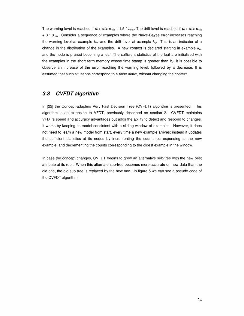
Input: S: a sequence of examples X: a set of symbolic attributes G(.): a split evaluation function

�: one minus the desired probability of choosing the correct attribute at any given node (see Hoeffding bound on section 2) t: a user-supplied tie threshold w: the size of the window nmin: count of examples between checks for growth f: count of examples between checks for drift

Output: HT: a decision tree /* initialize */ Let HT be a tree with a single leaf l1 (the root) Let ALT(l1) be an initially empty set of alternate trees for l1

Let 1G (X0) be the G obtained by predicting the most frequent class in S

Let X1 = X U { X0} Let W be the window of examples, initially empty For each class yk For each value xij of each attribute Xi � X

Let nijk(l1) = 0 /* process the examples */ For each example (x, y) in S

Sort(x, y) into a set of leaves L using HT and all trees in ALT of any node (x, y) passes through Let ID be the maximum id of the leaves in L Add ((x, y), ID) to the beginning of W If |W| > w Let ((xw, yw), IDw) be the last element of W ForgetExamples(HT, n, (xw, yw), IDw) Let W = W with ((xw, yw), IDw) removed CVFDTGrow(HT, n, G, (x, y), �, nmin, t) If there have been f examples since the last checking of alternative trees CheckSplitValidity(HT, n, �)

Return HT

Fig. 5: Pseudo code for the CVFDT algorithm. In this pseudo-code we can see that CVFDT performs some initialization, and then processes

the examples obtained from the stream S indefinitely. As each example (x, y) arrives, it is

added to the window and incorporated into the current model. At the same time and if it is

needed, an old example is forgotten. CVFDT periodically scans HT and all alternate trees

looking for internal nodes whose sufficient statistics indicate that some new attribute would

make a better test than the chosen split attribute. An alternate sub-tree is started at each such

node.

In figure 6 we can see a pseudo-code for the tree-growing portion of the CVFDT system.

26

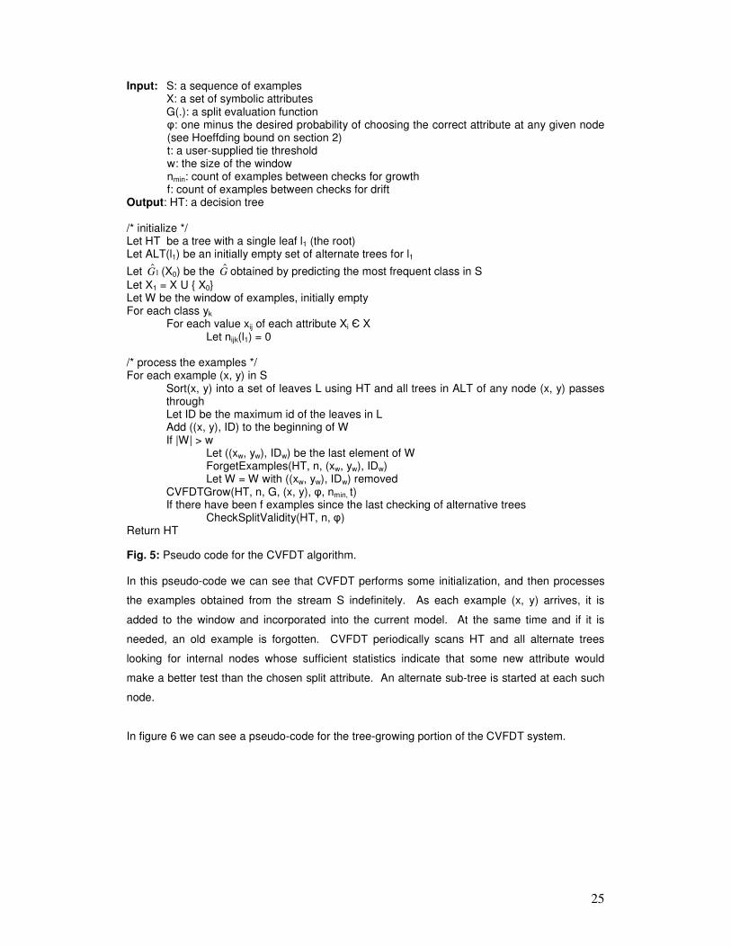
Procedure CVFDTGrow(HT, n, G, (x, y), �, nmin, t) Sort(x, y) into a leaf l using HT Let P be the set of nodes traversed in the sort For each node lpi in P For each xij in x such that Xi � Xlp

Increment nijk(lp) For each tree Ta in ALT(lp) CVFDTGrow(Ta, n, G, (x, y), �, nmin, t) Label l with the majority class among the examples seen so far at l Let nl be the number of examples seen at l. If the examples seen so far at l are not all of the same class and nl mod nmin is 0, then

Compute lG (Xi) for each attribute Xi � Xl – {X0} using the counts nijk(l)

Let Xa be the attribute with highest lG

Let Xb be the attribute with second-highest lG

Compute e using the Hoeffding bound explained on section 2 and �

Let � lG = lG (Xa) - lG (Xb)

If ((� lG > e) or (� lG <= e < t)) and Xa <> X0, then

Replace l by an internal node that splits on Xa For each branch of the split Add a new leaf lm, and let Xm = X – { Xa} Let ALT(lm) = {}

Let mG (X0) be the lG obtained b predicting the most frequent class at lm

For each class yk and each value xij of each attribute Xi � Xm – {X0} Let nijk(lm) = 0

Fig. 6: The CVFDTGrow procedure This procedure is similar to the Hoeffding Tree algorithm, but CVFDT monitors the validity of its

old decisions by maintaining sufficient statistics at every node in HT. Forgetting an old example

is slightly complicated due to the fact that HT may have grown or changed since the example

was initially incorporated. Therefore, nodes are assigned a unique, monotonically increasing ID

as they are created. When an example is added to W, the maximum ID of the leaves it reaches

in HT and all alternate trees is recorded with it. An example’s effect is forgotten by

decrementing the counts in the sufficient statistics of every node the example reaches in HT

whose ID is <= the stored ID. The forgetting procedure pseudo-code is detailed on figure 7.

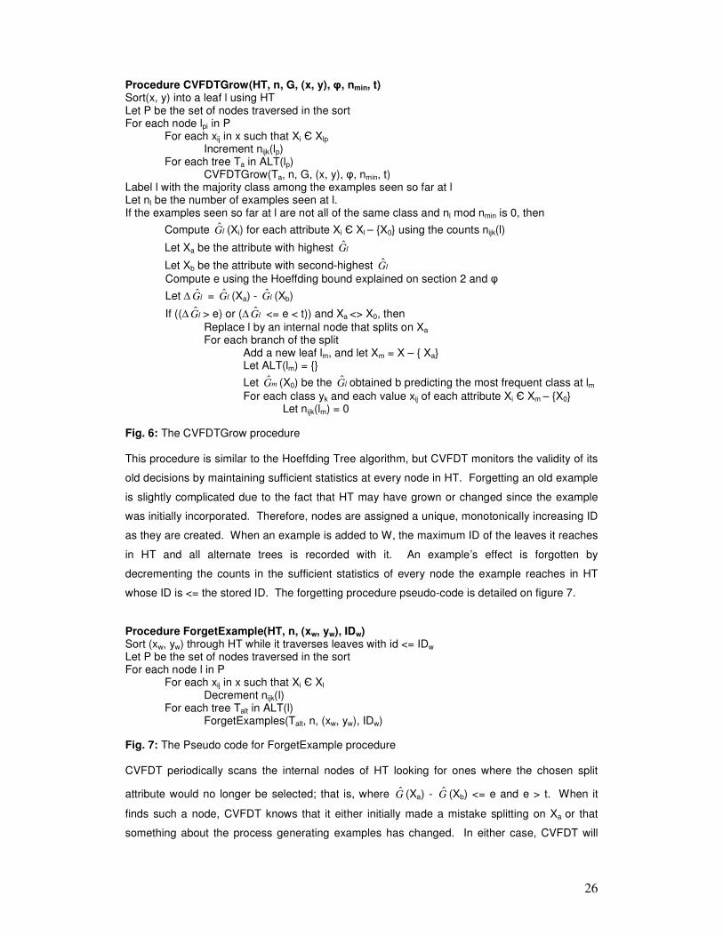
Procedure ForgetExample(HT, n, (xw, yw), IDw) Sort (xw, yw) through HT while it traverses leaves with id <= IDw Let P be the set of nodes traversed in the sort For each node l in P For each xij in x such that Xi � Xl Decrement nijk(l) For each tree Talt in ALT(l) ForgetExamples(Talt, n, (xw, yw), IDw)

Fig. 7: The Pseudo code for ForgetExample procedure CVFDT periodically scans the internal nodes of HT looking for ones where the chosen split

attribute would no longer be selected; that is, where G (Xa) - G (Xb) <= e and e > t. When it

finds such a node, CVFDT knows that it either initially made a mistake splitting on Xa or that

something about the process generating examples has changed. In either case, CVFDT will

27

need to take action to correct HT. CVFDT grows alternate sub-trees, and only modifies HT

when the alternate is more accurate than the original.

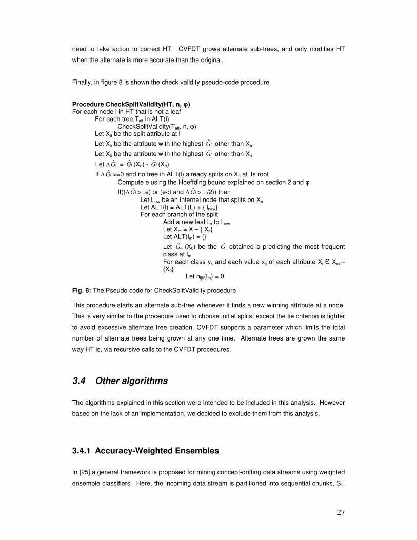
Finally, in figure 8 is shown the check validity pseudo-code procedure.

Procedure CheckSplitValidity(HT, n, �) For each node l in HT that is not a leaf For each tree Talt in ALT(l) CheckSplitValidity(Talt, n, �) Let Xa be the split attribute at l

Let Xn be the attribute with the highest lG other than Xa

Let Xb be the attribute with the highest lG other than Xn

Let � lG = lG (Xn) - lG (Xb)

If � lG >=0 and no tree in ALT(l) already splits on Xn at its root

Compute e using the Hoeffding bound explained on section 2 and �

If((� lG >=e) or (e<t and � lG >=t/2)) then

Let lnew be an internal node that splits on Xn Let ALT(l) = ALT(L) + { lnew} For each branch of the split Add a new leaf lm to lnew Let Xm = X – { Xn}

Let ALT(lm) = {}

Let mG (X0) be the G obtained b predicting the most frequent

class at lm For each class yk and each value xij of each attribute Xi � Xm – {X0}

Let nijk(lm) = 0

Fig. 8: The Pseudo code for CheckSplitValidity procedure This procedure starts an alternate sub-tree whenever it finds a new winning attribute at a node.

This is very similar to the procedure used to choose initial splits, except the tie criterion is tighter

to avoid excessive alternate tree creation. CVFDT supports a parameter which limits the total

number of alternate trees being grown at any one time. Alternate trees are grown the same

way HT is, via recursive calls to the CVFDT procedures.

3.4 Other algorithms

The algorithms explained in this section were intended to be included in this analysis. However

based on the lack of an implementation, we decided to exclude them from this analysis.

3.4.1 Accuracy-Weighted Ensembles

In [25] a general framework is proposed for mining concept-drifting data streams using weighted

ensemble classifiers. Here, the incoming data stream is partitioned into sequential chunks, S1,

28

S2, …, Sn, with Sn being the most up-to-date chunk, and each chunk is of the same size, or

ChunkSize. A classifier Ci is learned for each Si, i >= 1. According to the error reduction

property, given test examples T, each classifier Ci should be assigned a weight reversely

proportional to the expected error of Ci in classifying T. To do this, it is necessary to know the

actual function being learned, which is unavailable. Thus, the weight of classifier Ci is derived

by estimating its expected prediction error on the test examples. It is assumed that the class

distribution of Sn, the most recent training data, is closest to the class distribution of the current

test data. Thus, the weights of the classifiers can be approximated by computing their

classification error on Sn. More specifically, assume that Sn consists of records in the form of

(x,c), where c is the true label of the record. Ci’s classification error of example (x,c) is )(1 xfi

c− ,

where )( xfi

c is the probability given by Ci that x is an instance of class c. Thus, the mean

square error of classifier Ci can be expressed by:

� −=Sncxn

xf icS

MSE i

ε),(

2

))(1(||

1

Formula 8. Mean square error of classifier Ci.

The weight of classifier Ci should be reversely proportional to MSEi. On the other hand, what a

classifier randomly predicts (that is, the probability of x being classified as class c equals to c’s

class distributions p(c)) will have a mean square error of:

� −=c

r cpcpMSE ))(1)((2

Formula 9. Mean square error of a random model. For instance, if c � {0, 1} and the class distribution is uniform, we have MSEr = 0.25. Since a

random model does not contain useful knowledge about the data, the error rate of the random

classifier, MSEr, is used as a threshold in weighting the classifiers. In other words, it is

discarded classifiers whose error is equal to or larger than MSEr. Furthermore, to make

computation easy, the following weight wi is used for classifier Ci:

iri MSEMSEw −=

For cost-sensitive applications such as credit card fraud detection, the benefits (e.g., total fraud

amount detected) achieved by classifier Ci are used on the most recent training data Sn as its

weight.

Since the algorithm handles infinite incoming data flows, it will learn an infinite number of

classifiers over time. It is impossible and unnecessary to keep and use all the classifiers for

prediction. Instead, it only keeps the top K classifiers with the highest prediction accuracy on

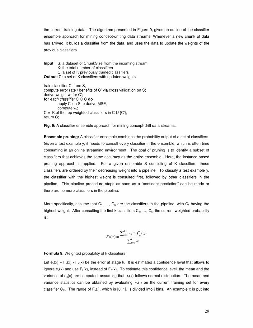
29

the current training data. The algorithm presented in Figure 9, gives an outline of the classifier

ensemble approach for mining concept-drifting data streams. Whenever a new chunk of data

has arrived, it builds a classifier from the data, and uses the data to update the weights of the

previous classifiers.

Input: S: a dataset of ChunkSize from the incoming stream K: the total number of classifiers C: a set of K previously trained classifiers

Output: C: a set of K classifiers with updated weights train classifier C’ from S; compute error rate / benefits of C’ via cross validation on S; derive weight w’ for C’; for each classifier Ci � C do

apply Ci on S to derive MSEi; compute wi;

C = K of the top weighted classifiers in C U {C’}; return C;

Fig. 9: A classifier ensemble approach for mining concept-drift data streams.

Ensemble pruning: A classifier ensemble combines the probability output of a set of classifiers.

Given a test example y, it needs to consult every classifier in the ensemble, which is often time

consuming in an online streaming environment. The goal of pruning is to identify a subset of

classifiers that achieves the same accuracy as the entire ensemble. Here, the instance-based

pruning approach is applied. For a given ensemble S consisting of K classifiers, these

classifiers are ordered by their decreasing weight into a pipeline. To classify a test example y,

the classifier with the highest weight is consulted first, followed by other classifiers in the

pipeline. This pipeline procedure stops as soon as a “confident prediction” can be made or

there are no more classifiers in the pipeline.

More specifically, assume that C1, …, CK are the classifiers in the pipeline, with C1 having the

highest weight. After consulting the first k classifiers C1, …, Ck, the current weighted probability

is:

�

�

=

==

k

ii

k

i

i

ci

k

w

xwxF

f

1

1 )(*)(

Formula 9. Weighted probability of k classifiers. Let ek(x) = Fk(x) - FK(x) be the error at stage k. It is estimated a confidence level that allows to

ignore ek(x) and use Fk(x), instead of FK(x). To estimate this confidence level, the mean and the

variance of ek(x) are computed, assuming that ek(x) follows normal distribution. The mean and

variance statistics can be obtained by evaluating Fk(.) on the current training set for every

classifier CK. The range of Fk(.), which is [0, 1], is divided into j bins. An example x is put into

30

bin i if Fk(x) � [j

i ,j

i 1+ ). Then we compute µ k,i and σ2k,i, which are the mean and the variance

of the error of those training examples in bin i at stage k. Finally, to classify a new instance y,

the following decision rules are applied for each classifier in the pipeline:

Fk(y) - µ k,i - t * σ2k,i > threshold, C class

Fk(y) + µ k,i + t * σ2k,i <= threshold, ¬C class

Otherwise, uncertain

where i is the bin that y belongs to, and t is a confidence interval parameter. Assuming that we

have a normal distribution, t = 3 delivers a confidence of 99.7%, and t = 2 of confidence 95%.

When the prediction is uncertain, that is, the instance falls out of the t sigma region, the next

classifier in the pipeline, Ck+1, is employed and the rules are applied again. If there are no

classifiers left in the pipeline, the current prediction is returned. As a result, an example does

not need to use all classifiers in the pipeline to compute a prediction with high confidence. The

“expected” number of classifiers can be reduced. Figure 10 details the classifier ensemble

approach previously described in Figure 5 with the addition of the mean and the variance of

ek(x) calculation.

Input: S: a dataset of ChunkSize from the incoming stream K: the total number of classifiers J: number of bins C: a set of K previously trained classifiers

Output: C: a set of K classifiers with updated weights

µ , σ : mean and variance for each stage and each bin

train classifier C’ from S; compute error rate / benefits of C’ via cross validation on S; derive weight w’ for C’; for each classifier Ci � C do

apply Ci on S to derive MSEi; compute wi;

C = K of the top weighted classifiers in C U {C’}; for each y � S do

compute Fk(y) for k = 1, …, K;

y belongs to bin (i, k) if Fk(y) � [j

i ,j

i 1+ );

incrementally updates µ k,i and σ k,i for bin (i; k);

Fig. 10: Obtaining µ k,i and σ k,i during ensemble construction.

Finally, in figure 11 it is detailed the instance based pruning algorithm previously described.

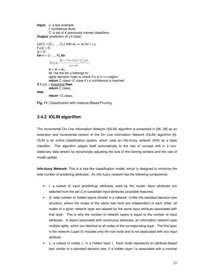
31

Input: y: a test example t: confidence level C: a set of K previously trained classifiers

Output: prediction of y’s class Let C = {C1, …, Cn} with wi >= wj for i < j; F0(y) = 0; w = 0; for k = {1 …, K} do

k

i

kkk

k

ww

xfwwFyF

+

+=

− )(**)(

1;

w = w + wk; let i be the bin y belongs to; apply decision rules to check if y is in t-� region; return C class/¬C class if t-� confidence is reached;

if FK(y) > threshold then return C class;

else return ¬C class;

Fig. 11: Classification with Instance Based Pruning.

3.4.2 IOLIN algorithm

The Incremental On Line Information Network (IOLIN) algorithm is presented in [26, 28] as an

extension and incremental version of the On Line Information Network (OLIN) algorithm [5].

OLIN is an online classification system, which uses an info-fuzzy network (IFN) as a base

classifier. This algorithm adapts itself automatically to the rate of concept drift in a non-

stationary data stream by dynamically adjusting the size of the training window and the rate of

model update.

Info-fuzzy Network: This is a tree-like classification model, which is designed to minimize the

total number of predicting attributes. An info-fuzzy network has the following components:

• I: a subset of input (predicting) attributes used by the model. Input attributes are

selected from the set C of candidate input attributes (available features).

• |I|: total number of hidden layers (levels) in a network. Unlike the standard decision tree

structure, where the nodes of the same tree level are independent of each other, all

nodes of a given network layer are labeled by the same input attribute associated with

that layer. This is why the number of network layers is equal to the number of input

attributes. In layers associated with continuous attributes, an information network uses

multiple splits, which are identical at all nodes of the corresponding layer. The first layer

in the network (Layer 0) includes only the root node and is not associated with any input

attribute.

• Ll: a subset of nodes z in a hidden layer l. Each node represents an attribute-based

test, similar to a standard decision tree. If a hidden layer l is associated with a nominal

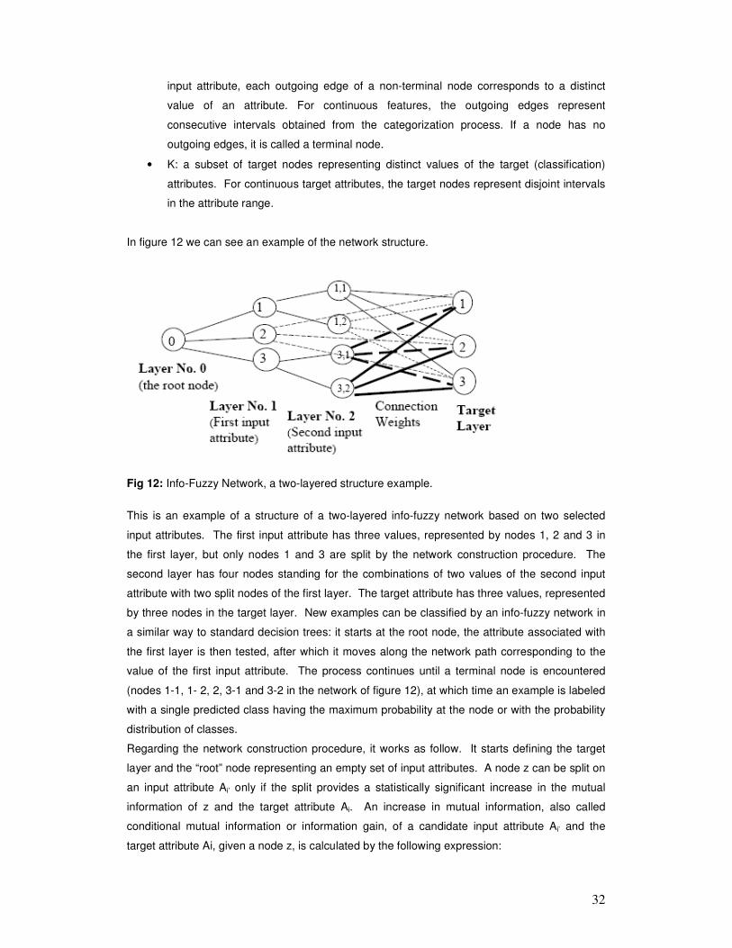
32

input attribute, each outgoing edge of a non-terminal node corresponds to a distinct

value of an attribute. For continuous features, the outgoing edges represent

consecutive intervals obtained from the categorization process. If a node has no

outgoing edges, it is called a terminal node.

• K: a subset of target nodes representing distinct values of the target (classification)

attributes. For continuous target attributes, the target nodes represent disjoint intervals

in the attribute range.

In figure 12 we can see an example of the network structure.

Fig 12: Info-Fuzzy Network, a two-layered structure example.

This is an example of a structure of a two-layered info-fuzzy network based on two selected

input attributes. The first input attribute has three values, represented by nodes 1, 2 and 3 in

the first layer, but only nodes 1 and 3 are split by the network construction procedure. The

second layer has four nodes standing for the combinations of two values of the second input

attribute with two split nodes of the first layer. The target attribute has three values, represented

by three nodes in the target layer. New examples can be classified by an info-fuzzy network in

a similar way to standard decision trees: it starts at the root node, the attribute associated with

the first layer is then tested, after which it moves along the network path corresponding to the

value of the first input attribute. The process continues until a terminal node is encountered

(nodes 1-1, 1- 2, 2, 3-1 and 3-2 in the network of figure 12), at which time an example is labeled

with a single predicted class having the maximum probability at the node or with the probability

distribution of classes.

Regarding the network construction procedure, it works as follow. It starts defining the target

layer and the “root” node representing an empty set of input attributes. A node z can be split on

an input attribute Ai’ only if the split provides a statistically significant increase in the mutual

information of z and the target attribute Ai. An increase in mutual information, also called

conditional mutual information or information gain, of a candidate input attribute Ai’ and the

target attribute Ai, given a node z, is calculated by the following expression:

33

� �−

=

−

=

=1

0

1'

0' ''

''''

)/(*)/(

)/(log*);;()|;(

Mi

j

Mi

j ijji

jiij

jiijii

zVPzVP

zVPzVVPzAAMI

Formula 10. Mutual information for building a info-fuzzy network. Where:

• Mi / Mi’: number of distinct values of the target attribute i /candidate input attribute i’.

• P (Vi’j’/ z): an estimated conditional (a posteriori) probability of a value j’ of a candidate

input attribute i’ given a node z.

• P (Vij/ z): an estimated conditional (a posteriori) probability of a value j of the target

attribute i given a node z.

• P (Vi’j’ij/ z): an estimated conditional (a posteriori) probability of a value j’ of a candidate

input attribute i’ and a value j of the target attribute i given a node z.

• P (Vij; Vi’j’; z): an estimated joint probability of a value j of the target attribute i, a value j’

of a candidate input attribute i’ and a node z.

Conditional mutual information measures the benefit of adding an input attribute to the

information network. If the input and the target attributes are conditionally independent given a

node z, their conditional joint probability should be equal to the product of their individual

conditional probabilities. This makes the logarithmic terms in MI equation equal to zero. On the

other hand, if the knowledge of an input value either increases, or decreases the conditional

probability of a target value, the corresponding summation term becomes either positive, or

negative, respectively.

In order to evaluate the statistical significance of the estimated conditional mutual information,

the algorithm uses the likelihood-ratio as follows:

)|;(*)(*)2(ln*2)|;( ''2 zAAMIzNzAAG iiii =

Formula 11. Likelihood-ratio for evaluating the statistical significance of the estimated mutual information. Where N(z) is the number of records associated with the node z.

The Likelihood-Ratio Test is a general-purpose method for testing the null hypothesis H0 that

two discrete random variables are statistically independent. In MI equation, independence of

two attributes implies that their expected mutual information is zero. If H0 holds, then the

likelihood-ratio test statistic G2(Ai’; Ai | z) is distributed as chi-square with (NIi’(z) -1)*( NTi(z) -1)

degrees of freedom, where NIi’(z) is the number of values of a candidate input attribute i’ at

node z and NTi(z) is the number of values of the target attribute i at node z. Thus, MI(Ai’; Ai | z)

is considered statistically significant if H0 can be rejected at the significance level �:

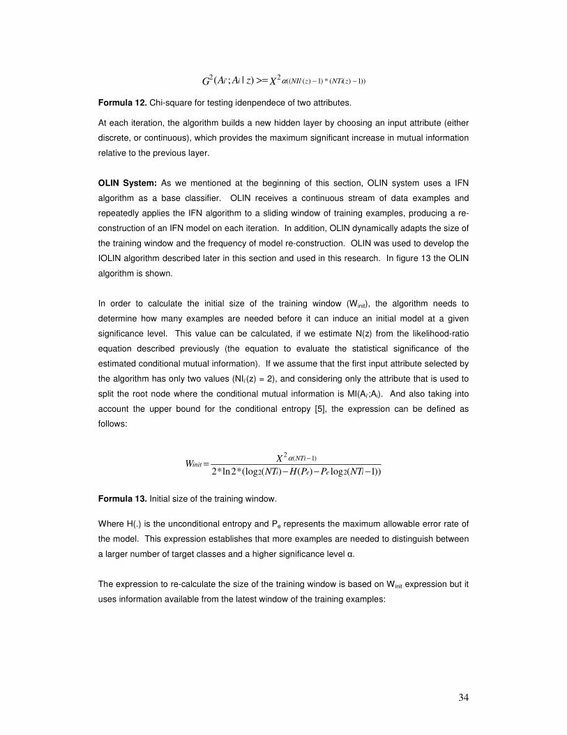
34

))1)((*)1)('((2

'2 )|;( −−>= zNTizNIiii XzAAG α

Formula 12. Chi-square for testing idenpendece of two attributes. At each iteration, the algorithm builds a new hidden layer by choosing an input attribute (either

discrete, or continuous), which provides the maximum significant increase in mutual information

relative to the previous layer.

OLIN System: As we mentioned at the beginning of this section, OLIN system uses a IFN

algorithm as a base classifier. OLIN receives a continuous stream of data examples and

repeatedly applies the IFN algorithm to a sliding window of training examples, producing a re-

construction of an IFN model on each iteration. In addition, OLIN dynamically adapts the size of

the training window and the frequency of model re-construction. OLIN was used to develop the

IOLIN algorithm described later in this section and used in this research. In figure 13 the OLIN

algorithm is shown.

In order to calculate the initial size of the training window (W init), the algorithm needs to

determine how many examples are needed before it can induce an initial model at a given

significance level. This value can be calculated, if we estimate N(z) from the likelihood-ratio

equation described previously (the equation to evaluate the statistical significance of the

estimated conditional mutual information). If we assume that the first input attribute selected by

the algorithm has only two values (NIi’(z) = 2), and considering only the attribute that is used to

split the root node where the conditional mutual information is MI(Ai’;Ai). And also taking into

account the upper bound for the conditional entropy [5], the expression can be defined as

follows:

))1(log)()((log*2ln*2 22

)1(2

−−−=

−

ieei

NTiinit

NTPPHNT

XW

α

Formula 13. Initial size of the training window.

Where H(.) is the unconditional entropy and Pe represents the maximum allowable error rate of

the model. This expression establishes that more examples are needed to distinguish between

a larger number of target classes and a higher significance level �.

The expression to re-calculate the size of the training window is based on Winit expression but it

uses information available from the latest window of the training examples:

35

))1(log)()((*2ln*2 2

)1)(1'(2

−−−=

−−

itrtri

NTiNIi

NTEEHAH

XW

α

Formula 14. Calculation of the size of the training window.

Input: S: a continuous stream of examples nmin: the number of the first example to be classified by the system (nmin – 1 examples have already arrived) nmax: the number of the last example to be classified by the system (if unspecified, the system will run indefinitely) C: a set of candidate input attributes Sign: a user-specified significance level Pe: maximum allowable prediction error of the model Init_Add_Count: the number of new examples to be classified by the first model Inc_Add_Count: amount (percentage) to increase the number of examples between model re-constructions Max_Add_Count: maximum number of examples between model re-constructions Red_Add_Count: amount (percentage) to reduce the number of examples between model reconstructions Min_Add_Count: minimum number of examples between model re-constructions Max_Win: maximum number of examples in a training window

Output: IFN: Info-fuzzy network Begin Calculate the initial size of the training window Winit (using equation described later) Let the training window size W = Winit Initialize the index i of the first training example to nmin - W Initialize the index j of the last training example to W Initialize the number of validation examples Add_Count to Init_Add_Count While j < nmax Do

Obtain a model (IFN) by applying the IN algorithm to W latest training examples Calculate the training error rate Etr of the obtained model on W training examples Calculate the index of the last validation example k = j + Add_Count Calculate the validation error rate EVal of the obtained model on Add_Count validation examples Update the index of the last training example j = k Find the maximum difference between the training and the validation errors Max_Diff (using equation described later) If (EVal - Etr) < Max_Diff // concept is stable

Add_Count =Min( Add_Count * (1+(Inc_Add_Count/100)), Max_Add_Count) W = Min (W + Add_Count, Max_Win)

Else //concept drift detected Re-calculate the size of the training window W (using equation described later) Update the index of the first training record i = j - W Add_Count = Max (Add_Count * (1-(Red_Add_Count/100)), Min_Add_Count)

Return the current model (IFN) End Do End

Fig. 13: The OLIN algorithm

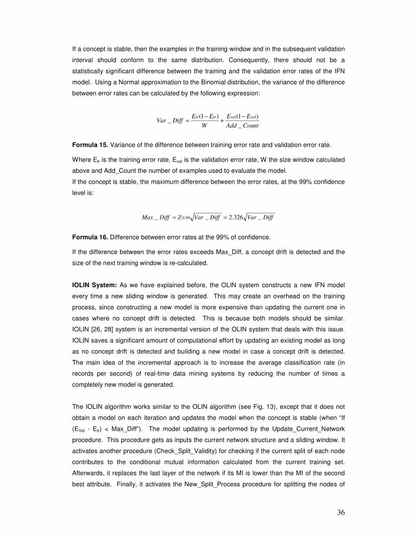
36

If a concept is stable, then the examples in the training window and in the subsequent validation

interval should conform to the same distribution. Consequently, there should not be a

statistically significant difference between the training and the validation error rates of the IFN

model. Using a Normal approximation to the Binomial distribution, the variance of the difference

between error rates can be calculated by the following expression:

CountAdd

EE

W

EEDiffVar

valvaltrtr

_

)1()1(_

−+

−=

Formula 15. Variance of the difference between training error rate and validation error rate. Where Etr is the training error rate, Eval is the validation error rate, W the size window calculated

above and Add_Count the number of examples used to evaluate the model.

If the concept is stable, the maximum difference between the error rates, at the 99% confidence

level is:

DiffVarDiffVarZDiffMax _326.2__ 99.0 ==

Formula 16. Difference between error rates at the 99% of confidence. If the difference between the error rates exceeds Max_Diff, a concept drift is detected and the

size of the next training window is re-calculated.

IOLIN System: As we have explained before, the OLIN system constructs a new IFN model

every time a new sliding window is generated. This may create an overhead on the training

process, since constructing a new model is more expensive than updating the current one in

cases where no concept drift is detected. This is because both models should be similar.

IOLIN [26, 28] system is an incremental version of the OLIN system that deals with this issue.

IOLIN saves a significant amount of computational effort by updating an existing model as long

as no concept drift is detected and building a new model in case a concept drift is detected.

The main idea of the incremental approach is to increase the average classification rate (in

records per second) of real-time data mining systems by reducing the number of times a

completely new model is generated.

The IOLIN algorithm works similar to the OLIN algorithm (see Fig. 13), except that it does not

obtain a model on each iteration and updates the model when the concept is stable (when “If

(EVal - Etr) < Max_Diff”). The model updating is performed by the Update_Current_Network

procedure. This procedure gets as inputs the current network structure and a sliding window. It

activates another procedure (Check_Split_Validity) for checking if the current split of each node

contributes to the conditional mutual information calculated from the current training set.

Afterwards, it replaces the last layer of the network if its MI is lower than the MI of the second

best attribute. Finally, it activates the New_Split_Process procedure for splitting the nodes of

37

the last layer on attributes, which are not yet included in the updated network (this is part of the

network construction procedure explained before). In figure 14 and 15 we illustrate both

Update_Current_Network and Check_Split_Validity procedures, respectively.

Input: IFN_Model: current model W: a sliding window Check_Split_Validity (IFN_Model, W) Calculate the conditional MI of Sec_Best_Attr based on the current training set (W) IF (conditional MI of the current last layer < conditional MI of Sec_Best_Attr)

Replace last layer with Sec_Best_Attr New_Split_Process (IFN) on the last layer of the current model

Fig. 14: The Update_Current_Network procedure

Input: IFN_Model: current model W: a sliding window For i = total_number_of_layers-1 to i = 1

For j = 1 to j = number of nodes in hidden layer i If node j is split

Calculate the estimated conditional MI of j and the target attribute Calculate the Likelihood-ratio statistic of j If the Likelihood-ratio statistic of j is significant

Leave the node split Else

Remove the splitting and make j a terminal node

Fig. 15: The Check_Split_Validity procedure

Finally, in order to maximize the average classification rate (in records per second) and

preserve the accuracy rate of the regenerative approach (OLIN), the following two

improvements over IOLIN were performed: the Multiple-Model IOLIN and the Advanced IOLIN

[28].

Multiple-Model IOLIN: The algorithm also updates the current model as long as the concept is

stable. However, if a concept drift is detected for the first time, the algorithm searches for the

best model representing the current data from all the past networks. The idea is to utilize

potential periodicity in the data by reusing previously created models rather than generating a

new model with every concept drift. The search is made as follows: when a concept drift is

detected, the algorithm calculates the target attribute’s entropy and compares it to the target’s

entropy values of each previous training window, where a completely new network was

constructed. The previous network to be chosen is the one which was built from the training

window having the closest target entropy to the current target’s entropy. The chosen network is

used for the classification of the examples arriving in the next validation session. In the case of

re-occurrence of a concept drift, a new network will be created. Figure 16 illustrates the

Multiple-Model IOLIN algorithm.

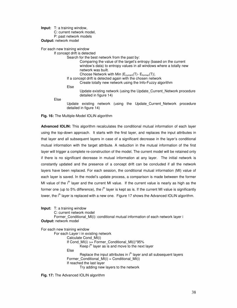
38

Input: T: a training window, C: current network model, P: past network models

Output: network model For each new training window

If concept drift is detected Search for the best network from the past by:

Comparing the value of the target’s entropy (based on the current window’s data) to entropy values in all windows where a totally new network was built. Choose Network with Min |Ecurrent(T)- Eformer(T)|.

If a concept drift is detected again with the chosen network Create totally new network using the Info-Fuzzy algorithm

Else Update existing network (using the Update_Current_Network procedure detailed in figure 14)

Else Update existing network (using the Update_Current_Network procedure detailed in figure 14)

Fig. 16: The Multiple-Model IOLIN algorithm

Advanced IOLIN: This algorithm recalculates the conditional mutual information of each layer

using the top-down approach. It starts with the first layer, and replaces the input attributes in

that layer and all subsequent layers in case of a significant decrease in the layer’s conditional

mutual information with the target attribute. A reduction in the mutual information of the first

layer will trigger a complete re-construction of the model. The current model will be retained only

if there is no significant decrease in mutual information at any layer. The initial network is

constantly updated and the presence of a concept drift can be concluded if all the network

layers have been replaced. For each session, the conditional mutual information (MI) value of

each layer is saved. In the model’s update process, a comparison is made between the former

MI value of the ith layer and the current MI value. If the current value is nearly as high as the

former one (up to 5% difference), the ith layer is kept as is. If the current MI value is significantly

lower, the ith layer is replaced with a new one. Figure 17 shows the Advanced IOLIN algorithm.

Input: T: a training window C: current network model Former_Conditional_MI(i): conditional mutual information of each network layer i

Output: network model For each new training window

For each Layer i in existing network Calculate Cond_MI(i) If Cond_MI(i) >= Former_Conditional_MI(i)*95%

Keep ith

layer as is and move to the next layer Else

Replace the input attributes in ith layer and all subsequent layers

Former_Conditional_MI(i) = Conditional_MI(i) If reached the last layer

Try adding new layers to the network

Fig. 17: The Advanced IOLIN algorithm

39

3.5 Conclusion

In this section we could see a detailed description of a selected set of different algorithms

applied to data streams. Basically, we could see algorithms generating different types of model

representations: trees in the cases of VFDTc, CVFDT and UFFT; ensemble classifiers in the

case of Accuracy-Weighted Ensembles; and info-fuzzy networks in the case of IOLIN. To

process an infinitive stream of items, some algorithms use a sliding window of the most recent

examples like IOLIN, CVFDT and UFFT. Regarding tree models, some algorithms use an

alternative of this model by using functional leaves instead of majority class leaves as the cases

of VFDTc and UFFT.

VFDTc and UFFT use different techniques to select the cut_point used in an inner node for

numerical attributes. In the case of VFDTc, the conditional entropy is used while in UFFT, an

analytical method derived from the quadratic discriminant analysis is used.

For the model building, we could see that VFDTc, UFFT and CVFDT use an information gain

difference (according to Hoeffding bound) to let the tree grows. Accuracy-Weighted Ensembles

build a new classifier and update the weights of the previous classifiers for each new chunk of

data. Finally IOLIN only splits a node in the info-fuzzy network if it gets an improvement in the

conditional mutual information.

The problem of detecting and reacting to concept drift is carried out as follows: VFDTc uses the

sufficient statistics saved to use two different estimators: Drift Detection based on Error

Estimates (EE) and Drift Detection based on Affinity Coefficient (AC). UFFT maintains a Naive

Bayes classifier at each inner node to detect the increase of its online error. CVFDT creates

alternatives sub-trees and when each alternate sub-tree becomes more accurate on new data

than the old one, the old sub-tree is replaced by the new one. Accuracy-Weighted Ensembles

weights each classifier according to the classification error on the most recent chunk of data.

IOLIN computes the difference between training error and testing error.

In figure 18, we can see a summary table with all of this information.

40

Algorithms/features Model representation

Use sliding window

Model building Concept drift detection

UFFT Tree with functional leaves

Yes Use an information gain difference

maintains a Naive Bayes classifier at each inner node

VFDTc Tree with functional leaves

No use an information gain difference

use the sufficient statistics saved to use an estimator

CVFDT Tree Yes use an information gain difference

creates alternatives sub-trees

IOLIN Info-fuzzy network

Yes build a new classifier and update the weights of the previous classifiers for each new chunk of data

computes the difference between training error and testing error

Accuracy-Weighted Ensembles

Ensemble classifiers

No splits a node in the info-fuzzy network if it gets an improvement in the conditional mutual information

weights each classifier according to the classification error

Fig 18: comparative table of evaluated algorithms

41

4 Comparison criteria and performance measures

As we have mentioned previously, this thesis is focused on a benchmarking analysis over a set

of classification algorithms applied to data streams. Since data stream mining has to deal with

new and challenging issues, we think it is appropriate to focus our analysis on these topics.

Basically, we define some points that we want to compare between the algorithms explained in

our previous section. These points cover almost all the characteristic aspects that these types

of algorithms must have:

• Capacity to detect and respond to concept drift: as we mentioned, a concept drift is

a phenomenon produced when the target concept changes because the changes in

some hidden context affecting the target concept. Any algorithm working with data

streams has to detect and react to it adapting its current model to the new concept. We

perform here a graphical comparison. We can plot the model error over the incoming

examples and detect the points in the data stream where a concept drift is produced. In

these points we could analyze how these algorithms detect and react to them.

Basically, the error rate should start to increase until the new model is updated, where

at that time the error rate should decrease or at least get stable. We use different

concept drift levels, from minimal concept drift to abrupt concept drift and see how the

algorithms react.

• Capacity to detect and respond to virtual concept drift: a virtual concept drift is

produced when the underlying data distribution changes, but not the concept target.

Although the concept target may not change, the algorithm needs to adapt to it because

this new data distribution could increase the model error rate. The comparison criteria

used here is similar to the one used in the first point. The only difference is that we

generate data streams with virtual concept drift instead of regular concept drift. Then

we can plot it to see the effects of a virtual drift. Also, we can generate from minimal

virtual concept drift (few changes in the underlying data distribution) to abrupt virtual

concept drift (sudden changes in the underlying data distribution)

• Capacity to detect and respond to recurring concept drift: sometimes the concept

drift may recur. This occurs mostly in seasonal data streams where the data changes

because of changes in a particular temporal variable. Here, we want to measure if

these algorithms react and respond to recurrent drift in a different way than they react to

unseen new drift. We generate here three concept drifts that recur over and over again

in the stream. Then we can compare graphically if they react to a recurring concept drift

different than a new concept drift. Also we can measure which algorithms are more

suitable for these types of concept drift.

• Capacity to adapt to sudden concept drift: as we described in the first measuring

point, there are different concept drift levels. Sudden concept drifts are those changes

that occur abruptly over the stream. We use here the same experiment used for the

42

first measuring point. We want to graphically measure how these algorithms detect and

react to sudden concept drift as these changes occur more abruptly.

• Capacity to adapt to gradual concept drift: this is the opposite measure than sudden

concept drift. We use here the same experiment used for sudden concept drift, but in

this case we measure graphically how these algorithms detect and react to gradual

concept drift as these changes occur more slowly.

• Capacity to adapt to frequent concept drift: both sudden and gradual concept drift

can occur more or less frequently in the stream. This measure analyzes how these

algorithms react as the rate of the changes increases or decreases with the time. We

measure this aspect graphically by increasing the frequency of changes over and over

again and seeing how these algorithms react.

• Accuracy of the classification task: This point measures the accuracy of the models

generated in the training phase. The measures used in the analysis are those derived

from the confusion matrix. A confusion matrix contains information about actual and

predicted classifications done by a classification system [30] as we can see in figure 19.

Predicted Predicted

Negative Positive

Actual Negative a b

Actual Positive c d

Fig 19: Confusion matrix

The entries in the confusion matrix have the following meaning:

a: is the number of correct predictions that an instance is negative

b: is the number of incorrect predictions that an instance is positive

c: is the number of incorrect of predictions that an instance negative

d: is the number of correct predictions that an instance is positive

The measures derived from this matrix that we use are:

Accuracy (AC): the proportion of the total number of predictions that are correct. The

equation is: dcba

daAC

+++

+=

Recall or true positive rate (TP): the proportion of positive cases that are correctly

identified. The equation is: dc

dTP

+=

False positive rate (FP): the proportion of negatives cases that are incorrectly

classified as positive. The equation is: ba

bFP

+=

True negative rate (TN): the proportion of negatives cases that are classified correctly.

The equation is: ba

aTN

+=

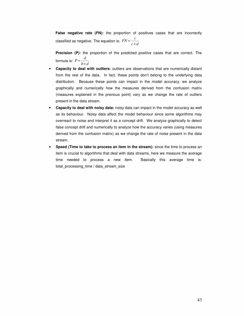
43

False negative rate (FN): the proportion of positives cases that are incorrectly

classified as negative. The equation is: dc

cFN

+=

Precision (P): the proportion of the predicted positive cases that are correct. The

formula is: db

dP

+=

• Capacity to deal with outliers: outliers are observations that are numerically distant

from the rest of the data. In fact, these points don’t belong to the underlying data

distribution. Because these points can impact in the model accuracy, we analyze

graphically and numerically how the measures derived from the confusion matrix

(measures explained in the previous point) vary as we change the rate of outliers

present in the data stream.

• Capacity to deal with noisy data: noisy data can impact in the model accuracy as well

as its behaviour. Noisy data affect the model behaviour since some algorithms may

overreact to noise and interpret it as a concept drift. We analyze graphically to detect

false concept drift and numerically to analyze how the accuracy varies (using measures

derived from the confusion matrix) as we change the rate of noise present in the data

stream.

• Speed (Time to take to process an item in the stream): since the time to process an

item is crucial to algorithms that deal with data streams, here we measure the average

time needed to process a new item. Basically this average time is:

total_processing_time / data_stream_size

44

5 Data sets used in the study

To perform the benchmarking analysis and compute the comparison measures described in the

previous section, we create different data sets based on a moving hyper plane. As we

explained previously, a hyper plane in a d-dimensional space [0; 1]d, is denoted by

� ==

d1i

0ii w xw , where each vector of variables < x1; … ; x d > is a randomly generated instance

and is uniformly distributed. Instances satisfying � >==

d1i

0ii w xw are labelled as positive, and

otherwise negative. This model lets us simulate the different scenarios that we want to test in

this analysis. For example, if we want to generate a concept drift, we just need to change the

coefficients wi. Depending on the changing rate we could generate a sudden (height changing

rate) or a gradual (low changing rate) concept drift. If we want to simulate a virtual concept drift,

we need to change the proportion of items generated on both sides of the hyper plane. For

outliers, we need to generate the vector of variables < x1; … ; x d > with values distant from the

rest of the points. Finally, noise is introduced by randomly switching the labels of p% of the

examples.

To generate the different data sources we use the MOA (Massive Online Analysis) tool [32].

This tool is a framework for learning a data stream from a continuous set of supplied examples.

It includes tools for evaluating a collection of machine learning algorithms as the WEKA project,

but in this case, scaling to more demanding problems. This project is released under GNU

GENERAL PUBLIC LICENSE; it is free and open source. Figure 20 shows a print screen of the

main window of this tool. Basically this tool lets us configure the learner (clicking the

“Configure” button) and run the experiment once we have chosen it (clicking the “Run” button).

In addition this tool comes with an extension called “Concept Drift Stream Generators” that

provides to the tool with many algorithms in charge of generating data sources with concept

drift. In particular, this extension comes with the HyperplaneGenerator algorithm, an

implementation of the moving hyper plane algorithm explained above and used in the

experiment.

From the main window (see Fig. 20), if we click on “Configure” button and select the

HyperplaneGenerator algorithm, we get the configuration window of this algorithm as we can

see in figure 21.

The parameters that we can configure in this algorithm are the followings:

• instanceRandomSeed (default: 1): Seed for random generation of instances.

• numClasses (default: 2): The number of classes to generate.

• numAtts (default: 10): The number of attributes to generate.

• numDriftAtts (default: 2): The number of attributes with drift.

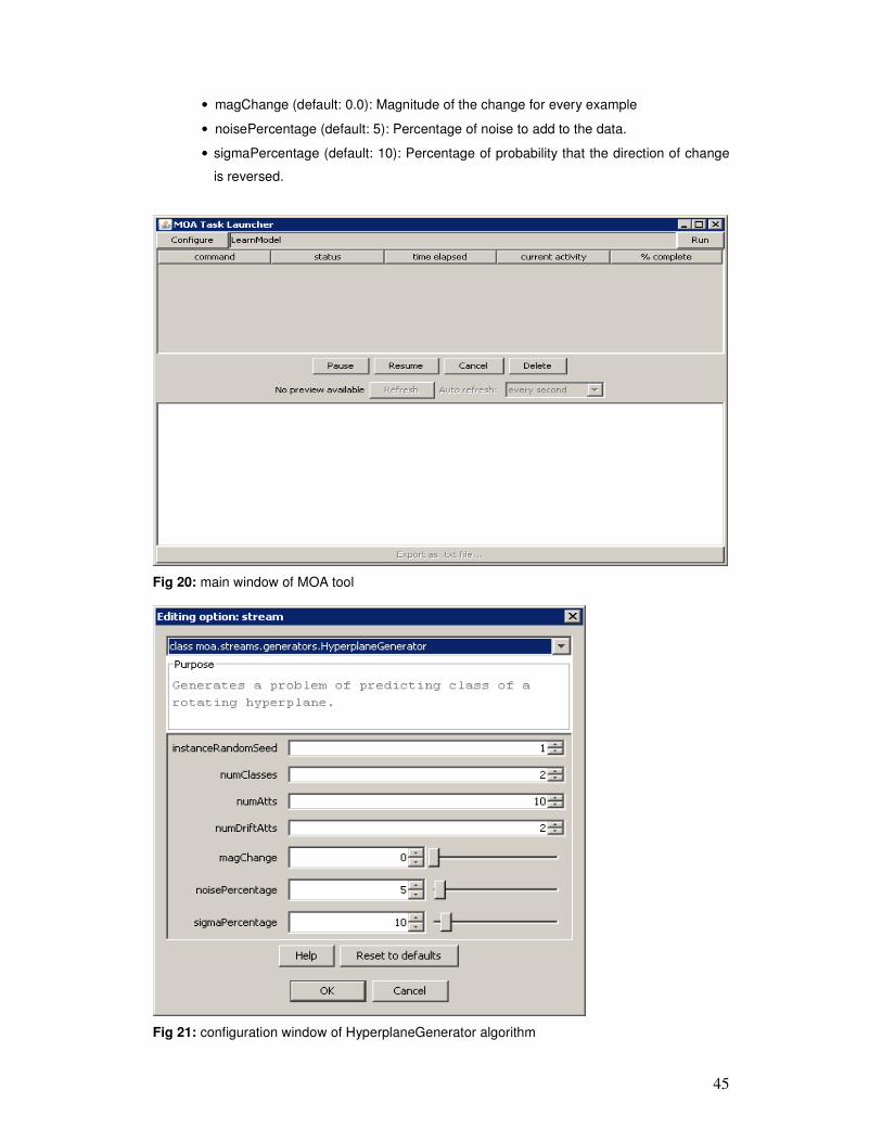
45

• magChange (default: 0.0): Magnitude of the change for every example

• noisePercentage (default: 5): Percentage of noise to add to the data.

• sigmaPercentage (default: 10): Percentage of probability that the direction of change

is reversed.

Fig 20: main window of MOA tool

Fig 21: configuration window of HyperplaneGenerator algorithm

46

Although this tool presents all the configurable parameters used in the moving Hyperplane

algorithm, we added some new ones to cover some aspects needed in our benchmarking

analysis like: outliers, virtual concept drift and concept drift with different frequencies like

sudden concept drift, gradual concept drift and frequent concept drift.

The new parameters added are:

• driftFreq (default: 2): The number of items needed before start of any drift. This attribute

is useful to change the concept drift frequency.

• driftTran (default: 2): The number of items needed in the transition from the old concept to

the new concept. This attribute is useful to generate different types of concept drift, from

sudden to gradual concept drift. The lower this value is the more sudden the concept drift

would be.

• outlierPercentage (default: 1): Percentage of outliers to add to the data.

• distributionPercentage (default: 50): Percentage of probability that the generated attribute

is < 0.5. This attribute is useful to change the underlying data distribution, generating in

this way different type of virtual concept drift.

• magThresholdChange (default: 0): Magnitude of change for the distribution threshold.

The value of this attribute is used to increment the distributionPercentage value each time

a virtual concept drift happen. The bigger this value is the more sudden a virtual concept

drift occur.

In figure 22 we can see the new configuration window associated with the HyperplaneGenerator

algorithm.

The HyperplaneGenerator algorithm lets us generate different datasets for classification

purposes. The main characteristic is the possibility to generate both positive and negative items

separated by a hyper plane. Although this algorithm can generate datasets with more than two

classes, for our analysis we choose the positive-negative approach, that is, a classification task

of two classes. The positive items are those located above the hyper plane and the negative

items are those located below the given hyper plane.

Just to give an example of how the HyperplaneGenerator algorithm can generate the different

types of datasets and how they look like, we present here different datasets generated with

different configurations graphically in scatter plots. All the datasets generated for these

examples have 2 attributes in order to be displayed in a 2-D graphic.

In figure 23 we can see a scatter plot for a dataset of 1000 items with no concept drift, outlier, or

noise.

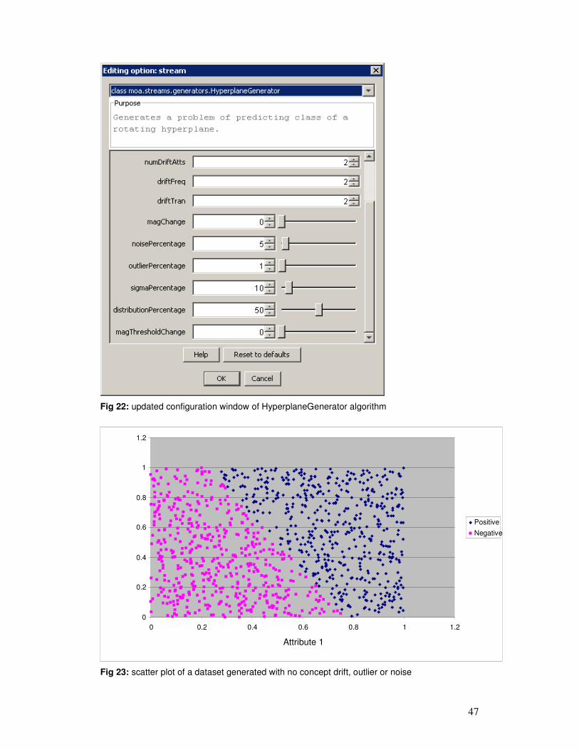
47

Fig 22: updated configuration window of HyperplaneGenerator algorithm

Fig 23: scatter plot of a dataset generated with no concept drift, outlier or noise

0

0.2

0.4

0.6

0.8

1

1.2

0 0.2 0.4 0.6 0.8 1 1.2

Positive

Negative

Attribute 1

48

As we can see in figure 23 above, there is a perfect line that splits up positives and negatives

items. The values of both attributes are in the range of [0, 1] and the distribution between

negative and positive is balanced.

In the next example, we generated a dataset with the same configuration, except that we added

some noise in the data. Specifically for this example, we added 10% noise to the data. We can

see a scatter plot of the generated items in figure 24 below.

Fig 24: scatter plot of a dataset generated with 10% of noisy data

As we can see in figure 24 above, the line that splits up positive and negative items is still there

but there are some items that are wrongly located in the opposite section. That is, some

negative items located above the hyper plane and some positive items located below this hyper

plane. Those items represent the noise added to the HyperplaneGenerator.

Our next example is the capacity to add outliers to the dataset. Each time an outlier item is

needed, an item with values greater than 1 is added to the dataset. For this example we

configured the HyperplaneGenerator with a 1% of outliers. We can see a scatter plot of the

generated items in the figure 25 below.

0

0.2

0.4

0.6

0.8

1

1.2

0 0.2 0.4 0.6 0.8 1 1.2

Positive Negative

Attribute 1

Attri

bute

2

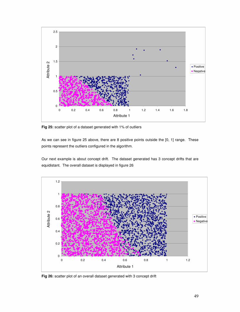
49

Fig 25: scatter plot of a dataset generated with 1% of outliers

As we can see in figure 25 above, there are 8 positive points outside the [0, 1] range. These

points represent the outliers configured in the algorithm.

Our next example is about concept drift. The dataset generated has 3 concept drifts that are

equidistant. The overall dataset is displayed in figure 26

Fig 26: scatter plot of an overall dataset generated with 3 concept drift

0

0.2

0.4

0.6

0.8

1

1.2

0 0.2 0.4 0.6 0.8 1 1.2

Positive

Negative

Attribute 1

Attri

bute

2

0

0.5

1

1.5

2

2.5

0 0.2 0.4 0.6 0.8 1 1.2 1.4 1.6 1.8

Positive Negative

Attribute 1

Att

ribute

2

50

As we can see in figure 26 above, it seems that this dataset was generated with noisy items

since there are items in the opposite section. That is, there are positive items below the hyper

plane and negative items above the hyper plane. In figures 27, 28 and 29 the scatter plots for

the three concepts involved in this example are displayed.

Fig 27: scatter plot of the first concept in a dataset generated with 3 concept drift

Fig 28: scatter plot of the second concept in a dataset generated with 3 concept drift

0.2

0.4

0.6

0.8

1

1.2

0 0.2 0.6 0.8 1 1.2

Positive Negative

Attri

bu

te 2

Attribute 1

0

0.2

0.4

0.6

0.8

1

1.2

0 0.2 0.4 0.6 0.8 1 1.2

Positive Negative

Att

ribute

2

Attribute 1

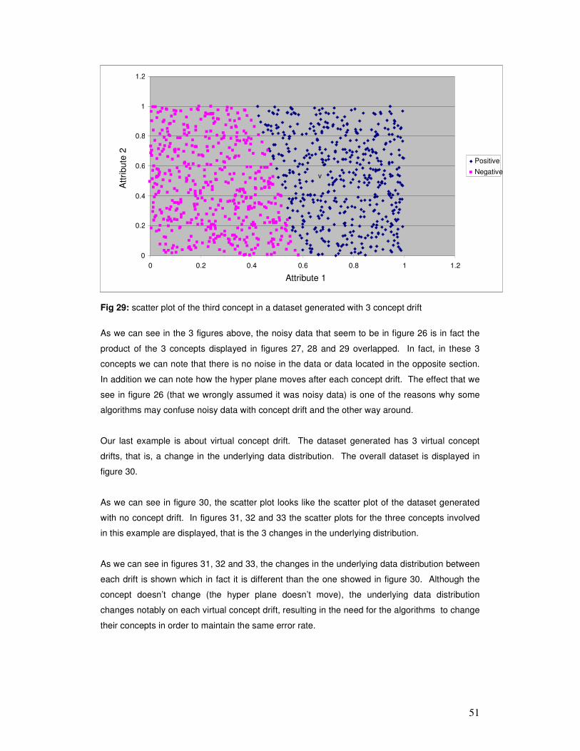
51

Fig 29: scatter plot of the third concept in a dataset generated with 3 concept drift

As we can see in the 3 figures above, the noisy data that seem to be in figure 26 is in fact the

product of the 3 concepts displayed in figures 27, 28 and 29 overlapped. In fact, in these 3

concepts we can note that there is no noise in the data or data located in the opposite section.

In addition we can note how the hyper plane moves after each concept drift. The effect that we

see in figure 26 (that we wrongly assumed it was noisy data) is one of the reasons why some

algorithms may confuse noisy data with concept drift and the other way around.

Our last example is about virtual concept drift. The dataset generated has 3 virtual concept

drifts, that is, a change in the underlying data distribution. The overall dataset is displayed in

figure 30.

As we can see in figure 30, the scatter plot looks like the scatter plot of the dataset generated

with no concept drift. In figures 31, 32 and 33 the scatter plots for the three concepts involved

in this example are displayed, that is the 3 changes in the underlying distribution.

As we can see in figures 31, 32 and 33, the changes in the underlying data distribution between

each drift is shown which in fact it is different than the one showed in figure 30. Although the

concept doesn’t change (the hyper plane doesn’t move), the underlying data distribution

changes notably on each virtual concept drift, resulting in the need for the algorithms to change

their concepts in order to maintain the same error rate.

0

0.2

0.4

0.6

0.8

1

1.2

0 0.2 0.4 0.6 0.8 1 1.2

Positive Negative

v

Attribute 1

Att

ribute

2

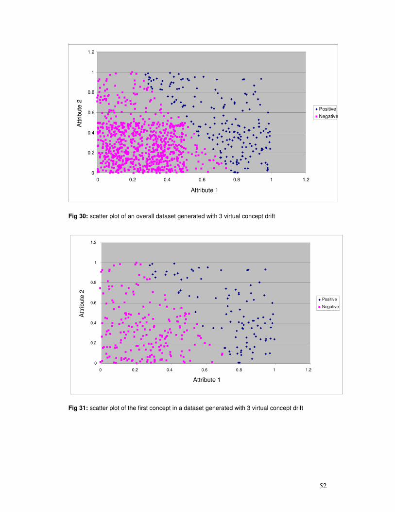
52

Fig 30: scatter plot of an overall dataset generated with 3 virtual concept drift

Fig 31: scatter plot of the first concept in a dataset generated with 3 virtual concept drift

0

0.2

0.4

0.6

0.8

1

1.2

0 0.2 0.4 0.6 0.8 1 1.2

Positive

Negative

Attribute 1

Attri

bute

2

0

0.2

0.4

0.6

0.8

1

1.2

0 0.2 0.4 0.6 0.8 1 1.2

Positive Negative

Attribute 1

Att

ribute

2

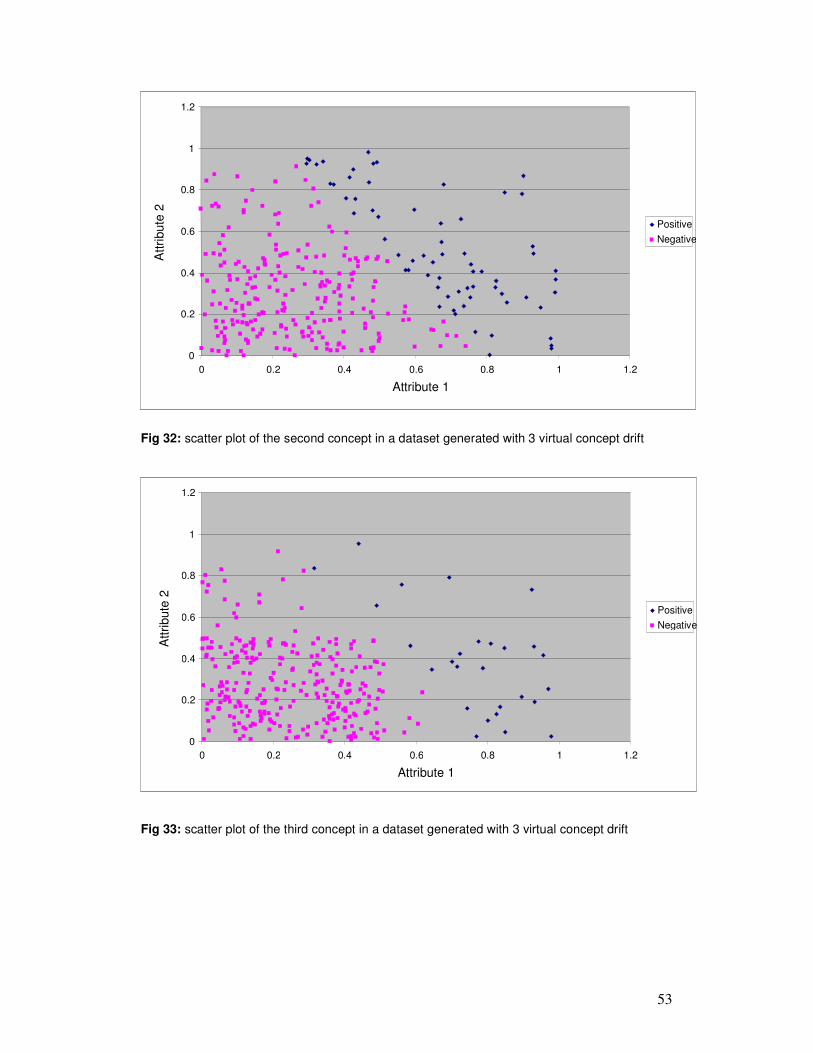
53

Fig 32: scatter plot of the second concept in a dataset generated with 3 virtual concept drift

Fig 33: scatter plot of the third concept in a dataset generated with 3 virtual concept drift

0

0.2

0.4

0.6

0.8

1

1.2

0 0.2 0.4 0.6 0.8 1 1.2

Positive Negative

Attribute 1

Attri

bute

2

0

0.2

0.4

0.6

0.8

1

1.2

0 0.2 0.4 0.6 0.8 1 1.2

Positive Negative

Attribute 1

Attri

bute

2

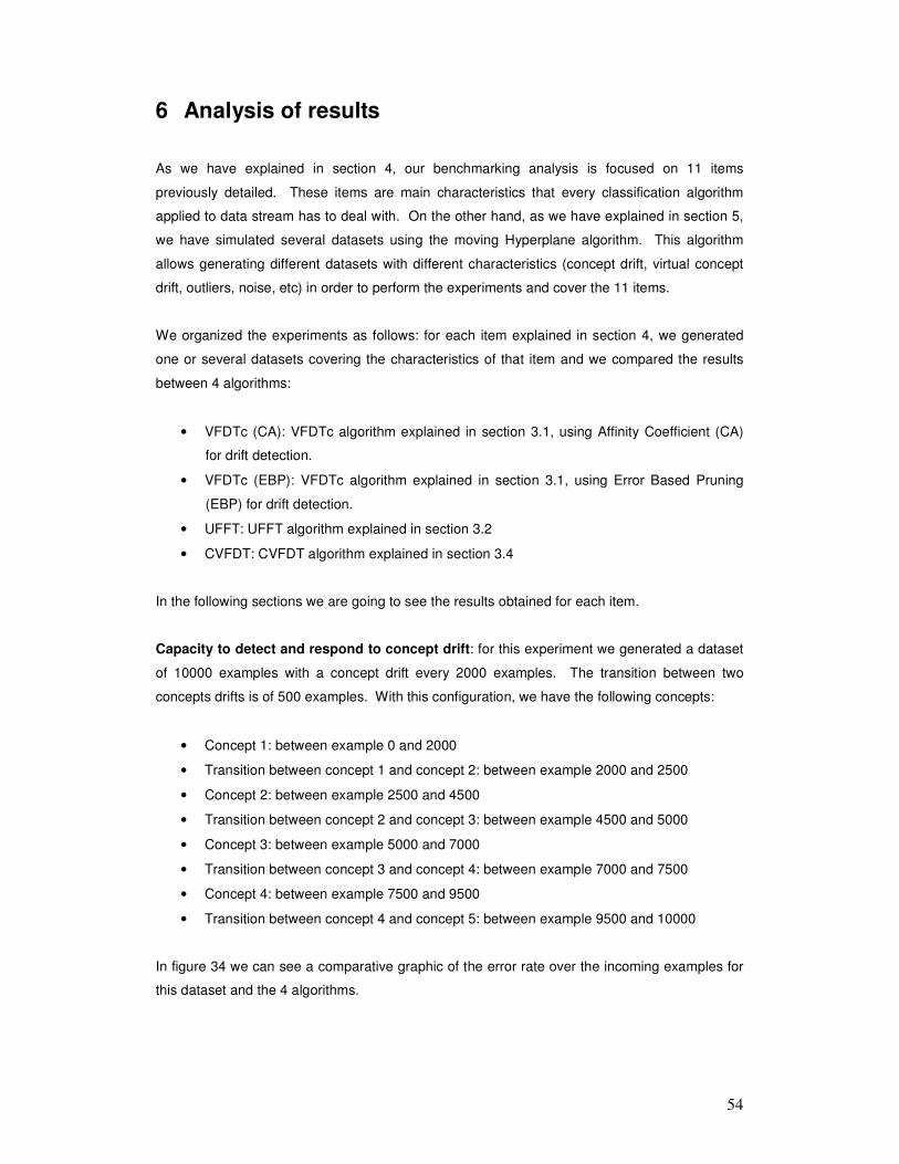
54

6 Analysis of results

As we have explained in section 4, our benchmarking analysis is focused on 11 items

previously detailed. These items are main characteristics that every classification algorithm

applied to data stream has to deal with. On the other hand, as we have explained in section 5,

we have simulated several datasets using the moving Hyperplane algorithm. This algorithm

allows generating different datasets with different characteristics (concept drift, virtual concept

drift, outliers, noise, etc) in order to perform the experiments and cover the 11 items.

We organized the experiments as follows: for each item explained in section 4, we generated

one or several datasets covering the characteristics of that item and we compared the results

between 4 algorithms:

• VFDTc (CA): VFDTc algorithm explained in section 3.1, using Affinity Coefficient (CA)

for drift detection.

• VFDTc (EBP): VFDTc algorithm explained in section 3.1, using Error Based Pruning

(EBP) for drift detection.

• UFFT: UFFT algorithm explained in section 3.2

• CVFDT: CVFDT algorithm explained in section 3.4

In the following sections we are going to see the results obtained for each item.

Capacity to detect and respond to concept drift: for this experiment we generated a dataset

of 10000 examples with a concept drift every 2000 examples. The transition between two

concepts drifts is of 500 examples. With this configuration, we have the following concepts:

• Concept 1: between example 0 and 2000

• Transition between concept 1 and concept 2: between example 2000 and 2500

• Concept 2: between example 2500 and 4500

• Transition between concept 2 and concept 3: between example 4500 and 5000

• Concept 3: between example 5000 and 7000

• Transition between concept 3 and concept 4: between example 7000 and 7500

• Concept 4: between example 7500 and 9500

• Transition between concept 4 and concept 5: between example 9500 and 10000

In figure 34 we can see a comparative graphic of the error rate over the incoming examples for

this dataset and the 4 algorithms.

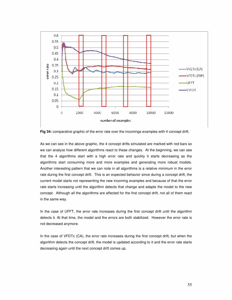
55

Fig 34: comparative graphic of the error rate over the incomings examples with 4 concept drift.

As we can see in the above graphic, the 4 concept drifts simulated are marked with red bars so

we can analyze how different algorithms react to these changes. At the beginning, we can see

that the 4 algorithms start with a high error rate and quickly it starts decreasing as the

algorithms start consuming more and more examples and generating more robust models.

Another interesting pattern that we can note in all algorithms is a relative minimum in the error

rate during the first concept drift. This is an expected behavior since during a concept drift, the

current model starts not representing the new incoming examples and because of that the error

rate starts increasing until the algorithm detects that change and adapts the model to the new

concept. Although all the algorithms are affected for the first concept drift, not all of them react

in the same way.

In the case of UFFT, the error rate increases during the first concept drift until the algorithm

detects it. At that time, the model and the errors are both stabilized. However the error rate is

not decreased anymore.

In the case of VFDTc (CA), the error rate increases during the first concept drift, but when the

algorithm detects the concept drift, the model is updated according to it and the error rate starts

decreasing again until the next concept drift comes up.

56

In the case of VFDTc (EBP), the error rate increases during the first concept drift until the

algorithm detects it and the model is stabilized and so the error rate. However the error rate is

not decreased in the short term and just smoothly after seeing so many examples.

In the case of CVFDT, the error rate increases during the first concept drift but when the

algorithm reacts and updates the model, it starts decreasing continuously, not being affected by

subsequent concept drifts.

If we analyze not just the first concept drift, but the later ones, we detect that they just affect

VFDTc (CA), that is, VFDTc (CA) is the only algorithm that its error rate increases during each

concept drift. Although all of them affect the model, we can note that as new concept drifts

come up, their effects becomes less and less.

Finally, we can point out that although UFFT performs better over the examples, VFDTc (CA)

and CVFDT are the best algorithms for reacting and adapting to the new concept, that is, they

reduce the error rate after adapting to the new examples.

Capacity to detect and respond to virtual concept drift: for this experiment we generated

different datasets of 10000 examples with a virtual concept drift every 2000 examples and

varying the number of examples seen in the transition between two concepts. This way, we can

analyze how the algorithms react from minimal virtual concept drift (few examples in the

transition between two concepts) to sudden virtual concept drift (lot of examples in the transition

between two concepts). We generated the following transitions from minimal to sudden:

• drift 100: 100 examples in the transition between concepts

• drift 50: 50 examples in the transition between concepts

• drift 40: 40 examples in the transition between concepts

• drift 20: 20 examples in the transition between concepts

• drift 10: 10 examples in the transition between concepts

In figure 35 we can see a comparative graphic of the error rate over the incoming examples for

the datasets with different virtual concept drift transition for VFDTc (CA) algorithm. It is

important to note that the algorithm is robust to changes in the concept drift transition, because,

as we can see in the comparative graphic, the error rate in all of the datasets follows the same

trend. So we can state that the type of virtual drift is not affecting the algorithm. On the other

hand we can note that the error rate is high at the beginning but then it goes down as new

examples are seen. For that reason we can conclude that the algorithm is not being affected by

successive virtual concept drifts.

57

Fig 35: comparative graphic of virtual concept drifts for VFDTc (CA).

If we compare the results for VFDTc (CA) in figure 35 with the ones for VFDTc (EBP) in figure

36, we can observe similar values and trends. For that reason, we can conclude that VFDTc

(EBP) is robust to changes in the concept drift transition and is not being affected by successive

virtual concept drift. Actually we can note that both 35 and 36 plots are very similar as well as

the overall performance. So for this we can conclude that the concept drift detection algorithms

for VFDTc (in this case CA and EBP) are not affected by virtual concept drift.

Fig 36: comparative graphic of virtual concept drifts for VFDTc (EBP).

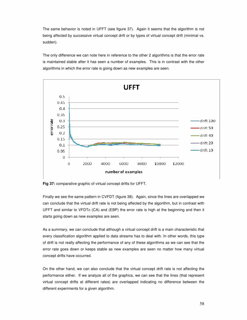
58

The same behavior is noted in UFFT (see figure 37). Again it seems that the algorithm is not

being affected by successive virtual concept drift or by types of virtual concept drift (minimal vs.

sudden).

The only difference we can note here in reference to the other 2 algorithms is that the error rate

is maintained stable after it has seen a number of examples. This is in contrast with the other

algorithms in which the error rate is going down as new examples are seen.

Fig 37: comparative graphic of virtual concept drifts for UFFT.

Finally we see the same pattern in CVFDT (figure 38). Again, since the lines are overlapped we

can conclude that the virtual drift rate is not being affected by the algorithm, but in contrast with

UFFT and similar to VFDTc (CA) and (EBP) the error rate is high at the beginning and then it

starts going down as new examples are seen.

As a summary, we can conclude that although a virtual concept drift is a main characteristic that

every classification algorithm applied to data streams has to deal with. In other words, this type

of drift is not really affecting the performance of any of these algorithms as we can see that the

error rate goes down or keeps stable as new examples are seen no matter how many virtual

concept drifts have occurred.

On the other hand, we can also conclude that the virtual concept drift rate is not affecting the

performance either. If we analyze all of the graphics, we can see that the lines (that represent

virtual concept drifts at different rates) are overlapped indicating no difference between the

different experiments for a given algorithm.

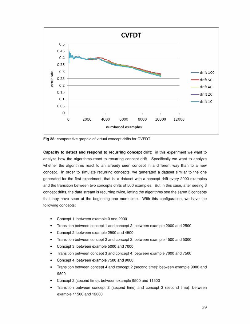
59

Fig 38: comparative graphic of virtual concept drifts for CVFDT.

Capacity to detect and respond to recurring concept drift: in this experiment we want to

analyze how the algorithms react to recurring concept drift. Specifically we want to analyze

whether the algorithms react to an already seen concept in a different way than to a new

concept. In order to simulate recurring concepts, we generated a dataset similar to the one

generated for the first experiment, that is, a dataset with a concept drift every 2000 examples

and the transition between two concepts drifts of 500 examples. But in this case, after seeing 3

concept drifts, the data stream is recurring twice, letting the algorithms see the same 3 concepts

that they have seen at the beginning one more time. With this configuration, we have the

following concepts:

• Concept 1: between example 0 and 2000

• Transition between concept 1 and concept 2: between example 2000 and 2500

• Concept 2: between example 2500 and 4500

• Transition between concept 2 and concept 3: between example 4500 and 5000

• Concept 3: between example 5000 and 7000

• Transition between concept 3 and concept 4: between example 7000 and 7500

• Concept 4: between example 7500 and 9000

• Transition between concept 4 and concept 2 (second time): between example 9000 and

9500

• Concept 2 (second time): between example 9500 and 11500

• Transition between concept 2 (second time) and concept 3 (second time): between

example 11500 and 12000

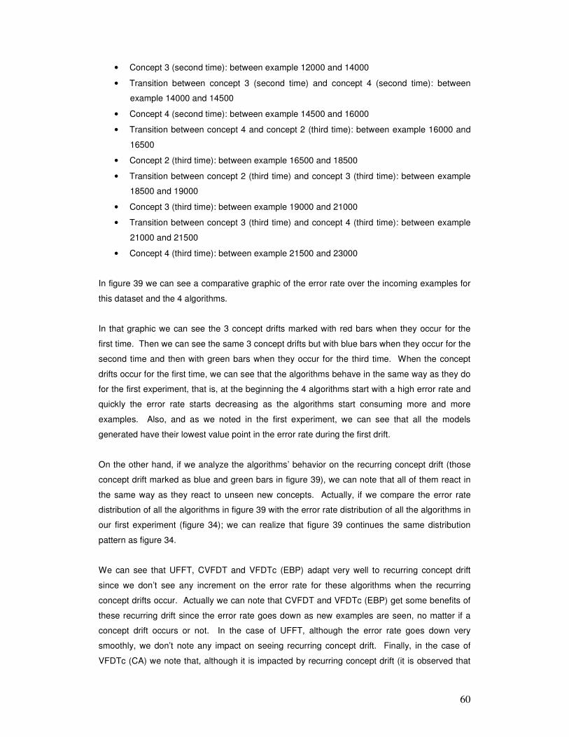
60

• Concept 3 (second time): between example 12000 and 14000

• Transition between concept 3 (second time) and concept 4 (second time): between

example 14000 and 14500

• Concept 4 (second time): between example 14500 and 16000

• Transition between concept 4 and concept 2 (third time): between example 16000 and

16500

• Concept 2 (third time): between example 16500 and 18500

• Transition between concept 2 (third time) and concept 3 (third time): between example

18500 and 19000

• Concept 3 (third time): between example 19000 and 21000

• Transition between concept 3 (third time) and concept 4 (third time): between example

21000 and 21500

• Concept 4 (third time): between example 21500 and 23000

In figure 39 we can see a comparative graphic of the error rate over the incoming examples for

this dataset and the 4 algorithms.

In that graphic we can see the 3 concept drifts marked with red bars when they occur for the

first time. Then we can see the same 3 concept drifts but with blue bars when they occur for the

second time and then with green bars when they occur for the third time. When the concept

drifts occur for the first time, we can see that the algorithms behave in the same way as they do

for the first experiment, that is, at the beginning the 4 algorithms start with a high error rate and

quickly the error rate starts decreasing as the algorithms start consuming more and more

examples. Also, and as we noted in the first experiment, we can see that all the models

generated have their lowest value point in the error rate during the first drift.

On the other hand, if we analyze the algorithms’ behavior on the recurring concept drift (those

concept drift marked as blue and green bars in figure 39), we can note that all of them react in

the same way as they react to unseen new concepts. Actually, if we compare the error rate

distribution of all the algorithms in figure 39 with the error rate distribution of all the algorithms in

our first experiment (figure 34); we can realize that figure 39 continues the same distribution

pattern as figure 34.

We can see that UFFT, CVFDT and VFDTc (EBP) adapt very well to recurring concept drift

since we don’t see any increment on the error rate for these algorithms when the recurring

concept drifts occur. Actually we can note that CVFDT and VFDTc (EBP) get some benefits of

these recurring drift since the error rate goes down as new examples are seen, no matter if a

concept drift occurs or not. In the case of UFFT, although the error rate goes down very

smoothly, we don’t note any impact on seeing recurring concept drift. Finally, in the case of

VFDTc (CA) we note that, although it is impacted by recurring concept drift (it is observed that

61

the error rate increases on every concept drift), the algorithm reacts to recurring concept drift in

the same way as unseen concept drift, that is, the algorithm doesn’t deal previously seen

concept in any special way. Again, we note that the increment on the error rate is smoother as

new concept drifts are seen.

Fig 39: comparative graphic of the error rate over the incomings examples for recurring concept

drifts.

Capacity to adapt to sudden concept drift: in real data stream scenarios, the concept drifts

can occur with different change rates, from gradual concept drift (smooth changes in the

concept) to sudden concept drift (abrupt changes high rates). In this experiment we analyze

how the algorithms react to concept drift as they become more and more abrupt. For analyzing

this, we generated different datasets of 10000 examples with a concept drift every 2000

examples and varying the numbers of examples seen in the transition between two concepts.

With this configuration, we generated the following datasets:

• drift 100: 100 examples in the transition between concepts

• drift 50: 50 examples in the transition between concepts

• drift 40: 40 examples in the transition between concepts

• drift 20: 20 examples in the transition between concepts

• drift 10: 10 examples in the transition between concepts

In figure 40 we can see a comparative graphic of the error rate over the incoming examples for

the datasets with different sudden change rate for VFDTc (CA) algorithm.

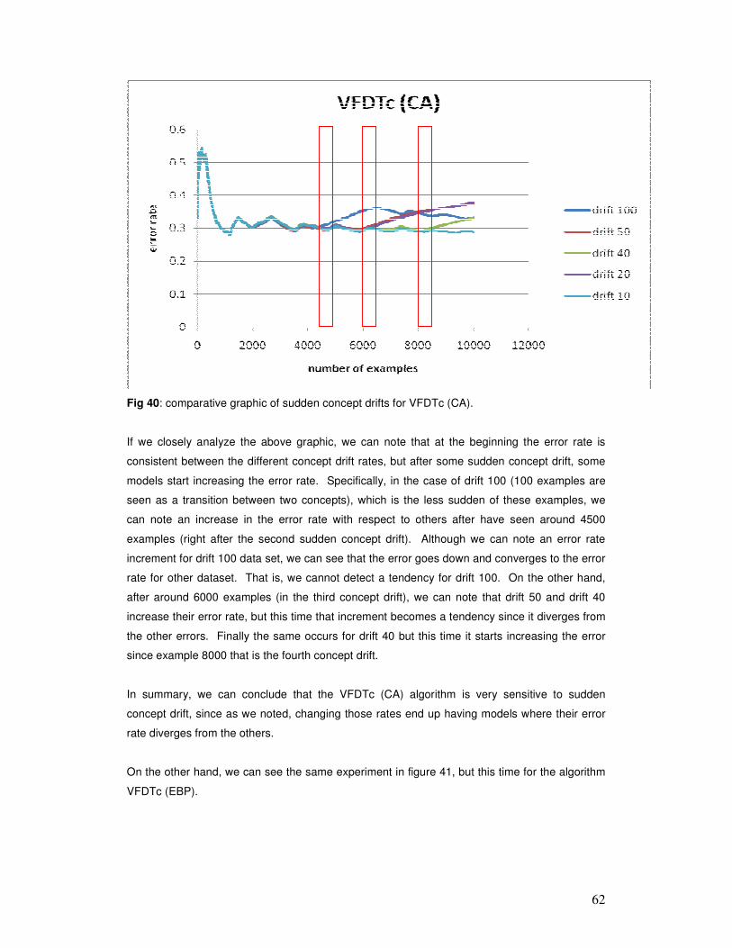
62

Fig 40: comparative graphic of sudden concept drifts for VFDTc (CA).

If we closely analyze the above graphic, we can note that at the beginning the error rate is

consistent between the different concept drift rates, but after some sudden concept drift, some

models start increasing the error rate. Specifically, in the case of drift 100 (100 examples are

seen as a transition between two concepts), which is the less sudden of these examples, we

can note an increase in the error rate with respect to others after have seen around 4500

examples (right after the second sudden concept drift). Although we can note an error rate

increment for drift 100 data set, we can see that the error goes down and converges to the error

rate for other dataset. That is, we cannot detect a tendency for drift 100. On the other hand,

after around 6000 examples (in the third concept drift), we can note that drift 50 and drift 40

increase their error rate, but this time that increment becomes a tendency since it diverges from

the other errors. Finally the same occurs for drift 40 but this time it starts increasing the error

since example 8000 that is the fourth concept drift.

In summary, we can conclude that the VFDTc (CA) algorithm is very sensitive to sudden

concept drift, since as we noted, changing those rates end up having models where their error

rate diverges from the others.

On the other hand, we can see the same experiment in figure 41, but this time for the algorithm

VFDTc (EBP).

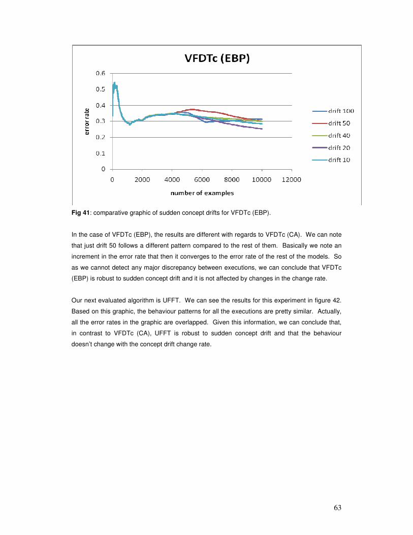
63

Fig 41: comparative graphic of sudden concept drifts for VFDTc (EBP).

In the case of VFDTc (EBP), the results are different with regards to VFDTc (CA). We can note

that just drift 50 follows a different pattern compared to the rest of them. Basically we note an

increment in the error rate that then it converges to the error rate of the rest of the models. So

as we cannot detect any major discrepancy between executions, we can conclude that VFDTc

(EBP) is robust to sudden concept drift and it is not affected by changes in the change rate.

Our next evaluated algorithm is UFFT. We can see the results for this experiment in figure 42.

Based on this graphic, the behaviour patterns for all the executions are pretty similar. Actually,

all the error rates in the graphic are overlapped. Given this information, we can conclude that,

in contrast to VFDTc (CA), UFFT is robust to sudden concept drift and that the behaviour

doesn’t change with the concept drift change rate.

64

Fig 42: comparative graphic of sudden concept drifts for UFFT.

Finally in figure 43, we can see the same results but this time for CVFDT. Again, and similar to

UFFT and VFDTc (EBP), although there are some discrepancies between the different

executions (for instance, drift 50 and drift 100 increase their error rate after seeing around 4000

examples), all these discrepancies converges to the behavioural pattern so we can conclude

here too that CVFDT is robust to sudden concept drift.

Fig 43: comparative graphic of sudden concept drifts for CVFDT.

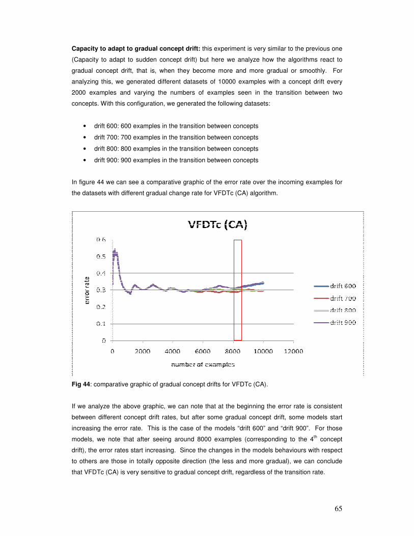
65

Capacity to adapt to gradual concept drift: this experiment is very similar to the previous one

(Capacity to adapt to sudden concept drift) but here we analyze how the algorithms react to

gradual concept drift, that is, when they become more and more gradual or smoothly. For

analyzing this, we generated different datasets of 10000 examples with a concept drift every

2000 examples and varying the numbers of examples seen in the transition between two

concepts. With this configuration, we generated the following datasets:

• drift 600: 600 examples in the transition between concepts

• drift 700: 700 examples in the transition between concepts

• drift 800: 800 examples in the transition between concepts

• drift 900: 900 examples in the transition between concepts

In figure 44 we can see a comparative graphic of the error rate over the incoming examples for

the datasets with different gradual change rate for VFDTc (CA) algorithm.

Fig 44: comparative graphic of gradual concept drifts for VFDTc (CA).

If we analyze the above graphic, we can note that at the beginning the error rate is consistent

between different concept drift rates, but after some gradual concept drift, some models start

increasing the error rate. This is the case of the models “drift 600” and “drift 900”. For those

models, we note that after seeing around 8000 examples (corresponding to the 4th concept

drift), the error rates start increasing. Since the changes in the models behaviours with respect

to others are those in totally opposite direction (the less and more gradual), we can conclude

that VFDTc (CA) is very sensitive to gradual concept drift, regardless of the transition rate.

66

Actually, if we compare this conclusion with the one elaborated for sudden concept drift, we

realize that the algorithm is very sensitive to both gradual and sudden concept drift. The only

difference between the two is that the algorithm seems to behave stable for more time in

gradual concept drift. If we compare the pattern in figure 44 vs. the one in figure 40, we can

note that in sudden concept drift, some models start being unstable on the 2nd

concept drift

while in gradual concept drift, this happens on the 4th concept drift. But sooner or later, the

process becomes unstable no matter what change occurs in the transition rate.

In figure 45 we can see a comparative graphic of the error rate over the incoming examples for

the datasets with different gradual change rate for VFDTc (EBP) algorithm.

Fig 45: comparative graphic of gradual concept drifts for VFDTc (EBP).

In this case, we can note that the lines associated with each concept drift rate are almost

overlapped, meaning that the algorithm doesn’t suffer a huge impact changing the change rate.

Actually it behaves very strong over these change rates.

Again, if we compare these conclusions with the one for sudden concept drift, we detected that

in both cases the algorithm behaves very robust to changes in the rate even if they become

more and more sudden or more and more gradual. Therefore, we can conclude that VFDTc

(EBP), in contrast with VFDTc (CA), performs very similar although the concept drift transition

rate is changed.

Our next evaluated algorithm is UFFT. We can see the results for this experiment in figure 46.

Here we can see similar results compared to the one obtained for VFDTc (EBP). That is, the

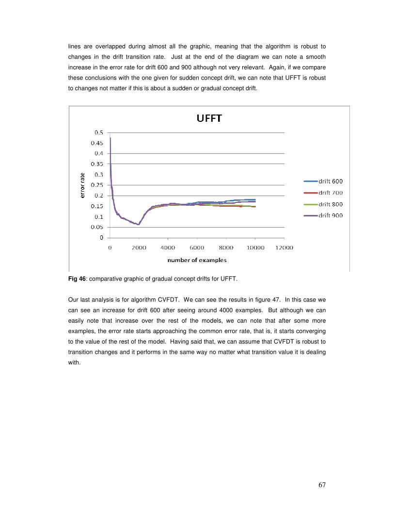
67

lines are overlapped during almost all the graphic, meaning that the algorithm is robust to

changes in the drift transition rate. Just at the end of the diagram we can note a smooth

increase in the error rate for drift 600 and 900 although not very relevant. Again, if we compare

these conclusions with the one given for sudden concept drift, we can note that UFFT is robust

to changes not matter if this is about a sudden or gradual concept drift.

Fig 46: comparative graphic of gradual concept drifts for UFFT.

Our last analysis is for algorithm CVFDT. We can see the results in figure 47. In this case we

can see an increase for drift 600 after seeing around 4000 examples. But although we can

easily note that increase over the rest of the models, we can note that after some more

examples, the error rate starts approaching the common error rate, that is, it starts converging

to the value of the rest of the model. Having said that, we can assume that CVFDT is robust to

transition changes and it performs in the same way no matter what transition value it is dealing

with.

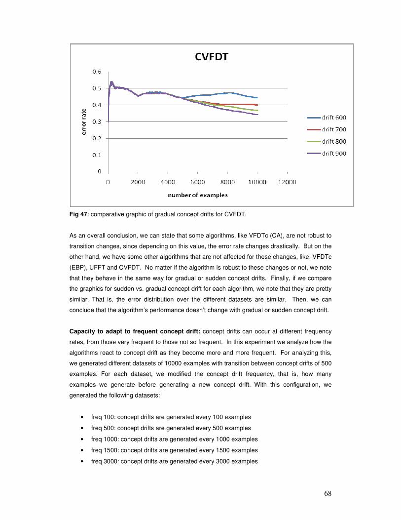
68

Fig 47: comparative graphic of gradual concept drifts for CVFDT.

As an overall conclusion, we can state that some algorithms, like VFDTc (CA), are not robust to

transition changes, since depending on this value, the error rate changes drastically. But on the

other hand, we have some other algorithms that are not affected for these changes, like: VFDTc

(EBP), UFFT and CVFDT. No matter if the algorithm is robust to these changes or not, we note

that they behave in the same way for gradual or sudden concept drifts. Finally, if we compare

the graphics for sudden vs. gradual concept drift for each algorithm, we note that they are pretty

similar, That is, the error distribution over the different datasets are similar. Then, we can

conclude that the algorithm’s performance doesn’t change with gradual or sudden concept drift.

Capacity to adapt to frequent concept drift: concept drifts can occur at different frequency

rates, from those very frequent to those not so frequent. In this experiment we analyze how the

algorithms react to concept drift as they become more and more frequent. For analyzing this,

we generated different datasets of 10000 examples with transition between concept drifts of 500

examples. For each dataset, we modified the concept drift frequency, that is, how many

examples we generate before generating a new concept drift. With this configuration, we

generated the following datasets:

• freq 100: concept drifts are generated every 100 examples

• freq 500: concept drifts are generated every 500 examples

• freq 1000: concept drifts are generated every 1000 examples

• freq 1500: concept drifts are generated every 1500 examples

• freq 3000: concept drifts are generated every 3000 examples

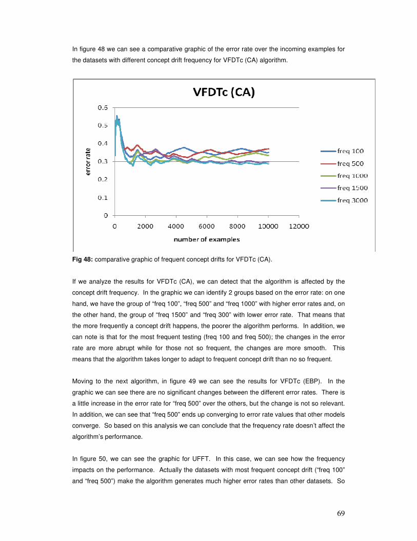
69

In figure 48 we can see a comparative graphic of the error rate over the incoming examples for

the datasets with different concept drift frequency for VFDTc (CA) algorithm.

Fig 48: comparative graphic of frequent concept drifts for VFDTc (CA).

If we analyze the results for VFDTc (CA), we can detect that the algorithm is affected by the

concept drift frequency. In the graphic we can identify 2 groups based on the error rate: on one

hand, we have the group of “freq 100”, “freq 500” and “freq 1000” with higher error rates and, on

the other hand, the group of “freq 1500” and “freq 300” with lower error rate. That means that

the more frequently a concept drift happens, the poorer the algorithm performs. In addition, we

can note is that for the most frequent testing (freq 100 and freq 500); the changes in the error

rate are more abrupt while for those not so frequent, the changes are more smooth. This

means that the algorithm takes longer to adapt to frequent concept drift than no so frequent.

Moving to the next algorithm, in figure 49 we can see the results for VFDTc (EBP). In the

graphic we can see there are no significant changes between the different error rates. There is

a little increase in the error rate for “freq 500” over the others, but the change is not so relevant.

In addition, we can see that “freq 500” ends up converging to error rate values that other models

converge. So based on this analysis we can conclude that the frequency rate doesn’t affect the

algorithm’s performance.

In figure 50, we can see the graphic for UFFT. In this case, we can see how the frequency

impacts on the performance. Actually the datasets with most frequent concept drift (“freq 100”

and “freq 500”) make the algorithm generates much higher error rates than other datasets. So

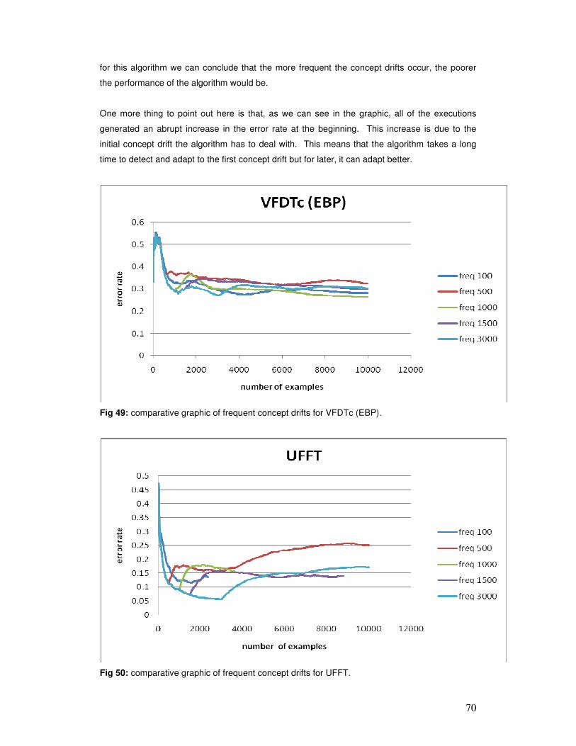
70

for this algorithm we can conclude that the more frequent the concept drifts occur, the poorer

the performance of the algorithm would be.

One more thing to point out here is that, as we can see in the graphic, all of the executions

generated an abrupt increase in the error rate at the beginning. This increase is due to the

initial concept drift the algorithm has to deal with. This means that the algorithm takes a long

time to detect and adapt to the first concept drift but for later, it can adapt better.

Fig 49: comparative graphic of frequent concept drifts for VFDTc (EBP).

Fig 50: comparative graphic of frequent concept drifts for UFFT.

71

The last algorithm for this experiment is CVFDT. We can see the result in figure 51.

Fig 51: comparative graphic of frequent concept drifts for CVFDT.

In this case, although we can note that the error rates vary over the different datasets, we can

note that all of the error rates end up converging to similar values. This means that in the long-

term (after seeing a lot of examples) the algorithm is not affected by the changes in the

frequency.

Accuracy of the classification task: in this experiment we want to measure the overall

accuracy of the models generated by the algorithms. To understand this better, we are going to

use a confusion matrix detailed in figure 19 and all the measures derived from it. For this

experiment we generated a dataset of 10000 examples with no concept drifts. In order to

generate more robust measures, we tested the models using a cross-validation method with 5

folds. So for each of the 5 executions on each algorithm, we used 8000 examples for training

and 2000 for testing. Then an average of these 5 executions are averaged and shown in this

experiment.

In figure 52 we can see the confusion matrix for VFDTc (CA)

Predicted Predicted

Class 1 Class 2

Actual Class 1 887 109

Actual Class 2 101 903

Fig 52: Confusion matrix for VFDTc (CA)

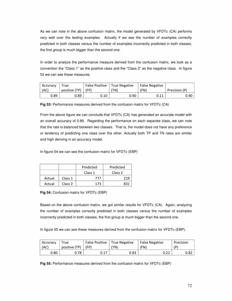
72

As we can note in the above confusion matrix, the model generated by VFDTc (CA) performs

very well over the testing examples. Actually if we see the number of examples correctly

predicted in both classes versus the number of examples incorrectly predicted in both classes,

the first group is much bigger than the second one.

In order to analyze the performance measure derived from the confusion matrix, we took as a

convention the “Class 1” as the positive class and the “Class 2” as the negative class. In figure

53 we can see these measures.

Accuracy

(AC)

True

positive (TP)

False Positive

(FP)

True Negative

(TN)

False Negative

(FN) Precision (P)

0.89 0.89 0.10 0.90 0.11 0.90

Fig 53: Performance measures derived from the confusion matrix for VFDTc (CA)

From the above figure we can conclude that VFDTc (CA) has generated an accurate model with

an overall accuracy of 0.89. Regarding the performance on each separate class, we can note

that the rate is balanced between two classes. That is, the model does not have any preference

or tendency of predicting one class over the other. Actually both TP and TN rates are similar

and high deriving in an accuracy model.

In figure 54 we can see the confusion matrix for VFDTc (EBP)

Predicted Predicted

Class 1 Class 2

Actual Class 1 777 219

Actual Class 2 173 831

Fig 54: Confusion matrix for VFDTc (EBP)

Based on the above confusion matrix, we got similar results for VFDTc (CA). Again, analyzing

the number of examples correctly predicted in both classes versus the number of examples

incorrectly predicted in both classes, the first group is much bigger than the second one.

In figure 55 we can see these measures derived from the confusion matrix for VFDTc (EBP).

Accuracy

(AC)

True

positive (TP)

False Positive

(FP)

True Negative

(TN)

False Negative

(FN)

Precision

(P)

0.80 0.78 0.17 0.83 0.22 0.82

Fig 55: Performance measures derived from the confusion matrix for VFDTc (EBP)

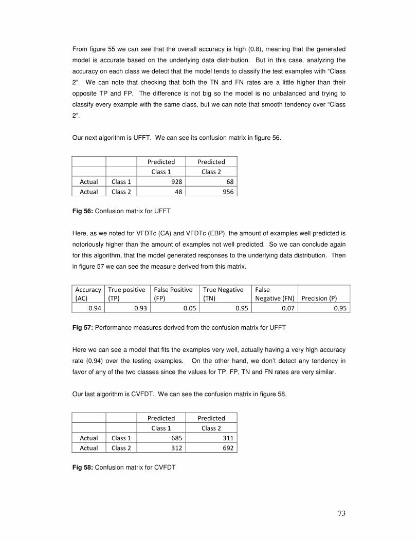
73

From figure 55 we can see that the overall accuracy is high (0.8), meaning that the generated

model is accurate based on the underlying data distribution. But in this case, analyzing the

accuracy on each class we detect that the model tends to classify the test examples with “Class

2”. We can note that checking that both the TN and FN rates are a little higher than their

opposite TP and FP. The difference is not big so the model is no unbalanced and trying to

classify every example with the same class, but we can note that smooth tendency over “Class

2”.

Our next algorithm is UFFT. We can see its confusion matrix in figure 56.

Predicted Predicted

Class 1 Class 2

Actual Class 1 928 68

Actual Class 2 48 956

Fig 56: Confusion matrix for UFFT

Here, as we noted for VFDTc (CA) and VFDTc (EBP), the amount of examples well predicted is

notoriously higher than the amount of examples not well predicted. So we can conclude again

for this algorithm, that the model generated responses to the underlying data distribution. Then

in figure 57 we can see the measure derived from this matrix.

Accuracy

(AC)

True positive

(TP)

False Positive

(FP)

True Negative

(TN)

False

Negative (FN) Precision (P)

0.94 0.93 0.05 0.95 0.07 0.95

Fig 57: Performance measures derived from the confusion matrix for UFFT

Here we can see a model that fits the examples very well, actually having a very high accuracy

rate (0.94) over the testing examples. On the other hand, we don’t detect any tendency in

favor of any of the two classes since the values for TP, FP, TN and FN rates are very similar.

Our last algorithm is CVFDT. We can see the confusion matrix in figure 58.

Predicted Predicted

Class 1 Class 2

Actual Class 1 685 311

Actual Class 2 312 692

Fig 58: Confusion matrix for CVFDT

74

Here, although the amount of examples well predicted are higher than the number of examples

wrongly predicted, the difference between the two groups is not as big as the other 3

algorithms, so we can note that the accuracy in this model is not so good as the previous ones.

In figure 59 we can see the derived measures for CVFDT.

Accuracy

(AC)

True positive

(TP)

False Positive

(FP)

True Negative

(TN)

False Negative

(FN) Precision (P)

0.69 0.69 0.31 0.69 0.31 0.69

Fig 59: Performance measures derived from the confusion matrix for CVFDT

Based on the numbers shown in figure 59, we can confirm what we noted and concluded from

the confusion matrix. If we analyze the accuracy rate, we can note that it is much lower than

other models (0.69) so comparing with the rest of them, the accuracy is not good. On the other

hand checking the TP, FP, TN and FN, we can conclude that the algorithm doesn’t have a

tendency or preference from one of those classes.

As a summary of this section, we can see in figure 60 a comparative graphic of the performance

measures for each of these algorithms

Accuracy

(AC)

True

positive

(TP)

False

Positive

(FP)

True

Negative

(TN)

False

Negative

(FN)

Precision

(P)

VFDTc (CA) 0.89 0.89 0.10 0.90 0.11 0.90

VFDTc (EBP) 0.80 0.78 0.17 0.83 0.22 0.82

UFFT 0.94 0.93 0.05 0.95 0.07 0.95

CVFDT 0.69 0.69 0.31 0.69 0.31 0.69

Fig 60: Comparative graphic of the performance measures derived from the confusion matrix.

Just to recap on what we saw, most of the algorithms perform very well with this dataset. We

can check that by comparing the amount of examples well classified versus the amount of

examples not well classified. This can be easily checked in the confusion matrix for each

algorithm. On the other hand, if we check the derived measures we can also note high values

of the accuracy rate, in some cases reaching almost 1. The only model that has measures

lower than these values is CVFDT, so we can say that this algorithm is not performing well over

the examples. On the other hand, if we want to analyze whether the model has any preference

over one class, that is, if it uses to classify one class over the other one, we can compare the

positive related measures (TP, FP) with the negative related measures (TN, FN) and check

whether these values are close or not. For these models we detected that the measures were

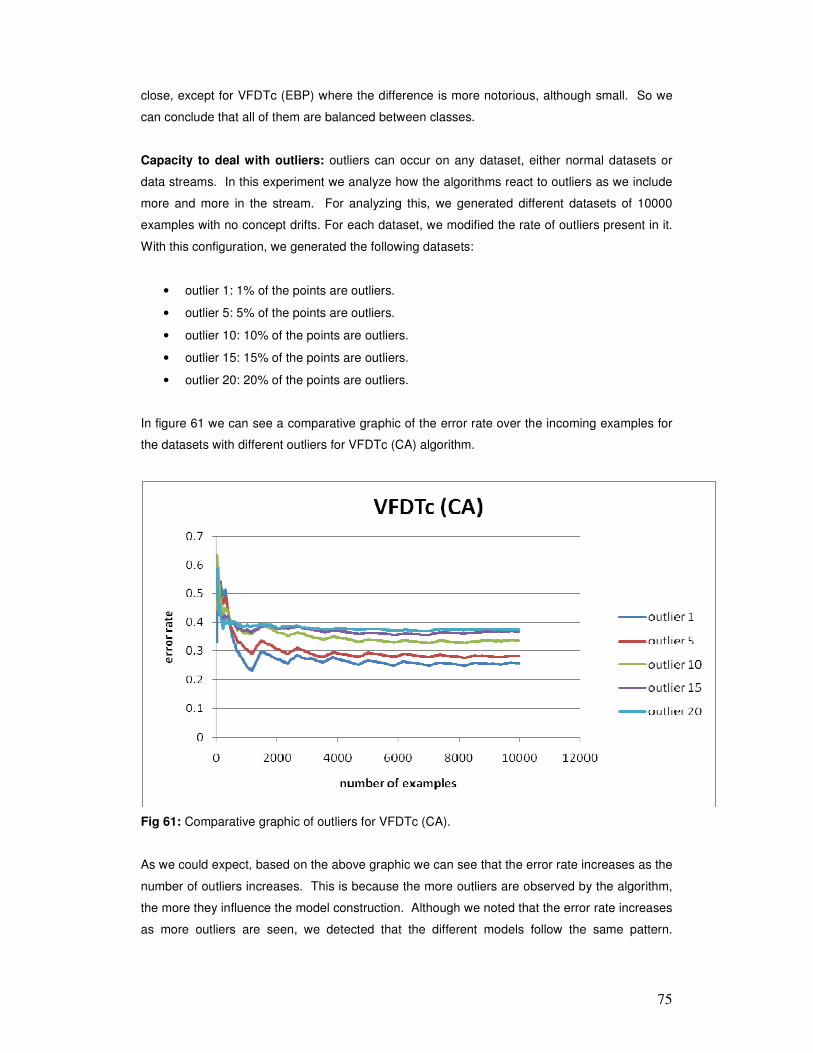
75

close, except for VFDTc (EBP) where the difference is more notorious, although small. So we

can conclude that all of them are balanced between classes.

Capacity to deal with outliers: outliers can occur on any dataset, either normal datasets or

data streams. In this experiment we analyze how the algorithms react to outliers as we include

more and more in the stream. For analyzing this, we generated different datasets of 10000

examples with no concept drifts. For each dataset, we modified the rate of outliers present in it.

With this configuration, we generated the following datasets:

• outlier 1: 1% of the points are outliers.

• outlier 5: 5% of the points are outliers.

• outlier 10: 10% of the points are outliers.

• outlier 15: 15% of the points are outliers.

• outlier 20: 20% of the points are outliers.

In figure 61 we can see a comparative graphic of the error rate over the incoming examples for

the datasets with different outliers for VFDTc (CA) algorithm.

Fig 61: Comparative graphic of outliers for VFDTc (CA).

As we could expect, based on the above graphic we can see that the error rate increases as the

number of outliers increases. This is because the more outliers are observed by the algorithm,

the more they influence the model construction. Although we noted that the error rate increases

as more outliers are seen, we detected that the different models follow the same pattern.

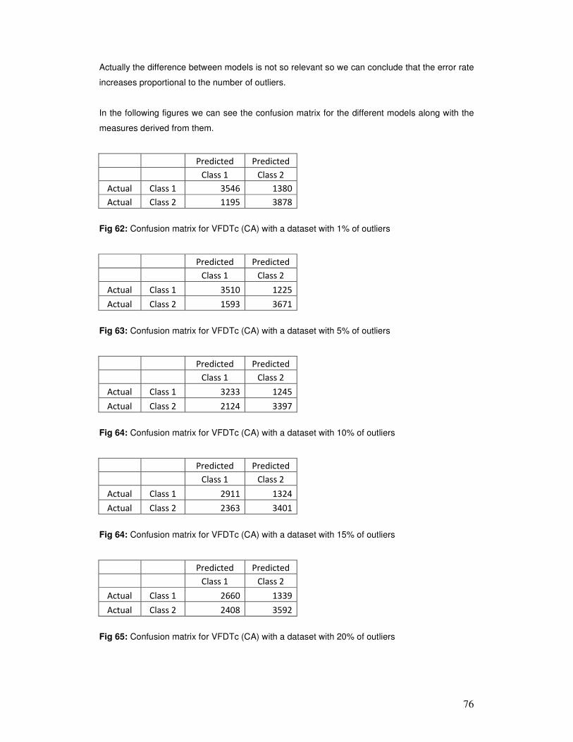
76

Actually the difference between models is not so relevant so we can conclude that the error rate

increases proportional to the number of outliers.

In the following figures we can see the confusion matrix for the different models along with the

measures derived from them.

Predicted Predicted

Class 1 Class 2

Actual Class 1 3546 1380

Actual Class 2 1195 3878

Fig 62: Confusion matrix for VFDTc (CA) with a dataset with 1% of outliers

Predicted Predicted

Class 1 Class 2

Actual Class 1 3510 1225

Actual Class 2 1593 3671

Fig 63: Confusion matrix for VFDTc (CA) with a dataset with 5% of outliers

Predicted Predicted

Class 1 Class 2

Actual Class 1 3233 1245

Actual Class 2 2124 3397

Fig 64: Confusion matrix for VFDTc (CA) with a dataset with 10% of outliers

Predicted Predicted

Class 1 Class 2

Actual Class 1 2911 1324

Actual Class 2 2363 3401

Fig 64: Confusion matrix for VFDTc (CA) with a dataset with 15% of outliers

Predicted Predicted

Class 1 Class 2

Actual Class 1 2660 1339

Actual Class 2 2408 3592

Fig 65: Confusion matrix for VFDTc (CA) with a dataset with 20% of outliers

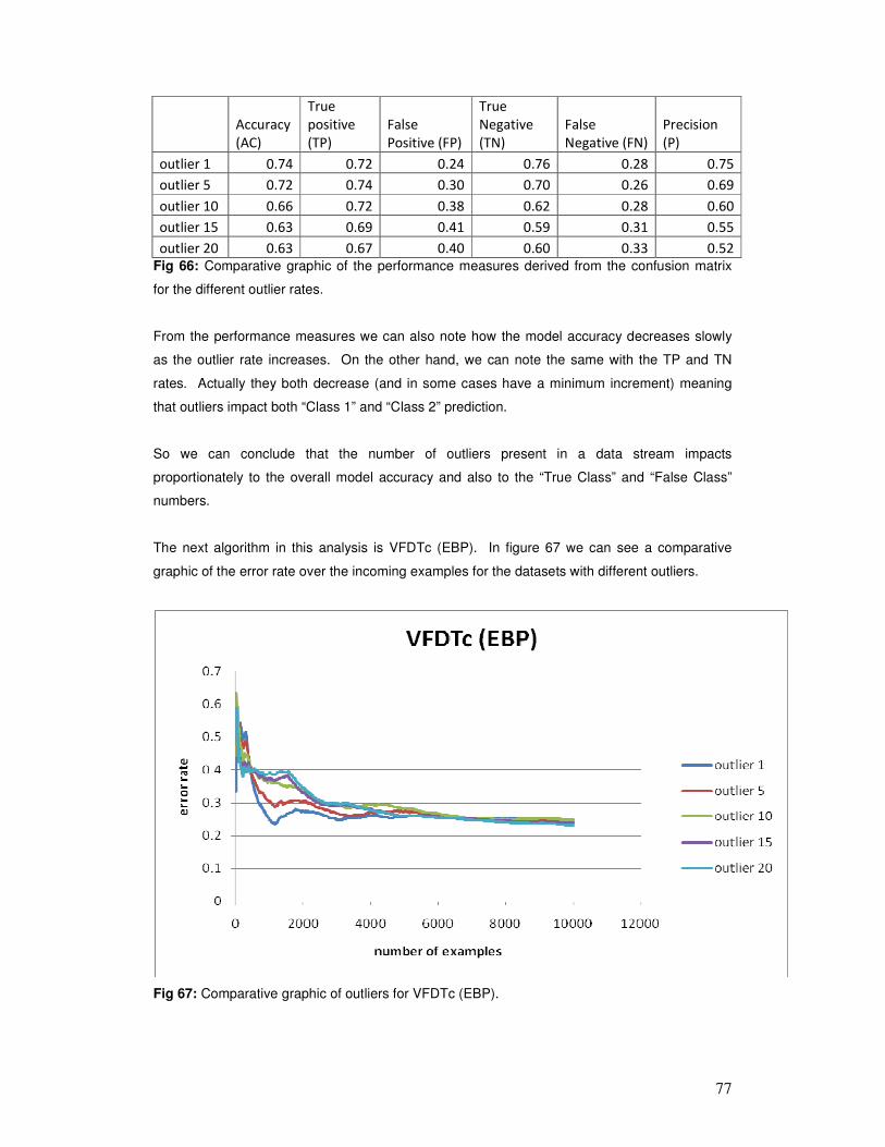
77

Accuracy

(AC)

True

positive

(TP)

False

Positive (FP)

True

Negative

(TN)

False

Negative (FN)

Precision

(P)

outlier 1 0.74 0.72 0.24 0.76 0.28 0.75

outlier 5 0.72 0.74 0.30 0.70 0.26 0.69

outlier 10 0.66 0.72 0.38 0.62 0.28 0.60

outlier 15 0.63 0.69 0.41 0.59 0.31 0.55

outlier 20 0.63 0.67 0.40 0.60 0.33 0.52

Fig 66: Comparative graphic of the performance measures derived from the confusion matrix

for the different outlier rates.

From the performance measures we can also note how the model accuracy decreases slowly

as the outlier rate increases. On the other hand, we can note the same with the TP and TN

rates. Actually they both decrease (and in some cases have a minimum increment) meaning

that outliers impact both “Class 1” and “Class 2” prediction.

So we can conclude that the number of outliers present in a data stream impacts

proportionately to the overall model accuracy and also to the “True Class” and “False Class”

numbers.

The next algorithm in this analysis is VFDTc (EBP). In figure 67 we can see a comparative

graphic of the error rate over the incoming examples for the datasets with different outliers.

Fig 67: Comparative graphic of outliers for VFDTc (EBP).

78

From the above graphic we can note that during the first examples, the error rate increases as

the number of outliers increase. But then, as the new examples start coming we can note how

the different models get stabled and converge to the same error rate (we can note this by

seeing all the lines overlapped). So we can conclude that VFDTc (EBP) is robust to outliers.

This means that the algorithm detects the outliers and treats it correctly without impacting the

overall model.

In the following figures we can see the confusion matrix for different models along with the

measures derived from them.

Predicted Predicted

Class 1 Class 2

Actual Class 1 3772 1154

Actual Class 2 1231 3842

Fig 68: Confusion matrix for VFDTc (EBP) with a dataset with 1% of outliers

Predicted Predicted

Class 1 Class 2

Actual Class 1 3549 1186

Actual Class 2 1288 3976

Fig 69: Confusion matrix for VFDTc (EBP) with a dataset with 5% of outliers

Predicted Predicted

Class 1 Class 2

Actual Class 1 3412 1066

Actual Class 2 1412 4109

Fig 70: Confusion matrix for VFDTc (EBP) with a dataset with 10% of outliers

Predicted Predicted

Class 1 Class 2

Actual Class 1 3098 1137

Actual Class 2 1237 4527

Fig 71: Confusion matrix for VFDTc (EBP) with a dataset with 15% of outliers

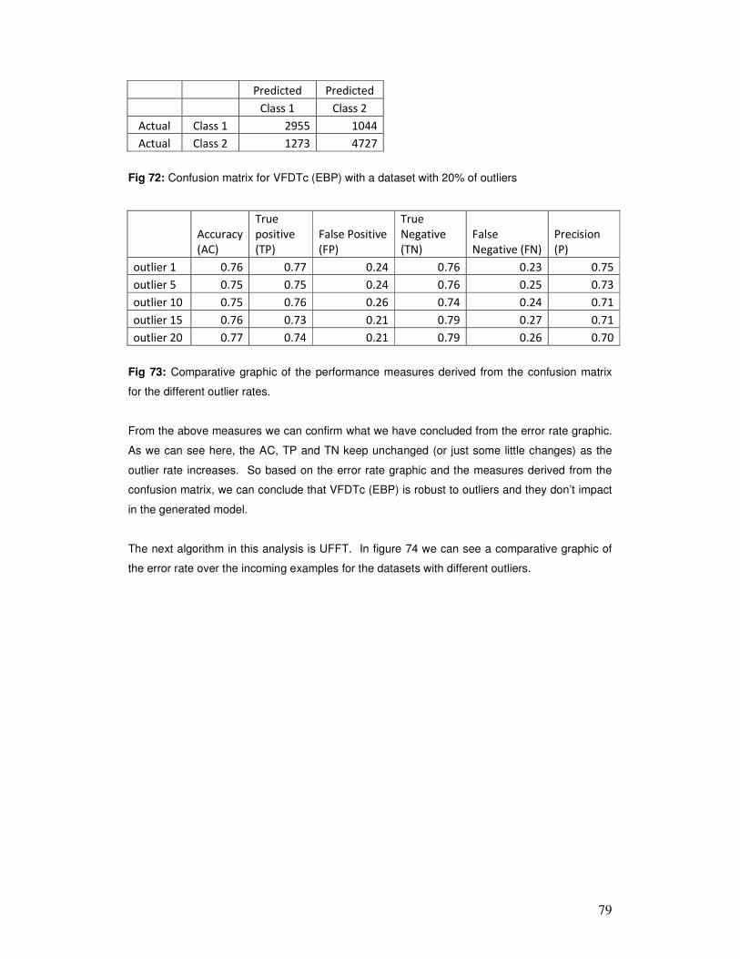
79

Predicted Predicted

Class 1 Class 2

Actual Class 1 2955 1044

Actual Class 2 1273 4727

Fig 72: Confusion matrix for VFDTc (EBP) with a dataset with 20% of outliers

Accuracy

(AC)

True

positive

(TP)

False Positive

(FP)

True

Negative

(TN)

False

Negative (FN)

Precision

(P)

outlier 1 0.76 0.77 0.24 0.76 0.23 0.75

outlier 5 0.75 0.75 0.24 0.76 0.25 0.73

outlier 10 0.75 0.76 0.26 0.74 0.24 0.71

outlier 15 0.76 0.73 0.21 0.79 0.27 0.71

outlier 20 0.77 0.74 0.21 0.79 0.26 0.70

Fig 73: Comparative graphic of the performance measures derived from the confusion matrix

for the different outlier rates.

From the above measures we can confirm what we have concluded from the error rate graphic.

As we can see here, the AC, TP and TN keep unchanged (or just some little changes) as the

outlier rate increases. So based on the error rate graphic and the measures derived from the

confusion matrix, we can conclude that VFDTc (EBP) is robust to outliers and they don’t impact

in the generated model.

The next algorithm in this analysis is UFFT. In figure 74 we can see a comparative graphic of

the error rate over the incoming examples for the datasets with different outliers.

80

Fig 74: Comparative graphic of outliers for UFFT.

Opposite to VFDTc (CA) and VFDTc (EBP), we can note that UFFT is very sensitive to outliers.

Actually, analyzing the graphic we can note 2 groups. One of them consists of the models with

the lowest outlier rates (outlier 1 and outlier 5) where the error stays between 0.1 and 0.2. The

other group consist of the models with the highest outlier rate (outlier 10, outlier 15 and outlier

20) where the error stays between 0.3 and 0.4. So we can note that the error rate increases

abruptly as the number of outliers increases.

In the following figures we can see the confusion matrix for the different models along with the

measures derived from them.

Predicted Predicted

Class 1 Class 2

Actual Class 1 3328 363

Actual Class 2 583 3175

Fig 75: Confusion matrix for UFFT with a dataset with 1% of outliers

Predicted Predicted

Class 1 Class 2

Actual Class 1 2221 242

Actual Class 2 618 2158

Fig 76: Confusion matrix for UFFT with a dataset with 5% of outliers

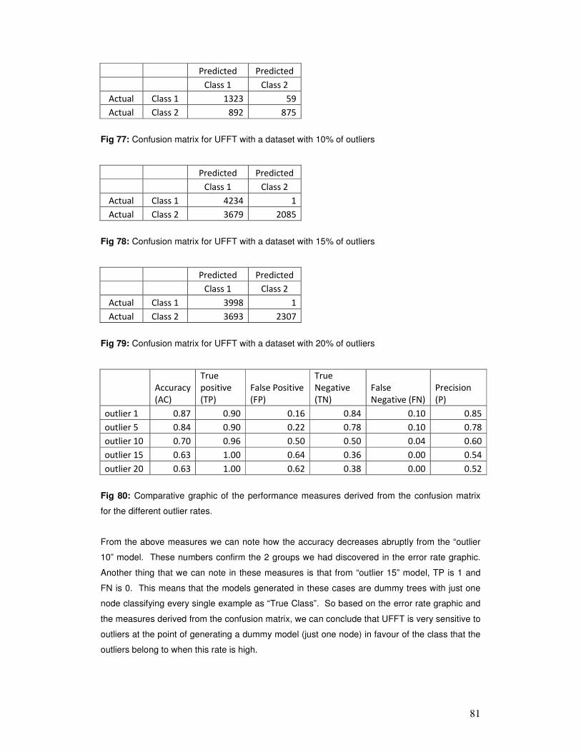
81

Predicted Predicted

Class 1 Class 2

Actual Class 1 1323 59

Actual Class 2 892 875

Fig 77: Confusion matrix for UFFT with a dataset with 10% of outliers

Predicted Predicted

Class 1 Class 2

Actual Class 1 4234 1

Actual Class 2 3679 2085

Fig 78: Confusion matrix for UFFT with a dataset with 15% of outliers

Predicted Predicted

Class 1 Class 2

Actual Class 1 3998 1

Actual Class 2 3693 2307

Fig 79: Confusion matrix for UFFT with a dataset with 20% of outliers

Accuracy

(AC)

True

positive

(TP)

False Positive

(FP)

True

Negative

(TN)

False

Negative (FN)

Precision

(P)

outlier 1 0.87 0.90 0.16 0.84 0.10 0.85

outlier 5 0.84 0.90 0.22 0.78 0.10 0.78

outlier 10 0.70 0.96 0.50 0.50 0.04 0.60

outlier 15 0.63 1.00 0.64 0.36 0.00 0.54

outlier 20 0.63 1.00 0.62 0.38 0.00 0.52

Fig 80: Comparative graphic of the performance measures derived from the confusion matrix

for the different outlier rates.

From the above measures we can note how the accuracy decreases abruptly from the “outlier

10” model. These numbers confirm the 2 groups we had discovered in the error rate graphic.

Another thing that we can note in these measures is that from “outlier 15” model, TP is 1 and

FN is 0. This means that the models generated in these cases are dummy trees with just one

node classifying every single example as “True Class”. So based on the error rate graphic and

the measures derived from the confusion matrix, we can conclude that UFFT is very sensitive to

outliers at the point of generating a dummy model (just one node) in favour of the class that the

outliers belong to when this rate is high.

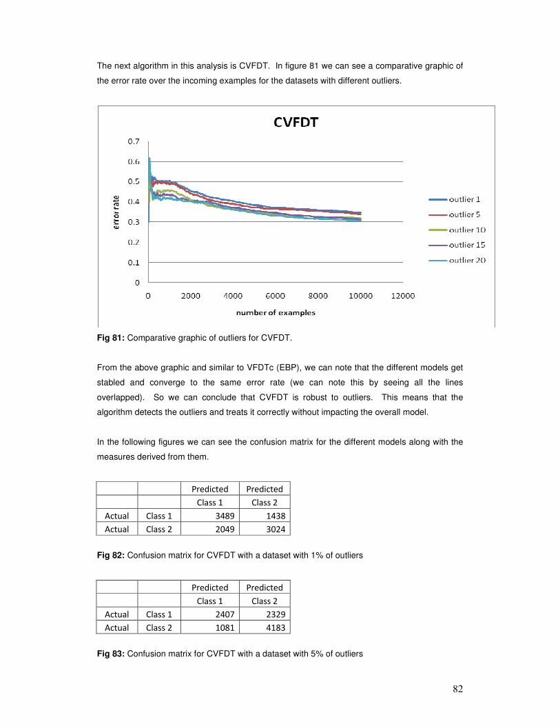
82

The next algorithm in this analysis is CVFDT. In figure 81 we can see a comparative graphic of

the error rate over the incoming examples for the datasets with different outliers.

Fig 81: Comparative graphic of outliers for CVFDT.

From the above graphic and similar to VFDTc (EBP), we can note that the different models get

stabled and converge to the same error rate (we can note this by seeing all the lines

overlapped). So we can conclude that CVFDT is robust to outliers. This means that the

algorithm detects the outliers and treats it correctly without impacting the overall model.

In the following figures we can see the confusion matrix for the different models along with the

measures derived from them.

Predicted Predicted

Class 1 Class 2

Actual Class 1 3489 1438

Actual Class 2 2049 3024

Fig 82: Confusion matrix for CVFDT with a dataset with 1% of outliers

Predicted Predicted

Class 1 Class 2

Actual Class 1 2407 2329

Actual Class 2 1081 4183

Fig 83: Confusion matrix for CVFDT with a dataset with 5% of outliers

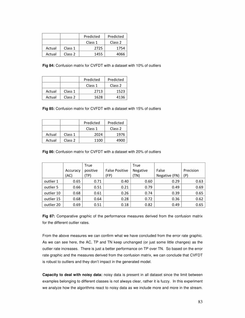
83

Predicted Predicted

Class 1 Class 2

Actual Class 1 2725 1754

Actual Class 2 1455 4066

Fig 84: Confusion matrix for CVFDT with a dataset with 10% of outliers

Predicted Predicted

Class 1 Class 2

Actual Class 1 2713 1523

Actual Class 2 1628 4136

Fig 85: Confusion matrix for CVFDT with a dataset with 15% of outliers

Predicted Predicted

Class 1 Class 2

Actual Class 1 2024 1976

Actual Class 2 1100 4900

Fig 86: Confusion matrix for CVFDT with a dataset with 20% of outliers

Accuracy

(AC)

True

positive

(TP)

False Positive

(FP)

True

Negative

(TN)

False

Negative (FN)

Precision

(P)

outlier 1 0.65 0.71 0.40 0.60 0.29 0.63

outlier 5 0.66 0.51 0.21 0.79 0.49 0.69

outlier 10 0.68 0.61 0.26 0.74 0.39 0.65

outlier 15 0.68 0.64 0.28 0.72 0.36 0.62

outlier 20 0.69 0.51 0.18 0.82 0.49 0.65

Fig 87: Comparative graphic of the performance measures derived from the confusion matrix

for the different outlier rates.

From the above measures we can confirm what we have concluded from the error rate graphic.

As we can see here, the AC, TP and TN keep unchanged (or just some little changes) as the

outlier rate increases. There is just a better performance on TP over TN. So based on the error

rate graphic and the measures derived from the confusion matrix, we can conclude that CVFDT

is robust to outliers and they don’t impact in the generated model.

Capacity to deal with noisy data: noisy data is present in all dataset since the limit between

examples belonging to different classes is not always clear, rather it is fuzzy. In this experiment

we analyze how the algorithms react to noisy data as we include more and more in the stream.

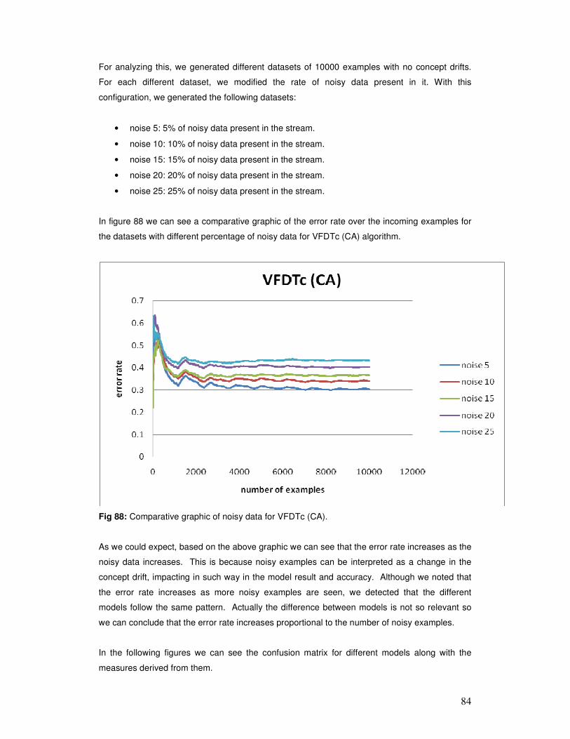
84

For analyzing this, we generated different datasets of 10000 examples with no concept drifts.

For each different dataset, we modified the rate of noisy data present in it. With this

configuration, we generated the following datasets:

• noise 5: 5% of noisy data present in the stream.

• noise 10: 10% of noisy data present in the stream.

• noise 15: 15% of noisy data present in the stream.

• noise 20: 20% of noisy data present in the stream.

• noise 25: 25% of noisy data present in the stream.

In figure 88 we can see a comparative graphic of the error rate over the incoming examples for

the datasets with different percentage of noisy data for VFDTc (CA) algorithm.

Fig 88: Comparative graphic of noisy data for VFDTc (CA).

As we could expect, based on the above graphic we can see that the error rate increases as the

noisy data increases. This is because noisy examples can be interpreted as a change in the

concept drift, impacting in such way in the model result and accuracy. Although we noted that

the error rate increases as more noisy examples are seen, we detected that the different

models follow the same pattern. Actually the difference between models is not so relevant so

we can conclude that the error rate increases proportional to the number of noisy examples.

In the following figures we can see the confusion matrix for different models along with the

measures derived from them.

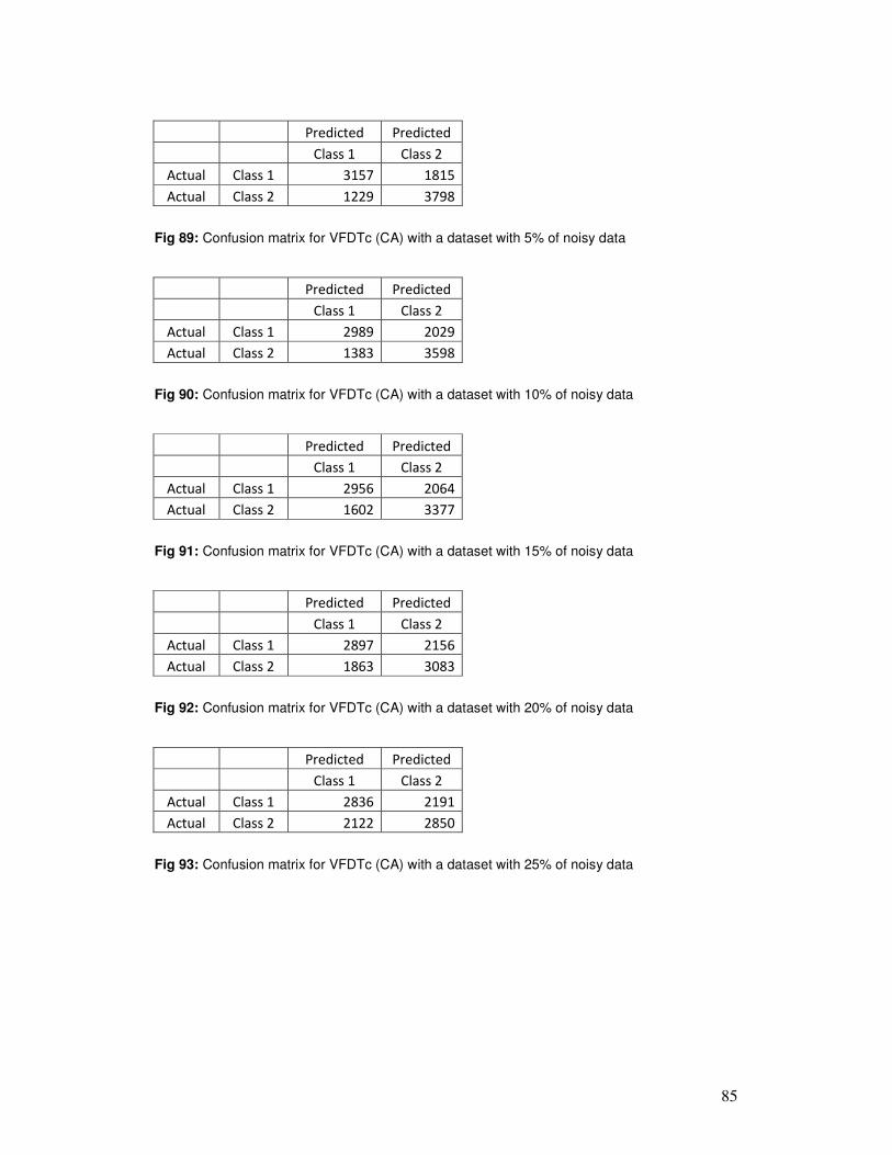
85

Predicted Predicted

Class 1 Class 2

Actual Class 1 3157 1815

Actual Class 2 1229 3798

Fig 89: Confusion matrix for VFDTc (CA) with a dataset with 5% of noisy data

Predicted Predicted

Class 1 Class 2

Actual Class 1 2989 2029

Actual Class 2 1383 3598

Fig 90: Confusion matrix for VFDTc (CA) with a dataset with 10% of noisy data

Predicted Predicted

Class 1 Class 2

Actual Class 1 2956 2064

Actual Class 2 1602 3377

Fig 91: Confusion matrix for VFDTc (CA) with a dataset with 15% of noisy data

Predicted Predicted

Class 1 Class 2

Actual Class 1 2897 2156

Actual Class 2 1863 3083

Fig 92: Confusion matrix for VFDTc (CA) with a dataset with 20% of noisy data

Predicted Predicted

Class 1 Class 2

Actual Class 1 2836 2191

Actual Class 2 2122 2850

Fig 93: Confusion matrix for VFDTc (CA) with a dataset with 25% of noisy data

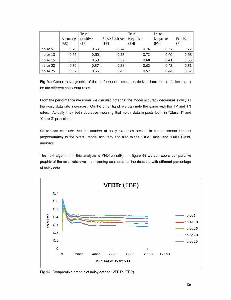
86

Accuracy

(AC)

True

positive

(TP)

False Positive

(FP)

True

Negative

(TN)

False

Negative

(FN)

Precision

(P)

noise 5 0.70 0.63 0.24 0.76 0.37 0.72

noise 10 0.66 0.60 0.28 0.72 0.40 0.68

noise 15 0.63 0.59 0.32 0.68 0.41 0.65

noise 20 0.60 0.57 0.38 0.62 0.43 0.61

noise 25 0.57 0.56 0.43 0.57 0.44 0.57

Fig 94: Comparative graphic of the performance measures derived from the confusion matrix

for the different noisy data rates.

From the performance measures we can also note that the model accuracy decreases slowly as

the noisy data rate increases. On the other hand, we can note the same with the TP and TN

rates. Actually they both decrease meaning that noisy data impacts both in “Class 1” and

“Class 2” prediction.

So we can conclude that the number of noisy examples present in a data stream impacts

proportionately to the overall model accuracy and also to the “True Class” and “False Class”

numbers.

The next algorithm in this analysis is VFDTc (EBP). In figure 95 we can see a comparative

graphic of the error rate over the incoming examples for the datasets with different percentage

of noisy data.

Fig 95: Comparative graphic of noisy data for VFDTc (EBP).

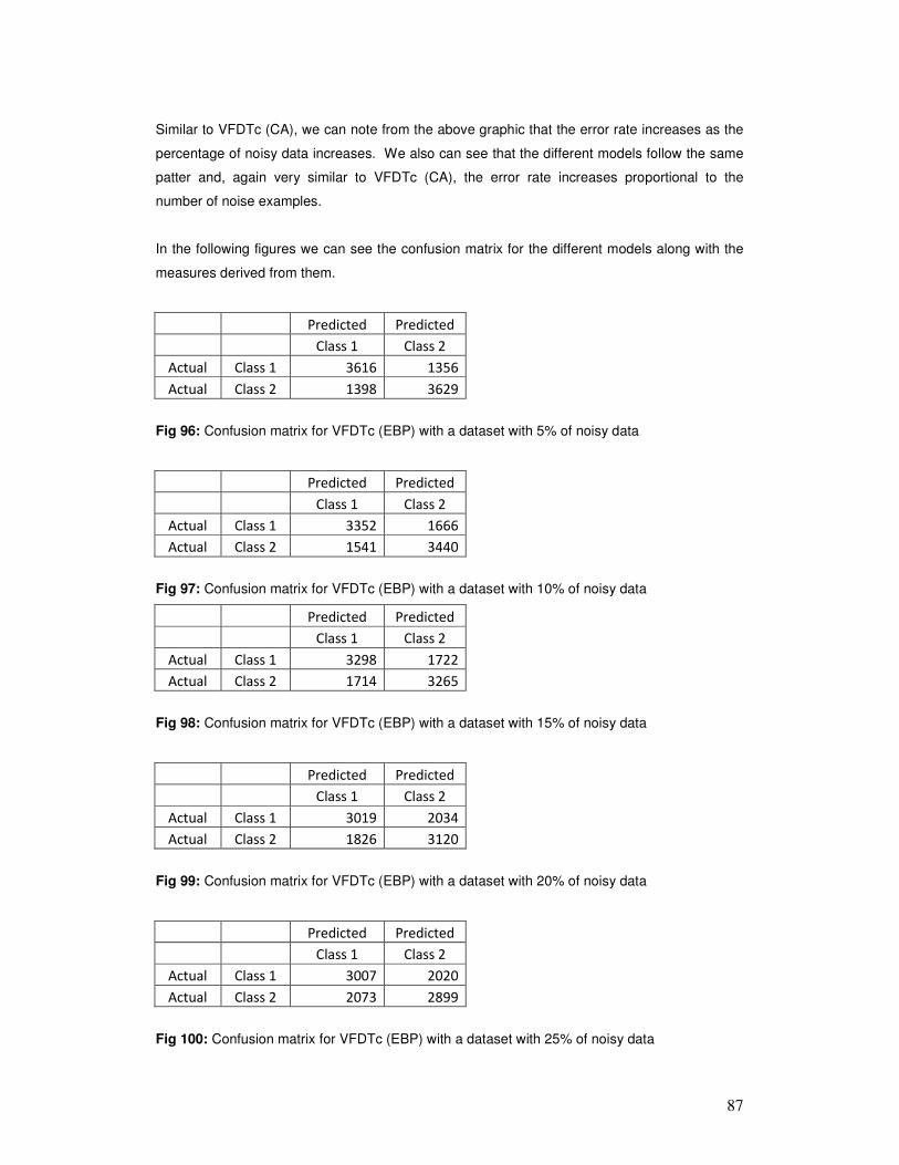
87

Similar to VFDTc (CA), we can note from the above graphic that the error rate increases as the

percentage of noisy data increases. We also can see that the different models follow the same

patter and, again very similar to VFDTc (CA), the error rate increases proportional to the

number of noise examples.

In the following figures we can see the confusion matrix for the different models along with the

measures derived from them.

Predicted Predicted

Class 1 Class 2

Actual Class 1 3616 1356

Actual Class 2 1398 3629

Fig 96: Confusion matrix for VFDTc (EBP) with a dataset with 5% of noisy data

Predicted Predicted

Class 1 Class 2

Actual Class 1 3352 1666

Actual Class 2 1541 3440

Fig 97: Confusion matrix for VFDTc (EBP) with a dataset with 10% of noisy data

Predicted Predicted

Class 1 Class 2

Actual Class 1 3298 1722

Actual Class 2 1714 3265

Fig 98: Confusion matrix for VFDTc (EBP) with a dataset with 15% of noisy data

Predicted Predicted

Class 1 Class 2

Actual Class 1 3019 2034

Actual Class 2 1826 3120

Fig 99: Confusion matrix for VFDTc (EBP) with a dataset with 20% of noisy data

Predicted Predicted

Class 1 Class 2

Actual Class 1 3007 2020

Actual Class 2 2073 2899

Fig 100: Confusion matrix for VFDTc (EBP) with a dataset with 25% of noisy data

88

Accuracy

(AC)

True

positive

(TP)

False Positive

(FP)

True

Negative

(TN)

False

Negative

(FN)

Precision

(P)

noise 5 0.72 0.73 0.28 0.72 0.27 0.72

noise 10 0.68 0.67 0.31 0.69 0.33 0.69

noise 15 0.66 0.66 0.34 0.66 0.34 0.66

noise 20 0.61 0.60 0.37 0.63 0.40 0.62

noise 25 0.59 0.60 0.42 0.58 0.40 0.59

Fig 101: Comparative graphic of the performance measures derived from the confusion matrix

for the different noisy data rates.

As we noted in the error rate graphic for VFDTc (EBP) where we mentioned that the error rate

behaviour was very similar to VFDTc (CA), from the performance measure we can also note

these similarities. That is, we can note that the model accuracy decreases slowly as the rate of

noisy data increases. Also, we can note the same behaviour with TP and TN rates.

So as we concluded for VFDTc (CA), we can also mention for VFDTc (EBP) that the number of

noisy examples present in a data stream impacts proportionately to the overall model accuracy

and also to the “True Class” and “False Class” numbers.

The next algorithm in this analysis is UFFT. In figure 102 we can see a comparative graphic of

the error rate over the incoming examples for the datasets with different percentage of noisy

data.

Fig 102: Comparative graphic of noisy data for UFFT.

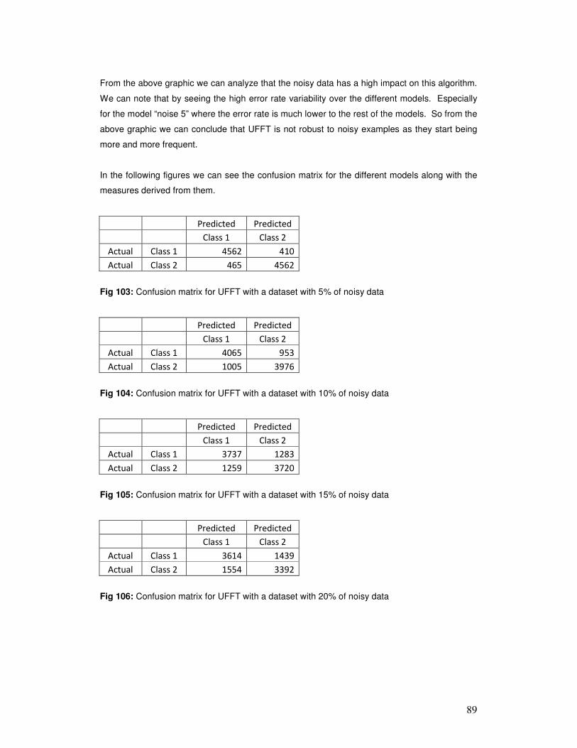
89

From the above graphic we can analyze that the noisy data has a high impact on this algorithm.

We can note that by seeing the high error rate variability over the different models. Especially

for the model “noise 5” where the error rate is much lower to the rest of the models. So from the

above graphic we can conclude that UFFT is not robust to noisy examples as they start being

more and more frequent.

In the following figures we can see the confusion matrix for the different models along with the

measures derived from them.

Predicted Predicted

Class 1 Class 2

Actual Class 1 4562 410

Actual Class 2 465 4562

Fig 103: Confusion matrix for UFFT with a dataset with 5% of noisy data

Predicted Predicted

Class 1 Class 2

Actual Class 1 4065 953

Actual Class 2 1005 3976

Fig 104: Confusion matrix for UFFT with a dataset with 10% of noisy data

Predicted Predicted

Class 1 Class 2

Actual Class 1 3737 1283

Actual Class 2 1259 3720

Fig 105: Confusion matrix for UFFT with a dataset with 15% of noisy data

Predicted Predicted

Class 1 Class 2

Actual Class 1 3614 1439

Actual Class 2 1554 3392

Fig 106: Confusion matrix for UFFT with a dataset with 20% of noisy data

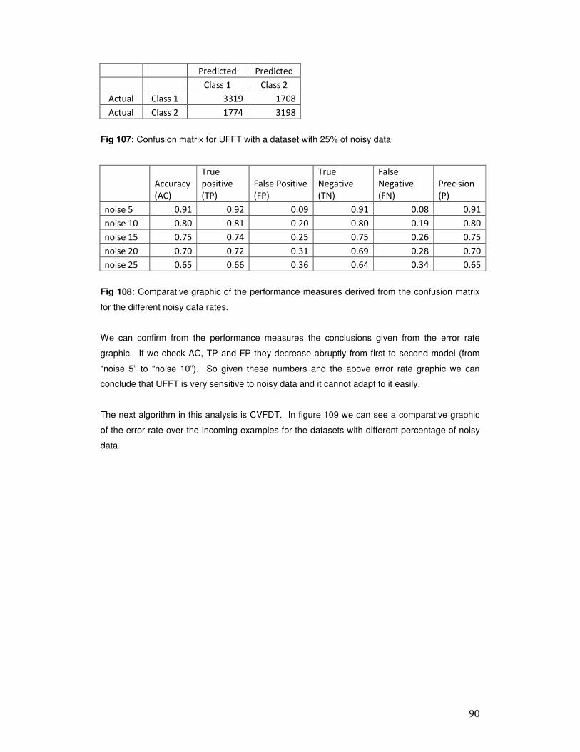
90

Predicted Predicted

Class 1 Class 2

Actual Class 1 3319 1708

Actual Class 2 1774 3198

Fig 107: Confusion matrix for UFFT with a dataset with 25% of noisy data

Accuracy

(AC)

True

positive

(TP)

False Positive

(FP)

True

Negative

(TN)

False

Negative

(FN)

Precision

(P)

noise 5 0.91 0.92 0.09 0.91 0.08 0.91

noise 10 0.80 0.81 0.20 0.80 0.19 0.80

noise 15 0.75 0.74 0.25 0.75 0.26 0.75

noise 20 0.70 0.72 0.31 0.69 0.28 0.70

noise 25 0.65 0.66 0.36 0.64 0.34 0.65

Fig 108: Comparative graphic of the performance measures derived from the confusion matrix

for the different noisy data rates.

We can confirm from the performance measures the conclusions given from the error rate

graphic. If we check AC, TP and FP they decrease abruptly from first to second model (from

“noise 5” to “noise 10”). So given these numbers and the above error rate graphic we can

conclude that UFFT is very sensitive to noisy data and it cannot adapt to it easily.

The next algorithm in this analysis is CVFDT. In figure 109 we can see a comparative graphic

of the error rate over the incoming examples for the datasets with different percentage of noisy

data.

91

Fig 109: Comparative graphic of noisy data for CVFDT.

As we can note in the above graphic, all the lines are overlapped, meaning that CVFDT

performs in the same way regardless of the percentage of noise in the data. This also means

that the algorithm is very robust to noisy data, even more robust than VFDTc (CA) and VFDTc

(EBP) since the difference between models is minimal. So based on this graphic we can

conclude that CVFDT is very robust to noisy data.

In the following figures we can see the confusion matrix for the different models along with the

measures derived from them.

Predicted Predicted

Class 1 Class 2

Actual Class 1 3490 1483

Actual Class 2 2177 2850

Fig 110: Confusion matrix for CVFDT with a dataset with 5% of noisy data

Predicted Predicted

Class 1 Class 2

Actual Class 1 3429 1590

Actual Class 2 2224 2757

Fig 111: Confusion matrix for CVFDT with a dataset with 10% of noisy data

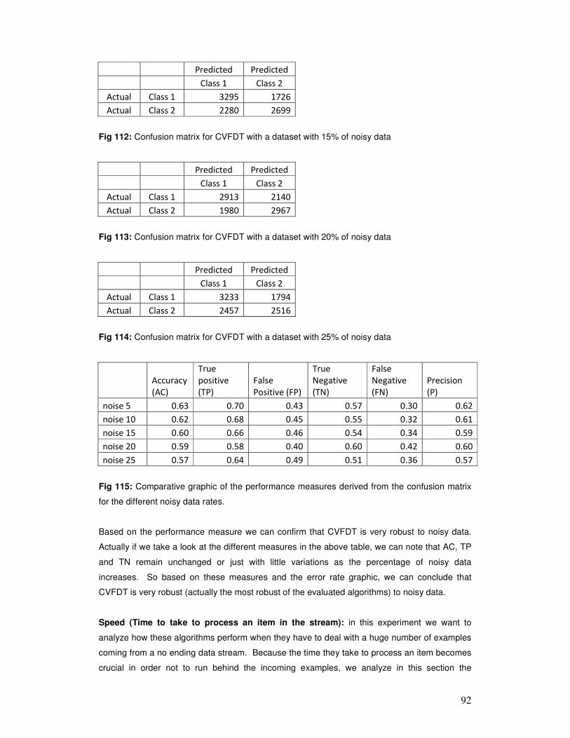
92

Predicted Predicted

Class 1 Class 2

Actual Class 1 3295 1726

Actual Class 2 2280 2699

Fig 112: Confusion matrix for CVFDT with a dataset with 15% of noisy data

Predicted Predicted

Class 1 Class 2

Actual Class 1 2913 2140

Actual Class 2 1980 2967

Fig 113: Confusion matrix for CVFDT with a dataset with 20% of noisy data

Predicted Predicted

Class 1 Class 2

Actual Class 1 3233 1794

Actual Class 2 2457 2516

Fig 114: Confusion matrix for CVFDT with a dataset with 25% of noisy data

Accuracy

(AC)

True

positive

(TP)

False

Positive (FP)

True

Negative

(TN)

False

Negative

(FN)

Precision

(P)

noise 5 0.63 0.70 0.43 0.57 0.30 0.62

noise 10 0.62 0.68 0.45 0.55 0.32 0.61

noise 15 0.60 0.66 0.46 0.54 0.34 0.59

noise 20 0.59 0.58 0.40 0.60 0.42 0.60

noise 25 0.57 0.64 0.49 0.51 0.36 0.57

Fig 115: Comparative graphic of the performance measures derived from the confusion matrix

for the different noisy data rates.

Based on the performance measure we can confirm that CVFDT is very robust to noisy data.

Actually if we take a look at the different measures in the above table, we can note that AC, TP

and TN remain unchanged or just with little variations as the percentage of noisy data

increases. So based on these measures and the error rate graphic, we can conclude that

CVFDT is very robust (actually the most robust of the evaluated algorithms) to noisy data.

Speed (Time to take to process an item in the stream): in this experiment we want to

analyze how these algorithms perform when they have to deal with a huge number of examples

coming from a no ending data stream. Because the time they take to process an item becomes

crucial in order not to run behind the incoming examples, we analyze in this section the

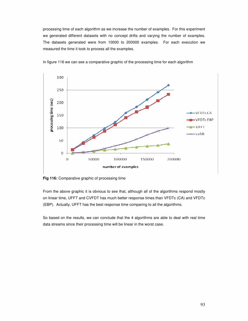
93

processing time of each algorithm as we increase the number of examples. For this experiment

we generated different datasets with no concept drifts and varying the number of examples.

The datasets generated were from 10000 to 200000 examples. For each execution we

measured the time it took to process all the examples.

In figure 116 we can see a comparative graphic of the processing time for each algorithm

Fig 116: Comparative graphic of processing time

From the above graphic it is obvious to see that, although all of the algorithms respond mostly

on linear time, UFFT and CVFDT has much better response times than VFDTc (CA) and VFDTc

(EBP). Actually, UFFT has the best response time comparing to all the algorithms.

So based on the results, we can conclude that the 4 algorithms are able to deal with real time

data streams since their processing time will be linear in the worst case.

94

7 Conclusions and Future work

We have discussed in this thesis how more and more companies and organizations have to

deal with huge amount of data, in some cases generating million of registers per day. This

scenario and the fact that the data can be generated very fast give us a new and challenging

way of developing and applying Data Mining algorithms. In this new scenario, the data cannot

be reviewed or processed more than once, because if we did so, we would not be able to

process all the incoming items in such a fast way. On the other hand, given that the algorithms

cannot see all the items to be processed, we have to develop them having in mind that the

training phase can never end. Basically what we are doing is training algorithms from data

streams. One of the challenges associated with this situation is how to deal with the order in

which the items arrive to the algorithm. In contrast to off-line learning where algorithms are

developed assuming that all the data is available before the training and there is no order, in on-

line learning the items are time-ordered and the distribution that generates them can vary over

time.

The changes in the data distribution are another challenging scenario that data stream mining

has to deal with. This phenomenon is known as concept drift. We highlighted that there has

been a lot of previous work trying to make these algorithms detect and adapt to concept drifts

so they can keep their model up to date with the underlying data distribution. Some of these

approaches are: instance selection (basically using a fixed or dynamic window), instance

weighting (dropping all the instances that weight less than a threshold) and ensemble learning

(using and ensemble of classification algorithms).

Another point that it is worth to highlight here is to mention VFDT as one of the first data stream

mining algorithms developed. Although this algorithm is not able to detect concept drift, it uses

an interesting statistical measure (the Hoeffding bound) to determine the number of examples

needed at each tree node to make statically valid assumptions like it had all the data available.

Regarding the benchmarking analysis we developed the experiment for 3 of the most important

algorithms available for mining data streams: UFFT, VFDTc and CVFDT. The experiment was

about comparing the behavior and performance of the generated models taking into account 10

different characteristics that any classification algorithm applied to data streams has to deal with

and that is explained in section 4. For all the experiments, we generated different datasets

using the moving hyper plane algorithm explained in section 5.

Regarding the result of the experiments we can note that UFFT performed better for all the

experiments since its error rate for all of them keeps lower than the error rate of the other

algorithms. So if we are interested in the overall performance of the model, then UFFT could be

the option no matter the characteristics of the data stream. But, if we are more interested in a

95

model with the capacity of adapting better to certain circumstances (like concept drift, virtual

concept drift, etc), then our previous selection might change. If we are more focused on short

term predictions, UFFT should be our choice as its error rate goes down very fast and then it

increases while CVFDT is more suitable for long term solution as the error rate decreases

smoothly but continuously. Then we detected that none of the algorithms are impacted by

virtual concept drift or recurring concept drift, so we don’t have to worry about these

characteristics when we have to select an algorithm. If we have to work with data streams and

we know it has different level of concept drift (from gradual to sudden) then we shouldn’t use

VFDTc (CA) since it is very sensitive to these changes. On the other hand, if the data stream

has very frequent concept drift, then VFDTc (CA) or UFFT might be not suitable for this scenario

since they are very sensitive to these changes. For data streams having outliers, the most

suitable algorithms should be VFDTc (EBP) and CVFDT since they are robust to the increment

of outliers in the long term. On the other hand, if we have data streams with noisy data, we

should select CVFDT as it is very robust to this type of data. Finally if we want fast algorithms,

based on this research, CVFDT and UFFT are the fastest.

As for future work, we will need to do some research on clustering algorithms applied to data

streams. That is, algorithms that can adapt and change their cluster dynamically as new data

come in the stream. Also these algorithms need to be able to detect concept drift and change

their cluster accordingly and also update the statistics of the cluster in an incremental way in

order to process each item faster. On the other hand, all the classification algorithms evaluated

here were applied to structured datasets. Another subject of researching is classification

algorithms applied to data streams of unstructured datasets like text, images, etc. In this case,

in addition to the challenges topics discussed in the thesis we will have to figure out how to

analyse and process unstructured data fast enough for dealing with data streams.

96

8 References

[1] Jeffrey C.Schlimmer, Richard H.Granger, Jr. Incremental Learning from Noisy Data. Machine

Learning 1:317-354. 1986

[2] Ivan Koychev. Gradual Forgetting for Adaptation to Concept Drift. Sankt Augustin,

Germany. 2000.

[3] Ying Yang, Xindong Wu and Xingquan Zhu. Combining Proactive and Reactive Predictions

for Data Streams. KDD’05, Chicago, Illinois, USA. August 21–24, 2005.

[4] Michael Harries, Claude Sammut. Extracting Hidden Context. School of Computer Science

and Engineering. The University of New South Wales, Sydney, Australia. November 1997.

[5] Mark Last. Online Classification of Nonstationary Data Streams. Intelligent Data Analysis,

Vol. 6, No. 2, pp. 129-147. 2002.

[6] Ricard Gavaldà. Data Mining on Time-Varying Data Streams using Sequential Sampling.

Universitat Politecnica de Catalunya (UPC), Spain. August 2005.

[7] Joao Gama, Ricardo Fernandes, Ricardo Rocha. Decision Trees for Mining Data Streams.

Intelligent Data Analysis, Volume 10, Issue 1, Pages 23-45. 2006.

[8] Pedro Domingos, Geoff Hulten. Catching Up with the Data: Research Issues in Mining Data

Streams. Workshop on Research Issues in Data Mining and Knowledge Discovery. Santa

Barbara, CA. 2001.

[9] Alexey Tsymbal. The problem of concept drift: definitions and related work. Department of

Computer Science. Trinity College Dublin, Ireland. April 29, 2004

[10] Pedro Domingos, Geoff Hulten. A general Framework for Mining Massive Data Streams.

Journal of Computational & Graphical Statistics. Volume 12, Number 4, pp. 945-949(5), 1

December 2003.

[11] Francisco J. Ferrer-Troyano, Jesús S. Aguilar-Ruiz. Minería de Data Streams: Conceptos y

Principales Técnicas. Universidad de Sevilla. 2005.

[12] G. Dong, J. Pei, J. Han, H. Wang, Lask V.S. Lakshmanan, P. S. Yu. Online Mining of

Changes from Data Streams: Research Problems and Preliminary Results. ACM SIGMOD

MPDS ’03, San Diego, CA, USA. 2002.

[13] Pedro Domingos, Geoff Hulten. Mining high-Speed Data Streams. In: Proc. of The 6th

ACM SIGKDD Int. Conf. on Knowledge Discovery and Data Mining - KDD'00, ACM Press 71-

80. 2000

[14] Michalski, R., Larson, J. Incremental generation of VL1 hypotheses: The underlying

methodology and the description of the program AQ11. Technical Report UIUCDCS-F-83-905,

Department of Computer Science, University of Illinois, Urbana-Champaign. 1983.

[15] Reinke, R., Michalski, R. Incremental learning of concept descriptions: A method and

experimental results. Machine Intelligence 11 263-288. 1986

[16] Schlimmer, J., Granger, R. Beyond incremental processing: Tracking concept drift. In:

Proc. of the 5th National Conf. on Artificial Intelligence, AAAI Press, Menlo Park, CA 502-507.

1986.

97

[17] Gerhard Widmer, Miroslav Kubat. Learning in the Presence of Concept Drift and Hidden

Contexts. Machine Learning, 23, 69-101. 1996.

[18] Marcus A. Maloof, Ryszard S. Michalski. AQ-PM: A System for Partial Memory Learning.

Intelligent Information Systems VIII. Proceedings of the Workshop held in Ustron, Poland, pp.

70-79. June 14-18 1999.

[19] Maloof, M. Incremental rule learning with partial instance memory for changing concepts.

In: Proc. of the Int. Joint Conf. on Neural Networks, IEEE Press, 2764-2769. 2003.

[20] Maloof, M., Michalski, R.: Incremental learning with partial instance memory. Artificial

Intelligence 154, 95-126. 2004.

[21] Joao Gama, Pedro Medas. Learning Decision Trees from Dynamic Data Streams. Journal

of Universal Computer Science, vol. 11 no. 8. 2005.

[22] Geoff Hulten, Laurie Spencer, Pedro Domingos. Mining Time-Changing Data Streams. In:

Proc. of The 7th ACM SIGKDD Int. Conf. on Knowledge Discovery and Data Mining - KDD'01,

ACM Press ,97-106. 2001.

[23] Mihai M. Lazarescu, Svetha Venkatesh, Hung H. Bui. Using Multiple Windows to Track

Concept Drift. Faculty of Computer Science, Curtin University. January 16, 2003.

[24] Sofus Macskassy. A Comparison of Two On-line Algorithms that Adapt to Concept Drift.

Department of Computer Science, Rutgers University. 1998.

[25] Haixun Wang, Wei Fan, Philip S. Yu, Jiawei Han. Mining Concept-Drifting Data Streams

using Ensemble Classifiers. Dept. of Computer Science, Univ. of Illinois, Urbana. 2002.

[26] Lior Cohen, Gil Avrahami, Mark Last. Incremental Info-Fuzzy Algorithm for Real Time Data

Mining of Non-Stationary Data Streams. TDM Workshop, Brighton UK. 2004.

[27] M. R. Henzinger, P. Raghavan, S. Rajagopalan. Computing on data streams. SRC

Technical Note, 1998-011. May 26, 1998.

[28] Lior Cohen, Gil Avrahami, Mark Last, Abraham Kandel, Oscar Kipersztok. Incremental

Classification of Nonstationary Data Streams. Proceedings of the Second International

Workshop on Knowledge Discovery in Data Streams, pp. 117-124, Porto, Portugal. October 7,

2005.

[29] W. Hoeffding. Probability inequalities for sums of bounded random variables. Journal of

the American Statistical Association, 58:13-30. 1963.

[30] http://www2.cs.uregina.ca/~dbd/cs831/notes/confusion_matrix/confusion_matrix.html

[31] http://kdd.ics.uci.edu/databases/kddcup99/task.html

[32] http://sourceforge.net/projects/moa-datastream/

[33] Quinlan, J. R. C4.5: Programs for Machine Learning. Morgan Kaufmann Publisher. 1993.