european journal of mechanics a/solids - stanford...

lable at ScienceDirect

European Journal of Mechanics A/Solids 48 (2014) 112e128

Contents lists avai

European Journal of Mechanics A/Solids

journal homepage: www.elsevier .com/locate/ejmsol

Modeling and simulation of viscous electro-active polymers

Franziska Vogel a, Serdar Göktepe b, Paul Steinmann a, Ellen Kuhl c,*aChair of Applied Mechanics, Friedrich-Alexander Universität Erlangen-Nürnberg (FAU), Egerlandstr. 5, 91058 Erlangen, GermanybDepartment of Civil Engineering, Middle East Technical University, 06800 Ankara, TurkeycDepartment of Mechanical Engineering, Stanford University, 496 Lomita Mall, Stanford, CA 94305-4040, USA

a r t i c l e i n f o

Article history:Received 8 October 2013Accepted 5 February 2014Available online 12 March 2014

Keywords:ElectroactivityElectrostaticsElectroelasticityViscoelasticity

* Corresponding author.E-mail address: [email protected] (E. Kuhl).

http://dx.doi.org/10.1016/j.euromechsol.2014.02.0010997-7538/� 2014 Elsevier Masson SAS. All rights re

a b s t r a c t

Electro-active materials are capable of undergoing large deformation when stimulated by an electricfield. They can be divided into electronic and ionic electro-active polymers (EAPs) depending on theiractuation mechanism based on their composition. We consider electronic EAPs, for which attractiveCoulomb forces or local re-orientation of polar groups cause a bulk deformation. Many of these materialsexhibit pronounced visco-elastic behavior. Here we show the development and implementation of aconstitutive model, which captures the influence of the electric field on the visco-elastic response withina geometrically non-linear finite element framework. The electric field affects not only the equilibriumpart of the strain energy function, but also the viscous part. To adopt the familiar additive split of thestrain from the small strain setting, we formulate the governing equations in the logarithmic strain spaceand additively decompose the logarithmic strain into elastic and viscous parts. We show that theincorporation of the electric field in the viscous response significantly alters the relaxation and hysteresisbehavior of the model. Our parametric study demonstrates that the model is sensitive to the choice of theelectro-viscous coupling parameters. We simulate several actuator structures to illustrate the perfor-mance of the method in typical relaxation and creep scenarios. Our model could serve as a design tool formicro-electro-mechanical systems, microfluidic devices, and stimuli-responsive gels such as artificialskin, tactile displays, or artificial muscle.

� 2014 Elsevier Masson SAS. All rights reserved.

1. Introduction

The past two decades have seen an increasingly growing interestin smart materials that change their shape and their mechanicalbehavior in response to external non-mechanical stimuli. Promi-nent representatives of smart materials are electro-active polymers(EAPs), which react to the excitation by an electric field with a bulkdeformation and a change in their material behavior. For goodreasons, EAPs became popular as artificial muscles (Pelrine et al.,1998; Bar-Cohen, 2002, 2004) since they outperform classical ac-tuators such as electro-magnetic motors, pneumatic systems, pie-zoelectrics or shapememory alloys within small-scale technologiesin many ways (Pelrine et al., 2000a; O’Halloran et al., 2008; Brochuand Pei, 2010). Whenever low weight, production cost, operationfrequency, fast response time or little available space are limitingfactors, EAPs find their application within tunable and adaptivedevices for a broad range of industries (Pelrine et al., 2000b, 2000a).

served.

Due to their flexibility in shape, EAPs have become an attractivedesign element in robotics, optics, acoustics and biomimetics(Pelrine et al., 1998, 2000b; Spencer, 1971) in a variety of actuatorgeometries (O’Halloran et al., 2008).

Depending on their actuation mechanism, EAPs can be dividedinto ionic and electronic electro-active polymers. Based on theirdistinct molecular structure, the transformation of electric energyinto mechanical work is of different origin. Within ionic EAPs, localmovement or diffusion of ions is responsible for the deformation;within electronic EAPs attractive Coulomb forces or local re-orientation of polar groups cause a bulk deformation. Field-induced Coulomb forces can either appear as intramolecularforces or as external force acting on dielectric elastomers coatedwith compliant electrodes. In this work, we consider electronicEAPs, without further specifying the underlying mechanism. Theonly restriction we make is to assume that the output stress variesat least quadratically with the electric field, a characteristic, whichis often referred to as electrostrictive elastomers.

Since the EAPs under consideration consist of silicones, poly-acrylics or polyurethanes, many of these materials exhibit a pro-nounced visco-elastic behavior (Johlitz et al., 2007; Wissler and

Delta:1_given name

Delta:1_surname

Delta:1_given name

Delta:1_surname

mailto:[email protected]

http://crossmark.crossref.org/dialog/?doi=10.1016/j.euromechsol.2014.02.001&domain=pdf

www.sciencedirect.com/science/journal/09977538

http://www.elsevier.com/locate/ejmsol

http://dx.doi.org/10.1016/j.euromechsol.2014.02.001



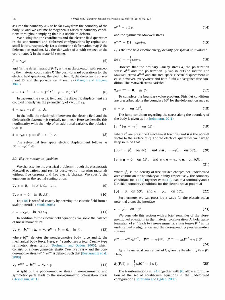
Fig. 1. Undeformed and deformed configuration of a nonlinearly deforming body immersed in free space.

F. Vogel et al. / European Journal of Mechanics A/Solids 48 (2014) 112e128 113

Mazza, 2005; Brochu and Pei, 2010; Hossain et al., 2012). Here, weintroduce a model, in which the electric field, governed by theelectrostatic Maxwell equations, affects both the mechanicalequilibrium equation and the viscous constitutive response. Typicalapplications are dielectric elastomers filled with particles to in-crease their electric permittivity (Mazzoldi et al., 2004), whichwere either fabricated in an electric field or are responsive to alignwith an electric field. A rotation of polar groups due to an externallyapplied electric field occurs in certain electrostrictive polymers(Brochu and Pei, 2010), which makes a consideration of thedielectric relaxation necessary (Khan et al., 2013).

We base our work on the well-established concepts withinelectro-elasticity (Dorfmann and Ogden, 2005, 2006; Bustamanteet al., 2009) built on the original works (Toupin, 1956; Truesdelland Toupin, 1960; Eringen, 1963; Lax and Nelson, 1971; Tiersten,1971; Maugin, 1977) and their advances in the last decade(Ericksen, 2007; Fosdick and Tang, 2007; McMeeking et al., 2007;Steigmann, 2009; Maugin, 2009). For the formulation of theviscous material model, we adopt the concept of internal variablesto capture the dissipative effects (Simo and Hughes, 1998; Reeseand Govindjee, 1998; Holzapfel, 2001). We assume an additivedecomposition of the free energy density into equilibrium andviscous parts (Reese and Govindjee, 1998). For the definition ofconstitutive relations and a linear evolution equation to determinethe internal variables, we work entirely in the logarithmic strainspace. This concept was initially developed and applied in thecontext of plasticity (Miehe and Lamprecht, 2001; Miehe et al.,2002, 2009, 2011; Germain et al., 2010) and allows for an additivesplit in logarithmic elastic and viscous strains.

This special structure enables us to use a viscous rheologicalmodel, which originally stems from the geometric linear theoryalthough we consider large deformations (El Sayed et al., 2008;Khan et al., 2013). Alternatively, we could adopt the multiplica-tive decomposition of the deformation gradient into elastic andviscous parts (Ask et al., 2012a, 2012b; Büschel et al., 2013). Incontrast to the usage of internal variables, a functional thermody-namic framework of electro-visco-elasticity would also be possible(Chen, 2010).

The numerical implementation of the model is realized within ageometrically non-linear finite element framework (Vu et al.,2007). We simulate several actuator geometries, such as extend-ing, bending and a diaphragm actuators, to show the performanceof the method including typical relaxation and creep behavior. Weperform a detailed parametric study that demonstrates the sensi-tivity of the model with regard to the choice of electro-viscous

coupling parameters. We illustrate that the incorporation of theelectric field into the viscous contribution significantly alters therelaxation and hysteresis behavior of the model.

2. Basic equations

The mathematical modeling of the mechanical elasticity prob-lem coupled with electrostatics has been treated in detail from theearly pioneering work (Toupin, 1956; ; Eringen, 1963; Lax andNelson, 1971; Tiersten, 1971; Maugin, 1977) up to the presentyears (Ericksen, 2007; Fosdick and Tang, 2007; McMeeking et al.,2007; Steigmann, 2009; Maugin, 2009). Here we expand the for-mulations presented by Ogden and co-workers (Dorfmann andOgden, 2005, 2006; Bustamante et al., 2009). To trace the origins,we briefly summarize the basic equations of nonlinear continuummechanics and electrostatics.

2.1. Preliminaries

We investigate a nonlinearly deforming body B immersed invacuum S, which is subject to an electric field as depicted in Fig. 1.Since the body may undergo large deformations, we distinguishbetween an undeformed configuration kv1 and a deformed config-uration Bt . For the material and spatial setting, we divide the sur-face of the body in two different ways (Bustamante, 2009), toprescribe mechanical and electric boundary conditions:

vB0 ¼ vB9

0WvB4

0 ¼ vBd0WvBt

0; vBt ¼ vB9tWvB4

t ¼ vBdt WvBt

t

(1)

such that

vB4sB; vB9XvB4 ¼ B; vBdXvBt ¼ B (2)

and

vS0 ¼ vSNWvB0; vSt ¼ vSNWvBt (3)

with

vSN ¼ vS9NWvS4

N; vS9NXvS4

N ¼ B: (4)

The boundary parts marked with the superscripts 9 and 4 denotethe electric Neumann and Dirichlet boundaries, respectively, andthe superscripts d and t denote their mechanical counterparts. We

F. Vogel et al. / European Journal of Mechanics A/Solids 48 (2014) 112e128114

assume the boundary vSN to be far away from the boundary of thebody vB and we assume homogeneous Dirichlet boundary condi-tions throughout, implying that it is unable to deform.

We distinguish the coordinates and the electric field quantitiesin the undeformed and deformed configurations by capital andsmall letters, respectively. Let 4 denote the deformation map, F thedeformation gradient, i.e., the derivative of 4 with respect to thecoordinates X in the material setting,

F ¼ VX4 (5)

and J is the determinant of F$VX is the nabla operator with respectto the material coordinates X. The push-forward operations for theelectric field quantities, the electric field E, the dielectric displace-ment D, and the polarization P read as (Maugin and Eringen,1990)

e ¼ E$F�1; d ¼ D$J�1FT ; p ¼ P$J�1FT : (6)

In vacuum, the electric field and the dielectric displacement arecoupled linearly via the permittivity of vacuum ε0,

d ¼ ε0 e ¼ : dε in St : (7)

In the bulk, the relationship between the electric field and thedielectric displacement is typically nonlinear. Herewe describe thisnonlinearity with the help of an additional variable, the polariza-tion p

d ¼ ε0eþ p ¼ : dε þ p in Bt : (8)

The referential free space electric displacement follows asDε ¼ ε0JC

�1$E.

2.2. Electro-mechanical problem

We characterize the electrical problem through the electrostaticMaxwell equations and restrict ourselves to insulating materialswithout free currents and free electric charges. We specify theequations in the spatial configuration:

Vx$d ¼ 0; in BtWSt ; and (9)

Vx � e ¼ 0; in BtWSt : (10)

Eq. (10) is satisfied exactly by deriving the electric field from ascalar potential (Monk, 2003)

e ¼ �Vx4; in BtWSt : (11)

In addition to the electric field equations, we solve the balanceof linear momentum

Vx$sþ bpont þ bt ¼ Vx$stot þ bt ¼ 0; in Bt ; (12)

where bpont denotes the ponderomotive body force and bt themechanical body force. Here, stot symbolizes a total Cauchy typesymmetric stress tensor (Dorfmann and Ogden, 2005), whichconsists of a non-symmetric elastic Cauchy stress s and the pon-deromotive stress spon. spon is defined such that (Bustamante et al.,2009)

Vx$spon ¼ bpont ¼ Vx e$p: (13)

A split of the ponderomotive stress in non-symmetric andsymmetric parts leads to the non-symmetric polarization stress(Steinmann, 2011)

spol ¼ e5p; (14)

and the symmetric Maxwell stress

smax ¼ Etiþ ε0e5e: (15)

Et is the free field electric energy density per spatial unit volume

EtðeÞ ¼ �12ε0e$e: (16)

Observe that the ordinary Cauchy stress s, the polarizationstress spol and the polarization p vanish outside matter. TheMaxwell stress smax and the free space electric displacement dε

exist, however, everywhere and both fulfill a divergence free con-dition. The Maxwell stress satisfies

Vx$smax ¼ 0; in St : (17)

To complete the boundary value problem, Dirichlet conditionsare prescribed along the boundary vBd

t for the deformation map 4:

4 ¼ 4p; on vBdt : (18)

The jump condition regarding the stress along the boundary ofthe body is given as in (Steinmann, 2011)

EstotF$n ¼ �tpt ; on vBtt ; (19)

where tpt are prescribed mechanical tractions and n is the normalvector to the surface of Bt . For the electrical quantities we have tokeep in mind that

EdF$n ¼ b9ft ; on vB9t ; and d$nN ¼ �b9fN; on vS9

N; (20)

EeF� n ¼ 0; on vBt ; and e� n ¼ eN � n; on vS4N;

(21)

where b9fN is the density of free surface charges per undeformedarea volume on the boundary at infinity, respectively. The boundaryconditions for e (21) together with (11), lead to a continuity and aDirichlet boundary conditions for the electric scalar potential

E4F ¼ 0; on vB9t ; and 4 ¼ 4N; on vS4

N: (22)

Furthermore, we can prescribe a value for the electric scalarpotential along the interface

4 ¼ 4p; on vB4t : (23)

We conclude this section with a brief reminder of the afore-mentioned equations in the material configuration. A Piola trans-formation of stot leads to a non-symmetric stress tensor Ptot in theundeformed configuration and the corresponding ponderomotivestresses

Ptot ¼ stot$JF�T ; Ppol ¼ e5P; Pmax ¼ E0F�T þ e5Dε:

(24)

E0 is the material counterpart of Et given by the identity E0 ¼ JEt.Thus,

E0ðF; EÞ ¼ �12ε0JC

�1 : ½E5E�: (25)

The transformations in (24) together with (6) allow a formula-tion of the set of equilibrium equations in the undeformedconfiguration (Dorfmann and Ogden, 2005):


VX$Ptot þ b0 ¼ 0; in B0; (26)

VX$Pmax ¼ 0; in S0; (27)

VX$D ¼ 0; in B0WS0; (28)

VX � E ¼ 0; in B0WS0; (29)

(29) is equivalent to the existence of a scalar potential such that

E ¼ �VX4; in B0WS0 (30)

and the boundary conditions are translated to

EPtotF$N ¼ �tp0; on vBt0; (31)

EDF$N ¼ 9f0; on vB9

0: (32)

3. Material model for electro-visco-elasticity

We investigate a material model for electro-active materialexhibiting viscous behavior. In our model, the electric field in-fluences the equilibrium elastic response and the viscous behaviorof the material at the same time. Thus, we consider mechanical anddielectric relaxation equally and develop a quite general modeladjustable to all kinds of electro-active materials. We propose anelectro-viscoelastic material model in the spirit of a transverselyisotropic material. Thereby, we define the axis of anisotropy alongthe direction to the electric field E. An imprinted preferred direc-tion or re-orientation during electric stimulation of electric dipoleswithin an electro-active material motivates this approach. This canapply to dielectric elastomers filled with particles to increase theirelectric permittivity (Mazzoldi et al., 2004), whose curing processtook place either under an electric field or for those, which consistof such a soft elastomeric matrix that the particles can align withthe electric field. A rotation of polar groups due to an externallyapplied electric field occurs in certain electrostrictive polymers(Brochu and Pei, 2010), which makes a consideration of thedielectric relaxation necessary (Khan et al., 2013).

3.1. Constitutive relations derived from the dissipation inequality

To simplify the definition of the constitutive equations, we as-sume the existence of an amended, augmented, or total free energy(Dorfmann and Ogden, 2005, 2006)

W0ðF; E;Q1;.;Q nÞ ¼ j0ðF; E;Q 1;.;QnÞ þ E0ðF;EÞ; (33)

depending on the deformation gradient F, the electric field E, and aset of the internal variables Q1,.,Qn for the incorporation of aviscous material model. The dissipation inequality based on (Pao,1978; Maugin and Eringen, 1990; Dorfmann and Ogden, 2003)reads after a Legendre transformation (Bustamante et al., 2009;Khan et al., 2013) as

D0 ¼ Ptot : _F �D$ _E� _W0ðF; E;Q1;.;Q nÞ � 0: (34)

Due to the additive split ofW0 into the strain energy function j0and the electric free field energy E0, we can separate the derivativesof E0 from the dissipation inequality and proceed directly to theconstitutive relations for the Maxwell stress and the free spaceelectric displacement:

Pmax ¼ vE0ðF; EÞvF

; Dε ¼ �vE0ðF; EÞvE

: (35)

To ensure the requirement of objectivity, we define the totalenergy in terms of C. Furthermore, we assume our material to beisotropic and electro-mechanically coupled. Thus, we can expressthe strain energy density in terms of six invariants I1 through I6corresponding to C and E5E (Spencer, 1971; Liu, 2002; Dorfmannand Ogden, 2005). With this at hand, we rewrite the dissipationinequality D0

0 in terms of the PiolaeKirchhoff stress S and fj0

D00 ¼

hP þ Ppol

i: _F � P$ _E� _j0ðF;E;Q1;.;QnÞ (36)

¼ 12

hS þ Spol

i: _C � P$ _E� _fj0ðC; E;Q1;.;Q nÞ � 0: (37)

fj0 is the re-parameterization of j0 such that

fj0ðC;E;Q 1;.;QnÞ ¼ fj0

�FT$F;E;Q1;.;Qn

�¼ j0ðF; E;Q1;.;QnÞ: (38)

For our desired material model, we combine two well-established principles encountered in visco-elasticity and plas-ticity: At first, we transfer to the logarithmic strain space and sec-ondly, we use an extended generalizedMaxwell model to representthe viscous material behavior.

The general concept roots in the definition of the logarithmicstrain tensor

ε ¼ 12ln C: (39)

After a second re-parameterization of j0 such that

cj0ðε;E;q1;.;qnÞ ¼ cj0

�12ln C; E;q1;.;qn

�

¼ fj0ðC; E;Q1;.;Q nÞ;

we can define the strain energy function in terms of the logarithmicstrain ε, the electric field E and the corresponding internal variablesq1,.qn. Working in the logarithmic strain space mimics the smallstrain format (Miehe and Lamprecht, 2001; Miehe et al., 2002;Germain et al., 2010). This special structure enables us to use arheological model for viscosity, which originally stems from thegeometric linear theory although we consider large deformations.

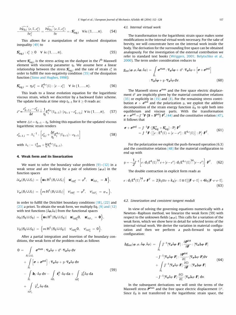
The generalized Maxwell model in 1d consists of a single Hoo-kean spring element with elastic modulus EN to represent theelastic equilibrium response in parallel to several Maxwell ele-ments with elastic moduli E1 through En to model the viscousresponse of the material (See Fig. 2). In order to extend thegeneralized Maxwell model to the coupled electro-mechanical 3dproblem, we propose that the energy stored within the springsdepends on the strain and the electric field. This approach isapplied to the equilibrium spring and to the springs in the viscousbranches. In 1d, this translates to Young’s moduliENðEÞ; E1ðEÞ;.; EnðEÞ that depend on the electric field.

We pursue a decoupled representation of the strain energydensity cj0 (Reese and Govindjee, 1998; Holzapfel, 2001) and splitcj0 additively into an equilibrium part cj0

Nand a viscous part cj0

v.

The equilibrium part cj0N

represents the strain energy density inthe electro-elastic Hooke element and cj0

vthe energy in the

electro-viscous Maxwell elements:

cj0ðε;E;q1;.;qnÞ ¼ cj0Nðε;EÞ þ cj0

vðε; E;q1;.;qnÞ: (40)

Fig. 2. Generalized Maxwell model for the one dimensional case with one Hookeanspring element and n Maxwell elements in parallel.


In the state of thermodynamical equilibrium, the springs of theMaxwell elements are relaxed and the total energy density consistsonly of the equilibrium part cj0

N.

The total logarithmic strain ε corresponds to the elongation ofthe equilibrium spring. As a special consequence of the lineartheory, the total strain can be split for each Maxwell element in theelastic logarithmic strain ε

e corresponding to the elongation of thespring and in the viscous logarithmic strain ε

v corresponding to theelongation of the dashpot. The resulting identity

ε ¼ εei þ ε

vi c i˛f1;.;ng (41)

motivates the identification of the internal variable qi with theviscous logarithmic strain ε

vi within the ith Maxwell element (Reese

and Govindjee, 1998; ). A formal change of the input variables leadsto a strain energy function of the form

cj0ðε;E; εv1;.; εvnÞ ¼ cj0Nðε; EÞ þ cj0

vðε; E; εv1;.; εvnÞ: (42)

In a final step, we transfer the pair of work conjugates(S þ Spol,C) from Eq. (37) to the logarithmic strain setting. For doingso, we introduce a fourth order transformation tensor

P ¼ 2vε

vC; (43)

and a logarithmic analog to the PiolaeKirchhoff stress

Slog þ Spollog :¼hS þ Spol

i: P�1: (44)

Rewriting _C in terms of P and ε, modifies the dissipationinequality (37) to

D000 ¼

hSlog þ Spollog

i: _ε� P$ _E� _cj0ðε; E; εv1;.; εvnÞ � 0: (45)

From here, we derive constitutive relations with the help of theColemaneNoll procedure

Slog þ Spollog ¼ vcj0ðε; E; εv1;.; εvnÞvε

; P ¼ �vcj0ðε; E; εv1;.; εvnÞvE

:

(46)

Using the additive split of the strain energy density in (40), wecan define a separation of the stress tensor Slog þ Spollog and P inequilibrium and viscous parts:

SNlog ¼hSlogþ Spollog

iN ¼ vcj0Nðε;EÞvε

; Svlog ¼hSlogþ Spollog

iv

¼ vcj0vðε;E;εv1;.;εvnÞ

vε; (47)

PN ¼ �vcj0Nðε;EÞvE

; Pv ¼ �vcj0vðε; E; εv1;.; εvnÞ

vE: (48)

The remaining reduced dissipation inequality for the logarith-mic viscous strain reads as

Dred0 ¼ �

Xni¼1

vcj0vðε;E; εv1;.; εvnÞ

vεvi: _εvi � 0: (49)

3.2. Explicit choice for the energy density functions

We consider a generalized Maxwell model with n independentMaxwell elements arranged in parallel. Thus, we can define a strainenergy function dj0;i

vfor each Maxwell element separately, which

sum up to the viscous strain energy cj0v:

cj0vðε; E; εv1;.ε

vnÞ ¼

Xni

dj0;ivðε;E; εvi Þ: (50)

As in the small deformation regime, cj0N

and dj0;ivare quadratic

functions in the total logarithmic strain ε and the elastic logarith-mic strain ε

ei (Reese and Govindjee, 1998; Holzapfel, 2001),

respectively. With Eq. (41), we can express this directly as

cj0Nðε;EÞ ¼ 1

2ε : E4ðEÞ : εþ c1I : E5Eþ c2ε : E5E; (51)

dj0;ivðε;E; εvi Þ ¼

12½ε� ε

vi � : E4;vðEÞ : ½ε� ε

vi � ci˛f1;.;ng: (52)

Besides the quadratic term in the logarithmic strains, weamended the equilibrium energy cj0

Nby two terms corresponding

to the invariants I4 ¼ I : E5E and I5 ¼ C : E5E, which are respon-sible for the polarization and the electrostrictive effect (Maugin andEringen, 1990), respectively. The coupling parameters have to fulfillthe conditions c1 < 0 and c2 > 0 to guarantee a reasonable orien-tation of D in comparison to E and a contraction of the materialwithin the direction of E.

We use here the definition of the transversely isotropic fourth-order tensor E4ðEÞ

E4ðEÞ : ¼ ke1I5I þ ke2 14sym þ ke3½I5kþ k5I�þ ke4k5kþ ke5

�I5kþ I5kþ k5I þ k5I

� (53)

with the anisotropic (structural) tensor k ¼ E5E. E4,v followsthe same definition with its constants kv1 through kv5. To clarifynotation, we used the non-standard dyadic products of any twosecond order tensor: A5B ¼ AikBjlei5ej5ek5el and A5B ¼AilBjkei5ej5ek5el . With this, the symmetric fourth order unittensor reads as 14sym ¼ 1

2 ½I5I þ I5I�.

3.3. Evolution equation for the internal variables

Comparing the derivatives of the viscous strain energy functionEq. (52) with respect to the logarithmic strain tensors, leads to theidentity


�vdj0;ivðε;E;εvi Þ ¼ vdj0;i

vðε;E;εvi Þ ¼ : Sv ci˛f1;.;ng: (54)
vεvi vε log;i
This allows for a manipulation of the reduced dissipationinequality (49) to

Svlog;i : _εvi � 0 c i˛f1;.;ng; (55)

where Svlog;i is the stress acting on the dashpot in the ith Maxwellelement with viscosity parameter hi. We assume here a linearrelationship between the stress Svlog;i and the rate of strain _εvi inorder to fulfill the non-negativity condition (55) of the dissipationfunction (Simo and Hughes, 1998):

Svlog;i ¼ hi _εvi ¼ E4;vi ðEÞ : ½ε� ε

vi � c i˛f1;.;ng: (56)

This leads to a linear evolution equation for the logarithmicviscous strain, which we discretize by a backward Euler scheme.The update formula at time step tkþ1 for k � 0 reads as:

_εvzεvkþ1;i�ε

vk;i

Dt¼! 1

hiE4;vi ðEkþ1Þ : ½εkþ1�ε

vkþ1;i� c i˛f1;.;ng; (57)

where6t ¼ tkþ1 � tk. Solving this equation for the updated viscouslogarithmic strain renders

εvkþ1;i ¼ A�1

i :

�εvk;i þ

DthiE4;vi ðEkþ1Þ : εkþ1

(58)

with Ai :¼ 14sym þ DthiE4;vi ðEkþ1Þ:

4. Weak form and its linearization

We want to solve the boundary value problem (9)e(12) in aweak sense and are looking for a pair of solutions (4,4) in thefunction spaces

U4ðBtWStÞ ¼nu˛H1ðBtWStÞ

ujvBdt¼ 4P; ujvSN

¼ Xo;

V4ðBtWStÞ ¼nv˛H1ðBtWStÞ

vjvB4

t¼ 4P; vjvS4

N¼ 4N

o;

in order to fulfill the Dirichlet boundary conditions (18), (22) and(23) a priori. To obtain the weak form, we multiply Eq. (9) and (12)with test functions (d4,d4) from the functional spaces

U0ðB0WS0Þ ¼nu˛H1ðB0WS0Þj uj

vBd00; ujvSN

¼ 0o;

V0ðB0WS0Þ ¼nv˛H1ðB0WS0Þj vjvB4

00; vjvS4

0¼ 0

o:

After a partial integration and insertion of the boundary con-ditions, the weak form of the problem reads as follows

0 ¼Z

BtWSt

smax : Vxd4þ dε$Vxd4 dv

þZBt

hsþ spol

i: Vxd4þ p$Vxd4 dv

�ZBt

bt$d4 dv�ZvBt

tpt $d4 daþZvB9

t

b9ftd4 da

þZ

vS9N

b9fNd4 da:

(59)

4.1. Internal virtual work

The transformation to the logarithmic strain space makes somemodifications in the internal virtual work necessary. For the sake ofbrevity, we will concentrate here on the internal work inside thebody. The derivation for the surrounding free space can be obtainedanalogously. For the investigation of the external contribution werefer to standard text books (Wriggers, 2001; Belytschko et al.,2000). The term under consideration reduces to

gintð4;4;d4;d4Þ ¼ZBt

smax :Vxd4þ dε$Vxd4þhsþspol

i

:Vxd4þp$Vxd4dv: (60)

The Maxwell stress smax and the free space electric displace-ment dε are implicitly given by the material constitutive relations(35) or explicitly in (15) and (8). For the remaining stress contri-bution s þ spol and the polarization p, we exploit the additivedecomposition of the strain energy function cj0 to split both intoequilibrium and viscous parts. With the transformations þ spol ¼ J�1F$[S þ Spol]$FT, (44) and the constitutive relation (47),it follows that

sþ spol ¼ J�1F$½½SNlog þ Svlog� : P�$FT

¼ J�1F$��ε : E4ðEÞ þ ½ε� ε

v� : E4;vðEÞ� : P�$FT :(61)

For the polarizationwe exploit the push-forward operation (6.3)and the constitutive relation (48) for the material configuration toend up with

p¼�12J�1

�ε :dEE4ðEÞ :34 εþ½ε�ε

v� :dEE4;vðEÞ :34 ½ε�εv�$FT : (62)

The double contraction in explicit form reads as

ε : dEE4ðEÞ :34 ε$FT ¼ 2½k3trεþ k4½ε : E5E��½F$ε$E� þ 4k5½F$ε$ε$E�:(63)

4.2. Linearization and consistent tangent moduli

In view of solving the governing equations numerically with aNewtoneRaphson method, we linearize the weak form (59) withrespect to the unknown fields (4,4). This calls for a variation of theweak form, which we show here in detail for selected terms of theinternal virtual work. We derive the variation in material configu-ration and then we perform a push-forward to spatialconfiguration:

Dgintð4;4; d4; d4Þ ¼ZBt

J�1½Vxd4$F� : vPtot

vF: ½VxD4$F�

� J�1½Vxd4$F� : vPtot

vE$½VxD4$F�dv

þZBt

J�1½Vxd4$F�$vDvF

: ½VxD4$F�

� J�1½Vxd4$F�$vDvE

$½VxD4$F� dv:

(64)

In the subsequent derivations we will omit the terms of theMaxwell stress Pmax and the free space electric displacement Dε.Since E0 is not transferred to the logarithmic strain space, the


contributions of Pmax andDε to the variation consist of the standardsecond order derivatives of E0. For the remaining terms, a mappinginto the logarithmic strain space yields the following expression

Dgredint ð4;4; d4; d4Þ ¼ZBt

Vxd4 : I5hsþ spol

i: VxD4 dv

þZBt

Vxd4 : J�1½F5F� :hPT : Ta : P

þ ½SNlog þ Svlog� : Li:hFT5FT

i: VxD4 dv

�ZBt

Vxd4 : J�1½F5F� :hPT : Tk

i$FT$VxD4 dv

þZBt

Vxd4$J�1F$½TTk : P� :

hFT5FT

i: VxD4 dv

�ZBt

Vxd4$J�1F$Tb$FT$VxD4 dv

(65)

with

L ¼ 4v2ε

vC2 : (66)

A detailed definition including algorithms for implementingfourth-order tensor P and the double contraction of the sixth-ordertensor L with ½SNlog þ Svlog� can be found in Miehe and Lamprecht(2001), Miehe et al. (2002). The geometric tangent in the firstrow of (65), can be evaluated once we know the correspondingstresses (Reese and Govindjee, 1998). The remaining four integralsform the constitutive tangent, for which an algorithmicallyconsistent derivation is necessary to preserve the quadraticconvergence of NewtoneRaphson scheme (Simo and Taylor, 1985; ;Wriggers, 2001; Belytschko et al., 2000). Besides the stress tangentTa (Miehe and Lamprecht, 2001; Miehe et al., 2002),

Ta ¼ v½SNlog þ Svlog�vε

¼ v2cj0Nðε; EÞvε2

þ dεSvlog; (67)

dεSvlog :¼ vSvlog;kþ1

vεkþ1¼ E4;vðEkþ1Þ :

h14sym � dεεvkþ1

i; (68)

we introduce the electro-mechanical coupling tangent Tk

Tk ¼ v½SNlog þ Svlog�vE

¼ v2cj0Nðε; EÞ

vEvεþ dESvlog; (69)

dESvlog :¼vSvlog;kþ1

vEkþ1¼ ½εkþ1�ε

vkþ1� :dEE4;vðEkþ1Þ�E4;vðEkþ1Þ

:dEεvkþ1; (70)

and the purely electrical tangent Tb such that:

Tb ¼ v½PN þ Pv�vE

¼ �v2cj0Nðε; EÞvE2

þ dEPv; (71)

dEPv :¼ vPvkþ1

vEkþ1¼ ½εkþ1 � ε

vkþ1�

: dEE4;vðEkþ1Þ :34

dEεvkþ1 �12½εkþ1 � ε

vkþ1�

: d2E EE4;vðEkþ1Þ :

34 ½εkþ1 � εvkþ1�: (72)

For our specific choice of the update for the internal variable(58), the algorithmically consistent derivation of the logarithmicstrain tensor εvkþ1 with respect to εkþ1 results in

dεεvkþ1 :¼ vεvkþ1vεkþ1

¼ DthA�1 : E4;vðEkþ1Þ; : (73)

With dEεkþ1 ¼ 0, it follows for the derivative with respect to Ekþ1that

dEεvkþ1 :¼ vεvkþ1vEkþ1

¼ DthA�1 : dEE4;vðEkþ1Þ :

34 ½εkþ1 � εvkþ1�; (74)

where the second double contraction is defined for any fifth ordertensor A and fourth order tensor B as A :

34B ¼

AijklmBklpqei5ej5em5ep5eq. The algorithmic derivativesdEE4;vðEkþ1Þ and d2

E EE4;vðEkþ1Þ coincide with the ordinary contin-

uum derivatives vE4;vðEÞ=vE and v2E4;vðEÞ=vE2.

5. Numerical results

As prototype for our numerical examples serves a bulk ofdielectric elastomer under the stimulation of an electric field. In areal world experiment, two compliant electrodes are adhered tothe dielectric material and the applied electric voltage betweenthe electrodes causes a field activated bulk deformation. Thismovement is useful to set up electro-active materials as actuatorsof different kind. Although this might not be feasible for all sets ofexperiments (Begley et al., 2005), we ignore the compliant elec-trodes within the finite element model due to their negligiblethickness in comparison to the polymer film (Pelrine et al., 1998;Begley et al., 2005) and the assumption of perfect adhesion(O’Halloran et al., 2008). All numerical experiments were per-formed with an in-house finite element code implemented inFORTRAN90 where the electro-visco-elastic material model hasbeen incorporated. Standard displacement based hexahedralfinite elements have been used throughout the simulations.

As a first numerical example, we consider a thin film of dielec-tric elastomer immersed into an electric field to calibrate thecoupling parameters c1 and c2. Next, we perform a detailed para-metric study of the constants kv3, k

v4, and kv5 in the material tensor

E4,v by analyzing the relaxation and hysteresis tests of a thin plate.Both setups resemble an extending actuator. Finally, we study abimorph bending actuator where we put special emphasis to thelarge deformations of the structure and the creep behavior due toviscosity. We restrict ourselves to an investigation containing asingle Maxwell element. Table 1 summarizes the set of materialparameters, from which the mechanical parameters in E4 and E4,v

can be calculated as ke1 ¼ kv1 ¼ k� 23m and ke2 ¼ kv2 ¼ m. For the

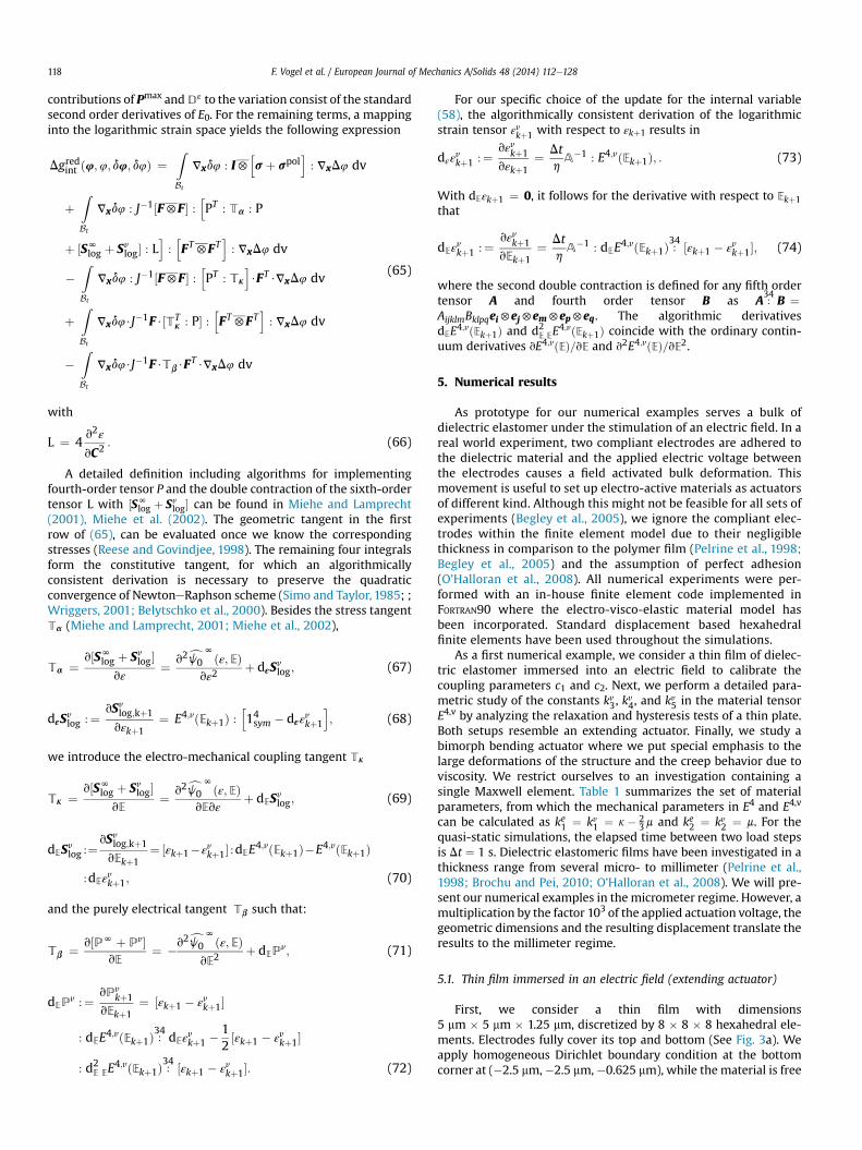
quasi-static simulations, the elapsed time between two load stepsis Dt ¼ 1 s. Dielectric elastomeric films have been investigated in athickness range from several micro- to millimeter (Pelrine et al.,1998; Brochu and Pei, 2010; O’Halloran et al., 2008). We will pre-sent our numerical examples in the micrometer regime. However, amultiplication by the factor 103 of the applied actuation voltage, thegeometric dimensions and the resulting displacement translate theresults to the millimeter regime.

5.1. Thin film immersed in an electric field (extending actuator)

First, we consider a thin film with dimensions5 mm � 5 mm � 1.25 mm, discretized by 8 � 8 � 8 hexahedral ele-ments. Electrodes fully cover its top and bottom (See Fig. 3a). Weapply homogeneous Dirichlet boundary condition at the bottomcorner at (�2.5 mm,�2.5 mm,�0.625 mm), while the material is free

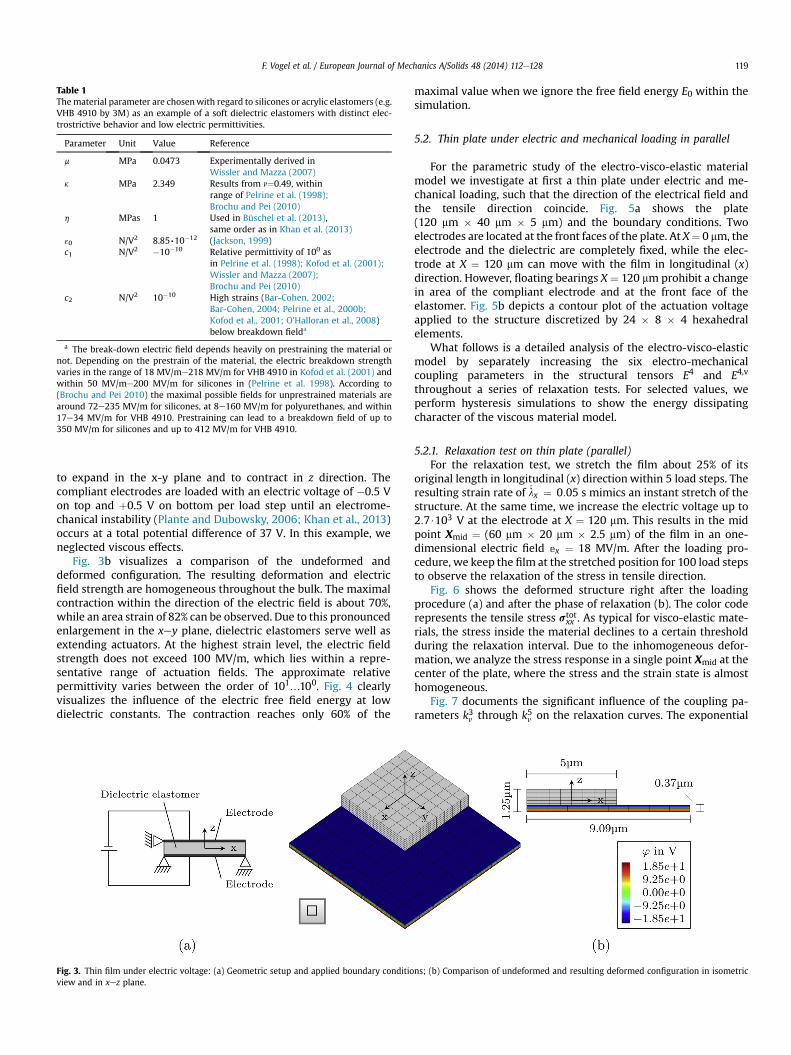
Table 1Thematerial parameter are chosenwith regard to silicones or acrylic elastomers (e.g.VHB 4910 by 3M) as an example of a soft dielectric elastomers with distinct elec-trostrictive behavior and low electric permittivities.

Parameter Unit Value Reference

m MPa 0.0473 Experimentally derived inWissler and Mazza (2007)

k MPa 2.349 Results from n¼0.49, withinrange of Pelrine et al. (1998);Brochu and Pei (2010)

h MPas 1 Used in Büschel et al. (2013),same order as in Khan et al. (2013)

ε0 N/V2 8.85,10�12 (Jackson, 1999)c1 N/V2 �10�10 Relative permittivity of 100 as

in Pelrine et al. (1998); Kofod et al. (2001);Wissler and Mazza (2007);Brochu and Pei (2010)

c2 N/V2 10�10 High strains (Bar-Cohen, 2002;Bar-Cohen, 2004; Pelrine et al., 2000b;Kofod et al., 2001; O’Halloran et al., 2008)below breakdown fielda

a The break-down electric field depends heavily on prestraining the material ornot. Depending on the prestrain of the material, the electric breakdown strengthvaries in the range of 18 MV/me218 MV/m for VHB 4910 in Kofod et al. (2001) andwithin 50 MV/me200 MV/m for silicones in (Pelrine et al. 1998). According to(Brochu and Pei 2010) the maximal possible fields for unprestrained materials arearound 72e235 MV/m for silicones, at 8e160 MV/m for polyurethanes, and within17e34 MV/m for VHB 4910. Prestraining can lead to a breakdown field of up to350 MV/m for silicones and up to 412 MV/m for VHB 4910.


to expand in the x-y plane and to contract in z direction. Thecompliant electrodes are loaded with an electric voltage of �0.5 Von top and þ0.5 V on bottom per load step until an electrome-chanical instability (Plante and Dubowsky, 2006; Khan et al., 2013)occurs at a total potential difference of 37 V. In this example, weneglected viscous effects.

Fig. 3b visualizes a comparison of the undeformed anddeformed configuration. The resulting deformation and electricfield strength are homogeneous throughout the bulk. The maximalcontraction within the direction of the electric field is about 70%,while an area strain of 82% can be observed. Due to this pronouncedenlargement in the xey plane, dielectric elastomers serve well asextending actuators. At the highest strain level, the electric fieldstrength does not exceed 100 MV/m, which lies within a repre-sentative range of actuation fields. The approximate relativepermittivity varies between the order of 101.100. Fig. 4 clearlyvisualizes the influence of the electric free field energy at lowdielectric constants. The contraction reaches only 60% of the

Fig. 3. Thin film under electric voltage: (a) Geometric setup and applied boundary conditioview and in xez plane.

maximal value when we ignore the free field energy E0 within thesimulation.

5.2. Thin plate under electric and mechanical loading in parallel

For the parametric study of the electro-visco-elastic materialmodel we investigate at first a thin plate under electric and me-chanical loading, such that the direction of the electrical field andthe tensile direction coincide. Fig. 5a shows the plate(120 mm � 40 mm � 5 mm) and the boundary conditions. Twoelectrodes are located at the front faces of the plate. At X¼ 0 mm, theelectrode and the dielectric are completely fixed, while the elec-trode at X ¼ 120 mm can move with the film in longitudinal (x)direction. However, floating bearings X ¼ 120 mm prohibit a changein area of the compliant electrode and at the front face of theelastomer. Fig. 5b depicts a contour plot of the actuation voltageapplied to the structure discretized by 24 � 8 � 4 hexahedralelements.

What follows is a detailed analysis of the electro-visco-elasticmodel by separately increasing the six electro-mechanicalcoupling parameters in the structural tensors E4 and E4,v

throughout a series of relaxation tests. For selected values, weperform hysteresis simulations to show the energy dissipatingcharacter of the viscous material model.

5.2.1. Relaxation test on thin plate (parallel)For the relaxation test, we stretch the film about 25% of its

original length in longitudinal (x) direction within 5 load steps. Theresulting strain rate of _lx ¼ 0:05 s mimics an instant stretch of thestructure. At the same time, we increase the electric voltage up to2:7$103 V at the electrode at X ¼ 120 mm. This results in the midpoint Xmid ¼ (60 mm � 20 mm � 2.5 mm) of the film in an one-dimensional electric field ex ¼ 18 MV/m. After the loading pro-cedure, we keep the film at the stretched position for 100 load stepsto observe the relaxation of the stress in tensile direction.

Fig. 6 shows the deformed structure right after the loadingprocedure (a) and after the phase of relaxation (b). The color coderepresents the tensile stress stot

xx . As typical for visco-elastic mate-rials, the stress inside the material declines to a certain thresholdduring the relaxation interval. Due to the inhomogeneous defor-mation, we analyze the stress response in a single point Xmid at thecenter of the plate, where the stress and the strain state is almosthomogeneous.

Fig. 7 documents the significant influence of the coupling pa-rameters k3v through k5v on the relaxation curves. The exponential

ns; (b) Comparison of undeformed and resulting deformed configuration in isometric

Fig. 4. Thin film under electric voltage from D4 ¼ 0 V to D4 ¼ 37 V: Plot of evolution of stretch lz and electric displacement dz over electric field ez with and without considerationof the free field electric energy E0.


decrease in tensile stress illustrates the viscous material response.The curves show that the material reaches a completely relaxedstate already after 50 steps of relaxation. Furthermore, the totalstress response is higher as soon as an electric field is applied. Thisis due to the compliant electrodes, which tend to attract each otherand thus exert a ponderomotive stress on the bulk. This compres-sive stress hinders the stretching of the material. Fig. 7a shows thatan increase in k3v leads to a relaxation process already during theloading phase. For high values of k3v , the material is at a relaxedstate by the time the loading path is completed. Thus, the materialbehaves more and more elastic or in other words, an increase of k3vleads to a decrease in the corresponding viscosity parameter. Fig. 7band c illustrate that, in contrast to Fig. 7a, increasing the values of k4vand k5v yields an overall stiffer material response and a decrease inrelaxation time. Relaxation takes place at a much faster rate as inthe experiments when k4v and k5v were set to zero.

5.2.2. Hysteresis test on thin plate (parallel)For the hysteresis tests, we first stretch thematerial about 25% of

its original length followed by a compression via the neutral posi-tion until the structure has shortened in longitudinal directionabout 25% of its original length. Fig. 8 illustrates the fully elongated(a), compressed (b) and neutral position (c). We repeat this loopthree times to reach the steady state and perform it at two differentstrain rates of _lx ¼ 0:01 s�1 and _lx ¼ 0:02 s�1. Thus, one hysteresisloop consists of 100 or 50 increments corresponding to 100 or 50 s.The simulation closes with 100 relaxation steps, during which thestructure recovers its initial configuration.

Fig. 5. Thin plate (120 mm � 40 mm � 5 mm) under electric voltage such that electric field isconditions; (b) Electric potential on discretized plate.

Within the very first 5 load steps, we apply two different actu-ation voltages of 5:4$102 V and 1:08$103 V, which equals a totalpotential difference of D4 ¼ 2:7$103Df¼2.7$103 V and 5:4$103 V.At full elongation, this results in the mid point Xmid of the film in anone-dimensional electric field of ex ¼ 18 MV/m and ex ¼ 36 MV/m.

Fig. 9 summarizes the evolution of the longitudinal stress stotxx

over stretch lx for diverse loadings and material parameters. Weconclude that the stronger the applied electric field, the higher thehysteresis curve is shifted translationally upwards along the y-axis.When no electric field is applied, the curve circles symmetricallyaround the origin with equally distributed periods of pull andcompression. However, under the influence of an electric field,which leads to a contraction of the material in x-direction, thephase of pull prevails. For even higher fields, the hysteresis curvelies completely in the positive stress range. Independent of thestrength of the electric field, the inclination of the hysteresis curveincreases for higher strain rates because at faster loading pro-cedures less relaxation takes places during the elongation of theplate. As a consequence, the maximum value of the longitudinalstress can be significantly higher.

Fig. 9bed document the effects of alternating the viscouscoupling parameters kv3 through kv5 during the hysteresis experi-ments. The results are well in line with the relaxation tests. Sinceincreasing of k3v leads to a relaxation process already during theloading phase, the material behaves more and more elastic. Fig. 9bshows a decrease in area enclosed by the hystereses as k3v increases.This is contrary to the observed changes in Fig. 9c and d, when

directed parallel to the mechanical loading: (a) Geometric setup and applied boundary

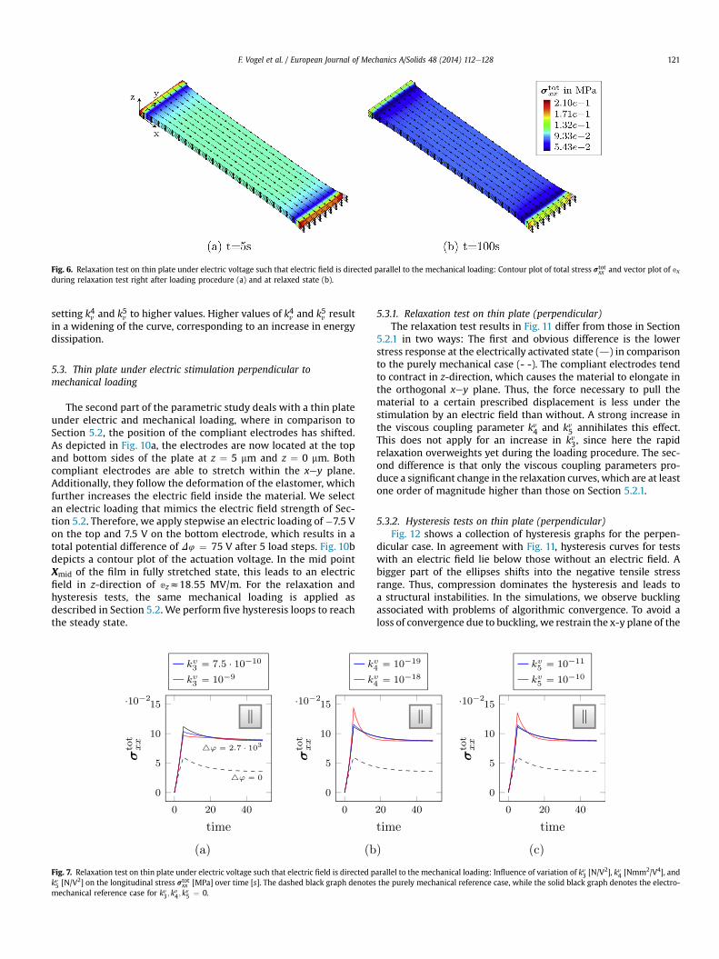
Fig. 6. Relaxation test on thin plate under electric voltage such that electric field is directed parallel to the mechanical loading: Contour plot of total stress stotxx and vector plot of ex

during relaxation test right after loading procedure (a) and at relaxed state (b).


setting k4v and k5v to higher values. Higher values of k4v and k5v resultin a widening of the curve, corresponding to an increase in energydissipation.

5.3. Thin plate under electric stimulation perpendicular tomechanical loading

The second part of the parametric study deals with a thin plateunder electric and mechanical loading, where in comparison toSection 5.2, the position of the compliant electrodes has shifted.As depicted in Fig. 10a, the electrodes are now located at the topand bottom sides of the plate at z ¼ 5 mm and z ¼ 0 mm. Bothcompliant electrodes are able to stretch within the xey plane.Additionally, they follow the deformation of the elastomer, whichfurther increases the electric field inside the material. We selectan electric loading that mimics the electric field strength of Sec-tion 5.2. Therefore, we apply stepwise an electric loading of �7.5 Von the top and 7.5 V on the bottom electrode, which results in atotal potential difference of D4 ¼ 75 V after 5 load steps. Fig. 10bdepicts a contour plot of the actuation voltage. In the mid pointXmid of the film in fully stretched state, this leads to an electricfield in z-direction of ezz18:55 MV/m. For the relaxation andhysteresis tests, the same mechanical loading is applied asdescribed in Section 5.2. We perform five hysteresis loops to reachthe steady state.

Fig. 7. Relaxation test on thin plate under electric voltage such that electric field is directed pkv5 [N/V2] on the longitudinal stress stot

xx [MPa] over time [s]. The dashed black graph denotesmechanical reference case for kv3; k

v4; k

v5 ¼ 0.

5.3.1. Relaxation test on thin plate (perpendicular)The relaxation test results in Fig. 11 differ from those in Section

5.2.1 in two ways: The first and obvious difference is the lowerstress response at the electrically activated state (d) in comparisonto the purely mechanical case (- -). The compliant electrodes tendto contract in z-direction, which causes the material to elongate inthe orthogonal xey plane. Thus, the force necessary to pull thematerial to a certain prescribed displacement is less under thestimulation by an electric field than without. A strong increase inthe viscous coupling parameter kv4 and kv5 annihilates this effect.This does not apply for an increase in kv3, since here the rapidrelaxation overweights yet during the loading procedure. The sec-ond difference is that only the viscous coupling parameters pro-duce a significant change in the relaxation curves, which are at leastone order of magnitude higher than those on Section 5.2.1.

5.3.2. Hysteresis tests on thin plate (perpendicular)Fig. 12 shows a collection of hysteresis graphs for the perpen-

dicular case. In agreement with Fig. 11, hysteresis curves for testswith an electric field lie below those without an electric field. Abigger part of the ellipses shifts into the negative tensile stressrange. Thus, compression dominates the hysteresis and leads toa structural instabilities. In the simulations, we observe bucklingassociated with problems of algorithmic convergence. To avoid aloss of convergence due to buckling, we restrain the x-y plane of the

arallel to the mechanical loading: Influence of variation of kv3 [N/V2], kv4 [Nmm2/V4], andthe purely mechanical reference case, while the solid black graph denotes the electro-

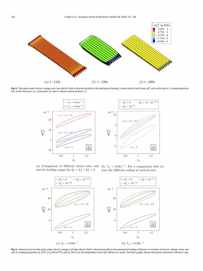
Fig. 8. Thin plate under electric voltage such that electric field is directed parallel to the mechanical loading: Contour plot of total stress stotxx and vector plot of ex during hysteresis

test at full extension (a), contraction (b) and in relaxed neutral position (c).

Fig. 9. Hysteresis test on thin plate under electric voltage such that electric field is directed parallel to the mechanical loading: Influence of variation of electric voltage, strain rateand of coupling parameter kv3 [N/V2], kv4 [Nmm2/V4], and kv5 [N/V2] on the longitudinal stress stot

xx [MPa] over strain. The black graphs denote the purely mechanical reference case.


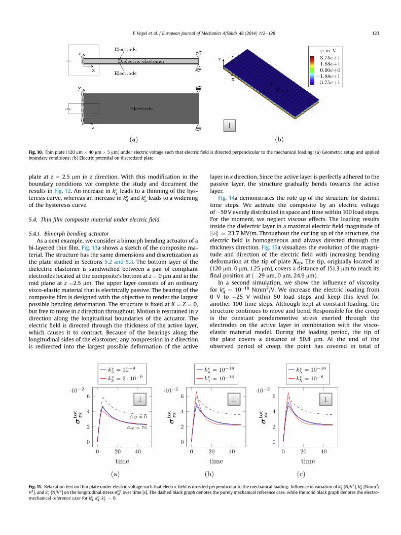
Fig. 10. Thin plate (120 mm � 40 mm � 5 mm) under electric voltage such that electric field is directed perpendicular to the mechanical loading: (a) Geometric setup and appliedboundary conditions; (b) Electric potential on discretized plate.


plate at z ¼ 2.5 mm in z direction. With this modification in theboundary conditions we complete the study and document theresults in Fig. 12. An increase in kv3 leads to a thinning of the hys-teresis curve, whereas an increase in kv4 and kv5 leads to a wideningof the hysteresis curve.

5.4. Thin film composite material under electric field

5.4.1. Bimorph bending actuatorAs a next example, we consider a bimorph bending actuator of a

bi-layered thin film. Fig. 13a shows a sketch of the composite ma-terial. The structure has the same dimensions and discretization asthe plate studied in Sections 5.2 and 5.3. The bottom layer of thedielectric elastomer is sandwiched between a pair of compliantelectrodes located at the composite’s bottom at z¼ 0 mm and in themid plane at z ¼2.5 mm. The upper layer consists of an ordinaryvisco-elastic material that is electrically passive. The bearing of thecomposite film is designed with the objective to render the largestpossible bending deformation. The structure is fixed at X ¼ Z ¼ 0,but free to move in z direction throughout. Motion is restrained in ydirection along the longitudinal boundaries of the actuator. Theelectric field is directed through the thickness of the active layer,which causes it to contract. Because of the bearings along thelongitudinal sides of the elastomer, any compression in z directionis redirected into the largest possible deformation of the active

Fig. 11. Relaxation test on thin plate under electric voltage such that electric field is directedV4], and kv5 [N/V2] on the longitudinal stress stot

xx over time [s]. The dashed black graph denotemechanical reference case for kv3; k

v4; k

v5 ¼ 0.

layer in x direction. Since the active layer is perfectly adhered to thepassive layer, the structure gradually bends towards the activelayer.

Fig. 14a demonstrates the role up of the structure for distincttime steps. We activate the composite by an electric voltageof�50 V evenly distributed in space and timewithin 100 load steps.For the moment, we neglect viscous effects. The loading resultsinside the dielectric layer in a maximal electric field magnitude ofkek ¼ 23:7 MV/m. Throughout the curling up of the structure, theelectric field is homogeneous and always directed through thethickness direction. Fig. 15a visualizes the evolution of the magni-tude and direction of the electric field with increasing bendingdeformation at the tip of plate Xtip. The tip, originally located at(120 mm, 0 mm, 1.25 mm), covers a distance of 151.3 mm to reach itsfinal position at (�29 mm, 0 mm, 24.9 mm).

In a second simulation, we show the influence of viscosityfor kv4 ¼ 10�18 Nmm2/V. We increase the electric loading from0 V to �25 V within 50 load steps and keep this level foranother 100 time steps. Although kept at constant loading, thestructure continues to move and bend. Responsible for the creepis the constant ponderomotive stress exerted through theelectrodes on the active layer in combination with the visco-elastic material model. During the loading period, the tip ofthe plate covers a distance of 50.8 mm. At the end of theobserved period of creep, the point has covered in total of

perpendicular to the mechanical loading: Influence of variation of kv3 [N/V2], kv4 [Nmm2/s the purely mechanical reference case, while the solid black graph denotes the electro-

Fig. 12. Hysteresis test on thin plate under electric voltage of D4 ¼ 75 V such that electric field is directed perpendicular to the mechanical loading: Influence of variation of strainrate and of coupling parameter kv3 [N/V2], kv4 [Nmm2/V4], and kv5 [N/V2] on the longitudinal stress stot

xx [MPa] over strain. The black graphs denote the purely mechanical referencecase.

Fig. 13. Bending actuator under electric voltage such that electric field is directed in thickness direction: (a) Geometric setup and applied boundary conditions; (b) discretizedcomposite plate.


Fig. 14. Bending actuator under electric voltage such that electric field is directed in thickness direction: Deformation due to applied voltage.


62.6 mm. Overall, the mechanism of creep causes additionaldeformation of about 23%, which might be crucial in the designof real world actuators.

In a third simulation, we rotate the actuator about 90 degreesaround the positive z-axis such that the x- and y-dimensions of theplate flip around to (40 mm, 120 mm, 5 mm). Xtip is now located at(40 mm, 0 mm, 1.25 mm). We repeat the electrical loading as beforeand observe a bending towards the longitudinal side of the

Fig. 15. Bending actuator under electric voltage such that electric field is directed in thickndeformation observed at Xtip.

actuator. Fig.14b illustrates the gradual deformation of the flat platetowards a tube. An additional bending of about 17% takes placeduring the relaxation period, which has to be considered for thelayout of a technical device.

5.4.2. Diaphragm actuatorFor our final example, we modify the mechanical boundary

condition of the bending actuator in Section 5.4.1 such that a

ess direction: (a) Evolution of electric field with time and (b) influence of viscosity on

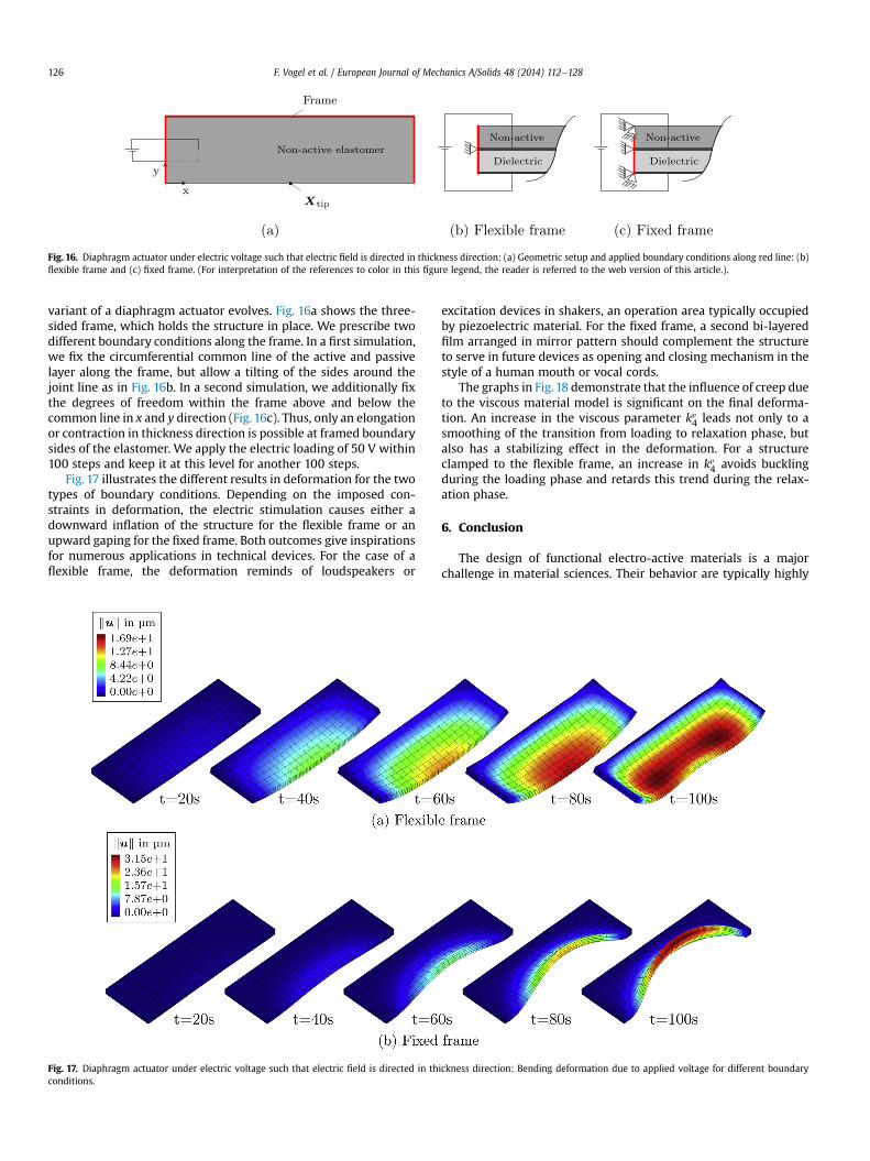
Fig. 16. Diaphragm actuator under electric voltage such that electric field is directed in thickness direction: (a) Geometric setup and applied boundary conditions along red line: (b)flexible frame and (c) fixed frame. (For interpretation of the references to color in this figure legend, the reader is referred to the web version of this article.).


variant of a diaphragm actuator evolves. Fig. 16a shows the three-sided frame, which holds the structure in place. We prescribe twodifferent boundary conditions along the frame. In a first simulation,we fix the circumferential common line of the active and passivelayer along the frame, but allow a tilting of the sides around thejoint line as in Fig. 16b. In a second simulation, we additionally fixthe degrees of freedom within the frame above and below thecommon line in x and y direction (Fig.16c). Thus, only an elongationor contraction in thickness direction is possible at framed boundarysides of the elastomer. We apply the electric loading of 50 V within100 steps and keep it at this level for another 100 steps.

Fig. 17 illustrates the different results in deformation for the twotypes of boundary conditions. Depending on the imposed con-straints in deformation, the electric stimulation causes either adownward inflation of the structure for the flexible frame or anupward gaping for the fixed frame. Both outcomes give inspirationsfor numerous applications in technical devices. For the case of aflexible frame, the deformation reminds of loudspeakers or

Fig. 17. Diaphragm actuator under electric voltage such that electric field is directed in thconditions.

excitation devices in shakers, an operation area typically occupiedby piezoelectric material. For the fixed frame, a second bi-layeredfilm arranged in mirror pattern should complement the structureto serve in future devices as opening and closing mechanism in thestyle of a human mouth or vocal cords.

The graphs in Fig.18 demonstrate that the influence of creep dueto the viscous material model is significant on the final deforma-tion. An increase in the viscous parameter kv4 leads not only to asmoothing of the transition from loading to relaxation phase, butalso has a stabilizing effect in the deformation. For a structureclamped to the flexible frame, an increase in kv4 avoids bucklingduring the loading phase and retards this trend during the relax-ation phase.

6. Conclusion

The design of functional electro-active materials is a majorchallenge in material sciences. Their behavior are typically highly

ickness direction: Bending deformation due to applied voltage for different boundary

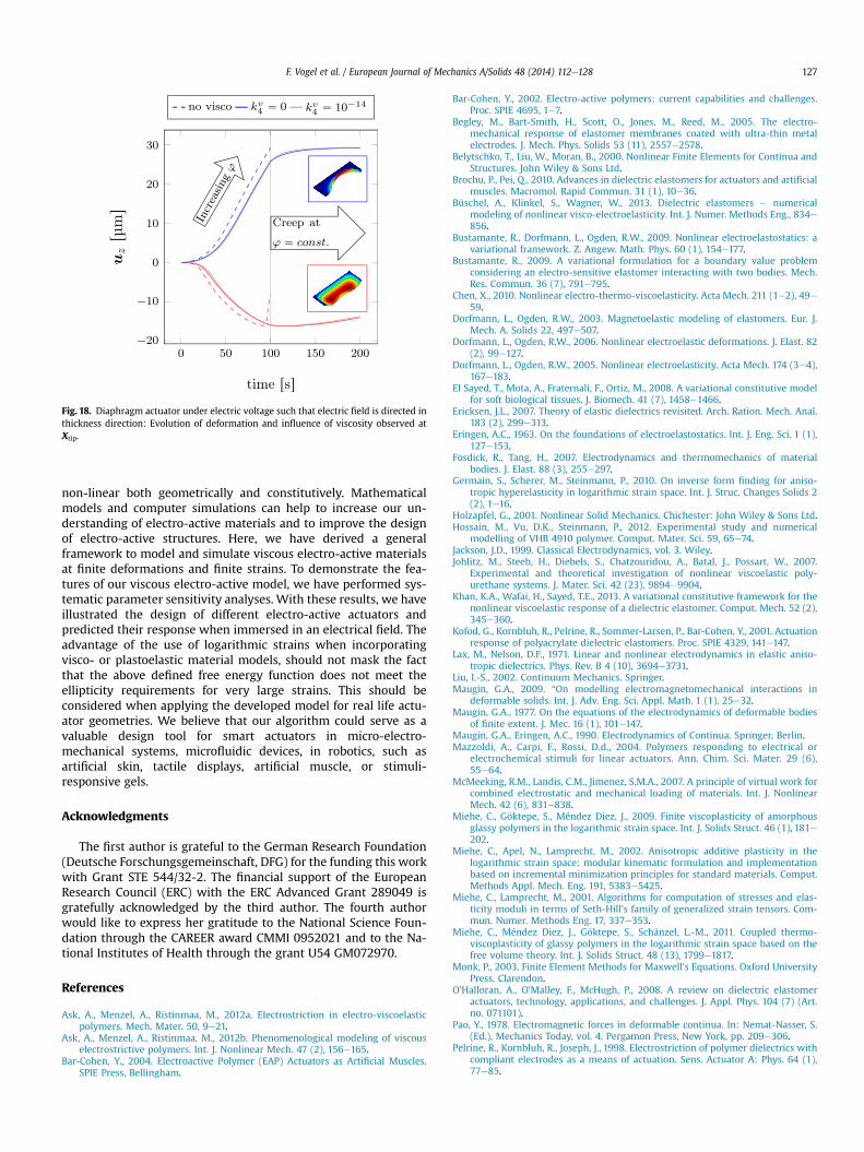
Fig. 18. Diaphragm actuator under electric voltage such that electric field is directed inthickness direction: Evolution of deformation and influence of viscosity observed atXtip.


non-linear both geometrically and constitutively. Mathematicalmodels and computer simulations can help to increase our un-derstanding of electro-active materials and to improve the designof electro-active structures. Here, we have derived a generalframework to model and simulate viscous electro-active materialsat finite deformations and finite strains. To demonstrate the fea-tures of our viscous electro-active model, we have performed sys-tematic parameter sensitivity analyses. With these results, we haveillustrated the design of different electro-active actuators andpredicted their response when immersed in an electrical field. Theadvantage of the use of logarithmic strains when incorporatingvisco- or plastoelastic material models, should not mask the factthat the above defined free energy function does not meet theellipticity requirements for very large strains. This should beconsidered when applying the developed model for real life actu-ator geometries. We believe that our algorithm could serve as avaluable design tool for smart actuators in micro-electro-mechanical systems, microfluidic devices, in robotics, such asartificial skin, tactile displays, artificial muscle, or stimuli-responsive gels.

Acknowledgments

The first author is grateful to the German Research Foundation(Deutsche Forschungsgemeinschaft, DFG) for the funding this workwith Grant STE 544/32-2. The financial support of the EuropeanResearch Council (ERC) with the ERC Advanced Grant 289049 isgratefully acknowledged by the third author. The fourth authorwould like to express her gratitude to the National Science Foun-dation through the CAREER award CMMI 0952021 and to the Na-tional Institutes of Health through the grant U54 GM072970.

References

Ask, A., Menzel, A., Ristinmaa, M., 2012a. Electrostriction in electro-viscoelasticpolymers. Mech. Mater. 50, 9e21.

Ask, A., Menzel, A., Ristinmaa, M., 2012b. Phenomenological modeling of viscouselectrostrictive polymers. Int. J. Nonlinear Mech. 47 (2), 156e165.

Bar-Cohen, Y., 2004. Electroactive Polymer (EAP) Actuators as Artificial Muscles.SPIE Press, Bellingham.

Bar-Cohen, Y., 2002. Electro-active polymers: current capabilities and challenges.Proc. SPIE 4695, 1e7.

Begley, M., Bart-Smith, H., Scott, O., Jones, M., Reed, M., 2005. The electro-mechanical response of elastomer membranes coated with ultra-thin metalelectrodes. J. Mech. Phys. Solids 53 (11), 2557e2578.

Belytschko, T., Liu, W., Moran, B., 2000. Nonlinear Finite Elements for Continua andStructures. John Wiley & Sons Ltd.

Brochu, P., Pei, Q., 2010. Advances in dielectric elastomers for actuators and artificialmuscles. Macromol. Rapid Commun. 31 (1), 10e36.

Büschel, A., Klinkel, S., Wagner, W., 2013. Dielectric elastomers e numericalmodeling of nonlinear visco-electroelasticity. Int. J. Numer. Methods Eng., 834e856.

Bustamante, R., Dorfmann, L., Ogden, R.W., 2009. Nonlinear electroelastostatics: avariational framework. Z. Angew. Math. Phys. 60 (1), 154e177.

Bustamante, R., 2009. A variational formulation for a boundary value problemconsidering an electro-sensitive elastomer interacting with two bodies. Mech.Res. Commun. 36 (7), 791e795.

Chen, X., 2010. Nonlinear electro-thermo-viscoelasticity. Acta Mech. 211 (1e2), 49e59.

Dorfmann, L., Ogden, R.W., 2003. Magnetoelastic modeling of elastomers. Eur. J.Mech. A. Solids 22, 497e507.

Dorfmann, L., Ogden, R.W., 2006. Nonlinear electroelastic deformations. J. Elast. 82(2), 99e127.

Dorfmann, L., Ogden, R.W., 2005. Nonlinear electroelasticity. Acta Mech. 174 (3e4),167e183.

El Sayed, T., Mota, A., Fraternali, F., Ortiz, M., 2008. A variational constitutive modelfor soft biological tissues. J. Biomech. 41 (7), 1458e1466.

Ericksen, J.L., 2007. Theory of elastic dielectrics revisited. Arch. Ration. Mech. Anal.183 (2), 299e313.

Eringen, A.C., 1963. On the foundations of electroelastostatics. Int. J. Eng. Sci. 1 (1),127e153.

Fosdick, R., Tang, H., 2007. Electrodynamics and thermomechanics of materialbodies. J. Elast. 88 (3), 255e297.

Germain, S., Scherer, M., Steinmann, P., 2010. On inverse form finding for aniso-tropic hyperelasticity in logarithmic strain space. Int. J. Struc. Changes Solids 2(2), 1e16.

Holzapfel, G., 2001. Nonlinear Solid Mechanics. Chichester: John Wiley & Sons Ltd.Hossain, M., Vu, D.K., Steinmann, P., 2012. Experimental study and numerical

modelling of VHB 4910 polymer. Comput. Mater. Sci. 59, 65e74.Jackson, J.D., 1999. Classical Electrodynamics, vol. 3. Wiley.Johlitz, M., Steeb, H., Diebels, S., Chatzouridou, A., Batal, J., Possart, W., 2007.

Experimental and theoretical investigation of nonlinear viscoelastic poly-urethane systems. J. Mater. Sci. 42 (23), 9894e9904.

Khan, K.A., Wafai, H., Sayed, T.E., 2013. A variational constitutive framework for thenonlinear viscoelastic response of a dielectric elastomer. Comput. Mech. 52 (2),345e360.

Kofod, G., Kornbluh, R., Pelrine, R., Sommer-Larsen, P., Bar-Cohen, Y., 2001. Actuationresponse of polyacrylate dielectric elastomers. Proc. SPIE 4329, 141e147.

Lax, M., Nelson, D.F., 1971. Linear and nonlinear electrodynamics in elastic aniso-tropic dielectrics. Phys. Rev. B 4 (10), 3694e3731.

Liu, I.-S., 2002. Continuum Mechanics. Springer.Maugin, G.A., 2009. “On modelling electromagnetomechanical interactions in

deformable solids. Int. J. Adv. Eng. Sci. Appl. Math. 1 (1), 25e32.Maugin, G.A., 1977. On the equations of the electrodynamics of deformable bodies

of finite extent. J. Mec. 16 (1), 101e147.Maugin, G.A., Eringen, A.C., 1990. Electrodynamics of Continua. Springer, Berlin.Mazzoldi, A., Carpi, F., Rossi, D.d., 2004. Polymers responding to electrical or

electrochemical stimuli for linear actuators. Ann. Chim. Sci. Mater. 29 (6),55e64.

McMeeking, R.M., Landis, C.M., Jimenez, S.M.A., 2007. A principle of virtual work forcombined electrostatic and mechanical loading of materials. Int. J. NonlinearMech. 42 (6), 831e838.

Miehe, C., Göktepe, S., Méndez Diez, J., 2009. Finite viscoplasticity of amorphousglassy polymers in the logarithmic strain space. Int. J. Solids Struct. 46 (1), 181e202.

Miehe, C., Apel, N., Lamprecht, M., 2002. Anisotropic additive plasticity in thelogarithmic strain space: modular kinematic formulation and implementationbased on incremental minimization principles for standard materials. Comput.Methods Appl. Mech. Eng. 191, 5383e5425.

Miehe, C., Lamprecht, M., 2001. Algorithms for computation of stresses and elas-ticity moduli in terms of Seth-Hill’s family of generalized strain tensors. Com-mun. Numer. Methods Eng. 17, 337e353.

Miehe, C., Méndez Diez, J., Göktepe, S., Schänzel, L.-M., 2011. Coupled thermo-viscoplasticity of glassy polymers in the logarithmic strain space based on thefree volume theory. Int. J. Solids Struct. 48 (13), 1799e1817.

Monk, P., 2003. Finite Element Methods for Maxwell’s Equations. Oxford UniversityPress, Clarendon.

O’Halloran, A., O’Malley, F., McHugh, P., 2008. A review on dielectric elastomeractuators, technology, applications, and challenges. J. Appl. Phys. 104 (7) (Art.no. 071101).

Pao, Y., 1978. Electromagnetic forces in deformable continua. In: Nemat-Nasser, S.(Ed.), Mechanics Today, vol. 4. Pergamon Press, New York, pp. 209e306.

Pelrine, R., Kornbluh, R., Joseph, J., 1998. Electrostriction of polymer dielectrics withcompliant electrodes as a means of actuation. Sens. Actuator A: Phys. 64 (1),77e85.

http://refhub.elsevier.com/S0997-7538(14)00014-X/sref1




























































































































Pelrine, R., Kornbluh, R., Kofod, G., 2000a. High-strain actuator materials based ondielectric elastomers. Adv. Mater. 12 (16), 1223e1225.

Pelrine, R., Kornbluh, R., Pei, Q., Joseph, J., 2000b. High-speed electricallyactuated elastomers with strain greater than 100%. Science 287 (5454),836e839.

Plante, J.-S., Dubowsky, S., 2006. Large-scale failure modes of dielectric elastomeractuators. Int. J. Solids Struct. 43 (25e26), 7727e7751.

Reese, S., Govindjee, S., 1998. A theory of finite viscoelasticity and numerical as-pects. Int. J. Solids Struct. 35, 3455e3482.

Simo, J.C., Hughes, T.J.R., 1998. In: Marsden, J., Sirovich, L., Wiggins, S. (Eds.),Computational Inelasticity. Springer.

Simo, J., Taylor, R., 1985. Consistent tangent operators for rate-independent elas-toplasticity. Comput. Methods Appl. Mech. Eng. 48 (1), 101e118.

Spencer, A., 1971. Theory of invariants. In: Eringen, A.C. (Ed.), Continuum Physics.Academic Press, New York, pp. 239e353.

Steigmann, D.J., 2009. On the formulation of balance laws for electromagneticcontinua. Math. Mech. Solids 14 (4), 390e402.

Steinmann, P., 2011. Computational nonlinear electro-elasticityegetting started:mechanics and electrodynamics of magneto- and electro-elastic materials. In:Ogden, R.W., Steigmann, D.J., CISM Courses and Lectures (Eds.), Mechanics andElectrodynamics of Magneto- and Electro-elastic Materials. Springer, Vienna.

Tiersten, H., 1971. On the nonlinear equations of thermo-electroelasticity. Int. J. Eng.Sci. 9.7, 587e604.

Toupin, R.A., 1956. The elastic dielectric. J. Ration. Mech. Anal. 5, 849e915.Truesdell, C., Toupin, R., 1960. The classical field theories. III/1. In: Flügge (Ed.),

Handbuch der Physik. Springer.Vu, D.K., Steinmann, P., Possart, G., 2007. Numerical modelling of the non-linear

electroelasticity. Int. J. Numer. Methods Eng. 70 (6), 685e704.Wissler, M., Mazza, E., 2007. Electromechanical coupling in dielectric elastomer

actuators. Sens. Actuator A: Phys. 138 (2), 384e393.Wissler, M., Mazza, E., 2005. Modeling of a pre-strained circular actuator made of

dielectric elastomers. Sens. Actuator A: Phys. 120 (1), 184e192.Wriggers, P., 2001. Nichtlineare Finite-Element-Methoden. Springer, Ger. Berlin,

p. 495.

















































european journal of mechanics a/solids - stanford...

Documents