european acceptance scheme - uk performance testing of...

European Acceptance Scheme - UK Performance Testing of EAS GCMS General Survey Test

Final Report to the Drinking Water Inspectorate

EUROPEAN ACCEPTANCE SCHEME - UK PERFORMANCE TESTING OF EAS GCMS GENERAL SURVEY TEST

Final Report to the Drinking Water Inspectorate

Report No: DWI6840

Date: March 2005

Author: H A James

Contract Manager: H A James

Contract No: 14560-0

DWI Reference No: DWI 70/2/172

Contract Duration: November 2004 - March 2005

Any enquiries relating to this report should be referred to the Contract Manager at the following address: WRc-NSF Ltd, Henley Road, Medmenham, Marlow, Bucks, SL7 2HD. Telephone: + 44 (0) 1491 636500 Fax: + 44 (0) 1491 636501

This report has the following distribution: External: DWI - 6 copies + electronic copy; FWR - 2 copies + electronic copy

Internal: Contract manager

CONTENTS Page

1. INTRODUCTION 1

2. OBJECTIVES 3

3. PROGRAMME OF WORK 5

4. RESULTS AND DISCUSSION 7 4.1 Analysis of migration waters 7 4.2 Potential for using the relative response of internal standards to

demonstrate the within-laboratory performance of the method 15 4.3 Analysis of spiked test water samples 23

5. CONCLUSIONS AND RECOMMENDATIONS 39

LIST OF TABLES

Table 4.1 Summary data for migration waters MW1 (from polyethylene pipe) 10 Table 4.2 Summary data for migration waters MW2 (from two component

solvent free epoxy resin) 11 Table 4.3 Summary data for migration waters MW3 (from EPDM rubber) 12 Table 4.4 Within laboratory variation for internal standards (quantification

based on comparison of responses with response for d10-phenanthrene)*. Results from Laboratory A. 16

Table 4.5 Within laboratory variation for internal standards (quantification based on comparison of responses with response for d10-phenanthrene)*. Results from Laboratory B. 18

Table 4.6 Within laboratory variation for internal standards (quantification based on comparison of responses with response for d10-phenanthrene)*. Results from Laboratory C. 20

Table 4.7 Compounds used in performance test exercise and their concentrations in low spike and high spike test waters 24

Table 4.8 Relative GCMS responses of compounds used in spiking solutions 27 Table 4.9 Laboratory A data for spiked samples (µg/l)* 29 Table 4.10 Laboratory B data for spiked samples (µg/l)* 30 Table 4.11 Laboratory C data for spiked samples (µg/l)* 31 Table 4.12 Statistical analysis of Laboratory A data for spiked samples* 32 Table 4.13 Statistical analysis of Laboratory B data for spiked samples 33 Table 4.14 Statistical analysis of Laboratory C for spiked samples 34

LIST OF FIGURES

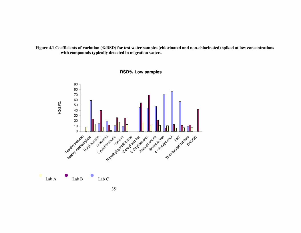
Figure 4.1 Coefficients of variation (%RSD) for test water samples (chlorinated and non-chlorinated) spiked at low concentrations with compounds typically detected in migration waters. 35

Figure 4.2 Coefficients of variation (%RSD) for test water samples (chlorinated and non-chlorinated) spiked at high concentrations with compounds typically detected in migration waters. 36

Figure 4.3 %Bias for test water samples (chlorinated and non-chlorinated) spiked at low concentrations with compounds typically detected in migration waters. 37

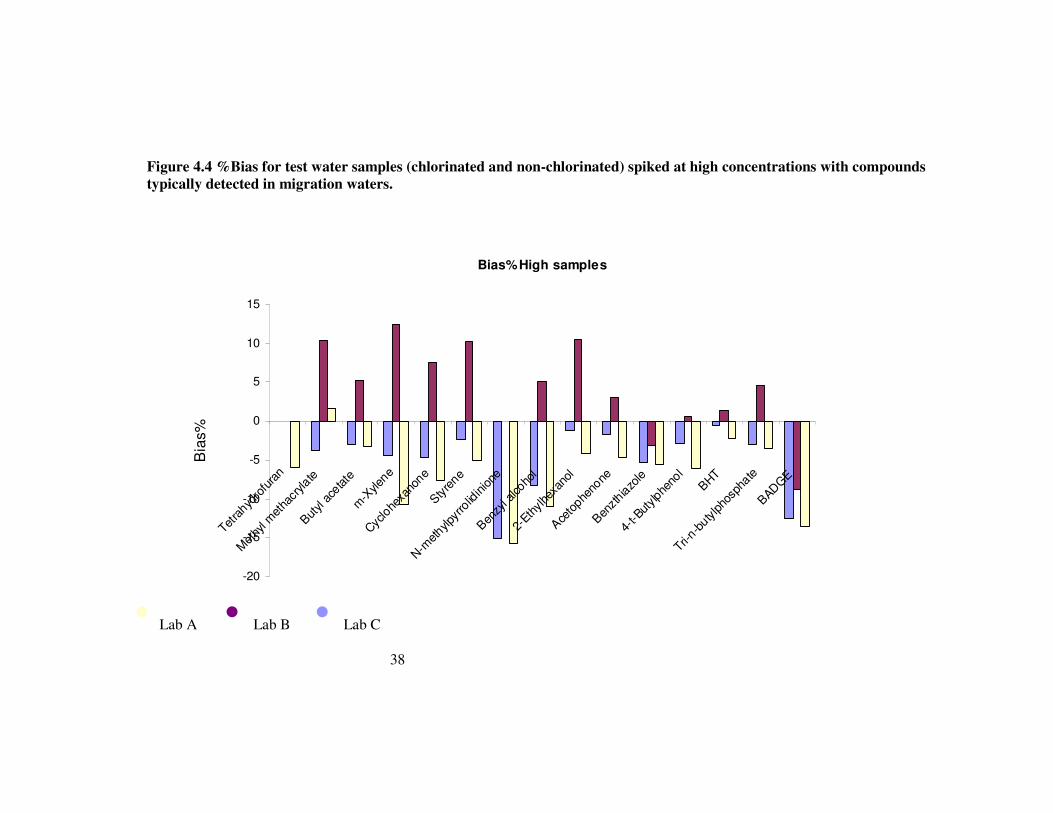
Figure 4.4 %Bias for test water samples (chlorinated and non-chlorinated) spiked at high concentrations with compounds typically detected in migration waters. 38

EXECUTIVE SUMMARY

To reinforce the UK’s case for the inclusion of an analysis using gas chromatography-mass spectrometry (GCMS) to detect unsuspected compounds in migration waters from non-metallic construction products used in contact with public water supplies, the performance of the existing UK test method (BS6920:2001 Part 4) has been assessed by three of the laboratories approved by the UK regulatory body (the Committee on Products and Processes (CPP)). This performance test was supervised by WRc-NSF and the laboratories that participated were WRc-NSF, Law Laboratories and Intertek.

The performance testing exercise had two components. Firstly, three batches of migration waters (unchlorinated and chlorinated) prepared from different products were circulated to the participating laboratories. As the true concentrations of the compounds detected in real migration waters are not known, the results from these samples were used to check the comparability of the data produced by the different laboratories. Each laboratory analysed five samples (test water, chlorinated test water, migration water, chlorinated migration water and a laboratory blank) for each of three products. The second component of the exercise involved an assessment of the semi-quantitative performance of the method, which was checked by analysing samples to which known compounds (fifteen) had been added at known concentrations. Each laboratory analysed three batches of four samples (test water spiked at a low concentration, chlorinated test water spiked at a low concentration, test water spiked at a high concentration, chlorinated test water spiked at a high concentration).

The results from the analysis of real samples indicated that the three laboratories produced broadly comparable data. For two batches of migration waters, all laboratories reported very few compounds at low concentrations. For the other batch of migration waters, where the concentrations of the compounds detected were very high (hundreds of µg l-1), the variation between the highest and lowest concentrations reported for the same compounds by the different laboratories was high (by factors of 2× to 3×). Potential reasons for this variation include the use of different GCMS instruments, GC columns and internal standard solutions by each participant.

By comparing the relative responses of the internal standards (to one of these, d10-phenanthrene), it is possible to determine the relative standard deviations of the responses for eight of the nine internal standards for each batch of migration waters analysed. It is also possible to quantify the remaining standards on the basis of their relative responses compared to d10-phenanthrene, and obtain an indication of the uncertainty of measurement for the overall procedure, as the true concentrations of all of the internal standards are known. It is suggested that each laboratory could maintain a record of their performance on this basis, which may satisfy UKAS’ concerns regarding this method.

The data from the analysis of the spiked test water and spiked chlorinated test water samples containing known compounds at known concentrations indicated that there may be some bias due to chlorination, but this is small in relation to the precision of the analysis. The results from the samples spiked at low concentrations (0.86 – 2.04 µg l-1) confirm that the ability of the approved laboratories to detect and report the presence of

these determinands is relatively good, with two of the participating laboratories reporting the concentrations for thirteen of the compounds present. The compounds that caused problems were tetrahydrofuran (THF), which is very volatile, N-methylpyrrolidinone which is polar and basic and bis-phenolA diglycidyl ether (BADGE) which would normally be determined using a HPLC-based method, rather than GCMS. These three compounds were included in the spiking mixtures because they were known to be “difficult” compounds to analyse using BS6920:2001 Part 4. The results from the samples spiked at high concentrations (8.6 – 20.4 µg l-1) were satisfactory, with variation (% relative standard deviation) being less than 25% for most compounds. The exceptions were the three “difficult” compounds noted earlier. With respect to bias (i.e. the deviation between the reported concentrations and the true concentrations) the results from two laboratories consistently exhibited negative bias, while those from the other laboratory were predominantly positively biased. This may be due to the use of biased internal standard solutions, which could be addressed if internal standard solutions from a single source were available.

The relative GCMS responses of the compounds used in the spiking mixtures was determined by WRC-NSF and, on a per nanogram basis, there was a five-fold variation between the most and least responsive compound (BHT and BADGE, respectively). Given that there is also variation in the responses of the individual internal standards which are used to produce the quantitative estimates of the compounds detected in migration water samples, the results from the spiked samples are better than expected, with the bias for the samples spiked at low concentrations in the range from +150% to –100%, and in the range –20% to +15% for the samples spiked at high concentrations.

Compared to the performance achieved during the EU 5th Framework programme CPDW project, where six of the seven laboratories that participated had no previous experience of applying BS6920:2001 Part 4, the results of this current exercise are an improvement. This suggests that, as expected, experienced users can achieve better performance from the method than inexperienced users, and reinforces the view that following incorporation of this GCMS method into the EAS other European laboratories would be able to utilise the method and obtain similar performance data to the UK laboratories.

It is recommended that:

• the supply of isotopically-labelled internal standards from a single commercial source should be investigated;

• consideration should be given to modifying BS6920:2001 Part 4 to include specifications for the GC column to be used and the temperature programme to be used for the GCMS analysis; additional information on these points will emerge from DG Enterprise-funded work which will commence in April 2005;

• any compounds of interest which have a boiling point lower than that of d6-benzene (79°C) should be analysed as specified compounds using, for example, purge and trap GCMS rather than the procedures specified in BS6920:2001 Part 4.

1

1. INTRODUCTION

One of the analytical requirements of the UK’s regulatory approval scheme for non-metallic construction products used in contact with public water supplies is an analysis using gas chromatography-mass spectrometry (GCMS) used in general survey (investigative) mode. The purpose of this analysis is to detect unsuspected compounds e.g. compounds that may not be declared in the formulation or may be present as impurities in declared substances. The test method is described in BS6920:2001 Part 4.

With minor amendments, the test method has been incorporated into the draft test requirements for the European Acceptance Scheme (EAS) for drinking water construction products. The results of European collaborative research into the GCMS general survey test (EU reports EUR 20833 EN/1 and 20833 EN/2, 2003; Assessment of migration of non-suspected compounds from products in contact with drinking water by GC-MS) indicated that the detection limits achieved were inferior to those obtained in the UK, where the method has been in routine use for many years. At the time it was considered that this was due to the lack of experience of some of the participants in the EU-funded work.

In order to strengthen the UK’s case for the inclusion of the GCMS analytical method in the EAS it is desirable to provide a reliable estimate of detection limits and credible proposals for monitoring the performance of the method. The Drinking Water Inspectorate (DWI) therefore required a scheme to be designed to investigate the inter-laboratory performance of BS6920:2001 Part 4, and for laboratories approved by the UK regulatory body (the Committee on Products and Processes (CPP)) to participate in the performance testing to demonstrate that acceptable performance could be achieved by experienced laboratories.

More recently the one of the UK Accreditation Service’ (UKAS) assessors has raised questions about the adequacy of the internal quality control procedures used by one of the UK test laboratories to monitor the performance of the analytical method. An assessment of the performance of the method, based on the relative responses of the internal standards used in BS6920:2001 Part 4 has been undertaken, to determine whether this approach could be used to address UKAS’ concerns.

Following a tendering process, WRc-NSF were commissioned to design and supervise the exercise, and WRc-NSF, Law Laboratories and Intertek (all of whom are currently CPP designated test laboratories) were chosen to participate in the inter-laboratory performance testing. This report describes the work undertaken, the results obtained and an assessment of their significance. The results from the participating laboratories are presented as originating from laboratory A, B or C; these designations have been randomly applied.

3

2. OBJECTIVES

The objectives of the work involved with respect to the design and supervision of the inter-laboratory scheme were as follows:

1. To propose a scheme of analysis and timetable for distribution of standard solutions for a maximum of four test laboratories in order to characterise the inter-laboratory performance of BS6920:2001 Part 4.

2. To propose a procedure involving analysis of a representative selection of test substances that will provide a reliable check on the maintenance of acceptable performance of the method under conditions of routine analysis.

3. To supervise the inter-laboratory trial, to provide instructions and distribute samples to participants, to advise as necessary on the testing, and to provide a final report on the outcome of the testing that includes detailed proposals for routine monitoring of the performance of the method of analysis.

4. If required, to devise a procedure to check on the quantitative performance of the method for compounds which are typically found in migration waters from materials submitted for approval.

5. To ensure that the participants adhere to the agreed timetables for conduct of the study and the reporting of the results.

The objectives of the work involved in respect of participation in the inter-laboratory scheme were as follows:

6. To carry out analysis to BS6920:2001 Part 4, following instructions provided by the co-ordinating contractor on up to 12 samples of migration waters, test waters and associated laboratory blanks, and to report the results of the analysis to the co-ordinating laboratory within the agreed timescale.

7. To analyse to BS6920:2001 Part 4 additional samples, up to a maximum of eight samples.

8. To provide written comments and reports in a format requested by the co-ordinator.

5

3. PROGRAMME OF WORK

Although it would have been possible to devise a performance test using only water samples to which a variety of compounds identified during previous materials testing work had been added, it was considered that the testing would be more credible if real migration waters were used. Therefore the work programme devised involved the analysis of both spiked samples and migration waters prepared from non-metallic products.

As the true concentrations of the compounds detected in real migration waters are not known, the results from these samples would be used to check on the comparability of the data produced by the different approved laboratories, but no information would be available with respect to the quantitative accuracy of the results. This latter point could only be addressed by analysing samples to which known compounds had been added at known concentrations. Therefore spiking solutions that contained fifteen compounds previously detected in migration waters from non-metallic materials were prepared and circulated to the participating laboratories. Participants were instructed to spike an appropriate amount of these solutions (100 µl) into their own test waters (chlorinated and non-chlorinated) and conduct the analysis according to BS6920:2001 Part 4. One of the solutions, the low spike, contained the various chosen compounds at concentrations such that their concentrations in the samples analysed were in the range 0.86-2.04 µg l-1; the other spiking solution, the high spike, was ten times more concentrated so that the concentrations in the samples analysed were in the range 8.6-20.4 µg l-1. Three batches of spiked samples (low spike in non-chlorinated test water; low spike in chlorinated test water; high spike in non-chlorinated test water; high spike in chlorinated test water) were analysed.

For the analysis of real migration waters, WRc-NSF produced sufficient quantities of migration water (chlorinated and non-chlorinated; migration waters after the third 72-hour leaching period) from each of three non-metallic materials, together with the test water used (chlorinated and non-chlorinated), so that each participating laboratory received identical samples for analysis. These were delivered to each participating laboratory by noon on a specified date, on the day following sampling. Each laboratory was instructed to begin the analysis (i.e. extract the samples) on the afternoon of sample receipt. Thus each laboratory analysed three batches of four samples (non-chlorinated test water, chlorinated test water, non-chlorinated migration water and chlorinated migration water). A laboratory blank was also analysed for each batch. In total, each laboratory analysed fifteen samples.

The alternative to the preparation and circulation of the migration waters by the organising laboratory would have been to supply each laboratory with samples of the various materials so that they could prepare their own migration waters for analysis. However this could have introduced variability from the materials themselves (as not all of the samples would necessarily be identical) and from the preparation of the migration waters (e.g. slightly different temperatures and/or times), so the overall variability would no longer be due to only the analysis.

6

The actual timescale for the work was as follows:

Meeting of representatives from the participating laboratories and the organising laboratory at DWI: 10 November 2004.

Migration water (MW1) samples circulated: 7 December 2004

Migration water (MW2) samples circulated: 21 December 2004

Migration water (MW3) samples circulated: 11 January 2005

Spiking solutions circulated: 16 December 2004

7

4. RESULTS AND DISCUSSION

4.1 Analysis of migration waters

The results obtained for the migration water samples (MW1, MW2 and MW3) by each laboratory are summarised in Tables 4.1, 4.2 and 4.3 below, and are given in full in Appendix 1.

The GCMS systems used by each laboratory were as follows:

WRc-NSF – VG 70E (magnetic) mass spectrometer, HP5980 Series II GC (on-column injector) with J&W DB-1 60m (0.32 mm ID; 0.25 µm film thickness) capillary column.

Law Laboratories – Hewlett-Packard 5972 MSD (quadrupole) mass spectrometer, HP5890 Series II GC (on-column injector) with Restek Rtx-1 60m (0.32 mm ID; film thickness 0.25 µm) capillary column.

Intertek – Perkin Elmer Clarus 500 (quadrupole) mass spectrometer, Clarus 500 GC with J&W DB-1 60m (0.32 mm ID; film thickness 0.25 µm) capillary column.

The products used to prepare the migration waters were as follows:

for migration waters 1 (MW1) – polyethylene pipe;

for migration waters 2 (MW2) – two component solvent free epoxy resin;

for migration waters 3 (MW3) – EPDM rubber.

The migration waters were prepared according to EN 12873-1 (MW1 and MW3) and EN 12873-2 (MW2). In essence both procedures involved an initial rinsing or pre-washing of the product, followed by three stagnation periods of 72 hours with the test water. Separate samples were treated identically, but chlorinated test water was used to prepare the chlorinated migration waters. Prior to distributing the chlorinated migration waters to the participating laboratories for analysis, they were de-chlorinated according to BS6920:2001 Part 4 (using an aqueous solution of ascorbic acid).

As noted earlier, each laboratory analysed samples of test water, chlorinated test water, migration water and chlorinated migration water, together with a laboratory blank, for each product.

For the migration waters from the polyethylene pipe, it can be seen from Table 4.1 that few compounds were detected and the concentrations reported were generally low (< 5 µg l-1). Laboratory A only reported two compounds at a concentration above 1 µg l-1, and the highest concentration reported was an unknown present at 2.4 µg l-1. Laboratory B reported three compounds above 1 µg l-1 in the migration water sample and four compounds present above 1 µg l-1 in the chlorinated migration water sample. In total four

8

of the compounds detected were reported as unknown, but in each case they were only detected by one laboratory, and the highest concentration reported for any of the unknowns was 2.4 µg l-1.

For the migration waters from the two component solvent free epoxy resin, again few compounds were detected above 1 µg l-1 (Table 4.2) with the highest concentration reported being 1.7 µg l-1 for an unknown. Laboratory A did not detect any compounds at a concentration > 1 µg l-1 in either the migration water or chlorinated migration water samples, while laboratories B and C detected one compound in the migration water sample and two compounds in the chlorinated migration water sample.

The results from the migration waters from the EPDM rubber showed that, in complete contrast to the MW1 and MW2 samples, many compounds were detected by all three laboratories at very high (>100 µg l-1) concentrations. However of the 56 compounds detected at concentrations > 1µg l-1, only 14 were identified, and 19 compounds were only reported by one laboratory (i.e. not reported by the other two laboratories; 2 compounds were only detected by laboratory A, two only by laboratory B and the remaining 15 only by laboratory C). Some difficulties were encountered in drawing up a summary table of all of the data (Table 4.3) as it was not always possible to be certain which of the unknown compounds reported by the different laboratories were in fact the same compound as an unknown reported by another laboratory. Where compounds were reported at high concentrations (> 50 µg l-1) it was possible to be fairly certain, even for unknowns, that the same compound was being reported by all three laboratories.

The problem with the correlation of data relating to unknowns from different laboratories arises partly because BS6920:2001 Part 4 does not specify the GC column to be used for the GCMS analysis, nor does it specify the GC temperature programme to be used. At the time this standard was written, it was not considered desirable for it to be too prescriptive in this respect. However if the comparison of data from different laboratories becomes important (e.g. for audit purposes), it may be necessary to be more specific and insist on the use of particular GC columns under defined conditions. Further work on this aspect of the overall analysis forms part of a proposal submitted to DG Enterprise for further R&D work aimed at incorporating GCMS into the EAS. It is understood that the work is likely to be funded and will probably commence in April 2005, but at present no official confirmation of this start date has been received.

In terms of the quantities of the various compounds reported (identified and unknowns), there was considerable variation for compounds detected at high concentrations. For example, in the case of 2-(2-butoxyethoxy)ethanol, the concentrations reported were in the range 294-990 µg l-1 for the migration waters and in the range 240-870 µg l-1 for the chlorinated migration waters. For benzthiazole the ranges reported were 78-286 µg l-1 and 107-394 µg l-1 and for 2-mercaptobenzthiazole the ranges were 424-645 µg l-1 and 283-495 µg l-1 respectively. For compounds detected at lower concentrations, the variability was similar (in % terms). For example dibutylformamide was reported in the range 11-31 µg l-1 in the migration waters and in the range 12-35 µg l-1 in the chlorinated migration waters.

Undoubtedly some of the variability in the reported concentrations for compounds

9

detected at high levels is due to the fact that the GCMS systems used were set up to detect compounds present in migration waters at concentrations above 1 µg l-1. Depending on the dynamic range of the data system used to acquire and process the mass spectral data the response in terms of total ion current (TIC) peak areas will, at a certain concentration (which will be compound dependent), become non-linear. As different GCMS systems were used by the participating laboratories, it is therefore not surprising that at very high concentrations there is considerable variation.

Another factor that could well be contributing to the inter-laboratory variability is the potential variability in the mixture of the isotopically-labelled internal standards used by each laboratory to spike all samples analysed. This mixture is made up independently by each laboratory from nine individual pure standards. Initially individual stock solutions are prepared, from which a mixed intermediate solution is prepared by dilution. A further dilution of the intermediate solution gives the internal standards spiking solution. There will be errors associated with all of these steps, so some variation is inevitable. One way of addressing this, and therefore reducing inter-laboratory variation, would be for each laboratory to use identical solutions of internal standards. Several commercial suppliers of pure analytical standards additionally offer to supply customer-specified mixed solutions of standards. It may be worthwhile approaching one or more of these companies to establish whether they would be prepared to supply suitable solutions (one for use as the GC column test solution and the other for use as the internal standards spiking solution), and the likely costs involved. However, because of the relatively low demand (four CPP approved laboratories in the UK), the costs are likely to be high.

In spite of the variability of the results reported by each laboratory there is little doubt that regardless of which data set was being considered, the presence of so many compounds (identified and unknown) at the concentrations reported would result in serious concerns regarding the suitability of the product used to prepare the MW3 migration waters for use in contact with drinking water, unless the conditions of use meant that the concentrations encountered by drinking water consumers would be several orders of magnitude lower than those detected in the leach test.

10

Table 4.1 Summary data for migration waters MW1 (from polyethylene pipe)*

Compounds detected above 1.0 µg/l Unchlorinated migration water Chlorinated migration water Lab. A Lab. B Lab. C Lab. A Lab. B Lab. C Dimethylsuccinate <1 1.0 1.8 <1 <1 1.8 Acetophenone ND ND 1.9 ND ND ND 7,9-Di-t-butyl-1-oxaspiro[4.5]deca-6,9-diene-2,8-dione

ND ND 2.7 ND ND 4.6

Di-isobutyl phthalate 2.0 2.8 ND 2.2 4.6 ND Di-n-butyl phthalate ND 1.0 ND ND 1.6 ND Unknown (57, 164, 41, 179) ND ND ND ND 1.0 ND Unknown (43, 151, 41, 125) ND ND ND ND 1.8 ND Unknown (44, 41, 57, 217) 1.9 ND ND 2.4 ND ND Unknown (43, 125, 151, 300) ND ND ND ND ND 1.3

*ND - not detected

11

Table 4.2 Summary data for migration waters MW2 (from two component solvent free epoxy resin)*

Compounds detected above 1.0 µg/l Unchlorinated migration water Chlorinated migration water Lab. A Lab. B Lab. C Lab. A Lab. B Lab. C Propoxybutane ND ND ND ND 1.1 ND Unknown (83, 41, 56, 126) ND ND ND ND 1.1 ND Unknown (140, 155, 72, 83) <1 ND 1.0 <1 ND 1.0 Unknown (83, 56, 126, 155) ND ND ND <1 ND 1.7 Decanamine ND 1.5 ND ND ND ND

*ND – not detected

12

Table 4.3 Summary data for migration waters MW3 (from EPDM rubber)*

Compounds detected above 1.0 µg/l Unchlorinated migration water Chlorinated migration water Lab. A Lab. B Lab. C Lab. A Lab. B Lab. C 2-Butoxyethanol 1.3 ND 2.6 1.8 ND 3.7 Unknown (59, 57, 41, 43) 1.0 ND ND 2.0 ND ND Isothiocyanatobutane ND ND 7.1 ND ND 5.3 Acetophenone 1.2 1.8 1.2 1.0 1.7 1.0 2-Phenyl-2-propanol 1.8 3.0 ND 1.6 3.9 ND Unknown (29, 42, 56, 115) 14.0 4.6 10.4 16.0 24.0 10.2 Unknown (57, 27, 41, 45) 7.2 5.1 ND 21.0 22.0 ND 2-(2-butoxyethoxy)ethanol 294.0 990.0 360.3 240.0 870.0 298.6 Benzthiazole 78.0 286.0 103.6 107.0 394.0 138.7 Unknown 70, 114, 43 ND ND 3.5 ND ND 3.7 Dibutylformamide 15.0 31.0 11.4 16.0 35.0 11.6 Unknown (70, 114, 57, 29) 4.6 4.5 4.5 5.9 12.0 5.4 Unknown (57, 29, 41, 45) 27.0 164.0 35.8 13.0 79.0 17.8 Unknown (43, 109, 41, 151) 1.3 7.2 ND 1.1 3.2 ND Unknown (57, 45, 41, 29) 16.0 51.0 19.3 17.0 54.0 20.8 Di-t-butylphenol isomer ND ND 3.5 ND ND 4.6 Unknown (86, 130, 43, 45) 4.1 6.5 6.3 4.9 5.7 6.1 Unknowns (43, 135, 177, 57) + (57, 29, 41, 156) 1.2 3.5 ND 1.8 1.7 3.5 Unknown (86, 130, 29, 27) 14.2 32.0 13.7 12.0 27.0 11.8 2-Methylthiobenzthiazole 2.2 3.2 ND <1 2.6 ND

13

Table 4.3 Summary data for migration waters MW3 (from EPDM rubber)* (continued) Unknown (86, 72, 60, 29) 17.0 8.7 14.0 6.7 2-Hydroxybenzthiazole

18.0 17.0 13.9

14.0 17.0 17.4

Unknown (169, 168, 167) + p-Tolylpyridine ND ND 8.7 ND ND 2.9 Unknown (70, 114, 169) ND ND 5.0 ND ND 5.6 Unknowns (100, 44, 72, 29) + (57, 45, 29, 41) 4.2 2.8 3.9 5.7 4.7 3.9 Unknown (44, 45, 100, 133) ND 1.2 3.4 ND 3.8 4.0 Unknown (114, 57, 70, 29) 3.8 6.6 3.9 5.7 7.3 4.7 Unknown (180, 215, 108) ND ND 3.3 ND ND 2.6 Unknown (45, 89, 218) ND ND 3.2 ND ND 4.7 Dibutyl phthalate ND ND 2.1 ND ND ND 7,9-Di-t-butyl-1-oxaspiro(4,5)deca-6,9-diene-2,8-dione

ND ND 1.2 ND ND ND

Unknown (45, 29, 57, 41) ND 2.8 ND 2.0 6.2 ND Unknown (86, 130, 216, 27) 1.5 ND 12.7 2.6 4.3 11.6 2-Mercaptobenzthiazole 424.0 645.0 329.5 483.0 495.0 282.5 Unknown (163, 135, 220, 162) 136.0 218.0 161.9 168.0 234.0 177.8 Unknown (57, 29, 41, 45) 94.0 540.0 189.0 279.0 698.0 435.2 Unknown (29, 103, 59, 87) 12.0 66.0 47.3 36.0 74.0 40.8 Unknown (167, 45) ND ND 1.8 ND ND 2.7 Unknown (86, 130, 70, 244) 2.0 12.0 3.6 1.6 10.0 ND Unknown (86, 167, 130, 70) 2.0 2.2 1.0 4.3 2.5 ND Unknown (86, 135, 162, 134) 17.0 21.0 16.3 20.0 26.0 19.2 Unknown (45, 57, 29, 103) <1 ND ND 1.1 ND ND Unknown (86, 56, 135, 29) 6.4 9.3 16.3 8.1 14.0 ND Unknown (86, 260, 130, 27) 7.4 11.0 8.2 5.5 8.2 7.3

14

Table 4.3 Summary data for migration waters MW3 (from EPDM rubber)* (continued) Unknown (166, 57, 41, 194) ND ND 31.6 ND ND 33.2 Unknown (179, 86, 264, 135) 4.6 7.0 7.0 3.8 7.0 6.5 Di(2-ethylhexyl) phthalate ND ND 23.5 ND ND 4.9 Unknown (167, 211) ND ND 2.5 ND ND 2.9 Unknown (57, 55, 129, 45) ND 8.2 ND 1.3 9.2 ND Unknown (57, 45, 41, 29) ND 14.0 ND 4.4 12.0 ND Unknown (100, 194, 72, 29) ND 1.8 ND ND ND ND Unknown (129, 57, 86, 198) ND ND 3.2 ND ND 6.5 Unknown (57, 101, 45, 41) ND ND 9.1 ND 17.0 28.8 Unknown (300, 242, 108, 69) 3.4 12.0 12.2 17.0 32.0 14.4 Unknown (194, 57, 41, 29) ND 11.5 ND ND 6.3 ND Unknown (180, 167, 136) ND ND 4.0 ND ND ND

*ND – not detected

15

4.2 Potential for using the relative response of internal standards to demonstrate the within-laboratory performance of the method

Because the actual concentrations of the various compounds present in the migration -water samples analysed was not known, it was proposed that the within-laboratory variation of the overall procedure would be assessed by using one of the isotopically-labelled internal standards (d10-phenanthrene) to quantify the remaining internal standards. A further reason for undertaking this exercise was to establish whether this approach could provide the basis of a procedure that would be acceptable to UKAS for demonstrating that the overall procedure applied was “in control” for each analytical batch, and to provide some estimate of uncertainty associated with the overall analysis, so as to minimise any additional analytical effort. The results of this exercise are given in Tables 4.4 – 4.6.

For the batches from the migration waters produced from the two materials where few compounds were detected at low concentrations (MW1 and MW2), all of the results are comparable i.e. the within-laboratory variation is generally less than 20%, with the exception of d6-benzene, the most volatile internal standard, and the one most likely to be lost during the concentration step after the solvent extraction and prior to the GCMS analysis. For the migration waters that contained many compounds, some of which were present at high concentrations (MW3), the variability is generally poorer although for one laboratory (laboratory B) this effect was not as marked. The other two laboratories were unable to quantify the peak for one of the internal standards (d8-naphthalene) because it co-eluted with one of the compounds that leached from the material, and one of these (laboratory C) experienced similar problems with the quantification of d5-phenol. This is probably due be due to the different GC columns used – laboratories A and C used the same GC column, while laboratory B used a different GC column. As noted earlier, the standardisation of the GC column and GC conditions will be the subject of future R&D work.

On the basis of these data it should be possible to use the variability of the response of, say, three or four of the internal standards compared to d10-phenanthrene to establish that the overall method is “in control” e.g. the within-batch variability could be checked, and if <20% then the performance of the method would be considered acceptable.

In terms of uncertainty of the quantification, a statistical analysis of laboratory A’s data for the internal standards indicates that using d10-phenanthrene to quantify the remaining internal standards provides results that are generally within a factor of ×2 to ×3 of the known concentrations. For example, the average concentration of d6-benzene for the three batches of migration waters analysed is 0.79 µg l-1, when the true value is 2.00 µg l-

1. For d5-chlorobenzene, the respective numbers are 1.44 µg l-1 and 2.0 µg l-1, and for d20-BHT they are 8.9 µg l-1 and 7.09 µg l-1. Each laboratory could determine its own estimate of uncertainty in this way and by maintaining control charts again demonstrate that the method is “in control”

16

Table 4.4 Within laboratory variation for internal standards (quantification based on comparison of responses with response for d10-phenanthrene)*. Results from laboratory A.

MW1 Internal standard Lab. Blank TW TWCl MW MWCl Mean SD CV% d6-Benzene 0.9 0.5 0.6 0.5 0.7 0.64 0.17 26.1 d5-Chlorobenzene 1.5 1.1 1.2 1.1 1.0 1.18 0.19 16.3 d10-p-Xylene 1.1 0.9 0.9 0.9 0.7 0.90 0.14 15.7 d5-Phenol 0.9 0.7 0.8 0.8 0.8 0.80 0.07 8.8 d8-Naphthalene 1.1 0.9 0.9 0.9 0.9 0.94 0.09 9.5 d20-BHT 6.4 5.7 6.1 5.5 6.4 6.02 0.41 6.8 d34-Hexadecane 1.8 1.5 1.6 1.5 1.6 1.60 0.12 7.7 d10-Phenanthrene 2.0 2.0 2.0 2.0 2.0 2.00 0.00 0.0 d62-Squalane 7.2 6.0 7.1 7.2 8.3 7.16 0.81 11.4

MW2 Internal standard Lab. Blank TW TWCl MW MWCl Mean SD CV%

d6-Benzene 0.9 0.9 0.9 0.8 0.8 0.86 0.05 6.4 d5-Chlorobenzene 1.7 1.8 1.4 1.4 1.3 1.52 0.22 14.3 d10-p-Xylene 1.2 1.3 1.1 1.0 1.0 1.12 0.13 11.6 d5-Phenol 1.0 1.2 0.9 0.9 0.9 0.98 0.13 13.3 d8-Naphthalene 1.2 1.3 1.1 1.0 1.2 1.16 0.11 9.8 d20-BHT 6.9 7.7 6.5 6.5 6.0 6.72 0.63 9.4 d34-Hexadecane 1.6 1.7 1.5 1.5 1.4 1.54 0.11 7.4 d10-Phenanthrene 2.0 2.0 2.0 2.0 2.0 2.00 0.00 0.0 d62-Squalane 4.9 5.0 4.8 4.3 4.3 4.66 0.34 7.2

17

Table 4.4 (continued)

MW3

Internal standard Lab. Blank TW TWCl MW MWCl Mean SD CV%

d6-Benzene 0.9 0.9 0.9 0.8 0.8 0.86 0.05 6.4 d5-Chlorobenzene 1.7 1.6 1.7 1.5 1.6 1.62 0.08 5.2 d10-p-Xylene 1.2 1.2 1.2 1.1 1.2 1.18 0.04 3.8 d5-Phenol 1.1 1.2 1.2 0.4 0.4 0.86 0.42 49.1 d8-Naphthalene 1.2 1.5 1.5 NQ NQ NC NC NC d20-BHT 7.2 7.3 7.4 9.5 10.1 8.30 1.39 16.7 d34-Hexadecane 1.6 1.6 1.6 1.2 1.9 1.58 0.25 15.8 d10-Phenanthrene 2.0 2.0 2.0 2.0 2.0 2.00 0.00 0.0 d62-Squalane 2.1 2.2 2.4 11.3 13.0 6.20 5.47 88.2

NQ – not quantified, due to interference NC – not calculated

* TW = test water TWCl = chlorinated test water MW = migration water MWCl = chlorinated migration water SD = standard deviation CV% = coefficient of variation (relative standard deviation expressed as a percentage)

18

Table 4.5 Within laboratory variation for internal standards (quantification based on comparison of responses with response for d10-phenanthrene)*. Results from laboratory B.

MW1 Internal standard Lab. Blank TW TWCl MW MWCl Mean SD CV% d6-Benzene 0.5 0.4 0.4 0.3 0.6 0.44 0.11 25.9 d5-Chlorobenzene 0.9 0.8 0.7 0.6 0.7 0.74 0.11 15.4 d10-p-Xylene 0.5 0.5 0.4 0.3 0.4 0.42 0.08 19.9 d5-Phenol 2.0 1.7 1.5 1.3 1.8 1.66 0.27 16.3 d8-Naphthalene 0.8 0.7 0.7 0.5 0.6 0.66 0.11 17.3 d20-BHT 7.9 5.9 6.7 5.0 7.5 6.60 1.18 17.9 d34-Hexadecane 1.0 0.7 0.8 0.6 0.9 0.80 0.16 19.8 d10-Phenanthrene 2.0 2.0 2.0 2.0 2.0 2.00 0.00 0.0 d62-Squalane 10.5 8.2 9.9 5.9 9.9 8.88 1.87 21.1 MW2

Internal standard Lab. Blank TW TWCl MW MWCl Mean SD CV% d6-Benzene 0.5 0.4 0.2 0.3 0.2 0.32 0.13 40.7 d5-Chlorobenzene 2.3 2.7 1.4 1.6 1.5 1.90 0.57 30.0 d10-p-Xylene 0.7 0.7 0.5 0.6 0.4 0.58 0.13 22.5 d5-Phenol 1.2 1.6 1.0 1.1 1.4 1.26 0.24 19.1 d8-Naphthalene 0.8 0.8 0.6 0.8 0.6 0.72 0.11 15.2 d20-BHT 8.6 8.8 6.2 7.3 6.2 7.42 1.25 16.9 d34-Hexadecane 1.0 1.2 0.8 1.0 0.8 0.96 0.17 17.4 d10-Phenanthrene 2.0 2.0 2.0 2.0 2.0 2.00 0.00 0.0 d62-Squalane 11.6 12.0 10.6 12.5 9.1 11.16 1.35 12.1

19

Table 4.5 Continued

MW3 Internal standard Lab. Blank TW TWCl MW MWCl Mean SD CV% d6-Benzene 0.7 0.9 1.0 0.8 0.7 0.82 0.13 15.9 d5-Chlorobenzene 1.7 1.5 1.4 1.2 1.0 1.36 0.27 19.9 d10-p-Xylene 0.9 0.9 0.8 0.6 0.5 0.74 0.18 24.5 d5-Phenol 2.7 1.7 1.5 1.8 1.7 1.88 0.47 25.1 d8-Naphthalene 1.0 1.0 1.0 0.7 0.8 0.90 0.14 15.7 d20-BHT 7.5 7.3 7.4 6.9 6.5 7.12 0.41 5.8 d34-Hexadecane 1.3 1.4 1.5 1.4 1.0 1.32 0.19 14.6 d10-Phenanthrene 2.0 2.0 2.0 2.0 2.0 2.00 0.00 0.0 d62-Squalane 11.1 11.1 12.2 12.4 11.5 11.66 0.61 5.2


20

Table 4.6 Within laboratory variation for internal standards (quantification based on comparison of responses with response for d10-phenanthrene)*. Results from laboratory C.

MW1 Internal standard Lab. Blank TW TWCl MW MWCl Mean SD CV% d6-Benzene 0.2 0.2 0.3 0.2 0.3 0.24 0.05 22.8 d5-Chlorobenzene 0.4 0.3 0.3 0.3 0.3 0.32 0.04 14.0 d10-p-Xylene 0.4 0.3 0.4 0.3 0.4 0.36 0.05 15.2 d5-Phenol 1.3 0.9 1.2 0.9 1.1 1.08 0.18 16.6 d8-Naphthalene 0.8 0.7 0.7 0.8 0.8 0.76 0.05 7.2 d20-BHT 6.2 4.7 5.6 4.5 5.5 5.30 0.70 13.1 d34-Hexadecane 0.8 0.7 0.8 0.6 0.7 0.72 0.08 11.6 d10-Phenanthrene 2.0 2.0 2.0 2.0 2.0 2.00 0.00 0.0 d62-Squalane 7.1 5.3 6.5 4.5 6.5 5.98 1.05 17.6 MW2 Internal standard Lab. Blank TW TWCl MW MWCl Mean SD CV% d6-Benzene 0.3 0.2 0.2 0.3 0.2 0.24 0.05 22.8 d5-Chlorobenzene 0.8 0.9 0.5 0.5 0.4 0.62 0.22 35.0 d10-p-Xylene 0.4 0.4 0.3 0.4 0.3 0.36 0.05 15.2 d5-Phenol 1.2 0.9 1.0 1.0 0.9 1.00 0.12 12.2 d8-Naphthalene 0.8 0.6 0.7 0.6 0.6 0.66 0.09 13.6 d20-BHT 5.7 5.1 4.5 5.4 3.6 4.86 0.83 17.1 d34-Hexadecane 1.2 1.0 1.0 1.1 0.9 1.04 0.11 11.0 d10-Phenanthrene 2.0 2.0 2.0 2.0 2.0 2.00 0.00 0.0 d62-Squalane 6.8 6.8 5.1 6.2 5.4 6.06 0.79 13.0

21

Table 4.6 Continued

MW3 Internal standard Lab. Blank TW TWCl MW MWCl Mean SD CV% d6-Benzene 0.2 0.3 0.2 0.1 0.1 0.18 0.08 46.5 d5-Chlorobenzene 1.5 1.3 1.1 0.4 0.6 0.98 0.47 47.5 d10-p-Xylene 0.5 0.4 0.4 0.2 0.2 0.34 0.13 39.5 d5-Phenol 1.6 1.3 1.1 NQ NQ NC NC NC d8-Naphthalene 0.8 0.7 0.7 NQ NQ NC NC NC d20-BHT 6.4 5.4 4.9 3.0 4.0 4.74 1.30 27.5 d34-Hexadecane 1.4 1.3 1.2 0.5 0.7 1.02 0.40 38.8 d10-Phenanthrene 2.0 2.0 2.0 2.0 2.0 2.00 0.00 0.0 d62-Squalane 7.3 6.2 5.5 2.7 3.5 5.04 1.90 37.8 NQ – not quantified, due to interference NC – not calculated


23

4.3 Analysis of spiked test water samples

The purpose of analysing test water samples spiked at low and high concentrations with fifteen compounds (all of which have previously been identified in various migration waters from materials intended to be used in contact with drinking water) was to establish the typical quantitative accuracy of the results obtained.

It should be borne in mind that the application of the BS6920:2001 Part 4 method to a migration water sample does not guarantee that all organic compounds leached from materials will be detected and accurately quantified. No currently available analytical technique will accomplish this, but the general survey GCMS approach provides a cost-effective way of detecting and identifying many of the compounds that could be present in migration waters, and allows an estimate of their concentration to be made. If accurate quantitative results are required then specific methods optimised for the compounds of interest should be applied. However given the range of compounds which could potentially be present (either intentionally or unintentionally) in migration waters it is not realistic either in terms of the numbers of specific methods that would need to be applied, or in terms of the timescales and costs, to conduct numerous specific analyses. General survey GCMS analysis is therefore a compromise, and it has to be accepted that there are some shortcomings with this approach.

For a compound to be detected it must, first of all, be extracted from the migration water sample under the conditions specified in BS6920:2001 Part 4. Neutral organic compounds are not particularly water soluble and can be extracted efficiently using liquid-liquid extraction with dichloromethane. Polar organic compounds are more water soluble and are extracted less efficiently, while compounds that are ionised in aqueous solution will be poorly extracted (if at all). The extraction efficiencies of polar or ionic compounds can be maximised by adjusting either the pH of the water sample or the ionic strength (a procedure sometimes referred to as “salting out”) of the sample.

Assuming a compound has been successfully extracted, it is also necessary for it to be amenable to GCMS analysis for it to be detected and quantified. Generally organic (or organometallic compounds) with boiling points between 60°C and about 500°C can be detected using GCMS as described in BS6920:2001 Part 4. This does mean that some compounds present in CPDW materials (e.g. antioxidants with molecular weights >700) cannot be detected (although some of their breakdown products may be). Again this means that such compounds, if they are of concern, must be determined using appropriate specific optimised methods.

As noted above, the primary purpose of the GCMS analysis is the detection and identification of unsuspected compounds present in migration waters. The semi-quantitative information that is obtained for the compounds detected is based on a comparison of their responses (TIC chromatogram peak areas) with those of the internal standards. For a compound which is similar to an internal standard (in terms of extraction efficiency and GCMS response) it would be expected that this method of quantifying would provide an approximation of the real quantity present. However for the various reasons given above, for some compounds this may provide a significant under-estimate

24

of their true concentration.

When choosing the compounds to be used to check on the quantitative performance of the overall method it would have been possible to select fifteen compounds that were not amenable to the method (e.g. were very poorly extracted and were of high molecular weight). However this would not have led to the production of useful data. Therefore the compounds chosen were representative of the types of compounds that have been detected in the past in migration waters from a variety of products. They are listed in Table 4.7 below, together with their concentrations when used to produce spiked samples at low and high concentrations.

The mixed spiking solutions were made up from individual solutions of pure standards and separate low spike and high spike solutions distributed to the participating laboratories with instructions to add 100 µl of the spiking solutions to 1 litre samples of test water to give the concentrations listed below.

Table 4.7 Compounds used in performance test exercise and their concentrations in low spike and high spike test waters

Compound Low spike (µg/l) High spike (µg/l) Tetrahydrofuran 1.98 19.8 Methyl methacrylate 0.87 8.7 Butyl acetate 0.86 8.6 m-Xylene 2.04 20.4 Cyclohexanone 1.88 18.8 Styrene 1.39 13.9 N-methylpyrrolidinone 1.65 16.5 Benzyl alcohol 1.86 18.6 2-Ethylhexanol 1.78 17.8 Acetophenone 1.09 10.9 Benzthiazole 1.25 12.5 4-t-Butylphenol 1.46 14.6 BHT 1.22 12.2 Tri-n-butylphosphate 1.23 12.3 Bis-Phenol A diglycidyl ether

1.72 17.2

The results obtained by each laboratory are given in Tables 4.8 - 4.10 below. L1 and L1Cl refer to the low concentration spiked samples (test water and chlorinated test water respectively) analysed as part of the first batch samples. H1 and H1Cl refer to the equivalent high concentration spiked samples. Similarly L2, L2Cl, H2, H2Cl and L3, L3Cl, H3, H3Cl refer to the second and third batch of samples analysed. A statistical analysis of the data for each laboratory (means, standard deviations and coefficients of

25

variation (%) for low spiked and high spiked samples) is provided in Tables 4.11 - 4.13.

The first step in processing the data from this performance test was to examine the results of the analyses in non-chlorinated water and the corresponding data for chlorinated water. The difference between mean values for low and high samples for each laboratory was tested using a Students t test. For three laboratories and fifteen determinands at low and high concentrations this gave 90 potential comparisons. Of these, 10 were invalid due to missing data, 5 were significantly different (p = 0.05) and the remainder were insignificant. The low incidence of significant differences is largely a consequence of the relatively high standard deviation of analysis. However this comparison indicates that it is statistically justifiable to combine estimates of within samples standard deviation. This gives a more robust estimate of the precision of analysis and makes for a more powerful comparison of the performance achieved by the different laboratories.

However an alternative assessment of the data in which the numbers of positive and negative differences are analysed showed 49 instance of a positive difference (non-chlorinated sample vs. chlorinated sample) compared with 27 instances of a negative difference. If there were truly no difference between chlorinated and non-chlorinated samples, the true probability of obtaining a positive difference would be 0.5. If this were the case it would be relatively improbable (p=<0.01) to obtain as many as 49 positive differences out of 76. Although this suggests that the concentrations of the various determinands in the chlorinated samples was lower than in the non-chlorinated samples, from a practical viewpoint this appears unlikely, as the same spiking solution was used to prepare both chlorinated and non-chlorinated samples.

The difference in the outcome of the two statistical tests requires some explanation. The first (non-significant) test assessed the size of any difference against the overall variability evident in the data. The second (significant) test merely examined the evidence for a difference of unspecified size. The difference in outcome tends to suggest that there may indeed be a bias caused by chlorination, but that is small in relation to the precision of analysis.

Given this, it was decided to note the possibility of a small bias due to chlorination, but to combine data for chlorinated/non-chlorinated analyses. The next step was to examine results for within laboratory precision and to consider bias with respect to the theoretical spiked values. Figures 4.1 - 4.4 below illustrate the main features of precision and bias revealed in this test.

The performance test with spiked samples provided some evidence that when using chlorinated test water (and de-chlorination prior to analysis) some negative bias may be observed. However such bias, if it exists, appears to be small in relation to the random error associated with the analysis.

The ability to detect a typical range of determinands at concentrations that might be of interest is one of the more important characteristics of a semi-quantitative method. Participants were given details of the determinands of interest and the approximate concentration ranges of the low and high concentration samples, and the results confirm that the ability to detect and report the presence of these determinands is relatively good.

26

In the low concentration spiked samples, laboratory A consistently reported 13 of the fifteen determinands, laboratory B reported the same number while laboratory C reported 11 of the 15 determinands. For the samples spiked at the high concentration, laboratory A reported all of the determinands, laboratory B reported 13 and laboratory C reported 14 of the 15 determinands. The determinands that caused problems were tetrahydrofuran (THF) which is very volatile (b.pt. 65°C), N-methylpyrrolidinone which is basic and polar (therefore poorly extracted, and is poorly chromatographed on a general purpose GC column) and bis-phenol A diglycidyl ether, which has a relatively high boiling point and molecular weight.

It is suggested that for compounds that are more volatile than the most volatile internal standard used in BS6920:2001 Part 4 (d6-benzene, b.pt. 79°C) an alternative analytical method needs to be used e.g. purge and trap GCMS, which is specifically designed to determine very volatile compounds. It is therefore suggested that very volatile compounds need to be specified by CPP as requiring separate analysis. Generally, whenever bis-phenol A diglycidyl ether (BADGE) is declared as being present in a particular formulation, it would be treated as a specified determinand by CPP and a separate analysis (using high performance liquid chromatography (HPLC)) undertaken. The same approach needs to be adopted for some basic compounds such as N-methylpyrrolidinone, where a specific GC column (e.g. Restek RTX-Amine, Supelco Carbowax Amine) is better suited for the analysis of these compounds types.

The precision of determination for a semi-quantitative method would not be expected to be as high as that demanded from more routine quantitative methods. For quantitative determinations of trace organic determinands, current requirements for drinking water monitoring specify a relative standard deviation that is not significantly greater than 12.5%. For semi-quantitative methods a target relative standard deviation (RSD) of not greater than 25% might be proposed on the basis that this, if achieved, could be expected to control random error to plus or minus 50% of the true value. This would facilitate some degree of quantification and limit the undesirable likelihood of reporting “false negative” data. For samples where the determinand concentration in the higher part of the range addressed in this test (8.6 to 20.4 µg l-1), a relative standard deviation of 25% is exceeded in only three instances – all of which relate to the three “difficult” determinands noted above. At lower concentration level (0.86-2.04 µg l-1), relative standard deviation tends to be poorer, as might be expected. A difference in the precision is evident between laboratory A (RSD predominantly less than 25%) and the other two laboratories (RSD values up to 50%).

With respect to bias, for the higher concentration samples the bias associated with analysis is generally less than ±50%. The results show clear evidence of inter-laboratory differences in bias. Laboratories A and C both exhibit consistent negative bias with respect to the spiked value. All reported results from these two laboratories are negatively biased with estimates of bias varying between –4% to –95% for the various determinands, though the average bias is –36%.

Laboratory B’s results show predominantly positive bias for the majority of determinands. Again estimates of this bias vary substantially between determinands.

27

For the samples spiked at the lower concentration (around 1-2 µg l-1) the ability to detect this bias is limited by the presence of larger relative random errors. In the case of laboratory A, whose precision remains good at the lower level, the bias approaching -50% as noted above is still evident.

There may be a number of reasons for this bias, but it is proposed that one principal cause might be the use of biased - and different - sets of isotopically-labelled internal standards by each participating laboratory. As noted earlier, it is suggested that as some commercial companies offer custom mixtures of standards, it would be worthwhile approaching a few of these companies to establish the costs associated with their preparation. As some of the internal standards are relatively expensive, and at present the only demand for a custom mixture would be from the UK CPP-approved laboratories, these are likely to be high. The situation may well change if GCMS general survey analysis is included as part of the EAS, but this is unlikely to occur until the introduction of the EAS which may not now happen until 2009. However, knowledge of the source of bias offers the opportunity to eliminate or correct for it and the use of different internal standards constituted by the individual laboratories is the most likely cause of the observed inter-laboratory bias. Any uncertainty associated with the use of independently produced (and, if necessary, certified) internal standards mixtures could be obtained from routine QC charts based on the recovery of known and independently verified spiked additions of various compounds detected in migration waters.

A further cause of bias is undoubtedly due to the fact that not all compounds give equal responses when equal amounts are injected onto a GCMS system. One of the intermediate solutions used to prepare the spiking solutions circulated to participants was run on GCMS by laboratory A, and the resulting data is shown below in Table 4.8.

Table 4.8 Relative GCMS responses of compounds used in spiking solutions

Compound Conc. in std. (ng/µl)

Response (x 107)

Response per ng (x 107)

Relative response per ng*

Tetrahydrofuran 19.8 12.05 0.61 0.60 Methyl methacrylate 8.7 7.45 0.86 0.85 Butyl acetate 8.6 9.02 1.05 1.04 m-Xylene 20.4 20.57 1.01 1.00 Cyclohexanone 18.8 17.90 0.95 0.94 Styrene 13.9 14.53 1.05 1.04 N-methylpyrrolidinone 16.5 14.29 0.87 0.86 Benzyl alcohol 18.6 17.75 0.95 0.95 2-Ethylhexanol 17.8 21.56 1.21 1.20 Acetophenone 10.9 9.73 0.89 0.89 Benzthiazole 12.5 11.40 0.91 0.90 4-t-Butylphenol 14.6 10.98 0.75 0.75 BHT 12.2 16.60 1.36 1.35 Tri-n-butylphosphate 12.3 11.07 0.90 0.89 BADGE 17.2 4.50 0.26 0.26

* - response relative to m-Xylene

28

As can be seen from the relative responses found above, on a per nanogram basis, there is a 5-fold variation that is compound dependent (0.26 for BADGE, 1.35 for BHT). Given that there is also variation in the responses for the isotopically-labelled internal standards, it is not surprising that the quantification obtained from general survey GCMS can only be considered to be semi-quantitative and that specific optimised methods are necessary if true quantitative data is required for detected compounds.

29

Table 4.9 Laboratory A data for spiked samples (µg/l)*

Compound L1 L1Cl L2 L2Cl L3 L3Cl H1 H1Cl H2 H2Cl H3 H3Cl Tetrahydrofuran 1.14 1.17 1.14 1.07 0.94 0.99 14.09 12.69 16.30 14.18 12.73 13.03 Methyl methacrylate 1.15 1.11 1.05 1.15 1.50 1.09 9.71 9.91 12.24 10.39 9.42 10.65 Butyl acetate 0.69 0.57 0.65 0.66 0.72 0.72 5.11 5.25 5.58 5.21 5.61 5.82 m-Xylene 1.28 1.33 1.33 1.32 1.33 1.33 9.52 8.93 10.67 10.51 8.44 9.58 Cyclohexanone 1.20 1.08 1.07 1.47 1.40 1.64 10.52 10.75 11.82 10.69 11.14 11.89 Styrene 1.03 1.02 0.99 1.08 1.37 1.15 8.43 8.47 9.32 8.69 8.81 9.40 N-methylpyrrolidinione ND ND ND ND ND ND 1.12 1.63 0.52 0.67 0.64 0.47

Benzyl alcohol 0.68 0.60 0.50 0.42 0.68 0.54 7.58 8.00 7.54 6.82 8.08 7.65 2-Ethylhexanol 1.68 1.42 1.45 1.47 1.95 1.64 13.08 13.37 14.29 13.14 13.58 14.12 Acetophenone 0.69 0.59 0.54 0.58 0.71 0.70 6.07 6.04 6.59 5.97 6.32 6.47 Benzthiazole 0.70 0.67 0.52 0.58 0.68 0.65 7.09 6.57 6.92 7.17 6.94 6.88 4-t-Butylphenol 0.71 0.63 0.76 0.73 0.73 0.70 8.52 8.26 8.55 8.48 8.26 8.63 BHT 0.88 0.83 0.89 0.87 1.00 0.93 10.22 9.88 10.36 10.24 9.82 9.28 Tri-n-butylphosphate 0.76 0.70 0.81 0.75 0.80 0.69 8.11 8.41 9.67 8.79 8.58 8.98 Bis-Phenol A diglycidyl ether ND ND ND ND ND ND 2.43 4.05 5.89 4.49 3.65 1.21

*ND = not detected

L1, L2, L3 – test water spiked at low concentration H1, H2, H3 – test water spiked at high concentration

L1Cl, L2Cl, L3Cl – chlorinated test water spiked at low concentration H1Cl, H2Cl, H3Cl – chlorinated test water spiked at high concentration

30

Table 4.10 Laboaratory B data for spiked samples (µg/l)*

Compound L1 L1Cl L2 L2Cl L3 L3Cl H1 H1Cl H2 H2Cl H3 H3Cl Tetrahydrofuran ND ND ND ND ND ND ND ND ND ND ND ND Methyl methacrylate 2.90 2.50 2.30 2.20 1.80 1.40 22.50 19.50 21.80 17.00 19.20 13.80 Butyl acetate 1.50 1.20 1.00 1.20 2.70 1.90 14.00 14.00 12.20 12.10 15.50 15.60 m-Xylene 3.00 3.00 2.60 2.80 3.70 3.20 33.80 34.20 36.00 35.50 27.90 30.00 Cyclohexanone 2.00 1.40 1.80 2.00 2.90 2.70 27.00 27.40 28.70 28.20 23.60 23.00 Styrene 2.50 1.40 1.80 2.00 2.90 2.70 21.60 22.30 23.30 22.60 27.40 27.20 N-methylpyrrolidinione ND ND ND ND ND ND ND ND ND ND ND ND

Benzyl alcohol 1.20 2.30 2.60 3.50 0.90 1.00 23.50 24.90 21.70 19.50 26.40 26.10 2-Ethylhexanol 0.70 0.50 0.70 0.80 2.20 2.40 30.00 28.00 28.00 28.20 28.50 26.70 Acetophenone 0.70 1.00 1.00 1.00 1.40 1.10 10.20 11.80 16.10 15.60 14.60 15.10 Benzthiazole 0.70 0.70 0.70 0.70 0.80 0.70 8.70 8.70 9.10 9.10 10.90 10.20 4-t-Butylphenol 1.20 1.20 1.20 1.00 1.50 1.20 15.00 14.80 15.10 14.90 16.00 15.30 BHT 1.20 1.00 1.10 1.00 1.20 0.90 13.80 13.70 14.00 13.80 13.20 12.80 Tri-n-butylphosphate 1.10 1.00 1.20 1.10 1.40 1.30 16.70 16.00 16.10 15.60 18.70 18.10 Bis-Phenol A diglycidyl ether 0.30 0.20 0.20 0.20 0.50 0.40 8.80 8.60 9.10 8.30 9.20 6.80

*ND = not detected



31

Table 4.11 Laboratory C data for spiked samples (µg/l)*

Compound L1 L1Cl L2 L2Cl L3 L3Cl H1 H1Cl H2 H2Cl H3 H3Cl Tetrahydrofuran ND ND ND ND ND ND ND ND ND ND ND ND Methyl methacrylate 0.81 ND ND ND ND 0.33 5.07 4.47 5.67 4.32 4.82 4.82 Butyl acetate 0.52 0.61 0.49 ND 0.43 ND 6.19 6.47 5.22 5.77 5.19 5.19 m-Xylene 1.61 1.82 1.80 1.69 2.04 2.64 16.00 16.13 14.11 14.37 17.48 17.48 Cyclohexanone 1.43 1.62 1.39 1.36 1.19 1.26 15.65 16.66 13.86 14.35 12.32 12.32 Styrene 1.07 0.88 1.19 1.16 1.10 1.08 12.09 12.11 11.38 11.93 10.80 10.80 N-methylpyrrolidinione ND ND ND ND ND ND ND ND 2.09 2.12 0.83 0.83

Benzyl alcohol 0.96 1.23 2.34 0.95 0.90 0.96 7.53 13.23 12.41 12.66 8.28 8.28 2-Ethylhexanol 1.44 1.70 3.31 1.33 1.30 1.34 11.72 21.42 18.11 19.67 14.45 14.45 Acetophenone 0.99 1.15 2.40 0.99 0.87 0.91 6.55 12.49 9.92 9.98 8.11 8.11 Benzthiazole 1.08 2.80 0.81 0.80 0.68 0.72 7.70 7.73 6.93 6.96 7.16 7.16 4-t-Butylphenol 2.14 5.22 1.32 1.31 1.13 1.25 13.02 11.92 11.18 10.86 11.64 11.64 BHT 1.13 3.07 1.10 1.08 1.07 1.07 11.94 11.39 11.63 11.04 11.96 11.96 Tri-n-butylphosphate 1.00 0.79 0.89 0.82 1.00 0.87 9.59 10.65 7.61 7.89 10.22 10.22 BADGE ND ND ND ND ND ND 5.03 5.53 3.97 4.25 4.78 4.78

*ND = not detected



32

Table 4.12 Statistical analysis of laboratory A data for spiked samples*

Compound L Av (µg/l) Actual L (µg/l) H Av (µg/l) Actual H (µg/l) Stdev L Stdev H CV% L CV% H Tetrahydrofuran 1.08 1.98 13.84 19.80 0.093 1.374 8.6 9.9 Methyl methacrylate 1.18 0.87 10.39 8.70 0.164 1.012 13.9 9.7 Butyl acetate 0.67 0.86 5.43 8.60 0.056 0.279 8.4 5.1 m-Xylene 1.32 2.04 9.61 20.40 0.020 0.869 1.5 9.0 Cyclohexanone 1.31 1.88 11.14 18.80 0.230 0.594 17.6 5.3 Styrene 1.11 1.39 8.85 13.90 0.141 0.417 12.7 4.7 N-methylpyrrolidinione NQ 1.65 0.84 16.50 NQ 0.450 NQ 53.6 Benzyl alcohol 0.57 1.86 7.61 18.60 0.103 0.448 18.1 5.9 2-Ethylhexanol 1.60 1.78 13.60 17.80 0.201 0.506 12.6 3.7 Acetophenone 0.64 1.09 6.24 10.90 0.073 0.254 11.4 4.1 Benzthiazole 0.63 1.25 6.93 12.50 0.069 0.208 11.0 3.0 4-t-Butylphenol 0.71 1.46 8.45 14.60 0.044 0.155 6.2 1.8 BHT 0.90 1.22 9.97 12.20 0.059 0.399 6.6 4.0 Tri-n-butylphosphate 0.75 1.23 8.76 12.30 0.050 0.539 6.7 6.2 bis-Phenol A diglycidyl ether

NQ 1.72 3.62 17.20 NQ 1.632 NQ 45.1

L Av, H Av – average results for test waters (chlorinated and unchlorinated) spiked at low and high concentrations respectively

Stdev L, Stdev H – standard deviations for test waters (chlorinated and unchlorinated) spiked at low and high concentrations respectively

CV% L, CV% H – coefficients of variation for test waters (chlorinated and unchlorinated) spiked at low and high concentrations respectively

33

Table 4.13 Statistical analysis of laboratory B data for spiked samples

Compound L Av (µg/l) Actual L (µg/l) H Av (µg/l) Actual H (µg/l) Stdev L Stdev H CV% L CV% H Tetrahydrofuran NQ 1.98 NQ 19.80 NQ NQ NQ NQ Methyl methacrylate 2.18 0.87 18.97 8.70 0.527 3.207 24.2 16.9 Butyl acetate 1.58 0.86 13.90 8.60 0.631 1.523 39.9 11.0 m-Xylene 3.05 2.04 32.90 20.40 0.378 3.234 12.4 9.8 Cyclohexanone 2.13 1.88 26.32 18.80 0.565 2.419 26.5 9.2 Styrene 2.22 1.39 24.07 13.90 0.578 2.564 26.0 10.7 N-methylpyrrolidinione NQ 1.65 NQ 16.50 NQ NQ NQ NQ Benzyl alcohol 1.92 1.86 23.68 18.60 1.050 2.690 54.7 11.4 2-Ethylhexanol 1.22 1.78 28.23 17.80 0.847 1.063 69.4 3.8 Acetophenone 1.03 1.09 13.90 10.90 0.225 2.356 21.8 16.9 Benzthiazole 0.72 1.25 9.45 12.50 0.041 0.898 5.7 9.5 4-t-Butylphenol 1.22 1.46 15.18 14.60 0.160 0.436 13.1 2.9 BHT 1.07 1.22 13.55 12.20 0.121 0.455 11.3 3.4 Tri-n-butylphosphate 1.18 1.23 16.87 12.30 0.147 1.253 12.5 7.4 bis-Phenol A diglycidyl ether

0.30 1.72 8.47 17.20 0.126 0.880 42.0 10.4




34

Table 4.14 Statistical analysis of laboratory C data for spiked samples

Compound L Av (µg/l) Actual L (µg/l) H Av (µg/l) Actual H (µg/l) Stdev L Stdev H CV% L CV% H Tetrahydrofuran NQ 1.98 NQ 19.80 NQ NQ NQ NQ Methyl methacrylate NQ 0.87 4.86 8.70 NQ 0.479 NQ 9.9 Butyl acetate 0.51 0.86 5.67 8.60 0.075 0.563 14.7 9.9 m-Xylene 1.93 2.04 15.93 20.40 0.381 1.456 19.7 9.1 Cyclohexanone 1.38 1.88 14.19 18.80 0.164 1.753 11.9 12.4 Styrene 1.08 1.39 11.52 13.90 0.121 0.616 11.2 5.3 N-methylpyrrolidinione NQ 1.65 1.47 16.50 NQ 0.736 NQ 50.1 Benzyl alcohol 1.22 1.86 10.40 18.60 0.609 2.622 49.9 25.2 2-Ethylhexanol 1.74 1.78 16.64 17.80 0.862 3.688 49.5 22.2 Acetophenone 1.22 1.09 9.19 10.90 0.644 2.066 52.8 22.5 Benzthiazole 1.15 1.25 7.27 12.50 0.917 0.356 79.7 4.9 4-t-Butylphenol 2.06 1.46 11.71 14.60 1.776 0.745 86.2 6.4 BHT 1.42 1.22 11.65 12.20 0.890 0.379 62.7 3.3 Tri-n-butylphosphate 0.90 1.23 9.36 12.30 0.081 1.298 9.0 13.9 bis-Phenol A diglycidyl ether

NQ 1.72 4.72 17.20 NQ 0.555 NQ 11.8




35

Figure 4.1 Coefficients of variation (%RSD) for test water samples (chlorinated and non-chlorinated) spiked at low concentrations with compounds typically detected in migration waters.

�Lab A � Lab B � Lab C

RSD% Low samples

0102030405060708090

Tetrah

ydro

furan

Methyl

methac

rylate

Butyl a

cetat

em-X

ylene

Cyclohe

xano

neStyr

ene

N-meth

ylpyrr

olidini

one

Benzy

l alco

hol

2-Ethy

lhexa

nol

Acetop

heno

neBen

zthiazo

le

4-t-B

utylphe

nol

BHT

Tri-n-bu

tylph

osph

ateBADGE

RS

D%

36

Figure 4.2 Coefficients of variation (%RSD) for test water samples (chlorinated and non-chlorinated) spiked at high concentrations with compounds typically detected in migration waters.


RSD% High samples

0

10

20

30

40

50

60

Tetrah

ydro

furan

Methyl

methac

rylate

Butyl a

cetat

em-X

ylene

Cyclohe

xano

neStyr

ene

N-meth

ylpyrr

olidini

one

Benzy

l alco

hol

2-Ethy

lhexa

nol

Acetop

heno

neBen

zthiazo

le

4-t-B

utylphe

nol

BHT

Tri-n-bu

tylph

osph

ateBADGE

RS

D%

37

Figure 4.3 %Bias for test water samples (chlorinated and non-chlorinated) spiked at low concentrations with compounds typically detected in migration waters.


Bias% Low samples

-100

-50

0

50

100

150

200

Tetrah

ydro

furan

Meth

yl m

ethac

rylate

Butyl

acetat

em-X

ylene

Cyclohe

xano

neStyr

ene

N-meth

ylpyr

rolid

inion

eBen

zyl a

lcoho

l2-

Ethylhe

xano

lAce

tophe

none

Benzth

iazole

4-t-B

utylphe

nol

BHT

Tri-n-bu

tylph

osph

ateBADGE

Bia

s%

38

Figure 4.4 %Bias for test water samples (chlorinated and non-chlorinated) spiked at high concentrations with compounds typically detected in migration waters.


Bias% High samples

-20

-15

-10

-5

0

5

10

15

Tetrah

ydro

furan

Methyl

methac

rylate

Butyl a

cetat

em-X

ylene

Cyclohe

xano

neStyr

ene

N-meth

ylpyrr

olidini

one

Benzy

l alco

hol

2-Ethy

lhexa

nol

Acetop

heno

neBen

zthiazo

le4-

t-Buty

lpheno

l

BHT

Tri-n-bu

tylph

osph

ateBADGE

Bia

s%

39

5. CONCLUSIONS AND RECOMMENDATIONS

The performance testing of BS6920:2001 Part 4 that has been undertaken can be conveniently divided into two parts.

The first exercise involved the analysis of three batches of migration waters (prepared from test water and chlorinated test water) from three different products, which were prepared by the organising laboratory and delivered to the participating laboratories. These were, as far as possible, identical samples (i.e. they were sub-samples of a larger sample). The results produced by the participating laboratories from these samples were broadly comparable, in that very few compounds were reported by any of the three laboratories in the first two batches of migration waters (one prepared from a polyethylene pipe, the other from an epoxy resin formulation). For the third batch of migration waters (prepared from an EPDM rubber), large numbers of compounds, some at very high concentrations, were reported by all laboratories. There were obvious differences in the concentrations reported for the same compounds by the different laboratories, but as found in the second exercise (see below) it is likely that the results from all of the laboratories are biased and it is almost inevitable that there will be inter-laboratory variation.

For the second exercise each participating laboratory was supplied with two solutions, each containing fifteen compounds that have previously been detected in migration waters from various products. The first of these solutions, when used to spike test waters and un-chlorinated test waters as instructed by the organising laboratory, provided low concentrations (in the range 0.86 – 2.04 µg l-1) of each of the determinands. The second spiking solution provided concentrations in the range 8.6 – 20.4 µg l-1 in the test waters and un-chlorinated test waters. The fifteen compounds were chosen on the basis that some would be classified as “difficult” compounds, while it was expected that others would be less challenging.

The within-laboratory results for most of the spiked compounds, with respect to reproducibility (%RSD), were perfectly acceptable. However, the inter-laboratory results showed considerable variation. Some of this variation may be equipment related, as all laboratories used different GCMS systems, but as noted below there may well be variation due to the use of individually prepared internal standard solutions.

Although the primary purpose of general survey GCMS analysis is to provide qualitative information i.e. to identify the compounds detected, the use of the internal standards does allow estimates of the quantities of the detected compounds to be made. Given that the GCMS response is compound dependent, the semi-quantitative results obtained for the spiked samples are what would be expected of this type of method i.e. for the samples spiked at low concentrations, for the compounds detected the bias ranges from +150% to –100%, and for the samples spiked at high concentrations the bias ranges from –20% to +15%.

This bias arises for two reasons. Firstly the different laboratories make up their own internal standard solutions that are added to all samples prior to analysis. As there is no

40

independent check on these solutions, there is an unknown error associated with these solutions, which leads to bias. One way to address this problem would be to approach commercial suppliers of custom standard solutions so that the CPP approved laboratories could purchase certified reference solutions. However given the low demand, this is likely to be an expensive option. The second source of bias arises because not all compounds give the same response on GCMS when identical amounts are present. There is no way to compensate for this, other than to undertake specific analyses for particular compounds of interest.

In an ideal situation, the use of general survey GCMS would provide accurate quantification for all of the compounds detected. In reality, as the compounds detected are only known after the analysis has been completed, this ideal cannot be realised. Matters would not necessarily be improved by using different or additional isotopically-labelled internal standards, as deciding which would be the most appropriate is again only possible after the analysis has been completed. With respect to quantification, even for routine analyses (e.g. pesticides, PAH, PCBs etc.) using specific optimised methods, there is often bias and the variation (%RSD) may well be ± 20%, so it is unrealistic to expect similar (or better) performance from a method which (by definition) cannot be optimised for all of the compounds detected.

Compared to the performance achieved during the EU 5th Framework programme CPDW project, where six of the seven laboratories that participated had no previous experience of applying BS6920:2001 Part 4, the results from this current exercise are an improvement. This suggests that, as expected, experienced users can achieve better performance from a method than users who are applying it for the first time.

Potential modifications, including standardisation of the GC column used for the GCMS analysis and the use of the same solution of internal standards by all participants, will be investigated as part of another EU-funded R&D project that will commence in April 2005 and end in early 2006. Some inter-laboratory testing will be conducted as part of this work and, as several of the participants also took part in the earlier CPDW project, it is expected that an improvement in the performance will be obtained.

european acceptance scheme - uk performance testing of...

Documents