eurasian mathematical journalrepository.enu.kz/bitstream/handle/123456789/2739... · eurasian...

ISSN 2077–9879

EurasianMathematicalJournal

2010, Volume 1, Number 4

Founded in 2010 byL.N. Gumilyov Eurasian National University

in cooperation withM.V. Lomonosov Moscow State UniversityPeoples’ Friendship University of Russia

University of Padua

Supported by the ISAAC(International Society for Analysis, its Applications and Computation)

Published by

L.N. Gumilyov Eurasian National UniversityAstana, Kazakhstan

EURASIAN MATHEMATICAL JOURNALISSN 2077-9879Volume 1, Number 4 (2010), 78 – 94

SOLVABILITY OF QUASI-LINEAR MULTI-POINTBOUNDARY VALUE PROBLEM AT RESONANCE

W.-S. Cheung1, J. Ren, D. Zhao

Communicated by Sh.A. Alimov

Key words: coincidence degree, multi-point boundary value problem, quasi-linear,resonance.

AMS Mathematics Subject Classification: 34B10, 34B15, 34F15.

Abstract. In this paper, we consider the following second order quasi-linear differentialequation:

(Φp(x′))′ + f(t, x) = 0, 0 < t < 1,

where Φp(s) = |s|p−2s, p ≥ 2, subject to certain boundary conditions. The criteriaof solvability of these boundary value problems are given by employing the recentgeneralization of coincidence degree method. We also give an example to illustrate ourconclusions.

1 Introduction

In this paper, we consider the following second order quasi-linear differential equation:

(Φp(x′))′ + f(t, x) = 0, 0 < t < 1, (1.1)

subject to one of the following boundary conditions:

x(0) = 0, Φp(x′(1)) =

m−2∑i=1

αiΦp(x′(ηi)), (1.2)

x′(0) = 0, Φp(x′(1)) =

m−2∑i=1

αiΦp(x′(ηi)), (1.3)

x(0) = x(ξ), Φp(x′(1)) =

m−2∑i=1

αiΦp(x′(ηi)), (1.4)

where Φp(s) = |s|p−2s, is the p -Laplacian, p ≥ 2; ηi(1 ≤ i ≤ m − 2) are fixed pointswith 0 < η1 < η2 < · · · < ηm−2 < 1; 0 < ξ < 1; αi(1 ≤ i ≤ m − 2) are nonnegative

1Research is supported in part by the Research Grants Council of the Hong Kong SAR, China(Project No. HKU7016/07P).

Solvability of quasi-linear multi-point boundary value problem at resonance 79

constants andm−2∑i=1

αi = 1(resonance condition),m−2∑i=1

αiηi 6= 1.

By using the coincidence degree method, various existence results of the solutionsof boundary value problems (BVPs) at resonance have been established in the liter-ature, for example, see [4,7-10] and the references cited therein. These results are,however, confined to BVPs with linear leading term x′′, i.e., to the case p = 2 in equa-tion (1.1), mainly because the traditional coincidence degree method only applies tolinear operators. As the p -Laplacian of a function comes frequently into play in manypractical situations (for example, in the description of fluid dynamical and nonlinearelastic mechanical phenomena), very recently increasing attention has been drawn tothe study of BVPs with the p -Laplacian. For example, one is referred to Cheung andRen [1-3] and the references cited there. One useful technique used by Cheung andRen is to translate the p -Laplacian equation into a 2-dimensional system for whichMawhin’s Continuation Theorem [5] applies. In this paper, we shall follow the line ofthis method and by using a newly developed coincidence degree method by Ge andRen in [6], we obtain the solvability of second order quasi-linear multi-point equation(1.1) with boundary conditions (1.2), (1.3) or (1.4) at resonance for p ≥ 2.

2 Preliminary results

Let X and Z be two Banach spaces with norms ‖ · ‖X and ‖ · ‖Z , respectively. Acontinuous operator

M : X ∩ domM → Z (2.1)

is said to be quasi-linear if

(a) ImM := M(X ∩ domM) is a closed subset of Z, (2.2)

(b) kerM := x ∈ X ∩ domM : Mx = 0 is linearly homeomorphic to Rn, n <∞.(2.3)

Let X1 = kerM and X2 be the complement space of X1 in X, then X = X1 ⊕X2.On the other hand, suppose Z1 is a subspace of Z and Z2 is the complement of Z1 in Zso that Z = Z1 ⊕ Z2. Let P : X → X1 and Q : Z → Z1 be two projectors and Ω ⊂ Xan open and bounded set with origin θ ∈ Ω. Throughout the paper we use θ to denotethe origin of a linear space.

Suppose Nλ : Ω → Z, λ ∈ [0, 1] is a continuous operator. Denote N1 by N . LetΣλ = x ∈ Ω : Mx = Nλx. Nλ is said to be M−compact in Ω if

(c) there is a vector subspace Z1 of Z with dimZ1 = dimX1 and an operatorR : Ω× [0, 1] → X2 being continuous and compact such that for λ ∈ [0, 1],

(I −Q)Nλ(Ω) ⊂ ImM ⊂ (I −Q)Z, (2.4)

QNλx = 0, λ ∈ (0, 1),⇔ QNx = 0, (2.5)

R(·, 0) is the zero operator and R(·, λ)|Σλ= (I − P )|Σλ

, (2.6)

M [P +R(·, λ)] = (I −Q)Nλ. (2.7)

80 W.-S. Cheung, J. Ren, D. Zhao

Let J : Z1 → X1 be a homeomorphism with J(θ) = θ. Define Sλ : Ω ∩ domM →X, 0 ≤ λ ≤ 1 by

Sλ = P +R(·, λ) + JQN. (2.8)

Then Sλ is a completely continuous mapping.

Theorem 1 ( [6]). Let X and Z be two Banach spaces with the norms ‖ · ‖X and‖ · ‖Z, respectively, and Ω ⊂ X an open and bounded nonempty set. Suppose

M : X ∩ domM → Z

is a quasi-linear operator and

Nλ : Ω → Z, λ ∈ [0, 1]

are M−compact. In addition, if(H1) Mx 6= Nλx, λ ∈ (0, 1), x ∈ ∂Ω,(H2) degJQN,Ω ∩ kerM, 0 6= 0,

where N = N1, then the abstract equation Mx = Nx has at least one solution in Ω.

3 Solvability of BVP (1.1) – (1.2)

Now we discuss the existence of solution for BVP (1.1) – (1.2) by applying Theorem 1.Here a function u defined on [0, 1] is said to be a solution to BVP (1.1) – (1.2) if

u ∈ V = v ∈ C1[0, 1] : Φp(v′) ∈ C1[0, 1] satisfying BVP (1.1)-(1.2).

In this section, we let X = x ∈ C[0, 1] : x(0) = 0, Φp(u′(1)) =

m−2∑i=1

αiΦp(x′(ηi))

and Z = C[0, 1] with sup norms ‖ · ‖X and ‖ · ‖Z , respectively. Clearly, X, Z areBanach spaces.

Define M : X ∩ domM → Z by

(Mx)(t) = (Φp(x′(t)))′. (3.1)

ThenkerM = x = at : a ∈ R, domM = V,

ImM = y ∈ Z, (Φp(x′))′ = y(t), for some x(t) ∈ X ∩ domM

=

y ∈ Z, Φp(x

′(t)) = B +

∫ t

0

y(t)dt, x(0) = 0, Φp(x′(1)) =

m−2∑i=1

αiΦp(x′(ηi))

=

y ∈ Z :

∫ 1

0

y(t)dt =m−2∑i=1

αi

∫ ηi

0

y(t)dt

=

y ∈ Z,

m−2∑i=1

αi

∫ 1

ηi

y(s)ds = 0

.

LetX1 = kerM, X2 = x ∈ X : x(1) = 0,


Z1 = R, Z2 = ImM.

Obviously dimX1 = dimZ1 = 1 and X = X1 ⊕X2. Define P : X → X1, Q : Z → Z1

by

Px = x(1)t, Qy =

m−2∑i=1

αi

1−m−2∑i=1

αiηi

∫ 1

ηi

y(s)ds. (3.2)

Then for any y ∈ Z, we have y1 ∈ ImM if y1 = y −Q(y). In fact,

m−2∑i=1

αi

∫ 1

ηi

y1(s)ds =m−2∑i=1

αi

∫ 1

ηi

y(s)ds−Q(y)m−2∑i=1

αi

∫ 1

ηi

ds

=m−2∑i=1

αi

∫ 1

ηi

y(s)ds−

m−2∑i=1

αi

1−m−2∑i=1

αiηi

∫ 1

ηi

y(s)dsm−2∑i=1

αi(1− ηi)

= 0.

So y1 ∈ ImM . That is to say, Z = Z1 ⊕ Z2.For any Ω ⊂ X define Nλ : Ω → Z by

(Nλx)(t) = −λf(t, x(t)). (3.3)

Clearly, (I −Q)N0 is a zero operator, and

(I −Q)Nλ(Ω) ⊂ ImM ⊂ (I −Q)Z,

i.e., (2.4) holds. Obviously (2.5) holds, too.Let the homeomorphism J : Z1 → X1 be defined by

J(a) = at, a ∈ R, t ∈ [0, 1]. (3.4)

Define R : Ω× [0, 1] → X2 by

R(x, λ)(t) =

∫ t

0

Φ−1p

[Φp(x(1)) + c−

∫ s

0

λf(τ, x(τ))dτ

]ds− x(1)t, 0 ≤ t ≤ 1 (3.5)

where c is a constant depending on (x, λ) and satisfying∫ 1

0

Φ−1p

[Φp(x(1)) + c−

∫ s

0

λf(τ, x(τ))dτ

]ds− x(1) = 0. (3.6)

We now show that for given x ∈ Ω, λ ∈ [0, 1], (3.6) has a unique solution c = c(x, λ).Let

F (c) =

∫ 1

0

Φ−1p

[Φp(x(1)) + c−

∫ s

0

λf(τ, x(τ))dτ

]ds− x(1)


and

c1 = min0≤t≤1

∫ t

0

λf(τ, x(τ))dτ, c2 = max0≤t≤1

∫ t

0

λf(τ, x(τ))dτ.

Clearly F (c) is continuous and increasing with respect to c on [c1, c2] and F (c1) ≤ 0 ≤F (c2). Therefore there is a unique c ∈ [c1, c2] satisfying (3.6).

We claim that the c is continuous dependence on (x, λ) by uniqueness of c.If not, there is a point (x0, λ0) ∈ Ω× [0, 1] and a sequence (xn, λn) → (x0, λ0) such

that cn = c(xn, λn) 6→ c(x0, λ0) = c0. Let

r = max‖x‖ : x ∈ Ω

and

d = max|x|≤r,0≤t≤1

|f(t, x)|.

Then −d ≤ c1 ≤ c2 ≤ d for the c1 and c2 given above. It yields that −d ≤ cn ≤ d. Sothere is a subsequence of (xn, λn), say, the sequence (xn, λn) itself, such that

cn = c(xn, λn) → c 6= c0.

However,

F (cn) =

∫ 1

0

Φ−1p

[Φp(xn(1) + cn −

∫ s

0

λnf(τ, xn(τ))dτ

]− xn(1) = 0,

and Lebesgue’s theorem yields

F (c) =

∫ 1

0

Φ−1p

[Φp(x0(1) + c−

∫ s

0

λ0f(τ, x0(τ))dτ

]− x0(1) = 0,

which contradicts the uniqueness of c = c(x0, λ0).For any bounded set Ω 6= φ, λ ∈ [0, 1], it is easy to see that R : Ω× [0, 1] → X2 ⊂ X

is relatively compact and continuous. By (3.5), we have for

x ∈ Σλ = x ∈ Ω : Mx = Nλx = x ∈ Ω : (Φp(x′))′ = −λf(t, x)

that

R(x, λ)(t) =

∫ t

0

Φ−1p

[Φp(x(1)) + c−

∫ s

0

λf(τ, x(τ))dτ

]ds− x(1)t

=

∫ t

0

Φ−1p

[Φp(x(1)) + c+

∫ s

0

(Φp(x′(τ))′dτ

]ds− x(1)t

=

∫ t

0

Φ−1p [Φp(x(1)) + c+ Φp(x

′(s)− Φp(x′(0))] ds− x(1)t.

(3.7)

If we choose c = −Φp(x(1)) + Φp(x′(0)), then

R(x, λ)(1) =

∫ 1

0

Φ−1p [Φp(x

′(s))] ds− x(1) = x(1)− x(1) = 0.


As proved above, c is unique. This implies that c = −Φp(x(1)) + Φp(x′(0)) and hence

R(x, λ)(t) =

∫ t

0

Φ−1p

[Φp(x(1))− Φp(x(1)) + Φp(x

′(0)) +

∫ s

0

(Φp(x′(τ)))′dτ

]ds− x(1)t

= x(t)− x(1)t, (3.8)

which yields the second part of (2.6).At the same time, we have

R(x, 0)(t) =

∫ t

0

Φ−1p [Φp(x(1)) + c] ds− x(1)t

and (3.6) implies c = 0. So R(x, 0)(t) ≡ 0 for each x ∈ Ω. Then the first part of (2.6)holds.

Besides, it is easy to verify that (2.7) also holds.Therefore Nλ is M−compact in Ω.Now we prove

Theorem 2. Suppose f ∈ C0([0, 1]×R,R). Under the following two conditions(A1) There is a constant M0 > 0 such that

xf(t, x) < 0, t ∈ [0, 1], x ∈ R with |x| > M0;

(A2) There is a constant M1 > 0 with M1 >M0

η1such that

fM1 < Φp(M1)− Φp

(M0

η1

)where fM1 = max

t∈[0,1], |x|≤M1

|f(t, x)|;

BVP (1.1) – (1.2) has at least one solution x with ‖x‖X < M1.

Proof. Consider (Φp(x

′))′ + λf(t, x) = 0, 0 < t < 1,

x(0) = 0, Φp(x′(1)) =

m−2∑i=1

αiΦp(x′(ηi)),

(3.9)

which is equivalent toMx = Nλx, λ ∈ [0, 1] (3.10)

in X where M and Nλ are defined as above.Take Ω = x ∈ X : ‖x‖X < M1. We show that

Mx 6= Nλx, λ ∈ (0, 1), x ∈ ∂Ω. (3.11)

If not, there are λ0 ∈ (0, 1) and u ∈ ∂Ω such that

Mu = Nλ0u,

then there is t0 ∈ [0, 1] such that

|u(t0)| = M1, |u(t)| ≤M1, t ∈ [0, 1].


Without loss of generality, suppose u(t0) = M1.Clearly t0 6= 0 since u(0) = 0.If t0 ∈ (0, 1), then

u′(t0) = 0

and there is δ ∈ (0, t0) such that

u′(t) ≥ 0, t ∈ (t0 − δ, t0). (3.12)

However, (Φp(u′(t0)))

′ = −λ0f(t, u(t0)) = −λ0f(t,M1) > 0 implies

Φp(u′(t)) < Φp(u

′(t0)) = 0, t ∈ (t0 − δ, t0)

and thenu′(t) < 0, t ∈ (t0 − δ, t0),

a contradiction to (3.12).If t0 = 1, then

|u(1)| = M1 and |u(t)| ≤M1, t ∈ [0, 1). (3.13)

By boundary condition Φp(u′(1)) =

m−2∑i=1

αiΦp(u′(ηi)), we know there is a η ∈ [η1, 1)

such thatu′(η) = u′(1)

which yields there is ξ ∈ (η, 1) ⊆ (η1, 1) such that

u′′(ξ) = 0.

Since p ≥ 2 from equation (3.3) we find

Φ′p(u

′(ξ))u′′(ξ) + λ0f(ξ, u(ξ)) = 0.

So we havef(ξ, u(ξ)) = 0

which together with assumption (A1) yields

|u(ξ)| ≤M0

and then there is θ ∈ (0, ξ) such that

|u′(θ)| =∣∣∣∣u(ξ)− u(0)

ξ − 0

∣∣∣∣ =|u(ξ)|ξ

≤ M0

η1

.

Thus by Mu = Nλ0u we have

Φp(u′(t)) = Φp(u

′(θ))−∫ t

θ

λ0f(s, u(s))ds, t ∈ [0, 1],

i.e.,

Φp(|u′(t)|) = |Φp(u′(t))| ≤ Φp

(M0

η1

)+ fM1 , t ∈ [0, 1].


That is

maxt∈[0,1]

|u′(t)| ≤ Φ−1p

[Φp

(M0

η1

)+ fM1

].

From u(1) = u(0) +

∫ 1

0

u′(s)ds, we find

M1 = |u(1)| =∣∣∣∣∫ 1

0

u′(s)ds

∣∣∣∣ ≤ ∫ 1

0

|u′(s)| ds

≤ maxt∈[0,1]

|u′(t)|

≤ Φ−1p

[Φp

(M0

η1

)+ fM1

].

So

Φp(M1) ≤ Φp

(M0

η1

)+ fM1 ,

i.e.,

fM1 ≥ Φp(M1)− Φp

(M0

η1

)which contradicts assumption (A2).

Then (3.5) holds.As for the degree, we have

degJQN,Ω ∩X1, 0 = degQNJ, J−1(Ω ∩X1), J−1(0) = degQNJ, (−M1,M1), 0.

As M1t > M1η1 > M0 for t ∈ [η1, 1], it follows that

QNy|y=M1 =

m−2∑i=1

αi

1−m−2∑i=1

αiηi

∫ 1

ηi

f(t,M1t)dt < 0,

QNy|y=−M1 =

m−2∑i=1

αi

1−m−2∑i=1

αiηi

∫ 1

ηi

f(t,−M1t)dt > 0,

hence we have

degJQN,Ω ∩X1, 0 = degQNJ, (−R,R), 0 6= 0.

Applying Theorem 1 we reach the conclusion.



A function u defined on [0, 1] is said to be a solution to BVP (1.1) – (1.3) if u ∈ V =v ∈ C1[0, 1] : Φp(v

′) ∈ C1[0, 1] satisfying BVP (1.1) – (1.3).

In this section, we let X = x ∈ C[0, 1] : x′(0) = 0, Φp(x′(1)) =

m−2∑i=1

αiΦp(x′(ηi))

and Z = C[0, 1] with sup norms ‖ · ‖X and ‖ · ‖Z , respectively. Clearly, X, Z areBanach spaces.

Define M : X ∩ domM → Z by

(Mx)(t) = (Φp(x′(t)))′. (4.1)

ThenkerM = x = a : a ∈ R, domM = V,


=

y ∈ Z, Φp(x

′(t)) = B +

∫ t

0

y(s)ds, x′(0) = 0, Φp(x′(1)) =

m−2∑i=1

αiΦp(x′(ηi))

=

y ∈ Z,

m−2∑i=1

αi

∫ 1

ηi

y(s)ds = 0

.

LetX1 = kerM, X2 = x ∈ X : x(0) = 0,

Z1 = R, Z2 = ImM.


by

Px = x(0), Qy =

m−2∑i=1

αi

1−m−2∑i=1

αiηi

∫ 1

ηi

y(s)ds. (4.2)

Then from Section 3, we know that Z = Z1 ⊕ Z2.For all Ω ⊂ X, define Nλ : Ω → Z by

(Nλx)(t) = −λf(t, x(t)). (4.3)


(I −Q)Nλ(Ω) ⊂ ImM ⊂ (I −Q)Z,


J(a) = a, a ∈ R, t ∈ [0, 1]. (4.4)


Define R : Ω× [0, 1] → X2 by

R(x, λ)(t) =

∫ t

0

Φ−1p

[Φp(x(0)) + c+

∫ 1

s

λf(τ, x(τ))dτ

]ds, 0 ≤ t ≤ 1 (4.5)

where c is a constant depending on (x, λ) and satisfying

Φ−1p

[Φp(x(0)) + c+

∫ 1

0

λf(τ, x(τ))dτ

]= 0, (4.6)

that is c = −Φp(x(0)) −∫ 1

0

λf(τ, x(τ))dτ . It’s easily to see that c is unique and

continuous dependence on (x, λ).For any bounded set Ω 6= φ, λ ∈ [0, 1], it is easy to see that R : Ω× [0, 1] → X2 ⊂ X

is relatively compact and continuous.From (4.5) and (4.6), for

x ∈ Σλ = x ∈ Ω : Mx = Nλx = x ∈ Ω : (Φp(x′))′ = −λf(t, x),

we have

c = −Φp(x(0))−∫ 1

0

λf(τ, x(τ))dτ = −Φp(x(0)) +

∫ 1

0


= −Φp(x(0)) + Φp(x′(1)), λ 6= 0

and

R(x, λ)(t) =

∫ t

0

Φ−1p

[Φp(x(0)) + c+

∫ 1

s

λf(τ, x(τ))dτ

]ds

=

∫ t

0

Φ−1p

[Φp(x(0))− Φp(x(0)) + Φp(x

′(1))−∫ 1

s


]ds

=

∫ t

0

Φ−1p [Φp(x(0))− Φp(x(0)) + Φp(x

′(1)) + Φp(x′(s))− Φp(x

′(1))] ds

= x(t)− x(0), (4.7)

which yields the second part of (2.6).At the same time, for λ = 0, we have c = −Φp(x(0)) −

∫ 1

sλf(τ, x(τ))dτ =

−Φp(x(0)). Then we have

R(x, 0)(t) =

∫ t

0

Φ−1p [Φp(x(0))− Φp(x(0))]ds = 0.

So R(x, 0)(t) ≡ 0 for each x ∈ Ω. Then the first part of (2.6) holds.Besides, it is easy to verify that (2.7) also holds.Therefore Nλ is M−compact in Ω.


Now we prove


xf(t, x) < 0, t ∈ [0, 1], x ∈ R with |x| > M0;

(A2) There is a constant M1 > M0 such that

fM1 < Φp(M1 −M0), where fM1 = maxt∈[0,1], |x|≤M1

|f(t, x)|;

BVP (1.1) – (1.3) has at least one solution x with ‖x‖X < M1.


′))′ + λf(t, x) = 0, 0 < t < 1,

x′(0) = 0, Φp(x′(1)) =

m−2∑i=1

αiΦp(x′(ηi)),

(4.8)



Mx 6= Nλx, λ ∈ (0, 1), x ∈ ∂Ω. (4.10)

If not, there exist λ0 ∈ (0, 1) and u ∈ ∂Ω such that

Mu = Nλ0u,

then there is a t0 ∈ [0, 1] such that

|u(t0)| = M1, |u(t)| ≤M1, t ∈ [0, 1].

Without loss of generality, suppose u(t0) = M1.If t0 = 0, from x′(0) = 0 we know that there exists a δ ∈ (0, 1) such that

u′(t) ≤ 0, t ∈ (0, δ). (4.11)

However, (Φp(u′(0)))′ = −λ0f(t, u(0)) = −λ0f(t,M1) > 0 implies

Φp(u′(t)) > Φp(u

′(0)) = 0, t ∈ (0, δ)

and thenu′(t) > 0, t ∈ (0, δ),

a contradiction to (4.11).If t0 = 1, then

|u(1)| = M1 and |u(t)| ≤M1, t ∈ [0, 1). (4.12)


By boundary condition Φp(u′(1)) =

m−2∑i=1

αiΦp(u′(ηi)), we know that there exists an

η ∈ [η1, 1) and a ξ ∈ (η, 1) ⊆ (η1, 1) such that

|u(ξ)| ≤M0.

ByMu = Nλ0u we have


′(0))−∫ t

0

λ0f(s, u(s))ds, t ∈ [0, 1],

i.e.,Φp(|u′(t)|) = |Φp(u

′(t))| ≤ fM1 , t ∈ [0, 1].

That ismaxt∈[0,1]

|u′(t)| ≤ Φ−1p [fM1 ].

From u(1) = u(ξ) +

∫ 1

ξ

u′(s)ds, we find

M1 = |u(1)| =∣∣∣∣u(ξ) +

∫ 1

ξ

u′(s)ds

∣∣∣∣ ≤ |u(ξ)|+∫ 1

ξ

|u′(s)|ds

≤M0 + maxt∈[0,1]

|u′(t)| ≤M0 + Φ−1p [fM1 ].

SoΦ−1p (fM1) ≥M1 −M0,

i.e.,fM1 ≥ Φp(M1 −M0)

which contradicts assumption (A2).Similar to the proof of Theorem 2, we can easily get that t is also not in (0,1). So

(4.10) holds.As for the degree, we have

degJQN,Ω ∩X1, 0 = degQN, (−M1,M1), 0.

As M1 > M0, it follows that

QNy|y=M1 =

m−2∑i=1

αi

1−m−2∑i=1

αiηi

∫ 1

ηi

f(t,M1)dt < 0,

QNy|y=−M1 =

m−2∑i=1

αi

1−m−2∑i=1

αiηi

∫ 1

ηi

f(t,−M1)dt > 0,

we havedegJQN,Ω ∩X1, 0 = degQN, (−M1,M1), 0 6= 0.




A function u defined on [0, 1] is said to be a solution to BVP (1.1) – (1.4) if u ∈ V =v ∈ C1[0, 1] : Φp(v

′) ∈ C1[0, 1] satisfying BVP (1.1) – (1.4).In this section, we let X = x ∈ C[0, 1] : x(0) = x(ξ), Φp(x

′(1)) =m−2∑i=1

αiΦp(x′(ηi)) and Z = C[0, 1] with sup norms ‖ · ‖X and ‖ · ‖Z , respectively.

Clearly, X, Z are Banach spaces.Define M : X ∩ domM → Z by

(Mx)(t) = (Φp(x′(t)))′. (5.1)

ThenkerM = x = a : a ∈ R, domM = V,


=

y ∈ Z,

m−2∑i=1

αi

∫ 1

ηi

y(s)ds = 0

.

LetX1 = kerM, X2 = x ∈ X : x(0) = x(ξ) = 0,

Z1 = R, Z2 = ImM.


by

Px = x(0), Qy =

m−2∑i=1

αi

1−m−2∑i=1

αiηi

∫ 1

ηi

y(s)ds. (5.2)

Then from Section 3, we know that Z = Z1 ⊕ Z2.For any Ω ⊂ X define Nλ : Ω → Z by

(Nλx)(t) = −λf(t, x(t)). (5.3)


(I −Q)Nλ(Ω) ⊂ ImM ⊂ (I −Q)Z,


J(a) = a, a ∈ R, t ∈ [0, 1]. (5.4)

Define R : Ω× [0, 1] → X2 by

R(x, λ)(t) =

∫ t

0

Φ−1p

[Φp(x(ξ)) + c−

∫ s

0

λf(τ, x(τ))dτ

]ds, 0 ≤ t ≤ 1 (5.5)


where c is a constant depending on (x, λ) and satisfying∫ ξ

0

Φ−1p

[Φp(x(ξ)) + c−

∫ s

0

λf(τ, x(τ))dτ

]ds = 0. (5.6)

We now show that for given x ∈ Ω, λ ∈ [0, 1], (5.6) has a unique solution c = c(x, λ).Let

F (c) =

∫ ξ

0

Φ−1p

[Φp(x(ξ)) + c−

∫ s

0

λf(τ, x(τ))dτ

]ds

and

c1 = min0≤t≤ξ

∫ t

0

λf(τ, x(τ))dτ − Φp(x(ξ)), c2 = max0≤t≤1

∫ t

0

λf(τ, x(τ))dτ − Φp(x(ξ)).

Clearly F (c) is continuous and increasing with respect to c on [c1, c2] and F (c1) ≤ 0 ≤F (c2). Therefore there is a unique c ∈ [c1, c2] satisfying (5.6).

We can easily prove that c is continuous dependence on (x, λ) by uniqueness of c.And for any bounded set Ω 6= φ, λ ∈ [0, 1], it is easy to see that R : Ω×[0, 1] → X2 ⊂ Xis relatively compact and continuous.

From (5.5) and (5.6), for

x ∈ Σλ = x ∈ Ω : Mx = Nλx = x ∈ Ω : (Φp(x′))′ = −λf(t, x),

we have

R(x, λ)(t) =

∫ t

0

Φ−1p

[Φp(x(ξ)) + c−

∫ s

0

λf(τ, x(τ))dτ

]ds

=

∫ t

0

Φ−1p

[Φp(x(ξ)) + c+

∫ s

0


]ds

=

∫ t

0

Φ−1p [Φp(x(ξ)) + c+ Φp(x

′(s))− Φp(x′(0))]ds,

(5.7)

If we choose c = −Φp(x(ξ)) + Φp(x′(0)), then

R(x, λ)(ξ) =

∫ ξ

0

Φ−1p [Φp(x

′(s))] ds = x(ξ)− x(0) = 0.

As proved above, c is unique, this implies that c = −Φp(x(ξ)) + Φp(x′(0)) and hence

R(x, λ)(t) =

∫ t

0

Φ−1p

[Φp(x(ξ))− Φp(x(ξ)) + Φp(x

′(0)) +

∫ s

0

(Φp(x′(τ)))′dτ

]ds

= x(t)− x(0),

(5.8)

which yields the second part of (2.6).At the same time, we have

R(x, 0)(t) =

∫ t

0

Φ−1p [Φp(x(ξ)) + c] ds


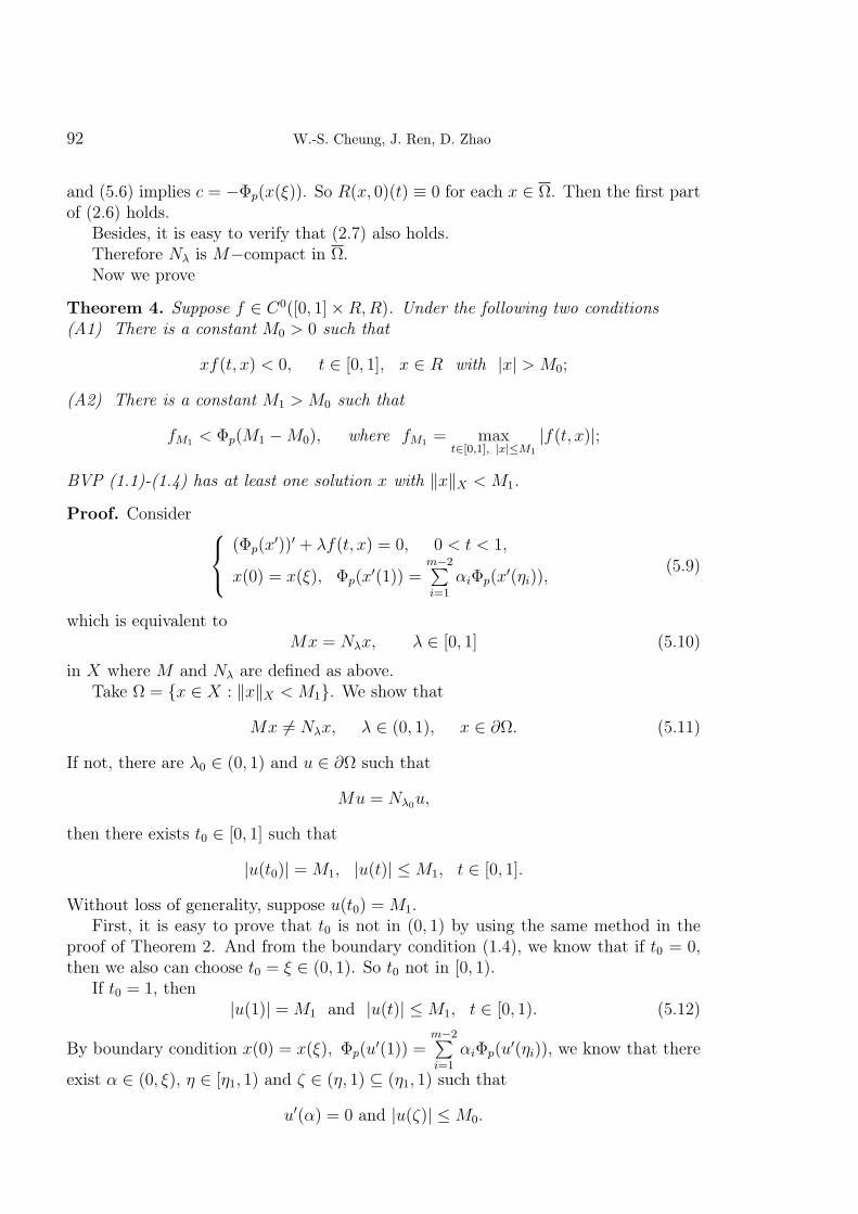
and (5.6) implies c = −Φp(x(ξ)). So R(x, 0)(t) ≡ 0 for each x ∈ Ω. Then the first partof (2.6) holds.

Besides, it is easy to verify that (2.7) also holds.Therefore Nλ is M−compact in Ω.Now we prove


xf(t, x) < 0, t ∈ [0, 1], x ∈ R with |x| > M0;

(A2) There is a constant M1 > M0 such that

fM1 < Φp(M1 −M0), where fM1 = maxt∈[0,1], |x|≤M1

|f(t, x)|;

BVP (1.1)-(1.4) has at least one solution x with ‖x‖X < M1.


′))′ + λf(t, x) = 0, 0 < t < 1,

x(0) = x(ξ), Φp(x′(1)) =

m−2∑i=1

αiΦp(x′(ηi)),

(5.9)



Mx 6= Nλx, λ ∈ (0, 1), x ∈ ∂Ω. (5.11)

If not, there are λ0 ∈ (0, 1) and u ∈ ∂Ω such that

Mu = Nλ0u,

then there exists t0 ∈ [0, 1] such that

|u(t0)| = M1, |u(t)| ≤M1, t ∈ [0, 1].

Without loss of generality, suppose u(t0) = M1.First, it is easy to prove that t0 is not in (0, 1) by using the same method in the

proof of Theorem 2. And from the boundary condition (1.4), we know that if t0 = 0,then we also can choose t0 = ξ ∈ (0, 1). So t0 not in [0, 1).

If t0 = 1, then|u(1)| = M1 and |u(t)| ≤M1, t ∈ [0, 1). (5.12)

By boundary condition x(0) = x(ξ), Φp(u′(1)) =

m−2∑i=1

αiΦp(u′(ηi)), we know that there

exist α ∈ (0, ξ), η ∈ [η1, 1) and ζ ∈ (η, 1) ⊆ (η1, 1) such that

u′(α) = 0 and |u(ζ)| ≤M0.


By Mu = Nλ0u, we have


′(α))−∫ t

α

λ0f(s, u(s))ds, t ∈ [0, 1],

i.e.,Φp(|u′(t)|) = |Φp(u

′(t))| ≤ fM1 , t ∈ [0, 1].

That ismaxt∈[0,1]

|u′(t)| ≤ Φ−1p [fM1 ].

From u(1) = u(ζ) +∫ 1

ζu′(s)ds, we find

M1 = |u(1)| =∣∣∣∣u(ζ) +

∫ 1

ζ

u′(s)ds

∣∣∣∣ ≤ |u(ζ)|+∫ 1

ζ

|u′(s)|ds

≤M0 + maxt∈[0,1]

|u′(t)| ≤M0 + Φ−1p [fM1 ].

SoΦ−1p (fM1) ≥M1 −M0,

i.e.,fM1 ≥ Φp(M1 −M0)

which contradicts assumption (A2).Then (5.10) holds.Similar to the proof of Theorem 3, we also have

degJQN,Ω ∩X1, 0 = degQN, (−M1,M1), 0 6= 0.


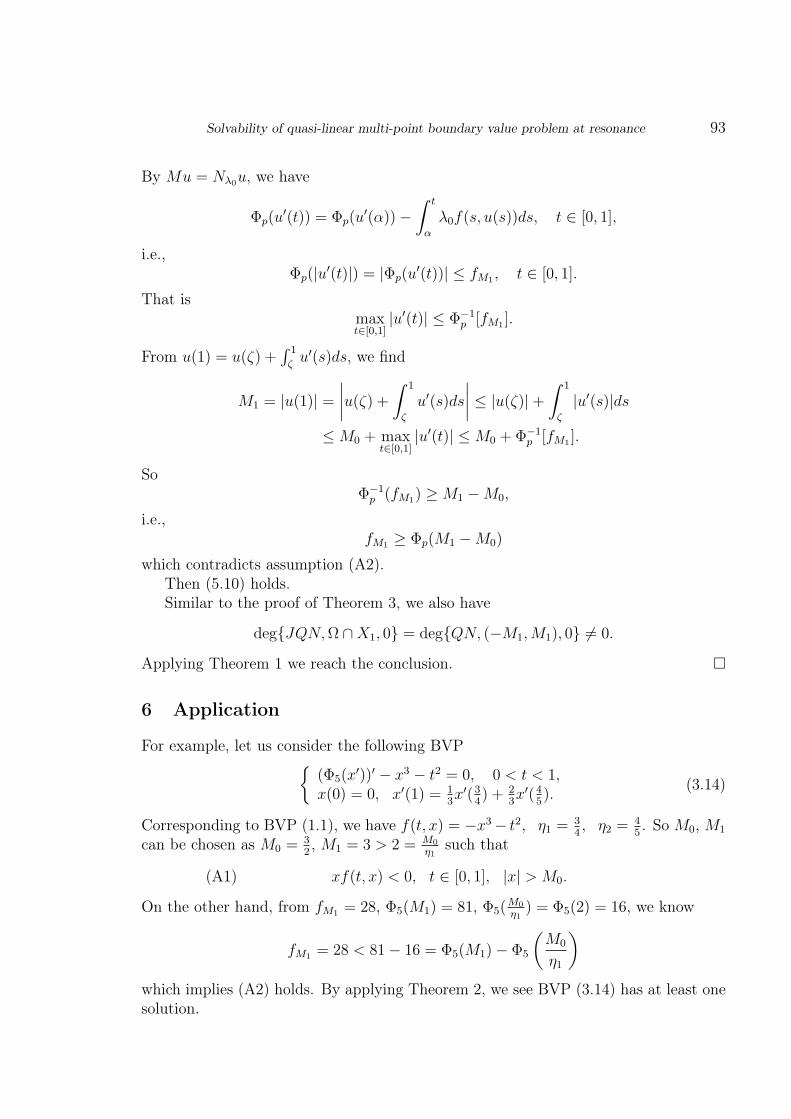
6 Application

For example, let us consider the following BVP(Φ5(x

′))′ − x3 − t2 = 0, 0 < t < 1,x(0) = 0, x′(1) = 1

3x′(3

4) + 2

3x′(4

5).

(3.14)

Corresponding to BVP (1.1), we have f(t, x) = −x3− t2, η1 = 34, η2 = 4

5. So M0, M1

can be chosen as M0 = 32, M1 = 3 > 2 = M0

η1such that

(A1) xf(t, x) < 0, t ∈ [0, 1], |x| > M0.

On the other hand, from fM1 = 28, Φ5(M1) = 81, Φ5(M0

η1) = Φ5(2) = 16, we know

fM1 = 28 < 81− 16 = Φ5(M1)− Φ5

(M0

η1

)which implies (A2) holds. By applying Theorem 2, we see BVP (3.14) has at least onesolution.


References

[1] W.-S. Cheung, J. Ren, On the existence of periodic solutions for a p-Laplacian Rayleigh equation.Nonlinear Analysis TMA, 65 (2006), 2003 – 2012.

[2] W.-S. Cheung, J. Ren, Periodic solutions for p-Laplacian Lienard equation with a deviatingargument. Nonlinear Analysis TMA, 59 (2004), 107 – 120.

[3] W.-S. Cheung, J. Ren, Periodic solutions for p-Laplacian differential equation with multipledeviating arguments. Nonlinear Analysis TMA, 62 (2005), 727 – 742.

[4] W. Feng, J.R.L. Webb, Solvability of three point boundary value problems at resonance. NonlinearAnalysis TMA, 30 (1997), 3227 – 3238.

[5] R.E. Gaines, J.L. Mawhin, Coincidence Degree and Nonlinear Differential Equations. Springer-Verlag, Berlin, 1977.

[6] W. Ge, J. Ren, An extension of Mawhin’s continuation theorem and its application to boundaryvalue problems with a p-Laplacian. Nonlinear Analysis TMA, 58 (2004), 477 – 488.

[7] C.P. Gupta, A second order M -point boundary value problem at resonance. Nonlinear AnalysisTMA, 24 (1995), 1483 – 1489.

[8] G.L. Karakostas, P.Ch. Tsamatos, On a nonlocal boundary value problem at resonance. JMAA,259, no. 1 (2001), 209 – 218.

[9] Bing Liu, Solvability of multi-point boundary value problem at resonance. Applied Mathematicsand Computation, 136 (2003), 353 – 377.

[10] B. Przeradzki, R. Stanczy, Solvability of a multi-point boundary value problem at resonance.JMAA, 264, no. 2 (2001), 253 – 261.

Wing-Sum CheungDepartment of MathematicsThe University of Hong KongPokfulam Road, Hong KongE-mail: [email protected]

Jingli RenDepartment of MathematicsZhengzhou UniversityZhengzhou, Henan 450052, P.R. ChinaE-mail: [email protected]

Dandan ZhaoDepartment of MathematicsThe University of Hong KongPokfulam Road, Hong KongE-mail: [email protected]

Received: 02.07.2010

EURASIAN MATHEMATICAL JOURNAL2010 – Том 1, 4 – Астана: ЕНУ. – 140 с.

Подписано в печать 30.12.10 г. Тираж – 300 экз.

Адрес редакции: 010010, Астана, ул. Мунайтпасова, 7,Евразийский национальный университет имени Л.Н. Гумилева,

учебно-лабораторный корпус, каб. 411Тел.: +7-7172-352028

Дизайн: К. Булан

Отпечатано в типографии ЕНУ имени Л.Н.Гумилева

c© Евразийский национальный университет имени Л.Н. Гумилева

Свидетельство о постановке на учет печатного изданияМинистерства культуры и информации Республики Казахстан

10330 – Ж от 25.09.2009 г.

eurasian mathematical journalrepository.enu.kz/bitstream/handle/123456789/2739... · eurasian...

Documents