eucys - face detection using swarm intelligence final - face... · 22nd european union contest for...

22nd European Union Contest for Young Scientists

Face Detection using Swarm Intelligence

Andreas Lang

Chemnitz, 31 May 2010

Project Advisor:

Dipl.-Inf. Marc RitterChair Media Computer Science

Chemnitz University of Technology

Andreas Lang EUCYS 2010

Table of Contents

1 Introduction......................................................................................................................................................1

1.1 Face Detection..........................................................................................................................................1

1.2 Swarm Intelligence and Particle Swarm Optimisation............................................................................1

2 Fundamentals....................................................................................................................................................2

3 Face Detection by Means of Particle Swarm Optimisation..............................................................................3

3.1 Swarms and Particles...............................................................................................................................4

3.2 Behaviour Patterns...................................................................................................................................4

3.2.1 Opportunism....................................................................................................................................5

3.2.2 Avoidance........................................................................................................................................6

3.2.3 Other Behaviour Patterns................................................................................................................7

3.3 Stop Criterion...........................................................................................................................................7

3.4 Calculation of the Solution......................................................................................................................8

3.5 Example Application................................................................................................................................9

4 Summary and Outlook......................................................................................................................................9

Andreas Lang EUCYS 2010 1

1 Introduction

Groups of starlings can form impressive shapes as they travel northward together in the springtime. This is among a group

of natural phenomena based on swarm behaviour. The research field of artificial intelligence in computer science,

particularly the areas of robotics and image processing, has in recent decades given increasing attention to the underlying

structures. The behaviour of these intelligent swarms has opened new approaches for face detection as well. G. Beni and J.

Wang coined the term “swarm intelligence” to describe this type of group behaviour. In this context, intelligence describes

the ability to solve complex problems.

The objective of this project is to automatically find exactly one face on a photo or video material by means of swarm

intelligence. The process developed for this purpose consists of a combination of various known structures, which are then

adapted to the task of face detection. To illustrate the result, a 3D hat shape is placed on top of the face using an example

application program.

1.1 Face Detection

Face detection involves the detection of the position and size of faces what is necessary for face tracking in videos [Bar09].

Both of these areas are different from the extraction of facial features and face recognition [Bar09]. In addition to automatic

detection and indexing of video material [Man08], face detection is also used by man-machine interfaces, video monitoring

and other applications [ER09].

The greatest problems with which face detection must contend include differing light conditions, “various head positions,

changed facial expressions and partial covering”. These challenges are overcome by many existing methods through the

use of structural information and the disregarding of colour information. These have the disadvantage, however, of “being

susceptible to errors in highly textured or fragmented scenes”. [ER09]

In the case of high resolution, size and colour depth, these methods result in very high computational demands, greatly

limiting real-time face detection in videos with such characteristics [AAM05]. A process with lower computational

demands is necessary to solve this problem. Instead of structural image information, this is accomplished in this project by

applying particle swarm optimisation (PSO) to the colour information of individual images.

1.2 Swarm Intelligence and Particle Swarm Optimisation

The term “swarm intelligence” describes the collective behaviour of what are usually simple individuals in decentralised

systems. The behaviour of individuals allows the entire system to solve complex tasks. With the aid of swarm intelligence,


it is possible to create computer simulations of biological concepts [Thi08].

A swarm that behaves in this way is characterised “by self-organisation, adaptability and robustness”. Self-organisation is

the “unmonitored and decentralised coordination of tasks”. The adaptability is made apparent by the swarm's ability to find

a good solution under various external conditions. Robustness is the “completion of the task in spite of the failure of a

relatively small number of individuals” [Pin07].

Particle swarm optimisation is an application of swarm intelligence in the area of optimisation. During optimisation, one

attempts to find the minimum of a target function [Bar97]. A special characteristic of PSO is that it generally provides good

results, without the computational complexity typically required for finding the optimum solution [Thi08].

2 Fundamentals

This chapter includes an introduction to the programs used and the mathematical definitions of images, videos, colour

spaces and the colour difference image.

Software

The example application, written in the Java programming language, is integrated in the AMOPA framework, which was

developed within the scope of the Professorship of Media Informatics of the Chemnitz University of Technology (TU

Chemnitz) (see Figure 1) for the creation of image and video processing chains. This framework provides the functionality

for the loading, processing and on-screen display of images and videos [Rit09]. The Open Graphics Library (OpenGL) is

used to visualise 3D objects.

Definition of images and video

An image is represented by a two-dimensional matrix M with H rows and B columns. Each element corresponds to one

pixel (pixel muv, where u specifies the row and v specifies the column) and each possible value of muv corresponds to a grey

tone or colour (see Figure 2) [BB05, Man08].

This is described by M=muv ,0uH ; u ,H ∈ℕ0vB ; v , B∈ℕ∀u∈{0, ... , H−1}∀ v∈{0, ... ,B−1} : muv∈W

[Man08],

where W refers to the used colour space. Three colour spaces are described in the following section.

A video is a sequence of images P f , 0≤ f F ; f , F∈N (in most equations, the frame annotation is omitted

for the sake of clarity). A single image of such a sequence of images is also referred to as a frame.


Definition of colour spaces

In the perception-oriented HSV colour space [Bil02], whose colours are defined by hue H, saturation S and grey value V

with H , S ,V ∈[0 ,1] and which can be represented in a cylinder (see Figure 3), the colour difference q1, 2 between

colour 1 and colour 2 is calculated with:

q1,2=Min∣H 1−H 2∣, 1−∣H 1−H 2∣ [Lat07].

The HSV colour space has the advantage that the saturation and grey value channel have no influence on the calculation of

the colour difference. As a result, people's faces can be detected more independently from their origin and their

corresponding colour of the skin as well as and interfering differences in brightness, caused by shadows on the face, have

no negative impact on the result [SB00]. According to [GL08], the skin colour in images in HSV colour space often has a

hue value of H skin∈[0.02 ,0.10 ] and saturation value of S skin∈[0.27 ,0.57] . If the colour of a pixel lies within

these limits, it can be considered to be a skin colour, i.e. it has the optimum quality – otherwise it has the worst possible

quality.

In addition, in the commonly used RGB colour space [Bil02] (see Figure 3), the colour difference is calculated using the

Euclidean distance; in the NCC colour space, which is based on normalized colour channels and is recommended by

[TSFA00] for face detection, the value is calculated according to [SB00].

Colour difference image

The colour difference image is represented as image matrix Q. Its pixels quv with quv∈[0 ,255] , quv∈N are

calculated from the input image. PSO uses the colour difference image as the search space. A low value for a pixel

corresponds to a good quality and thus means that this position of the original image contains skin colour. In nature, this

corresponds to food [Man08]. A high pixel value corresponds to a poorer quality. In the following, positions and regions

with small colour differences are simply referred to as „good“.

3 Face Detection by Means of Particle Swarm Optimisation

This chapter covers the functional principle of the iterative method of PSO, the objective being to approximate the position

and size of the face that is to be detected. The target function to be optimised corresponds to the difference between

calculated and actual size and position of the face being searched for. Consequently, the minimum of the target function

corresponds to the actual size and position. To achieve this goal, the particles should distribute themselves on the face

during the iterations (Section 3.2). Upon completion of the iterations (Section 3.3), the position and size of the face to be


detected is determined from the positions of the particles (Section 3.4). An overwiev can bee seen in the flow chart in

Figure 6.

One desired feature of this process is robustness. When an individual is in a bad region, it uses the swarm's or its own

knowledge of better positions to move in their direction and can thereby contribute to a good solution. PSO can compensate

for partial covering of the face since a large amount of skin colour is located in the “visible” part of the face in a small area.

A particle is an object that moves according to simple behaviour patterns in the search area. An individual particle does not

make any complex decisions on its own, it only follows simple rules that determine its movements. However,

communication with other particles in the swarm does take place. Behaviour patterns and information exchange give the

particle swarm the ability to detect the largest skin-coloured area (e.g. a face) .

3.1 Swarms and Particles

The swarm S={Pi ∣ i∈ℕ ,0≤i∣S∣} is a set of particles Pi with identification number i.

Pi occupies position X i=uv with u , v∈ℕ , 0uB , 0vH in the search area.

At the start of an iteration process with iteration steps t with 0≤tT ; t , T∈N (the annotation of the iteration

step is omitted in some equations for the sake of clarity) and iteration duration T, all particles are randomly distributed on

the colour difference image, where U, V represent equally distributed random variables: [AAM05]

∀ Pi∈S : X i ,0=UV with U ∈[0, B−1] and V ∈[0, H−1]

In subsequent iteration steps, Pi moves according to certain behaviour patterns in the search area. Pi changes its position on

each iteration step by movement vector Vi, t.

V i ,t=uv; u , v∈ℕ and Xi, t = Xi, t-1 + Vi, t

Vi is calculated from multiple behaviour patterns. The relevance of the individual behaviour patterns to face detection can

be determined in an evaluation upon completion of this project. The used behaviour patterns are explained in the following

sections.

3.2 Behaviour Patterns

The behaviour patterns are defined such that the PSO approaches an optimum solution over the course of the iterations.


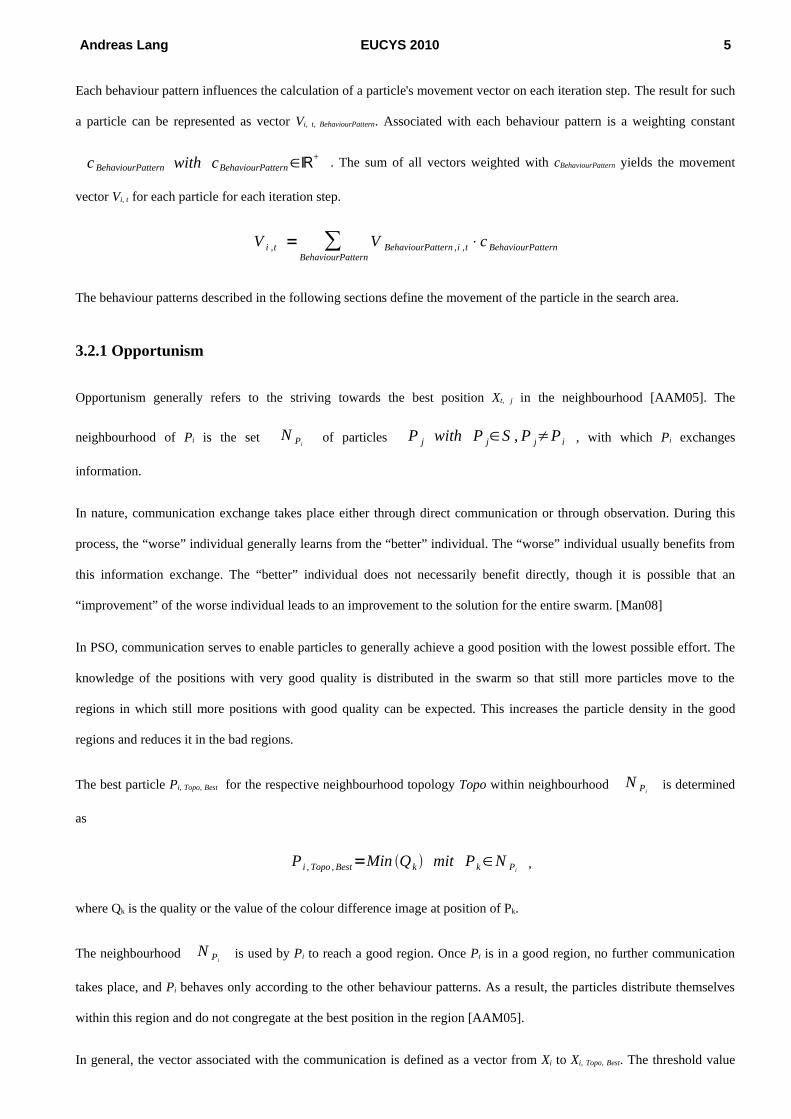
Each behaviour pattern influences the calculation of a particle's movement vector on each iteration step. The result for such

a particle can be represented as vector Vi, t, BehaviourPattern. Associated with each behaviour pattern is a weighting constant

c BehaviourPattern with cBehaviourPattern∈ℝ+ . The sum of all vectors weighted with cBehaviourPattern yields the movement

vector Vi, t for each particle for each iteration step.

V i ,t = ∑BehaviourPattern

V BehaviourPattern ,i ,t⋅c BehaviourPattern

The behaviour patterns described in the following sections define the movement of the particle in the search area.

3.2.1 Opportunism

Opportunism generally refers to the striving towards the best position Xt, j in the neighbourhood [AAM05]. The

neighbourhood of Pi is the set N Pi of particles P j with P j∈S , P j≠Pi , with which Pi exchanges

information.

In nature, communication exchange takes place either through direct communication or through observation. During this

process, the “worse” individual generally learns from the “better” individual. The “worse” individual usually benefits from

this information exchange. The “better” individual does not necessarily benefit directly, though it is possible that an

“improvement” of the worse individual leads to an improvement to the solution for the entire swarm. [Man08]

In PSO, communication serves to enable particles to generally achieve a good position with the lowest possible effort. The

knowledge of the positions with very good quality is distributed in the swarm so that still more particles move to the

regions in which still more positions with good quality can be expected. This increases the particle density in the good

regions and reduces it in the bad regions.

The best particle Pi, Topo, Best for the respective neighbourhood topology Topo within neighbourhood N Pi is determined

as

Pi , Topo , Best=Min Qk mit Pk∈N Pi,

where Qk is the quality or the value of the colour difference image at position of Pk.

The neighbourhood N Pi is used by Pi to reach a good region. Once Pi is in a good region, no further communication

takes place, and Pi behaves only according to the other behaviour patterns. As a result, the particles distribute themselves

within this region and do not congregate at the best position in the region [AAM05].

In general, the vector associated with the communication is defined as a vector from Xi to Xi, Topo, Best. The threshold value


cOpportunismThreshold specifies whether a good position exists. The vector for communication in the respective neighbourhood

topology Topo is calculated with:

V i ,Topo , Best={X i ,Topo , Best−X i

0; if QicOpportunismThreshold

;otherwise

Neighbourhood topologies

N Pi Is determined by a neighbourhood topology. The choice of neighbourhood topology influences the result

considerably [Man08]. First, the search area neighbourhood (see Figure 4) of Pi includes all Pj whose Euclidean distance

to Pi in the search area is less than r [AAM05].

N Pi ,SearchAreaNeighbourhood={P j ∣ ∣X j X i∣r}

Second, the index neighbourhood [Man08] is defined by

N Pi , IndexNeighbourhood={P j ∣ j∈ℕ∧[ 0 ,∣S∣) , Min ∣i− j∣,∣∣S∣i− j∣ ≤ n , j≠n , n≤[∣S∣2]} .

This neighbourhood topology can be explained as particles distributed on a ring, where the adjacent particles to the left and

right belong to the neighbourhood [Man08]. Various values exist for n (see Figure 4):

• n = 0 results in no neighbourhood being present. The particles are autonomous and do not communicate

with one another.

• 0n⌊∣S∣2 ⌋ results in each Pi having ∣N Pi∣=2⋅n neighbours, independent of their position.

• n=⌊∣S∣2 ⌋ results in the entire swarm forming the neighbourhood.

3.2.2 Avoidance

The avoidance behaviour pattern causes Pi to be pushed away from particle Pj, P j∈S , with the smallest Euclidean

distance to Pi. This results in a uniform distribution of the particles in a high-quality region, which in turn necessitates

better coverage of the area and an increase in the size of the search area, since not all particles are seeking out the very best

positions.

V i , Avoidance=X i−X j

∣X i−X j∣,where ∀ k∈ℕ , 0≤k∣S∣ : ∣X j−X i∣≤∣X k−X i∣ [AAM05]


3.2.3 Other Behaviour Patterns

The memory behaviour pattern causes Pi to try to return to the position it previously determined to be the best. To

accomplish this, on each iteration Pi compares the quality of the position it has thus far determined to be the best with the

quality of the current position and, if determined to be better, stores the current position with the corresponding quality

[Man08].

The alignment of the movement vector of a particle with the movement of the entire swarm results in a reduction in the

fluctuation and allows a face to be tracked over multiple frames of a video. Alignment with particles within a

neighbourhood is also conceivable [Rey99].

V i ,t , Alignment=∑Pi∈S

V i ,t−1

∣S∣

The sluggishness controls the influence of new decisions on the movement of a particle by including the previous

movement vector in the current movement [ESK01].

V i ,t , Sluggishness=V i ,t−1

The maximum speed of a particle is limited to vmax [Man08]. If, at the start of the PSO, particles still move large distances

over the entire image in order to find a good region, towards the end, they should only move within this region at lower

speeds. Annealing is realised by means of a gradual reduction in the maximum speed according to the following equation:

∣V i∣=v max ,t , if ∣V i∣v max, t with vmax , t=cVmax⋅cmaxAnnealingt ∧cmaxAnnealing1 .

3.3 Stop Criterion

In order to end the particle-movement process described in the previous section, there is a stop criterion of which two

variants were used simultaneously in this project.

• End the iteration process after a defined number of iteration steps. The advantage of this variant is that one has a

result after a set period of time, which is important for real-time applications [Man08].

• End the iteration process after swarm activity approaches a standstill, i.e. when the activity of the swarm falls

below a set limit value. The advantage of this variant is that one can reduce the used computational resources as

soon as additional iterations no longer yield considerable improvements in the result. The activity can either be

calculated according to [AAM05] as the sum of the contributions of the movement vectors of all particles or

according to [Man08] as the sum of the quality improvements of all particles.


3.4 Calculation of the Solution

To determine the solution in the PSO, normally either the particle of the swarm with the best position is used [Man08] or

the entire swarm is utilised [AAM05]. This project uses a combination of both. Because all particles located on the face

should ultimately contribute to the solution and all others should ideally be excluded, a selection takes place in two phases,

where the second phase simultaneously serves to calculate the solution.

Selection by quality

With selection by quality, individual outliers that are located in a position of poor quality on the last iteration step, i.e. not

on the face, are sorted out. The set SSelectionByQuality with S SelectionByQuality∈S is the result of selection by quality in

which the portion cSelectionByQuality with cSelectionByQuality∈( 0 ,1 ] of the best particles is selected from S .

SSelectionByQuality={Pi ∣ Pi∈S , QiMinimumQuality}with MinimumQuality=ParticlesSortedByQ [⌊∣S∣⋅cSelectionByQuality ⌋]a nd ParticlesSortedByQ=sort {Qi ∣ Pi∈S }

Selection by distance and calculation of position and size

If, during the selection process, only particles with poor quality are detected, selection by distance chooses those that have

good quality but are still far from the main part of the swarm. This is the case, for example, if particles have collected on a

hand that is located in a region other than the face. The number nSelectionDistance of particles included in the calculation of

position and size is calculated using:

nSelectionDistance=⌈cSelectionDistance⋅∣S SelectionQuality∣⌉ with cSelectionDistance ∈ ( 0 ;1 ] .

The set SSelectionDistance of particles selected by distance and the position XS of the face as the centroid of points contained in

SselectionDistance are calculated iteratively. At the start of the iteration SSelectionDistance=S SelectionQuality . In each iteration step,

the position vector of the centroid X S SelectionDistance of particles contained in SselectionDistance is calculated according to

OX SSelectionDistance=

∑Pi∈S SelectionDistance

OX i

∣S SelectionDistance∣.

The particle located the greatest distance from the centroid is deleted from SSelectionDistance. Iteration ends if |SSelectionDistance| =

nSelectionDistance. The size of the face is expressed by the radius. The radius is the distance from XS to the particle in SSelectionDistance

located the greatest distance away at the end of the iteration process.


3.5 Example Application

Using the graphical user interface (GUI), whose class diagram is shown in Figure 5, the user can change default

parameters, start face detection and display the starting image or a video with projected 3D hat. Optionally, the colour

difference image can also be displayed. With image sequences, the particle positions of the last iteration step of the current

frame are used as the starting positions for the particles of the next frame in order to facilitate real-time processing of the

data.

∀ Pi∈S : X i , 0, f 1=X i , T−1, f

Example results of program execution, always using the same parameters, are shown in Figures 7 and 8.

4 Summary and Outlook

The initial image or the first frame of a video is first converted to a colour difference image. PSO is performed on this

image, whereby the particles are randomly distributed over the entire image during the initialisation phase. They then

gradually gather on the face region. After the selection has been made, a 3D hat shape is projected onto the detected face.

For videos, this process is repeated for face tracking in each frame. In this case, the current particle positions are passed on

to the subsequent image.

The evaluation in Table 1 shows that faces can be detected despite of image noise, partial covering or turning of the face. In

a more extensive automatic evaluation performed upon completion of this project and simplified by the integration in

AMOPA, it would be possible to improve the results by evaluating the best parameters for the method using annotated

image databases. Furthermore, the method might also be used within AMOPA as a singular module to accelerate further

image processing operations.

The problem of detecting multiple faces in an image can be solved through the use of clustering techniques which serve to

determine groups of individual objects in a feature space. Following the iteration of the PSO particle groupings for various

faces could be detected. At the same time, smaller groups of particles located over interferings, i.e. smaller areas with

colours similar to that of skin could be specifically ignored.


Appendix

Figure 2: Structure of an image represented by the matrix P. (source: [Man08])


Figure 4: Left: Search area neighbourhood: Belonging to the search area neighbourhood of P1 are those particles (P3

and P4) that are located within radius r around P1. All other particles (P2, P5) are not part of the neighbourhood.

Middle: Index neighbourhood with n=1. Each particle communicates with exactly one particle to its left and one to its

right (e.g. P9 with P8 and P10). Right: “global best”: the entire swarm forms the neighbourhood (Source: [Man08]).

Figure 3: Left: Similar to the HSV colour space, “HLS colour space as a cylinder with the coordinates H (hue)

as angle, S (saturation) as radius and L (lightness) [corresponds to V] as distance along the vertical axis which

runs between black point S and white point W.” Right: “The primary colours red (R), green (G) and blue (B)

form the coordinate axes. The “pure” colours red (R), green (G), blue (B), cyan (C), magenta (M) and yellow

(Y) lie at the corner points of the colour cube. All grey values, such as colour point K, lie on the diagonals

(“uncoloured lines”) between black point S and white point W.” (source: [BB05])


Figure 7: Program execution with various images. Small, orange circles represent the particles. A large, green circle

describes the size and position of a given face. Shown in the images are people of different origin (upper left: Peruvian

woman [Qui06]. Upper right: child from Togo [Zuz09]. Middle left: Polynesian man [Raw07]. Middle right: English man

[Boy08]).


Figure 8: Left: Colour difference table of the image from [Boy08]. Right: Original image from [Boy08] with hat.


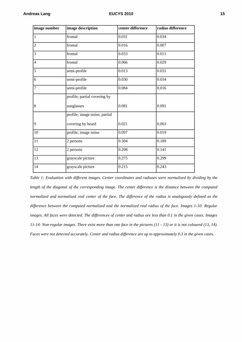
image number image description center difference radius difference

1 frontal 0.031 0.034

2 frontal 0.016 0.007

3 frontal 0.033 0.011

4 frontal 0.066 0.029

5 semi-profile 0.013 0.031



8

profile; partial covering by

sunglasses 0.081 0.091

9

profile; image noise; partial

covering by beard 0.021 0.063

10 profile; image noise 0.097 0.019

11 2 persons 0.304 0.189

12 2 persons 0.208 0.141

13 grayscale picture 0.275 0.299

14 grayscale picture 0.215 0.243

Table 1: Evaluation with different images. Center coordinates and radiuses were normalized by dividing by the

length of the diagonal of the corresponding image. The center difference is the distance between the computed

normalized and normalized real center of the face. The difference of the radius is analogously defined as the

difference between the computed normalized and the normalized real radius of the face. Images 1-10: Regular

images. All faces were detected. The differences of center and radius are less than 0.1 in the given cases. Images

11-14: Non-regular images. There exist more than one face in the pictures (11 - 13) or it is not coloured (13, 14).

Faces were not detected accurately. Center and radius difference are up to approximately 0.3 in the given cases.


Database 1: Database for the Evaluation in Table 1. Images are downloaded from www.flickr.com or self-made.

Copyrights are maintained.

image 1 image 2 image 3 image 4

image 6 image 7

image 9 image 10 image 11 image 12

image 13

image 5 image 8

image 14


Bibliography

[AAM05] Babak Nadjar Araabi, Majid Nili Ahmadabadi, Hossein Mobahi: Swarm Contours: A Fast Self-Organization

Approach for Snake Initialization, 2005.

[Bar09] Kai Uwe Barthel: Facedetection / Gesichtserkennung, 2009. URL

http://www.f4.htw-berlin.de/~barthel/veranstaltungen/WS09/ComputerVision/03_CV_Facedetection.pdf (Online: accessed

22-December-2009)

[Bar97] Hans-Jochen Bartsch: Taschenbuch mathematischer Formeln, Fachbuchverlag Leipzig 1997.

[BB05] Wilhelm Burger und Mark James Burge: Digitale Bildverarbeitung. Eine Einführung mit Java und ImageJ,

Springer-Verlag Berlin Heidelberg 2005.

[Bil02] Ralf Bill: Themenrundgang Farbmodelle, 2002. URL http://www.geoinformatik.uni-

rostock.de/rundgangeinzel.asp?ID=467384774 (Online: accessed 23-October-2009)

[Boy08] David Boyle: DSC08059, 2008. URL http://www.flickr.com/photos/beglen/2365920716/ (Online: accessed 4-

January-2010)

[ER09] Eva Eibenberger, Christian Rieß: Farbbasierte Gesichtsdetektion, 2009. URL

http://www5.informatik.uni-erlangen.de/lectures/ws-0910/farbbasierte-gesichtsdetektion-sem-fg/ (Online: accessed 22-

December-2009)

[ESK01] Russell C. Eberhart, Yuhui Shi und James Kennedy: Swarm Intelligence, Academic Press London 2001.

[GL08] David C. Gibbon, Zhu Liu: Introduction to video search engines, Springer-Verlag Berlin Heidelberg, 2008.

[Lat07] Christian Latsch: Personentracking über adaptive Hintergrund- und Differenzbildberechnung. Studienarbeit im

Studiengang Computervisualistik, 2007. URL http://kola.opus.hbz-nrw.de/volltexte/2008/277/pdf/Studienarbeit.pdf

(Online: accessed 23-October-2009)

[Man08] Robert Manthey: Diplomarbeit. Entwurf und Implementierung eines Verfahrens zur automatischen

Segmentierung von Bild- und Videodaten mittels Partikelschwärmen, Professur Medieninformatik, TU Chemnitz, 2008.

[Pin07] Lydia Pintscher: Schwarmintelligenz, 2007. URL http://www.lydiapintscher.de/uni/schwarmintelligenz.pdf

(Online: accessed 28-December-2009)

[Qui06] Thom Quine: Sun Sombrero, 2006. URL

http://www.flickr.com/photos/quinet/109982470/in/set-72057594049067346/ (Online: accessed 4-January-2010)

[Raw07] Duncan Rawlinson: aus Tahiti Part 2 French Polynesia October 2007, 2007. URL


http://thelastminuteblog.com/photos/album/72157603107650871/photo/1977767960/tahiti-part-2-french-polynesia-october

-2007-.html and www.photographyicon.com (Online: accessed 4-January-2010)

[Rey99] Craig W. Reynolds: Steering Behaviors For Autonomous Characters, 1999. URL

http://www.red3d.com/cwr/steer/gdc99/ (Online: accessed 23-October-2009)

[Rit09] Marc Ritter: Visualisierung von Prozessketten zur Shot Detection. In: Maximilian Eibl, Jens Kürsten, Marc Ritter

(Hrsg.): Workshop Audiovisuelle Medien WAM 2009, Chemnitz, 2009, S. 135 – 150, Professur Medieninformatik, TU

Chemnitz, 2009. URL http://archiv.tu-chemnitz.de/pub/2009/0095/data/wam09_monarch.pdf (Online: accessed 19-

October-2009)

[SB00] Gijs Stijnman, Rein van den Boomgaard: Background Extraction of Colour Image Sequences using a Gaussian

mixture model, 2000.

[Thi08] Stefanie Thiem: Diplom Thesis. Swarm Intelligence Simulation, Optimization and Comparative Analysis, Professur

Modellierung und Simulation, TU Chemnitz, 2008.

[TSFA00] Jean-Christophe Terrillon, Mahdad N. Shirazi, Hideo Fukamachi, Shigeru Akamatsu: Comparative

Performance of Different Skin Chrominance Models and Chrominance Spaces for the Automatic Detection of Human

Faces in Color Images, 2000.

[Zuz09] Andrea Zuzzu: aus Fotostream von Andrea Zuzzu, 3.2.2009. URL

http://www.flickr.com/photos/34678840@N03/3249984819/sizes/l/in/datetaken/ (Online: accessed 4-January-2010)

Acknowledgements

I would like to thank

Marc Ritter, who tirelessly supported me during my work on the project,

Robert Manthey, who was able to answer all of my questions on particle swarmoptimisation and

Stefan Borgwardt, Beate Lang and Jens Lang for proofreading.

eucys - face detection using swarm intelligence final - face... · 22nd european union contest for...

Documents