euclidean distance mapping

COMptrn~R ORAPmcs AND ~.AGE PROCESS~qG 14, 227-248 (1980)

Euclidean Distance Mapping

PER-ERIK DANIELSSON

Department of Electrical Engineering, Linkoping University, Linkoping $-581 83, Sweden

Received June 5, 1979; revised September 28, 1979; accepted February 6, 1980

Based on a two-component descriptor, a distance label for each point, it is shown that Euclidean distance maps can be generated by effective sequential algorithms. The map indicates, for each pixel in the objects (or the background) of the originally binary picture, the shortest distance to the nearest pixel in the background (or the objects). A map with negligible errors can be produced in two picture scans which has to include forward and backward movement for each line. Thus, for expanding/shrinking purposes it may compete very successfully with iterative parallel propagation in the binary picture itself. It is shown that skeletons can be produced by simple procedures and since these are based on Euclidean distances it is assumed that they are superior to skeletons based on d4- , ds- , and even octagonal metrics.

1. INTRODUCTION

Dis tance m a p p i n g is f requent ly used in p ic ture processing. Usual ly , it is b a s e d on one of the metr ics

d 4 ( ( i , j ) , ( h , k ) ) = [ i - - hi + IJ - k l ,

which is cal led the "c i ty b lock d is tance ," or

ds(( i , j ) , ( h , k ) ) = m a x ( I / - h I, [ j - k l ) ,

which is cal led the " c h e s s b o a r d d is tance ," or a c o m b i n a t i o n of these, e.g., the so-cal led oc tagona l dis tance. Obvious ly , we assume tha t i,j, h, k are integers in the two-d imens iona l r ec tangu la r space.

G iven a b ina ry image with two set of pixels,

S = set of l ' s , the objec ts

= set of O's, the b a c k g r o u n d

a distance map L ( S ) is an image such that for each pixel

( i , j ) E S

there is a co r re spond ing pixel in L ( S ) where

L ( i j ) =

i.e., each pixel in S has b e e n ass igned a label in L ( S ) tha t a moun t s to the d i s tance to the neares t b a c k g r o u n d S. Obv ious ly we can def ine a s imi lar m a p L ( S ) for the background .

227 0146-664X/80/11022%22502.00/0 Copyright © 1980 by Academic Press, Inc.

All rights of reproduction in any form reserved.

228 P E R - E R I K D A N I E L S S O N

The computational procedure

L: S---~ L (S )

is called distance mapping. Distance maps can be used for several purposes [1, 3]. Among these are expan-

sion/shrinking of the objects S (by thresholding L(S) /L(S) ) , construction of shortest paths between points, skeletonizing and shape factor computation [6].

Two principally different methods can be used for distance mapping: sequential (recursive) algorithms or parallel algorithms. In sequential algorithms the picture is scanned and L(i , j ) is computed using recently computed values from the present scan in the neighborhood, e.g., L ( i - 1,j) and L ( i , j - 1). The net effect is that distance labels may propagate across the entire picture in one scan. Such algorithms were first presented by Rosenfeld and Pfaltz [2] for the d4-metric.

In parallel algorithms a sequence of distance maps are generated.

S - ~ L , ( S ) = L,---~ L2(L,) = L 2 - ~ . . . - ~ L . ( L . _ , ) = L. = L (S) .

where each computed label Lk(i,j) in the map L k depends on a neighborhood, e.g.,

Lk_,( i , j ) , i , j < l,

in the previous map L k_ l only. Thus, for each iteration from L k_ ! to Lk, labels can only propagate at a distance that equals the size of the neighborhood. This fact makes parallel distance mapping rather slow compared to sequential algorithms unless physically parallel logic is employed for each pixel.

Distance maps based on the metrics d 4 and d a deviate quite substantially from the ideal Euclidean metric

de((i,j),(h,k)) = ~/(j - i) 2 + (k - h) 2 .

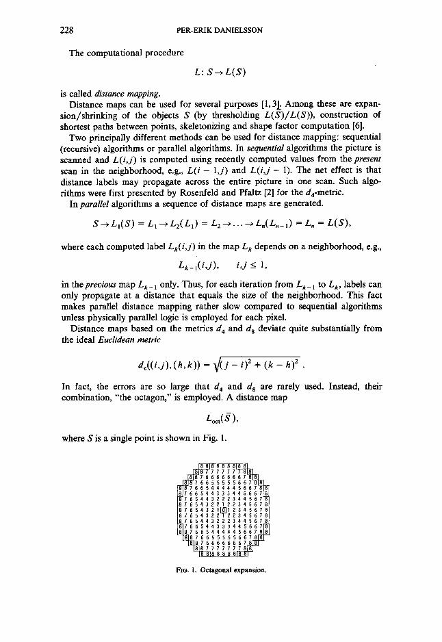
In fact, the errors are so large that d 4 and d 8 are rarely used. Instead, their combination, "the octagon," is employed. A distance map

Lo~,(g),

where S is a single point is shown in Fig. 1.

~ 8 8 ~

6 6 6 7 8 8L8J~ 5 g 66,8 4 45667818 I 3 34456781

(8,65432)~)2345678( 187654321 l [876543 22~2234 5678123456781 ~ 7 6 5 4 4 3 2 2 2 3 4 4 5 6 7 ~ J8176654433344 566718 I 8~876654444456678181

8L81876655555667881.~ I81876666666788~J

EUCLIDEAN DISTANCE MAPPING 229

The best approximation of a circular disc with radius 8 is seen to be somewhat smaller than the object covered by the octagon expanded area up to distance 8. Relative errors above 10% are abundant in octagonal maps and absolute errors far above the pixel units occur for larger distances.

The inaccuracy (even in the octagon case) of distance mapping has recently led a few authors to take an interest in the problem of "circular propagation" of binary images [7-9]. This is essentially equivalent to the problem of Euclidean distance mapping since the goal is to expand the objects a certain Euclidean distance (or the "correct" approximation thereof) in all directions. Correct circular propagation in binary images seem to be extremely time consuming. Probably, a better choice is octagonal propagation interlaced with a "rounding" operation [9, 10]. This method produces a rather good circular approximation for a single point expansion even at larger radii. However, some minor unpredictable results occur when many-point objects are expanded.

Montanari [4] has investigated a type of quasi-Euclidean distance mapping. The distance between two points is defined as the length of the shortest chain-coded path and each step of the path can, in the simplest case (order 1), be selected from the 4 possible steps in the d 4 neighborhood. In this case the distance map is equivalent to a d4-ma p. The quasi-Euclidean map of order 2 selects the steps from the 8 possible cases in the ds-neighborhood. The resulting map is not equivalent to a ds-ma p, however, since each step contributes with its true Euclidean distance. The quasi-Euclidean distance map of order 3 select the steps from a 5 × 5 neighborhood which gives 24 possibilities, etc. It is proved that a shortest path between two points always consists of no more than two different types of steps, namely those having slopes that are closest to the slope of the Euclidean vector between the points. The distance maps can be produced by sequential algorithms in two raster scans. The map of order 2 gives relative errors of 8% in the 22.5 ° directions which makes it comparable in accuracy to octagonal maps. So, to get a improved accuracy one has to use rather large neighborhoods. Even then, the skeletons seem to suffer from the deviations from the exact Euclidean metric.

Barrow et al. [11] uses a distance mapping which is essentially the same as the one of Montanari of order 2 although the relative lengths of the steps V~ : 1 are approximated to 3:2. A sequential algorithm for this case is given in [11].

Algorithms for true Euclidean distance mapping are not to be found in the literature. The advantages of such maps are quite obvious, however, especially if they can be computed efficiently.

2. FOUR-POINT SEQUENTIAL EUCLIDEAN DISTANCE MAPPING

The picture L is a two-dimensional array with the elements

L ( i , j ) 0 < i < M - 1 ,0 < j < N - 1.

Each element is a two-element vector

7-, = ( Li, Lj ), Li, Lj being positive integers,

L(i,j) = ( Li(i,j), Lj(i,j)). The size of a vector L(i,j) is defined by

I L ( i , j ) l = ~ + L2 .

230 PER-ERIK DANIELSSON

The four-point sequential Euclidean distance mapping algorithm 4SED is defined as follows.

4SED

Initially:

£ ( i , j ) ---- (0, 0) if ( i , j ) ~ S,

£ ( i , j ) = ( Z , Z ) if ( i , j ) E S,

where Z is the largest integer that can be stored without inconvenience and where S is the object and S is the background in the original M x N binary picture.

First picture scan: F o r j = 1,2 . . . . . N - 1,

for i = 0, 1,2 . . . . . M - 1,

/~( i , j ) _-- m i n I L - ( i ' j ) [ L ( i , j - 1) + (0, 1);

for i = 1,2 . . . . . M - 1,

mini /~( i , J ) E ( i , j ) [ / ~ ( i - 1,j) + (1,0);

for i = M - 2, M - 3 . . . . . 1,0,

mini E ( i , j ) L ( i , j ) -- [ /~ ( i + 1,j) + ( l ,0) .

Second picture scan: F o r j - - N - 2, N - 3 . . . . . 1,0,

for i --

L ( i , j ) =

for i --

£ ( i , j ) ---

for i =

L ( i , j ) --

0, 1,2 . . . . . M - 1,

rain{ if" ( / ' J) L ( i , j + 1) + (0, 1);

1,2 . . . . . M - 1,

min{ E ( i ' j ) / ~ ( i - l , j ) + (1,0);

M - 2, M - 3 . . . . . 1,0,

mini L ( i , j ) [ /~ ( i + 1,j) + (1,0).

The algorithm first assigns a maximum label to all background pixels. The real assignments take place in two scannings of the complete picture where each picture


74 64 54 44 34 24 14 23 13 03 13 23 33 43 53 63

73 63 53 43 33 23 13 22 12 02 12 22 32 42 52 62

64 62 52 42 32 22 12 02 I I Ol I I 21 31 41 51 Ol

63 52 43 41 31 21 i i 01 10 [ ~ 10 20 30 40 50 60

62 52 42 32 22 20 1(3 [ ~ lO 20 30 40 50 60 70 80

61 51 41 31 21 I I Ol I I 21 31 41 51 61 71 81 91

60 50 40 30 20 10 [ ~ I0 20 30 40 50 60 70 80 90

ZZ ZZ ZZ ZZ ZZ ZZ ZZ ZZ ZZ ZZ ZZ ZZ ZZ ZZ ZZ ZZ

Fio. 2. After first picture s c a n .

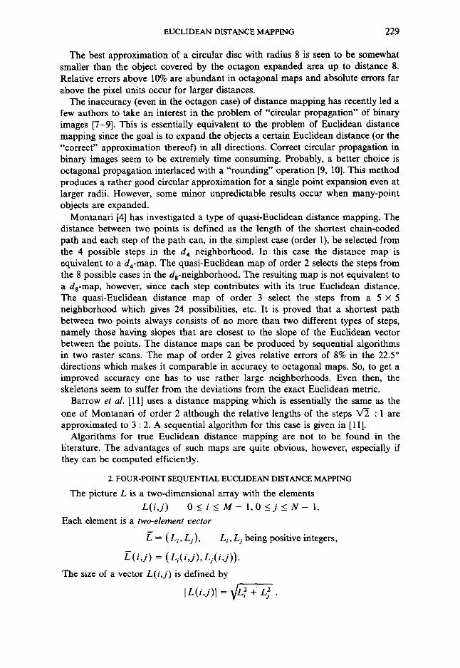
scan involves for each line j first a one-step propagation in the j-direction, then a sequential propagation in both/-directions. In total, each label [( i , j ) is involved in six comparisons.

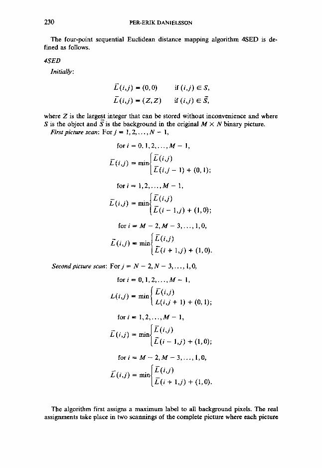
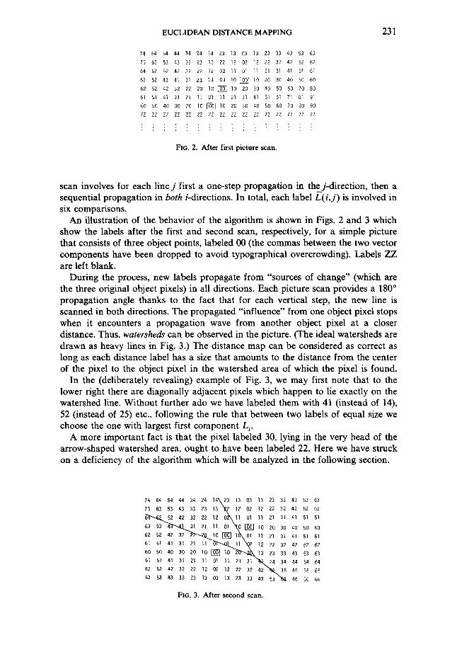
An illustration of the behavior of the algorithm is shown in Figs. 2 and 3 which show the labels after the first and second scan, respectively, for a simple picture that consists of three object points, labeled 00 (the commas between the two vector components have been dropped to avoid typographical overcrowding). Labels ZZ are left blank.

During the process, new labels propagate from "sources of change" (which are the three original object pixels) in all directions. Each picture scan provides a 180 ° propagation angle thanks to the fact that for each vertical step, the new line is scanned in both directions. The propagated "influence" from one object pixel stops when it encounters a propagation wave from another object pixel at a closer distance. Thus, watersheds can be observed in the picture. (The ideal watersheds are drawn as heavy lines in Fig. 3.) The distance map can be considered as correct as long as each distance label has a size that amounts to the distance from the center of the pixel to the object pixel in the watershed area of which the pixel is found.

In the (deliberately revealing) example of Fig. 3, we may first note that to the lower right there are diagonally adjacent pixels which happen to lie exactly on the watershed line. Without further ado we have labeled them with 41 (instead of 14), 52 (instead of 25) etc., following the rule that between two labels of equal size we choose the one with largest first component L r

A more important fact is that the pixel labeled 30, lying in the very head of the arrow-shaped watershed area, ought to have been labeled 22. Here we have struck on a deficiency of the algorithm which will be analyzed in the following section.

74 64 54 44 34 24 14~23 13 03 13 23 33 43 53 63

73 63 53 43 33 23 1 3 ~ 12 02 12 22 32 42 52 62

6 ~ 2 42 32 22 12 O~x l l Ol I I 21 31 41 51 61

63 53 4~'--~..31 zl 11 oi \ o ~ Io 2o 3o 4o so ~o

61 51 41 31 21 I I 0 7 ~ O J ~ l "~g? 12 22 32 42 52 62

60 50 40 30 20 I0 [ ~ I0 2 ~ 1 3 23 33 43 53 63

61 51 41 31 21 I I Ol I I 21 31 ~ 2 4 34 44 54 64

62 52 42 32 22 12 02 12 22 32 42 ~ 35 45 55 65

63 53 43 33 23 13 03 13 23 33 43 53 ~ 46 56 66

FIG. 3. After second scan.


3. ERROR ANALYSIS. THE EIGHT-POINT ALGORITHM

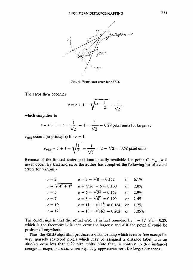
The 4SED-algorithm allows for propagation in all four quadrants but only the four closest neighbors compete in the process of assigning a new label to a given pixel. Since these four neighbors form a nonclosed lattice it is possible that the center pixel ought to be labeled from an object pixel different from any of the object pixels that are nearest to the four neighbors. See Fig. 4.

Here we have three object pixels, X, B and C, for which the (ideal) watersheds are drawn as heavy lines. The question is whether all pixels with center-point in the watershed area of C will be labeled from C. As can be seen, while C is more distant than A and B from the two neighbors to the left and below of P, respectively, P itself, lying in the head of the watershed arrow is closer to C and will not be correctly labeled. Thus, watershed corners in the form of arrowheads constitute an error risk.

It is readily understood that such a risk will be relaxed if the lattice is made more dense, for instance by letting the eight nearest neighbors participate in the propagation processes. Also, since the six neighbors in a hexagonal digitization pattern are more dense then the four adjacent pixels in the Cartesian grid, the errors will be less severe in such a case. On the other hand, since we can never close the box around a pixel completely there is always a (small) chance for the ideal watershed configuration to "sneak into the box and snatch the center pixel."

It is also understood that for the 4SED-algorithm the worst case is the one depicted in Fig. 4 where the watershed arrow penetrates into the box along a 45 ° line. The maximum error in the distance labeling is calculated as follows. The two neighboring pixels to P are at distance r from pixels A and B, respectively. Thus, P will be assigned a label equivalent to a distance r + 1 (the pixel unit distance is set to 1).

The correct distance (from C) is d and the error is

e = r + 1 - d .

Maximum error occurs when d is as small as possible (without causing the watersheds to expand over the two neighbor pixels) which means that C is at distance r + 3 = r from the neighbor pixels. Simple geometry reveals that

r 2 = + - - l ,

v~

r 2 = d 2 - d V ~ + 1 = d - 1 )2 1 +

v2 2'

r=~(d-1) 2 1 + v2 2 '

d = _ _

/

1 ~]._z 1 V~ + V r 2 '

1 r ~ d - - - for larger r, d.

v~


/ /

/

/ s J

• 15 /

FIG. 4. Worst-case error for 4SED.

The error then becomes

which simplifies to

e = r + l - r - - -

e = r + l - 2 V~

1 1

v~ v~ = 0.29 pixel units for larger r.

ema x occurs (in principle) for r ---- 1

emax = 1 + 1 - ~ - - 1 v~ - - -- 2 - X/2 = 0.58 pixel units.

Because of the limited raster positions actually available for point C, era= will never occur. By trial and error the author has complied the following list of actual errors for various r:

r = 2 e - - 3 - V'8 =0 .172 or 6.1%

r -- V ' 4 ~ + 12 e = V ~ - 5 = 0.100 or 2.0%

r = 5 e = 6 - V ~ --0.169 or 2.9%

r = 7 e = 8 - X/-61 = 0 . 1 9 0 or 2.4%

r = l 0 e = l l - ~ = 0 . 1 8 4 or 1.7%

r = 12 e = 1 3 - 1VT62 =0 .262 or 2.05%

The conclusion is that the actual error is in fact bounded by 1 - 1/ V~ = 0.29, which is the theoretical distance error for larger r and d if the point C could be positioned anywhere.

Thus, the 4SED algorithm produces a distance map which is error-free except for very sparsely scattered pixels which may be assigned a distance label with an a b s o l u t e error less than 0.29 pixel units. Note that, in contrast to (for instance) octagonal maps, the r e la t i v e error quickly approaches zero for larger distances.


The eight-point sequential Euclidean distance mapping 8SED is defined as follows.

8SED

Initially:

L( i , j) = (0, 0) for ( i , j) ~ S

L( i , j ) = ( Z , Z ) for ( / , j ) E ff

First picture scan: F o r j -- 1, 2 . . . . . N - 1,

f o r / = 0, 1,2 . . . . . M - 1,

[ /~ ( i , j )

m i n l L ( i - l , j - 1) + (1, 1) E( i , j ) [ L ( i , j - 1) + (0, 1) / [ L ( i + 1,j - 1) + (1, 1);

f o r / = 1,2 . . . . . M - 1,

ff,(i,j) = m i n i / ~ ( i ' j ) [L( ib - l , j ) + (1,0) ;

f o r / = M - 2, M - 3 . . . . . 1,0,

mini L ( i , j ) L ( i , j ) - [ / ~ ( i + l , j ) + (1,0).

Second picture scan: F o r j = N - 2, N - 3 . . . . . I, 0,

f o r i -- 0, 1,2 . . . . . M - 1,

[ L ( i , j )

min~/T(i - 1,j + 1) + (1, 1) 1T(i , j ) | L ( i , j + 1) + (0, 1) / [ L ( i + l , j + I) + (I , 1);

fori = 1,2 . . . . . M - 1,

L- ( i , j ) = min i L- ( i ' j ) [ L ( i - 1, j ) + (1,0);

fori = M - 2, M - 1 . . . . . 1,0,

L( i , j ) -- rain{/-T(i'j)_ L ( i + 1 , j ) + (1,0).


x so A

, ~ t

I

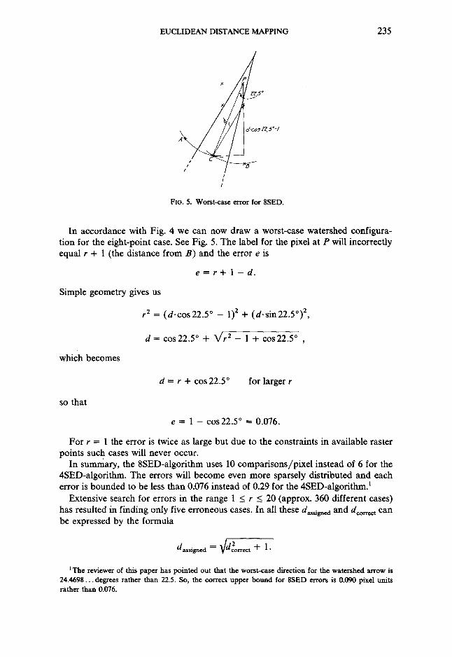
FIO. 5. Worst-case error for 8SED.

In accordance with Fig. 4 we can now draw a worst-case watershed configura- t ion for the eight-point case. See Fig. 5. The label for the pixel at P will incorrect ly

equal r + 1 (the dis tance from B) a n d the error e is

e - - r + l - d .

Simple geometry gives us

r 2 = ( d . c o s 2 2 . 5 ° - 1) ~ + ( d . s i n 2 2 . 5 ° ) 2,

d - - cos22.5 ° + X/r 2 - 1 + cos22.5 ° ,

which becomes

d = r + cos 22.5 ° for larger r

so that

e = 1 - cos22.5 ° -- 0.076.

For r = 1 the error is twice as large bu t due to the constraints in avai lable raster points such cases will never occur.

In summary, the 8SED-algor i thm uses 10 compar i sons /p ixe l ins tead of 6 for the 4SED-algori thm. The errors will become even more sparsely dis t r ibuted a n d each error is b o u n d e d to be less than 0.076 instead of 0.29 for the 4SED-algor i thm. 1

Extensive search for errors in the range 1 < r < 20 (approx. 360 different cases)

has resulted in f inding only five erroneous cases. In all these dassigne d a nd dcorree t c a n be expressed by the formula

2 dassigned ~ ~/deorrect -[- 1.

t The reviewer of this paper has pointed out that the worst-case direction for the watershed arrow is 24.4698... degrees rather than 22.5. So, the correct upper bound for 8SED errors is 0.090 pixel units rather than 0.076.


The largest error in this set of five was for

dassign~ I = 3X/~ = ~132 + 132 ,

dcorrec t = ~ = I V Y + 92

resulting in an absolute error of

1 e = - -

2v33g

and a relative error of

1 .~ 0.027 pixel units

26V~

e ---- 0.15%,

which is negligible for all practical purposes.

4. EUCLIDEAN DISKS AND SKELETONS

Using the notation of [1], a disk Dt(i,j) is the set of all pixels that are at distance < t from (i,j). In what follows we will make a minor change in this definition and define

Dt(i , j) = {(i + h, j + k) fh 2 + k 2 < t2},

i.e., we do not include the pixels that are exactly at distance t. Let us now use the vectorial distance label notation used previously so that

Dab = Dca~+Ki -~ Dba.

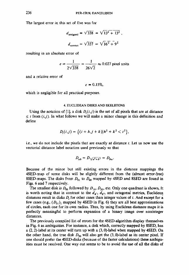
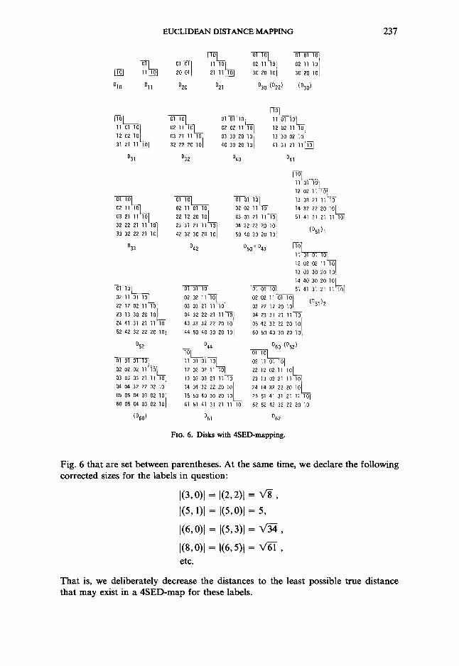
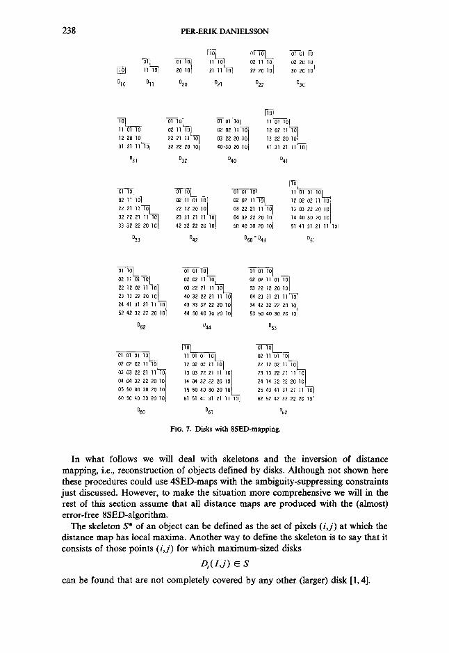
Because of the minor but still existing errors in the distance mappings the 4SED-map of some disks will be slightly different from the (almost error-free) 8SED-maps. The disks from Dol to Dro mapped by 4SED and 8SED are found in Figs. 6 and 7 respectively.

The smallest disk is DOl followed by D n, D2o, etc. Only one quadrant is shown, It is worth noting that in contrast to the d4-, ds-, and octagonal metrics, Euclidean distances result in disks D, for other cases than integer values of t. And except for a few cases (e.g., (D51)1 mapped by 4SED in Fig. 6) they are all best approximations of circles, each one for its own radius. Thus, by using Euclidean distance maps it is perfectly meaningful to perform expansion of a binary image over noninteger distances.

The previously compiled list of errors for the 4SED-algorithm display themselves in Fig. 6 as ambiguities. For instance, a disk which, correctly mapped by 8SED, has a (2, 2)-label at its center will turn up with a (3, 0)-label when mapped by 4SED. On the other hand, the true disk/)3o will also get the (3, 0)-label as its center pixel. If one should prefer the 4SED-disks (because of the faster calculations) these ambiguities must be resolved. One way out seems to be to avoid the use of all the disks of


oI 1 Ir o-q__ o ~ 11 lOL_ 02 02 11 Io I

[ ] I1101 20 011 21 1 1 ~ 30 20 101 30 20 101

DIO Dll D20 D21 030 (D22) (D30)

02 11 02 02 11 1100 12 02 11 i ; 033020 10 1 3 3 0 0 2 1 0 L ~ 12 02 I01_ ~ 03 21 II

31 21 11 101 32 22 20 40 30 20 41 31 21 11101

D31 D32 D40

Ol 10-[~. 01 1 0 1 _ _ 01 O1 I O L 02 11 1 0 ~ 02 11 01 1 0 | 02 02 11

o3 21 11 l o 1 ~ 22 12 2o l o L _ o3 o3 21 11 lo I 32 22 21 II I01 23 31 21 11 10 04 32 22 20 10 33 32 22 21 lO I 42 32 30 20 0 50 40 30 20 lO

D33 042 %0 ~ D43

01 1C) I ~ 01 01 1 0 [ _ _

L _ - 02 11 O1 10 02 02 11 101 02 02 11 01 10 2 2 , 2 o 2 . 10 03 03 21 11 03 22 12 20 10 23 13 30 z0 10 04 32 22 21 11 101 04 23 31 21 11 10 I 24 41 31 21 11 10 43 33 32 22 20 10 05 42 32 22 20 10 52 42 32 22 20 I0 44 50 40 30 20 I0 60 50 40 30 20 I0

D52 D44 D60 (D53} 1 o - i _ _ oi ,o i

02 02 02 11" I0~ 12 02 02 II I 0 ~ 22 12 02 l l l O ~ 23 13 03 21 11 lO 03 03 03 21 11 10 13 03 03 21 11 10 / L_

04 04 32 22 02 10 14 04 32 22 20 I0 24 14 32 22 20 10 05 05 04 03 02 I0 15 50 40 30 20 1 0 [ ~ 25 51 41 31 21 11 I0 60 05 04 03 02 10 61 51 41 31 21 11 I01 62 52 42 32 22 20 I0

(%0) 061 D62

D41

11 O1 10 I 12 02 11 1 0 ~ _

13 03 21 11 lo L

L 14 32 22 20 10 51 41 31 21 l l l0 I

(osl)l

11 O1 O1 lO I 12 02 02 11 1 0 [

L 13 03 30 20 10

14 40 30 20 10

51 41 3/ 21 11

(Ds1) 2

FIG. 6. Disks with 4SED-mapping.

Fig. 6 that are set between parentheses. At the same time, we declare the following corrected sizes for the labels in question:

1(3, 0)l = 1(2, 2)1 = V 8 ,

1(5, 1)1 : 1(5,0)1 = 5,

1(6, 0)l = 1(5, 3)1 = x / ~ ,

1(8, 0)1 = 1(6, 5)1 =- V-61-, etc.

That is, we deliberately decrease the distances to the least possible true distance that may exist in a 4SED-map for these labels.

238

[] % DIO D11

PER-ERIK DANIELSSON

Ol 10 ILl~ 0 011100 0211 20 2111 I0[ 22 20 101

D20 D21 D22

°~°111° ° 02 20 10 30 20

D3 0

Ol 10~_ 01 Ol I01 II Ol IO~ I, 01,0| 02 ,I 10L_ 02 02 11~ 12 021 12 20 10L_ 22 21 11 10 o3 22 20101 13 zz 20 10t__ 31 21 11 IoI az zz zo 10 40.30 20 101 41 31 21 11 lol

D31 D32 D40 D41

Ol I0~_ Ol 10] 02 II IOLI 02 11 Ol I0|

I I,,oL 22122010

33 32 22 20 42 32 22 20 IO

D33 D42

oi

02 02 II I0~ 03 22 21 I 110 I 04 32 22 2010 I 50 40 30 20 101

%0 z D43

IlOL~ 1101 Ol lOL~ 12 02 02 II I01 13 03 22 20101 14 40 30 20 I0~_ 51 41 31.21 II I01

DSI

Ol I0] Ol 01 Iol.. ~ Ol Ol TO] ,oL 02 1101 I01 02 02 II 02 02 1101

22 12 02 l l q ~ 03 22 21 11 10 1 oa 22 12 20 10 23 la 22 20 101 40 32 22 21 11 101j 04 2a 31 21 1110 I 24 41 31 21 l l l - ~ 43 33 32 22 20 10 34 42 32 22 20 52 42 32 22 20 10[ 44 50 40 30 20 lO 53 50 40 30 20 lOJ

D52 D44 D53

~[ Ol 10]__ o,o,o, oL .o,o 02 02 02 11 lOL. - 12 02 02 II 22 12 02 ]I 03 03 22 21 11 I01 13 03 22 21 II l O | 23 13 22 21 11 lO 04 04 32 22 20 lOj 14 04 32 22 20 I O L 24 14 32 22 20 I0 05 50 40 30 20 I0 15 50 40 30 20 I0 25 43 41 31 21 l l l ~ 60 50 40 30 20 lO~ 61 51 41 31 21 11 lOJ 62 52 42 32 22 20 I01

D60 D61 D62

Flo. 7. Disks with 8SED-mapping.

In what follows we will deal with skeletons and the inversion of distance mapping, i.e., reconstruction of objects defined by disks. Although not shown here these procedures could use 4SED-maps with the ambiguity-suppressing constraints just discussed. However, to make the situation more comprehensive we will in the rest of this section assume that all distance maps are produced with the (almost) error-free 8SED-algorithm.

The skeleton S* of an object can be defined as the set of pixels (i,j) at which the distance map has local maxima. Another way to define the skeleton is to say that it consists of those points (i,j) for which maximum-sized disks

D t ( 1 , j ) ~ S

can be found that are not completely covered by any other (larger) disk [1, 4].


This skeleton is nonredundant in the weaker sense that it includes no disk that is completely covered by another single disk. Note, however, that the skeleton is redundant in the stronger sense that a union of two or more disks may cover another disk.

With the help of the disk shapes in Fig. 7, the 8SED-mapped object of Fig. 8 can now be skeletonized, first by intuitive trial-and-error. We start with the largest I L(i,j)] which in this case is 05. Evidently, the three

Dso~ S

and since there are no larger disks these three pixels belong to S*. From Fig. 7 we can infer that a/)50 disk has the label 50 in the center and following neighbors:

320432 405040 320432

Now, there are two 40-1abels along the diagonals in the vicinity of the leftmost 50-1abel and since

4 2 + 0 2 v~ 3 2 + 2 2

these labels indicate that they are centers of D4o'S which are not covered by the closest/)50 and consequently these pixels belong to S*. Then, around the center of a D4o we expect to find the neighbors

22 03 22 30 40 30 22 03 22

But the two ringed 40's have one 30-1abel each along the diagonals which then also belong to the skeleton, etc.

We can now imagine how the total skeleton S* can be locally detected by a local 3 × 3-operator in one picture scan. The skeleton algorithm consists of the following skeleton operator SKED for Euclidean distance maps.

"7 10 O1 O1 01 O1 O1 O1 O1 O1 O1 O1 01 011

lO ~o o~ o~ o~ o~ o~ o~ o~ o~ @ ~ ) ~ ° i l o~ o~ o~ o~ o ~ @ ® ® ® I0 20 @ ~ ~ IO

I0 20 30 04 04 04 21 II Ol Io 2o ~o 4o ( ~ ) 6 ~ ( ~ ~ 4o 3o 2o I o i - 10 20 30 @ 0"~" 0"~" 0 ~ ' @ ~ ' ~ 21 11 1 ' ~ ~o ~o@o~ o~ o~ o~ o ~ ® @ ~ o ~oI lo ~o oz o2 o2 oz oz oz oz oz ( ~ ) l o ( lo ol ol o~ ol ol o~ ol ol ol ol loj

FIG. 8. A Euclidean skeleton.


SKED

If and only if for all h, k _< 1, i.e., for all eight neighbors

IL( i , j ) l ~ Igi_h.j_k( f , ( i + h , j + k))l

then ff,(i,j) is a local maximum and (i , j) ~ S*. The function g i -h j - k is a mapping that translates the label L(i + h , j + k) into the label L,(i,j), should i , j belong to a disk centered at i + h , j + h. The functions g i -h j - k are of two types only, gs for the diagonal neighbors and g4 for the four nearest neighbors.

From the previously discussed D4o and/)so disks we can see that, e.g.,

gs(50) = 32, g,(50) = 40,

g8(40) = 22, g4(40) -- 30.

With reasonably short labels gs and g4 can be stored in a look-up table. Further- more, instead of computing absolute distances from the labels we could simply compare the label L( i , j ) directly (twice, with the two components shifted) with the output from the g8- and g4-tables.

The skeleton S*, being the set of centers for disks that exactly cover S, is a compact description of the binary object (or objects) S. As has been demonstrated

S* ffi SKED(SED(S))

The inverse of this operation, that is to generate SED(S) from S*, will be called SKED-1 and is defined as follows, using a propagation scheme identical to the 8SED-algorithm.

SKED -1

Initialize:

00 if ( i , j ) 6Z S* L ( i , j ) = SED(S) for ( i , j ) E S*.

First scan:

L ( i , j )

L ( i , j ) = max. g , ( L ( i , j + 1))

1 j + 1))

gs(/~(i + l,j + 1)),

maxl /~( i , j ) = +


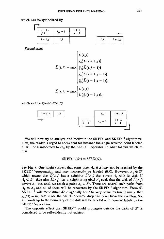
which can be symbolized by

V i - - l , j + l i , j + l

i - 1,j i,j

i + 1 , j + l

Second scan:

J

L(i,j)

~4(E(i + 1,j))

L(i, j) = max o~4(/S(i,j - 1))

~s(/S(i + l , j - 1)) § s ( L - ( i - 1 , j - 1)),

/_~(i,j) = max I E(i,j)

L/~(o~4(i- 1,j)),

which can be symbolized by

I , , . I / . I i,j i + 1,j

i - l , i+1 , j - 1 i , j - 1 j - 1

J

We will now try to analyze and motivate the SKED- and SKED-l-algorithms. First, the reader is urged to check that for instance the single skeleton point labeled 51 will be transformed to Dsi by the SKED -1 operator. In what follows we claim that

S K E D - l ( s * ) = 8SED(S).

See Fig. 9. One might suspect that some pixel A o E S may not be reached by the SKED-l-propagatio_n and may incorrectly be labeled (0, 0). However, A o ~ S* which means that L(Ao) has a neighbor L(Al) that covers A o with its disk. If A I ~ S*, then also L(A 0 has a neighboring pixel A 2 such that the disk of L(A2) covers A~, etc. until we reach a point A 5 E S*. There are several such paths from A o to A 5 and all of them will be recovered by the SKED-l-algorithm. From 53 SKED -I will reconstruct 42 diagonally for the very same reason (namely that ~a(53) = 42) that made the SKED-operator drop this pixel from the skeleton. So, all points up to the boundary of the disk will be labeled with nonzero labels by the SKED- l-algorithm.

The opposite effect that SKED-1 could propagate outside the disks of S* is considered to be self-evidently not existent.

242 PER-ER1K DANIELSSON

I lO 01 01

j lO 01 11 01 02

I0 20 12 22 03

]I0~11-21-31 23 04 A 0

10 20~22~32-"42 34 XAI~Az~A3~A 4 /10 20~'30~,40~50~'53 XA 5

FIo. 9. Paths recovered by SKED-i in reverse direction.

Let us summarize the discussion so far. The skeleton S* = SKED(8SED(S)) defines a number of overlapping Euclidean disks and by applying the S K E D - i . algorithm we can reconstruct 8SED(S) without errors.

What remains to be discussed is whether S* is redundant in the weaker sense that the disk of one skeleton point may completely cover the disk of another.

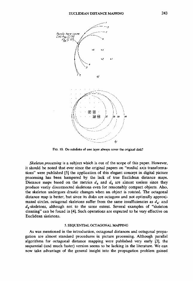
If this could occur we would find the same extra skeleton point by applying the SKED-operator to 8SED(S) where S is a Euclidean disk. As an example of a situation where such a false skeleton point may possibly occur consider the D44-disk of Fig. 7. Evidently, the 8 pixels nearest to the center never run the risk of ending up in S* since they are directly checked in the g4(44) and gs(44) look-up tables. Now, the 8SED-algorithm has produced 32-1abels in the next layer. What guarantee do we have that this label is not of greater size than either g4(33) or g8(50)?

To answer that we have to move to the continuous space again. See Fig. 10, where in Fig. 10a we see the worst case depicted without considering the fact that only a few discrete points are available as pixel centers. The geometry proves to be identical to the previous error analysis picture in Fig. 5. The center pixel 1 has a disk with a certain radius. Its nearest neighbors 2 and 3 are centers of somewhat smaller disks D 2 and D 3 that are completely covered by D~ and are touching D 1 at the horizontal line-crossing and the 45°-line-crossing, respectively. The disk D 4 of point 4, finally, must not contain any point outside the union of D 2 and D 3 which forces D 4 to pass the crossing of D 2 and D 3 in the 22.5°-direction.

Now, assume that D~ includes a pixel in the tiny area outside the union of D 3 and D 2. SKED-1 will reconstruct first D 2 and D 3 and then D 4. But the distance mapping 8SED applied to the binary object D l will produce a label L(4) corre- sponding to the distance between point 4 to a point in this "tiny area". Hence

/~4 v~ g4(E(3))

and

L4 =%= ga(L(2))

and consequently, the SKED-operator will include point 4 in the skeleton S*. Because of the raster points available, this kind of error will be extremely rare. In

fact, not one single case has yet been found. Figure 10b is an illustrative case that motivates our optimism. We see that after

disk D44 follows /)50 which boldly (and correctly) extends beyond D o . And the critical disk/)32 is in fact absolutely as large as possible without covering pixels outside D**.

EUCLIDEAN DISTANCE MAPPING

/

Po/n/s here co, 5e / ~ ~ zJ

x4 x.~

~ 4 ~Z xl

o}

243

FIO. 10. Do subdisks of one layer always cover the original disk?

Skeleton processing is a subject which is out of the scope of this paper. However, it should be noted that ever since the original papers on "medial axis transforma- tions" were published [5] the application of this elegant concept in digital picture processing has been hampered by the lack of true Euclidean distance maps. Distance maps based on the metrics d 4 and d 8 are almost useless since they produce vastly disconnected skeletons even for reasonably compact objects. Also, the skeleton undergoes drastic changes when an object is rotated. The octagonal distance map is better, but since its disks are octagons and not optimally approximated circles, octagonal skeletons suffer from the same insufficiencies as d 4- and ds-skeletons, although not to the same extent. Several examples of "skeleton cleaning" can be found in [4]. Such operations are expected to be very effective on Euclidean skeletons.

5. SEQUENTIAL OCTAGONAL MAPPING

As was mentioned in the introduction, octagonal distances and octagonal propagation are almost standard procedures in picture processing. Although parallel algorithms for octagonal distance mapping were published very early [3], the sequential (and much faster) version seems to be lacking in the literature. We can now take advantage of the general insight into the propagation problem gained


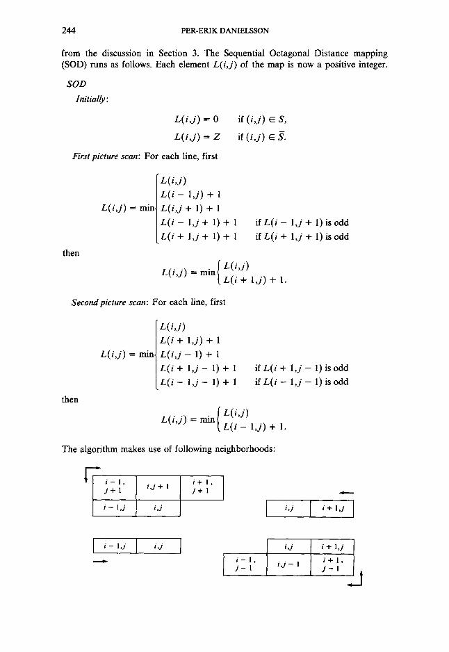
from the discussion in Section 3. The Sequential Octagonal Distance mapping (SOD) runs as follows. Each element L( i , j ) of the map is now a positive integer.

SOD

Initially:

L( i , j ) = 0

L ( i , j ) -- Z

each line, first

"L( i , j )

L ( i - 1,j) + 1

L ( i , j + 1) + 1

L ( i - 1 , j + 1)+ 1

L ( i + 1 , j + 1)+ 1

then

if L( i - 1,j + 1) is odd

if L (i + 1 , j + 1) is odd

First picture scan: For

L ( i , j ) = min,

then

if ( i , j ) E S,

if ( i , j ) ~ S.

rnJn ( L( i , j ) L ( i , j ) = t L ( i + l , j ) + 1.

Second picture scan: For each line, first

L ( i , j )

L ( i + 1,j) + 1

L ( i , j - 1) + 1

L( i + 1 , j - 1)+ 1

L ( i - 1 , j - 1)+ 1

if L( i + l , j - 1) is odd

if L (i - 1 , j - 1) is odd

L ( i , j ) = min

rnin [ L ( i , j ) L ( i , j ) = ( L ( i - 1 , j ) + 1.

The algorithm makes use of following neighborhoods:

I t

i - 1 , i + l , j + i i , j+ 1 j + 1

i - 1,j i , j i ,j ] i + l ,j

i_l , j I i,j I j - I

i , j i + 1,j

i + 1 , i , j - - 1 j - - I


The distance errors in octagonal maps are on the order of 10%. Very often this can be tolerated and if so the octagonal mapping seems to be a good choice since the labels L(i,j) are shorter and the comparisons are much simpler than in the Euclidean case. Note, however, that a total of 10 comparisons has to be done while the 4SED-algorithm required only 6, thanks to the smaller neighborhood depen- dence in the recursion.

Skeletons based on the octagonal distance function can be expected to give many more spurious points and artifacts than skeletons derived from Euclidean distances for two reasons. Firstly, octagonal skeletons represent a set of overlapping octagons instead of circular disks. The octagon shape can be considered much more artificial and rare than a circular boundary. Hence, an original object S is rather cumbersome to match with overlapping octagons. Secondly, Euclidean disks are available for all radii between and including the integer pixel unit distances while octagons only come in unit step sizes.

6. PARALLEL EUCLIDEAN DISTANCE MAPPING

As was said in the introduction, the sequential few-scan algorithms are vastly superior to parallel procedures unless physically parallel hardware exists. Today such true parallel hardware seems rather remote. Still it could be of some interest to see what could be performed in case a Parallel Euclidean Distance Mapping (a PED-algorithm) should be implemented on such a machine. Thus, we assume the existence of a cellular network where each cell corresponds to one pixel (i,j) and has, perhaps rudimentary but still general, logic and arithmetic capability. The basic operation in the distance mapping algorithms is to compare the present label L(i,j) to a neighbor, say/~(i - 1,j), and assign the next label at (i,j)

mini E ( i'j ) L(i,j) = ~ E ( i - 1,j) + (1,0).

The efficiency of the algorithms is most conveniently measured as the total number of comparison steps (executed in parallel at each cell) to perform a certain task. One comparison propagates the labeling one step in one direction and we can call the above operation

P E D / i +

since it propagates labels one step in the positive/-direction. It is readily seen that the sequence

P E D / i + , P E D / i - , P E D / j + , P E D / j -

produces propagation of all labels in the array one step in each direction up to a chessboard distance of 1. That is, each label has the chance to influence its eight neighbors (not only its four nearest neighbors). The relative order of the operations is insignificant.

If the above sequence is iterated t times it is seen that the labeling has propagated so that all pixels up to a distance of t have been labeled and we conclude that to produce a 4SED-map over the chessboard distance t requires 4t comparison steps. The more accurate 8SED-map employs diagonally oriented comparisons so that 8t comparisons are required.


Like many other cases of propagation through a network it is, at least in principle, possible to reduce this to

21og[t + I]

where Ix ] means a power of 2, I x ] / 2 < x < [x]. To achieve this, we have to use connections (which hopefully exist in our parallel machine) so that one label at (i + n,j) can be transferred to the logic cell at (i , j) and execute PED/ni +

L ( i , j ) = min~ I t ( i , j ) l [Z(i - n , j ) + (n,0)] L

and also PED/ni -

L ( i , j ) ----- rain{ ]L(i,j)l

IL(i + n , j ) - (n,0)[.

The operations PED/nj + and PED/nj - are defined in the same manner. We call this operation multistep PED-mapping and the idea is to employ a sequence of these with step sizes which are falling powers of 2:

P E D / n

P E D / n / 2

P E D / 2

PED/1

The principal effect is shown in Fig. 1 l, which shows the steps PED/2 i , P E D / 2 j , PED/1i , P E D / l j .

Q

(-3,t)

\ /

/ \

FIO. 11. Multistep labeling represented by vectors.


Unlike the previous continuous propagation from the objects outwards, label vectors are now planted like seeds in the first two operations. From here, new labels are induced to the adjacent pixels. It may now happen that a final correct label is attained only if a longer vector is allowed to induce a shorter one. Thus, the vector ( - 3 , 2 ) in Fig. l l c induces the vector ( - 3 , 1) in Fig. l l d and this assign- ment requires a signed vector addition.

7. CONCLUSIONS

The most important result of this paper is that Euclidean distances can be produced efficiently by sequential algorithms. The rather simple key is to use a two-component label which makes it possible to propagate in the usual main directions and still keep track of all distances encountered. Distance maps are an alternative to pure binary propagation expansion/shrinking in binary pictures. The cost is of course that one has to use a many-valued ( = nonbinary) image memory, but this disadvantage is rapidly disappearing because of new extremely powerful memory components. A distance map is produced with the 4SED algorithm in two-picture double line-scans regardless of expansion distances and gives a much greater versatility than the pure binary image. The expansion/shrinking distance t achieved after thresholding the map is correctly Euclidean except for a few enumerable cases. Errors in the 8SED map are virtually nonexistent. Somewhat amazingly one can obtain an expanded binary picture for other than integer values of t.

Skeletons are a simple byproduct of distance mapping. Although not treated extensively in this paper, Euclidean skeletons can possibly revive interest in this method for image coding and processing.

In many cases, the octagonal distances are sufficiently accurate and it is possible to produce an octagonal distance map in the same manner as a Euclidean map, namely with sequential propagation in two picture scans. Octagonal distance mapping requires less arithmetic capability and shorter labels.

The parallel algorithms are only interesting if truly parallel hardware is available. In the absence of such hardware they are merely a curiosity.

ACKNOWLEDGMENTS

The author is grateful to Mr. Peter Lord for the final error-checking of the 4SED- and 8SED-algorithms. Also, the anonymous reviewer has had quite an influence on the final version of the paper. His in-depth penetration of the content supports his statement that the algorithms in this paper "are essentially identical to those I have been using since Spring 1977, but have not yet published."

REFERENCES 1. A. Rosenfeld and A. C. Kak, Digital Picture Processing, Academic Press, New York, 1976. 2. A. Rosenfeld and J. Pfaltz, Sequential operations in digital picture processing, J. Assoc. Comput.

Mach. 13, 1966, 471-494. 3. A. Rosenfeld and J. Pfaltz, Distance functions on digital pictures, Pattern Recognition 1, 1968,

33-61. 4. U. Montanari, A method for obtaining skeletons using a quasi-Euclidean distance, J. Assoc.

Comput. Mach. 15, 1968, 600-624. 5. H. Blum, A transformation for extracting new descriptors of shape, in Models for the Perception of

Speech and Visual Form (W. Wathen-Dunn, Ed.), pp. 362-380, MIT Press, Cambridge, Mass., 1967. 6. P. E. Danielsson, A new shape factor, Computer Graphics Image Processing 7, 1978, 292-299.


7. Z. Kulpa, On the properties of discrete circles, rings, and discs, Computer Graphics Image Processing 10, 1979, 348-365.

8. M. Doros, Algorithms for generation of discrete circles, rings, and discs, Computer Graphics Image Processing 10, 1979, 366-371.

9. Z. Kulpa and B. Kruse, Methods of effective implementation of circular propagation in discrete images, Internal Report LiTH-ISY-I-0274, Dept. of Electrical Engineering, Link6ping Univ., Sweden, 1979.

10. B. Kruse, "PICAPO, Description and User's Manual," Internal Report LiTH-Isy-I-0171, Dept. of Electrical Engineering, Link~ping Univ., Sweden, 1977.

11. H. G. Barrow, J. M. Tenenbaum, R. C. Bolles, and H. C. Wolf, Parametric correspondence and chamfer matching: Two new techniques for image matching, Proc., 5th International Joint Con- ference on Artificial Intelligence, 1977, pp. 659-663.

euclidean distance mapping

Documents