ethnic enclaves and the economic success of immigrants
TRANSCRIPT

Ethnic Enclaves and the Economic Success of Immigrants – Evidence from a Natural Experiment*
by
Per-Anders Edin, Peter Fredriksson, and Olof Åslund**
December 14, 2000
Abstract Recent immigrants tend to locate in ethnic ”enclaves” within metropolitan areas. The economic consequence of living in such enclaves is still an unresolved issue. We use an immigrant policy initiative in Sweden, when government authorities distributed refugee immigrants across locales in a way that may be considered exogenous. This policy initiative provides a unique natural experiment, which allows us to estimate the causal effect on labor market outcomes of living in enclaves. We find substantive evidence of sorting across locations. When sorting is taken into account, living in enclaves improves labor market outcomes; for instance, the earnings gain associated with a standard deviation increase in ethnic concentration is in the order of four to five percent.
Keywords: Immigration, Enclaves, Labor market outcomes
JEL classification: J15, J18, R23
* We have benefited from discussions with Kenneth Carling and from the useful comments of George Borjas, Jan Ekberg, Ed Glaeser, Claudia Goldin, Larry Katz, Magnus Löfström, Regina Riphahn, Dan-Olof Rooth, seminar participants at the Swedish Institute for Social Research, Tinbergen Institute, Uppsala University, University of Tilburg, the CEPR conference on ”Marginal Labour Markets in Metropolitan Areas”, the 2000 meeting of EALE/SOLE, the NBER Summer Institute 2000, and the CEPR European Summer Symposium in Labour Economics 2000. We thank Lisa Fredriksson for expert data assistance. We also thank Sven Hjelmskog, Stig Kattilakoski, Christina Lindblom, Anders Nilsson, Kristina Sterne, and Lena Axelsson of the Immigration Board, and Anna Gralberg of the Ministry of Culture, who generously found time to answer our questions. This research has been partly financed through a grant from the Swedish Council for Work Life Research (RALF). ** Department of Economics, Uppsala University, Box 513, S-751 20, Uppsala, Sweden. E-mail: [email protected], [email protected], [email protected]
2
1. Introduction
In most countries, immigrants tend to be spatially concentrated. In the US, for instance,
recent immigrants often reside in ethnic enclaves, usually located in metropolitan areas;
see LaLonde and Topel (1991). Another example is Sweden, where the share of the foreign-
born population living in the three largest metropolitan areas outstripped the share of the
native population by 18 percentage points in 1997.1 This paper deals with the economic
consequences of living in these enclaves.
There are many potential explanations for this location pattern:2 economic incentives
may dictate that new immigrants use the established networks of previous immigrants; it
may also reflect the importance of ethnic ties per se, discrimination in the housing market,
or the rational response to imperfect information.3
A fairly large, and predominantly American, literature has examined the individual
consequences of living in enclaves (or “ghettos”/“neighborhoods”). Cutler and Glaeser
(1997), for instance, find that blacks living in segregated areas have significantly worse
outcomes than blacks in integrated areas. The earnings effects are sizable: a one standard
deviation increase of segregation reduces the earnings of blacks relative to whites by 7–9
percent.
The early studies concerning the effects of segregation on individual outcomes − Kain
(1968) is the seminal paper − estimated the effects treating the ethnic composition of an
area within a city as exogenous. The results from this type of studies, however, are
susceptible to Tiebout bias, arising because individuals choose in which community to
reside. As Evans et al. (1992) illustrate, statistically significant neighborhood (“peer
group”) effects may disappear if proper account is taken to the fact that there is scope for
choosing the neighborhood.4
Later studies, e.g. Cutler and Glaeser (1997), have utilized the variation across
1 The 25 largest metropolitan areas of the US hosted 75% of the immigrant population and 40% of the native population. 53% of the immigrant population and 35% of the native population lived in the three largest metropolitan areas of Sweden in 1997. 2 Bartel (1989) has shown that immigrants in the US choose to reside in regions where there are other immigrants. Moreover, their location decisions are less sensitive to wage variations in comparison to the native population. 3 In the absence of other information on job market opportunities, new immigrants may use the location of previous immigrants as an indicator of labor market prospects. 4 Manski (1993) has even questioned whether it is possible to identify the peer group effect.

3
metropolitan areas, arguing that Tiebout sorting is less problematic in this case.5 Yet
another approach to this issue is to use parental choices of neighborhoods, where the
assumption is that this choice is exogenous with respect to the outcome of the offspring;
Borjas (1995) is an example.
Although we agree that these later approaches may have reduced simultaneity
problems, we still think that the validity of the implicit exogeneity assumptions is an open
question. In the US, for instance, moves for non-housing reasons constitute almost 40
percent of total mobility; Greenwood (1997). The assumption of no sorting across local
labor markets means that these moves are not the response of, say, individuals whose
labor market prospects are threatened by an influx of immigrants. Indeed the US evidence
suggests that increased immigration mostly hurt previous immigrants rather than
natives; see LaLonde and Topel (1997). Therefore, we believe that the individual
consequences of living in enclaves are still an unresolved issue.
We take a different approach. Our exogenous source of variation comes from a Swedish
government policy concerning the initial location of refugee immigrants. This policy was
viable between 1985 and 1991. Government authorities placed refugees in localities that
were deemed suitable according to certain criteria. Initially, these criteria were supposed
to be related to factors like educational and labor market opportunities. In practice,
however, the availability of housing seems to have been the all-important factor. Our
maintained hypothesis is that the policy change implied that the initial location of
immigrants was independent of unobservable individual characteristics. Hence, this
“natural experiment” enables us to reexamine the question of the economic consequences
of living in enclaves.6
The government settlement policy had real consequences for immigrant location. This
is illustrated in Figure 1, which plots the share of the immigrant inflow and stock that
resides in Stockholm and the north of Sweden respectively. Prior to 1985, refugees were
allowed to settle in a neighborhood of their own liking. In 1985, the immigrant shares in
Stockholm and the north of Sweden stood at 36 and 5 percent respectively. By 1991, the
share living in Stockholm had been reduced by more than 3 percentage points, while the
5 Bertrand et al. (2000), Dustmann and Preston (1998), and Gabriel and Rosenthal (1999) make analogous arguments. 6 Katz et al. (2000) uses a similar approach.

4
share residing in the north increased by 2 percentages. Thus, the policy initiative clearly
increased the dispersion of immigrants across Sweden.
Figure 1: Share of non-OECD immigrant inflow (solid) and stock (dashed) located in Stockholm and in the North of Sweden respectively, 1978–1997.
0.00
0.05
0.10
0.15
0.20
0.25
0.30
0.35
0.40
0.45
78 80 82 84 86 88 90 92 94 960.00
0.02
0.04
0.06
0.08
0.10
0.12
0.14
0.16
North
North
Stockholm
Stockholm
Notes: “Stockholm” refers to the county of Stockholm, “North” to the six northernmost counties of Sweden. Own calculations using the LINDA immigrant sample.
Our results can briefly be summarized as follows. We find pervasive evidence of sorting
across local labor markets. The coefficients on municipality characteristics, which is the
level at which our measures of, e.g., enclaves pertain, differ rather drastically between
estimates that account for sorting and those that do not. For example, estimates that
suffer from sorting bias associate an (insignificant) earnings loss of 1.0 percent with a
standard deviation increase in ethnic concentration. Our baseline estimates that do not
suffer from this problem suggest a significant earnings increase of 4.2 percent.
The remainder of the paper is outlined as follows. By way of background, section 2
compares the Swedish and US experience with respect to immigration and ethnic
concentration. Section 3 gives a description of the institutional setting and discusses
whether we can treat the policy shift in 1985 as a natural experiment. In section 4, we
outline a simple framework that we use as a guide to specification and interpretation.
Sections 5 and 6 turn to the empirical analyses. We focus on two outcome measures:
earnings and idleness. We use longitudinal micro data derived from the database LINDA;

5
see Edin and Fredriksson (2000). Section 7 concludes.
2. Immigration and clustering: Sweden and the US
The purpose of this section is to put immigration to Sweden into perspective. To
accomplish this objective we compare the Swedish immigration experience during the past
thirty years with that of the US. The US is a natural point of reference since it is the most
extensively documented country in the literature. The Swedish figures are calculated from
LINDA. The US numbers are mostly taken from Borjas (1999).
Relative to the size of each country, the immigrant stock in Sweden is greater than that
of the US – a country that is sometimes referred to as “a nation of immigrants”. In 1997,
11 percent of the Swedish population was foreign-born. By comparison, 10 percent of the
US population was foreign-born in 1998. The growth of the immigrant population has,
however, been somewhat lower in Sweden during the past thirty years: while the
immigrant share of the US more than doubled between 1970 and 1998, it grew by around
60 percent in Sweden between 1970 and 1997.7
The past thirty years has seen a radical shift in the ethnic composition of immigration
to Sweden. In 1970, immigrants of Nordic descent constituted 60 percent of the foreign-
born population; by 1997, the share of Nordic immigrants had been halved. Since the mid-
1980s immigration is predominantly for political reasons.
Sweden shares the experience of a shift in the ethnic composition of immigrants with
many other industrialized countries. Over two thirds of legal immigration to the US was
from Europe or Canada during the 1950s. By the 1990s less than 17 percent were of
European or Canadian origin.
Associated with the shift in the ethnic composition of the immigrant stock is a decline
in the relative skill of the foreign-born population. Male immigrant earnings declined
from 95 percent relative to male native earnings in 1970 to 88 percent in 1997.8 During
the same time period, relative earnings of a male immigrant of Nordic descent increased
from 92 to 97 percent. In the US, there has been a similar decline in the relative skill of
7 The growth rate of the immigrant to population ratio was dramatically higher during the 1960s, when it grew by 65% in a single decade. 8 Concomitantly, relative rates of non-participation among male immigrants increased from 1.5 times to 2.3 times the rate of native non-participation. When calculating relative immigrant earnings we applied a lower earnings limit corresponding to the minimum amount of earnings that qualifies to the earnings related part of the public pension system. In 1997, this amount was 36,300 SEK.

6
immigrants: in 1960 the average immigrant male earned 4 percent more than the
corresponding native; by 1998, this had been turned into an earnings deficit of 23 percent.
As noted in the introduction, immigrants are concentrated to metropolitan areas to a
larger extent than natives. In 1997, 53 percent of immigrants lived in the three largest
local labor markets in Sweden (Stockholm, Göteborg, and Malmö), which host only 35
percent of the native population.9 By comparison, the 25 largest metropolitan areas of the
US hosted 75 percent of the immigrant population and 40 percent of the native population;
see LaLonde and Topel (1991). In 1998, almost three-quarters of immigrants lived in only
six US states (Borjas, 2000).
It is well known that immigrants to the US tend to live in ethnic enclaves. Borjas
(1998) has calculated a simple measure of the probability of residing in an “ethnic
neighborhood”. An ethnic neighborhood is defined as a neighborhood where the share of
the ethnic group in the resident population is at least twice as large as the share of the
ethnic group in the US population. According to this measure, 48 percent of an average
member of an ethnic group resided in an enclave in 1979; see Borjas (1999). Ethnic
concentration seems to be particularly high among immigrants from non-industrialized
countries: e.g. Mexicans, Puerto Ricans, and Cubans.10
We have calculated this measure for our sample of first generation immigrants. It turns
out that 42 percent of the average first generation immigrant lives in an ethnic
neighborhood in 1997. Among the top ten source countries, the probability of living in an
enclave is particularly high among immigrants from Turkey, Iraq, and Iran.11 Thus,
ethnic concentration is a feature of the Swedish immigration experience. Further,
immigrants from developing countries are more likely to reside in enclaves.12
3. The placement policy
The objective of this section is to give the reader a practical sense about the workings of
the placement policy. For our purposes we want the actual placement to be independent of
9 The definition of a local labor market is roughly comparable to a US Standard Metropolitan Statistical Area (SMSA). 10 An ethnic group is defined in terms ethnic ancestry and, hence, many generations of immigrants. Neighborhoods are defined in terms of area zip codes. The calculations are based on the NLSY. 11 The top ten source countries in 1997 (ordered by their size) were Finland, the former Yugoslavia, Iran, Norway, Poland, Denmark, (East and West) Germany, Iraq, Turkey, and the former Soviet Union. 12 For the purpose of this calculation, neighborhoods were defined in terms of parishes. The average size of a parish approximately corresponds to the average size of a US Census tract.

7
any unobservable characteristics in our outcome equations. To what extent is this true?
Were some individuals more likely placed than others?
Unfortunately, there is very little documentation about the practical implementation of
the placement policy. Therefore, we have partly approached the issues by interviewing
placement officers and other officials of the Immigration Board.
We begin by giving a brief account of the institutional setting. We then proceed to
describe the handling of a typical asylum seeker from the border to the final placement.
3.1 The institutional setting13
In 1985, handling refugee issues in Sweden became the formal responsibility of the
Swedish Immigration Board, and the national government took a more important role in
the handling of refugee immigrants.14 The Immigration Board assigned immigrants to a
municipality of residence. Municipal authorities, in turn, assigned immigrants to an
apartment. Reception in the municipalities was regulated in agreements between the
Board and the municipality in question. After receiving a residence permit, the refugee
was to stay in the municipality for an introductory period of about 18 months.15 This
initial phase, among other things, involved introductory courses in Swedish.
Two aspects of the assignment strategy should be noted. First, the strategy only
pertained to the initial location. There were no restrictions against relocating if
individuals could find a place on their own. However, mobility implied the loss of
eligibility for some of the special introduction activities granted in the assigned
municipality. In particular, the immigrant had to await a new place in a language course.
Second, not all political immigrants became enrolled in the Immigration Board’s asylum
reception. During 1985–91, a fifth of the inflow of political immigrants was family
members who traveled directly to a municipality, where the remainder of the family
resided.
The reform was a reaction to the concentration of immigrants to large cities that had
taken place. The idea was to distribute asylum seekers over a larger number of
13 This section draws primarily on The Committee on Immigration Policy (1996) and The Immigration Board (1997). 14 In practice, the Immigration Board started handling refugee issues during a trial period in the autumn of 1984. 15 The length of the introduction period appears to have varied across municipalities and years; in many cases it was considerably longer.

8
municipalities that had suitable characteristics for reception, such as educational and
labor market opportunities. At first, the intention was to sign contracts with about 60
municipalities, but due to the increasing number of asylum seekers in the late 1980s, a
larger number became involved; in 1989, 277 out of Sweden’s 284 municipalities
participated. It was considered a virtue if every Swedish municipality took its share of
immigrants. The advantages of smaller communities in terms of closeness between people
were emphasized, but the factors that initially were supposed to govern the choice of
location were more or less abandoned. Instead, the availability of housing became the
deciding factor.
Formally, the policy of assigning refugees to municipalities was in place from 1985 to
1994. In 1994, a new law was passed that gave immigrants the right to choose the initial
place of residence provided that they could find an apartment on their own.16 However, the
strictness of the placement policy gradually eroded during 1992–94, when there was an
immigration peak caused by the war in Bosnia-Herzegovina. For our purposes, the post-
1991 period is less attractive, since it contained larger degrees of freedom for the
individual immigrant to choose the initial place of residence.
The strictest application of the assignment policy was between 1987 and 1991. In 1988,
a new law was passed which required “extraordinary reasons” for all others than family
members to get the right to stay in a municipality instead of a refugee center while
waiting for a residence permit.17 In effect, it seems that the law formalized a stricter
practice, which had been introduced in 1987. During 1987–91, the placement rate, i.e., the
fraction of refugee immigrants assigned an initial municipality of residence by the
Immigration Board, was close to 90 percent.
3.2 A typical case of asylum – the placement policy in practice 1987–91
An asylum seeker was placed in a refugee center while waiting for a decision from the
immigration authorities. Refugee centers were distributed all over Sweden and there was
no correlation between the port of entry and the location of the center. However,
16 From then on more than 50 percent of the immigrants have used this opportunity. The Immigration Board has placed the remainder of the immigrants. 17 This was a tightening of regulations in the following sense. Prior to the change, refugees could stay in a municipality of their own choice while waiting for a residence permit and, in general, the chance of being assigned the municipality of residence was greater than being assigned another municipality.

9
immigrants were sorted by native language when placed in centers.
There was a long wait for a residence permit. The mean duration between entry into
Sweden and the receipt of a permit (conditional on receipt) varied between 3 and 12
months during 1987–91; see Rooth (1999). Notice that whether individuals were subjected
to the placement policy or not depended solely on when they received their residence
permits. So an individual entering in 1986, but receiving the permit in 1987, was placed
according to the practice in 1987. There was a much shorter wait for a municipal
placement after receiving the permit, partly because placement officers had explicit goals
in terms of the duration of this spell.
When it came to the municipal placement, weight was given to immigrant preferences.
Most immigrants, of course, applied for residence in the traditional immigrant cities of
Stockholm, Göteborg and Malmö. There were very few apartment vacancies in these
locations, however, in particular during the second half of the 1980s when the housing
market was booming. When the number of applicants exceeded the number of available
slots, municipal officers may have selected the “best” immigrants. There was no
interaction between municipal officers and refugees, so the selection was purely in terms
of observable characteristics; language, formal qualifications, and family size seem to
have been the governing criteria. When the municipalities could “cream skim”, they
selected highly educated individuals and individuals that spoke the same language as
some members of the resident immigrant stock. Single individuals were particularly
difficult to place, since small apartments were extremely scarce.
After having been assigned to an apartment, immigrants’ main source of income was
welfare (i.e. social assistance). They could live on welfare while participating in
introductory Swedish courses. Receipt of welfare was not conditional on residing in the
assigned municipality and the central government reimbursed the local governments for
their welfare expenditures. So there was little incentive for the immigrants to stay on in
an assigned municipality, if they could realize their preferred choice. The main individual
cost, apart from moving costs, consisted of delayed enrollment in introductory language
courses.

10
3.3 The placement policy as a natural experiment
On the basis of the above description, we think that it is realistic to treat the municipal
assignment as exogenous with respect to the random components of the outcomes of
interest, conditional on observed characteristics. For highly qualified individuals this
assumption is potentially more problematic. Cream skimming on the part of municipal
officers suggests that the high-skilled may have been able to realize their preferred
option.18
The strictest application of the assignment policy was between 1987 and 1991. We have
chosen to base our empirical work on placements during the 1987–89 period. The last year
is an obvious choice, since the probability of being “exogenously” placed is increasing in
the total inflow of residence permits and the tightness of the housing market. There was a
hike in the number of new residence permits in 1989, and the housing market peaked in
that year. Given the choice of 1989 we can follow individuals for a maximum of eight
years. To increase the size of the sample we added two additional years. We chose 1987
and 1988 since we wanted to follow individuals over time for as long as possible.19
4. A stylized framework
The purpose of this section is to present a simple model, which we think is a useful
framework of thought. Although we examine different outcomes in our empirical analysis
we focus here on the simultaneous determination of location and earnings. We begin by
examining the bias of the OLS estimator. We then present the conditions that render
different estimation approaches consistent. Throughout we keep the conditioning on
observed characteristics (apart from location) implicit. To illustrate our main points we
adapt the schooling model of Card (1999) to our setting.
4.1 The bias of ordinary least squares
Consider an immigrant who derives utility from living with other immigrants and the
consumption of goods. The immigrant maximizes utility by making a location choice,
18 Below, we provide some evidence on this issue. On the whole, rates of post-placement mobility do not suggest that the highly qualified were more likely to exercise their preferred option when being assigned to a municipality. 19 As a guide to the selection of years we calculated the ratio of the inflow of residence permits and the stock of vacant public rental apartments. This ratio stood at 10 in 1989; in 1988 and 1990, it equaled 4, and in 1987 and 1991, 2.

11
where each location is characterized by some measure of immigrant density (m). For
simplicity we assume that there is a continuum of location choice where m spans the real
line between zero and unity: ]1,0[∈m . Utility is given by
iiii ymuU ln)( += (1)
The objective of the individual is to maximize (1) subject to a market opportunity locus:
iiii my βα +=ln (2)
where iα reflects general aptitudes in the labor market and iβ is the marginal return of
living in an enclave – or the aptitude for enclaving. The first-order condition is
0=+′ iiu β . To proceed, assume that the marginal utility of living in an enclave is linear
in m, i.e., kmu ii −=′ µ , where k is a positive constant. With this assumption we have that
the optimal choice of m satisfies20
k
m iii
βµ +=* (3)
Now, let us revert to the earnings equation. Rewrite this relationship as follows:
iiiiiii mmmy ηβαββα)αβα ++=−+−++= )((ln (4)
Our interest concerns the parameter β – the average return to living in an enclave.
(Throughout we choose the convention that non-indexed variables are population
averages.) Consider the OLS estimate of equation (4). The probability limit of the OLS
estimate, OLSb , is
mbOLS 10plim λλβ ++= (5)
The parameters jλ are theoretical regression coefficients: )var(),cov(0 iii mmαλ = and
)var(),cov(1 iii mmβλ = , where im is given by (3). Assuming that the underlying random
20 In order to avoid digressing into details we do not discuss the possibility of corner solutions.

12
variables, iii µβα and ,, , have some joint and symmetric distribution, the explicit
expressions for jλ are21
βµβµ
αβαµ
σσσ
σσλ
2220 ++
+= k
(6)
βµβµ
βµ2β
σσσ
σσλ
2221 ++
+= k
The coefficient 0λ signifies ability bias, while 1λ is related to bias because of
self-selection.
In general, we cannot say much about the sign of the bias, but it is instructive to walk
through some special cases. We will consider four such cases: (a) homogeneity in the
return to enclaving ββ =i ; (b) location decisions are based on expectations of income but
ex post returns differ across individuals, i.e. ββ =i in (3); (c) preference homogeneity
µµ =i ; and (d) preferences are independent of aptitudes 0== αµβµ σσ .
(a) ββ =i . The bias of OLS then equals
2µ
αµ
σ
σkbias = (7a)
The sign of the bias depends on the correlation between general aptitudes and preferences.
Absent any such correlation OLS is unbiased; random variation of preferences then
effectively trace out the structural earnings equation (2). In general, of course,
}sign{}{sign αµσ=bias , but it is difficult to have a concrete prior about αµσ .
(b) Ex ante homogeneity but ex post heterogeneity in iβ . This case is similar to (a) in the
sense that the bias of OLS is a function of the statistical dependence between preferences
and the returns in the labor market:
]2
mkbias βµαµµ
σ[σσ
+= (7b)
21 Symmetry is imposed since then we do not have to worry about moments of the third order.

13
(c) µµ =i . The bias of OLS equals
+=
β
α
σσ
ρmkbias (7c)
where ρ is the correlation between ability and the monetary pay-off of living in an
enclave. If there is no such correlation OLS is biased upwards; those who gain most from
living in enclaves choose to do so; the bias is thus purely due to self-selection. However, we
believe that 0<ρ is a realistic assumption, i.e., those who do poorly on the labor market
for unobservable reasons are those who with the highest return to enclaving. One
argument for this belief would be that network effects are more important for individuals
of low general aptitude. If 0<ρ , OLS may plausibly be biased downwards.
(d) 0== αµβµ σσ . In this case the bias expression is very similar to (7c):
+
+=
β
α
µβ
β
σσ
ρσσ
σmkbias 22
2
(7d)
i.e., the bias is proportional to, but lower than in, case (c).
Suppose that we can obtain a consistent estimate of β . Can we say anything useful
about the sign of the unknown covariances? If )(2βµβ σσ −> , the bias due to self-selection
( 1λ ) is positive. Since this seems like an innocuous assumption, we will impose it. As it
turns out, there is one informative and one uninformative case. The informative case is
when OLS is downward biased, since then 0}sign{}sign{ 0 <+= αβαµ σσλ . If 0=αβσ , this
implies that those of less general aptitude derive greater utility from enclaving. If 0=αµσ ,
low-ability individuals have a greater return to living in an enclave.
4.2 On the estimation of the outcome equations
What kind of assumptions do we need in order to estimate the average return to living in
an enclave consistently? In practice, we have two estimation alternatives − an IV or a
control function approach. For our instrument to be of any use it is clear that it must be
independent of the random coefficients in (4). Let us denote our instrument, the initial
placement, by 0im . Then we assume that

14
[ ] [ ] 0(( 00 =−=− iiii mEmE β)βα)α (8)
We also impose an exclusion restriction in the sense that only variables associated with
the current location have an effect on earnings.
Given the above assumptions, two questions arise: What does (linear) instrumental
variables estimate? Under what conditions does IV estimate the average return to living
in an enclave consistently? These questions have given rise to a scholarly debate; the
essence of the debate can be found in Angrist et al. (1996) and Heckman (1997).
An application of IV to a setting that is similar to ours is given in Angrist (1990). He
used the Vietnam draft lottery to estimate the effect of military service on earnings. An IV
estimate of the effect of military service on earnings then is a weighted average of
individual “treatment effects” for those whose military service status was changed because
of the value of instrument – i.e. for those who were “compliers”.22 Notice that: (i)
individuals who would have enrolled in the military irrespective of their lottery number
do not contribute to identification; (ii) the interpretation of the IV estimand does not hinge
on linearity of the relationships of interest; and (iii) the group of compliers need not be
representative of the population.
The fact that compliers need not be representative of the population is the basis for
Heckman’s criticism of (linear) IV estimation of models with variable treatment effects.
He argues that being a complier involves a choice, which partly may be based on the
unobservable earnings gains of going into the military. If this is the case, the average
causal response among compliers is not representative of the average treatment effect
(ATE) in the population. A control function approach, on the other hand, provides
consistent estimates of ATE even if there is selection on unobservable earnings gains,
subject to imposing some additional structure.
Let us provide more substance to our informal discussion. Given (8), the consistency of
IV requires κββ =− ])([ 0iii mmE , where κ is constant and independent of 0
im ; see
Wooldridge (1997). Let *0 )1( iiiii msmsm −+= , where 1=is if the individual stayed on in
22 For this weighted average to be well-defined a monotonicity assumption is required. Monotonicity means that getting a lottery number that implied eligibility for draft should not decrease the probability of serving in the military and vice versa. If monotonicity holds, the weights sum to unity.

15
the assigned location, 0=is for the complementary event, and *m is given by (3). Then IV
requires that
κββ
ββββ
===−+
==−=−
)0Pr(]0,)([
)1Pr(]1,)([])([00
000
iiiiii
iiiiiiiii
mssmmE
mssmmEmmE (9)
We first note that the probability of staying will generally depend on 0im .23 Hence, IV
needs that the conditional means of (9) are either equal to zero, or that the two terms in
(9) are equal in magnitude but of opposite sign. The conditional means will equal zero if
there is no sorting on comparative advantage ( iβ ) or information correlated with it. In
terms of the special cases considered in section 4.1, IV estimates the average treatment
effect if the return to enclaving is homogeneous in the population (case a), and when there
is ex ante homogeneity but ex post heterogeneity in β (case b), provided that 0=βµσ .
However, as soon as there is self-selection by comparative advantage (cases c) and d) IV
estimation is problematic and requires special assumptions in order to be consistent.
So where does this leave us? Should we use an IV or a control function approach? Our
strategy is to use both methods. The advantage of linear IV is its robustness; it gives a
weighted average of treatment effects for compliers. Without further restrictions this is all
the data can be informative about. If we are willing to impose some additional structure
(such as linearity in the outcome equation and a specific error structure) we can apply
selection correction methods to estimate ATE. Subject to this additional structure, the
implicit behavioral (or informational) assumption of IV is, in principle, testable.24
5. Consequences of the reform: mobility and concentration
In this section we give a quantitative picture of how the policy reform affected subsequent
mobility and location patterns. Subsequent mobility is a natural indicator of how
immigrants perceived their initial placement. We also want to make sure that the policy
23 The indicator variable s equals }))(({ 0*0
iiiiii cmmmUIs ≤−′= , where I is the indicator function and ic denotes the cost of mobility. Using (3) this equals })({ 20*
iiii cmmkIs ≤−= . There are two cases where the probability of staying does not depend on the assigned municipality. One is when there are no mobility costs. In this instance, however, the rank condition fails, given our maintained assumption that the initial placement is exogenous to unobserved individual characteristics. The second example is if mobility costs are given by 20* )( iiii mmc −= δ and so }{ ii kIs δ≤= . 24 Heckman and Robb (1985) suggest a Hausmann test.

16
initiative actually affected residential location in the longer run. If not, the initial
placement will not have much predictive value for current region of residence.
5.1 Data and sample selection
The empirical analysis is based on data from the LINDA database. Among other things,
LINDA contains a panel of around 20 percent of the foreign-born population. Moreover,
the data are cross-sectionally representative. Data are available from 1960 and onwards,
and are based on a combination of income tax registers, population censuses and other
sources; for more details, see Edin and Fredriksson (2000).
We cannot identify refugee immigrants directly from our data. Instead we identify
them by country of origin. As a general rule we include immigrants from countries outside
Western Europe that were not members of the OECD as of 1985. The only exception from
this rule is Turkey, which is included since it was the origin of a substantial inflow of
refugee immigrants during the period. Furthermore, persons belonging to a household
with either a Swedish-born grown-up or a previous immigrant were excluded, since these
individuals were likely to have immigrated as family members and, consequently, are not
“program participants”. We also apply an age restriction and base our analysis on
individuals aged 18–55 at the time of entry into Sweden. Lastly, we focus on the
immigration waves during 1987–89 for reasons outlined above.
Another feature of the data that is relevant for our analysis is that we observe
individuals’ region of residence at the end of the year. Thus, the observed initial location
may differ from the actual initial placement when individuals move during their first
year. This introduces a measurement error in initial placement, an issue we will return to
when assessing the stability of our estimates.
5.2 Consequences of the reform
In order to give a quantitative view of how the placement policy affected the location
pattern of recent immigrants it is necessary to construct a counterfactual. For this
purpose, we choose individuals who are identified as refugee immigrants (according to the
above criteria) during the years 1981–83. We use these two samples of immigrants, 1981–
83 and 1987–89, to illustrate differences in initial and subsequent location patterns and

17
secondary mobility.
Since we want to use the 1981/83 cohort as an approximation of the counterfactual for
the 1987/89 cohort, it is vital that the cohorts are similar in terms of observable and
unobservable characteristics. With respect to observable characteristics, there were no
important differences in terms of age and education. The representative individual of the
1987/89 cohort was 0.6 years older and had 0.2 years more of imputed years of education.
The difference between the two cohorts in terms of ethnicity is a greater source of
concern. It is well known that ethnicity is an important determinant of success in the
receiving country; ethnicity is important as it influences language skills and the level of
formal education varies by origin country (Borjas, 1994). The chief discrepancy between
the two cohorts is that the 1981/83 cohort has more of the mass among immigrants from
Eastern Europe. The later cohort, by contrast, has the greatest fraction of immigrants
originating from the Middle East.25
To us the differences in terms of region of origin seem substantial. To generate the
counterfactual location distribution for the 1987/89 cohort, we reweigh observations in the
1981/83 cohort such that the distribution over region of origin conforms to the 1987/89
cohort. Whenever we talk about differences across cohorts in the sequel, we refer to the
differences between the 1987/89 cohort and the weighted 1981/83 cohort.
One indicator of how immigrants perceived the reform is post-immigration mobility. If
a consequence of the government policy was that immigrants were placed in regions that
they deemed inferior, we should observe greater mobility in the 1987/89 cohort in
comparison to the earlier cohort. The prediction that mobility should be greater in the
program cohort is clearly contingent on immigrants being able to choose/identify their
most preferred region upon arrival. There are plausible reasons why this might not be the
case. For one thing, there is probably genuine uncertainty about the regional variation in
the pay-off to labor market skills and, hence, the answer to this question is not obvious.
We start by comparing mobility across the two cohorts; see Table 1. We note that,
mobility is substantial in both cohorts. Around 50 percent chose to move from their initial
25 The share of refugee immigrants from Eastern Europe declined from 37 percent (1981/83) to 18 percent (1987/89), while the share from the Middle East increased from 23 to 46 percent. The increase in refugee immigration from the Middle East is mainly due to the war between Iran and Iraq. The large share of Eastern Europeans in the earlier cohort is due to a substantial inflow of immigrants from Poland in 1982, following the Solidarity upheavals.

18
location. Moreover, there are some differences between the cohorts.26 The probability of
remaining in the initial location is lower among those who were assigned a municipality
by government authorities; the propensities to emigrate are roughly equal, but there is
more internal mobility in the 1987/89 cohort.
Table 1: Individuals who stayed, emigrated, and relocated, percent. Immigrant cohort 1981/83 1987/89
t and t+8 t and t+8 Stayed 51.2 46.5 Emigrated 13.8 13.6 Relocated 35.0 39.9 Notes: Refugee immigrants aged 18–55 at immigration. Probability of emigration equals probability of not being in sample (i.e. the figures include deceased). t denotes year of immigration. Observations in the 1981/83 cohort weighted to correspond to the (period t) region-of-origin distribution in the 1987/89 cohort.
Table 2: Location patterns by population density, percent. Immigrant cohort 1981/83 1987/89
t t+8 t t+8 Region 1 (Stockholm) 48.0 52.3 25.0 33.6 Region 2 (Göteborg & Malmö) 15.3 18.0 16.2 25.6 Region 3 29.2 24.3 31.4 29.5 Region 4 6.4 4.1 17.7 8.5 Region 5 0.8 0.9 3.4 1.7 Region 6 (Sparsely populated) 0.3 0.4 6.3 1.1 Notes: Refugee immigrants aged 18–55 at immigration. “Region 1” most densely populated; “Region 6” least densely populated. t denotes year of immigration. Observations in the 1981/83 cohort weighted to correspond to the region-of-origin distribution in the 1987/89 cohort.
Thus, post-immigration mobility seems to be high; this is true for both cohorts. To what
kinds of regions did the immigrants move? We investigate this question in Table 2. As we
have noted, the policy reform was a reaction to the concentration of the foreign-born to
metropolitan areas, primarily Stockholm, Göteborg, and Malmö. As a consequence of the
reform, we should expect a shift in the initial location pattern in favor of sparsely
populated areas, often located in the northern part of Sweden.
Table 2, which tabulates region of residence according to population density, shows that
the distribution of initial location across the two cohorts is radically different. There is
concentration over time in both cohorts, although much more pronounced in the 1987/89
26 To examine whether these numbers are driven by an overall increase in the probability of relocation, we have also calculated difference-in-difference estimates relative to a sample of natives. The difference between the cohorts is moderated slightly. Given the similarity between the before-and-after and difference-in-difference estimates, we report the former in Tables 1 and 2.
19
cohort. Nevertheless, there is far from total convergence of the two distributions. Thus, it
seems that the reform did have lasting effects on location. A tabulation of municipalities
by geographical location conveys a similar message, with one proviso: mobility is not just
from a desolated North to the populous South, but also to the regional centers in the north
of Sweden.
So, in line with our expectations, there is more mobility and concentration among
immigrants who were assigned a municipality by government authorities.27 Nonetheless,
two additional facts are striking to us. First, there is also a lot of mobility in the cohort
that was supposedly free to choose, suggesting that informational problems may be of
some importance. Second, eight years after entry to Sweden, the post-reform distribution
of immigrants has far from converged to the pre-reform distribution of immigrants.
An important question is whether some groups were less likely to be placed than other
groups. Our account of the workings of the assignment policy suggests that less qualified
individuals may have been able to realize their preferred choice to a lesser extent than the
highly skilled. An analogous argument holds for singles.
One natural avenue to examine these hypotheses is to look at migration propensities by
education and family status. If the above hypotheses are correct we should expect greater
mobility among the less educated than among the highly educated as a consequence of the
reform, and likewise for singles in comparison to couples. With respect to education we
find no evidence in favor of the hypothesis – on the contrary: difference-in-difference
estimates suggest that the reform increased the relative relocation rates of individuals
with a university degree. Moreover, we found no differences according to family or marital
status.
6. The effects of living in enclaves
In this section we estimate the effect that living in ethnic enclaves has on economic
outcomes. We begin by offering a brief account of the literature on why enclaves could
affect outcomes. Then we present a set of baseline estimates that deliver the gist of the
results. Finally, we subject the baseline estimates to a comprehensive set of specification
27 In related work we have examined subsequent mobility in closer detail. It turns out that much of the raw difference in mobility between the two cohorts disappears when it is standardized with respect to individual characteristics; see Åslund (2000).

20
checks. We wish to emphasize from the start that the conclusion from these checks is that,
if anything, the baseline estimates understate the value of enclaves.
6.1 Why does living in enclaves affect outcomes?
The purpose of this section is to give a brief review of the literature on why enclaves
influence the outcomes of individuals living there. We consider four types of explanations:
(i) slower rate of acquisition of host country skills; (ii) “network effects”; (iii) “spatial
mismatch”; and (iv) human capital externalities.28 Although we present each explanation
separately, they are not mutually exclusive.
The hypothesis that the enclave decreases the rate of host country skill acquisition
seems to have been among the prime motives for the reform that we are utilizing.
According to this view, the ethnic enclave provides less interaction with natives and
reduces the incentives for acquiring, e.g., the language skills that are necessary to succeed
in the national labor market. Thus, the enclave hinders the move to better jobs and
reduces earnings in the longer run.
More of a positive view is contained in stories that emphasize network effects. The
enclave represents a network that increases the opportunities for gainful trade in the
labor market; e.g. Portes (1987) and Lazear (1999). Further, the network disseminates
valuable information on, e.g., job opportunities, and constitutes an environment where the
immigrant is less exposed to the discrimination encountered elsewhere on the labor
market. The enclave would thus improve labor market outcomes, in particular for recent
immigrants and for individuals who have difficulty integrating into the labor market. Of
course, the enclave may also provide information on matters that are not conducive to
success in the labor market, such as welfare eligibility; e.g., Bertrand et al. (2000).
The spatial mismatch hypothesis emphasizes discrimination in the housing market; see
Ihlanfeldt and Sjoquist (1998). Since immigrants face restrictions in the housing market
they are forced to segregate in an enclave. The enclave, in turn, may be distant from areas
that provide employment opportunities. Therefore, individuals living in the enclave will
28 To this list one could potentially add relative factor supplies and compensating differentials. This story would go as follows. If the typical immigrant has preferences for living with members of his own ethnic group, then he is willing to pay a price for living in that area. The price corresponds to the movement along the labor demand curve as labor supply increases. The equilibrium sorting of individuals will feature a negative correlation between wages and ethnic concentration. The correlation is simply due to preferences and does not have a causal interpretation. For this reason, this story is not included above.

21
fare worse than otherwise similar immigrants who have managed to escape housing
market discrimination. In this view, it is not the enclave as such that hampers success in
the labor market, but rather that the enclave is located away from employment
opportunities.
The stories based on human capital externalities are also based on residential
segregation. In this instance, however, segregation is not necessarily bad – it all depends
on the quality of the enclave, e.g. the stock of human capital; see Cutler and Glaeser
(1997) and Borjas (1998). If residential segregation implies that skilled members of an
ethnic group live in the enclave, and individuals primarily interact with members of their
own ethnic group, then disadvantaged members such as recent immigrants gain from
living in the enclave.
The conclusion from this brief review is that the causal effect of living in an enclave is
ambiguous in sign. The net effect on outcomes is thus an empirical question. To determine
the net effect, we estimate what must be interpreted as reduced form relationships
between measures of labor market outcomes and, among other things, the size of the
enclave. We will thus not be able to test any of the above hypotheses. However, we argue
that our estimates have a causal interpretation.
6.2 Baseline estimates
In this section we provide estimates of the effects of segregation across municipalities in a
cohort of recent immigrants. We investigate to what extent the share of immigrants
(foreign citizens) in a municipality, and the ethnicity of these immigrants, matter for the
economic outcome of recent immigrants. Since immigrants can choose municipality of
residence, municipal variables cannot be assumed exogenous. Therefore, we will make use
of the settlement policy introduced in 1985 to obtain instruments for municipal variables.
In effect, we use variables pertaining to the initial (assigned) municipality as instruments
for municipal variables eight years later. Our maintained presumption throughout is that
the placement policy is independent of unobserved individual characteristics. Moreover,
we assume that location does not have permanent effects on outcomes.
We employ the following baseline specification

22
ktijtjtjn
ktjm
ktje)i(t
ktij unmeoutcome )8()8()8()8()8(8)8( lnlnln +++++++ ε+δ+β+β+β+= Xa' (10)
We focus on two outcomes − log earnings and idleness − and standardize for a set of
individual characteristics X, containing gender, age, age squared, marital status,
education, ethnicity, and year of immigration. The outcome for individual i of ethnic group
k is related to four municipal variables (municipalities are indexed by j): ktje )8( + denotes
the size of the ethnic group; ∑≠
++ =k
tjk
tj eml
l)8()8( the number of immigrants of other
ethnicities than k; )8( +tjn the size of the native (i.e. Swedish-born) population; and )8( +tju
the municipal unemployment rate (percent of the population aged 16–64). We introduce
the levels of the population variables in logs, since this provides a more flexible
specification than the perhaps more standard approach of using population shares.29
We are primarily interested in the effect of changes in the composition of the municipal
population, i.e. changes in ktje )8( + and k
tjm )8( + holding population ( jkj
kjj nmep ++≡ )
constant. For instance, the elasticity of earnings (y) with respect to ethnic and immigrant
concentration, respectively, equals
ne
ey
nepd
e ββη ˆˆlndlnd
0ln
−=≡=
(11a)
nm
my
nmpd
m ββη ˆˆlndlnd
0ln
−=≡=
(11b)
and analogously for the probability of being idle.30 For all practical purposes, the
adjustment in (11a) is immaterial, since ( ne ) is such a small number (0.004 on average).
The adjustment in (11b) is material, however, because nm equals 0.087 on average.31
Motivated by the discussion in section 4, we estimate (10) with a variety of estimation
methods. As we have explained, these methods differ with respect to the underlying
assumptions about the sorting process. To conserve space, we just report estimates of local
unemployment and the elasticities defined in (11a) and (11b) here. The full set of
estimates for OLS and IV are available in the appendix; see Table A2. Hence, we will not
29 In our empirical analysis, the specification in terms of levels fit the data better than the specification in shares. Also, the qualitative results are similar in both specifications. 30 If we want to get at the latter elasticity we need to divide by the corresponding average probability. 31 Summary statistics for the municipal variables and the individual characteristics of the sample are reported in Table A1.

23
comment on the coefficients on individual characteristics. Let us just note that they are
very similar across specifications.
Earnings
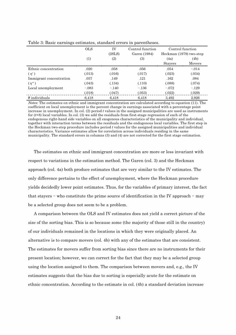
Table 3 reports the results of the basic specification for earnings. The outcome of interest
is defined conditional on having positive earnings. As we go along in Table 3, we add more
sophistication but also more structure. Column (1) reports OLS estimates where we treat
the four local variables as exogenous. Column (2) gives the results of the IV (2SLS)
procedure, which uses the local variables for each immigrant’s initial placement (in year t)
as instruments for current (year t+8) local conditions.32 In column (3), we present the
results from a control function approach due to Garen (1984). The value of this approach
relative to IV is that it allows ])([ 0iii mmE ββ − to depend on 0
im .33 Column (4), finally,
presents the result of the Heckman (1979) two-step estimator; we choose the two-step
estimator, rather than the FIML estimator, since the former is more robust to departures
from bivariate normality.
According to the OLS estimates we are led to believe that ethnic and immigrant
concentration do not matter for earnings. Unemployment is the only local variable that is
of importance (in the statistical sense) for earnings. A standard deviation increase in
ethnic concentration is associated with an (insignificant) earnings gain of 1.4 percent. 34
The IV estimates, however, imply that these conclusions are premature, since the OLS
estimates on ethnic and immigrant concentration are downward biased by a factor of three
to four.35 Interestingly, the precision of ethnic concentration is not much affected by the
IV-procedure. In this instance, a standard deviation rise in ethnic concentration produces
a significant earnings increase of 4.2 percent.
32 Estimates where municipal house prices were used as an additional instrument are almost identical to those reported here. 33 It adds the assumption that the conditional expectations of the individual specific error terms ( αα −i and ββ −i ) can be written as linear functions of the local variables in t + 8 and t; see Card (1999). 34 The standard deviation is calculated within ethnic groups. 35 A Hausman test of the exogeneity of the local variables decisively rejects exogeneity. The test statistic is F(4, 249) = 7.47 (degrees of freedom within parentheses), with a p-value of 0.000.
24
Table 3: Basic earnings estimates, standard errors in parentheses. OLS IV
(2SLS) Control function
Garen (1984) Control function
Heckman (1979) two-step (1) (2) (3) (4a)
Stayers (4b)
Movers
Ethnic concentration ( eη )
.020 (.013)
.058 (.016)
.056 (.017)
.054 (.023)
−.014 (.034)
Immigrant concentration ( mη )
.037 (.043)
.149 (.134)
.121 (.110)
.162 (.088)
.084 (.074)
Local unemployment −.083 (.018)
−.140 (.047)
−.136 (.053)
−.072 (.022)
−.129 (.029)
# individuals 6,418 6,418 6,418 3,492 2,926 Notes: The estimates on ethnic and immigrant concentration are calculated according to equation (11). The coefficient on local unemployment is the percent change in earnings associated with a percentage point increase in unemployment. In col. (2) period t values in the assigned municipalities are used as instruments for (t+8) local variables. In col. (3) we add the residuals from first-stage regression of each of the endogenous right-hand side variables on all exogenous characteristics of the municipality and individual, together with interaction terms between the residuals and the endogenous local variables. The first step in the Heckman two-step procedure includes period t values for the assigned municipalities and individual characteristics. Variance estimates allow for correlation across individuals residing in the same municipality. The standard errors in columns (3) and (4) are not corrected for the first stage estimation.
The estimates on ethnic and immigrant concentration are more or less invariant with
respect to variations in the estimation method. The Garen (col. 3) and the Heckman
approach (col. 4a) both produce estimates that are very similar to the IV estimates. The
only difference pertains to the effect of unemployment, where the Heckman procedure
yields decidedly lower point estimates. Thus, for the variables of primary interest, the fact
that stayers − who constitute the prime source of identification in the IV approach − may
be a selected group does not seem to be a problem.
A comparison between the OLS and IV estimates does not yield a correct picture of the
size of the sorting bias. This is so because some (the majority of those still in the country)
of our individuals remained in the locations in which they were originally placed. An
alternative is to compare movers (col. 4b) with any of the estimates that are consistent.
The estimates for movers suffer from sorting bias since there are no instruments for their
present location; however, we can correct for the fact that they may be a selected group
using the location assigned to them. The comparison between movers and, e.g., the IV
estimates suggests that the bias due to sorting is especially acute for the estimate on
ethnic concentration. According to the estimate in col. (4b) a standard deviation increase

25
in ethnic concentration decreases earnings by 1.0 percent.36
A word of caution should accompany the control function estimates in column (4) since
they rely on functional form to a great deal. Although our equations are identified without
the non-linear transformation of the inverse Mill’s ratio, some experimentation with a
linear selection term (Olsen, 1980) results in imprecise estimates of the coefficients on the
local variables, which suggests that “true” identification is weak.37 Therefore, we drop the
selection correction approach from here on and resort to the simpler control function
approach of Garen, which seems to be less demanding of the data in this setting.
Throughout the analysis we have assumed that the initial location does not affect
current income. An important issue is whether this exclusion restriction is valid. To
examine this issue we have performed Sargan tests of overidentifying restrictions on
slight variations of our basic model. Since our baseline specification is exactly identified
we cannot apply the Sargan procedure directly. Therefore, we amended the instrument set
by including the lags of the original instruments. In general, the parameters of interest
were not affected by altering the set of instruments. Furthermore, the Sargan-statistics do
not reject the estimated models. This result lends support to the identifying assumption
that initial location does not have a permanent effect on earnings.
To sum up this subsection, we have two major findings. First, there is pervasive
evidence that estimates of ”neighborhood” effects that do not account for sorting may be
severely biased.38 Our results indicate that high (unobservable) ability immigrants locate
outside ethnic enclaves to a greater extent. Second, and perhaps more importantly,
immigrants derive a (statistically significant) positive return from living in ethnic
enclaves. There is an earnings gain of four percent associated with a standard deviation
increase in ethnic concentration. We interpret this result as being consistent with
hypotheses stressing that ethnic enclaves may be associated with, e.g., positive network
effects.
36 A simple OLS regression for movers yields a slightly greater earnings reduction. 37 We have tried adding local variables as well as interactions between individual characteristics and local variables to the selection equation with essentially the same result. 38 In this sense, our results are similar to Evans et al. (1992), where the neighborhood referred to schools. Our estimates suggest that sorting is pervasive even when using a more extensive measure of a neighborhood.
26
Idleness
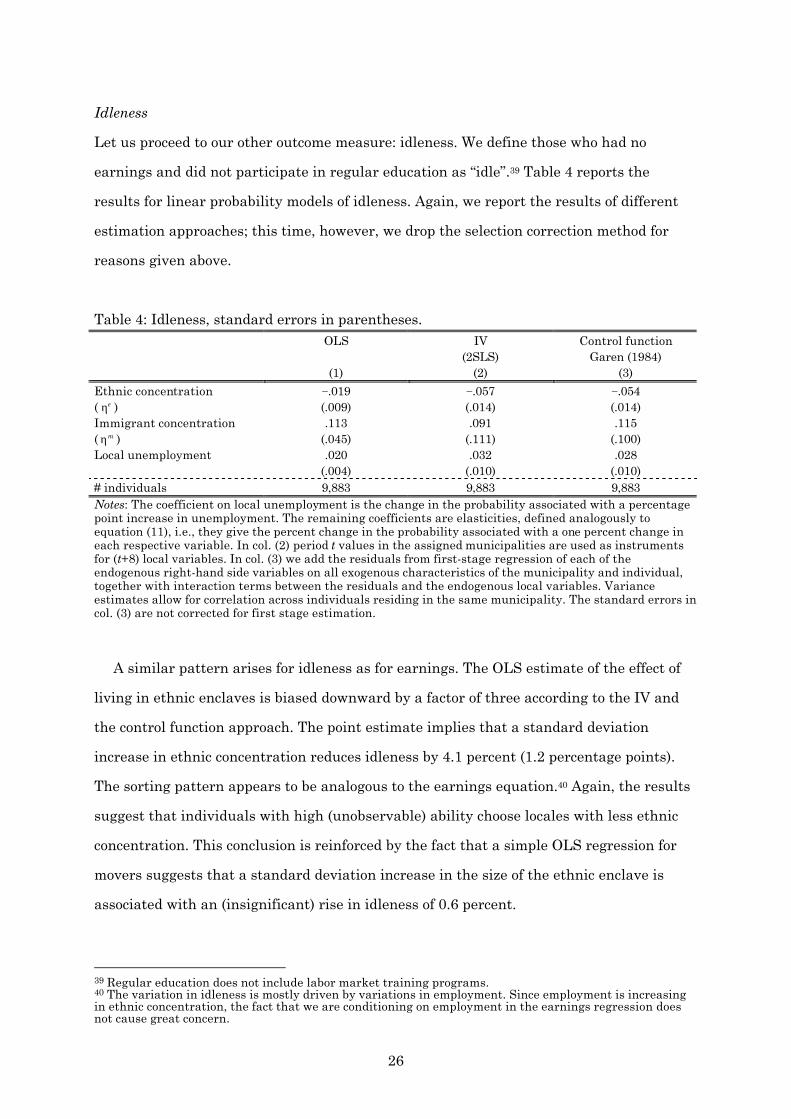
Let us proceed to our other outcome measure: idleness. We define those who had no
earnings and did not participate in regular education as “idle”.39 Table 4 reports the
results for linear probability models of idleness. Again, we report the results of different
estimation approaches; this time, however, we drop the selection correction method for
reasons given above.
Table 4: Idleness, standard errors in parentheses. OLS IV
(2SLS) Control function
Garen (1984) (1) (2) (3)
Ethnic concentration ( eη )
−.019 (.009)
−.057 (.014)
−.054 (.014)
Immigrant concentration ( mη )
.113 (.045)
.091 (.111)
.115 (.100)
Local unemployment .020 (.004)
.032 (.010)
.028 (.010)
# individuals 9,883 9,883 9,883 Notes: The coefficient on local unemployment is the change in the probability associated with a percentage point increase in unemployment. The remaining coefficients are elasticities, defined analogously to equation (11), i.e., they give the percent change in the probability associated with a one percent change in each respective variable. In col. (2) period t values in the assigned municipalities are used as instruments for (t+8) local variables. In col. (3) we add the residuals from first-stage regression of each of the endogenous right-hand side variables on all exogenous characteristics of the municipality and individual, together with interaction terms between the residuals and the endogenous local variables. Variance estimates allow for correlation across individuals residing in the same municipality. The standard errors in col. (3) are not corrected for first stage estimation.
A similar pattern arises for idleness as for earnings. The OLS estimate of the effect of
living in ethnic enclaves is biased downward by a factor of three according to the IV and
the control function approach. The point estimate implies that a standard deviation
increase in ethnic concentration reduces idleness by 4.1 percent (1.2 percentage points).
The sorting pattern appears to be analogous to the earnings equation.40 Again, the results
suggest that individuals with high (unobservable) ability choose locales with less ethnic
concentration. This conclusion is reinforced by the fact that a simple OLS regression for
movers suggests that a standard deviation increase in the size of the ethnic enclave is
associated with an (insignificant) rise in idleness of 0.6 percent.
39 Regular education does not include labor market training programs. 40 The variation in idleness is mostly driven by variations in employment. Since employment is increasing in ethnic concentration, the fact that we are conditioning on employment in the earnings regression does not cause great concern.

27
6.3 Are the basic earnings estimates stable?
The baseline earnings estimates presented above are associated with some potential
problems related to model specification and particular features of the data. We have two
main issues in mind. First, the models are estimated using a parsimonious set of local
variables. It may be the case that the effect of ethnic concentration just stems from some
omitted local variable correlated with ethnic concentration. Second, we do not observe
actual placements of refugees. For example, we know that only 90 percent of the refugee
immigrants were actually subjected to the placement policy. Furthermore, if refugees
move within the year of receiving residence permits, we do not observe their municipality
of placement (since we only observe residence at the end of the year). Thus, our
instruments are not valid for all observations in our sample.
In Table 5 we assess the stability of the key parameter by various ways of accounting
for these problems. We start by investigating whether the effect of ethnic concentration is
driven by omitted local characteristics. First, we increased the set of local variables by
including a proxy for local prices (house prices) and the share of employment in
manufacturing; see row (2). This permutation did not have much effect on the estimates;
moreover, the added local variables did not enter significantly in the estimated
relationship. Second, we added the mean earnings of non-OECD immigrants with similar
results (row (3)). Third, we included a set of (23) county dummies to capture other omitted
regional characteristics (row (4)). The results were almost identical to the baseline
estimates. This set of additional estimates makes us confident that it really is ethnic
concentration that drives our results.

28
Table 5: Stability of the elasticity of ethnic concentration.
Variation Elasticity Standard error
(1) Baseline estimate .058 (.016)
Alternating the set of controls
(2) Add house prices and industry structure .055 (.016) (3) Add mean earnings in municipality, non-OECD immigrants .057 (.016) (4) Add county dummies .057 (.017) (5) Delete schooling variable .046 (.017)
Weighting (to conform to municipal distribution of other data)
(6) Immigration Board, municipal placement .083 (.022) (7) Total inflow of refugees .073 (.020) (8) 1–p, where p is pre-reform distribution (81/83 immigrants) .059 (.017)
Restrictions on the sample
(9) Delete top 8 percent of initial earnings distribution (to conform to aggregate statistics on immigrant inflow)
.060 (.018)
(10) Only individuals from countries listed as refugee source countries by the Immigration Board
.066 (.024)
(11) 1989 immigrants only (most likely to be exogenously placed) .056 (.037) (12) Delete top 10 percent in residual earnings distribution (check if estimate
is driven by high ability individuals being able to choose preferred location)
.056 (.017)
(13) Delete top 10 percent in residual earnings distribution on the basis of pre-reform distribution (high ability individuals able to choose, choices similar to previous immigrants’)
.067 (.020)
Notes: Entries show the elasticity of earnings with respect to ethnic concentration. The weighting procedure (used in variations under “Weighting”) gives higher weight to observations initially in municipalities where the probability is higher that the individual was placed by the government. All local variables are treated as endogenous. The regressions were estimated by IV (2SLS); the instrumentation is explained in Table 3. For (12) and (13), we predict residuals from an OLS earnings regression like the one in Table A2, but without local variables.
We now turn to the potential problems related to our data. Since we lack information
on the individual’s refugee status, it is natural to ask whether this produces a significant
bias in our estimates. Of course, we cannot settle this issue completely, but this section
reports some evidence suggesting that this problem does not cause great concern.
By comparing the number of individuals in our sample with the total number of
allotted residence permits during 1987 to 1989, we conclude that we sample too many
individuals. This leads to the suspicion that some of our individuals may have immigrated
for other reasons than political and, hence, were not assigned a municipality by the
Immigration Board. In particular, some of our individuals may have immigrated for labor
market reasons.
We approached this problem in two ways. The first approach is to use information on
the number of received refugee immigrants in each municipality. We reweigh our data

29
such that the distribution of the initial locations of the individuals in our sample
corresponds to the distribution of received refugees over municipalities. One weighting
procedure is based on the number of refugees covered by grants from the Immigration
Board (row (6)). Thereby, we can also address the problem that some individuals may
already have relocated from the assigned municipality when we first observe them. As an
alternative (row (7)), we use the distribution of initial locations from individual data in
another dataset (FLYDATA; see Rooth (1999)). Both these weighted estimates of ethnic
concentration are higher than the baseline estimate.
A second way to handle the lack of data on individuals’ refugee status is restricting the
sample. One idea is that those with the highest earnings during the year of immigration
(period t) are least likely to be refugees; this appears a plausible assumption given that
refugees could live on welfare during their initial period in Sweden. So, we excluded
individuals at the top end of the period t earnings distribution until the number of
sampled individuals was conformable with aggregate statistics (row (9)). This exclusion
produced a reduction of the earnings sample by 8 percent, leaving the estimate of ethnic
concentration essentially unchanged.
Moreover, we have also restricted the sample to individuals arriving from countries
listed as refugee source countries by the Immigration Board (row (10)). This restriction
eliminates a number of small countries in terms of immigrant inflow and produces a
somewhat higher estimate of the effect of ethnic concentration than the baseline estimate.
Thus we conclude that, if anything, the fact that we do not observe refugee status tends to
bias our estimates of the causal effect of living in enclaves downwards.
A related problem with our data is the fact that we do not observe which individuals
were subjected to the placement policy. We know that about ten percent of refugees chose
not to participate in the program, and there is a possibility that some refugees were able
to influence their placement. We have tried various ways to assess whether this may bias
our estimates.41
Our first attempt to alleviate this problem is based on the assumption that, in the
41 To test whether the missing information on placement in combination with the estimation approach yields an upward bias in the estimates, we used a “fake” IV procedure. We applied our IV approach to the pre-program cohort (1981/83). OLS and IV applied to this cohort should give the same estimates. This turned out to be the case.
30
absence of the placement program, refugees would have behaved similarly to previous
refugee immigrants. Consequently, we use the pre-program distribution of initial location
in weighting the estimates (row (8)). Municipalities that received a large share of
immigrants in the 1981/83 cohort, are weighted down relative to municipalities that
received few immigrants. The results are not affected by this weighting procedure.
Another way to try to get at the effects of missing information on placement is to
restrict the sample to those who received their residence permits in 1989. This was when
the placement policy was most restrictive. Also in this case, the point estimates are
virtually identical in comparison with the full sample; see row (11).
The above two robustness checks are based on the assumption that the probability of
being treated (placed) is independent of unobserved characteristics. This is a strong
assumption. A reasonable hypothesis may be that the skilled (in a general sense) are more
able to influence their placement than the unskilled. What does this hypothesis imply for
our estimates? One approach to this question is to delete the educational dummies from
the set of individual controls. The idea is that if the probability of influencing placement is
similarly affected by unobserved and observed skills (i.e. schooling), dropping education
provides information on the sign of the omitted variable bias. The result of this
experiment is that the estimate on ethnic concentration drops somewhat; see row (6). This
suggests that there is no upward bias as a result of the fact that those with plenty of
unobserved skills may have been able to influence their placement.
Another approach to get a handle of the bias resulting from unobserved skills
influencing placement, is to drop the top of the residual earnings distribution. We have
explored two variants of this approach. First, we dropped the top ten percent of the overall
residual distribution (row (12)). Second, under the assumption that the choices of location
would have been similar to previous refugees, we dropped the top ten percent using the
pre-reform distribution of municipalities as weights (row (13)). These two sample
restrictions gave estimates that were similar and somewhat higher, respectively,
compared to the baseline estimates.
In summary, we have performed a large number of robustness checks and find the basic
estimates to be stable. If anything, the baseline estimates probably understate the true
effect of ethnic concentration.

31
6.4 Does the return to living in an enclave vary across groups?
Our approach to answering this question is to interact measures of skill with local
characteristics. We have considered interactions with gender, individual education and
region of origin. We found no differences across region of origin, nor between males and
females.42 There were some interesting differences across educational groups however.
Table 6 presents estimates for various educational groups, analogous to those in Table
3. The effect of ethnic concentration exhibits an interesting pattern. The positive effect of
living in an enclave declines monotonously with observable skill until we reach the
university level. For individuals with the highest education we also estimate a positive
(and significant) effect. It is possible that the latter result is due to cream skimming by
municipal officers (although our previous evidence does not suggest that this is a major
issue). Due to this potential problem and the relative magnitude of the estimated effects,
we are inclined to interpret the results in Table 6 as saying that the least skilled are the
ones who gain most from living in ethnic enclaves.43 This is consistent with a story that
emphasizes that enclaves are associated with ethnic networks who primarily benefits the
least skilled.
42 The estimate of the elasticity of earnings with respect to ethnic concentration was 0.055 for males and 0.065 for females, with standard errors of 0.023 and 0.025, respectively. 43 Interestingly, this is also the group that gains the least from language acquisition, according to Berman et al. (2000).

32
Table 6: The effect of local characteristics by education, standard errors in parentheses Educational level missing &
< 9 years 9–10 years
high school
≤ 2 years high school
> 2 years university < 3 years
university ≥ 3 years
Ethnic concentration ( eη )
.156 (.039)
.123 (.034)
.037 (.035)
−.067 (.042)
.051 (.044)
.092 (.044)
Immigrant concentration ( mη )
.250 (.210)
−.310 (.162)
.288 (.197)
.225 (.237)
.398 (.386)
−.018 (.353)
Local unemployment −.021 (.065)
−.211 (.087)
−.129 (.063)
−.150 (.070)
−.229 (.103)
−.070 (.120)
# individuals 1,041 1,170 1,220 1,222 922 843 Notes: All regressions were estimated by IV (2SLS). Local variables are instrumented as explained in Table 3. Robust variance estimates, allowing for correlation across individuals residing in the same municipality.
7. Concluding remarks
The main purpose of this paper has been to provide estimates of the causal effect on
economic outcomes of living in an enclave. To this end, we have made use of an immigrant
policy initiative in Sweden, when government authorities distributed refugee immigrants
across locales in a way that may be considered as exogenous. This policy initiative
provides a unique natural experiment, which allows us handle the endogeneity problem
due to individuals’ choice of residence.
Our empirical analysis suggests two principal conclusions. First, we find evidence of
sorting across locations. There is a substantive downward bias in estimates that do not
account for sorting. Second, and perhaps more importantly, when accounting for the
endogeneity of residential choice we find that an increase in ethnic concentration gives
rise to a (statistically significant) improvement in labor market outcomes (earnings and
idleness). For instance, the earnings gain associated with a standard deviation increase in
ethnic concentration is in the order of four to five percent. Further, these gains appear to
be concentrated in the lower end of the observable skill distribution.
We have offered evidence suggesting that ethnic enclaves contribute to an increase in
the level of earnings. This is consistent with the view that the enclave offers a “warm
embrace”, helping immigrants escape the discrimination encountered elsewhere on the
labor market. Another issue is whether enclaves also contribute to earnings assimilation,
i.e., to the rate of change in earnings. It may well be that the warm embrace is too
comfortable so that incentives to move upwards on the job-ladder are reduced. Recent
evidence presented in Borjas (2000) suggests that this indeed is the case: enclaves decrease

33
immigrant assimilation. However, this evidence potentially suffers from the Tiebout bias
that we have addressed.
Finally, let us note that we have not exploited the full potential of the data. Our
analysis has been based on rather broad geographical units. But ethnic segregation may
vary a great deal within these broader units. During the years of the settlement policy,
refugee immigrants were actually placed directly in an apartment. This fact gives ample
scope for utilizing information on finer geographical units, such as housing blocks.
The questions of whether ethnic clustering affects immigrant assimilation and the
consequences of housing segregation for individual outcomes are of substantial interest.
We have put these issues on our research agenda.
34
References
Angrist, J.D. (1990), “Lifetime Earnings and the Vietnam Era Draft Lottery: Evidence from Social Security Administrative Records”, American Economic Review 80, 313–336.
Angrist, J.D., G.W. Imbens, and D.B. Rubin (1996), “Identification of Causal Effects Using Instrumental Variables”, Journal of the American Statistical Association 91, 444–472.
Bartel, A.P. (1989), ”Where Do the New U.S. Immigrants Live?”, Journal of Labor Economics 7(4), 371–391.
Berman, E., K. Lang, and Erez Siniver (2000), “Language-Skill Complementarity: Returns to Immigrant Language Acquisition”, NBER Working Paper 6832.
Bertrand, B., E.F.P. Luttmer, and S. Mullainathan (2000), “Network Effects and Welfare Cultures”, Quarterly Journal of Economics 115(3), 1019–1055.
Borjas, G.J. (1994), ”The Economics of Immigration”, Journal of Economic Literature XXXII, 1667–1717.
Borjas, G.J. (1995), “Ethnicity, Neighborhoods, and Human-Capital Externalities”, American Economic Review, 85(3), 365–390.
Borjas, G.J. (1998), ”To Ghetto or Not to Ghetto: Ethnicity and Residential Segregation”, Journal of Urban Economics 44, 228–253.
Borjas, G.J. (1999), Heaven’s Door – Immigration Policy and the American Economy, Princeton University Press, Princeton.
Borjas, G.J. (2000), “Ethnic Enclaves and Immigrant Assimilation”, paper prepared for the Economic Council of Sweden’s conference on “The Economic Assimilation of Immigrants in the Labour Market”, Stockholm.
Card, D., (1999), “The Causal Effect of Education on Earnings”, in O. Ashenfelter and D. Card (eds.), Handbook of Labor Economics vol. 3, North-Holland, Amsterdam.
Cutler, D.M. and E.L. Glaeser (1997), “Are Ghettos Good or Bad?” Quarterly Journal of Economics 112 (3), 827–872.
Dustmann C. and I. Preston (1998), ”Attitudes to Ethnic Minorities, Ethnic Context and Location Decision”, CEPR Discussion Paper No. 1942.
Edin, P-A. and P. Fredriksson (2000), ”LINDA – Longitudinal INdividual DAta for Sweden”, Working Paper 2000:19, Department of Economics, Uppsala University.
Evans, W.N., W.E. Oates, and R.M. Schwab (1992), ”Measuring Peer Group Effects: A Study of Teenage Behavior”, Journal of Political Economy 100, 966–991.
Gabriel, S.A. and S.S. Rosenthal (1999), ”Location and the Effect of Demographic Traits on Earnings”, Regional Science and Urban Economics 29, 445–461.
Garen, J. (1984), “The Returns to Schooling: A Selectivity Bias Approach with a Continuous Choice Variable”, Econometrica 52, 1199–1218.
Greenwood, M.J. (1997), ”Internal Migration in Developed Countries”, in M.R. Rosenzweig and O. Stark (eds.), Handbook of Population Economics, North-Holland.
Heckman, J.J. (1979), “Sample Selection Bias as a Specification Error”, Econometrica 47, 153–161.
Heckman, J.J. (1997), “Instrumental Variables: A Study of Implicit Behavioral Assumptions Used in Making Program Evaluations”, Journal of Human Resources 32, 441–462.
Heckman, J.J. and R.R Robb Jr. (1985), “Alternative Methods for Evaluating the Impact of Interventions”, in J.J. Heckman and B. Singer (eds.), Longitudinal Analysis of Labor Market Data, Econometric Society Monographs series, no. 10, Cambridge University Press, 156–245.
Ihlanfeldt, K.R. and D.L. Sjoquist (1998), “The Spatial Mismatch Hypothesis: A Review of Recent Studies and Their Implications for Welfare Reform”, Housing Policy Debate 9(4), 849–892.

35
Kain, J. (1968), ”Housing Segregation, Negro Employment, and Metropolitan Decentralization”, Quarterly Journal of Economics LXXXII, 175–197.
Katz, L.F, J.R. Kling, and J.B. Liebman (2000), “Moving to Opportunity in Boston: Early Results of a Randomized Mobility Experiment”, Working Paper #441, Princeton University, Industrial Relations Section.
LaLonde, R.J and R.H. Topel (1991), ”Labor Market Adjustments to Increased Immigration”, in J.M. Abowd and R.B. Freeman (eds.), Immigration, Trade, and the Labor Market, University of Chicago Press.
LaLonde, R.J and R.H. Topel (1997), ”Economic Impact of International Migration and the Economic Performance of Migrants”, in M.R. Rosenzweig and O. Stark (eds.), Handbook of Population Economics, North-Holland.
Manski, C.F. (1993), ”Identification of Endogenous Social Effects: The Reflection Problem”, Review of Economic Studies 60, 531–542.
Olsen, R.J., (1980), “A Least Squares Correction for Selectivity Bias”, Econometrica 48, 1815–1820.
Portes, A. (1987), “The Social Origins of the Cuban Enclave Economy of Miami”, Sociological Perspectives 30(4), 340–372.
Rooth, D-O. (1999), Refugee Immigrants in Sweden – Educational Investments and Labour Market Integration, PhD thesis, Lund Economic Studies number 84, Department of Economics, University of Lund.
The Immigration Board (1997), Individuell mångfald: Invandrarverkets utvärdering och analys av det samordnade flyktingmottagandet 1991–1996, Statens invandrarverk.
The Committee on Immigration Policy (1996), Sverige, framtiden och mångfalden. Slutbetänkande från Invandrarpolitiska kommittén, SOU 1996:55, Fritzes, Stockholm.
Wooldridge, J.M. (1997), “On Two Stage Least Squares Estimation of the Average Treatment Effect in a Random Coefficient Model”, Economics Letters 56, 129–133.
Åslund, O. (2000), “Immigrant Settlement Policies and Subsequent Migration”, mimeo, Department of Economics, Uppsala University.

36
Appendix
Table A1: Summary statistics Total sample
(# individuals: 9,883) Earnings sample
(# individuals: 6,418) Variable Mean Std. Dev. Mean Std. Dev.
Local characteristics ln (ethnic group) ( eln ) 5.252 2.110 5.104 2.111 ln (other immigrants) ( mln ) 9.061 1.575 8.954 1.601 ln (natives) ( nln ) 11.619 1.226 11.534 1.247 Unemployment rate (percent) 5.885 1.391 5.825 1.404 Ethnic concentration ( )( mene ++ )*102
(standard deviation within country) .3478 .4016
(.2424) .3304 .3932
(.2401) Immigrant concentration ( )( menm ++ )*102 7.880 3.275 7.761 3.339 Individual characteristics Earnings -- -- 10.955 1.513 Idleness .292 .455 -- -- Welfare dependency .321 .467 -- -- Stayer .538 .499 .544 .498 Female .445 .497 .447 .497 Age 38.124 8.289 37.437 7.506 Married .592 .492 .624 .484 Kid .514 .500 .560 .496 Education: Missing and < 9 years .214 .410 .162 .369 9–10 years .185 .388 .182 .386 High school ≤ 2 years .168 .374 .190 .392 High school > 2 years .185 .388 .190 .393 University < 3 years .134 .341 .144 .351 University ≥ 3 years .114 .317 .131 .338 Region of origin: Eastern Europe .180 .384 .201 .401 Africa .116 .320 .117 .321 Middle East .457 .498 .403 .490 Asia .083 .277 .089 .284 South America .164 .370 .190 .393 Immigration year: 1987 .260 .439 .276 .447 1988 .355 .478 .357 .479 1989 .385 .487 .367 .482
Notes: All variables refer to the situation in t+8. Entries for local variables under the heading “Total sample” are population weighted. Entries for local variables under the heading “Earnings sample” are employment weighted. The “standard deviation within country” for ethnic concentration is a weighted average of the standard deviations within each country of origin.

37
Table A2: Basic OLS and IV estimates, standard errors in parentheses. ln(earnings)|
earnings>0 Pr(idle)
(1) OLS
(2) IV
(3) OLS
(4) IV
Panel a) ln(ethnic group)
.020
(.013)
.057
(.016)
−.006 (.003)
−.017 (.004)
ln(other immigrants) .030 (.039)
.135 (.121)
.032 (.012)
.026 (.029)
ln(natives) −.085 (.063)
−.161 (.150)
−.012 (.015)
−.001 (.044)
Unemployment rate −.083 (.018)
−.140 (.047)
.020 (.004)
.032 (.010)
Panel b) Female
.034
(.070)
.032
(.071)
−.003 (.024)
−.002 (.024)
Age .052 (.022)
.055 (.022)
−.015 (.005)
−.016 (.005)
Age squared (*10-2) −.057 (.027)
−.061 (.027)
.030 (.006)
.030 (.006)
Married .239 (.068)
.244 (.071)
−.077 (.018)
−.076 (.019)
Kid −.062 (.058)
−.031 (.058)
−.041 (.013)
−.045 (.013)
Married*female −.128 (.085)
−.105 (.085)
.033 (.021)
.029 (.022)
Kid*female −.305 (.095)
−.324 (.098)
−.028 (.023)
−.025 (.023)
Education (missing and < 9 years, ref.) 9–10 years .059
(.056) .051
(.055) −.113 (.014)
−.111 (.014)
High school ≤ 2 years .184 (.082)
.179 (.082)
−.185 (.013)
−.183 (.013)
High school > 2 years .191 (.062)
.175 (.064)
−.162 (.014)
−.158 (.015)
University < 3 years .110 (.065)
.090 (.066)
−.253 (.019)
−.249 (.018)
University ≥ 3 years .479 (.086)
.464 (.088)
−.238 (.013)
−.236 (.014)
Region of origin (Eastern Europe, ref.) Africa −.197
(.110) −.211 (.111)
.030 (.020)
.023 (.024)
Middle East −.544 (.061)
−.592 (.074)
.112 (.012)
.122 (.013)
Asia −.021 (.085)
−.007 (.088)
.017 (.016)
.006 (.018)
South America −.036 (.054)
−.050 (.056)
−.056 (.020)
−.054 (.021)
Immigration year (1987, ref.) 1988 −.102
(.041) −.119 (.050)
.053 (.009)
.057 (.011)
1989 −.145 (.044)
−.193 (.081)
.101 (.014)
.113 (.014)
# individuals
6,418
6,418
9,883
9,883
R-squared .063 .054 .120 .118
Notes: IV estimation by 2SLS using values in the assigned municipalities as instruments for (t+8) local variables. Robust variance estimates, allowing for correlation across individuals residing in the same municipality.

38