et and 3g science

ET and 3G ScienceStephen Fairhurst

1

The birth of GW astronomy

2

The birth of GW astronomy• Observation of Gravitational

waves from a BBH merger

GW150914

2



• Tests of General Relativity

2

charges, one should directly apply full inspiral-merger-ringdown waveform models from specific modified gravitytheories [147], but in most cases, these are not yet available.However, in the present work, the focus is on model-independent tests of general relativity itself.Given the observation of more than one BBH merger,

posterior distributions for the δpi can be combined to yieldstronger constraints. In Fig. 7, we show the posteriors fromGW150914, generated with final instrumental calibration,and GW151226 by themselves, as well as joint posteriorsfrom the two events together. We do not present similarresults for the candidate LVT151012 since it is not asconfident a detection as the others; furthermore, its smallerdetection SNR means that its contribution to the overallposteriors is insignificant.For GW150914, the testing parameters for the PN

coefficients, δφi and δφil, showed moderately significant(2σ–2.5σ) deviations from their general relativity values ofzero [41]. By contrast, the posteriors of GW151226 tend tobe centered on the general relativity value. As a result, theoffsets of the combined posteriors are smaller. Moreover,the joint posteriors are considerably tighter, with a 1σspread as small as 0.07 for deviations in the 1.5PNparameter φ3, which encapsulates the leading-order effectsof the dynamical self-interaction of spacetime geometry(the “tail” effect) [148–151], as well as spin-orbit inter-action [67,152,153].In Fig. 8, we show the 90% credible upper bounds on the

magnitude of the fractional deviations in PN coefficients,jδφij, which are affected by both the offsets and widths ofthe posterior density functions for the δφi. We show bounds

for GW150914 and GW151226 individually, as well as thejoint upper bounds resulting from the combined posteriordensity functions of the two events. Not surprisingly, thequality of the joint bounds is mainly due to GW151226because of the larger number of inspiral cycles in thedetectors’ sensitive frequency band. Note how at high PNorder, the combined bounds are slightly looser than theones from GW151226 alone; this is because of the largeoffsets in the posteriors from GW150914.Next, we consider the intermediate-regime coefficients

δβi, which pertain to the transition between inspiral andmerger-ringdown. For GW151226, this stage is well insidethe sensitive part of the detectors’ frequency band.Returning to Fig. 7, we see that the measurements forGW151226 are of comparable quality to GW150914, andthe combined posteriors improve on the ones from eitherdetection by itself. Last, we look at the merger-ringdownparameters δαi. For GW150914, this regime correspondedto frequencies of f ∈ ½130; 300" Hz, while for GW151226,it occurred at f ≳ 400 Hz. As expected, the posteriors fromGW151226 are not very informative for these parameters,and the combined posteriors are essentially determined bythose of GW150914.In summary, GW151226 makes its most important

contribution to the combined posteriors in the PN inspiralregime, where both offsets and statistical uncertainties havesignificantly decreased over the ones from GW150914, insome cases almost to the 10% level.An inspiral-merger-ringdown consistency test as per-

formed on GW150914 in Ref. [41] is not meaningful forGW151226 since very little of the signal is observed in thepost-merger phase. Likewise, the SNR of GW151226 is toolow to allow for an analysis of residuals after subtraction ofthe most probable waveform. In Ref. [41], GW150914 wasused to place a lower bound on the graviton Comptonwavelength of 1013 km GW151226 gives a somewhatweaker bound because of its lower SNR, so combininginformation from the two signals does not significantlyimprove on this; an updated bound must await furtherobservations. Finally, BBH observations can be used to testthe consistency of the signal with the two polarizations ofgravitational waves predicted by general relativity [154].However, as with GW150914, we are unable to test thepolarization content of GW151226 with the two, nearlyaligned aLIGO detectors. Future observations, with anexpanded network, will allow us to look for evidence ofadditional polarization content arising from deviations fromgeneral relativity.

VI. BINARY BLACK HOLE MERGER RATES

The observations reported here enable us to constrain therate of BBH coalescences in the local Universe moreprecisely than was achieved in Ref. [42] because of thelonger duration of data containing a larger number ofdetected signals.

FIG. 8. The 90% credible upper bounds on deviations in the PNcoefficients, from GW150914 and GW151226. Also shown arejoint upper bounds from the two detections; the main contributoris GW151226, which had many more inspiral cycles in band thanGW150914. At 1PN order and higher, the joint bounds areslightly looser than the ones from GW151226 alone; this is due tothe large offsets in the posteriors for GW150914.

BINARY BLACK HOLE MERGERS IN THE FIRST … PHYS. REV. X 6, 041015 (2016)

041015-17




• Multimessenger observationof a BNS merger

The 90% credible intervals(Veitch et al. 2015; Abbott et al.2017e) for the component masses (in the m m1 2. convention)are m M1.36, 2.261 Î :( ) and m M0.86, 1.362 Î :( ) , with totalmass M2.82 0.09

0.47-+

:, when considering dimensionless spins with

magnitudes up to 0.89 (high-spin prior, hereafter). When thedimensionless spin prior is restricted to 0.05- (low-spin prior,hereafter), the measured component masses are m 1.36,1 Î (

M1.60 :) and m M1.17, 1.362 Î :( ) , and the total mass is

Figure 2. Joint, multi-messenger detection of GW170817 and GRB170817A. Top: the summed GBM lightcurve for sodium iodide (NaI) detectors 1, 2, and 5 forGRB170817A between 10 and 50 keV, matching the 100 ms time bins of the SPI-ACS data. The background estimate from Goldstein et al. (2016) is overlaid in red.Second: the same as the top panel but in the 50–300 keV energy range. Third: the SPI-ACS lightcurve with the energy range starting approximately at 100 keV andwith a high energy limit of least 80 MeV. Bottom: the time-frequency map of GW170817 was obtained by coherently combining LIGO-Hanford and LIGO-Livingston data. All times here are referenced to the GW170817 trigger time T0

GW.

3

The Astrophysical Journal Letters, 848:L13 (27pp), 2017 October 20 Abbott et al.

2





• Cosmology withGW observations

2

LETTERRESEARCH

8 6 | N A T U R E | V O L 5 5 1 | 2 N O V E M B E R 2 0 1 7

by a viewing angle defined as min(ι, 180° − ι), with ι in the range [0°, 180°]. By contrast, gravitational-wave measurements can identify the sense of the rotation, and so ι ranges from 0° (anticlockwise) to 180° (clockwise). Previous gravitational-wave detections by the Laser Interferometer Gravitational-wave Observatory (LIGO) had large uncertainties in luminosity distance and inclination23 because the two LIGO detectors that were involved are nearly co-aligned, preventing a precise polarization measurement. In the present case, owing to the addition of the Virgo detector, the cosine of the inclination can be constrained at 68.3% (1σ) confidence to the range [−1.00, −0.81], corresponding to inclination angles in the range [144°, 180°]. This incli-nation range implies that the plane of the binary orbit is almost, but not quite, perpendicular to our line of sight to the source (ι ≈ 180°), which is consistent with the observation of a coincident γ-ray burst4–6. We report inferences on cosι because our prior for it is flat, so the posterior is proportional to the marginal likelihood for it from the gravitation-al-wave observations.

Electromagnetic follow-up observations of the gravitational-wave sky-localization region7 discovered an optical transient8–13 in close proximity to the galaxy NGC 4993. The location of the transient was previously observed by the Distance Less Than 40 Mpc (DLT40) survey on 27.99 July 2017 universal time (ut) and no sources were found10. We estimate the probability of a random chance association between the optical counterpart and NGC 4993 to be 0.004% (Methods). In what follows we assume that the optical counterpart is associated with GW170817, and that this source resides in NGC 4993.

To compute H0 we need to estimate the background Hubble flow velocity at the position of NGC 4993. In the traditional electro-magnetic calibration of the cosmic ‘distance ladder’19, this step is commonly carried out using secondary distance indicator informa-tion, such as the Tully–Fisher relation25, which enables the back-ground Hubble flow velocity in the local Universe to be inferred by scaling back from more distant secondary indicators calibrated in quiet Hubble flow. We do not adopt this approach here, however, to preserve more fully the independence of our results from the electromagnetic distance ladder. Instead we estimate the Hubble flow velocity at the position of NGC 4993 by correcting for local peculiar motions.

NGC 4993 is part of a collection of galaxies, ESO 508, which has a center-of-mass recession velocity relative to the frame of the cosmic microwave background (CMB)26 of27 3,327 ± 72 km s−1. We correct

the group velocity by 310 km s−1 owing to the coherent bulk flow28,29 towards the Great Attractor (Methods). The standard error on our estimate of the peculiar velocity is 69 km s−1, but recognizing that this value may be sensitive to details of the bulk flow motion that have been imperfectly modelled, in our subsequent analysis we adopt a more conservative estimate29 of 150 km s−1 for the uncertainty on the peculiar velocity at the location of NGC 4993 and fold this into our estimate of the uncertainty on vH. From this, we obtain a Hubble velocity vH = 3,017 ± 166 km s−1.

Once the distance and Hubble-velocity distributions have been determined from the gravitational-wave and electromagnetic data, respectively, we can constrain the value of the Hubble constant. The measurement of the distance is strongly correlated with the measure-ment of the inclination of the orbital plane of the binary. The analy-sis of the gravitational-wave data also depends on other parameters describing the source, such as the masses of the components23. Here we treat the uncertainty in these other variables by marginalizing over the posterior distribution on system parameters3, with the exception of the position of the system on the sky, which is taken to be fixed at the location of the optical counterpart.

We carry out a Bayesian analysis to infer a posterior distribution on H0 and inclination, marginalized over uncertainties in the recessional and peculiar velocities (Methods). In Fig. 1 we show the marginal pos-terior for H0. The maximum a posteriori value with the minimal 68.3% credible interval is = . − .

+ . − −H 70 0 km s Mpc0 8 012 0 1 1. Our estimate agrees

well with state-of-the-art determinations of this quantity, including CMB measurements from Planck20 (67.74 ± 0.46 km s−1 Mpc−1; ‘TT, TE, EE + lowP + lensing + ext’) and type Ia supernova measure-ments from SHoES21 (73.24 ± 1.74 km s−1 Mpc−1), and with baryon acoustic oscillations measurements from SDSS30, strong lensing measurements from H0LiCOW31, high-angular-multipole CMB measurements from SPT32 and Cepheid measurements from the Hubble Space Telescope key project19. Our measurement is an inde-pendent determination of H0. The close agreement indicates that, although each method may be affected by different systematic uncer-tainties, we see no evidence at present for a systematic difference between gravitational-wave-based estimates and established electro-magnetic-based estimates. As has been much remarked on, the Planck and SHoES results are inconsistent at a level greater than about 3σ. Our measurement does not resolve this inconsistency, being broadly consistent with both.

50 60 70 80 90 100 110 120 130 140

H0 (km s–1 Mpc–1)

0.00

0.01

0.02

0.03

0.04

p(H

0 | G

W17

0817

) (km

–1 s

Mpc

)

PlanckSHoES

Figure 1 | GW170817 measurement of H0. The marginalized posterior density for H0, p(H0 | GW170817), is shown by the blue curve. Constraints at 1σ (darker shading) and 2σ (lighter shading) from Planck20 and SHoES21 are shown in green and orange, respectively. The maximum a posteriori value and minimal 68.3% credible interval from this posterior density function is = . − .

+ . − −H 70 0 km s Mpc0 8 012 0 1 1. The 68.3% (1σ) and 95.4%

(2σ) minimal credible intervals are indicated by dashed and dotted lines, respectively.

50 60 70 80 90 100 110 120

H0 (km s–1 Mpc–1)

–1.0

–0.9

–0.8

–0.7

–0.6

–0.5

–0.4

cosL

180170

160

150

140

130

120

L (°)

GW170817PlanckSHoES

Figure 2 | Inference on H0 and inclination. The posterior density of H0 and cosι from the joint gravitational-wave–electromagnetic analysis are shown as blue contours. Shading levels are drawn at every 5% credible level, with the 68.3% (1σ; solid) and 95.4% (2σ; dashed) contours in black. Values of H0 and 1σ and 2σ error bands are also displayed from Planck20 and SHoES21. Inclination angles near 180° (cosι = −1) indicate that the orbital angular momentum is antiparallel to the direction from the source to the detector.

© 2017 Macmillan Publishers Limited, part of Springer Nature. All rights reserved.





• Cosmology withGW observations

• Observing the population of NS and BH

2

Future GW observations• Advance exploration of extremes of gravity and

astrophysics

• Address fundamental questions in physics and astronomy

• Provide insights into most powerful events in the Universe

• Reveal new objects and phenomena

3

3G Committee Structure

3G Committee

Science Case Governance Structure

R&D Coordination

Agency Interfacing

Community Networking

Gravitational-Wave International Committee

neutron stars

seed black holes

detector networks

compact binaries

cosmology supernovamulti-

messenger obs.

extreme gravity

waveform models

3G Committee co-chairs

Punturo, Reitze members

Ferrini, Kajita, Kalogera, Lueck, Marx, McClelland, Rowan, Sathyaprakash,

Shoemaker

for membership of committees see: https://gwic.ligo.org/3Gsubcomm/

4

• Matthew Bailes <[email protected]>

• Marie Anne Bizouard <[email protected]>

• Alessandra Buonanno <[email protected]>

• Adam Burrows <[email protected]>

• Monica Colpi <[email protected]>

• Matt Evans <[email protected]>

• Stephen Fairhurst <[email protected]>

• Stefan.Hild <[email protected]>

• Vicky Kalogera (Co-chair) <[email protected]>

• Mansi M. Kasliwal <[email protected]>,

• Luis Lehner <[email protected]>

• Ilya Mandel <[email protected]>

• Vuk Mandic <[email protected]>

• Marialessandra Papa <[email protected]>

• Sanjay Reddy <[email protected]>

• Stephan Rosswog <[email protected]>

• B.S. Sathyaprakash (Co-chair) <[email protected]>

• Chris Van Den Broeck <[email protected]> 5

3G Science Case Team

6

Working Group Co-chairs

Extreme Gravity Buonanno and Van Den Broeck

Neutron Stars Papa, Reddy, Rosswog

Compact Binaries Bailes, Kalogera, Mandel

Seed Black Holes Colpi, Fairhurst

Supernova Bizouard, Burrows

Cosmology Mandic, Sathyaprakash

Waveforms Buonanno and Lehner

Detector Networks Evans, Fairhurst, Hild

Multi-messenger Observations Bailes, Kasliwal 6

ET and 3G Science Highlights

• Try to identify observations that:

• Will lead to breakthrough science

• Are uniquely available with gravitational wave observations, possibly in conjunction with EM

• Can only be achieved with the sensitivity of 3rd generation detectors such as ET

7

Compact Binaries

8

• What is the mass and spin distribution of compact objects through cosmic time?

100 101 102 103

Total source frame mass [M�]

10�1

100

101

102

Reds

hift

Horizon10% detected50% detected

aLIGOVoyager

ETCE

Credit: Evan Hall

Compact Binaries

9

from the ratio of FIR to observed (uncorrected) FUV luminosity densities (Figure 8) as a

function of redshift, using FUVLFs from Cucciati et al. (2012) and Herschel FIRLFs fromGruppioni et al. (2013). At z < 2, these estimates agree reasonably well with the measure-

ments inferred from the UV slope or from SED fitting. At z > 2, the FIR/FUV estimates

have large uncertainties owing to the similarly large uncertainties required to extrapolatethe observed FIRLF to a total luminosity density. The values are larger than those for

the UV-selected surveys, particularly when compared with the UV values extrapolated to

very faint luminosities. Although galaxies with lower SFRs may have reduced extinction,purely UV-selected samples at high redshift may also be biased against dusty star-forming

galaxies. As we noted above, a robust census for star-forming galaxies at z ≫ 2 selectedon the basis of dust emission alone does not exist, owing to the sensitivity limits of past

and present FIR and submillimeter observatories. Accordingly, the total amount of star

formation that is missed from UV surveys at such high redshifts remains uncertain.

Figure 9: The history of cosmic star formation from (top right panel) FUV, (bottom right panel) IR,and (left panel) FUV+IR rest-frame measurements. The data points with symbols are given in Table1. All UV luminosities have been converted to instantaneous SFR densities using the factor KFUV =1.15 × 10−28 (see Equation 10), valid for a Salpeter IMF. FIR luminosities (8–1,000µm) have beenconverted to instantaneous SFRs using the factor KIR = 4.5 × 10−44 (see Equation 11), also valid for aSalpeter IMF. The solid curve in the three panels plots the best-fit SFRD in Equation 15.

Figure 9 shows the cosmic SFH from UV and IR data following the above prescriptions,

as well as the best-fitting function

ψ(z) = 0.015(1 + z)2.7

1 + [(1 + z)/2.9]5.6M⊙ year−1 Mpc−3. (15)

These state-of-the-art surveys provide a remarkably consistent picture of the cosmic SFH:

a rising phase, scaling as ψ(z) ∝ (1 + z)−2.9 at 3 ∼< z ∼

< 8, slowing and peaking at somepoint probably between z = 2 and 1.5, when the Universe was ∼ 3.5 Gyr old, followed by

48 P. Madau & M. Dickinson

A&A 594, A97 (2016)

0

20

40

60

80

100

20 40 60 80 100 120 140

0

20

40

60

80

100

Fig. 2. Initial-final mass relation for single stars. Models with (M10) andwithout (M1) pair-instability pulsation supernovae and pair-instabilitysupernovae are shown. Bottom panel: at high metallicity (Z = 10% Z�and higher) the models are indistinguishable. For the border-line metal-licity of Z = 10% Z�, stars with very high initial mass (Mzams >100 M�) will form slightly lighter BHs (by ⇠2 M�) if pair-instabilitypulsation supernovae are included. Top panel: at low metallicity (e.g.,Z = 0.5% Z�) pair-instability pulsation supernovae and pair-instabilitysupernovae do not allow for high mass BH formation; maximum BHmass is MBH = 45 M�. For the very low metallicity of Z = 0.5% Z�,very massive stars (Mzams ⇡ 100�140 M�) lose significant mass inpair-instability pulsation supernovae reducing the BH mass to MBH ⇡40 M�, while the most massive stars (Mzams > 140 M�) explode in pair-instability supernovae leaving no remnant.

PPSN. Stars that form within the initial mass range Mzams ⇡100�150 M� form BHs with the upper limit of their mass setby PPSN mass loss: MBH = 40.5 M� (see Fig. 2).

For the lowest metallicities considered in our study, Z =0.5�1% Z�, the most massive stars are a↵ected both by PPSNand PSN. Stars in the mass range Mzams ⇡ 20�100 M� are af-fected neither by PPSN nor by PSN and they form a wide rangeof BH masses. The highest mass of a BH is MBH = 45 M� andit is formed by a star with initial mass Mzams ⇡ 100 M� thatat the time of core collapse has a total mass of 50 M�: 5 M�of H-rich envelope and 45 M� core (with the top 10 M� beingHe-rich, while the deeper layers consist of heavier elements).If neutrino mass loss in core collapse is not as e↵ective as wehave assumed (10% mass loss), then the maximum BH masswould be MBH = 50 M� (0% neutrino mass loss). Stars in theinitial mass range Mzams ⇡ 100�140 M� form BHs with massset by PPSN mass loss of MBH = 40.5 M�, while stars in themass range Mzams ⇡ 140�150 M� are disrupted by PSN andthey leave no remnant (see Fig. 2).

Here we note an important caveat. The maximum mass ofa BH formed by a single star in our simulations is 50 M�as reported above. However, our simulations are performedfor a limited metallicity range (Z = 0.03�0.0001 or Z =0.5�150% Z�). Had we extended the metallicity range downto Population III stars (Z ⇡ 0) then the maximum BH massfrom single stellar evolution could be higher. Stellar winds for

0

200

400

600

800

1000

0 20 40 60 80 100 120

0

200

400

600

800

1000

Fig. 3. Total intrinsic (not weighted by merger rate or by detectionprobability) merger-mass distribution for two progenitor stellar popu-lations of di↵erent metallicity. Models with (M10) and without (M1)pair-instability pulsation supernovae and pair-instability supernovae areshown. Bottom panel: at high metallicity, (Z = 10% Z� and higher)models are indistinguishable. Top panel: at low metallicity (e.g., Z =0.5% Z�), pair-instability pulsation supernovae and pair-instability su-pernovae do not allow for high mass-merger formation (Mtot <⇠ 80 M�).We note that the model that does not take into account pair-instabilitypulsation supernovae and pair-instability supernovae allows for the for-mation of high mass mergers (Mtot > 80 M�).

Population III stars are expected to be very weak and these starsmay retain most of their H-rich envelope. If our Mzams ⇡ 100 M�model retained the entire H-rich envelope and if it still hadformed an He core below PPSN threshold, then this star couldhave potentially formed a 100 M� BH (no neutrino loss and nosupernova mass loss). Most likely the mass of the He core ofsuch a star would be above the PPSN threshold due to increasedcentral temperature, but this sets an upper limit on the maximumBH mass for single stars. If Population III stars rotate rapidly(no angular momentum loss with stellar winds), then they formcores that are more massive than predicted in our simulations ofPopulation I and II stars. Therefore, the maximum BH mass forsingle stars of very low metallicity (Z < 0.0001) is expected tobe somewhere in the range 50�100 M�. In the case of rapid ro-tation when the entire star is transformed into an He-rich objectat the end of the main sequence (homogeneous evolution), themaximum BH mass is ⇠50 M� even for very low or even zerometallicity. For slow rotators, the maximum BH mass is mostlikely to be closer to ⇠100 M�. This rather complex picture issimplified in the case of binary evolution leading to the forma-tion of BH-BH mergers in isolation (no dynamical interactions).In the case of classical evolution performed in this study, the for-mation of massive BH-BH mergers is always preceded by bothstars being stripped of their H-rich envelope during progenitorbinary evolution (Belczynski et al. 2016a). In the case of homo-geneous evolution (also field binaries), the progenitor stars burnall the H-rich envelope into an He core (Marchant et al. 2016;de Mink & Mandel 2016). In both cases, the maximum (indi-vidual) BH mass in the BH-BH merger is set by Eq. (1), and,

A97, page 6 of 10

• What is the mass and spin distribution of compact objects through cosmic time?

Madau & Dickinson 2014 Belczynski et al 2016

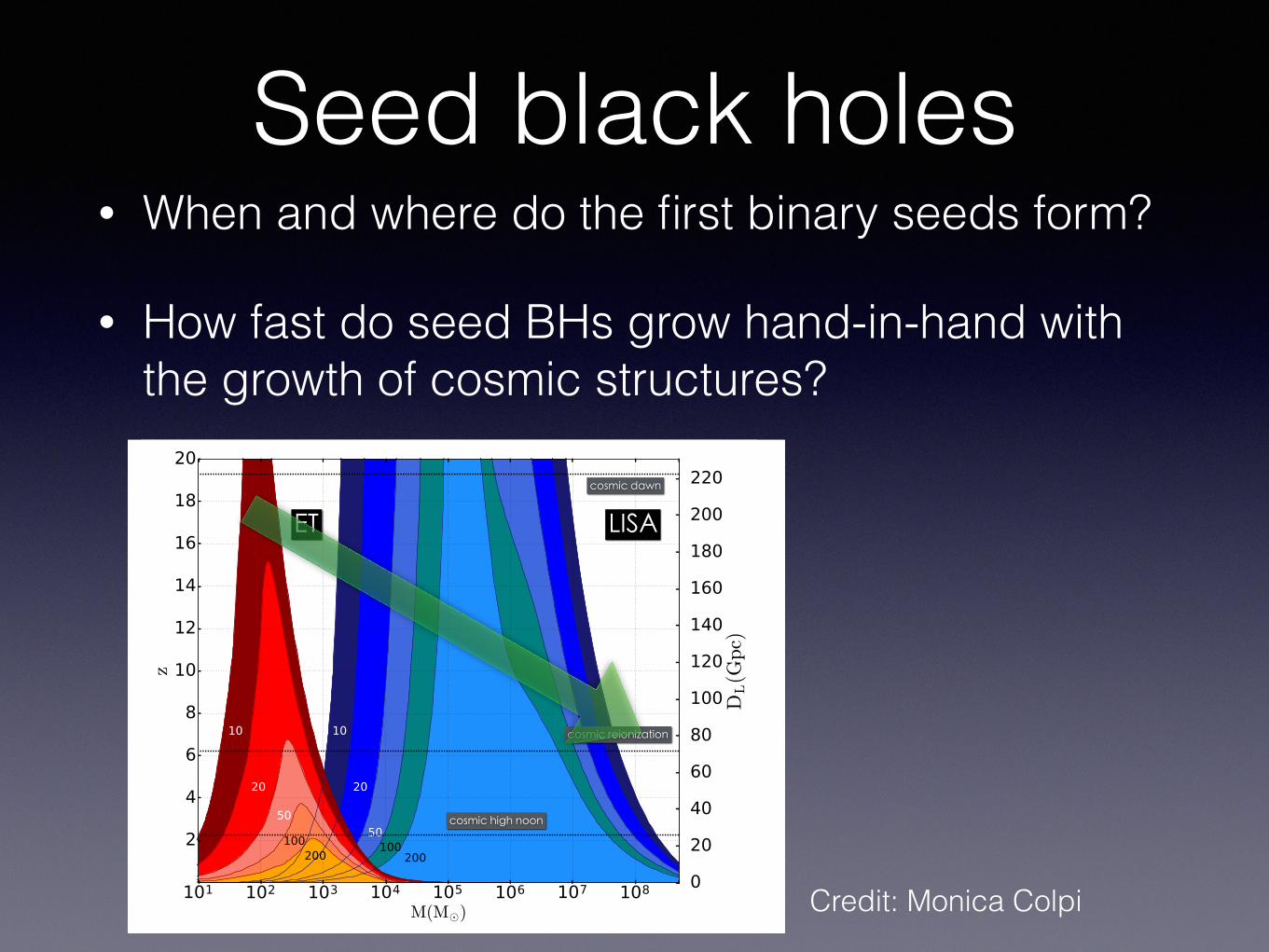
Seed black holes• When and where do the first binary seeds form?

• How fast do seed BHs grow hand-in-hand with the growth of cosmic structures?

10

Credit: Monica Colpi

Multi-messenger observations• What is the contribution of NS-NS and/or NS-BH

mergers to r-process elemental production? • How does this vary with redshift? • Where in the galaxies do these mergers occur

and what does the location tell us?

11

Kasen et al 2017

Neutron Stars• Neutron star structure from observation of

binaries, and continuous waves.

12

10 50 100 500 1000 500010-25

10-24

10-23

10-22

10-21

f HHzL

S nHfL

and2Hf»héHfL»L1ê2

BH-BHInitia

l LIGO

AdvancedLIGO

Einstein Telescope

What are we trying to put into waveform models? NSNS

3

10 50 100 500 1000 500010-25

10-24

10-23

10-22

10-21

f HHzL

S nHfL

and2Hf»héHfL»L1ê2

NS-NS EOS HBInitia

l LIGO

AdvancedLIGO

Einstein Telescope

effectively point-particle

tidal effects

AFTER NSNS merger

NS-NS merger

Credit: J Read

Neutron Stars• Neutron star structure from observation of

binaries, and continuous waves.

13

decomposition in the appendix. One can clearly recognise that in the early postmerger phasethere are two distinct frequencies simultaneously contributing to the GW signal. The fre-quency of the dominant remnant oscillation is present for many milliseconds. The secondarypeak at fspiral is generated within the first few milliseconds, when the antipodal bulges arepronounced (see figure 2). There is no evidence for a strong time variation of the frequencies,especially of the dominant frequency, which was suggested as an explanation for the structureof the GW spectrum in [52, 53]. A roughly constant dominant frequency has also been seenin [54].

The information in the time-frequency map of the GW signal can be related to thedynamical behaviour of the remnant, which we illustrate by the evolution of the rest-massdensity in the equatorial plane for the same simulation (see figure 2). The time step of thedifferent snapshots are marked in the time-frequency map (figure 1) by vertical lines. Evi-dently, the presence of antipodal bulges at the outer remnant coincides with the presence ofpower at fspiral in the time-frequency map. It is apparent that the fspiral feature is initiallyparticularly strong exceeding even the emission at fpeak; the antipodal bulges are strongestduring and immediately after merging and the spiral deformation forming the bulges initiallycomprises large parts of the remnant (see upper right panel in figure 2). In figure 2, theantipodal bulges complete approximately one orbit from the top right to the bottom left panelin about 1.2 ms. Thus, the orbital frequency = =f 1 1.2 ms 0.833 kHzbulges is expected toproduce a peak at = =f f2 1.67 kHzspiral bulges , where a peak is found in the spectrum (seefigure 1). For comparison we also show the time-frequency analysis for the SFHO EoS andcomponent masses 1.35–1.35 :M in figure 3. Here the secondary peak at 2.2 kHz likely arisesfrom the -f2 0 feature. An examination of the hydrodynamical data for this model reveals anfbulges of about 1.25 kHz (resulting in »f 2.5spiral kHz), whereas the frequency of the quasi-radial mode is =f 1.0 kHz0 , and thus the -f2 0 peak is expected to occur at about 2.2 kHz.

The above findings on the time-frequency characteristics of the fspiral peak are consistentwith the explanations of its origin presented in [42]. The fspiral feature is particularly strong for

Figure 1. Time-frequency analysis for the TM1 1.35+1.35 waveform for an optimallyoriented source at 50 Mpc. The top and right panels show the time-domain waveform-component +h and its Fourier magnitude spectrum, respectively. The time-frequencymap is constructed from the magnitudes of the coefficients of a continuous wavelettransform using a Morlet basis. Horizontal red lines emphasise the locations of the peakfrequency fpeak and the secondary peak which, in this case, corresponds to fspiral (seetext and figure 2). The vertical lines correspond to the time steps of the four panels infigure 2.

Class. Quantum Grav. 33 (2016) 085003 J A Clark et al

5

Clark et al 2016

Supernovae

• Can we distinguish the various phases of the supernova explosion?

• Can we determine the nuclear equation of state?

• Can we determine the progenitor mass?

14

Morozova et al 2018

Extreme GravityAlternative theories of gravity:

• New polarisations

• Graviton mass

• Lorentz violations

• Constraints on speed of standard and extra polarizations

15

Extreme GravityExotic compact objects

• Do exotic compact objects, such as boson stars and strange stars, exist?

• Can we observe multiple ringdown modes to verify BH no hair theorem?

• Do singularities and event horizons really form?

16

350Msunbinary@100Mpc

London et al 2014

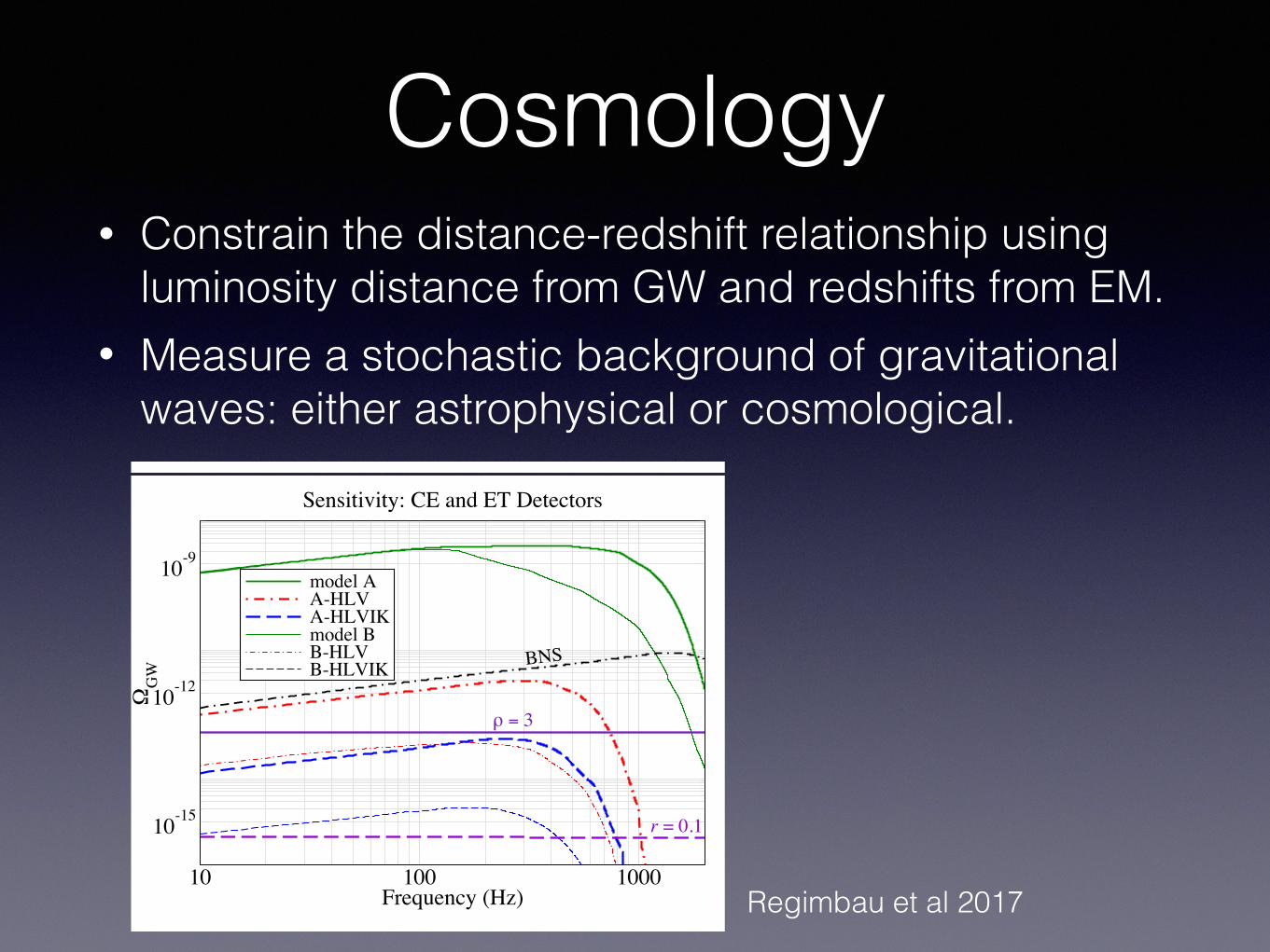
Cosmology• Constrain the distance-redshift relationship using

luminosity distance from GW and redshifts from EM. • Measure a stochastic background of gravitational

waves: either astrophysical or cosmological.

17

10 100 1000Frequency (Hz)

10-9

ΩG

W

model AA-HLVA-HLVIKmodel BB-HLVB-HLVIK

Sensitivity: Advanced Detectors

ρ = 3

BNS


10-9Ω

GW


Sensitivity: A+ Detectors

ρ = 3

BNS


10-15

10-12

10-9

ΩG

W


Sensitivity: CE and ET Detectors

r = 0.1

BNS

ρ = 3

FIG. 2. Energy density spectrum ⌦GW in GWs from unde-tected BBHs (⇢T < 12) with in Advanced (top plot), A+(middle plot) and third generation (bottom plot) detectors.Solid (green) curves are the total backgrounds for models A(thick lines) and B (thin lines), respectively, when detectedBBH signals are not removed from the data, so they are thesame in each plot. We see that in the tens of Hz regionone obtains the characteristic f2/3 slope. The cosmologicalbackground from inflation assuming a tensor-to-scalar ratio ofr = 0.1 is shown for comparison, and confusion backgroundfrom unresolved binary neutron stars, assuming an averagelocal rate of 60 Gpc�3 yr�1 [63]. The horizontal solid line isthe minimal flat spectrum that can be detected with ⇢ = 3with a 5-detector network after five years.

with third generation detectors opens up the possibilityto observe the PGWB.

Acknowledgments — We thank Thomas Dent, VukMandic and Alan Weinstein for comments. B.S.S ac-knowledges the support of Science and Technologies Fa-cilities Council grant ST/L000962/1. N.C received sup-port from NSF grant PHY-1505373. M.E., E.K. andS.V. acknowledge the support of the National ScienceFoundation and the LIGO Laboratory. LIGO was con-structed by the California Institute of Technology andMassachusetts Institute of Technology with funding fromthe National Science Foundation and operates under co-operative agreement PHY-0757058T.R acknowledges theLIGO Visitors Program and is grateful to X.O. for usefuldiscussions. This article has been assigned LIGO Docu-ment number P1600323.

[1] L. P. Grishchuk, Soviet Journal of Experimental and The-oretical Physics 40, 409 (1975).

[2] L. P. Grishchuk, Phys. Rev. D 48, 3513 (1993), gr-qc/9304018.

[3] A. A. Starobinskii, ZhETF Pisma Redaktsiiu 30, 719(1979).

[4] M. Gasperini and G. Veneziano, Astroparticle Physics 1,317 (1993), hep-th/9211021.

[5] A. Buonanno, M. Maggiore, and C. Ungarelli, Phys. Rev.D 55, 3330 (1997), gr-qc/9605072.

[6] J.-F. Dufaux, D. G. Figueroa, and J. Garcıa-Bellido,Phys. Rev. D 82, 083518 (2010), arXiv:1006.0217 [astro-ph.CO].

[7] T. Damour and A. Vilenkin, Phys. Rev. D 71, 063510(2005), hep-th/0410222.

[8] X. Siemens, V. Mandic, and J. Creighton, Physical Re-view Letters 98, 111101 (2007), astro-ph/0610920.

[9] S. Olmez, V. Mandic, and X. Siemens, Phys. Rev. D 81,104028 (2010), arXiv:1004.0890 [astro-ph.CO].

[10] T. Regimbau, S. Giampanis, X. Siemens, and V. Mandic,Phys. Rev. D 85, 066001 (2012), arXiv:1111.6638 [astro-ph.CO].

[11] C. Caprini, R. Durrer, and G. Servant, Phys. Rev. D 77,124015 (2008), arXiv:0711.2593.

[12] C. Caprini, R. Durrer, T. Konstandin, and G. Servant,Phys. Rev. D 79, 083519 (2009), arXiv:0901.1661 [astro-ph.CO].

[13] C. Caprini, R. Durrer, and G. Servant, Journal ofCosmology and Astroparticle Physics 12, 024 (2009),arXiv:0909.0622 [astro-ph.CO].

[14] T. Regimbau, Research in Astronomy and Astrophysics11, 369 (2011), arXiv:1101.2762 [astro-ph.CO].

[15] M. Punturo et al., Classical Quantum Gravity 27, 194002(2010).

[16] B. P. Abbott, R. Abbott, T. D. Abbott, M. R. Aber-nathy, K. Ackley, C. Adams, P. Addesso, R. X. Adhikari,V. B. Adya, C. A↵eldt, and et al., ArXiv e-prints (2016),arXiv:1607.08697 [astro-ph.IM].

[17] C. Cutler and J. Harms, Phys. Rev. D 73, 042001 (2006),gr-qc/0511092.

[18] J. Harms, C. Mahrdt, M. Otto, and M. Prieß, Phys. Rev.

5

Regimbau et al 2017

Modelling and analysis challenges

• Precision GW astronomy requires accurate waveform models

• Require accurate models with additional GW modes, precession, high mass ratio, eccentricity

• Inclusion of matter and neutrino effects

• Expanded length of waveforms, larger template banks, overlapping weak signals

18

Detectors and Networks

19

Class. Quantum Grav. 29 (2012) 124013 B Sathyaprakash et al

100

101

102

103

104

Frequency (Hz)

10-25

10-24

10-23

10-22

10-21

Stra

in (H

z-1/2

) ET-BET-D

100 101 102 103 1041

2

5

10

20

50

100

200

0.20

0.37

0.79

1.40

2.40

5.20

9.40

17.00

Total m ass in M

Lum

inos

ity

dist

ance

Gp

c

Redsh

iftz

Sky ave. dist . vs Phys. M, 0.25, 0.75

Sky ave. dist . vs Obs. M, 0.25, 0.75

Sky ave. dist . vs Phys. M, 0.25, 0

Sky ave. dist . vs Obs. M, 0.25, 0

Figure 4. (Left) ET’s strain sensitivity for two optical configurations: ET-B [24] and ET-D [25].(Right) ET-B’s distance reach for compact binary mergers as a function of the observed total mass(blue dashed curves) and intrinsic total mass (red solid curves) for non-spinning binaries (lowercurves) and binaries with dimensionless spins of 0.75 (upper curves).

Since the detector tensors are given by

di j1 = 1

2

(ei

2e j3 − ei

3e j2

), di j

2 = 12

(ei

3e j1 − ei

1e j3

), di j

3 = 12

(ei

1e j2 − ei

2e j1

),

where e1, e2 and e3 are the unit vectors along the arms of the detectors as in figure 2. It is easyto see that

∑A hA = 0, irrespective of the direction in which the radiation is incident or its

polarization. Thus, the sum of the detector outputs∑

A xA(t) =∑

A[nA(t)+hA(t)] =∑

A nA(t)contains only the sum of the three noise backgrounds. This is the null data stream, which iscompletely devoid of any GWs. It is like the dark-current of an optical telescope. It can beused to veto spurious events [22], to estimate the noise spectral density of the detectors (whichis critical for a signal-dominated instrument such as the ET) and to detect a stochastic GWbackground that may be buried in the data streams [21].

The ET has also the ability to resolve the wave’s two polarization states. It isstraightforward to invert ET’s response functions hA = FA

+ h+ + FA× h×, A = 1, 2, 3, to

solve for the signal’s two polarizations. We would not have direct access to hA but only todetector outputs xA = hA + nA whose linear combinations could be used to get estimates ofthe two polarizations.

For a pair of misaligned L-shaped detectors (i.e. detectors that are not rotated relative toeach other by multiples of π/2 rad), there is no linear combination of their responses that givesa null data stream. Nevertheless, as noted before, two interferometers sharing common arms(as in the LIGO Hanford setup) can be used to construct a sky-independent null stream. Evenso, a triangular topology can provide the same information and yet incur lower infrastructurecosts. If one is going to build two pairs of L-shaped detectors, then it makes sense to buildthem at geographically widely separated sites, as that would help in obtaining at least partialinformation about source position, which would obviously increase the science reach over asingle-site ET.

3.3. ET’s sensitivity

Figure 4(left) shows the sensitivity of each V-shaped detector in the ET, for two differentoptical configurations. The red solid curve, labeled ET-D, shows the sensitivity of a xylophoneconfiguration [23] in which two interferometers are installed in each V of the triangle: one thathas good high-frequency sensitivity and the other with good low-frequency sensitivity. Theblue dashed curve, labeled ET-B, shows the best possible sensitivity for a single detector in each

9

Impacts for binary mergers

Merger physicsLocalisation

Mass accuracyHigh mass/high z

Number of sources

Detectors and Networks• Networks obviously important for source localization

• Also impact ability to measure distance/redshift (and hence mass) and binary orientation

20

GW150914 with future detectors 9

Figure 4. The magnification of the region surrounding the true position. Whilefigure 3 shows the large scale localisation, this plot illustrates the di↵erences between3, 4, and 5-detector set-ups, which continuously shrink the area while remaining centredon the true location. Noteworthy is also that even at low sensitivity AdVirgo is ableto shrink the area massively and collapse the annulus into a region with the diametercomparable to the width of the 2-detector ring. The increased sensitivity has a greaterimpact in the 3-detector set-up as the improvements in AdVirgo are much larger.

Figure 5. The posterior distributions of the luminosity distance to the source and theinclination angle, for one simulated signal. The distance measurement covers a widerange of values, as the distance prior is uniform in volume and the distance is not verywell measured and degenerate with other extrinsic parameters. The inclination angle isonly weakly constrained at current sensitivities or with only two detectors. While thedegeneracy between face-on and -o↵ orientations can be broken with a third detectorat higher sensitivities, the width of the peak decreases only from ⇡ ⇡/4 to ⇡ ⇡/7.Qualitative di↵erences with the posterior peaking close to the maximum appear onlyonly once a fourth detector in an advantageous location is added.

Gaebel & Veitch 2017

Summary• First GW observations have provided spectacular

scientific payoffs • 3G/ET observations will provide a new window, e.g.

• merger history of universe • BBH spectroscopy • Neutron star structure • Supernovae • Nucleosynthesis

• Work ongoing to produce 3G science case

21

et and 3g science

Documents